Ryan Shiroma MATH 285 Homework 2

1: Multidimensional Scaling

(a) Below is the code for the MDS function. It takes the distance matrix X and k dimensions ofthe output space, and returns the mapped coordinates Y and its associated Kruskal’s stress.

MDS Function1 function [Y,stress] = mds(X,k)2 points=size(X,1); %number of points3 means=repmat(mean(X),points,1); %4 l_i_dot=means; % column means5 l_dot_j=means'; % row means6 l_dot_dot=ones(points)*mean(mean(X)); % matrix mean7 l_i_j=X;8 L=(l_i_dot.^2+l_dot_j.^2−l_dot_dot.^2−l_i_j.^2)/2; %compute the L matrix9 [U,D]=eig(L); % get the eigen−values and eigen vectors

1011 reverse=points:−1:1; % sort in descending order (eig() returns ascending order

)12 U=U(:,reverse);13 D=diag(nonzeros(D(:,reverse)));1415 Y=U*sqrt(D); % compute the Y matrix16 Y=Y(:,1:k); % pull points in only the first k dimensions1718 % KRUSCAL STRESS19 numerator=0;20 denominator=0;2122 for i=1:points % loop through all rows23 % Loop through columns from i+1 to the end24 % To make this loop twice as fast, we only need to calculate the25 % scores between points we haven't calculated yet.26 for j=i+1:points27 numerator=numerator+(X(i,j)−sqrt(sum((Y(i,:)−Y(j,:)).^2)))^2;28 denominator=denominator+X(i,j)^2;29 end30 end31 stress=sqrt(numerator/denominator); % calculate the final stress number32 return;

1

Ryan Shiroma MATH 285 Homework 2

Using our MDS function we can now do mutli-dimensional scaling on the Chinese city distancedata. The steps in the script are:1) Load data2) Run MDS3) Rotate the points so that they match the actual map4) Plot the points

MDS Script1 load ChineseCityData.mat;2 [Y,stress]=mds(dists,2); % run the MDS function3 % We now rotate the mapping so that it looks close to a real map of China4 % Chongqing and Urumqi seem to be at a 45 degree angle in relation to the5 % x axis on the map of China, so let's rotate the map to match this.67 a=Y(4,:)−Y(6,:);8 b=[1000,−1000];9 rads= −acos(a*b.'/norm(a)/norm(b)) ;

10 rot_matrix=[cos(rads), −sin(rads);sin(rads), cos(rads)];11 Y=Y*rot_matrix;1213 % plot the rotated Y points14 figure;15 img = imread('chinamap.jpg');16 image([−4600 2300],[2000 −2500],img);17 hold on;18 scatter(Y(:,1),Y(:,2));19 axis equal;20 grid on;21 text(Y(:,1), Y(:,2), Cities,'VerticalAlignment','bottom','HorizontalAlignment'

,'right');22 title('2D mapping from a distance matrix');23 xlabel('km''s from the center'); ylabel('km''s from the center');

1 >> stress23 stress =45 0.0807

The Kruskal stress score was 0.0807 which as a rule of thumb places this in the “good” range.

2

Ryan Shiroma MATH 285 Homework 2

−2500 −2000 −1500 −1000 −500 0 500 1000 1500

−2000

−1500

−1000

−500

0

500

1000

Beijing

Tianjin

Shanghai

Chongqing

Hohhot

Urumqi

Lhasa

Yinchuan

Nanning

Harbin

Changchun

Shenyang

2D mapping from a distance matrix

km’s from the center

km’s

from

the

cent

er

The MDS map follows the map of China I found online fairly closely. In theory, these two mapsmight’ve lined up exactly since both the MDS map and this image need to project points in R3

into R2. The Chinese map image may be distorted slightly due to the many ways to represent amap, causing the points not to match up.

Beijing

Tianjin

Shanghai

Chongqing

Hohhot

Urumqi

Lhasa

Yinchuan

Nanning

Harbin

Changchun

Shenyang

2D mapping from a distance matrix

km’s from the center

km’s

from

the

cent

er

−4000 −3000 −2000 −1000 0 1000 2000

−2500

−2000

−1500

−1000

−500

0

500

1000

1500

2000

(b) Unfortunately we wouldn’t be able to construct a world map based on locations around theworld. We can “flatten” a smaller portion of the world (like a single country) into a 2D map whilepreserving pairwise distance fairly well, but not as well if the points are formed around a sphere.The Kruskal score to a world airport mapping would probably be very bad.

3

Ryan Shiroma MATH 285 Homework 2

2: ISOmap

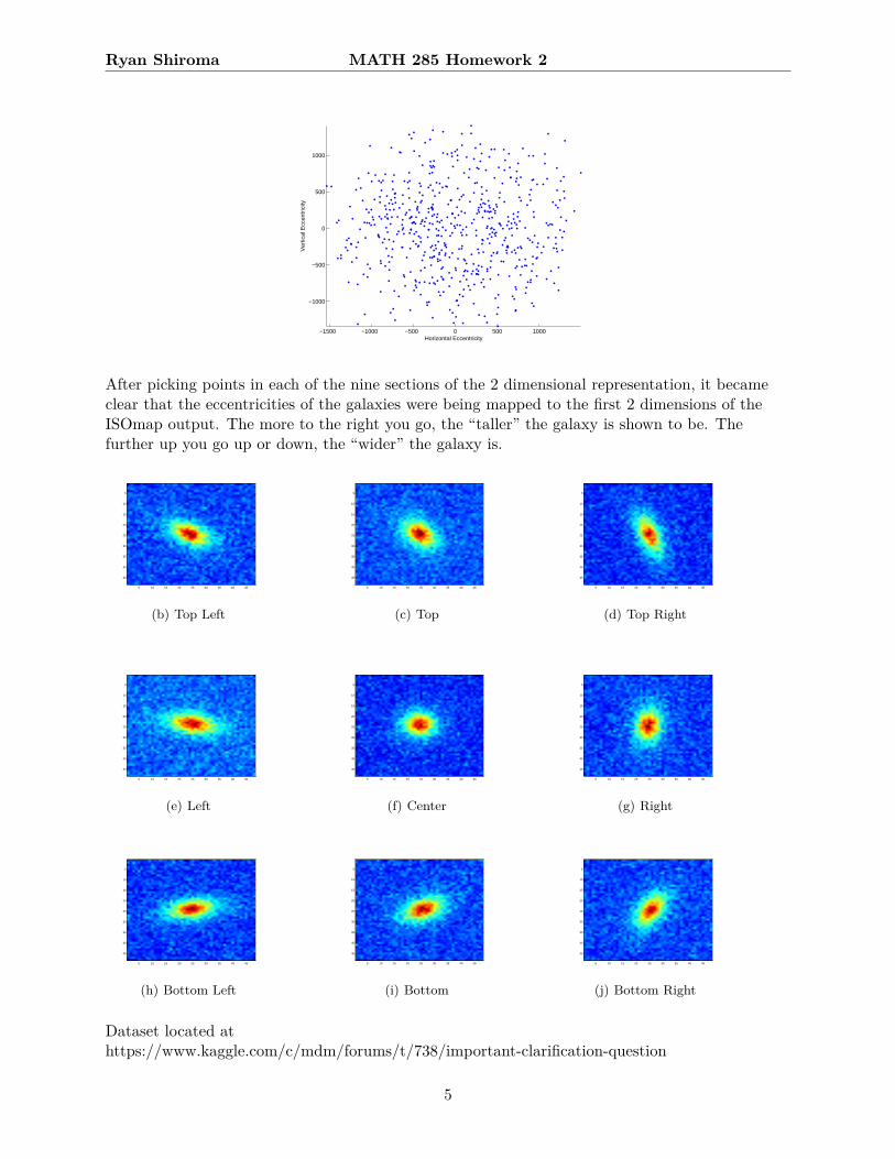
(a) Galaxies Dataset The dataset I used was found on kaggle.com. The original goal of thiskaggle.com competition was to measure the ellipticity of the galaxies in the test set. Theellipticity of a galaxy is a measure of the longest and shortest diameters of the elliptical shape of agalaxy. The dataset consists of 40,000 48x48 grayscale images of galaxies. I only use the first 600for this analysis.I reduced the dimension on this dataset with standard PCA but received a similar output to theMNIST ones scatterplot from the first homework assignment. It seems that using MDS orISOmap would result in a better interpretation.

−3500 −3000 −2500 −2000 −1500 −1000 −500 0 500−250

−200

−150

−100

−50

0

50

100

150

200

250data plotted against the first two principal components

(a) Regular-PCA Scatterplot

ISOmap Script1 % First create an image matrix from the png files. Each png file is a 48x482 % grayscale image. I am using the first 600 images from the dataset.3 file = dir('galaxy');4 images=zeros(2304,600);5 for k = 3 : 6036 images(:,k−2) = reshape(imread(fullfile('galaxy', file(k).name)),2304,1);7 end89 % calculate the distance matrix

10 D = L2_distance(images, images, 1);1112 % Run the ISOmap code13 options = struct();14 options.dims = 1:5;15 options.display = 0;16 options.overlay = 0;17 Y_isomap = Isomap(D, 'k', 7, options);1819 % Plot the ISOmap output on the first 2 dimensions20 figure; gcplot(Y_isomap.coords{2}');21 xlabel('Horizontal Eccentricity');ylabel('Vertical Eccentricity');

4

Ryan Shiroma MATH 285 Homework 2

−1500 −1000 −500 0 500 1000

−1000

−500

0

500

1000

Horizontal Eccentricity

Ver

tical

Ecc

entr

icity

After picking points in each of the nine sections of the 2 dimensional representation, it becameclear that the eccentricities of the galaxies were being mapped to the first 2 dimensions of theISOmap output. The more to the right you go, the “taller” the galaxy is shown to be. Thefurther up you go up or down, the “wider” the galaxy is.

5 10 15 20 25 30 35 40 45

5

10

15

20

25

30

35

40

45

(b) Top Left

5 10 15 20 25 30 35 40 45

5

10

15

20

25

30

35

40

45

(c) Top

5 10 15 20 25 30 35 40 45

5

10

15

20

25

30

35

40

45

(d) Top Right

5 10 15 20 25 30 35 40 45

5

10

15

20

25

30

35

40

45

(e) Left

5 10 15 20 25 30 35 40 45

5

10

15

20

25

30

35

40

45

(f) Center

5 10 15 20 25 30 35 40 45

5

10

15

20

25

30

35

40

45

(g) Right

5 10 15 20 25 30 35 40 45

5

10

15

20

25

30

35

40

45

(h) Bottom Left

5 10 15 20 25 30 35 40 45

5

10

15

20

25

30

35

40

45

(i) Bottom

5 10 15 20 25 30 35 40 45

5

10

15

20

25

30

35

40

45

(j) Bottom Right

Dataset located athttps://www.kaggle.com/c/mdm/forums/t/738/important-clarification-question

5

Ryan Shiroma MATH 285 Homework 2

3: Dijkstra’s Algorithm

Step 1 Start at Node O.Create paths to nodes A, B, and C and assign the distances to each node.

Step 2 Since A has the shortest distance, we move to Node A.Let’s first create paths to node F, D, and B. The distance to B from A is now 4 which is lessthan the current distance of 5. We can then replace the distance to B with 4 and removethe path from O to B.

Step 3 Nodes B and C have the next shortest distances. We’ll arbitrarily choose Node B.Let’s create paths from node B to nodes C, E, and D. The path to node C through B is thesame as the current distance to C, therefore we can remove this path. The path to Dthrough node B is 8, which is shorter than the current path from A. We can remove the edgefrom A to D as well. Finally, the path to E doesn’t exist yet so we give it the distance of 7.

6

Ryan Shiroma MATH 285 Homework 2

Step 4 The next shortest path is from Node C. The edge from node C to node B is not neededsince we have already seen node B. The distance to node E from node C is 4+4=8 which islarger than the current distance of 7 so we can disregard that path as well.

Step 5 Node E has the next shortest path. The distance to node D through node E is larger thanthe current distance of 8 so we can ignore that edge. The path to node T doesnt exist yet sowe can creat that path with a distance of 7+7=14.

Step 6 Node D has the next shortest distance with a distance of 8. The only node connected tonode D that hasn’t be seen yet is node T. Going through node D, the distance to node T isonly 13, which is less than the current distance of 14 so we can remove the edge from nodeE to node T.

7

Ryan Shiroma MATH 285 Homework 2

Step 7 Of the two remaining nodes, T and F, Node T has the shorter distance. The only edgeremaining is the edge from node T to node F. The distance to node F doesnt decrease whengoing through node T so we can ignore this final edge.

Done We have now seen all nodes and can now see the shortest paths from node O to any othernode.

Node O to:A: distance = 2. path: O to AB: distance = 4. path: O to A to BC: distance = 4. path: O to CD: distance = 8. path O to A to B to DE: distance = 7. path: O to A to B to EF: distance = 14. path: O to A to FT: distance = 13. path: O to A to B to D to T

8

Ryan Shiroma MATH 285 Homework 2

4: Kernel PCA

(a) The kPCA function takes the input data (centered or uncentered) and the reduced dimensionk, and returns the Y matrix of points in the dimension k.

Kernel PCA Function1 function Y = kPCA(X,k)2 n=size(X,1);3 X_tilde=X−repmat(mean(X,1),n,1); % compute a centered X matrix45 % This section is used to compute an initial value for the6 % parameter, sigma7 dist=zeros(n,n); % initialize the distance matrix8 for i=1:n9 for j=i+1:n

10 dist(i,j)=sqrt(sum((X_tilde(i,:)−X_tilde(j,:)).^2));11 end12 end13 dist=dist + dist';14 mean_sim=mean(sort(dist,1),2); %for each point, sort columns by distance15 % Taking Dr. Chen's suggestion, we'll take the average of the 8th nearest16 % neighbor. We use nine here since we don't count the point itself as17 % a "nearest neighbor"18 sigma =mean_sim(9);1920 % We now can compute the K matrix. We use our own function "RBF" to clean21 % up the code a little bit.22 K=zeros(n,n);23 for i=1:n24 % Since K is symmetric, we only need to compute an upper triangular25 % matrix and just add the transpose.26 for j=i:n27 K(i,j)= RBF(X_tilde(i,:),X_tilde(j,:),sigma);28 end29 end30 K=K + K'−diag(diag(K));% compute K from the upper triangular K matrix.3132 one=ones(n,n); % compute the K tilde matrix33 K_tilde=K−(1/n)*K*one −(1/n)*one*K +(1/n)^2*one*K*one;3435 % find the eigenvalues/vectors that satisfy K*V_i = n*lambda*V_i.36 % We also need to resort the eigenvectors by largest eigenvalues.37 [V,D]=eig(K_tilde/n);38 [~,index]=sort(diag(D),'descend');39 V=V(:,index);4041 % finally compute the Y matrix42 Y=K*V(:,1:k);43 return;

9

Ryan Shiroma MATH 285 Homework 2

RBF Function1 function mapping = RBF(xi,xj,sigma)2 mapping=exp( −sqrt(sum((xi−xj).^2))/(2*sigma^2));3 return;

Kernel PCA Script1 load kernelpca_data2 % Plot the original data3 figure;plot(X(labels==1,1),X(labels==1,2),'.b','MarkerSize',10);4 hold on;5 plot(X(labels==2,1),X(labels==2,2),'.g','MarkerSize',10);6 title 'Kernel PCA Data';7 legend('Inside Cluster','Outside Cluster')89 Y=kPCA(X,2); % Run the kernel PCA function with dimension 2

1011 % Plot the newly mapped data on the first two dimensions12 figure;plot(Y(labels==1,1),Y(labels==1,2),'.b','MarkerSize',10);13 hold on;14 plot(Y(labels==2,1),Y(labels==2,2),'.g','MarkerSize',10);15 title 'Kernel PCA Data(Remapped)';16 legend('Inside Cluster','Outside Cluster')

−3 −2 −1 0 1 2 3 4−3

−2

−1

0

1

2

3

4Kernel PCA Data

Inside ClusterOutside Cluster

(k) Original Data

−0.5 0 0.5 1 1.5 2 2.5 3 3.5−1.5

−1

−0.5

0

0.5

1

1.5Kernel PCA Data(Remapped)

Inside ClusterOutside Cluster

(l) Remapped Data

Figure 1: Kernel PCA

The data can now clearly be separated with lines. This can now be easily clustered without anyissues. We can test whether this is true by running the kmeans script on the next page.

10

Ryan Shiroma MATH 285 Homework 2

k-means clustering on top of Kernel PCA1 k=22 [labels_kmeans,C,scatter] = kmeans(X,k,'Replicates',10);3 error=computing_percentage_of_misclassified_points(labels,labels_kmeans)4 figure; gcplot(X, labels_kmeans); axis equal56 [labels_kmeans,C,scatter] = kmeans(Y,k,'Replicates',10);7 error=computing_percentage_of_misclassified_points(labels,labels_kmeans)8 figure; gcplot(Y, labels_kmeans); axis equal

Running the k-means code on these data points shows that if we were to cluster the original dataset, we could potentially get an error of 34%. But running k-means on the remapped data set, wesee an error rate of 0%.

−3 −2 −1 0 1 2 3 4

−2

−1

0

1

2

3

(a) Original Data (error = 34.13%)

0 0.5 1 1.5 2 2.5 3

−1

−0.5

0

0.5

1

(b) Remapped Data (error = 0%)

Figure 2: k-means over Kernel PCA

11

Ryan Shiroma MATH 285 Homework 2

5: k-means

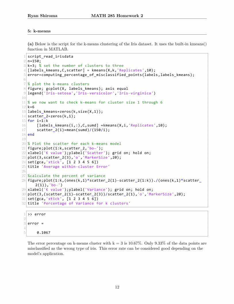
(a) Below is the script for the k-means clustering of the Iris dataset. It uses the built-in kmeans()function in MATLAB.

1 script_read_irisdata2 n=150;3 k=3; % set the number of clusters to three4 [labels_kmeans,C,scatter] = kmeans(X,k,'Replicates',10);5 error=computing_percentage_of_misclassified_points(labels,labels_kmeans);67 % plot the k−means clusters8 figure; gcplot(X, labels_kmeans); axis equal9 legend('Iris−setosa','Iris−versicolor','Iris−virginica')

1011 % we now want to check k−means for cluster size 1 through 612 k=613 labels_kmeans=zeros(k,size(X,1));14 scatter_2=zeros(k,1);15 for i=1:k16 [labels_kmeans(i,:),C,sumd] =kmeans(X,i,'Replicates',10);17 scatter_2(i)=mean(sumd)/(150/i);18 end1920 % Plot the scatter for each k−means model21 figure;plot(1:k,scatter_2,'bo−');22 xlabel('K value');ylabel('Scatter'); grid on; hold on;23 plot(3,scatter_2(3),'o','MarkerSize',20);24 set(gca,'xtick', [1 2 3 4 5 6])25 title 'Average within−cluster Error'2627 %calculate the percent of variance28 figure;plot(1:k,(ones(k,1)*scatter_2(1)−scatter_2(1:k))./(ones(k,1)*scatter_

2(1)),'bo−')29 xlabel('K value');ylabel('Variance'); grid on; hold on;30 plot(3,(scatter_2(1)−scatter_2(3))/scatter_2(1),'o','MarkerSize',20);31 set(gca,'xtick', [1 2 3 4 5 6])32 title 'Percentage of Variance for k clusters'

1 >> error23 error =45 0.1067

The error percentage on k-means cluster with k = 3 is 10.67%. Only 9.33% of the data points aremisclassified as the wrong type of iris. This error rate can be considered good depending on themodel’s application.

12

Ryan Shiroma MATH 285 Homework 2

−3 −2 −1 0 1 2 3−1.5

−1

−0.5

0

0.5

1

1.5

Iris−setosaIris−versicolorIris−virginica

(a) Actual clusters (Iris types)

−3 −2 −1 0 1 2 3−1.5

−1

−0.5

0

0.5

1

1.5

(b) k-means clusters with k = 3 (error = 10.67%)

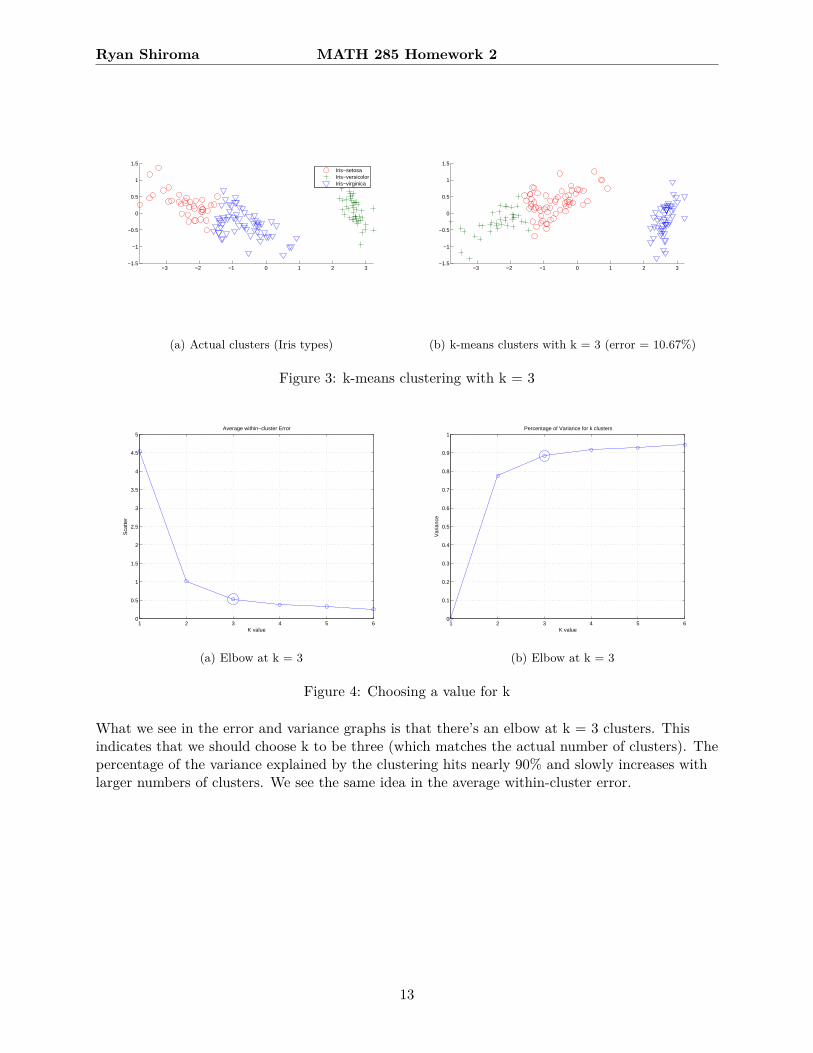
Figure 3: k-means clustering with k = 3

1 2 3 4 5 60

0.5

1

1.5

2

2.5

3

3.5

4

4.5

5

K value

Sca

tter

Average within−cluster Error

(a) Elbow at k = 3

1 2 3 4 5 60

0.1

0.2

0.3

0.4

0.5

0.6

0.7

0.8

0.9

1

K value

Var

ianc

ePercentage of Variance for k clusters

(b) Elbow at k = 3

Figure 4: Choosing a value for k

What we see in the error and variance graphs is that there’s an elbow at k = 3 clusters. Thisindicates that we should choose k to be three (which matches the actual number of clusters). Thepercentage of the variance explained by the clustering hits nearly 90% and slowly increases withlarger numbers of clusters. We see the same idea in the average within-cluster error.

13