Embed Size (px)
Citation preview

A review of hydrologic models for flash floodwarning system in southwest Saudi Arabia.
Item Type Thesis-Reproduction (electronic); text
Authors Al-Haratani, Eisa Ramadan, 1958-
Publisher The University of Arizona.
Rights Copyright © is held by the author. Digital access to this materialis made possible by the University Libraries, University of Arizona.Further transmission, reproduction or presentation (such aspublic display or performance) of protected items is prohibitedexcept with permission of the author.
Download date 20/05/2018 22:20:15
Link to Item http://hdl.handle.net/10150/191312

A REVIEW OF HYDROLOGIC MODELS FOR FLASH FLOODWARNING SYSTEM IN SOUTHWEST SAUDI ARABIA
by
Eisa R. Al-Haratani
A Professional Paper Submitted to the Faculty of the
SCHOOL OF RENEWABLE NATURAL RESOURCES
in Partial Fulfillment of the Requirements
For the Degree of
MASTER OF SCIENCE
WITH A MAJOR IN WATERSHED MANAGEMENT
in the Graduate College
THE UNIVERSITY OF ARIZONA
1988

This professional paper has been approved or the dateshown
/)(///7..).4i
Date
Pe r FfolliottProfessor of Watershed Management
STATEMENT BY AUTHOR
This professional paper has been submitted inpartial fulfillment of requirements for an advanceddegree at The University of Arizona and is deposited inthe University Library to be made available toborrowers under rules of the Library.
Brief quotations from this paper are allowablewithout special permission, provided that accurateacknowledgement of source is made. Requests forpermission for extended quotation from or reproductionof the manuscript in whole or in part may be granted bythe head of the major department or the Dean of theGraduate College when in his or her judgment theproposed use of the material is in the interests ofscholarship. In all other instances, however,permission must be obtained from the author.
ThSigned:
APPROVAL BY GRADUATE COMMITTEE
illip Guertin ateAsst. Prof. in Watershed Management

DEDICATION
Dedicated to my father Ramadan, mother, Naima, my
wife Hanan, and my children, Ramadan and Reham. To them
I reserve my deepest gratitude. This paper must seem a
modest Consolation for all the inconvenience and
hardships they all have gone through to make this
possible.

ACKNOWLEDGEMENTS
It gives me great pleasure to acknowledge those
who have assisted me in carrying out this work,
especially the constructive criticisms regarding the
content and organization of this paper.
First and foremost, I would like to express my
sincerest gratitude to my major professor, Dr. Martin
Fogel, Who was ever available in my time of academic
and intellectual needs, who persevered to guide me with
this modest accomplishment. My association with him
has been a most stimulating experience in life and has
made my stay here with the University of Arizona an
enjoyable one.
I would like to thank Dr. Peter Ffolliott for his
academic support, likewise to Dr. Phil Guertin for his
assistance.
Special thanks goes to Dr. Walid Abed Rabboh for
his assistance and advise.
am also thankful to all my colleagues with the
School of Renewable Natural Resources, who helped me in
the preparation of this professional paper; Khalid M.
Arkanji, Raja Zarif, Mary Ann Pollisco-Botengan and
Ahmed Bakhashwain.
iv

Finally, I would like to express my appreciation
for the government of Saudi Arabia, particularly the
Meteorological and Environmental Protection
Administration, especially Dr. Abdulbar A. Al-Gain and
Dr. Nizar Tawfiq for their support.

TABLE OF CONTENTS
LIST OF FIGURES
LIST OF TABLES
ABSTRACT
INTRODUCTION
vii
viii
ix
1
The Asir Highlands 2
The Runoff Process 10
WATERSHED MODELS: A BACKGROUND 14
Soil Conservation Service Model 20
SCS TR-20 Watershed Model 30
Stanford Watershed Model 34
USDAHL-74 Model 37
ANSWERS Model 40
HEC-1 Model 44
THE AL-BAHA EXPERIMENTAL WATERSHEDS 46
Description of the Experimental Sites • • • 46
Experimental Data 50
DISCUSSION AND CONCLUSIONS 53
Conclusions 56
REFERENCES 58
vi

LIST OP FIGURES
1. A Map of Southwestern Saudi Arabia 4
2. Isohyetal Map of the Study Area 5
3. Relationship Between Rainfall and Runoff . . . 25
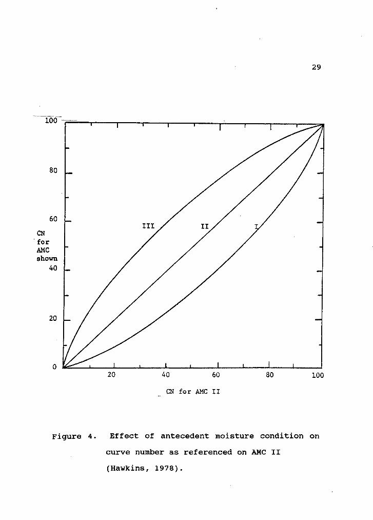
4. Effect of Antecedent Moisture Condition
on Curve Number as Referenced on AMC II . . . . 29
5. General Structure of SCS TR-20 Watershed Model 31
6. General Form of Stanford Watershed Model IV,
Showing Principal Storages and Flows 35
7. General Structure of USDAHL-74 Watershed Model 39
8. A Map of the Two Study Sites:
USGS and HEMA 48
vii

LIST OF TABLES
1. Antecedent Moisture Class Limits 28
2. Observed Versus Calculated Rainfall-Runoff
Data From Two Watersheds 51
viii

ABSTRACT
Various models have been applied in the analysis
of hydrologic conditions in different watershed areas.
The whole spectrum of models available as tools for
natural resource managers is because the use of
modeling techniques are limited for specific areas
and/or purposes. Constraints and limitations have to
be realized in order to properly select a model that
answers the needs of a certain locality, for a stated
goal.
It is the purpose of this paper to review existing
hydrologic models, and in the process, select the most
promising for application in the southwestern part of
Saudi Arabia for the purpose of designing flood control
and warning systems. The six models under
investigation are the SCS Method, SCS TR-20, Stanford,
USDA HL-74, HEC-1 and ANSWERS.
Based on the scope and limitations of each model,
as well as certain restrictions found within the area
of study, it became evident that the SCS models are the
most appropriate. This became more apparent having
considered the type of data input the models require
that can be provided for in the study area, as well as
the simplicity of the models and scale of application.
ix

1
INTRODUCTION
Different modeling techniques have been developed
and applied to estimate runoff from rainfall. Each
model was developed to fit and serve certain cases and
locations. Due to the lack of resources, poor research
activities and infrastructures in developing countries,
little work has been done in this field. Whenever
models are needed to be used in these countries, models
are imported from developed countries. The only
criterion often considered in selecting a model is the
researcher's familiarity with such a model.
The appropriateness and suitability of six models
will be evaluated, and their applicability for the
southwestern region of Saudi Arabia will be examined
and analyzed. In so doing, a description of each of
the six models and the study areas will be included in
the study. Different criteria will be applied in
evaluating the six models, namely required model
inputs, simplicity and the scale of model application.
Finally, a model or models will be selected and
recommended for adoption in southwestern Saudi Arabia
for purposes of designing flash flood warning systems
and flood control structures.

2
The Asir Highlands
Government records reveal that the total area of
Saudi Arabia is about 2.2 million square miles.
Approximately 80 percent of the Arabian Penninsula
falls under Saudi Arabia.
The population of the Kingdom is distributed along
the eastern and western coasts especially in towns and
interior oases. The total population of the country is
around eight million, of which about 70 percent reside
in cities and towns.
The climate of Saudi Arabia is generally hot with
winds blowing from the east towards the Arabian Gulf.
Humidity is low, with the exception of the coastal
zones, where it reaches over 90 percent. During the
summer months, the average annual temperature is 35°C,
while in winter it is 25°C. There is a wide range in
maximum and minimum temperatures. Rainfall is scarce
in the northern two-thirds of Saudi Arabia. It is
unpredictable with great annual variations. Long
periods of drought are common. However, where there is
rainfall, it is stormy with occasional flash floods in
low land areas, especially in the southwestern part.
This part of Saudi Arabia experiences seasonal rainfall
that can be as high as 600 millimeters.

3
This study will focus on the southwestern part of
Saudi Arabia (Fig. 1), which has two distinct areas;
the western and eastern slopes, separated by the
escarpment ridge of the Asir mountains. The western
zone encompasses a coastal strip between the Red Sea
and the mountain range. The topography of the upstream
sections of the western slope wadis (valleys), are very
steep particularly near the escarpment. Consequently,
runoff is carried by incised wadis of limited capacity.
The surface material on the mountains is generally
impermeable, thus groundwater resources at the upstream
sections are negligible. As the drainage system enters
the foothills, the topography flattens, and the
alluvial wadi (valley) beds widen. The shallow
alluvial deposits begin to hold significant amounts of
groundwater. Figure 2 shows the isohyetal map of
annual precipitation for the area. The map indicates
the geographic variability over the western and eastern
slopes of the zone, as well as the location of
different wadis. This rainfall is stormy in nature and
bring flash floods to the area. Insofar as hydrologic
data are concerned, a few surface runoff stations are
located at the foothills side of the wadis. Most of
the runoff records vary from 1967 to the present, as
reported in Ministry of Agriculture and Water (1963-85)

4
BanOAftWir+
+J. Wavle
by +Al Ândah Ansg
Figure 1. A map of Southwestern Saudi Arabia.

AL LITH
KINGDOM OF SAU
RIS HAN
ESCARPMENTMETERS
2000-Re ANNUAL RUNOFF VOLUME
RN=NATURAL SURFACE RUNOFF
RG a ANNUAL GW RECHARGE
i-COASTALPLAIN
100Cs•
UPtANDS
LOCATION MAP OF THE STUDY AREA
Topography of the Southwest Zone
FIGURE (la) TOPOGRAPHIC SECTION OF THE— ZONE.
ESCARPMENT RIDGE
z
AL QUNPUDHAN
LEGEND:-
AL BIRK
•—•-n INTERNATIONAL BOUNDARY.
• WATERSHED REGION BOUNDARY.ISOHYET.
Al.
WESTERN DRAINAGE SYSTEM
JIZAN
5
Figure 2. Isohyetal map of the study area.

publications, with the exception of few stations which
have been in operation since 1953. In some wadis, it
is not possible to provide an accurate estimate of the
natural surface runoff because some amounts are
diverted for agricultural purposes. Furthermore, the
wadi runoff is measured in only one of the branches
(Sorman and Abdul Razzak, 1987).
Saudi Arabia is characterized to be arid and semi-
arid, generally having low and sporadic rainfall of
short duration and high intensity. The sharp reliefs
of the terrain induces extreme flood magnitudes.
The southwest region has a total area of about
250,000 square kilometers, of which 77 percent are
agricultural and 23 percent for nomadic stock raising.
The total population of the area is 502,000 and 84
percent are engaged in agricultural production with the
remaining 16 percent involved with handicrafts and
other commercial ventures.
The southeastern region of Saudi Arabia is within
a transitional meteorological zone that is invaded by
various air masses at different times of the year. In
winter, the area is observed to be under the influence
of westerly air masses from the Mediterranean Sea, and
is associated with depressions that settle over the
northern part of Saudi Arabia. During spring time, an

7
intertropical front moves northward, hence the area
comes under the influence of relatively moist southerly
airstreams that give rise to precipitation over the
escarpment. Southwestern Saudi Arabia, specifically
the study areas of HEMA and USGS watersheds, can be
classified into three climatic zones:
1. The mountains in terms of elevation are above
1500 meters having a mean annual temperature
of 16 to 21°C, with a relative humidity of
about 65 percent. Average annual rainfall is
about 300 to 400 millimeters. Above 2300
meters elevation, it had been noted that ice
and frost are present and the mean temperature
can go as low as below 0°C.2. The foothills region with elevation between
1000 to 1500 meters, has a mean annual
temperature of about 25°C. Average rainfall
ranges from 100 to 300 millimeters.
3. The desert zone has a mean annual temperature
above 250C. The maximum temperature reaches
48 to 50°C, with a relative humidity of lessthan 30 percent. Average annual rainfall is
less than 100 millimeters.
During the winter season, rainfall generally is
related to weak influxes of moist cold air of westerly

8
origin, when mixed with the localized effects of the
Red Sea and the escarpment, rainfall occurs along the
escarpment. In spring, a south-easterly monsoon flow
is generated, along with a consequent convergence,
giving rise to a relatively widespread rainfall over a
large part of the study area. During the summer
months, the south-westerly monsoon flow occurs and this
produces thunderstorms in the south and along the main
escarpment.
Based on records from the Ministry of Agriculture
and Water (MAW, 1985), evaporation ranges from 2.0 to
2.5 meters per year. Due to the different air masses
in the area, a steady decline of humidity occurs from a
mean annual value of 65 percent in the mountainous
region to less than 30 percent in the desert. Annual
gross solar radiation is on the average from 530 to 620
gram calories. Windspeed significantly affects
evaporation and transpiration. It has been observed
that along the escarpment, windspeed is consistent,
with the mean monthly speed of 12 to 18 kilometers per
hour. These speeds, however, go eastward, away from
the escarpment and mountain region with 60 to 70
percent of the speed. Average windspeed in the
escarpment and mountain region is between 7 and 13
kilometers per hour.

9
From a hydrologic standpoint, it appears that the
Asir highlands and the eastward and westward draining
wadis are significant. High rainfall coupled with
impervious underlying geological formations and steep
gradient, provides considerable volumes of direct
surface runoff (El Khatib, 1972).
Runoff over the large majority of the study area
has relevant implications in the hydrologic balance
especially in its role as the main source of recharge
for the alluvial filled valleys. This occurs when the
following conditions exist:
1. high rainfall
2. steep gradients
3. low permeability of the precambrian shield
areas
Runoff, however, is subject to a wide variation in
both quantity and frequency.
Areas that largely generate runoff are found in
the mountainous and steppe regions of the plateau. The
most significant runoff generating areas lie in the
median rainfall belt. In sedimentary and desert areas,
runoff tends to be localized and seldom occurs. Even
though individual storms can yield up to 8 percent as
runoff, it generally is less than 5 percent. The total
runoff volume is, by and large, insignificant compared
to the total rainfall input.

10
The Runoff Process
Runoff is largely dependent on the fact that the
rate of precipitation exceeds the rate at which water
infiltrates into the soil. When the soil is saturated
with water, excess water starts to fill in the
depressions on the soil surface. When the depressions
are filled up, overland flow occurs. Water depth
accumu1ates on the surface until it results in runoff
in equilibrium with the rate of precipitation, less
infiltration and interception. Surface detention is
the amount of water storage on the soil surface. As
channels are filled up by the flow, a similar build up
occurs in channel detentions. The amount of water
found in surface and channel detentions is returned as
in the form of runoff, as the runoff rate decreases.
The water found in surface storage is ultimately
involved in such processes as infiltration or
evaporation.
Factors have been identified to affect runoff and
can be categorized as associated with either
precipitation or watersheds. Runoff rate and volume
are affected by such variables as precipitation
duration, intensity, and areal distribution. The total
runoff for a storm is associated with the duration for
given intensity. Infiltration decreases with time

11
especially in the initial stages of the storm. Hence,
short duration storms may not emit runoff, while a
storm of the Same intensity, but of longer duration can
produce runoff.
Runoff rate and volume are affected by rainfall
intensity. An intense storm far exceeds the
infiltration capacity of the soil than does a gentle
rain. Therefore, the total volume of runoff in an
intense storm can be greater, even though the total
amount of precipitation for two rains may be the same.
Intense storms can disrupt the infiltration process by
its destructive action on the soil structure,
especially at the surface.
The rate and volume of runoff from a defined
watershed area are clearly affected by rainfall
distribution and intensity over that particular area.
The peak runoff rate and volume generally is achieved
when the whole watershed contributes to it. There are
times though that an intense storm on just one portion
of the watershed may emit greater runoff than a
relatively moderate storm over the entire watershed.
Identified watershed factors that influence runoff
are morphological in nature. These include watershed
size, shape, orientation, topography, geology, and
surface culture. There is observed to be a

12
corresponding increase in runoff volume and rates as
watershed size increases. However, runoff rate and
volume per watershed unit area decreases as the area in
which runoff occurs increases. The size of the
watershed determines the season where high runoff is
most likely to happen.
Watersheds that are long and narrow are more
likely to have lower runoff rates compared to those
that are more compact and are of the same size. Runoff
from long and narrow watersheds does not concentrate
quick enough as in compact watersheds. It is most
probable for long watersheds to be less uniformly
covered by intense storms. Storms moving upstream
cause lower peak runoff rates than storms downstream,
especially when the long axis of a watershed runs
parallel to the storm path. Storms moving upstream
have lessened runoff from the lower end of the
watershed before the peak contribution from headwaters
accumulate at the outlets. Furthermore, storms moving
downstream result into higher runoffs from the lower
part of the watershed, especially when it converges
with the high runoff from the headwaters.
Topographic characteristics of the watershed
likewise affect runoff rates and volume, i.e., slope
and gradients of channels, as well as the extent and

13
number of depressed areas. Watersheds possessing
extensive depressed areas without any surface outlets
have lower runoffs compared to watershed areas with
steep and well-defined drainage systems. To a large
extent, geologic factors influence rates of
infiltration thereby affecting runoff too. Other
factors that affect infiltration are cultural practices
in both agriculture and forestry, human activities, as
well as presence or absence of vegetation. Vegetation
impedes overland flow while increasing surface
detention hence reducing peak runoff rates (Schwab
et.al., 1981).
Based on the above discussions, it is evident that
the southwestern part of Saudi Arabia is in dire need
of flash flood warning systems and flood control
structures. The occurrence of floods in the region has
claimed lives and destroyed the livelihood of the
people. In the light of these facts, six models will
be reviewed and analyzed. A model will ultimately be
selected that can assist in the designing of flood
control structures and flash flood warning systems.

14
WATERSHED MODELS: A BACKGROUND
Modeling techniques are important aspects in
natural resource management. Models enable resource
managers to predict future productivity provided with
the necessary data, and from here, decisions can
rationally be made concerning resource management,
conservation and utilization. There are, however, some
considerations that have to be made before seriously
applying modeling techniques in resource management
especially watershed management.
In the selection of a proper model about the
hydrology of watersheds, an approximation of the
reality of the situation in watershed areas is
important, hence the following criteria followed for
model selection:
1. Model inputs - the type of data needed is an
important consideration in selecting a model
since it determines whether the required model
input is accessible in the study area. It
would be an exercise in futility to go through
the process of model selection and in the end
realize that model inputs are not available.
2. Simplicity - this criterion refers to the
number and nature of parameters involved in
making the model operational. Identified

15
model parameters have to be simple enough
such that users can understand and apply the
model with ease.
3. Scale of application - the model applied to
small watersheds should be flexible enough to
account for occurrences in larger watersheds.
It is not to say that the model has to be
universal, but that it should have the
capability to deal with larger watersheds.
It is likewise necessary to identify the watershed
components that comprise the system. Given the system
components, an overall theoretical framework can be
constructed that will define the interrelationships of
watershed components. Equipped with these conceptual
tools, decisions regarding any watershed component
models (i.e., surface runoff) can be made more
rationally and efficiently.
According to Huggins and Burney (1982), surface
runoff can be predicted granted that all possible
factors are predetermined and can be measured
quantitatively. This is so because more often than
not, the components are treated simply as abstractions
from precipitation inputs. Factors identified that
influence rates of water runoff over an elemental area
are (Huggins and Burney, 1982):

16
1. The hydraulic roughness of the surface as
influenced by the micro-relief;
2. The surface macro-slope; and
3. The depth of flow in that elemental area.
Attempts to consider modeling application should
consider three approaches, according to Larson, et.al.
(1982):
1. Using an existing model;
2. Modifying an existing model; and
3. Developing a new model.
As much as possible, these approaches should be
considered in the above order. In using an existing
model, the one best suited to conditions that surround
the system component should be considered. On the
other hand, if modifications are needed, then it should
be done accordingly, based on persistent local factors
affecting the system component. The development of a
new model is an enormous task in itself, possibly
requiring years of study. Whatever alternative is
selected, it is determined by the existing local
conditions. Expertise on modeling principles and
techniques are also imperative, as well as an awareness
about already existent models in the area of watershed
management.

17
This leads the discussion to how models are
structured. Below are elements of a deterministic
watershed model (Larson et. al., 1982):
1. Input parameters representing relevant
physical characteristics of the watershed;
2. Input of precipitation and other
meteorological data;
3. Calculation of water flows, both surface and
subsurface;
4. Calculation of water storages, both surface
and subsurface;
S. Calculation of water losses; and
6. Watershed outflow and other ouputs.
A deterministic watershed model is made up of
submodels that illustrate the various hydrologic
processes, i.e., infiltration, overland flow and the
like. Water flows, storages and losses are generally
inherent in these models. In most cases, the more
detailed a model is, the more numerous the flow
pathways and storages.
The development of a model therefore entails the
selection and linkage of a series of submodels. The
selection of operational submodels is dependent on the
purpose of the larger model in particular. Further,
appropriate submodels are usually the detailed ones.

18
If a submodel is not detailed enough, then it calls for
improvements to be made making it as encompassing as
can be. In general, the model must be sensitive to
identified factors and processes for it to be
operationally acceptable.
Based on the above discussion, it is evident that
watershed models are variable in terms of intent,
structure and hydrologic processes. It is up to the
individual to establish boundaries or limitations to
the model being developed based on the availability of
data and resources on hand.
There are various ways of classifying watershed
models. One way is by distinguishing between event and
continuous models. An event model considers only one
runoff event over a period of time, i.e., one hour to
several days. It attempts to simulate a short duration
thunderstorm type of rainfall where only a daily type
data are available (Fogel, et.al., 1976). On the other
hand, a continuous model functions better over a
lengthened period of time. It ascertains the flow
rates as well as establishes the conditions when runoff
exists or when it does not. In other words, the model
maintains a continuous record of the basin moisture
condition thereby defining initial conditions suitable
to runoff events. At the start of the run however,

19
initial conditions should be established or assumed.
There are three runoff conditions pertinent to
continuous watershed models (Larson et.al., 1982):
1. Direct runoff
2. Shallow subsurface flow (interflow)
3. Groundwater flow
An event model, on the other hand, may not include
one or both of the subsurface components along with
evapotranspiration.
It is worthwhile to classify watershed models into
fitted parameter models or measured parameter models
(Larson et.al, 1982). Fitted parameter models are
those that have one or more means of measurement that
enable it to be assessed by pairing computed
hydrographs with observed hydrographs. This often is
essential if the watershed model applies conceptual
component models. By and large, fitted parameter
models are used on gaged watersheds.
Measured parameter models possess all parameters
that are determined by either measuring or estimating
known watershed traits. For instance, areas of
watersheds as well as channel lengths can be found in
existing maps. Ungaged watersheds can be studied
utilizing measured parameter models.

20
Lastly, watershed models can further be
characterized as general or special purpose models.
That which is universal in nature to all watersheds of
varying types and sizes is a general model. This type
of model takes into account a wide array of watershed
characteristics that have measurable or fitted
parameters. A special purpose model however is more
explicit to watersheds of defined topography, geology
or landuse. This type of model is limited in its use,
although it can also be effective in studying
watersheds of differing sizes as long as these are
characteristically similar.
Provided with the above information, it is
possible to review and compare several frequently used
watershed models. The models to be assessed are all
complete and general watershed models. They do differ
in other aspects.
The Soil Conservation Service Method (SCSI
The SCS method was developed by the Soil
Conservation Service (1972) primarily for agricultural
lands, in order to predict runoff. However, it is
currently being applied to urban and wildland areas as
well. The SCS method is also used to estimate direct
runoff from storm rainfall for small watersheds.
This method is used mainly to calculate amounts of

21
runoff in flood hydrographs or in connection with flood
peak rates. There are four types of runoff that have
to be first recognized to ensure proper usage of the
SCS method (McCuen, 1982):
1. Channel runoff - this results when rain falls
on flowing streams or on impenetrable surfaces
of a stream flow-measuring installation.
2. Surface runoff - happens when rate of rainfall
is greater than the infiltration rate. Runoff
courses through the watershed surface to a
point of reference.
3. Subsurface flow - as rainfall infiltrates the
soil, it encounters an underground zone of low
transmission, flows above this zone downhill
to the soil surface and will emerge as a seep
or spring.
4. Base flow - When there is a fairly steady flow
from the natural storage, this is likely to
occur. There are numerous possible sources
for this type of runoff, such as bodies of
water and aquifers.
A reliable indicator of the type of runoff in an
area is climate, since not all types occur in all
watersheds. In the case of arid regions, the type of
flow is almost always surface runoff especially with

22
smaller watersheds. Humid regions, however, typically
have to consider subsurface flow as well as surface
runoff. A series of prolonged storms in dry climates
can produce either subsurface or base flow, although
the likelihood for this to occur is less, compared to
wet areas.
The most accessible data available in Saudi Arabia
are those found at non-recording gages. Provided with
such information, a rainfall-runoff relationship was
developed. The data were taken from storm totals that
occurred in a calendar year. Unfortunately, nothing is
known about the distribution. The relationship
therefore does not include time as an explicit
variable, indicating that rainfall intensity was
ignored. If data on natural rainfall and runoff for a
large storm over a small area were analyzed, it would
be possible to plot accumulated runoff against
accumulated rainfall. This will indicate the point
runoff starts after a certain amount of rainfall
accumulates. The double-mass line curves form an
asymptotic line that has a 45° slope. The relationshipbetween rainfall and runoff can better be illustrated
with such a plotting. However, a finer approach is to
study a storm where rainfall and runoff occurs
simultaneously, granted that an initial abstraction

23
does not happen. For a simple storm, the relationship
between rainfall, runoff and retention (where rain is
not converted to runoff) at any point on the mass
curve, can be expressed as:
(1)
where:
F = actual retention
S' = potential maximum retention (S > F)
Q = actual runoff
P = potential maximum runoff (P > Q)
Initial abstraction is excluded with S' in
equation 1 and differs totally from parameter S that is
to be used later on. Retention S' is constant with a
particular storm since it is at its maximum under
existing conditions with the persistent storm that has
no limits. Retention F varies and is dependent on the
difference between P and Q at any point on the mass
curve, or:
F = P - Q (2)
Therefore, equation 1 can be expressed as:
P - 0 = Q (3)S'
Solving for Q can result into the following equation:
Q =2P—P +
(4)

24
Equation 4 is a rainfall-runoff relation that ignores
initial abstractions but can be brought into the
equation by subtracting it from rainfall. The
equivalent of equation 1 therefore becomes:
= 0 (5)P - I a
where Ia is the initial abstraction F < S, and Q
(P-
Ia). The parameters S include Ia; meaning that S =
S' + Ia , and equation 4 can result to:
= (P - I a ) 2 (6)(P - I a ) + S
which is the rainfall-runoff relation accounting for
initial abstraction (Fig. 3). Initial abstraction
generally consist of interception, infiltration and
surface storage. All of these transpire before runoff
begins. To lessen difficulty in estimating for these
variables in equation 6, the relation between Ia and S
was determined through rainfall and runoff data from
small experimental watersheds. The empirical
relationship then is:
= 0.2S (7)
Substituting eqUation 7 in 6:
Q = (P - 0.2S) 2 (8)P + 0.8S
This is now the equation that states the relationship
between rainfall and runoff, as used in the SCS method

200 250
250
Rate
Infiltration curve200
G
Time
—Initial abstraction. la
With I ? la ; S ? + G;— and G = I —.la — Q
= 0.2S, so that0D (/—.0 2S) 2
I+0.8S
150
3e.
100
• 110111.11.1111/°111 I I I I
Figure 3. Relationship between rainfall and runoff (US
SCS, 1972).
25

26
in estimating direct runoff from storm rainfall where:
Q = storm runoff in inches
P = storm rainfall in inches
S = potential maximum retention in inches
The Curve Number
Potential maximum retention S is associated with a
curve number (CN) by the empirical equation:
CM = 1000 (9)10 + S
Curve numbers are dependent on the following factors:
L. Soil type;
2. General hydrologic condition of the watershed;
3. Landuse and treatment or practice; and
4. Antecedent moisture condition (AMC).
Curve numbers can be determined with the use of
tables found in NEH-4 (Soil Conservation Service, 1972)
or can be calculated from historical records of
precipitation and discharge. The maximum retention
value S, is calculated from the following equation and
then S is substituted into equation 9 to solve for CN:
S sp 4. 2Q _ (4Q2 5m1/2 (10)
This process of determining the curve number takes
into account the effects of all the hydrologic
processes operating within the watershed (Hawkins,
1977). Further, according to Hawkins (1975), the

27
greatest possible error in estimating runoff can occur
in the selection of the curve number and not in the
precipitation values. Curve numbers can also
dramatically change its values with a corresponding
variation in watershed characteristics, soil and
vegetation type, and cover and soil moisture. Of
these, soil moisture is the most variable. Other
watershed characteristics change when land conditions
are altered over a certain period of time except during
rare situations, which seldom happens.
There is a dearth of empirical information as
regards the relationship between soil moisture and
curve numbers. What little information there is can be
found in the SCS Handbook (USDA, 1972) which utilizes
the 5-day antecedent rainfall and season of the year
(Table 1). Classes of antecedent moisture conditions
(AMC) and curve number relationships are shown in
Figure 4. The reference point here is AMC II and
modifications are made either upward or downward from
AMC II depending on the antecedent rainfall and season
of the year.

28
Table 1. Antecedent moisture class limits (USDA,1972).
Five-day Antecedent Rainfall (inches)
AMC
Dormant Season Growing Season
< 0.5
< 1.4
II 0.5 - 1.1 1.4 - 2.1
III > 1.1 > 2.1
CNforAMCshown
40
29
20
40
60
80
100
CN for AMC II
Figure 4. Effect of antecedent moisture condition on
curve number as referenced on AMC II
(Hawkins, 1978).

3 0
The SCS TR-20 Watershed Model
This model ascertains the peak discharges, time of
occurrence and water surface elevations for individual
storm events. The TR-20 was developed by the Soil
Conservation Service, using the above SCS method as a
basis in 1964. It can produce complete hydrographs
when needed. Discharges at designated locations can be
established with or without various combinations of
reservoirs and channel modifications. This generally
is applied by the SCS and other interested
individuals/researchers in the planning and formulation
of small watershed projects, as well as in flood plains
studies.
The TR-20 can be characterized as a complete,
event, general and measured parameter model. It can
easily be utilized in most agricultural and urban
watersheds, and even with ungaged ones too, especially
with the use of estimated input parameters.
The structure of the TR-20 is shown in Figure 5 .
This model employs two distinct types of operations:
1. Hydrograph computations
2. Control operations
Control operations equip the model with the
possibility of obtaining outputs for as much
combinations as conceivable, of stormy rainfall and

[
INPUT WATERSHEDCHARACTERISTICS
I INPUT SEQUENTIALOPERATION STEPS
INPUT STORM IRAINFALL
HYDROGRAPHS —COMPUTE, COMBINE
PRINT RESULTS(ONE EVENT)
m00iFY
WATERSHED
CONDITIONS-
LAND USEMANAGEMENTRESERVOIRSCHANNELS, ETC.
CHANGESTORMRAINFALL
f
PRINT SUMMARY
TA8LES
ENO
Figure 5. General structure of the SCS TR-20 Watershed
Model (US SCS, 1985).
31

32
watershed conditions, even with just a single computer
run. The control aspect of the model is applicable to
whatever part of the watershed, including the entire
area itself.
Below is a summary of several steps involved in
hydrograph computations:
1. RUNOFF - A subarea flood hydrograph results
from rainfall data. This utilizes the curve
number method to calculate for rainfall
excess, which then is incrementally applied to
the hydrograph to arrive at the subarea
hydrograph (Soil Conservation Service, 1972).
The curve number per subarea is assessed based
on landuse, associated management and
persistent hydrologic conditions, as well as
hydrologic soil group.
2. RESVOR - This is a subroutine that routes a
flood hydrograph through a reservoir or any
other type of water storage area by the
storage-indication method (Soil Conservation
Service, 1972). Reservoirs can be found on
the main stem or any of the tributaries.
3. REACH - Routes flood hydrograph through stream
reaches by the convex method (Soil
Conservation Service, 1972).

33
Required input parameters are subwatershed
drainage areas, times of concentration, runoff curve
numbers, reach lengths for stream routing, routing
coefficient, baseflow or triangular interflow
hydrograph data and initial reservoir elevations.
As for the control instructions, the needed inputs
are the main time increment, storm rainfall depth,
duration and starting time and the antecedent moisture
condition. The following are the tabulated input data
for the program:
I. Storm rainfall distribution --- actual or
synthetic
2. Reservoir characteristic, including spillway
3. Channel and valley cross-sections
4. Dimensionless hydrograph
5. Observed flood hydrograph
Output options are available with the use of this
model, as well as a summary table to compare alternate
designs and input. The structure of the TR-20 model is
such that it allows for the inclusion of several
reservoirs and channel reaches. It can process as much
as nine rainfall distributions and several occurrences
of rainstorms.
AssuMing uniformity of rain depth distribution
over an area is possible with large watersheds,

34
especially if it varies by subwatersheds. The model
typically is utilized on watersheds ranging from 2-400
square miles, with subareas of 0.1 - 10 square miles.
The Stanford Watershed Model
One of the first comprehensive watershed models
developed was the Stanford model, by Crawford and
Linsley (1966). This model has been applied in
numerous water resource studies to construct continuous
hydrographs, assess runoff coefficients and the effects
of urbanization on flood peaks and volumes, and gauge
infrequent flood peaks on natural watersheds.
The Stanford model is both complete and general a
watershed model in that, it may be applied to
watersheds of various types and sizes. It also is
continuous and is normally used over a period of time.
The model employs an array of fitted parameters and
thus may require several years to record the flows.
Various hydrologic processes are mathematically
represented in the Stanford model as flows and storages
(Fig. 6). The overall model, therefore, is based on
biophysical factors although a considerable number of
flows and storages are simplified or presented
conceptually. The Stanford model has the advantage of
refraining from use of physical indicators and

35
HOURLYPRECIPITATION
POTENTIALEVAPOTRANSP.
SNOW 'PACK
I DAILY
TEMPERATURES
I ImPERv. AREAS)
ET
iiNFIL T RATION
IET LOWER ZONE
STORAGE
f SURFACE
DETENTION
IN TE RF LOWDETENTION
OVERLANDFLOw
INTER F LOW
UPPER ZONE
S TORAGE
CHANNELINFLOW
ETC H AN N EL CHANNE L
TRANSLATION
AND ROUTING
GROUND- WATERSTORAGE
GROUNDWATEROuTFLOw
INFLOW
SY THESIZED
STREAmFLow
Figure 6. General form of Stanford Watershed Model IV,
showing principal storages and flows
(Crawford and Linsley, 1966).

36
characteristics of the flow system, even if it utilizes
fitted parameters. This then lessens input requisites
and provides the model with more room for
generalizations.
The model makes use of various surface and
subsurface water storages which unfortunately, are not
explicitly defined in most cases. The Stanford model
highlights the variability of infiltration, interf low,
and evapotranspiration over the watershed area.
Different inflows to the channel system have been
defined by the Stanford model. In all three types of
inflow, the relative volume of the flow over a period
of time changes as demanded by a parameter that
regulates inflow to the respective storage. Another
parameter governs the outflow timing. There are two
steps involved in channel routing:
1. Time-area histogram is constructed depicting
the influence of transposing time from
different parts of the watershed and their
relative areas; and
Construction of a conceptual reservoir at the
watershed outlet illustrates the effects of
channel storage.
Significant contributions to the Stanford model
were made by Anderson and Crawford (1964) using a

37
snowmelt subroutine, and Negev's (1967) sediment model.
The snowmelt subroutine makes use of daily temperature
data as Well as other parameters.
The basic data inputs required by the Stanford
model are hourly and daily precipitation and the
maximum and minimum temperatures for snowmelt.
Potential evapotranspiration can be directly utilized,
or may be taken as lake evaporation. Whatever the case
may be, this is taken on a daily or semi-monthly basis,
Observed daily streamf low data, if accessible, are also
utilized to compare with calculated values. Other
input parameters are watershed characteristics and
trial fitted measures.
When employing the Stanford model, the watershed
is sectioned into subareas, especially so if it has
several rainfall stations. Each subarea is assigned a
recording rainfall station to improve accuracy and
precision for simulation (Crawford and Linsley, 1966).
As regards the span of data gathering of observed
runoff, four to five years is acceptable enough.
The USDAHL-74 Model of Watershed Hydrology
The United States Department of Agriculture
Hydrograph Laboratory (USDAHL) Watershed Model was
primarily developed with small agricultural watersheds
in mind (Holtan et.al., 1975). It however is, being

38
used for different types of watersheds. The model was
constructed sometime in the early 1960s with the
introduction of the Holtan (1961 and 1965) infiltration
function. This model is still being refined (Holtan
and Yaramanoglu, 1977).
The USDAHL-74 model can be classified as a
complete, continuous, and general model. Complete,
since it regards the entirety of the hydrologic cycle
for a watershed. The model is likewise continuous for
it attempts to predict the hydrologic processes that
occur in between storms as well as during storms. And,
it is also general in the sense that it calls for the
inclusion of the effects of agricultural practices or
activities on any of the hydrologic processes.
The model makes use of a lot of quantifiable
parameters. Fortunately, these are accessible. For
instance, routing coefficients are imperative to
evaluate channel flow and subsurface flow regimes.
Hence, existing flow records are indeed useful.
Regarding soil as a parameter, soils within the
watershed are classified by land capability classes in
order to establish hydrologic response zones which
serve as the basic units for all calculations.
The prevalent structure of the USDAHL-74 model is
shown in Figure 7. Precipitation inputs for the whole

ii___.r INFILTRATION SIONALDEPRES
STORAGE
PRECIPITATION
RAIN
SNOW
SNOW MELT
I EVAPO-TRANSPIRATION' I DRAINAGE
39
OVERLANDFLOW
SOILLAYER
2
DRAINAGE
SOILLAYER
a
GROUNDWATERRECHARGE
i LATERAL SUB- HoSURFACE FLOW
ROUTING
BASE FLOW
RUNOFF
Figure 7. General structure of USDAHL-74 Watershed
Model (Holtan et. al., 1975)

41
algorithms for channel flow, subsurface drainage,
sediment detachment and management reactions. A
revision of the model was attempted by Burney and is
generally more accepted since all the routines
necessary to run the model are internal and written in
FORTRAN.
The ANSWERS model can be characterized as an
event-oriented, distributed parameter and deterministic
model. It was developed to simulate the responses of
watersheds to agricultural activities during, and
immediately following a rainfall. ANSWERS is basically
a deterministic model and it revolves around the
hypothesis that:
"At every point within a watershed,functional relationships exist between water flowrates and those hydrologic parameters whichgovern them, e.g., rainfall intensity,infiltration, topography, soil type, etc...Furthermore, these flow rates can be utilized inconjunction with appropriate componentrelationships as the basis for modeling othertransport-related phenomena such as soil erosionand chemical movement within that watershed."(Beasley and Huggins, 1982).
The hypothesis highlights its applicability on a
"point" basis, which in its operational definition is
made flexible and refers instead to a watershed
element. An element can be defined as an area that
exhibits a uniformity in all hydrologically
significant parameters. Some concepts related to

40
watershed is comprised of a continuous record of
rainfall or snowfall. If there is more than one
weather station, then weighted values are used. The
amount of rainfall is managed at regular time intervals
or by breakpoint tabulations.
Excess pecipitation is routed downslope across
each soil zone enroute to the channel. It is possible
to estimate for the roughness coefficient from the
vegetative density, slope steepness and flow path
length as demonstrated by Holtan et.al. (1975).
Channel flows and subsurface return flows are
distributed using an outflow function for the
recession.
It is conceivable that the model output can range
from monthly values to an overland hydrograph for a
storm. An output subroutine was newly added to mark
the daily status of the soil moisture as well as
increments of water movement in each layer of the
watershed zone.
The ANSWERS Model
The Areal Nonpoint Source Watershed Environment
Response Simulation (ANSWERS) model originally was
based on the distributed parameter watershed hydrology
model (Beasley, 1977), constructed by Huggins and Monke
(1966). Model refinements have been on the addition of

42
ANSWERS input requirements have to be discussed in the
process of fully understanding the applicability of the
ANSWERS model:
Retention and Detention:
The volume of water required to build up, to
sustain overland flow is surface detention. The
detention depth can be calculated as the volume of
surface water within an element minus the retention
volume, divided by the area of the element. This
denotes that the total specified retention volume of an
element must be saturated before any water is made
available for surface detention and runoff (Beasley and
Huggins, 1982).
Baseflow:
Basef low is the advent of groundwater into the
channel system. Infiltrated water that moves past the
zone of tile drainage is presumed to enter a
groundwater storage reservoir.
Channel Flow:
Channel flow should be unregulated in terms of
direction as well as its magnitude of branching.
Further, each element of the watershed should
accommodate only one channel segment. This is so
because all overland flow from more than one element is

43
limited to enter a shadow channel segment. Slope
direction determines the course for the shadow channel
segment, hence, only 450 increments in slope direction
is permitted for dual elements.
Rainfall rate:
Net rainfall rate is that which reaches the ground
surface and is dependent on the user specified
pluviograph and the rate of vegetative interception.
Each watershed element is prescribed to have a rain
gage.
There are a host of other inputs reqired in using
the ANSWERS model: infiltration, interception,
sediment detachment, and movement.
The ANSWERS output is comprised of; data input
"echo", watershed characteristics summary and a
detailed listing of the hydrologic and water quality
simulation. The hydrologic output is made up of an
outlet hydrograph along with its associated sediment
concentration, as well as a record of total rainfall,
total flow and average sediment yield. It is likewise
possible to acquire outflow information from any
element within the watershed.

44
The HEC-1 Model
The Hydrological Engineering Center (HEC-1, 1973)
model was developed by the US Army Corps of Engineers.
This model is composed of the following components:
1. Stream network model
2. River routing
3. Combination of different sub-basin runoff
computation
4. Reservoirs
5. Diversions
6. Pumps
The HEC-1 model simulates the effect of
precipitation to surface runoff through a
representation of the basin as an interrelated and
interconnected system of hydrologic and hydraulic
components.
The model employs the following as inputs:
topographic maps, other geographic data, soil
characteristics, and other hydrologic data to
separately simulate runoff for every sub-basin. A
river routing element is utilized to represent flood
wave movement through a river channel. This demands
the use of upstream, individual or combined flood
hydrographs to predict losses through such processes as
infiltration and the like. Through the combination of

45
the various sub-basin runoffs, the HEC-1 model is then
capable of integrating the produced hydrographs from
all the sub-basins. Further, it can develop a new
flood hydrograph for routing in the main channel
downstream. The reservoir component is used to
represent storage outflow characteristics from a
reservoir, lake, or any similar standing body of water.
The diversion component represents channel diversion,
stream bifurcation or any other transfer of flow from
one point of a basin to another. Lastly, the pump
component is utilized to simulate the pumping action of
vegetation used to lift runoff from low ponds.
The HEC-1 model is appropriate for a single storm
and is sensitive to any amount of rainfall.

46
THE AL-BAI A EXPERIMENTAL WATERSHEDS
Experimental data for rainfall and runoff are
extremely lacking in the Kingdom of Saudi Arabia. The
only place where such data exists for small, relatively
homogeneous watersheds, for conditions that are
somewhat similar to the proposed site for the flash
flood early warning system, is located at Al-Baha in
the Asir Highlands in southwestern Saudi Arabia.
Description of the Experimental Site
In 1982, as part of a project in which the
University of Arizona provided technical assistance for
the development of a Faculty of Meteorology and
Environmental Studies at King Abdulaziz University in
Jeddah, Saudi Arabia, two experimental sites were
located to study hydrologic processes. The purpose of
these sites were to provide information for the design
of both water supply and flood control facilities. The
sites were selected with the following criteria in
mind:
1. Accuracy of observations - this allows for the
accurate computation of a real rainfall using
a single recording gauge.
2. Accurate measurements of the resulting runoff
- this required a catchment with a well-
defined water course and outlet, where it is

47
possible to construct a flume.
3. Site accessibility
4. Vegetative cover
5. Topography
In view of the enumerated criteria, and
considering the availability of data in the two micro-
catchment near Al-Baha were selected as the
experimental sites. The location of these sites are
shown in Figure 8. Two sites instead of one were
selected, purposely to cover a reasonable spectrum of
vegetation and topography.
The first site (USGS) is located about a half
kilometer off the Al-Baha-Abha Highway, close to the
village of Shibrigah. The drainage area is
approximately 1.3 square kilometers, and the mean
elevation is about 2250 meters above sea level.
Vegetative cover is mainly of grass and shrubs,
covering approximately 15 percent of the basin. The
rest of the basin consists of precambrian cericite and
chlorite schists with an outcrop of granite. First and
second order types of ephemeral streams are present.
The second site (HEMA) has a drainage area
covering approximately 5.6 square kilometers. Mean
elevation is about 2200 meters above sea level and the
watershed has a relatively moderate slope. Geology of

48
Figure 8. The Al-Baha Watershed.

49
the basin is primarily of precambrian cericite and
schist. The basin has more vegetative cover than the
surrounding area. This is due to grazing restrictions
that are enforced in the area.
A study of the rainfall intensity data in the
southwest region of Saudi Arabia indicated that the
areas surrounding the Al-Baha receive significant
rainfall with varying intensities. The Ministry of
Agriculture and Water (1973) identified the hydrologic
regime around the Al-Baha as being typical of runoff
producing physiological zones.
Another consideration in site selection is the
peculiarity of the hydrologic structure of the
watersheds in the Kingdom. The watersheds,
particularly in the hydrologically active
southwest region, can be divided into two distinct
zones:
1. High rainfall, low infiltration, steep,
highland rainfall-runoff zone.
2. Low rainfall, highly permeable, flat, alluvial
lowland runoff-recharge zone.
The Al-Baha watersheds can be considered as being
located within the first of these two zones.

50
Experimental Data
The only hydrologic data that were available for
the two experimental sites was for the period November
1985 to August 1986 (Abdulrazzak et. al., 1986).
Unfortunately, information for parameter estimates for
the various models were not available.
The rainfall-runoff data, a few events on each
watershed, was used to calculate a characteristic
watershed parameter, potential maximum retention value,
S, for each event using the Soil Conservation Service
formula previously described. The reason this method
was chosen is that it is simple, it requires the
estimation of only one parameter, and, in addition,
many of the hydrologic models use the SCS methodology
to calculate rainfall excess, or runoff volume. S was
calculated for each event using equation 10, and then,
an average S value for each watershed was determined.
Based on experimental information from the Tucson
area, Fogel and Duckstein (1970) suggested that a value
of 20 percent for estimating initial abstractions from
S was too high for semiarid conditions where the
vegetative covers are less dense than for the area
where the SCS method was originally developed. Thus,
for this study, initial abstractions were estimated at

51
15 percent of S and the SCS equation for calculating
runoff volume becomes:Q = (P - 0.15S) 2
P + 0.85S
Inasmuch as the watershed retention value S is not
expected to change other than for antecedent moisture
conditions, an average for S was used with equation 11
to estimate the runoff volume for each event. The
calculated values were then compared to the observed as
shown in Table 2. If more data were available, a more
accepted approach for making this comparison would be
to use part of the data to estimate the parameter S and
Table 2. Observed Versus Calculated Rainfall-RunoffData From Two Watersheds.
Rain-Date fall
depthin.
Obs. Peak Reten-runoff flow tionvol., rate, (S)in. cfs in.
Ave. Cal- MarginS culated of
runoff Errorvol., in.
USGS Watershed
11-19-85 1.3 0.25 10.2 2.15 0.660 +.4103-01-86 0.7 0.20 26.2 0.86 0.217 +.01703-02-86 0.65 0.26 17.6 0.59 0.187 -.073
04-03-86 0.31 0.06 6.03 0.54 0.028 -.03204-04-86 0.20 0.05 3.65 0.28 0.004 -.046
08-27-86 0.31 0.01 0.13 1.02 0.028 +.0180.90
HEMA Watershed
08-05-86 0.54 0.16 8.30 0.65 0.198 +.038
08-13-86 0.36 0.08 3.40 0.54 0.087 +.007
08-27-86 0.78 0.37 25.0 0.55 0.377 +.0070.58

52
the remainder of the data for comparing calculated to
observed runoff volumes.
While there is a large difference between observed
and calculated runoff values, even though the limited
8data was used to estimate the parameter S, there
appears to be some consistency. For example,
antecedent moisture content is known to affect S, that
is, the wetter the soil, the higher the curve number
and the lower the S. In observing the data from the
USGS watershed, it can be seen that there were two
times when there were two consecutive days of rainfall
and runoff. In each case, the second day produced a
lower value of S.
With reference to Table 2, it can be seen that the
runoff values in the HEMA watershed have a lower margin
of error than the runoff values from the USGS
watershed. It could be that the antecedent soil
moisture conditions were not properly estimated. The
first two events from the USGS watershed may have used
antecedent soil moisture conditions that were too high.
The remaining events may have used antecedent soil
moisture conditions that were too low. The HEMA
watershed, being more dry has less antecedent soil
moisture condition factors affecting the runoff betwen
the observed and calculated values.

53
DISCUSSION AND CONCLUSIONS
While much of the arid and semi-arid regions in
Saudi Arabia annually receive less than 300 millimeters
of rainfall, extreme precipitation events certainly
occur with significant frequency that result in
extensive damage to property and transportation
networks, and on occasion, loss of lives. In the
southwestern part of Saudi Arabia, which has relatively
high elevations, these events may record as much as 50
percent more of the total annual rainfall.
Many models have been developed in the last thirty
years to calculate runoff from rainfall. Many of these
models are site specific, and therefore, users are
faced with the problem of selecting the model which
will most efficiently provide the answers needed. The
selection of the most appropriate model depends to a
large extent, on the problem. Hence, the most
appropriate model changes as the problem changes.
There are no agreed upon criteria that can be used to
evaluate the different models. Some criteria may
differ according to technical knowledge of the user,
cost, availability of data required, accuracy,
simplicity of the model, and the time frame involved.
In this study, six models were chosen as
potentials for use in the southwestern part of Saudi

54
Arabia. These six were trimmed to the most appropriate
model/s selected on the following premises:
1. Model inputs needed - data available about the
study area is limited, therefore the model
that will be chosen should function within the
scope and limitations of the problem on hand.
2. Simplicity - refers to the number of
parameters that must be obtained and the ease
with which the model can be explained to users
and others who might be interested in it.
3. Scale of application - it is important that
the model to be applied on smaller units (like
small wadis and sub-basins) simultaneously
will manifest the same ability to deal with
big watersheds.
The models described in the previous chapter have
some similarities. They, however, do possess major
differences as well. The Stanford and USDAHL-74 models
are continuous watershed models. These were designed
purposely for operations over a long period of time,
with actual weather sequences and the like. The SCS
method and the SCS TR-20 models being event models in
themselves, are such that the initial conditions for
each event must clearly be defined. The main purpose
of these models is to evaluate systems of structural

55
measures. The ANSWERS model is distributal in nature,
intended for individual storm events. Its parameters
are all physically based. It is possible to measure or
estimate their values thus making the models applicable
to ungaged watersheds for present and future
conditions.
The Stanford, USDAHL-74 and HEC-1 need actual
weather sequences, further requiring available
streamf low data, infiltration, soil moisture storage,
interf low and groundwater flow on a daily basis. These
values are used in determining amounts of runoff. T h e
SCS method and the SCS TR-20 were developed for ungaged
watersheds. Accordingly, they employ parameters that
can be evaluated directly from observable watershed
characteristics. As regards model applicability to
various landuse forms, the Stanford, SCS, SCS TR-20 and
HEC-1 models can be utilized specifically on forest,
pasture and range, agriculture and urban lands. The
USDAHL-74 model can be applied to agriculture and urban
lands, and the ANSWERS model purely for agricultural
lands. For small watershed projects, the SCS and SCS
TR-20 models are suitable, while the ANSWERS, HEC-1 and
USDAHL-74 models were designed primarily for large
watershed, and lastly, the Stanford is applicable to
watersheds of varying sizes.

56
One of the requirements for designing flood
control structures and flood warning systems is an
estimate of their depths, especially the peak. All
models provide an estimate of flow rates which can be
translated to flow depths in specified channels. Since
little or no data exists in Saudi Arabia, these
estimates have to be made for ungaged watersheds.
Conclusions
Hydrological models can vary in structure, amount
of detail and emphasis on individual hydrologic
processes. Their basic nature also varies. In
choosing the most appropriate model for the designing
of flash flood warning systems and flood control
structures for application in the southwestern region
of Saudi Arabia, different criteria were used as a
basis for comparing six of the more promising models.
It is evident from the discussion that each model has
advantages and disadvantages in terms of the required
input data and simplicity of the model. The ANSWERS,
SCS and SCS TR-20 models are simple enough compared to
the others, because these can be applied on ungaged
watersheds. In terms of land use, the ANSWERS,
Stanford and USDAHL-74 models have certain limitations
on some land forms and landuses. When the models were
compared in terms of the size of the watershed, the SCS

57
and SCS Th-20 models turned out to be the most
applicable for smaller watersheds.
Further consideration of the availability of the
type of data, limits model selection. Thus,
considering the characteristics of the study area and
the available data required as inputs to the model, it
appears that, at this time, the SCS or SCS TR-20 is the
most appropriate model for the southwestern part of
Saudi Arabia, primarily because it requires less
parameter estimates, is simple to use and can route
flows downstream in ungaged watersheds. Flood warning
systems for semiarid regions require models that route
only surface flows; thus, the event-based SCS models
are suited for this purpose..
It is clear that additional data and research will
be required before the process of model comparison and
selection can take place. Thus when experimental or
representative watersheds are installed, it is
recommended that their instrumentation consider the
type of data to be collected in terms of inputs to a
given set of hydrologic models.

58
REFERENCES
Abdulrazzak, M. J., A. U. Sorman, and O. S. AbuRizaiza. 1986. Estimation of naturalgroundwater recharge. King Abdulaziz Cityfor Science and Technology. Kingdom of SaudiArabia. p. 13 - 17.
Anderson, E. A. and N. H. Crawford. 1964. Thesynthesis of continuous snowmelt andhydrographs on a digital computer. StanfordUniversity Dept. of Civil EngineeringTechnical Report No. 36. p. 415.
Beasley, D. B. 1977. Answers: A mathematical modelfor simulating the effects of landuse andmanagement on water quality. Ph.D.Dissertation, Purdue University. p. 429.
Beasley, D. B. and L. F. Huggins. 1982. ANSWERSUser's Manual. EPA-905/9-82-DOI. USEnvironmental Protection Agency. p. 54.
Crawford, N. H. and R. K. Linsley. 1966. Digitalsimulation in hydrology: Stanford watershedmodel IV. Stanford University Dept. of CivilEngineering Technical Report No. 39. p. 413-416.
El Khatib, A. B. 1974. Seven Green Spikes. Ministryof Agriculture and Water. Riyadh, SaudiArabia.
Fogel, M. and L. Duckstein. 1970. Prediction ofconvective storm runoff in semiarid regions.Proceedings, Symposium on Representative andExperimental Watersheds, Wellington, NewZealand. International Association ofScientific Hydrology Publication No. 96:465-478.
Fogel, M., L. Duckstein and A. Musy. 1976. Event-based formulation of watershed management.In, Proceedings of the Specialty Conferenceon Environmental Impact of Irrigation andDrainage. Ottawa, Ontario, Canada. July 21-23, 1976. p. 349 •373.

59
Hawkins, R. H. 1975. The importance of accurate curvenumbers in the estimation of storm runoff.Water Research Bulletin. 11(5):887-891.
Hawkins, R. H. 1977. Discussion of water yield modelusing SCS curve numbers. Proc. AmericanSociety of Civil Engineers. 103(HY8):933-936.
Herricks, E. E., V. O. Shanholtz and D. N. Contractor.1975. Models to predict environmentalimpact of mine drainage on streams.TRANSACTIONS of the ASAE 18(4):657-63,67.
Holtan, H. N., G. J. Stittner, W. H. Hanson, and N. C.Lopez. 1975. USDAHL-74 revised model ofwatershed hydrology. US Department ofAgriculture, Agricultural Research ServiceTechnical Bulletin. No. 1518. p. 417.
Holtan, H. N. and M. Yaramanoglu. 1977. A User'sManual for the Maryland Version of the USDAHLModel of Watershed Hydrology. University ofMaryland Agricultural Experiment Station.MP918. p. 417.
Huggins, L. F. and E. J. Monke. 1966. Themathematical simulation of the hydrology ofsmall watersheds. Technical Report 1. WaterResources Research Center, Purdue University.p. 130.
Huggins, L. F. and J.R. Burney.storage and routing.of Small Watersheds.in a series published
1982. Surface runoff,In, Hydrologic ModelingAn ASAE Monograph No.5by ASAE. p. 169 - 225.
Larson, C. L., C. A. Onstad, H. H. Richardson and K. N.Brooks. 1982. Some particular watershedmodels. In, Hydrologic Modeling of SmallWatersheds. An ASAE Monograph No.5 in aseries published by the ASAE. p. 409 - 434.
McCuen, R. H. 1982. A Guide to Hydrologic AnalysisUsing SCS Methods. Prentice-Hall, Inc.,Englewood Cliffs, New Jersey. p. 9 - 16.

60
Ministry of Agriculture and Water, Hydrology Division.1985. Hydrological Publication No. 97, 98,100, 101, and 104.
Negev, M. 1967. A sediment model on a digitalcomputer. Stanford University Dept. of CivilEngineers Technical Report No.76. P. 415.
Osborn, H. B. and L. J. Lane. 1982. Precipitation.In, Hydrologic Modeling of Small Watersheds.An ASAE Monograph No.5 in a series publishedby the ASAE. p. 81-118.
Schwab, G. O., R. K. Frevert, T. W. Edminster and K. K.Barnes. 1981. Soil and Water ConservationEngineering. 3rd ed. J. Wiley and Sons.p. 68 - 88.
Sorman, Ali U. and M. J. Abdulrazzak. 1987. RegionalFlood Discharge Analysis in the SouthwestRegion of the Kingdom of Saudi Arabia. V. P.Singh (ed.), Regional Flood FrequencyAnalysis. Reidel Publishing Co. p, 11 - 25.
U.S. Army Corps of Engineers. 1973. HEC-1 floodhydrograph package-user's manual. US Corpsof Engineers Hydrologic Engineering Center.Computer Program No. 723-010.
USDA Soil Conservation Service. 1972. NationalEngineering Handbook, Section 4, Hydrology.US Government Printing Office. Washington DC.