Running head: Plume Structure in a Wind Tunnel

Measurement of Odor-Plume Structure in a Wind Tunnel Using aPhotoionization Detector and a Tracer Gas

Kristine A. JustusDepartment of Entomology, University of California, Riverside

John MurlisDepartment of Geography, University College London

Chris Jones54 Sylvan Drive, North Baddesley, Hampshire, United Kingdom

Ring T. Cardé 1

Department of Entomology, University of California, Riverside

1 Corresponding author. Ring T. Cardé, Department of Entomology, University of California, Riverside,

92521 USA; email: ring.carde@ucr.edu; v: 909-787-4492; f: 909-787-3681.

2

Abstract. The patterns of stimulus available to moths flying along pheromone plumes in a 3-m-long

wind tunnel were characterized using a high frequency photoionization detector in conjunction with an

inert tracer gas. Four contrasting flow regimes and source conditions were produced: odor released in

pulses from a vertical and horizontal array of four sources, odor released continuously from a point

source, and odor released continuously from a point source into an oscillatory wake. Although the four

flow regimes produced plumes of intermittent and fluctuating concentration, there were considerable

differences in the structure of the signal presented to the sensor. Pulses of tracer gas released at 10 Hz

retained most of their longitudinal and lateral separation. The plume growing in the disturbed flow

(‘oscillatory’), was broader in its lateral extent than the plume growing in an undisturbed flow

(‘continuous’), and the concentrations in the former were the lower at each downstream position. The

signal recorded in the disturbed flow had higher intermittency, but the ratio between the peak

concentration and the signal mean was lower than in the continuous plume. Time scales were typically

longer in the tunnel than in a field setting, but length scales and the main features of intermittency and

fluctuation were similar. Moths flying along plumes of pheromone in this and similar wind tunnels

typically slow their velocity and narrow the lateral excursions of their flight track as they approach a

pheromone source. Which features of the plumes measured in this study account for these behavioral

reactions remains to be determined.

Keywords: insects, odor plume, orientation, pheromone, wind tunnel

3

Abbreviations:

<C> (with overbar) – conditional mean concentration

Csource – source concentration

C (with overbar) – mean concentration

c' – fluctuating component of concentration, C

ĉ – instantaneous peak instantaneous peak concentration

EAG – electroantennogram

miniPID – miniature photoionization detector

SFC – stimulus flow controller

TiCl4 – titanium tetrachloride

U – instantaneous streamwise velocity in the tunnel

U (with overbar) – mean streamwise velocity in the tunnel

u' – fluctuating component of U

V – lateral component of the instantaneous wind velocity in the tunnel

v' – fluctuating lateral component of velocity parallel to the wind tunnel floor

W – vertical component of the instantaneous wind velocity in the tunnel

w' – fluctuating vertical component of velocity perpendicular to the wind tunnel floor

γ – the probability of a non-zero signal

4

1. Introduction

Animals of many kinds use smell as a primary sense for locating resources such as food or mates. Odors

from these resources are carried by wind or water in plumes in which the intensity of the odor is, in

general, increasingly attenuated with increasing distance from the source. Observations, for example of

smoke blown from fires, show that the distribution of material within such plumes is highly uneven, with

a patchy and wispy form. Such fine-scale structure would be experienced by an ideal sensor as a signal

of rapidly fluctuating intensity, and this has consequences even for natural olfactory sensors which may

have lower frequency response.

The characteristics of odor plumes in wind tunnels have been shown to mediate the maneuvers of

insects orienting upwind toward the source of odor [1, 2]. In particular, the fluctuating and intermittent

nature of turbulent plumes of odor seems to provide information that insects use to set both their heading

with respect to due upwind and their velocity along a flight track. In a classic series of experiments,

Kennedy et al. [3, 4] showed that the upwind flight of male moths was arrested in either a well-mixed

cloud of pheromone or in clean air, but that, upon re-entering the cloud, moths surged upwind. Similarly,

it has been shown that female mosquitoes improve orientation along a plume of CO2 if the internal

structure of the plume is filamentous rather than homogeneous [5, 6].

There has been recent progress in the quantitative understanding of the dynamics of the

interaction between plume structure and flight. For example, male moths flying along a plume of

pheromone head more directly and rapidly upwind when they encounter filaments of pheromone at rates

near 5 Hz; lower rates promote slower flight with wide zigzag maneuvers [1]. It is important, however,

to recognize that in such upwind flight along odor plumes, the primary mechanism by which a flying

insect sets direction and velocity, is an optomotor feedback system [7]. The insect detects wind flow by

sensing how its position is modified relative to its visual surround. A generally front-to-rear image flow

signifies a trajectory aligned with the wind flow, whereas flight direction relative to wind is presumably

sensed by mechanoreceptor input. This suggests that the main role of the chemical makeup of the plume,

including the intermittency and fluctuating form of the concentration signal it provides, is to maintain the

optomotor response. To understand how this response is maintained and the optimum conditions

required, experimenters have sought information on the instantaneous concentration of attractant in a

plume and the concurrent movements of insects.

The considerable progress that has been made in understanding the fine-scale structure of

dispersing plumes in the atmosphere [8, 9, 10 and 11] and in idealized wind tunnel conditions [12, 13]

has clarified the broad features of concentration fluctuations and provided a set of analytical and

5

experimental tools. However, with respect to animal behavior, the link between cause and effect is not

easily established. In work on insect orientation, it has proved difficult to correlate directly the fine-scale

features of the plume with moment-to-moment behavioral maneuvers of experimental animals during

flight along plumes in wind tunnels. Visualization of the plume, using titanium tetrachloride (TiCl4) and

video analysis (e.g., [14, 15]), allows the plume’s overall boundaries to be established and provides some

qualitative insight into the plume’s internal structure. In an innovative approach, Vickers and Baker [16]

and Vickers et al. [17] recorded electroantennograms (EAGs) from a flying moth. They mounted an

excised antenna on the thorax of a male (dorsally between its antennae), and used a thin wire to carry the

response to a conventional amplification system; this approach allowed monitoring of plume contact and

therefore some direct comparisons of ‘in-the-plume’ and ‘out-of-the plume’ maneuvers.

There is also potential for producing stimulus patterns more akin to those found in the open

atmosphere. A stimulus generator can be used to provide pulses of odor that simulate to some extent the

filaments of a natural plume. Such pulse generators can be set to deliver odor pulses at rates up to 33 Hz

with filaments of small size (ca. several cm diameter) and duration (e.g., 20 ms).

It will remain difficult, however, to carry out controlled trials of flight behavior in the open air,

not least because plumes in the atmosphere are subject to large-scale changes in wind direction and

velocity, particularly in complex environments. The objective of a wind tunnel is to model the physical

environment whilst allowing for the experimental manipulation of one variable at a time [18]. To date,

studies of insect orientation have used simple models to describe the stimulus an insect receives, based

on time-averaged plume structure. This has limited the range of possible associations between stimulus

and behavior. Insect orientation studies have typically used odor plumes that are generated from a point

source, with or without a disturbance in flow (i.e., a continuous or oscillatory plume, respectively), and

each of these elicit distinct patterns of flight (Fig. 1). Flight tracks tend to be straighter in the

intermittent plumes produced by either an oscillatory wake or artificially by a pulsing apparatus, and

flight tracks of insects given point source plumes tend to show a more zigzag pattern. However, the fine-

scale structure of only one of these, the continuous plume, has been detailed [12, 13], and this leaves a

gap in information available for relating behavior to plume structure. What would be useful is a system

that would allow measurement of instantaneous odor flux in wind tunnels of the kind used for

investigating insect flight behavior, over small cross-sectional areas at rates that are comparable to the

reaction rates of the insects’ chemosensory system.

In this paper we describe the use of a small (cross-sectional area 1 mm2), high frequency

(sampling rates up to 330 Hz), photoionization detector used in conjunction with an inert, passive, tracer

gas. We have used this device to measure the characteristics of odor plumes used to study the flight of

6

male moths along pheromone plumes in a typical entomological wind tunnel. The immediate objective

of our work is to compare the fine-scale features of odor plumes in the contrasting flow regimes that are

typically used in insect behavior studies. Previous studies have examined changes in flight maneuvers as

an insect approaches a source (for example, [19]). We have therefore chosen to study the region from

immediately downstream of the source, to a maximum distance of 400 mm, in an effort to draw

meaningful conclusions about changes in plume characteristics over a region of plume that, in terms of

distances in the field, is close to the source. Our eventual aim is to understand how moment-to-moment

contact with filaments of pheromone influences the moth’s flight maneuvers.

The system we have developed is not optimized for the study of fluid mechanics of dispersing

plumes but rather is a practical system to determine fine-scale features of airborne odor plumes that have

been commonly used in insect investigations for several decades. In such highly complex arrangements

optimized for the study of insect flight, there remains no substitute for an empirical approach in

characterizing the stimulus that insects receive.

2. Materials and Methods

2.1 WIND TUNNEL

The wind tunnel used in these trials was a typical insect flight tunnel similar to that used by Mafra-Neto

and Cardé [1, 14, 15] and Cardé and Knols [20]. It was constructed from three sheets of 3 mm thick clear

polyacrylic Lexan®. To make the tunnel, each sheet was bent into an arch-shape and connected to a 1-

m-wide frame to create a symmetrical semi-cylinder 3-m in length with a center height of 1.5 m (Fig. 2).

The floor was constructed from 10 mm thick clear Plexiglas® sheets. A push-pull airflow system was

used with variable speed motors operating an upwind pusher fan and downwind exhaust fan.

Turbulence in the tunnel, as indicated by flow visualization, was greatly reduced by drawing air

into the tunnel through a 150-mm-thick aluminum honeycomb, (Hexcel® 15 mm diameter cells), 200 mm

downstream of the upstream fan. Two oblong openings were cut into one side of the tunnel, 270 mm

from the upstream and downstream ends, to allow users access into the tunnel. Openings were covered

with clear polyvinyl sheets so that airflow was not disturbed during recordings. Both ends of the tunnel

were capped with 1 mm mesh screening. The tunnel was housed in a room with a controlled

environment of 26-28 ºC and 60-70% R.H. Wind speed in the tunnel during recordings was set at 500

mm s-1.

7

The scale of turbulence in the tunnel was assessed using a 3-D sonic anemometer (CSAT3,

Campbell Scientific, Utah). This instrument has a resolution of 1 mm s-1 root mean square (rms).

Orthogonal wind components U, V, and W, where U is the instantaneous streamwise velocity measured

along the wind tunnel, V is the instantaneous lateral component of velocity parallel to the wind tunnel

floor, and W is the instantaneous vertical component of velocity, were sampled at 60 Hz at five positions

along the tunnel’s centerline ~230 mm above the floor (the height of the plume during anemometer

measurements, and the minimum height that could be sampled due to the dimensions of the anemometer).

Digital outputs were recorded on a laptop computer. Mean streamwise velocities and the intensities of

velocity fluctuations were determined for all four plume types (Fig. 3).

2.2 PLUME GENERATION

The tracer used in these trials to simulate odor was a mixture of propene and air. For all plume types, a

1000 ppm propene in air mixture was delivered to a stimulus flow controller (SFC-2; Syntech, The

Netherlands). The gas mixture from outlets on the SFC-2 was then introduced into the wind tunnel via

one or four Pasteur pipettes inserted through the floor of the tunnel, at a flow rate of 2.5 ml s-1. When one

pipette was used, gas from one outlet was injected via the pipette at a rate of 2.5 ml s-1; when four

pipettes were used, the effluent was split from two outlets (Fig. 4a), resulting in flow rates of 1.25 ml s-1

from each pipette, pulsed simultaneously for a total of 5 ml s-1. Each pulse from a pipette contained the

equivalent of approx. 0.25 µl of propene (250 µl of 1000 ppm propene mixture). Velocity of tracer gas

released as a continuous stream was approximately 800 mm s-1; pulsed plume release velocity was

isokinetic with the tunnel wind speed.

The tip of each pipette was bent at ~ 45 º prior to use (see [21]) and positioned so that the

aperture faced upstream (Fig. 4b) with the tip at a height of 180 mm above the floor. A single pipette

was used to produce a continuous point source plumes and a continuous point source released into an

oscillatory wake. For the oscillatory plume, a circular disk (35 mm diameter) was placed approximately

25 mm downstream of the pipette and perpendicular to the flow (Fig. 4c). Two configurations of pulsed

plumes were generated from a four-pipette linear array: a horizontal arrangement to create a broad plume

and a vertical arrangement to create a tall plume. Such arrangements are used in wind tunnel trials [21]

to generate larger cross-sectional plumes because flight tracks of moths vary spatially in both horizontal

and vertical planes. In each case, pipettes were set symmetrically about the centerline of the tunnel in a

wire mesh (6 mm) holder so that pipette outlets were spaced at approximately 1.8 cm.

8

We recorded signals from four types of plume:

1. Pulsed horizontal line source (hereafter called the ‘horizontal plume’): plumes emanating from a

horizontal rake of four pipettes placed symmetrically about the tunnel center line with the output

from the pulse generator configured to 20 ms pulses at 10 pulses s-1.

2. Pulsed vertical line source (hereafter called the ‘vertical plume’): plumes emanating from a vertical

rake of four pipettes placed symmetrically about the tunnel center line with the output from the pulse

generator configured to 20 ms pulses at 10 pulses s-1.

3. Continuous point source release (hereafter called the ‘continuous plume’): a plume from a single

pipette developing in the flow of the wind tunnel.

4. Continuous point source release into an oscillatory wake (hereafter called the ‘oscillatory plume’): a

plume issuing from a single pipette with a circular disk downstream of the source, as described above

and shown in Fig. 4c.

2.3 PLUME DETECTION AND ANALYSIS

The sensor used was a fast-response, miniature photoionization detector (miniPID; Aurora Scientific,

Canada) with a frequency response rate of 330 Hz and a detection threshold of 50 ppb propene. The

sensor was mounted on a computer-controlled traverse with movement in the longitudinal (x-),

horizontal (y-), and vertical (z-) axes. This allowed us to place the miniPID within the wind tunnel with a

precision of 0.25 mm. The arrangement of connections to the sensor head limited the portion of the

tunnel over which measurements could be taken to a region of approximately one quarter of its cross-

section. The sampling rate of the miniPID was 18.3 ml s-1 through a 1 mm2 cross-section inlet. The

miniPID controller has three gain settings (1, 5, and 25) and a potentiometer for adjusting the baseline

signal level (i.e. the electrical signal produced by the equipment in absence of a tracer gas.) Noise

measured from the probe running in the tunnel without tracer gas was found to be less than 10 mV rms at

the medium gain setting, equivalent to less than 0.25 ppm.

Symmetry about the longitudinal axis of the plume was confirmed initially by observation of a

TiCl4 ‘smoke’ plume. For all plume types, the output signal from the sensor was recorded within the

upper portion of one half the cross section of the plume; that is, from center outward in both the

horizontal and vertical directions. Measurements were taken at 50, 100, 200, and 400 mm from the

(upstream-turned) tip of the pipette. This region near the source is of particular importance because it is

within this range that a moth appears to alter its flight behavior as it approaches the odor source [19, 22,

9

23]. Recordings of 15 s duration were made every 3 mm along the vertical and horizontal axes within the

cross section. The record length was chosen to give convergence of signal characteristics with

manageable file size. Short record lengths may compromise the representation of very low signal

frequencies. In this case, the record length is about seven times the period of the lowest frequency peaks

shown in the spectral analysis (see below). The regression of concentration fluctuation intensity onto

mean concentration, using data from the plume core, showed a low variance about the regression line,

suggesting that the sampling system produces convergence of intensity within the ensemble. Recordings

that were essentially zero (i.e., no tracer registered by the sensor) were excluded from analyses. Care

was taken to record ‘blank runs’ every 10-20 recordings to acquire an accurate baseline; this was

especially important with the continuous plume because, in many instances, the miniPID signal did not

contain patches of zero to provide an internal baseline.

The analog voltage signals from the miniPID were digitized and logged on a computer using a

specially developed Data Acquisition system (GemAcq-4; Gemini Enterprises, UK). The sampling

frequency was set at 100 Hz (sufficiently high to resolve structure perceived by a moth’s central nervous

system, which has maximum frequency responses of the order of 10 Hz [17, 24]) and the full voltage

span of 5 V was digitized at 12 bit resolution. This provided satisfactory signal-to-electronic-noise ratios

under all operating conditions. Data then were converted from voltages to equivalent concentrations

using a routine in the GemAcq-4 software. In subsequent statistical analyses (see below), a

discrimination threshold of 1 ppm propene (determined by inspection of recordings) was used to reject

noise (equivalent to approximately four times the rms noise).

The plume structure was averaged over an area (12 by 12 mm) matched to the typical physical

dimensions of the sensory systems of male moths used in flight tunnels. (C. cautella antennae are 5 mm

in length and held in front of the head while flying so that the maximum distance between left and right

tips is ~ 4 mm.) Statistics were calculated using up to 25 recordings made within a 12 by 12 mm cross-

sectional area (at 3 mm intervals) along each plume’s axis at specific distances downstream. Some

records were rejected because of external noise or sensor malfunctions. The number of usable recordings

in an ensemble varied from 16-25, with most ensembles consisting of 20-25. Analyses of variance

(ANOVAs) were run on these parameters for both within plumes at various distances from source, and

among plume types. The principal characteristics measured for each 15 s sample of the sensor signal

were as follows:

- Mean concentration (calculated from an ensemble of 16-25 recordings taken at the axial 12 mm by

12 mm center of the plume) and a measure of its fluctuation (standard deviation);

10

- Intermittency (defined here as the probability of zero signal, 1 – γ, the proportion of time for which

concentration was below the noise threshold, following the convention of Murlis and Jones [8]

and Jones [9]. With this definition, zero intermittency is associated with a continuous signal,

increasing intermittency is linked to less overall signal activity which is intuitive. Note that

many authors use a different convention, defining intermittency as, γ, the probability of non-zero

signal.);

- Peak-to-mean ratio;

- Peak-to-conditional-mean ratio (Conditional averages are those formed from ensembles of data

taken when signal is present, see for example Mylne and Mason [10].);

- Mean length of bursts (Bursts are defined as periods of active signal above threshold, as in Murlis

and Jones [8].).

Further analyses of the frequency content of the miniPID signals were made as follows.

Replicates were exported as a numerical sequence to a statistical package (Statistica 5.0, StatSoft Inc.,

Oklahoma) and analyzed with the Spectral Frequency Analysis option (Single Series Fourier Analysis).

This procedure subtracts the mean and detrends the input data before applying the Fast Fourier

Transforms algorithm to convert the time series into a frequency spectrum that can be plotted as a

periodogram or as a Spectral Density plot. Spectral Density estimates are computed by smoothing the

periodogram values with a weighted moving average. This transformation improves the clarity of the

frequency regions (consisting of several adjacent frequencies) that contribute most to the overall periodic

behavior of the series. In this case, Spectral Density estimates were calculated using the Hamming

weights with a window width of 5 values (0.0357, 0.2411, 0.4464, 0.02411, and 0.0357).

3. Results

3.1 TUNNEL WIND SPEEDS AND TURBULENCE

The mean tunnel speeds, measured by the sonic anemometer are shown in Fig. 3a. The tunnel speed fell

slightly (about 10%) along the tunnel for all configurations, suggesting a hindrance in the exhaust

system. The effect of the circular disk (in the oscillatory plume) was to add a velocity anomaly at the first

measuring position (50 mm), but the tunnel’s wind speed had recovered by the third position (100 mm).

There was a range of speeds in the different runs, equivalent to about (±) 10% in the worst case.

11

Turbulence intensities were calculated as the square root of the mean of the squared fluctuation

about the mean velocity in the case of the streamwise component, or the square root of the mean of the

squared values of the fluctuating velocities in the case of the cross-flow components, and referenced to

the streamwise mean (the tunnel wind speed). Generally, turbulence intensities were in the range 1% to

10% of the streamwise mean. Streamwise fluctuations and lateral fluctuations were of similar

magnitude, but the vertical component fluctuations were about 50% of this level. The disk clearly

increased turbulence levels, particularly in the forward region of the tunnel to a range of 10% to 30% of

the streamwise mean. All components of turbulence increased toward the outlet end of the tunnel. This

may also be a result of the configuration of the exhaust system.

3.2 PLUME FORMS AND DIMENSIONS

Flow visualization, using TiCl4, showed the general form of the plume types. The continuous plume

started as a jet with initial mixing at the source and much fine structure. It expanded slowly downstream.

The oscillatory plume grew more rapidly and contained more identifiable large-scale structure,

dominated by vortex shedding from the disk.

There are several possible criteria for defining the plume edge. Here we define the edge as the

boundary at an intermittency value of > 0.9, and use this as a measure of the plume diameter. Assuming

symmetry, the continuous plume grows from a diameter of roughly 30 mm to 40 mm between 50 and 200

mm downstream and the oscillatory plume from 60 mm to 90 mm over the same distance. Over this

portion of the tunnel it seems that the horizontally pulsed plumes retain lateral separation and it appears

that the lateral extent of the pulses changes very little as they progress downstream. However, these

pulses appear to expand in the vertical plane as they progress toward the end of the tunnel. In the vertical

array, there seems to be greater merging between pulses, although the cores remain distinct at least to 200

mm downstream of the source.

3.3 CONCENTRATIONS AND THEIR DISTRIBUTIONS

Typical concentration traces are shown in Figs. 5, 6, and 7 for pulsed, oscillatory, and continuous

plumes, respectively The signal appears as a series of pulses of varying amplitude separated by periods

of zero amplitude. They show fluctuating concentration and intermittency and a decline in concentration

12

with distance from the source. Because the total flux of material across a given plane perpendicular to

flow on average must be constant, an increase in plume size results in a concomitant reduction in mean

concentration locally within that plane. Hence as a general rule we would expect to observe, for a given

air stream velocity, turbulence regime, and release rate, a progressive reduction in local mean

concentration as the distance downstream increases. However, as shown, for example in Murlis et al.

[25], there are differences in the rate at which the different measures of concentration change with

downstream distance (see 3.5 below). This has the consequence, for example, that peak concentrations

may decrease less rapidly than mean concentrations, giving the peak levels in a signal increasing

significance at greater distances from source Murlis et al. [25].

Mean and conditional mean concentrations measured within the 12 mm by 12 mm core region of

the row of pulsed plumes, both from the vertical and horizontal rakes, are significantly lower (P < 0.05)

at 400 mm from source than at 50 mm (Fig. 8 shows the conditional mean). Similarly, mean

concentrations taken from the 12 mm by 12 mm core of the continuous and oscillatory plumes decline as

distance from the source increases with measurements at 50, 100 and 200 mm significantly different (P <

0.05), but there is no significant difference between mean concentrations at 200 mm and 400 mm. The

concentrations at 200 and 400 mm are approximately 20% of the concentration 50 mm from source.

The standard deviation of the fluctuating component of the concentration signal is a measure of

the ‘intensity’ of the concentration fluctuations and is shown here as a ratio to the local mean

concentration. We have estimated this ratio for each ‘x’ position by plotting the standard deviation of the

fluctuating concentration against the mean taken from each of the records for each of the (12 by 12 mm)

cross sections and calculating the slope of a linearized approximation to the relationships. This enabled

us to combine data from across the whole core regions of the plumes.

In the pulsed plumes, intensities are 1.5 - 2 times the mean, regardless of distance from source.

However, in both the continuous and the oscillatory plumes, the ratio increases downstream, with values

more than doubling from nearest the source to 200 mm downstream (Fig. 9). This may be due in part to

large decreases in mean concentration of these two plume types as they travel downstream (Fig. 8).

Fackrell and Robins [12] also found that relative intensity of fluctuations increased with distance in a

region close to the source, up to about 2.4 meters downstream, equivalent to about 300 mm in our flow.

The values we derived for the intensity of concentration fluctuations compare well with the

values obtained by Mylne and Mason [10] in the field during neutral conditions of atmospheric stability

and with those of Fackrell and Robins [12, 13] in the laboratory. We find intensities of about 2 and 1.5,

respectively, for the horizontally- and vertically-aligned arrays of pulsed plumes and ranges of 1.2 to 2.0

and 0.5 to 1.2 for the continuous and oscillatory plumes. Mylne and Mason found that intensity fell

13

rapidly in the initial region close to the source, but approximately constant intensities in the range of 0.5

to 2.0 in the region further from the source. In their wind tunnel experiments, Fackrell and Robins

obtained values in the range 2.0 to 0.8, decreasing with increasing distance from the source in the region

beyond about 2.4 meters (equivalent to about 300 mm in our flow). It is not clear to us, however, why

the intensity increased toward the end of the tunnel in the continuous and oscillatory plumes. We note

that this is a region in which turbulence intensity also increases whereas mean streamwise velocity falls

(Fig. 3a), so that this, too, may be due to blocking effects in the tunnel exhaust system.

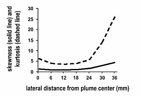
Skewness and kurtosis close to the plume axis are close to the values expected for a normal

Gaussian distribution, zero and 4 respectively. However, at the edges of the plume distributions become

leptokurtic and skewed toward higher values (Fig. 10).

3.4 INTERMITTENCY

Intermittency in the axial center of continuous and oscillatory plumes is low, but greater than zero, and

increases toward the plume edge (Fig. 11). The across-plume profiles vary with distance downstream.

Close to the source, the profile tends to be flat with a large core of intermittency values near zero, which

then increases toward the plume edge to values near 1.0. However, downstream the profile shows a

systematic increase in intermittency from the axis to the edge.

Moreover, for all the plumes, the measured intermittency at the centerline increased with

distance from the source (Fig. 12). The continuous and oscillatory plumes showed systematic increases

with distance downstream, but the continuous plume’s centerline intermittency reaches its peak at 200

mm. The largest changes in intermittency with consecutive downstream distances were observed in the

oscillatory plume. For the pulsed plumes, however, the increase was not evident until 400 mm from the

source. For both continuous and oscillatory plumes the intermittency seems to plateau at about 0.6 at 200

mm downstream of the source. This is lower than the values found by Murlis and Jones [8] and Jones [9]

in field measurements, which are about 0.8 at a roughly equivalent distance, but within the range of

values (0.4 to 0.8) in wind tunnel measurements of Fackrell and Robins [12]. The field measurements can

be expected to give higher intermittency due to the effects of undulation and meandering. Fackrell and

Robins found a very significant effect of source size on intermittency: our measurements compare well

with their measurements from a source of approximately 15 mm. Fackrell and Robins used a wind tunnel

speed of 4 m s-1 but even so, their results suggest that that our effective source size may not be well

characterized by a value based on the bore of the pipettes (1 mm).

14

3.5 PEAK-TO-CONDITIONAL-MEAN RATIOS

One of the main characteristics of a fluctuating signal is that there is a considerable contrast between

peak amplitudes and the mean. In these concentration signals, the peak-to-mean ratio has been estimated

as a ratio of the highest value registered in a sample to the overall sample mean and, to eliminate the

influence of intermittency, to the conditional mean. Peak-to-mean and peak-to-conditional-mean ratios

were similar, but because the overall means of the pulsed plumes are dominated by intermittency due to

pulsing, only the peak-to-conditional-mean ratios can be interpreted. Measured peak-to-conditional-

mean ratios averaged over an ensemble of samples from the 12 mm by 12 mm core of each plume type

are shown in Fig. 13. Peak-to-conditional-mean ratios for the continuous plume show no significant

trend with distance from the source at values of approximately 4.2. For the oscillatory plume, ratios are

significantly lower (P < 0.05) furthest downstream with no significant differences at distances of 50, 100,

and 200 mm from the source with values of about 4. The corresponding peak concentration to overall

mean concentration ratios, which is about 10 to 15, are lower than values reported in field trials [8, 9, 25]

which are in the range 20 to 30 and this could be due to the impacts of meandering and undulation on the

overall mean. In both these cases, the peak to conditional mean ratios fell less steeply with downstream

distance than conditional mean, suggesting that peaks in the signal become less marked closer to the

source. In both vertical and horizontal plumes, ratios were significantly greater (P < 0.05) nearest the

source than at 400 mm downstream, but each showed different patterns. Peak to mean ratios in the

horizontal plume declined systematically from approximately 7, leveling off at 200 mm downstream at

about 3.5, whereas the vertical plume at 100 and 200 mm downstream shows similar intermediate ratios

of about 3.8. The ratios of the continuous and oscillatory plumes close to source differ from those of the

pulsed plumes, and it is possible that the higher peak to conditional mean ratios in the pulsed plumes

arise from deviations in the form of the pulses from the ideal “square waveform”.

3.6 BURST LENGTHS

Intermittency is a useful measure of the average time-dependant structure of a signal, but loses the details

of the fine-scale structure. A signal of a given intermittency could be comprised of a few long, well-

separated bursts or of many closely packed bursts. The burst length is of biological interest because

many odor sensors adapt when exposed to a stimulus for any length of time (see [26] for a discussion of

adaptation).

15

On the plume edge where the signal is highly intermittent (that is, there are significant periods

when the concentration is less than 1 ppm), we generally expect to see the shortest burst lengths and the

highest mean interval between bursts. Correspondingly, the total number of burst events will diminish

toward the plume edge as fewer and fewer peaks in the signal achieve levels above the threshold. A

rather different type of behavior is displayed on the plume axis where there are few occasions when the

signal falls below the discrimination threshold and only a small variation in concentration occurs over the

entire record.

During these trials, pulses generated were 20 ms in duration. However, the measured burst

lengths suggested that the pulses produced contained internal structure with bursts of shorter lengths,

which expanded initially as they moved down the tunnel before diminishing downstream (Fig. 14a). The

burst lengths in the continuous plume were significantly greater (P < 0.05) at 50 mm from the source

(about 2 seconds) than at 200 and 400 mm from the source (about 0.5 seconds) and, although not

significant, a similar trend in the oscillatory plume was observed with burst lengths in a range 0.3 to 0.7

seconds (Fig. 14b). These mean burst lengths are long compared to those measured in the field [8, 9],

which are of the order of 0.2 seconds. However, the field measurments are heavily influenced by large-

scale movements of the plume. In terms of length scale, there is closer agreement with tunnel bursts

associated with length scales of 150 - 350 mm and bursts in the field with mean lengths of about 400 mm.

3.7 FREQUENCY SPECTRUM OF CONCENTRATION FLUCTUATIONS

The Fourier analysis of the pulsed plume signal was dominated by the pulse emission rate of 10

Hz (Fig. 15)]. For the continuous and oscillatory plumes, however, spectral density plots show a more

widely distributed spectrum with strong contributions from frequencies below 5 Hz, particularly closer to

the source (Fig. 15). The corresponding periods for the spectral peaks, 200 ms at 5 Hz and 100 ms at 10

Hz, are large compared to the burst lengths measured, which are tens of ms in length. Moreover, the

dominant frequencies in the spectrum change with position along the tunnel. For example, Fourier

analysis of the oscillatory plume at 100 mm from the source shows strong peaks at 0.4, 1.9, and 3.2 (Fig.

15d) but at 400 mm downstream from the source, peaks are observed at 1.0, 3.7, 4.1, and 5.2 (Fig. 15e).

In these trials a circular paper disk was used to generate turbulence. Air spilling over the disk in

an arrangement of this kind produces a series of vortices shed from alternate sides of the disk with a

characteristic frequency. The non-dimensional form of this frequency is the Strouhal number (see for

example, Vogel [27]), calculated as St = nl/U, where n is the frequency of the periodically varying flow,

16

l is a transverse dimension, and U is the fluid velocity. In the case of our oscillatory plume at 100 mm

downstream from the source, there are strong frequency contents at 1.9 Hz and 3.2 Hz, giving St = 0.133

and 0.224, respectively. These values are typical of those found respectively for long flat plates and

circular cylinders set laterally to the flow.

4. Discussion

The principal motivation for these trials was the need to characterize the stimulus available to

insects flying along airborne odor plumes. The ultimate aim was to measure the structure of surrogate

odor plumes in a wind tunnel so that the principal features could be related to behavioral maneuvers of

male moths flying along pheromone plumes of the same form. This would provide a working guide for

future studies and a means of interpreting differences in behavior seen in previous work. Although there

is an abundance of laboratory studies of insect navigation, to date, relatively little work has been reported

on the structure of the air-borne plumes along which these insects orient, other than time-averaged, plume

boundaries. Therefore, interpretations of behavior have been based mainly on output (i.e., flight

characteristics) rather than input-output (i.e., what instantaneous signal is intercepted by the animal and

the resultant flight patterns).

Previous studies have shown demonstrable effects of plume structure on the flight path of moths.

Mafra-Neto and Cardé [1] reported flight tracks (mean track angles of 41.5º ± 12.1) more toward upwind

(0º) in a turbulent plume (similar to the oscillatory plume presented here) and plumes pulsed at 5 per

second produced similar flight tracks (mean track angles of 40.4º ±14.0). However, slowly pulsed

plumes of < 1 per second produced flight tracks with more crosswind headings (73.9º ±7.2). Similarly,

male gypsy moths produced tracks of slower ground speed and greater track angles in plumes from a

point source compared with a more diffuse plume from a cylindrical baffle [28]. Furthermore, flight

behaviors, such as ground speed and track angle, change as an insect approaches an odor source [19, 22,

23], suggesting that plume characteristics evoke specific behaviors and that changes in plume

characteristics induce alterations in flight behaviors.

A further problem is that of replicating in laboratory conditions the pattern of odor stimulus and

wind found in the field and described in, for example, Murlis and Jones, [8] and Murlis et al. [25]. The

main difference between the conditions in the laboratory and the field is that, in wind tunnels, the scale

of turbulence is severely constrained so that the plume neither meanders nor undulates and the intensity

of large-scale fluctuations in wind speed is considerably diminished. The magnitude of concentration of

17

the chemical stimulus in these wind tunnel trials is designed to be of a similar level to that found in the

field and the intensity of fluctuations appears not to be enormously different from the levels described in

the field by Mylne and Mason [10]. The mechanical forces acting on the flying insect, however, due to

turbulent fluctuations in wind speed and direction, are far less in wind tunnels.

For more than 50 years, flight tunnels of the kind we describe, have been used in entomological

investigations of the behavioral roles of particular odorants, response profiles to individual components

or ratios of blends, sensory adaptation, habituation, and disruption, and mechanisms of orientation (see

[18]). Laboratory flight tunnels are generally rectangular or arch-shaped in cross-section and rarely

longer than 2 m. The ends of the tunnel are usually capped with window screening or cheesecloth to

contain flying insects and, at the upstream end, to reduce the level of turbulence in the airflow.

Characterizing the flow has typically been through the use of visual markers, such as cigarette or TiCl4

‘smoke’. Although these markers are useful to define roughly the time-averaged boundaries of a plume

and to give a qualitative understanding of structure, they are not strictly passive and it is difficult to make

quantitative measures of plume structure using them. To date, instantaneous plume structures of

pheromone plumes have not been described in sufficient detail to allow comparison with the subtle

changes seen in the flight maneuvers of insects. In particular, differences in the fine-scale features of the

plume near the source where the flow is not fully developed, have not been explored, although changes in

flight behaviors in this region have been observed in insect studies [19, 22, 23]. In this paper we describe

the differences in the forms of signals taken from plumes in their initial stages in these flow regimes and

suggest ways in which these signals could modulate the insect’s flight response. The results reflect the

real conditions in which flight trials are carried out in laboratories, and we believe that this analysis

provides insights into the signals insects typically encounter in work of this kind.

Usually, the plumes used in entomological studies are generated from a pulsing apparatus (pulsed

plume), a point source such as a filter paper impregnated with a volatile odorant (continuous plume), or a

continuous plume source with a disturbance in flow (oscillatory plume), and each of these elicit distinct

patterns of flight (Fig. 1). Flight tracks in pulsed and oscillatory plumes tend to be straighter than flight

tracks in continuous plumes. Flight tracks in pulsed plumes can resemble more closely either those in

continuous or oscillatory plumes, depending on the pulsing rate (crosswind flight occurs at low pulse

rates) and plume diameter (animals tend to exit small diameter plumes frequently). Here, we have

measured the fine-scale features of each of these plume types and note that certain features are distinctly

different in the different plume types. For example, absolute average concentrations in the plume

centerline are three to five times higher in the continuous plume than either of our pulsed plumes, and

oscillatory plumes about half that of the continuous plumes. Mean burst lengths follow a similar pattern

18

with the continuous plume showing longer bursts, at least near the source, and the oscillatory plume

producing short bursts similar to the pulsed plumes.

There are three plume properties that vary systematically with distance from source during the

initial stages of plume development and which may play a role in mediating the flight behaviors of

insects as they approach a source. They are mean concentration, intermittency, and in the case of

continuous and oscillatory plumes, intensity of concentration fluctuation. There may be other features of

the plume that play a role in orientation.

In each of the flow regimes the signal is intermittent and fluctuates in strength. Where the tracer

source is pulsed, artificially introduced intermittency dominates over the length of the plume. In this

case the pulse length, initially 20 ms, matches typical burst lengths measured in the field [25]. In

addition, the periods of inactive signal of the continuous and oscillatory plumes were broadly within the

ranges of burst return periods found in intense periods of bursts measured in the field, although they did

not vary as much as would be the case in the field [25]. An inspection of the signal in the continuous

plume (Fig. 7) suggests that a fixed sensor in it would register greater intermittency than it would in the

oscillatory plume (Fig. 6), with fewer bursts and shorter burst lengths and correspondingly shorter

intervals between bursts. The plume width, about 30 mm, was of a sufficient scale to engulf insects of

the species typically used in the flight trials. However, insects often carry out counterturning maneuvers

yielding a zigzag flight path, which can readily take them outside of the time-average boundaries of the

plume. Such lateral excursions would affect their perception of intermittency and flux in the signal they

encounter.

In flight trials, the number of excursions made by male almond moths, Cadra cautella, across the

centerline of a pheromone plume was 3-5 per second [14], and that of male gypsy moths, Lymantria

dispar, was 3-4 per second [20]. Furthermore, an animal maneuvering along a plume’s edge alters its

perception of the plume such that it encounters a fluctuating signal. Edge-following behaviors have been

observed in the moths Adoxophyes orana [3, 4], and Grapholita molesta [29], and in the blue crab,

Callinectes sapidus [30], and the copepod, Temora longicornis [31]. Following an edge or boundary

provides an animal with a series of on-off signals. In these cases where the animal exits the boundaries

of the plume, perceived intermittency would be higher than the actual intermittency in the plume; that is,

less time is spent in signal above threshold. Whether or not an insect maintains a due upwind heading or

zigzags off the wind-line, alters potential, real-time actuation by its receptors. The intermittency

recorded by a stationary sensor within the plume, therefore, underestimates the realized intermittency of

a moving insect counterturning upwind through the plume. The oscillatory plume described here is

roughly twice the diameter of the continuous plume and grows more rapidly as it advances downstream.

19

At this size, the plume would engulf the insects, during all but the most extreme lateral movements. The

well-mixed internal structure of this plume contains slightly shorter burst lengths and lower intermittency

but large differences in concentration compared to the continuous plume. Such a plume is likely to

provide a signal with a more constant stimulus and a lower mean concentration, a consequence of which

could be sensory cell adaptation.

We have treated estimates of intermittency with caution because intermittency is dependent on

the discrimination threshold set. As threshold increases, intermittency values will become large,

eventually reaching a value of 1, where the threshold exceeds the peaks of odor bursts in the signal. In

these trials, the threshold is fixed, but in the case of a biological sensor (i.e., a flying moth), threshold

will vary with adaptation events (where threshold increases) and with either disadaptation or sensitization

events (where threshold decreases).

Similarly burst length is dependent on threshold set; burst lengths decrease as threshold

increases. With our static sensor and a threshold of 1 ppm, burst lengths of the continuous plume

decreased with distance from source. Such relative changes that correlate to distance from source may

influence the flight track of a moth orienting along such a plume, and changes in flight behaviors of

moths approaching a source have been reported. For example, Willis et al. [32] found that flight tracks

of gypsy moths were narrower and ground speeds decreased closer to a point source in the field. An

insect that flies rapidly through long bursts and slower through short bursts, encounters a less variable

burst length, but its experience of the rate of onset of that signal is also altered.

Another feature of the odor signal that has been proposed as a behavioral cue, is the rapid rise in

concentration at the leading edge of bursts. Atema [33] noted systematic changes with distance from

source in the rate of rise in concentration at the leading edge of bursts and suggested that this formed part

of the information used by lobsters, Homarus americanus, walking up a flume to a source of food odor.

This is an explicitly chemotactic mechanism. It does not rely on rheotaxis, orientation to the direction of

current flow, but instead, depends directly on changes in the physical structure of the plume, in this case,

the rise in concentration at the leading edge of bursts, to regulate upstream maneuvers. Whether flying

moths use the rapid rise in concentration at the leading edge of bursts is currently unknown. Webster and

Weissburg [34] found that blue crabs did not appear to have the ability to resolve the slope a leading edge

of a concentration burst. Bursts observed in recordings by our stationary miniPID (e.g. Figs. 5, 6, and 7)

show very rapid burst activity with steeply sloped leading and trailing edges. It seems unlikely that

moths would have ability to resolve these temporal characteristics, given that response rates of projection

neurons in the central nervous system of those moths studied seem to be limited to 10 Hz or so [17, 24]

20

Over the range of source-to-sensor distances examined in this study, peak-to-conditional-mean

ratios decrease with distance from the source in pulsed plumes, are unchanged in the continuous plume,

and show no trend in the oscillatory plume. Interestingly, a plume type that is used often in insect

orientation studies – a ‘turbulent plume’ within a laminar flow, (e.g. [14, 35]), described here as an

oscillatory plume – is also the plume type that shows no trend in peak-to-conditional mean ratios with

downstream distance from source. The variability of this parameter suggests that it is not a reliable one

for predicting distance to source. Furthermore, as we have stated for steeply sloped edges of bursts,

moths appear to possess a neuronal resolution an order of magnitude lower than would be required to

sufficiently resolve peak-to-conditional mean ratios. Therefore, peak-to-mean ratios are not likely to be

involved in orientation of flying moths.

Although Fourier analysis unveiled some periodicities of low frequency in the continuous and

oscillatory plumes, it seems unlikely that the periodic nature of the signal per se is important to a male

moth orienting along a pheromone plume but rather the presence of a sufficient number of filaments per

second presented to the insect ensures that the animal continues upwind progress rather than ‘casting’

without progressing upwind [1, 14, 15]. Periodicities of the oscillatory and continuous plumes changed

with tunnel position, exhibiting larger frequencies further from the source. In fact, the rate of

interception of pulses has a considerable influence on flight maneuvers. Cadra cautella flies faster and

more toward upwind in pulsed plumes of ≥10 Hz than in plumes pulsed at ≤ 5Hz [15, 21]. The changes

exhibited in these maneuvers as an insect approaches a source, such as a decrease in flight speed [32],

could be due to these changes in the plume’s periodicity. Periodicity of concentration fluctuations in

oscillatory plumes in flight tunnels has not previously been described.

The present measurements made in the kinds of plume types routinely employed in studies of

moth orientation to pheromone ([21], et ante) confirm that structural features of these plume types differ,

and that these features change systematically within 100 to 400 mm of the upstream sources of odor.

These characteristics are candidate cues for the observed changes in flight maneuvers as male moths

approach pheromone sources. Among the behavioral changes typically observed are a decrease in

velocity along the track and a narrowing of the track’s lateral extent [19, 22, 23, 32]. Such changes are

often a prelude to landing near (or sometimes on) the odor source. Because of intermingling effects of

dynamic thresholds, sensory cell adaptation, counterturning in freely-flying animals, and temporal scales

of resolution unique to biological systems, we suggest that the rate in rise of concentration at the leading

edge of bursts, peak-to-mean ratios, and periodicity are not used by male moths in locating pheromone

sources. In addition, we suggest that intermittency is not used by male moths to distinguish ‘near’ or

‘far’ from a plume’s source, but rather that an intermittent plume is required to sustain upwind progress.

21

We suggest that the flight track is shaped by a combination of absolute concentration and burst length,

and that as a moth approaches a source, concurrent changes in concentration and filament interception

rate may induce changes in flight behaviors.

5. Acknowledgement

We thank Drs. E.A. Cowen and M.J. Weissburg, and two anonymous reviewers, for helpful comments on

this manuscript. We are grateful to Dr. J. Bau for performing Fourier analyses, and to Mr. D. Giles and

Mr. P. Stovall, College of Engineering at the University of California, Riverside, for the design and

fabrication of the x,y,z-traverse,. The research was supported by a grant from the Office of Naval

Research (ONR N00014-98-1-0820) under the ONR/DARPA Chemical Plume Tracing Program.

22

Fig. 1. Flight tracks of male Cadra cautella in three different plume types. Flight tracks displayed are ina region approximately 200-700 mm from the source. Pulsed plume: generated by an electronic pulsingapparatus and introduced to the wind tunnel through a horizontal rake of four pipettes, each containing apheromone-laden filter paper disk, release velocity was isokinetic with wind tunnel airflow (see [21]).Continuous plume: issuing from four pipettes, each containing pheromone-laden filter paper disk, and acontinuous airflow of 2.5 mL s-1, released as a jet (see [21]). Oscillatory plume: issuing from apheromone-impregnated filter paper disk mounted on a copper wire with a 30 by 30 mm plastic deflector40 mm downstream of the filter paper disk (see [14], reproduced with permission). Tick marks on theabscissa are each 100 mm. Each dot represents the position of the moth every other frame: 0.067 s fortracks in the pulsed and continuous plume; 0.033 s for the track in the turbulent plume. Track angles andairspeeds reported are means of all flight tracks of animals in those conditions. (See [21] for behavior ofmoths in pulsed and continuous plumes; see [14] for behavior of moths in oscillatory plumes.)

Fig. 2. A 3-m long wind tunnel typical of entomological studies, constructed with Lexan® andPlexiglas®. The upwind end has a 150-mm deep block of aluminum Hexcel® to laminize airflow.Window screening covers both the upwind (not shown) and downwind ends of the tunnel. A cowling ofpolyvinyl sheeting attaches the downwind end to an exhaust duct (not shown). Openings in the side ofthe tunnel are sealed with polyvinyl sheeting to minimize the disturbance in airflow during experiments.

Fig. 3. Orthogonal wind components, U, V, and W, in a wind tunnel sampled at 60 Hz with a 3-D sonicanemometer. (a) wind speed in the tunnel, (b) intensity of fluctuations in the streamwise velocity, (c)intensity of fluctuations in the lateral component of velocity parallel to the wind tunnel floor, and (d)intensity of fluctuations in the vertical component of velocity.

Fig. 4. Odor sources issuing from modified Pasteur pipettes. (a) A linear array of four pipettes (notdrawn to scale) were set ~18 mm apart. Airflow (2.5 ml s-1) from each of two pulse generator outlets wassplit to two pipettes via polyvinyl tubing; (b) the linear array was set either horizontally, as shown, orvertically; arrow denotes wind direction in the flight tunnel; (c) a continuous point source released intoan oscillatory flow was produced by placing a 35 mm circular paper disk (shown as a black line) ~ 25mm upstream of a modified Pasteur pipette via copper wire (shown as gray line); arrow denotes winddirection in the flight tunnel.

Fig. 5. Representative traces at the axial center of one of the odor sources of the vertical pulsed plumeusing a miniature photoionization detector (miniPID) at four distances downstream of the odor source:(a) 50 mm, (b) 100 mm, (c) 200 mm and (d) 400 mm. Each trace is 15 s.

Fig. 6. Representative traces from the axial center of the oscillatory plume using a miniaturephotoionization detector (miniPID) at four distances downstream of the odor source: (a) 50 mm, (b) 100mm, (c) 200 mm and (d) 400 mm. Each trace is 15 s.

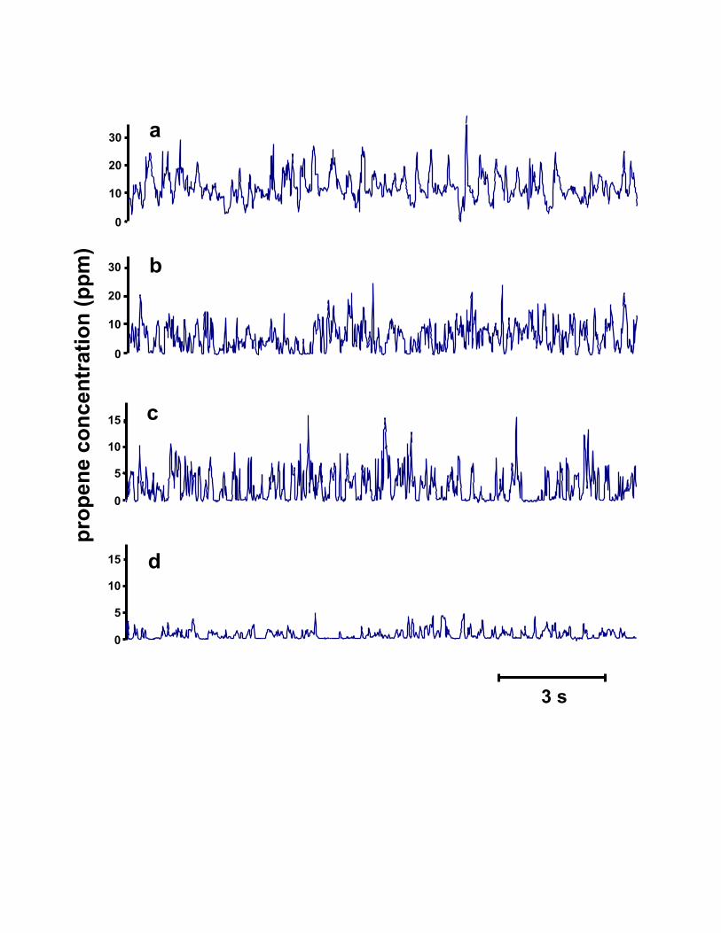
Fig. 7. Representative traces from the axial center of the continuous plume using a miniaturephotoionization detector (miniPID) at four distances downstream of the odor source: (a) 50 mm, (b) 100mm, (c) 200 mm and (d) 400 mm. Each trace is 15 s.

Fig. 8. Conditional mean concentrations (± standard error) averaged over the center 12 mm by 12 mmcore of each plume type relative to source concentration at four distances downstream of the odor source.The conditional mean is the mean formed during periods of active signal, rejecting regions of below-threshold signal.

23

Fig. 9. Intensity of concentration fluctuation (± standard error) estimated for each ‘x’ position from thelinearized approximation to the relationship between mean concentration and standard deviation. Notethat pulsed plumes do not vary much with downstream distance, but that continuous and oscillatoryplumes have ratios that more than double downstream.

Fig. 10. Higher moments of concentration fluctuations: skewness and kurtosis of the oscillatory plume100 mm downstream from the source. Values reported are from recordings at the plume’s axial center,‘0’, moving outward toward the lateral edge.

Fig. 11. Intermittency values, 1 – γ, across the (a) continuous and (b) oscillatory plumes at twodownstream distances, 50 and 400 mm, from the source. Values reported are from recordings at theplume’s axial center, ‘0’, moving outward toward the lateral edge.

Fig. 12. Intermittency values, 1 – γ, (± standard error) averaged over the center 12 mm by 12 mm core ofeach plume type at four distances downstream of the odor source.

Fig. 13. Peak-to-conditional-mean ratios (± standard error) of each plume type at four distancesdownstream of the source.

Fig. 14. Mean length of bursts (± standard error) recorded at the center 12 by 12 mm core of each plumetype at four distances downstream of the odor source.

Fig. 15. Spectral density plots of the (a) vertical pulsed, (b and c) continuous, and (d and e) oscillatoryplumes. Measurements were made at (a, b, and d) 100 mm and (c and e) 400 mm from the odor source.Peaks are evident at 10 Hz in the pulsed plume; the continuous and oscillatory plumes show severalfrequencies, and in both plume types, frequencies get larger with distance downstream.

24

6. Literature Cited

1. Mafra-Neto, A. and Cardé, R.T.: 1994, Fine-scale structure of pheromone plumes modulates upwindorientation of flying moths, Nature, 369, 142-144.

2. Vickers, N.J. and Baker, T.C.: 1994, Reiterative responses to single strands of odor promote sustainedupwind flight and odor source location by moths Proc. Nat. Acad. Sci. U. S. A., 91, 5756-5760.

3. Kennedy, J.S., Ludlow, A.R. and Sanders, C.J.: 1980, Guidance system used in moth sex attraction,Nature, 288, 475-477.

4. Kennedy, J.S., Ludlow, A.R.and Sanders, C.J.: 1981, Guidance of flying male moths by wind-bornesex pheromone, Physiol. Entomol., 6, 395-412.

5. Geier, M., Bosch, O.J. and Boeckh, J.: 1999, Influence of odour plume structure on upwind flight ofmosquitoes towards hosts, J. Exp. Biol., 202, 1639-1648.

6. Dekker, T., Takken, W. and Cardé, R.T.: 2001, Structure of host-odour plumes influences catch ofAnopheles gambiae s.s. and Aedes aegypti in a dual-choice olfactometer, Physiol. Entomol., 26,124-134.

7. Kennedy, J.S. and Marsh, D.: 1974, Pheromone-regulated anemotaxis in flying moths, Science, 184,999-1001.

8. Murlis, J. and Jones, C.D.: 1981, Fine-scale structure of odour plumes in relation to insect orientationto distant pheromone and other attractant sources. Physiol. Entomol., 6, 71-86.

9. Jones, C.D.: 1983, On the structure of instantaneous plumes in the atmosphere, J. Hazard. Mater., 7,87-112.

10. Mylne, K.R. and Mason, P.J.: 1991, Concentration fluctuation measurements in a dispersing plume ata range of up to 1000 m, Q.J.R. Meteorol. Soc., 117, 177-206.

11. Yee, E., Chan, R., Kosteniuk, P.R., Chandler, G.M., Biltoft, C.A. and Bowers, J.F.: 1994,Experimental measurements of concentration fluctuations and scales in a dispersing plume in theatmospheric surface layer obtained using a very fast-response concentration detector. J. Appl.Meteorol., 33, 996-1016.

12. Fackrell, J.E. and Robins, A.G.: 1982, The effect of source size on concentration fluctuations inplumes. Boundary-Layer Meteorol., 22, 335-350.

13. Fackrell, J.E. and Robins, A.G.: 1982, Concentration fluctuations and fluxes in plumes from pointsources in a turbulent boundary layer, J. Fluid Mech., 117: 1-26.

14. Mafra-Neto, A. and Cardé, R.T.: 1995, Influence of plume structure and pheromone concentration onupwind flight of Cadra cautella males, Physiol. Entomol., 20, 117-133.

25

15. Mafra-Neto, A. and Cardé, R.T.: 1995, Effect of the fine-scale structure of pheromone plumes: pulsefrequency modulates activation and upwind flight of almond moth males. Physiol. Entomol., 20,229-242.

16. Vickers, N.J. and Baker, T.C.: 1996, Latencies of behavioral response to interception of filaments ofsex pheromone and clean air influence flight track shape in Heliothis virescens (F.) males, J.Comp. Physiol. A., 178, 831-847.

17. Vickers, N.J., Christensen, T.A., Baker, T.C. and Hildebrand, J.G.: 2001, Odour-plume dynamicsinfluence the brain’s olfactory code, Nature, 410, 466-470.

18. Baker, T.C. and Linn, Jr., C.E. 1984, Wind tunnels in pheromone research. In: Techniques inpheromone research, H.E. Hummel & T.A. Miller (eds.), pp. 75-110, Springer-Verlag, NewYork.

19. Willis, M.A. and Baker, T.C.: 1994, Behaviour of flying oriental fruit moth males during approach tosex pheromone sources, Physiol. Entomol., 19, 61-69.

20. Cardé, R.T. and Knols, B.G.L.: 2000, Effects of light levels and plume structure on the orientationmanoeuvres of male gypsy moths flying along pheromone plumes, Physiol. Entomol., 25, 141-150.

21. Justus, K.A., Schofield, S.W., Murlis, J. and Cardé, R.T.: 2002, Flight behaviour of Cadra cautellamales in rapidly pulsed pheromone plumes. Physiol. Entomol. (in press).

22. Murlis, J. and Bettany, B.W.: 1977, Night flight towards a sex pheromone source by male Spodopteralittoralis (Boisd.) (Lepidoptera, Noctuidae). Nature, 268, 433-435.

23. Murlis, J., Bettany, B.W., Kelley, J. and Martin, L.: 1982, The analysis of flight paths of maleEgyptian cotton leafworm moths, Spodoptera littoralis, to a sex pheromone source in the field.Physiol. Entomol., 7, 435-441.

24. Christensen, T.A. and Hildebrand, J.G.: 1988, Frequency coding by central olfactory neurons in thesphinx moth Manduca sexta, Chem. Senses, 13, 123-130.

25. Murlis, J., Willis, M.A. and Cardé, R.T.: 2000, Spatial and temporal structures of pheromoneplumes in fields and forests, Physiol. Entomol., 25, 211-222.

26. Bartell, R.J.: 1982, Mechanisms of communication disruption by pheromone in the control ofLepidoptera: a review, Physiol. Entomol., 7, 353-364.

27. Vogel, S.: 1981, Life in Moving Fluids: The Physical Biology of Flow, Princeton University Press,352 pp.

28. Willis, M.A., David, C.T., Murlis, J. and Cardé, R.T.: 1994, Effects of pheromone plume structureand visual stimuli on the pheromone-modulated upwind flight of male gypsy moths (Lymantriadispar) in a forest (Lepidoptera: Lymantriidae), J. Insect Behav., 7, 385-409.

26

29. Willis, M.A. and Baker, T.C.: 1984, Effects of intermittent and continuous pheromone stimulationon the flight behaviour of the oriental fruit moth, Grapholita molesta, Physiol. Entomol., 9, 341-358.

30. Weissburg, M.J., Dusenbery, D.B., Ishida, H., Janata, J., Keller, T., Roberts, P.J.W. and Webster,D.R.: 2002, A multidisciplinary study of spatial and temporal scales containing information inturbulent chemical plume tracking, Environ. Fluid Mechanics, (this issue).

31. Weissburg, M.J., Doall, M.H. and Yen, J.: 1998, Following the invisible trail: kinematic analysis ofmate-tracking in the copepod Temora longicornis, Phil. Trans. R. Soc. Lond B, 353, 701-712.

32. Willis, M.A., Murlis, J. and Cardé, R.T.: 1991, Pheromone-mediated upwind flight of male gypsymoths, Lymantria dispar, in a forest, Physiol. Entomol., 16, 507-521.

33. Atema, J.: 1996, Eddy chemotaxis and odor landscapes: exploration of nature with animal sensors,Biol. Bull., 191, 1129-138.

34. Webster, D.R. and Weissburg, M.J.: 2001, Chemosensory guidance cues in a turbulent chemical odorplume, Limnol. Oceanogr., 46, 1034-1047.

35. Marsh, D., Kennedy, J.S. and Ludlow, A.R.: 1978, An analysis of anemotactic zigzagging flight inmale moths stimulated by pheromone, Physiol. Entomol., 3, 221-240.

0

5

10

15

pro

pene

con

cent

ratio

n (p

pm)

a

b

c

0

5

10

15

0

10

20

30

0

10

20

30

3 s

d

prop

ene

conc

entr

atio

n (p

pm)

0

5

10

15 d

3 s

c

0

5

10

15

b

0

10

20

30

a

0

10

20

30

prop

ene

conc

entr

atio

n (p

pm)

0

15

30

45c

b

0

30

60

90

a

0

30

60

90

d

0

15

30

45

3 s