Embed Size (px)
Citation preview
REVISED TECHNICAL GUIDANCE ONHOW TO CONDUCT
EFFLUENT PLUME DELINEATION STUDIES
National Environmental Effects Monitoring OfficeNational Water Research Institute
Environment Canada
MARCH 2003
FINAL REPORT TO
ENVIRONMENT CANADA
ON
REVISED TECHNICAL GUIDANCE ON HOW TO CONDUCT EFFLUENT PLUME DELINEATION STUDIES
(CONTRACT NO. K1130-2-2033)
JACQUES WHITFORD ENVIRONMENT LIMITED711 WOODSTOCK ROAD
FREDERICTON, NB E3B 5N8Tel: (506) 366-1080Fax: (506) 452-7652
http://www.jacqueswhitford.com
AND
NATECH ENVIRONMENTAL SERVICES INC.109 PATTERSON ROAD
HARVEY STATION, NB E6K 1L9Tel: (506) 366-1080Fax: (506) 366-1090
http://www.natech.nb.ca
March 2003
Acknowledgements
This report was prepared by Mary Murdoch (Jacques Whitford Environment Limited (JWEL)), JochenSchroer (NATECH Environmental Services Inc. (NATECH)), and John Allen (NATECH). The JWEL –NATECH team are acknowledged for the technical and scientific expertise that they brought to thepreparation of this technical guidance. Special thanks are also extended to Mr. Roy Parker (EnvironmentCanada, Atlantic Region) who was the Scientific Authority for this project, and to the following peoplewho were members of the review team: Janice Boyd (Environment Canada, Pacific Region), Kay Kim(Environment Canada, Atlantic Region), Georgine Pastershank (National EEM Office, EnvironmentCanada), Bonna Jordan (National EEM Office, Environment Canada), Nardia Ali (Environment Canada,Ontario Region), and Debbie Audet (Environment Canada, Ontario Region).
Environment Canada Revised Technical Guidance for Effluent Plume DelineationPage i
TABLE OF CONTENTS
Page No.
1.0 INTRODUCTION ...........................................................................................................................11.1 Purpose of Plume Delineation .............................................................................................1
2.0 EFFLUENT DISPERSION .............................................................................................................32.1 Initial Concept of Effluent Dispersion.................................................................................32.2 Effluent Characteristics........................................................................................................52.3 Effluent Discharge Design...................................................................................................62.4 Receiving Environment Factors Affecting Plume Dispersion.............................................6
2.4.1 Freshwater Flows .....................................................................................................62.4.2 Water Levels ............................................................................................................72.4.3 Water Quality...........................................................................................................72.4.4 Variation in Temperature and Salinity.....................................................................72.4.5 Tides and Seiches.....................................................................................................72.4.6 Climatic Conditions .................................................................................................72.4.7 Confounding Conditions..........................................................................................8
3.0 FIELD TRACER STUDY ...............................................................................................................93.1 Study Team Personnel .........................................................................................................93.2 Communication....................................................................................................................93.3 Boats ..................................................................................................................................103.4 Positioning (GPS) ..............................................................................................................103.5 Tracer Selection .................................................................................................................103.6 Tracer Injection (Added Tracer) ........................................................................................11
3.6.1 Duration of Dye Injection ......................................................................................133.7 Water Quality Meters.........................................................................................................13
3.7.1 Fluorometer............................................................................................................133.8 Equipment Used to Track Currents and Effluent Movement ............................................15
3.8.1 Drogues ..................................................................................................................153.8.2 Current Meters .......................................................................................................16
3.9 Tracking Effluent Dispersion.............................................................................................173.9.1 Sampling in the Initial Dilution Zone ....................................................................173.9.2 Subsequent Dispersion...........................................................................................18
3.10 Data Quality .......................................................................................................................193.11 Numerical Modeling ..........................................................................................................20
4.0 REPORTING .................................................................................................................................22
5.0 RECEIVING ENVIRONMENT – SPECIFIC CONSIDERATIONS...........................................235.1 Rivers .................................................................................................................................23
TABLE OF CONTENTS (CONTINUED)
Page No.
Environment Canada Revised Technical Guidance for Effluent Plume DelineationPage ii
5.2 Small Lakes and Impoundments........................................................................................245.3 Large Lakes........................................................................................................................265.4 Estuaries and Fjords...........................................................................................................26
5.4.1 Hydrographic Considerations ................................................................................265.4.2 Conducting the Field Work....................................................................................31
5.5 Marine ................................................................................................................................325.6 Climatic Conditions ...........................................................................................................33
5.6.1 Ice...........................................................................................................................335.6.2 Wind.......................................................................................................................34
6.0 REFERENCES ..............................................................................................................................35
LIST OF TABLES
Page No.Table 3.1 Study Team Roles and Responsibilities...............................................................................9Table 3.2 Numerical Models for Describing Effluent Dispersion .....................................................21Table 5.1 Summary of factors to be considered for each type of receiving environment .................23
LIST OF FIGURES
Page No.Figure 2.1 Examples of plume behaviour in receiving environments (modified from Jirka et
al. 1996) ..............................................................................................................................5Figure 3.1 Typical calibration curve relating fluorescence to tracer dye concentration .....................14Figure 3.2 A variety of drogue types used for plume delineation (adapted from the Canadian
Tidal Manual) ....................................................................................................................15Figure 5.1 Generalized Profile of an Estuary, Showing Circulation During Ebb Tide (a) and
Flood Tide (b). ...................................................................................................................27Figure 5.2 Profiles of typical estuarine water masses, showing an highly stratified estuary
(a), a partially mixed estuary (b), and a fully mixed estuary (c)........................................28

Environment Canada Revised Technical Guidance for Effluent Plume DelineationPage 1
1.0 INTRODUCTION
At the request of Environment Canada (Contract No. K1130-2-2033), Jacques Whitford EnvironmentLimited (JWEL) and NATECH Environmental Services Inc. (NATECH) have prepared revisedtechnical guidance for pulp and paper effluent plume delineation for the aquatic environmental effectsmonitoring (EEM) required under the Pulp and Paper Effluent Regulations (PPER). This revisedguidance replaces the existing guidance for effluent plume delineation in Section 2.2 (“Description ofthe Study Area”) of the April 1998 release of the Pulp and Paper Technical Guidance Document forAquatic Environmental Effects Monitoring (Environment Canada 1998).
1.1 Purpose of Plume Delineation
Effluent plume delineation is required in the design phase of the EEM program for each pulp and papermill. The objective of plume delineation is to understand how the mill effluent behaves in the receivingenvironment and to identify effluent boundaries describing exposure areas and reference areas withinwhich to establish sampling locations.
The exposure area(s) for EEM studies is the area where the effluent concentration is 1% or greater,reflecting a dilution of no more than 1:100. It is important to understand the spatial distribution ofeffluent in the water column to determine areas for fish collection, as well as to understand where theeffluent comes in contact with the bottom substrate to determine areas for sampling the benthicinvertebrate community. This is particularly important for effluent that may not exhibit completevertical or horizontal mixing throughout the receiving environment.
Selection of sampling locations within the reference area(s) for EEM studies requires an understandingof the extended dilution of effluent beyond the 0.1% (1:1000 dilution) effluent concentration limit. Thisunderstanding is particularly important for mills discharging into water bodies where flow is notunidirectional.
Delineation of effluent plumes will typically involve field work to track plume movement during asingle time period, coupled with the use of numerical modeling to determine target dilution zones over abroader range of environmental conditions. It is recommended that the effluent exposure zone bepredicted for the:
• maximum extent, reflecting the zone within which effluent is periodically detectable at aconcentration of 1% or greater; and
• long-term average conditions, reflecting the zones within which effluent concentrations of 1% orgreater, and 0.1% or greater would be regularly detectable.
Environment Canada Revised Technical Guidance for Effluent Plume DelineationPage 2
Areas beyond the maximum extent delineation under worst case conditions would be expected to beminimally affected by the discharge and may be suitable as “far field” or “reference” areas, dependingon the sampling design (e.g., control/impact design or gradient design). The long-term averageconditions define what would be considered the “normal” envelop of plume extent and can be use todesign an EEM sampling program that will assess the long-term effect of the effluent discharge. It mayalso be useful to determine the long-term average conditions of 10% or greater effluent concentration toidentify areas that may be most impacted by exposure to effluent. It is important to evaluate what arethe “normal” environmental conditions to which the effluent will be subjected and what are the extremesthat may, on occasion, override the “normal”.
For discharge environments with high receiving water flow, in which the effluent is expected to berapidly mixed, it is important to determine whether the effluent is diluted to less than 1% within 250 mof the discharge, which would remove the EEM requirement to conduct a fish survey.
The EEM program requires that effluent plume delineation be conducted only once, provided there areno substantive changes in effluent characteristics, discharge quantity, discharge method or location, or inthe hydraulic or hydrographic features of the receiving environment. Plume delineation must bereviewed in the design phase of each subsequent cycle of EEM to evaluate the need for a newdelineation. The onus is on the mill to ensure that they have an understanding of the hydrographicnature of the receiving waters, sufficient data and numerical modeling to meet the objectives of plumedelineation for EEM.
Environment Canada Revised Technical Guidance for Effluent Plume DelineationPage 3
2.0 EFFLUENT DISPERSION
Plume delineation requires information on effluent characteristics, discharge conditions and the natureof the receiving environment.
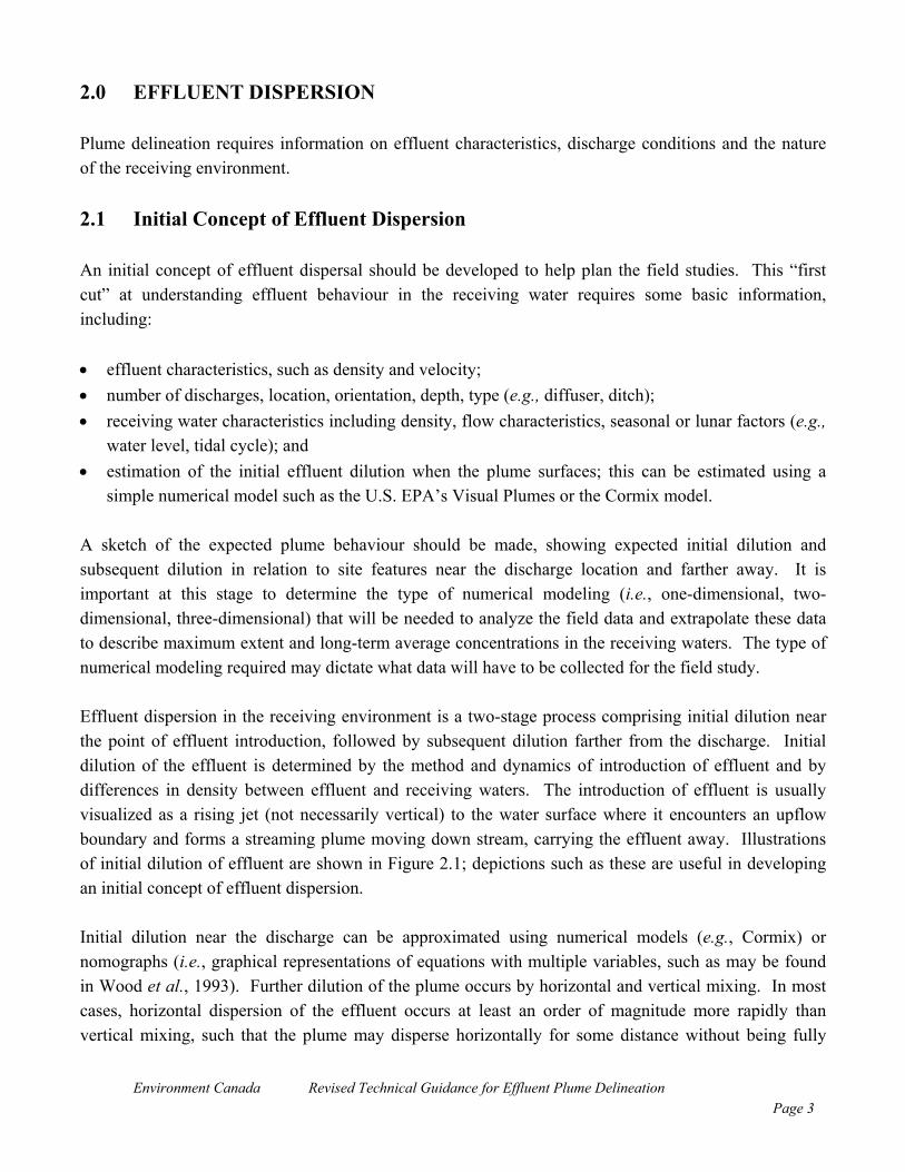
2.1 Initial Concept of Effluent Dispersion
An initial concept of effluent dispersal should be developed to help plan the field studies. This “firstcut” at understanding effluent behaviour in the receiving water requires some basic information,including:
• effluent characteristics, such as density and velocity;• number of discharges, location, orientation, depth, type (e.g., diffuser, ditch); • receiving water characteristics including density, flow characteristics, seasonal or lunar factors (e.g.,
water level, tidal cycle); and• estimation of the initial effluent dilution when the plume surfaces; this can be estimated using a
simple numerical model such as the U.S. EPA’s Visual Plumes or the Cormix model.
A sketch of the expected plume behaviour should be made, showing expected initial dilution andsubsequent dilution in relation to site features near the discharge location and farther away. It isimportant at this stage to determine the type of numerical modeling (i.e., one-dimensional, two-dimensional, three-dimensional) that will be needed to analyze the field data and extrapolate these datato describe maximum extent and long-term average concentrations in the receiving waters. The type ofnumerical modeling required may dictate what data will have to be collected for the field study.
Effluent dispersion in the receiving environment is a two-stage process comprising initial dilution nearthe point of effluent introduction, followed by subsequent dilution farther from the discharge. Initialdilution of the effluent is determined by the method and dynamics of introduction of effluent and bydifferences in density between effluent and receiving waters. The introduction of effluent is usuallyvisualized as a rising jet (not necessarily vertical) to the water surface where it encounters an upflowboundary and forms a streaming plume moving down stream, carrying the effluent away. Illustrationsof initial dilution of effluent are shown in Figure 2.1; depictions such as these are useful in developingan initial concept of effluent dispersion.
Initial dilution near the discharge can be approximated using numerical models (e.g., Cormix) ornomographs (i.e., graphical representations of equations with multiple variables, such as may be foundin Wood et al., 1993). Further dilution of the plume occurs by horizontal and vertical mixing. In mostcases, horizontal dispersion of the effluent occurs at least an order of magnitude more rapidly thanvertical mixing, such that the plume may disperse horizontally for some distance without being fully
Environment Canada Revised Technical Guidance for Effluent Plume DelineationPage 4
mixed in the water column. It is therefore important to consider the depth component of dispersionduring the field studies and to incorporate this into numerical modeling to determine the plume locationwithin the water column and where it comes into contact with the bottom substrate.
Discharged effluent usually has higher velocity than the receiving water, which results in shear stresswith the receiving water. This shear stress results in turbulent mixing. Initial dilution continues untilthe energy in the discharge dissipates and the velocity of the plume matches that of the receiving water.Once this occurs, the “natural” turbulence in the receiving water causes further dilution or mixing of theeffluent with the receiving water.
In addition to velocity differences, most receiving water and effluents differ in density. The effluent istypically less dense than the receiving water (often due to being warmer, or freshwater effluentdischarging to marine waters) and therefore tends to rise in the water column. This results in anothershear stress, similar to that resulting from the velocity difference.
In most cases, the combination of velocity and density shearing provides sufficient upward momentumto cause the effluent plume to break the water surface. If the density of the plume mixture is still lighterthan the receiving water, then the plume will stay at the surface. If the plume mixture is slightly heavierthan the receiving water, it will plunge down to the level at which there is a water mass of equal densityand then be transported by and mix with that body of water.
After initial dilution, the effluent plume typically moves horizontally with the receiving waters.Subsequent dilution and dispersion depends on the receiving environment and climatic conditions (seeSection 2.4).
Additional resources for guidance on effluent dispersion conceptualization include: Bishop (1984), Day(1975), Jirka et al. (1996), Neshyba (1987), Roberts (1989), Roberts and Ferrier (1996), Sorensen(1978), Thomann and Mueller (1987), Tsanis and Valeo (1994), Williams (1985), and Wood (1993).

Figure 2.1 Examples of plume behaviour in receiving environments(modified from Jirka et al. 1996)
Environment Canada Revised Technical Guidance for Effluent Plume DelineationPage 6
2.2 Effluent Characteristics
The most important effluent characteristics that influence initial dispersion are density and velocitydifferences compared to receiving water (see Section 2.1). Velocity will influence the degree of shearand therefore mixing that occurs when effluent is discharged. Effluent density will influence the rate ofrise and position of the plume in the water column. Velocity may be measured as effluent flow rate (as adaily average), including whether the discharge is continuous or discontinuous (e.g., batch release). Thevelocity of flow through each discharge pipe port should be considered, in comparison to the receivingwater. Density of the effluent should be determined. Additional information on the effluent for plumedelineation may include the presence of tracers, which are substances occurring naturally in the effluent,such as resin acids, sodium, and magnesium. These tracers may be used to track dispersion. Effluentvalues for the two most recent years should be considered.
2.3 Effluent Discharge Design
The discharge configuration and performance should be described. Using existing data, such as themost recent underwater inspection reports of the discharge, the performance should be compared to thedesign or the “as built” drawings. The location, length and orientation of the discharge should be knownwhen determining the width of the plume. It is also important to consider the depth of the dischargewithin the water column in relation to flows and density gradients that may exist.
2.4 Receiving Environment Factors Affecting Plume Dispersion
The receiving environment should be described in terms of flow and currents, physical and chemicalwater quality and the spatial and temporal variations of these factors. This information is necessary todevelop an initial concept of effluent dispersion, as well as to plan the field study. Climatic conditionsshould be summarized, with a view to their possible influence on plume behaviour.
Field parameters and their general importance in delineating plumes are described below. More detailedguidance for specific receiving environments is provided in Section 5.
2.4.1 Freshwater Flows
Minimum, maximum and average freshwater flows should be described in the receiving environment.This is important for all receiving environments, except those that are strictly marine with no localfreshwater inputs. Freshwater flows will influence the initial dilution of the plume as well assubsequent horizontal and vertical mixing. The direction of flow, which may vary with depth andlocation, will influence the orientation of the plume. Typically, field studies are conducted at nearminimum annual flow when effluent dilution will be low and the plume large relative to other times of
Environment Canada Revised Technical Guidance for Effluent Plume DelineationPage 7
the year. Field results can be extrapolated to reflect average and maximum flow scenarios for effluentdispersion.
2.4.2 Water Levels
Minimum, maximum and average water levels should be described for all receiving environments. Thewater level will influence initial dilution and the volume of water available for subsequent dispersion.Fluctuations in water level may occur daily (i.e., tidal areas) or seasonally.
2.4.3 Water Quality
Water quality measures for receiving water that may be useful for plume delineation studies includetemperature, density or specific gravity, salinity (for estuarine and marine studies), colour, suspendedsolids, and substances that may be used as effluent tracers. All of these measures can be used to trackthe movement of effluent within the receiving environment, as described in Sections 3 and 5.
2.4.4 Variation in Temperature and Salinity
Temperature and salinity both affect the density of the receiving water, and therefore their structure andvariation within the water mass over space and time is important in all aspects of conducting a plumedelineation study. Plumes that are warmer or less saline than the receiving water will be thermallybuoyant when discharged and will rise towards the surface, creating shear that will generate initialmixing and dilution. Subsequent dilution and dispersion will also be influenced by temperature andsalinity in the receiving water. Temperature and salinity may vary horizontally and vertically over short(e.g., tidal areas) or long (e.g., seasonal) time frames.
2.4.5 Tides and Seiches
The timing of tides and magnitudes is important to understand when planning the field study forestuarine and marine waters. In addition to marine and estuarine receiving waters, large lakes may alsodisplay a tidal cycle, albeit minor by comparison. Large bodies of water, such as lakes, estuaries andfjords, may also display the effects of storm surges and seiches, both in the surface elevation and ininternal waves. All of these will influence the direction and pattern of effluent mixing.
2.4.6 Climatic Conditions
Wind and ice may significantly affect effluent dispersion, air temperature, ice conditions and waveaction can all influence plume behaviour. Wind acting on large bodies of water may induce currents andwaves. Ice may affect dispersion in two ways: by reducing wind-driven currents, and by increasing
Environment Canada Revised Technical Guidance for Effluent Plume DelineationPage 8
turbulence by providing a solid rough boundary to flow. Climatic conditions are discussed in moredetail in Section 5.
2.4.7 Confounding Conditions
Although plume delineation is intended to capture normal discharge and receiving environmentconditions, there are some potentially confounding conditions that may influence interpretation of fieldstudy results. Confounding conditions arise from events that are outside of the operational orenvironmental norms or are transitory events, and may result in a temporary change in the more“normal” location of plume boundaries. These conditions may affect effluent dispersion and therefore,their possibility should be considered when conducting a plume delineation study. Examples of suchconditions include the following:
• pulp mill system upsets in the effluent treatment and discharge process that result in a temporarychange in effluent quality or quantity;
• adverse weather, in particular wind conditions, that generates currents that are not typical for thereceiving environment;
• seasonal events, such as ice conditions or thermal stratification, which can lead to a misleadingrepresentation of the plume behaviour; and
• flow regulation for hydro-electric power production..
Environment Canada Revised Technical Guidance for Effluent Plume DelineationPage 9
3.0 FIELD TRACER STUDY
Field work involves tracking the dispersion of effluent using a tracer that is either naturally present inthe effluent or is added. The purpose of this study is to obtain sufficient field data on a “snap shot” ofeffluent dispersion such that numerical modeling can then be used to estimate the maximum extent ofthe ≥1% effluent plume, and the long term average extent of the ≥1% and the ≥0.1% effluent plumes.
3.1 Study Team Personnel
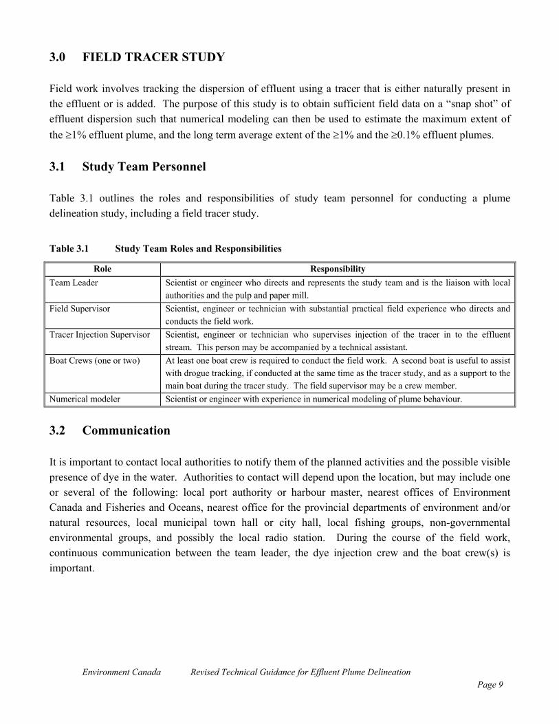
Table 3.1 outlines the roles and responsibilities of study team personnel for conducting a plumedelineation study, including a field tracer study.
Table 3.1 Study Team Roles and Responsibilities
Role ResponsibilityTeam Leader Scientist or engineer who directs and represents the study team and is the liaison with local
authorities and the pulp and paper mill.Field Supervisor Scientist, engineer or technician with substantial practical field experience who directs and
conducts the field work.Tracer Injection Supervisor Scientist, engineer or technician who supervises injection of the tracer in to the effluent
stream. This person may be accompanied by a technical assistant.Boat Crews (one or two) At least one boat crew is required to conduct the field work. A second boat is useful to assist
with drogue tracking, if conducted at the same time as the tracer study, and as a support to themain boat during the tracer study. The field supervisor may be a crew member.
Numerical modeler Scientist or engineer with experience in numerical modeling of plume behaviour.
3.2 Communication
It is important to contact local authorities to notify them of the planned activities and the possible visiblepresence of dye in the water. Authorities to contact will depend upon the location, but may include oneor several of the following: local port authority or harbour master, nearest offices of EnvironmentCanada and Fisheries and Oceans, nearest office for the provincial departments of environment and/ornatural resources, local municipal town hall or city hall, local fishing groups, non-governmentalenvironmental groups, and possibly the local radio station. During the course of the field work,continuous communication between the team leader, the dye injection crew and the boat crew(s) isimportant.

Environment Canada Revised Technical Guidance for Effluent Plume DelineationPage 10
3.3 Boats
The boat hull design and the propulsion unit should minimize disturbance/mixing to the plume as thevessel moves through it. While speed is generally very desirable, it will require judgement as to howmuch it may compromise some of the other requirements. A hull mounted recording depth sonar,combined with a GPS unit, is very desirable. Radar is also useful in coastal and marine areas.
If a dye tracer is to be used, the boat should include a firmly braced outrigger off the bow (with arestraining wire to the bow) to position the sampling intake or head of the fluorometer at apredetermined depth in the receiving water. The intake or head should be positioned such that it is clearof bow waves and is easy to detach and bring on board, or to reposition to a different water depth. Usea depressor if the intake is towed at depths greater than 2 m. In general, a system towed astern is notrecommended because sampling is disturbed by the wake of the vessel; in addition, its positioning depthis very sensitive to the boat speed and length of the tow rope.
If high capacity 12/24V batteries are required for operating equipment, it is recommended to usebatteries that are independent of vessel batteries, although the same charger may be used. It may beuseful to have a second boat for handling drogues and for collecting bottled grab samples (if required).
3.4 Positioning (GPS)
Positioning of the sample stations, drogues and the boat track in relation to the discharge is important.Use of a Global Positioning System (GPS) unit may be the most convenient and accurate method toobtain and record positioning information. The accuracy of the GPS unit should be better than ± 2.5m,but this accuracy is dependent on a number of factors, including the availability of navigational satellites(maintained by the U.S. Department of Defense), environmental conditions that may result in “shading”of satellite signals, and the differential correction of signals. Differential correction on the GPS (DGPS)is provided by fixed receiver stations located at known positions, maintained by the Canadian CoastGuard for Canadian Atlantic and Pacific coastal waters, as well as the St. Lawrence Seaway. On theGreat Lakes, DGPS is provided by Canadian and American receiver stations. Additional accuracy canbe obtained using averaging of two or more receiver results. At some sites, more traditional surveymethods, such as triangulation, may be equally effective, as long as the target accuracy is obtained.
3.5 Tracer Selection
Ideal plume tracers have the following characteristics:
• not harmful to the environment (dye tracer);• near-zero background level;
Environment Canada Revised Technical Guidance for Effluent Plume DelineationPage 11
• very slow decay rate (conservative substance) during field work;• mixes freely into the effluent and receiving water;• readily measured in the field at low concentrations; and• released at a rate proportional to the effluent discharge rate.
Two types of tracers may be used: 1) tracers that occur normally in the effluent at known and relativelyconstant concentrations; and 2) tracers that are added to the effluent for the duration of the test.
The currently preferred added tracer is Rhodamine WT, a fluorescent dye that is most often used forEEM studies. It fulfils the characteristics of an ideal tracer. This dye has been shown to be non-carcinogenic and has low potential for toxicity and adverse effects in the aquatic environment (Parker1973). It is safe when handled with care, generally available and can be readily measured in the field atconcentrations less than 1 µg/L. For practical reasons, it should be obtained in liquid form. RhodamineWT is considered conservative in most cases and typically has a near zero background level.Fluorescent tracers such as Rhodamine WT can be affected by some types of solids and chemical agents(e.g., bleaches, sulphides, sunlight, and microorganisms). Chlorine in its elemental form rapidlydestroys the fluorescence of Rhodamine WT. This effect is particularly noticeable in sea water due tothe supporting effects of bromine. Fortunately, elemental chlorine exists only transiently in solution.Chlorine found as NaCl in sea water does not affect the fluorescence. Preliminary tests arerecommended of dye-effluent interaction to describe the stability of the tracer and to determine any losscoefficient that should be used with the tracer.
An advantage of using tracers already present in the effluent is that they have an established equilibriumin the receiving environment. Effluents from most mills contain a variety of constituents that couldpotentially be used as tracers for delineating the zone of effluent mixing, such as effluent colour,sodium, chloride, magnesuim, tannin-lignins, conductivity and chloroform. An evaluation of effluentconstituents as tracers should consider the following: detectability, ability to measure in real time, decayrate, variability in concentration in the effluent, and variability in background concentrations in thereceiving water.
Additional resources for guidance on tracer selection and use include: Feunstein (1963), Ferrier et al.(1993), Kilpatrick and Cobb (1985), and Wright and Collings (1964).
3.6 Tracer Injection (Added Tracer)
The effluent system should be inspected and the dye injection point selected. Key factors for theselection of the injection point should include the following:
Environment Canada Revised Technical Guidance for Effluent Plume DelineationPage 12
• an adequate mixing length (at least 40 times the diameter of the discharge pipe) before the finaldischarge point;
• no additional discharges after the injection point; and• a sample access valve from which the fully mixed tracer can be sampled prior to final discharge.
The dye injection pump should be set up in the laboratory to confirm that the desired volumetric dosagerate is obtained. It is also important to determine the total time from introducing the tracer to the suctiontube of the pump until it reaches the discharge. This includes the time to prime the injection system andthe time for the dye to reach the final discharge point from the dosage point.
A continuous flow-rate injection system is preferred to simulate the operation of a discharge with flowproportional, continuous discharge loading. This type of injection system makes field measurementsmore reliable. The discharge rate of the pump versus battery charge should be monitored as well as theeffect of cold temperature on battery voltage (if relevant).
For pulp mills discharging effluent in batches, mix the dye into the batch prior to release and allow forsufficient time for complete mixing. Sample the discharge pipe at regular intervals during the dischargeperiod.
For an added tracer with zero background levels, the required tracer quantity can be calculated asfollows:
M = Cx x qeff x T x %eff x 3,600 seconds/hour
where: M = amount of tracer required for the test (kg) Cx = tracer detection limit concentration (e.g., 1x10⁻⁹ kg/L or 1 ppb)qeff = effluent flow rate (e.g., 1,000 L/sec) T = duration of the test (e.g., 12 hours)%eff = dilution limit of the plume in % effluent concentration (e.g., for 1:100, use 100)
The injection rate (kg/hr) is obtained by dividing the amount of tracer required by the duration of thetest. The concentration of the tracer in the injection mixture (typically 20% by weight) does not have tobe considered in the calculation, since the detection limit is based on the diluted initial mixture. Dilutionstandards are typically prepared based on weight. Should the standards be prepared by volume, thecorrect specific gravity of the tracer should be applied. The specific gravity of Rhodamine WT is in therange of 1.15 to 1.2, and typically 1.19.
Environment Canada Revised Technical Guidance for Effluent Plume DelineationPage 13
3.6.1 Duration of Dye Injection
Dye must be injected over a sufficient time period to establish an equilibrium concentration in thereceiving water and to give sufficient time for the field team to complete the sampling. The duration ofdye injection is site-specific. As a minimum in unidirectional flow, dye injection should continue untilthe plume has been delineated in the field. The more dynamic receiving environments require longerinjection times, particularly if the plume is found to be unstable. In lakes and rivers, injection may needto continue for several hours. In estuaries, injection should continue through at least one tidal cyclefrom low water, to high water, and back to low water (normally 13 hours). In coastal marineenvironments and fjords where already polluted water may be re-circulated back into the plume, dyemay have to be injected over several tidal cycles. A judgement will need to be made on whether thetime and effort is best spent continuing dye injection, or using the predictive strength of numericalmodeling.
The term “slug release” is used when a known and generally small volume of dye, possibly diluted withreceiving water, is introduced into the water column at the level of the anticipated plume with as littledisturbance as possible. Great care must be taken to ensure that the dye release liquid has the samedensity as the receiving water into which it is being released. The movement and subsequent dispersionof this dye patch is monitored in a similar manner as a plume and dispersion coefficients can becomputed. In this case, a secondary objective is to determine the extent of, and dye concentrationswithin, the dye patch at regular timed intervals. As a check on the quality of delineation of the dyepatch, the quantity of dye calculated to be present at each time interval should approximate the quantityreleased. Slug tests will not provide an adequate description of effluent dispersion. However, they mayprovide useful information on localized dispersion characteristics that can then be used for numericalmodeling of effluent behaviour.
3.7 Water Quality Meters
Water quality parameters and tracer concentrations should be measured in situ with the probe immersedin the water. Water quality parameters to be measured include fluorescence (dye tracers), temperature,and salinity (estuarine and marine waters). Sample location, time and immersed depth of the samplingprobe must be recorded, along with visual observations, if applicable. It is recommended that as manyof the desired parameters as possible be measured simultaneously.
3.7.1 Fluorometer
The fluorometer measures fluorescence of injected dyes, and must be in clean and reliable condition.Since the fluorometer readings must be converted to effluent concentrations, a site-specific calibration
Environment Canada Revised Technical Guidance for Effluent Plume DelineationPage 14
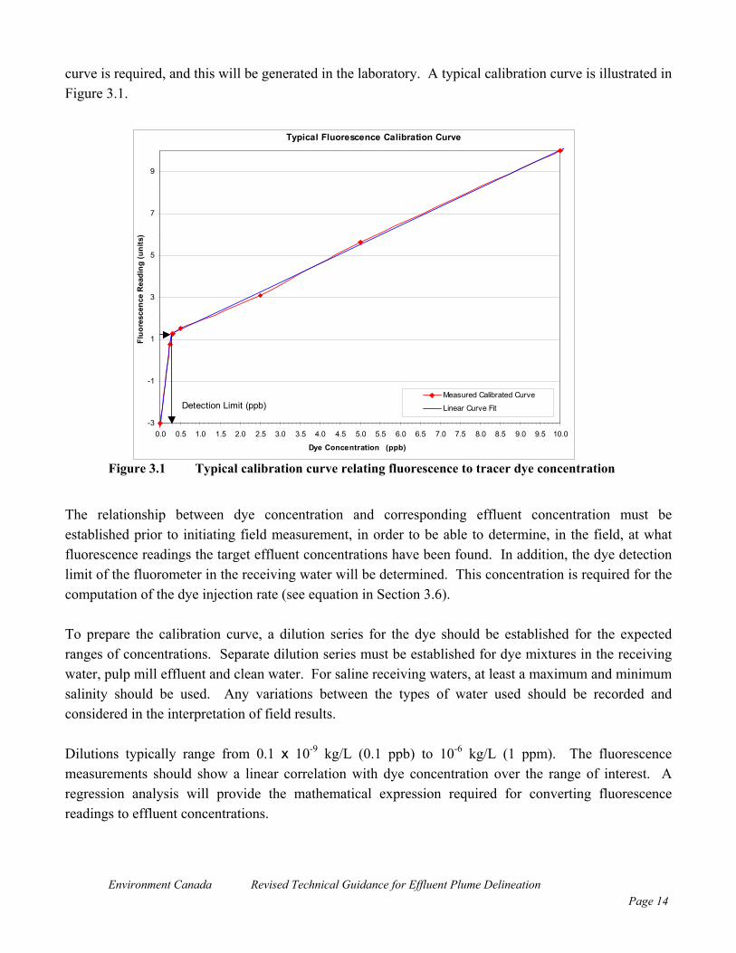
curve is required, and this will be generated in the laboratory. A typical calibration curve is illustrated inFigure 3.1.
Figure 3.1 Typical calibration curve relating fluorescence to tracer dye concentration
The relationship between dye concentration and corresponding effluent concentration must beestablished prior to initiating field measurement, in order to be able to determine, in the field, at whatfluorescence readings the target effluent concentrations have been found. In addition, the dye detectionlimit of the fluorometer in the receiving water will be determined. This concentration is required for thecomputation of the dye injection rate (see equation in Section 3.6).
To prepare the calibration curve, a dilution series for the dye should be established for the expectedranges of concentrations. Separate dilution series must be established for dye mixtures in the receivingwater, pulp mill effluent and clean water. For saline receiving waters, at least a maximum and minimumsalinity should be used. Any variations between the types of water used should be recorded andconsidered in the interpretation of field results.
Dilutions typically range from 0.1 x 10⁻⁹ kg/L (0.1 ppb) to 10-6 kg/L (1 ppm). The fluorescencemeasurements should show a linear correlation with dye concentration over the range of interest. Aregression analysis will provide the mathematical expression required for converting fluorescencereadings to effluent concentrations.
Typical Fluorescence Calibration Curve
-3
-1
1
3
5
7
9
0.0 0.5 1.0 1.5 2.0 2.5 3.0 3.5 4.0 4.5 5.0 5.5 6.0 6.5 7.0 7.5 8.0 8.5 9.0 9.5 10.0
Dye Concentration (ppb)
Fluo
resc
ence
Rea
ding
(uni
ts)
Measured Calibrated Curve
Linear Curve FitDetection Limit (ppb)
Environment Canada Revised Technical Guidance for Effluent Plume DelineationPage 15
3.8 Equipment Used to Track Currents and Effluent Movement
Drogues and current meters are the basic types of equipment that may be used to track the movement ofcurrents and thereby also the movement of an effluent. A description of each type is provided below.
3.8.1 Drogues
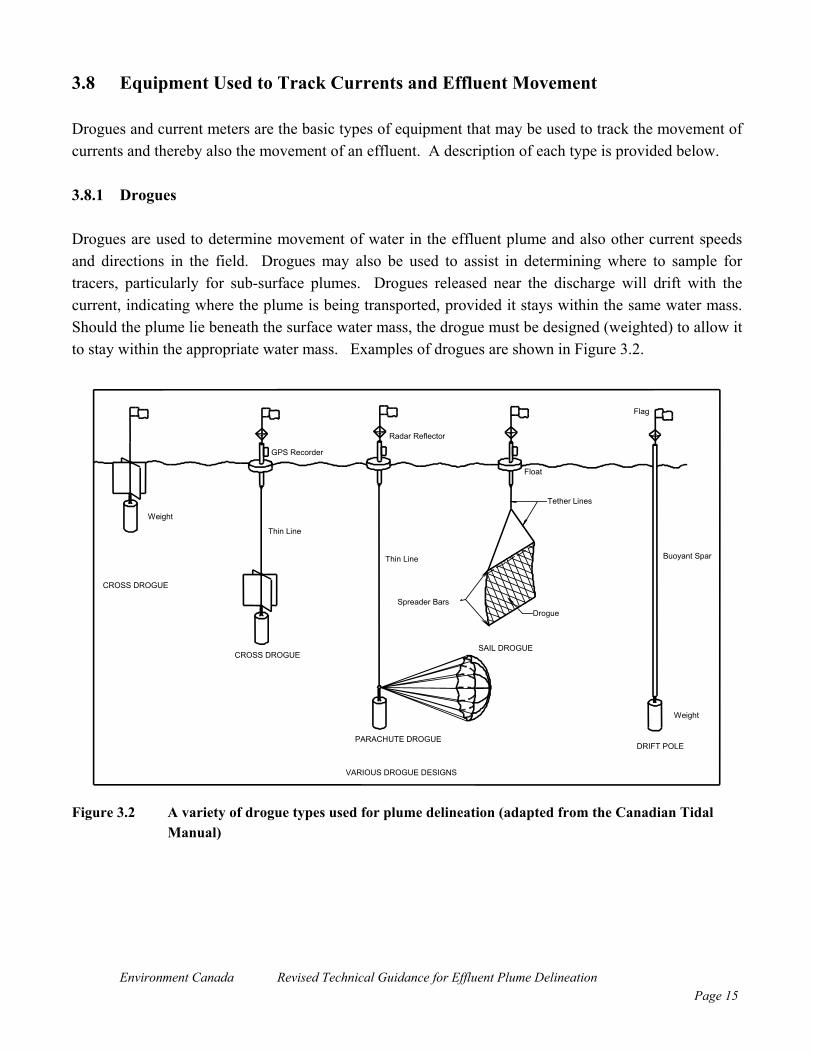
Drogues are used to determine movement of water in the effluent plume and also other current speedsand directions in the field. Drogues may also be used to assist in determining where to sample fortracers, particularly for sub-surface plumes. Drogues released near the discharge will drift with thecurrent, indicating where the plume is being transported, provided it stays within the same water mass.Should the plume lie beneath the surface water mass, the drogue must be designed (weighted) to allow itto stay within the appropriate water mass. Examples of drogues are shown in Figure 3.2.
Weight
PARACHUTE DROGUE
Flag
Radar Reflector
Thin Line Buoyant Spar
Float
Tether Lines
DrogueSpreader Bars
SAIL DROGUE
Thin Line
GPS Recorder
CROSS DROGUE
CROSS DROGUE
VARIOUS DROGUE DESIGNS
DRIFT POLE
Weight
Figure 3.2 A variety of drogue types used for plume delineation (adapted from the Canadian TidalManual)
Environment Canada Revised Technical Guidance for Effluent Plume DelineationPage 16
Drogues that are used to follow surface waters should be a relatively simple design, such as the “crossdrogue” (Figure 3.2) made of two sheets of plywood weighted to keep the upper edge of plywood justbelow the water surface (50 cm or less). The dimensions of each vane should be not less than about 30cm but otherwise can be constructed to a scale appropriate to conditions. Visual location of the drogueis typically marked by a flagged rod sticking out of the water and/or by a surface float, although acousticmarkers may also be used (see below). The use of a surface float with some reserve buoyancy makessure the drogue always remains at the correct depth in the water column. It is important that the windresistance of any marker or the drag of the surface float will be minimal compared to that of the drogueitself. If there is considerable wave action or turbulence, then the distance between the surface float anddrogue should be increased (see “cross drogue” with longer shaft in Figure 3.2) to ensure that the upperedge of the drogue does not flip out of the water and become influenced by wind forces. To check thatthe drogue is remaining within the same water mass as the plume, measurement of a simple parameter(e.g., temperature, salinity) alongside the drogue may be used.
Some drogues should be placed in the water to determine surface water movement and a few should beplaced at greater depth, particularly if the plume may plunge or be entrapped at a lower layer. Thedrogue tracks will give visual confirmation of the likely plume track. In estuarine and marineconditions, the drogues need to be dropped in the discharge area at high water, low water and both midtides. Since it is desirable that some of the earlier drogues are allowed to run the full course, asignificant number of drogues may be required. On board plots on charts can be used to track droguemovement, which should greatly assist in recovery of the drogues.
There may be situations in which the plume may remain below the surface or may plunge later. In bothcases, the plume will be moving below a less dense water mass at the surface. Some guidance can stillbe obtained in these cases using the same basic drogue design but taking care to weight the drogue sothat it represents the same density as the displaced water of the plume. A long, slack line to the surfacebuoy of the drogue will enable the drogue location to be approximated. Alternatively, an acousticlocator can be attached to the drogue. These “acoustic drogues” are used to track movement ofsubmerged plumes in the open ocean and may also be used in shallower water to estimate drift (belowthe threshold of most current meters) of the lower layers in a fjord or a large lake. Depending on themixing in the plume this will suffice only for a few kilometres because the density in the plume will beconstantly changing as it mixes with lighter surface and denser deeper water on its upper and lowerboundaries. These types of plume behaviour are discussed in more detail in Section 5.
3.8.2 Current Meters
Current meters may be used to describe the hydrodynamics of receiving waters, and in particular thespatial variability in currents for use in a numerical model. Most current meters can record temperatureand salinity as well, providing additional information about the types of water masses that are moving.However, current meters are typically more expensive to use than drogues in plume delineation studies.
Environment Canada Revised Technical Guidance for Effluent Plume DelineationPage 17
Current meters are particularly useful for large lakes and marine waters where currents are rotary, orwhere wind and wave action may be the dominant current inducer. In these environments, currentmeters may be deployed at near-surface and mid-depth during selected seasons of the year (minimum 30day deployment) to describe the currents. A good description of modern current meters is given in IEEE(2003).
The Acoustic Doppler current meter is a more sophisticated type of current meter that is versatile andhas been used in EEM studies. There are limitations for use of this meter type for plume delineation,including the following: it is expensive; interpretation of the results requires an experiencedhydrographer; poor resolution of data obtained close to the water-air and water-bottom substrateinterfaces when using the full depth range (this is a problem when tracking buoyant plumes that tend tobe initially in the upper meter of water).
3.9 Tracking Effluent Dispersion
Standard guidance is provided in this section for tracking effluent in a simple unidirectional flowreceiving environment, using Rhodamine WT as a tracer. Additional guidance is provided in Section 5for specific types of receiving environments: rivers, small lakes and impoundments, large lakes,estuaries and fjords and coastal marine. Use of an alternative tracer will require appropriatemodifications to the recommended procedure. Details on the use of Rhodamine WT are available fromfluorometer manufacturers and the U.S. Geological Survey (1996).
For a mill with multiple discharges, each discharge should be traced separately at different times todetermine the configuration of each effluent plume. In most cases, the cumulative plume may beevaluated using numerical models. However, most of the mills in Canada have consolidated theireffluent discharges so that only one point of discharge is typically relevant.
3.9.1 Sampling in the Initial Dilution Zone
Sampling in the rising plume is difficult and unproductive for the purpose of plume delineation. Instead,sampling should be focused in the area where the plume breaks the surface or is arrested in its verticalascent. This point may be several tens of meters down drift of the discharge point. Concentrations ordilutions may vary as much as 50% around the point of emergence. Sampling should be undertaken toconfirm the variability of effluent concentration at right angles to the flow of the receiving water andalso parallel to the flow.
Additional sampling should be undertaken at right angles to the flow approximately 50 to 100 m down-flow from the surface plume break-out to determine the plume width, thickness and depth. From this
Environment Canada Revised Technical Guidance for Effluent Plume DelineationPage 18
point on, further mixing would be considered to be beyond the initial dilution zone and sampling shouldbe as recommended below.
3.9.2 Subsequent Dispersion
Beyond the initial dilution zone, the effluent plume typically moves horizontally, borne by the velocityof the receiving waters. At this point, drogues released within the surface plume will provide guidanceon plume location. The following description of subsequent dispersion refers to surface plumes; specificguidance for plunging or trapped plumes is provided in Section 5.4.
Sampling traverses should be conducted at right angles to the flow of the plume and at intervals ofapproximately 5 times the last plume width. The fluorometer or hose intake should be held at a constantdepth while the boat traverses the plume. The recommended sampling depth is 1 m in homogeneouswater, possibly less in stratified flow, and possibly deeper in homogeneous water if it has beendetermined that the plume is well mixed with depth. The depth of maximum tracer concentration is usedfor profiling the tracer concentration.
It is particularly important to locate both edges of the plume and to determine if the edge of the plumetouches a shoreline. In the first few traverses, the boat should return to the center of the plume and thefluorometer or hose intake should be lowered to determine the vertical extent of the plume, and thisshould be compared with the expectation from the conceptualization of dispersion. If necessary, theboat should then return along the traverse with the fluorometer of hose intake at a deeper depth (e.g., 2to 3m) to better delineate the lower surface concentrations.
Sampling should continue until the 1:1000 dilution (i.e., 0.1% effluent concentration) limit isdetermined. It should be recognized that at the far edges of the plume, sections of the plume maybecome separated from the main plume and form independent patches of effluent that float with thecurrent.
Under no circumstances should a flow-through fluorometer be placed within 2 m of the bottomsubstrate, as this may result in equipment damage or failure. If it is suspected that the effluent plume isin or near contact with the bottom substrate, then bottled samples should be collected for subsequentanalysis (see paragraph below on “grab” samples). To confirm that this is the case, at least five samplesper cross section should be taken.
Any unusual characteristics in terms of plume location or concentration should be noted. Examplescould include high concentrations observed at places beyond where the effluent concentration hasdropped below the specified concentration (e.g., accumulation in an inlet or bay), or where an undertowmoves effluent downstream or off-shore such that effluent resurfaces elsewhere.
Environment Canada Revised Technical Guidance for Effluent Plume DelineationPage 19
Bathymetry should be measured and recorded at tracer profiling locations. Sonar techniques aregenerally adequate. Where a detailed hydrographic chart is already available, a survey of bathymetrymay not be necessary. It is recommended that bathymetric data for the receiving water be presented ona map of the exposure area.
Measurements of fresh water flow and tidal water level changes should be recorded for at least 24 hoursprior to and during the tracer release. At a minimum, these measurements should be taken hourly, butcontinuous recording is recommended.
Grab samples are recommended only if the plume is not directly accessible by the fluorometer or hoseintake. The grab sampling procedure is slower, has poor spatial resolution, and does not provide acontinuous profile of the tracer concentrations. Consequently, it is difficult to carry out a mass balanceof the tracer. Nevertheless, it is sometimes necessary to collect grab samples. Grab samples should becollected using a water pump or by lowering sample bottles that are under vacuum pressure. Use of aNiskin or similar sample collection bottle for multiple-use is not recommended because of the risk ofcontamination from previous sampling. Grab samples should be stored in the dark under refrigeration,and be analyzed within 24 to 48 hours. If samples are to be collected only by this method, then at least12 samples at each transect are recommended from within the plume to adequately define the plumeconfiguration. It is expected that at least 10 cross sections would be sampled for any of the plumesresulting from a discharge.
3.10 Data Quality
Using the site-specific calibration curve (Figure 3.1), fluorescence readings are converted from unit-lessvalues to dye concentrations in µg/L (i.e., ppb), and then to percent effluent. A similar unit conversionis necessary for naturally occurring tracers. Compensation for temperature changes and varying effluentdischarge quantities during the field test may be required. The results should be displayed in tabularformat listing time (for marine conditions, use time relative to high or low tide), water level, position,salinity (if applicable), immersion depth of the sonde or sampling tube, local water depth (optional), dyeconcentration and calculated effluent concentration.
A discussion on the confidence limits of the results should consider the effects of such factors asenvironmental conditions during the test, method of testing to measure fluoresence (e.g., grab samples,pump-through, immersed fluorometer), accuracy of the positioning data, variation in effluent discharge,and confidence in the calibration curve.

Environment Canada Revised Technical Guidance for Effluent Plume DelineationPage 20
3.11 Numerical Modeling
Numerical modeling provides a means of extrapolating from the plume measurements in the field tosimulate effluent dispersion over a much wider range of environmental conditions at the site. Numericalmodels have been developed that superimpose water quality computations onto hydrodynamicprocesses. The models allow for a qualitative and graphic representation of the transport and dispersionof the effluent (tracer) in time and space.
Depending on the nature of the receiving water, two or three-dimensional models may be used.Principal processes in numerical modeling include model setup, model calibration and verification (bothof which use the field tracer study results), and a sensitivity analysis to determine what limitations mayhave to be placed on input parameters. While model calibration should be carried out against the mostrecent tracer measurements, verification can be achieved by applying the model to an historical eventwith different environmental and discharge conditions. After successful calibration, verification andsensitivity analysis, the model is then ready to be applied to a number of environmental conditions thatmay lead to effluent plume dispersions other than the dispersion observed during the fieldmeasurements. A discussion should be provided on the frequency of the various environmentalconditions being considered.
As a minimum, the models used should be able to accurately reproduce the hydrodynamic process of thestudy area and the behaviour of a conservative substance introduced near the discharge. The initial nearfield dilution may be computed using descriptive models, such as Cormix or Visual Plumes. The tracerconcentrations computed for the edge of the near field can then be used as boundary conditions for thefar field model. Other typical boundary conditions for far field models are the fresh water input on theupstream end and the water level on the downstream end. In river systems with fast flowing currents,the models have to be able to simulate sub and supercritical flow conditions. In tidal waters, where theshore line near the discharge changes from high to low tide, the model should be able to reproducewetting and drying of tidal flats.
The near field and two-dimensional far field models are readily available and have been commonly usedfor effluent plume delineations of pulp mill effluents. The three-dimensional models are very costly topurchase and require a significant effort for data collection, model setup and calibration. Somehydrographic research institutes are well equipped for applying three-dimensional models.
Table 3.2 lists potentially applicable models for a variety of effluent discharge scenarios, and includesmodels that are commercially available and routinely used. This table is intended as a preliminary guideonly because models are constantly being developed and modified, and because there are many modelsnot listed that are developed for in-house use only, and are therefore not commercially available.

Environment Canada Revised Technical Guidance for Effluent Plume DelineationPage 21
Table 3.2 Numerical Models for Describing Effluent Dispersion
Typical Scenario Information Needs for EEM Examples of Commercially AvailableNumerical Models 1
Plume is highly transitory or thereis rapid plume dilution in the initialdilution zone to within target level(i.e., 1% effluent concentration)
Conceptual spatial delineation of1% and 0.1% limits of effluentconcentration. Whether the 1% concentrationlimit is reached within 250 m fromthe discharge.
Numerical models such as Cormix and VisualPlumes for the initial dilution assessment only
Effluent is discharged intoturbulent, narrow stream; completemixing is achieved rapidly over ashort distance
Linear distance until plume isdissipated to within target levels(i.e., 0.1% and 1% effluentconcentration)
1D numerical models, such as HEC-5Q, Qual1E , WASP5/Dynhyd5
Effluent is discharged intouniform, wide body of water. Nostratification is observed.
Length and width distance untilplume as dissipated to target levels(i.e., 0.1% and 1% effluentconcentration)
Numerical models such as Cormix for initialplume dilution, 2D numerical models, such asRMA 2/RMA 4, Qual 2E, MIKE 21, forsubsequent dilution simulations
Effluent is discharged into non-uniform, wide body of water.Stratification is observed as resultof thermal or salinity differences inthe receiving water or between theeffluent and the receiving water.Stratification may be non-uniformand dynamic.
Length, widths and depth dilutionsuntil plume as dissipated to targetlevels (i.e., 0.1% and 1% effluentconcentration)
Numerical models such as Cormix and VisualPlumes for initial dilution assessments, only.3D numerical models, such as RMA10/RMA11, WASP5/Dynhyd5, MIKE 3,TELEMAC, DELFT 3D for far fieldsimulations.
1 Sources for these models vary; some may be obtained directly from the model developers while others may beobtained from one or a number of commercial distributors.
The selected numerical model should be used to estimate the desired regions of maximum extent,average conditions, and minimum dilution. A discussion on the confidence limits of the results shouldbe provided (see Section 3.10).
If current meters are being used to measure ambient currents (see Section 3.8.2), the modeled plumeconfiguration may be modified through statistical analysis of the current meter data. For conditions of along flushing period, the measured dye concentrations may be used to calibrate a numerical transport-diffusion model. The model can then be used to simulate the effluent delineation and characteristicsarising from a continuous discharge. The model can be run for a variety of conditions (e.g., seasonalvariations of water movements and wind patterns), thereby overcoming the limitations of the particularconditions recorded in a single field study.
Additional resources for guidance on numerical modeling include: Baumgartner et al. (1994), Chungand Roberts (1998), Ettema et al. (2000), Frick et al. (2000), and Sharp (1989).
Environment Canada Revised Technical Guidance for Effluent Plume DelineationPage 22
4.0 REPORTING
Reporting of the study results should include the following:
1. Summary of information collected to aid in developing the conceptual model of effluent plumebehaviour, including:• description of the effluent in terms of flow, temperature, specific gravity and TSS (if applicable);• description of the effluent discharge configuration and performance;• description of the receiving environment in terms of flows and currents, physical and chemical
water quality (e.g., thermal and salinity variation horizontally and vertically), climaticconditions, and any other relevant site-specific parameters used to develop the conceptual modelof plume behaviour; and
• confounding conditions, such as pulp and paper mill upsets, atypical climatic conditions.
2. A conceptualized model of plume behaviour.
3. Documentation of tracer study conducted, including:• pre-tracer laboratory testing, fluorometer calibration curve;• pre-trial field testing; and• trial field tracer measurements.
4. The Numerical model used and mapping depicting predicted plume envelopes for:• maximum extent (1% and 0.1% effluent concentrations); and• long-term average conditions (1% and 0.1% effluent concentrations).
Computer animation is a useful option for depicting effluent plume behaviour in more complexreceiving environments, such as estuaries and coastal locations.
The measured tracer concentrations should be provided in the appendix of the report.
Environment Canada Revised Technical Guidance for Effluent Plume DelineationPage 23
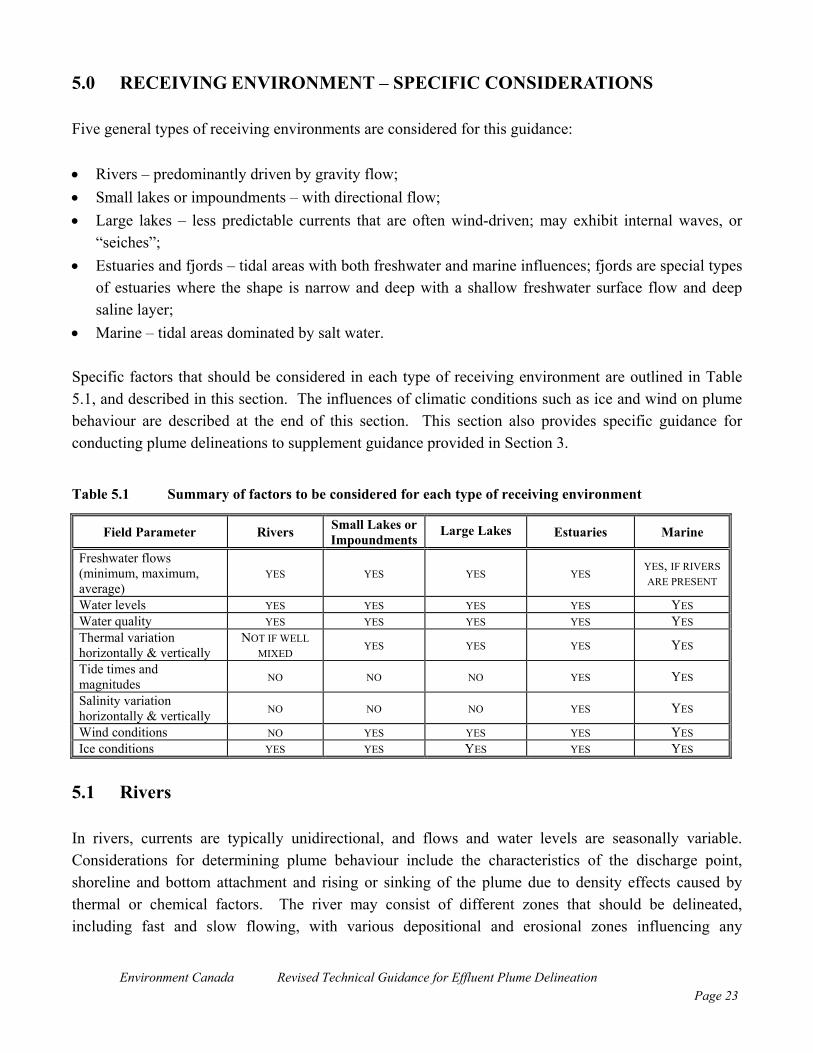
5.0 RECEIVING ENVIRONMENT – SPECIFIC CONSIDERATIONS
Five general types of receiving environments are considered for this guidance:
• Rivers – predominantly driven by gravity flow;• Small lakes or impoundments – with directional flow;• Large lakes – less predictable currents that are often wind-driven; may exhibit internal waves, or
“seiches”;• Estuaries and fjords – tidal areas with both freshwater and marine influences; fjords are special types
of estuaries where the shape is narrow and deep with a shallow freshwater surface flow and deepsaline layer;
• Marine – tidal areas dominated by salt water.
Specific factors that should be considered in each type of receiving environment are outlined in Table5.1, and described in this section. The influences of climatic conditions such as ice and wind on plumebehaviour are described at the end of this section. This section also provides specific guidance forconducting plume delineations to supplement guidance provided in Section 3.
Table 5.1 Summary of factors to be considered for each type of receiving environment
Field Parameter Rivers Small Lakes orImpoundments
Large Lakes Estuaries Marine
Freshwater flows(minimum, maximum,average)
YES YES YES YESYES, IF RIVERSARE PRESENT
Water levels YES YES YES YES YESWater quality YES YES YES YES YESThermal variationhorizontally & vertically
NOT IF WELLMIXED
YES YES YES YES
Tide times andmagnitudes NO NO NO YES YES
Salinity variationhorizontally & vertically NO NO NO YES YES
Wind conditions NO YES YES YES YESIce conditions YES YES YES YES YES
5.1 Rivers
In rivers, currents are typically unidirectional, and flows and water levels are seasonally variable.Considerations for determining plume behaviour include the characteristics of the discharge point,shoreline and bottom attachment and rising or sinking of the plume due to density effects caused bythermal or chemical factors. The river may consist of different zones that should be delineated,including fast and slow flowing, with various depositional and erosional zones influencing any
Environment Canada Revised Technical Guidance for Effluent Plume DelineationPage 24
suspended solids transport from the effluent. A discussion on the temporal changes (seasonal and longterm) of the river regime on the reaches affected by the plume should be provided.
Plume delineation studies should be conducted during a period that approaches the annual low riverflow, which typically occurs in late summer. This will leave the extreme high and medium flows to bepredicted using numerical models. Low river flows typically correspond with low overall dilutionpotential and reduced rates of turbulent mixing in the system. As a result, spatial extent of plumes tendsto be larger during periods of low flow.
If a dye tracer is used, it should be added using a continuous flow rate injection system. The number offield tracer measurements to take will be site-specific. It is recommended that concentrations bemeasured at various distances downstream and that the spatial extent of the plume be determined. Slugtests (i.e., batch release of dye, as opposed to continuous flow rate tracer injection) may be a also asuitable technique for monitoring mixing in some rivers, but this generally requires a very goodunderstanding of the plume behaviour and may require repeated slugs.
5.2 Small Lakes and Impoundments
Guidance for rivers (above) will apply if there are large effluent volume discharges, because there willtypically be an easily discernable and measurable flow through the system. However, this guidance willnot apply to some small lakes and impoundments where there are residual currents, or where the long-term drift is masked or even reversed by short term effects induced by factors such as wind shear, lakeoverturning, development of thermocline, or freshets, separately or in combination. It is important toassess the magnitude and significance of each of these comparatively short-term phenomena. This ismost easily done using numerical modeling, provided there are adequate field data available for modelcalibration.
The residual flow, or even transitory currents, may be below the threshold of regular recording currentmeters. In these cases, a mass balance of the flows entering the body of water and the flows leaving willprovide an estimate of the retention time in the system. This retention time may be reduced further byassessment of special circumstances or geometry. However, where currents are very low (e.g., a fewcm/min), only field tracer studies can provide the confidence that an effluent will be carried away andthat re-circulation does not take place. Re-circulation takes place where eddies from the plume arebrought back to the mixing system and used instead of clean new receiving water. After some time thismay significantly reduce the dilution of the effluent and significantly extend the 1% concentrationboundary.
The residual flow through the area should be estimated as well as the currents that are induced by windat various strengths and from various directions. An onshore wind will typically trap water against the
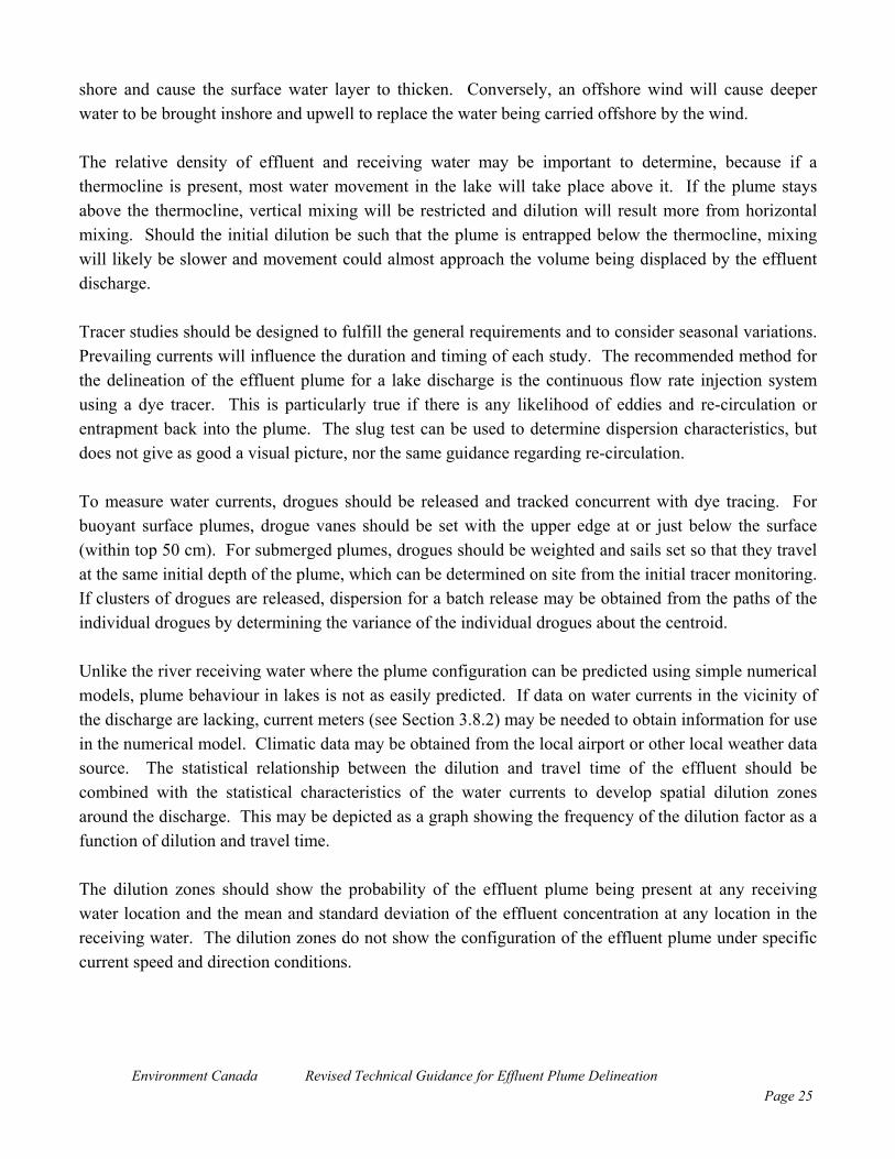
Environment Canada Revised Technical Guidance for Effluent Plume DelineationPage 25
shore and cause the surface water layer to thicken. Conversely, an offshore wind will cause deeperwater to be brought inshore and upwell to replace the water being carried offshore by the wind.
The relative density of effluent and receiving water may be important to determine, because if athermocline is present, most water movement in the lake will take place above it. If the plume staysabove the thermocline, vertical mixing will be restricted and dilution will result more from horizontalmixing. Should the initial dilution be such that the plume is entrapped below the thermocline, mixingwill likely be slower and movement could almost approach the volume being displaced by the effluentdischarge.
Tracer studies should be designed to fulfill the general requirements and to consider seasonal variations.Prevailing currents will influence the duration and timing of each study. The recommended method forthe delineation of the effluent plume for a lake discharge is the continuous flow rate injection systemusing a dye tracer. This is particularly true if there is any likelihood of eddies and re-circulation orentrapment back into the plume. The slug test can be used to determine dispersion characteristics, butdoes not give as good a visual picture, nor the same guidance regarding re-circulation.
To measure water currents, drogues should be released and tracked concurrent with dye tracing. Forbuoyant surface plumes, drogue vanes should be set with the upper edge at or just below the surface(within top 50 cm). For submerged plumes, drogues should be weighted and sails set so that they travelat the same initial depth of the plume, which can be determined on site from the initial tracer monitoring.If clusters of drogues are released, dispersion for a batch release may be obtained from the paths of theindividual drogues by determining the variance of the individual drogues about the centroid.
Unlike the river receiving water where the plume configuration can be predicted using simple numericalmodels, plume behaviour in lakes is not as easily predicted. If data on water currents in the vicinity ofthe discharge are lacking, current meters (see Section 3.8.2) may be needed to obtain information for usein the numerical model. Climatic data may be obtained from the local airport or other local weather datasource. The statistical relationship between the dilution and travel time of the effluent should becombined with the statistical characteristics of the water currents to develop spatial dilution zonesaround the discharge. This may be depicted as a graph showing the frequency of the dilution factor as afunction of dilution and travel time.
The dilution zones should show the probability of the effluent plume being present at any receivingwater location and the mean and standard deviation of the effluent concentration at any location in thereceiving water. The dilution zones do not show the configuration of the effluent plume under specificcurrent speed and direction conditions.
Environment Canada Revised Technical Guidance for Effluent Plume DelineationPage 26
5.3 Large Lakes
Water currents in large lakes are often wind driven, seasonally variable, and generally less predictablethat those encountered in fluvial and tidal areas. Thermal and density stratification is important tounderstand because the effluent may be more dense than lake water due to chemical factors, or lessdense than lake water due to thermal factors. Wind and wave advection, seiches, shore-line and bottomattachment are all important. Many of the factors considered for small lakes and impoundments are alsorelevant to large lakes.
In large lakes, it is useful to have information on the variability in long-term water movement and theresulting residual movement. This information may be obtained using moored current meters with a lowcurrent threshold. Temperature recorders on the current meters may be used to determine whetherinternal waves or seiches occur. On shore anemometers may be used to obtain concurrent wind data ifwind data are otherwise unavailable.
Initial dispersion of the surface plume into a relatively quiescent lake will be significantly influenced bythe volume of the upwelling plume. Numerical modeling is the strongest tool to delineate the plume tothis stage. Subsequent dispersion using numerical modeling will require estimates of horizontal andvertical dispersion coefficients, as well information about water currents obtained from current meters.The dispersion coefficients are best determined by either a slug release of dye or by continuous releaseand subsequent monitoring of a tracer in the effluent plume. If wind is present, an estimate of inducedwind drift current can be determined using wind drift forecasting curves (see Section 5.6.2). Winds canalso induce tilting of the water surface and of the thermocline, which may result in seiche motions thatoscillate within the basin. See Section 5.6.2 for more discussion on wind-induced seiches.
Two-dimensional numerical modeling may be adequate, however in situations where there isstratification, three-dimensional modeling may be necessary.
5.4 Estuaries and Fjords
Estuaries and fjords are complicated environments in which to conduct plume studies. Anunderstanding of the nature of the receiving waters is very important for planning the field study. Thissection will first provide a description of hydrographic considerations in estuaries and fjords, followedby guidance for conducting field studies.
5.4.1 Hydrographic Considerations
The most significant influences on effluent dispersion in estuaries and fjords are tidal flows and densitydifferences between freshwater and saltwater. Tides cause water to flow into an estuary on the rising
Environment Canada Revised Technical Guidance for Effluent Plume DelineationPage 27
tide and flow out again during the falling tide, causing mixing to take place. Effluents are typicallysimilar in density to fresh water and will therefore tend to follow the fresh water in their mixing pattern.Freshwater has a specific gravity of about 1.00. Effluent and freshwater will typically rise and flowalong the top of saltwater, which has a specific gravity of about 1.026.
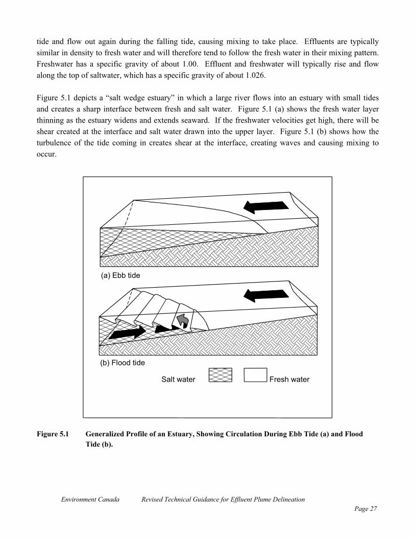
Figure 5.1 depicts a “salt wedge estuary” in which a large river flows into an estuary with small tidesand creates a sharp interface between fresh and salt water. Figure 5.1 (a) shows the fresh water layerthinning as the estuary widens and extends seaward. If the freshwater velocities get high, there will beshear created at the interface and salt water drawn into the upper layer. Figure 5.1 (b) shows how theturbulence of the tide coming in creates shear at the interface, creating waves and causing mixing tooccur.
Salt water Fresh water
(a) Ebb tide
(b) Flood tide
Figure 5.1 Generalized Profile of an Estuary, Showing Circulation During Ebb Tide (a) and FloodTide (b).
Environment Canada Revised Technical Guidance for Effluent Plume DelineationPage 28
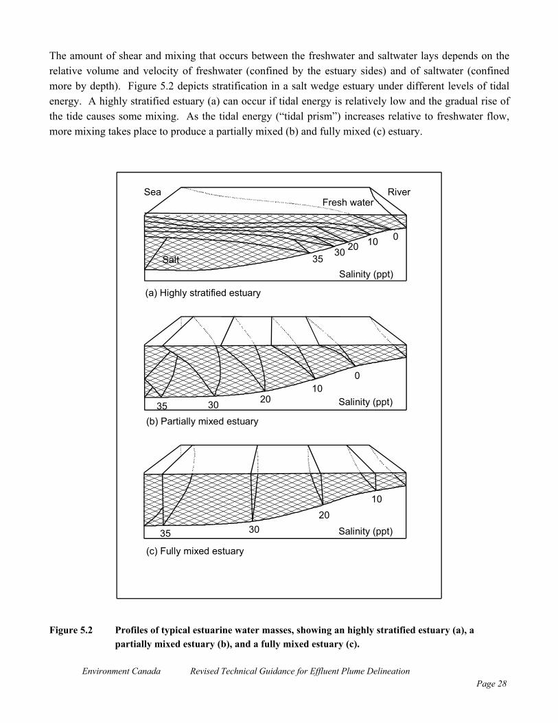
The amount of shear and mixing that occurs between the freshwater and saltwater lays depends on therelative volume and velocity of freshwater (confined by the estuary sides) and of saltwater (confinedmore by depth). Figure 5.2 depicts stratification in a salt wedge estuary under different levels of tidalenergy. A highly stratified estuary (a) can occur if tidal energy is relatively low and the gradual rise ofthe tide causes some mixing. As the tidal energy (“tidal prism”) increases relative to freshwater flow,more mixing takes place to produce a partially mixed (b) and fully mixed (c) estuary.
SeaFresh water
River
Salt
010203035
35 30 2010
0
35 3020
10
Salinity (ppt)
Salinity (ppt)
Salinity (ppt)
(a) Highly stratified estuary
(b) Partially mixed estuary
(c) Fully mixed estuary
Figure 5.2 Profiles of typical estuarine water masses, showing an highly stratified estuary (a), apartially mixed estuary (b), and a fully mixed estuary (c).
Environment Canada Revised Technical Guidance for Effluent Plume DelineationPage 29
Tidal frequency and magnitude are considered when planning a plume delineation study and insubsequent numerical modeling. Tides in Canadian estuaries typically rise and fall with approximately12.42 hours between high waters. The vertical range between high and low water, even within onecoastal system, can range is from a few centimetres to several metres. Also, there is a beat every 7, 14and 29 days indicating the “spring and neap” cycles where the forces of the sun and moon first acttogether and then oppose. In some areas of Canada every second high or low water differs considerablyfrom its predecessor. These differences are generally referred to as semidiurnal and diurnal responses ofthe particular water mass to the differing pulls of sun and moon.
Other considerations for conducting plume delineation studies in estuaries include the following:
• duration of the tidal cycle: it is not uncommon for the duration of the falling tide to exceed 7 hoursand the time of the rising tide to be significantly less than 6 hours; and
• slack tide: in some estuaries, a slack period can occur in vertical and horizontal movement aroundhigh and low water; this can amount to a few minutes or in exceptional cases almost an hour (in thiscase generally low water only); lack of significant horizontal movement for a period can lead toconsiderable pooling of effluent in the area of the discharge, leading to possible expansion of theboundary of the zone of >10% effluent concentration.
A special case occurs in fjords where the depth of the estuary is well over ten times the thickness of thetidal prism. Here the longitudinal profile will look like a salt wedge estuary or a well-stratified estuarywith the fresh water lying in a layer at the surface and very significant water depth below. The tide canrise and fall, causing negligible mixing, except possibly at the entrance where there is typically a sharpsill. In some fiords there may be a 2 to 10 m thick layer of fresh water that extends the full length of theestuary with an interface of less than a meter thick. In longer fjords extending over several tens ofkilometres, diffusion and other influences such as wind and internal waves will cause this interfaciallayer to thicken and the upper layer to become brackish.
Estuaries may demonstrate two or more estuarine types along their length or during seasonal variation inriver flow or in the spring to neap tidal cycle. In partially mixed estuaries or well stratified estuaries,there is often little seaward movement along the bed during the ebbing tide creating an increase instratification during this period. On the flood tide, the stronger currents run deep and conditions closerto well mixed are more likely to occur. In Canada, because of the Coriolis force and the difference indensity between salt and fresh water, ebb currents tend to run stronger and salinity tends to be lowertowards the right hand bank (looking seaward) of an estuary when looking seaward. Similarly, floodtide currents are stronger and salinities higher towards the left when looking seaward. This can be verymarked in wide estuaries. Where an estuary has a high fresh water discharge or a narrow exit to theopen coastal waters, a fresh or brackish water plume can extend well out to sea particularly during the
Environment Canada Revised Technical Guidance for Effluent Plume DelineationPage 30
ebb tide. Depending on the dynamics at such an entrance a portion of this plume may re-enter theestuary with the flood tide.
An estuary can change from one stratification type to another, either with distance or with time. Duringspring run-off, freshwater may dominate the upper reaches of the estuary and create a higher degree ofstratification downstream. During lower flow periods, the upper reaches of the estuary will return topartially mixed conditions and the lower salinity water will penetrate much further upstream. Internalwaves (or seiches) may form along the fresh or brackish water/salt water boundary in fjords andestuaries as a result of wind action, and may temporarily affect plume dispersion. These seiches arediscussed in more detail in Section 5.6.2.
During slack tide, a significant pool of effluent can gather in the vicinity of the discharge pipe and at aconcentration close to that delivered at the top of the rising plume. Once the horizontal tidal currentsbegin to move again, this large effluent pool is the leading edge of the effluent plume and may takesome time to dissipate. As the tidal currents strengthen, the effluent leaving the discharge area willbehave more like a standard streaming pool. If the effluent pool gathered during the low water slack, therising tide will typically come underneath the plume as denser water and carry the effluent poolupstream. The somewhat diluted effluent in the pool may pass down through the discharge area on thefalling tide and provide already polluted water to the discharging effluent. If the effluent pool gatheredduring the high water slack, it will tend to stream off downstream in a very thin layer due to densitydifferences. When the tidal currents strengthen, this high water pool of effluent will tend to dispersemore quickly than the low water effluent pool, but it may substantially extend the limit of the plume atthe surface, particularly if it is shore-attached.
Plunging plumes may occur in estuaries and fjords. Effluents with a fairly high initial dilution on therising jet can pick up salinity from the lower layers such that the plume attains a density greater than thatof the surface layer. If the rising momentum is sufficient, the plume may break the surface and thenslowly plunge or sink down to a water layer consistent with its density and travel and mix with thislower layer. This is depicted in Figure 2.1 (i).
In other situations, particularly where the surface layer is thick or very distinct, the jet will rise but betrapped at the interface between the upper and lower layer. This is likely to be the case in fjords if theinitial discharge is located in the deep saline layer. Effluent mixing into the upper layer is more likelyduring an ebbing tide. During a rising tide, the strength of the current in a shallow estuary is close to thesea floor and may cause significant mixing with, and entrainment into, the lower layers.
Submerged plumes may resurface when the plume encounters an influx of differing density watercoming into the receiving water. In this case, surface water will initially plunge, but will resurface downdrift. This scenario may occur if there is an influx of less dense water downstream of the discharge,such as from a tributary or another major effluent discharge.
Environment Canada Revised Technical Guidance for Effluent Plume DelineationPage 31
5.4.2 Conducting the Field Work
Two boats are recommended for tracer studies in estuary environments. The recommended techniquefor dye tracer measurement is use of a fluorescence sensor or sampler intake off the bow of the boat, asdescribed in Section 3.3.3. Salinity and temperature verticals should be taken along the centre line ofthe estuary and in the vicinity of the discharge. The sampling time should be noted relative to time ofhigh or low water, and sampling should always proceed in a counter current direction relative to thereceiving water movement.
It is important to consider the differences between successive high waters and between spring and neaptidal ranges and reconcile them with establishing the representative density regime in the estuary andalso the objectives of the plume delineation study. The vertical range relative to the water depth at lowtide gives some indication of potential turbulence. Another method, but requiring more work, is toestimate the water volume passing various sections during flood and ebb and hence to obtain the averagevelocities. This is particularly valuable where there are large inter-tidal volumes or additional riverflows added at particular points along the estuary.
If using a dye tracer, injection should begin about half an hour before the turn of the tide so that thestudy may begin around low water. For most estuary studies, the plumes can be delineated in the fieldin the same way as a river plume. When sampling, the boat should always work against the tidalcurrents to avoid just drifting with the receiving water and possibly sampling the same water mass. If aseparate boat is doing the drogue work or when being done on a separate day, it is useful to checksalinity and temperature at the drogue depth each time the position is confirmed. Care must be takenwhen the tide reverses and the partly diluted effluent comes back over the discharge point as there willprobably be a new thin poorly diluted plume on top of a thicker well mixed plume. When the differencein flood and ebb tide surface excursions is small (e.g., < 20% of the excursion) there may be a build upof effluent from more than one tide. Generally the numerical model can provide the most effectivepredictions of this phenomenon.
For plunging plumes, drogues can be set to follow the plume at depth. However, caution should betaken to ensure that the vertical dimension of vanes is not too large, because the upper and lower edgesmay get caught in two different water flows. If the depth of the plume is known from initial fieldsampling, the plume may be tracked as outlined in Section 3.9, except that instead of air there is a layerof water above the plume. This is one case where a fluorescence sensor or sampler intake may be towedastern, because it is likely to be well below the influence of mixing from the boat hull and propulsionunit. This technique requires more boat operator skill to maintain constant speed either with a waterspeed gauge or a revolution counter. A depressor will hold the fluorometer head or intake down, but adepth gauge (either pressure or upward looking sonar) is essential to record depth.
Environment Canada Revised Technical Guidance for Effluent Plume DelineationPage 32
It is much more challenging to follow a plume that rises to the surface and then plunges and also wherethere is no well marked interface. Initial field measurements of salinity taken to characterize theenvironment will demonstrate how the naturally occurring surface layer behaves relative to the lowerlayer down drift.
Numerical modeling may need to be carried out over a number of tidal cycles to show short-term andlong term effluent dilution fields. Three-dimensional modeling may be required for stratified receivingwaters.
5.5 Marine
Thermal and salinity stratification are important features to assess for coastal marine environmentsbecause the effluent is usually less dense than sea water due to chemical and thermal factors. In verycalm weather, the plume may be contained within a few centimetres of the water surface. Significantinfluences in this environment include wind and wave advection, shore-line attachment, bottomattachment, and tidal activity (often with rotary currents). Oceanic receiving waters are distinguishedfrom estuaries in that the main circulation is not dominated by fresh water in the vicinity of thedischarge. The effluent plume is diluted and transported by currents. Tidal activity, while present, doesnot always provide the main contribution to net effluent movement, but does affect effluent dispersion.A continuous dye release of one tide cycle is generally sufficient, but the duration of the numericalmodeling program may be over several tidal cycles.
The residual current patterns may be dominated by a coastal circulation pattern or by local wind andwave influences. It is useful to have local water current data, such as may be obtained from positioningcoastal current meters near the discharge. Likewise, local salinity, water temperature and wind recordsare also useful.
Prior to any dye release, the tidal heights and times at the site should be correlated to the nearestrecording tide gauge maintained by the Canadian Hydrographic Service. This is of value for the dyestudy and also in the use of current and other longer term records. Spatial salinity and temperatureprofiling should also be conducted at this time.
The initial concept of effluent dispersion should be useful for planning the dye release. Field delineationof a surface plume may follow the standard practice outlined in Section 3.9, although judgement will berequired on the spacing of the transects, particularly if the rotary current is marked and the plume beginsto come back over the discharge area. Tracking of submerged plumes should be conducted as describedin Section 5.4 above. It is usually beneficial to use larger scale drogues with radar reflectors and GPSreceivers in coastal areas, especially if wave action is present.
Environment Canada Revised Technical Guidance for Effluent Plume DelineationPage 33
From the dye tracer profiles, the effluent plume envelopes will be developed and related to the measuredcurrents, wind and waves on that day. The probability of the occurrence of these envelopes may bedetermined using statistical data from available data on water currents, and numerical models used toextend these envelopes over a broader time period to represent “average” conditions.
5.6 Climatic Conditions
Ice and wind may have significant effects on effluent dispersion. The following sections provideguidance on incorporating ice and wind conditions in interpreting plume behaviour. The applicability ofnumerical models using ice are very limited at this time.
5.6.1 Ice
Ice is a common occurrence in many Canadian water bodies during winter. Its general effect on theeffluent discharge is two-fold. Ice cover shields the receiving waters from the effects of wind stress andmay also alter or cause stratification in the water column and hence modify water circulation. However,in the case of land fast ice, the underside of the ice provides a solid rough boundary to flow and createsturbulence similar to flowing over the stream bottom.
Most effluents are warm and this will cause some melting and a weakened ice surface. The buoyantplume will cling to this ice surface in the same way that a dense plume will cling to the bottom substrate.As far as is known, no detailed effluent plume field studies have been made under ice conditions, but itis reasonable to assume that mixing is likely to be decreased. This can result in the extent of plumeconcentrations being under-estimated when based on open water considerations alone.
Land fast ice cover removes wind stress mixing from the surface waters. In the presence of fresh waterdischarges (e.g., river discharges), mixing will be reduced between the effluent and river water. Ridgesmay appear in the formation of the ice surface. Some of these ridges may be the result of early ice flowscolliding, and others may be formed by thermal expansion of the ice. Ridges may form in the sameposition each year and may have a keel or downward projection as much as 7 times the height of thesurface ridge. These ridges can interfere with the plume and may divert it in a very different direction toits normal open water mode.
Moving ice still generally shields the surface water from direct wind effects. However, wind influencesmay be greater than initially predicted, because wind motion will be transmitted from the below waterprofile of ice flows to the receiving water and/or the plume. Where moving ice comes in contact withland fast ice or an island, a significant ice ridge may form.
Environment Canada Revised Technical Guidance for Effluent Plume DelineationPage 34
The standard numerical models for plume delineation are generally not appropriate for considering iceconditions since they assume a free water surface (i.e., open channel flow). 5.6.2 Wind
Wind acting on large bodies of water induces currents and waves in direct proportion to its strength, itsduration, and fetch over the water body. Fortunately, nomographs are available to provide estimates ofcurrent speed, and wave height and period that can contribute to understanding wind effects on thedispersion of effluents. One of the most valuable sources of information is literature relating to oil spilltrajectory modeling, or ocean search and rescue. For wind currents, the James wind-drift forecastingcurves (James 1966) are probably the easiest to use to obtain a magnitude. When using the Jamescurves, the direction is usually taken as being 20 degrees to the right of the wind direction, due toCoriolis forces.
In more detailed work this can be modified to accommodate variations in duration, fetch, wind speedand water depth, among other factors. In many coastal areas it is the predominant wind directioncoupled with local underwater topography that provides the driving force for currents along the shore.The momentum built up can make these currents very persistent. Wind waves also transport water,particularly when they get into shallow water. These waves can run out of the wind field and continueto transport their energy over hundreds of miles.
The nomograms most commonly used for wave predictions are those developed by the U.S. Army Corpsof Engineers (1984). Wind wave energy is transmitted in two ways: first, on the surface by waterparticles orbiting in a circular motion with a radius of half the wave height at the surface; and second, atdepth with the radius diminishing to almost zero at a depth of half the wave length. Typical coastalwaves have periods of 4, 6, and 8 seconds, and have wave-lengths of 25 m, 56 m and 100 m,respectively. When this motion at a depth of half wave length comes in contact with the bottomsubstrate, friction causes the wave to slow and the circular particle motion changes to elliptical. On along beach, this will cause the wave crests to try to align themselves parallel to the contours andeventually the shore. This has two effects on the plume: increased mixing within the plume andcurrents along the shore generated by the waves.
Internal waves, or seiches, moving along the interfacial boundary between two water masses can alsoimpact the dispersion of a plume. The generation of these waves is not well understood but they areformed as eddies by the shear forces acting between the two opposing water layers, and they may befound moving along the thermocline in lakes, the sharp fresh water/salt water boundary in fiords, orbetween the estuarine and marine water in large estuaries or coastal waters. These internal waves can beof large amplitude (e.g., on the order of meters) with waves of 80 m being recorded in the St Lawrenceoff the Saguenay. Their impact on the plume is transitory, and are mentioned here only for guidanceshould an anomaly occur during a dye test. Their occurrence would be picked up on the records ofrecording thermographs or salinometers.
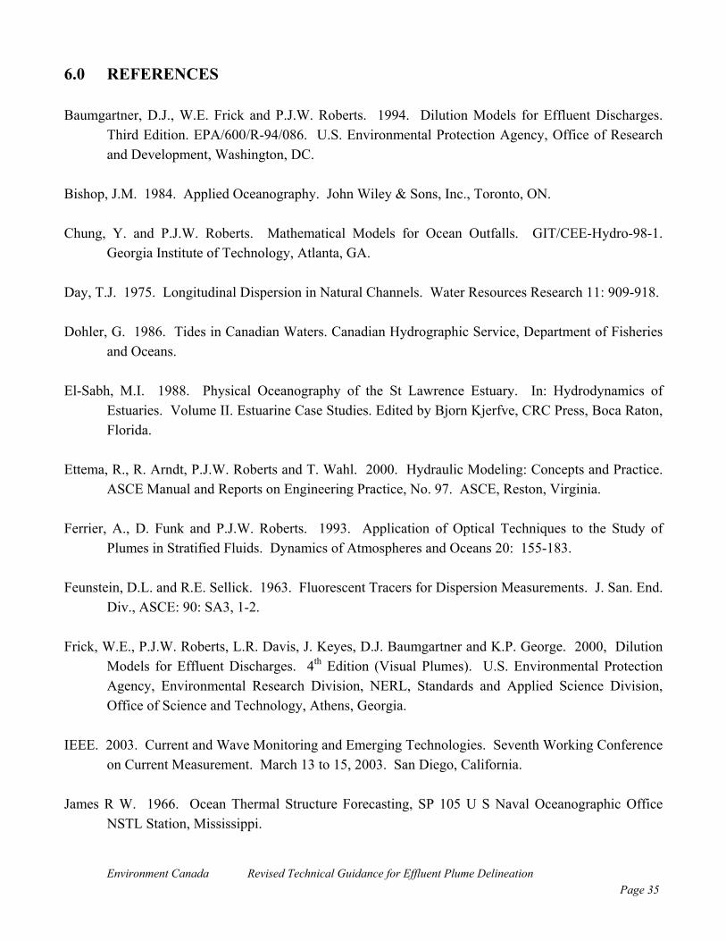
Environment Canada Revised Technical Guidance for Effluent Plume DelineationPage 35
6.0 REFERENCES
Baumgartner, D.J., W.E. Frick and P.J.W. Roberts. 1994. Dilution Models for Effluent Discharges.Third Edition. EPA/600/R-94/086. U.S. Environmental Protection Agency, Office of Researchand Development, Washington, DC.
Bishop, J.M. 1984. Applied Oceanography. John Wiley & Sons, Inc., Toronto, ON.
Chung, Y. and P.J.W. Roberts. Mathematical Models for Ocean Outfalls. GIT/CEE-Hydro-98-1.Georgia Institute of Technology, Atlanta, GA.
Day, T.J. 1975. Longitudinal Dispersion in Natural Channels. Water Resources Research 11: 909-918.
Dohler, G. 1986. Tides in Canadian Waters. Canadian Hydrographic Service, Department of Fisheriesand Oceans.
El-Sabh, M.I. 1988. Physical Oceanography of the St Lawrence Estuary. In: Hydrodynamics ofEstuaries. Volume II. Estuarine Case Studies. Edited by Bjorn Kjerfve, CRC Press, Boca Raton,Florida.
Ettema, R., R. Arndt, P.J.W. Roberts and T. Wahl. 2000. Hydraulic Modeling: Concepts and Practice.ASCE Manual and Reports on Engineering Practice, No. 97. ASCE, Reston, Virginia.
Ferrier, A., D. Funk and P.J.W. Roberts. 1993. Application of Optical Techniques to the Study ofPlumes in Stratified Fluids. Dynamics of Atmospheres and Oceans 20: 155-183.
Feunstein, D.L. and R.E. Sellick. 1963. Fluorescent Tracers for Dispersion Measurements. J. San. End.Div., ASCE: 90: SA3, 1-2.
Frick, W.E., P.J.W. Roberts, L.R. Davis, J. Keyes, D.J. Baumgartner and K.P. George. 2000, DilutionModels for Effluent Discharges. 4th Edition (Visual Plumes). U.S. Environmental ProtectionAgency, Environmental Research Division, NERL, Standards and Applied Science Division,Office of Science and Technology, Athens, Georgia.
IEEE. 2003. Current and Wave Monitoring and Emerging Technologies. Seventh Working Conferenceon Current Measurement. March 13 to 15, 2003. San Diego, California.
James R W. 1966. Ocean Thermal Structure Forecasting, SP 105 U S Naval Oceanographic OfficeNSTL Station, Mississippi.
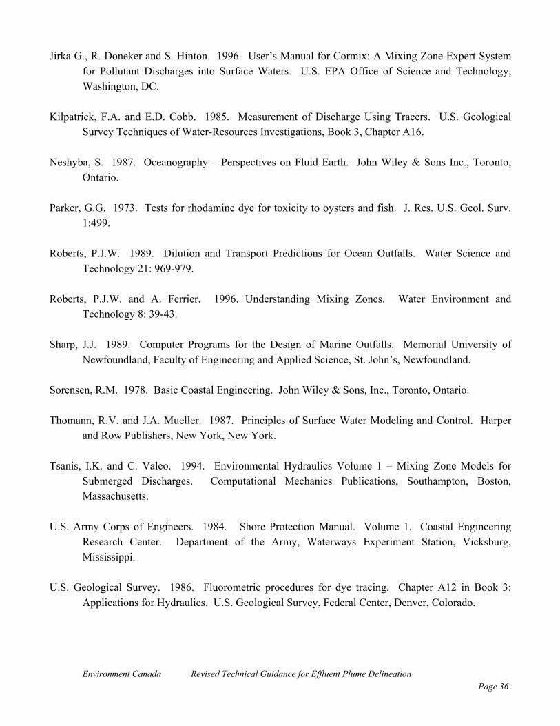
Environment Canada Revised Technical Guidance for Effluent Plume DelineationPage 36
Jirka G., R. Doneker and S. Hinton. 1996. User’s Manual for Cormix: A Mixing Zone Expert Systemfor Pollutant Discharges into Surface Waters. U.S. EPA Office of Science and Technology,Washington, DC.
Kilpatrick, F.A. and E.D. Cobb. 1985. Measurement of Discharge Using Tracers. U.S. GeologicalSurvey Techniques of Water-Resources Investigations, Book 3, Chapter A16.
Neshyba, S. 1987. Oceanography – Perspectives on Fluid Earth. John Wiley & Sons Inc., Toronto,Ontario.
Parker, G.G. 1973. Tests for rhodamine dye for toxicity to oysters and fish. J. Res. U.S. Geol. Surv.1:499.
Roberts, P.J.W. 1989. Dilution and Transport Predictions for Ocean Outfalls. Water Science andTechnology 21: 969-979.
Roberts, P.J.W. and A. Ferrier. 1996. Understanding Mixing Zones. Water Environment andTechnology 8: 39-43.
Sharp, J.J. 1989. Computer Programs for the Design of Marine Outfalls. Memorial University ofNewfoundland, Faculty of Engineering and Applied Science, St. John’s, Newfoundland.
Sorensen, R.M. 1978. Basic Coastal Engineering. John Wiley & Sons, Inc., Toronto, Ontario.
Thomann, R.V. and J.A. Mueller. 1987. Principles of Surface Water Modeling and Control. Harperand Row Publishers, New York, New York.
Tsanis, I.K. and C. Valeo. 1994. Environmental Hydraulics Volume 1 – Mixing Zone Models forSubmerged Discharges. Computational Mechanics Publications, Southampton, Boston,Massachusetts.
U.S. Army Corps of Engineers. 1984. Shore Protection Manual. Volume 1. Coastal EngineeringResearch Center. Department of the Army, Waterways Experiment Station, Vicksburg,Mississippi.
U.S. Geological Survey. 1986. Fluorometric procedures for dye tracing. Chapter A12 in Book 3:Applications for Hydraulics. U.S. Geological Survey, Federal Center, Denver, Colorado.

Environment Canada Revised Technical Guidance for Effluent Plume DelineationPage 37
Williams, B.L. 1985. Ocean Outfall Handbook – A manual for the planning, investigation, design andmonitoring of ocean outfalls to comply with water quality management objectives. NationalWater and Soil Conservation, New Zealand.
Wood, I., R. Bell and D. Wilkinson. 1993. Ocean Disposal of Wastewater. World Scientific PublishingCompany, New Jersey.