ROLE OF QUANTUM CORRELATIONS IN QUANTUM COMMUNICATION NETWORKS

By

TAMOGHNA DAS

PHYS08201105007

Harish-Chandra Research Institute, Allahabad

A thesis submitted to the

Board of Studies in Physical Sciences

In partial fulfillment of requirements

for the Degree of

DOCTOR OF PHILOSOPHY of

HOMI BHABHA NATIONAL INSTITUTE

August, 2017

STATEMENT BY AUTHOR

This dissertation has been submitted in partial fulfillment of requirements for an

advanced degree at Homi Bhabha National Institute (HBNI) and is deposited in the

Library to be made available to borrowers under rules of the HBNI.

Brief quotations from this dissertation are allowable without special permission,

provided that accurate acknowledgement of source is made. Requests for permission

for extended quotation from or reproduction of this manuscript in whole or in part

may be granted by the Competent Authority of HBNI when in his or her judgment the

proposed use of the material is in the interests of scholarship. In all other instances,

however, permission must be obtained from the author.

Tamoghna Das

DECLARATION

I, hereby declare that the investigation presented in the thesis has been carried out by

me. The work is original and has not been submitted earlier as a whole or in part for a

degree / diploma at this or any other Institution / University.

Tamoghna Das

List of Publications arising from the thesis

Journal

1. “Multipartite dense coding versus quantum correlation: Noise inverts relative capability of information transfer”, Tamoghna Das, R. Prabhu, Aditi Sen(De), and Ujjwal Sen, Phys. Rev. A, 2014, Vol. 90, 022319.

2. “Distributed quantum dense coding with two receivers in noisy environments”,

Tamoghna Das, R. Prabhu, Aditi Sen(De), and Ujjwal Sen, Phys. Rev. A, 2015, Vol. 92, 052330.

3. “Superiority of photon subtraction to addition for entanglement in a multimode

squeezed vacuum”, Tamoghna Das, R. Prabhu, Aditi Sen(De), and Ujjwal Sen, Phys. Rev. A, 2016, Vol. 93, 052313.

Preprint

4. “Deterministic Quantum Dense Coding Networks”, Saptarshi Roy, Titas Chanda, Tamoghna Das, Aditi Sen(De), and Ujjwal Sen, arXiv:1707.02449 [quant-ph].

Further Publications of candidate not used substantially in this thesis

Journal

5. “Reducing computational complexity of quantum correlations”, Titas Chanda, Tamoghna Das, Debasis Sadhukhan, Amit Kumar Pal, Aditi Sen(De), and Ujjwal Sen, Phys. Rev. A, 2015, Vol. 92, 062301.

6. “Statistics of leading digits leads to unification of quan- tum correlations”,

Titas Chanda, Tamoghna Das, Debasis Sadhukhan, Amit Kumar Pal, Aditi Sen(De), and Ujjwal Sen, Europhys. Lett., 2016, Vol. 114, 30004 (Highlights).

7. “Distribution of Bell-inequality violation versus multiparty-quantum-

correlation measures”, Kunal Sharma, Tamoghna Das, Aditi Sen(De), and Ujjwal Sen, Phys. Rev. A, 2016, Vol. 93, 062344.

8. “Generalized Geometric Measure of Entanglement for Multiparty Mixed

States”, Tamoghna Das, Sudipto Singha Roy, Shrobona bagchi, Avijit Mishra, Aditi Sen(De), and Ujjwal Sen, Phys. Rev. A, 2016, Vol. 94, 022336.

9. “Static and dynamical quantum correlations in phases of an alternating-field XY model”, Titas Chanda, Tamoghna Das, Debasis Sadhukhan, Amit Kumar Pal, Aditi Sen(De), and Ujjwal Sen, Phys. Rev. A, 2016, Vol. 94, 042310.

10. “Canonical distillation of entanglement”, Tamoghna Das, Asutosh Kumar, Amit Kumar Pal, Namrata Shukla, Aditi Sen(De), and Ujjwal Sen, Phys. Lett.. A, 2017, Vol. 381, 41. Accepted

11. “Quantum discord and its allies: a review”, Anindita Bera, Tamoghna Das, Debasis Sadhukhan, Sudipto Singha Roy, Aditi Sen(De), and Ujjwal Sen, arXiv:1703.10542 [quant-ph], to be published in Rep. Prog. Phys.

12. “Emergence of entanglement with temperature and time in factorization-

surface states”, Titas Chanda, Tamoghna Das, Debasis Sadhukhan, Amit Kumar Pal, Aditi Sen(De), and Ujjwal Sen, arXiv:1705.09812 [quant-ph], to be published in Phys. Rev. A.

Preprint 13. “Activation of nonmonogamous multipartite quantum states”, Saptarshi Roy,

Tamoghna Das, Asutosh Kumar, Aditi Sen(De), and Ujjwal Sen, arXiv:1608.06914 [quant-ph].

14. “Scale-invariant freezing of entanglement”, Titas Chanda, Tamoghna Das,

Debasis Sadhukhan, Amit Kumar Pal, Aditi Sen(De), and Ujjwal Sen, arXiv:1610.00730 [quant-ph].

15. “Phase boundaries in alternating field quantum XY model with Dzyaloshinskii-Moriya interaction: Sustainable entanglement in dynamics”, Saptarshi Roy, Titas Chanda, Tamoghna Das, Debasis Sadhukhan, Aditi Sen(De), and Ujjwal Sen, arXiv:1710.11037 [quant-ph].

Conferences

1. Meeting on Quantum Information Processing and Applications (QIPA-13), 2-8 December 2013, held in Harish-Chandra Research Institute, Allahabad, India. �

2. International Program on Quantum Information (IPQI-14), 22 Febuary-02

March 2014, held in Institute of Physics (IOP), Bhubaneshwar, India. Contributed poster entitled “Multiparty Dense Coding vs. Quantum Correlation: Noise Inverts Relative Capability of Information Transfer”.

3. One day QIC workshop, 13 November 2014, Harish-Chandra Research Institute, India. Oral presentation on “Canonical Distillation of Entanglement”.

4. Young Quantum-2015 (YouQu-15), 23-26 February 2015, Harish-Chandra

Research Institute, India. Oral presentation on “Distributed Quantum Dense Coding in Noisy Scenario”.

5. International Conference on Quantum Foundations (ICQF-15), 30 November-

04 December 2015, held in NIT Patna, India. Contributed poster entitled “Distributed Quantum Dense Coding in Noisy Environments”.

6. Meeting on Quantum Information Processing and Applications (QIPA-15), 7-

13 December 2015, held in HRI Allahabad, India. Contributed two posters entitled “Regional and global quantum correlations: their interrelation and use”, and “Asking quantum correlation about their monogamy score”

7. Joint IAS-ICTP school on Quantum Information, NTU, Singapore, January

2016. Contributed poster entitled “Distributed Quantum Communication”. 8. Young Quantum-2017 (YouQu-17), 27 February- 01 March 2017, Harish-

Chandra Research Institute, India. Contributed poster entitled “Activation of Nonmonogamous Multipartite Quantum States”.

9. Advanced School and Workshop on Quantum Science and Quantum Technologies, ICTP, Trieste, Italy, January 2017. Oral presentation on “ Multipartite entanglement measure and its application in quantum communication”.

Others

1. Served as a Tutor, Classical Mechanics course, Aug-Dec Semester, 2014. 2. Served as a Tutor, Quantum Information and Computation course, Jan-May

Semester, 2016. 3. Members of local organizing committee of Meeting on Quantum Information

Processing and Applications (QIPA-2013, QIPA-2015) and Young Quantum Meet (YouQu-15, YouQu-17) at Harish-Chandra Research Institute, 2013, 2015 and 2017.

Tamoghna Das

ACKNOWLEDGEMENTS

It was hardly possible for me to complete this thesis without the precious support of a number ofpeople. First of all, I want to thank my Ph.D supervisor, Prof. Aditi Sen(De), for her continuous guidanceand support throughout my Ph.D. tenure. And it was her deep believe on me, as well as her supervision,continuous moral support, tremendous e�orts which make me able to circumvent all the shortcomingsthat I have and make me able to do research. I am extremely lucky and it is an honor for me that I havesuch a supervisor.

I want to thank Prof. Ujjwal Sen for his incessant support, academic and moral steering, constantencouragement and constructive criticism which gave a positive direction to this thesis, and many projectsgot new motivations due to him. I am also thankful to him due to the “Numerical methods” course, hetaught us and explaining the logic and methodology behind the numerical techniques and for a instantdemonstration of writing, compiling and running code in the classroom, making a transition of a theoreticalclass to a practical one. I am also thankful to Prof. Arun Kumar Pati for his encouragements, cool cheerfulnature, and illuminating me with his vast knowledge and stimulating ideas every time. I want to thankall the faculty members of our "Quantum Information and Computation" group to make our group mosthappening group, and for encouraging us to arrange many group seminars, conferences, workshops andmost importantly many non-academic tours in many places of this country.

I express my sincere gratitude to all faculty members of HRI for imparting unparalleled courses onphysics and providing me many useful suggestions about physics and life. I am thankful to Prof. BiswarupMukhopadhyaya and Anshuman Maharana and the other members of my thesis advisory committee fortheir assistance during my extension talk and beyond. I acknowledge the constant support from the peoplein the computer center, especially Mr. Rajiv, Mr. Ravi and Mr. Chandan for their humble nature, attendinginstantly any problems in the computer and help me a lot to know the installation of any new package ina computer. I also extend my thank to the HPC cluster facility at HRI, on which numerical simulationsrelevant to this thesis were done. I must thank the administrative o�cers and other employees of the wholeadministration at HRI, Allahabad and HBNI, Mumbai for their sincere help and support.

I acknowledge the discussions which I have made during our course work, especially with Sauri andSoumyadeep. Without their help, I could not even manage to learn many parts of quantum mechanics,statistical mechanics, general theory of relativity, condensed matter physics. I could not forget thememorable times that I have spent with the entire integrated 2011 batch of HRI during our visits toIGCAR, Kalapakkam and NISER, Bhubneswar for the experimental projects. I also want to thank myfriends, Samrat and Titas and also to Atri Da for teaching me all the necessary stu�s in C and C++programming in greater details, and also for spending a significant amount of their precious time for me tosolve my own problems. And during my Ph.D life, I was also enlightened by the constructive discussions,and an immense amount of help that I got from the group-members, especially, from Prof. R. Prabhu,Amit da, Manab da, Anindya da, Debraj da, Himadri da, Samya da, Utakarsh, Avijit da, Shrobona di,Asutosh, Uttam, Debasis da, Debasis Shadhukhan, Sudipto, Anindita, Titas, Saptarshi and Sreetama. Allthe discussions during QuIC dinner and arXiv flashback, walking at night at HRI and other informalmoments with them and other members of the group immensely help me to get the knowledge that Icurrently have on the subject.

Staying in a hostel away from home for the first time never turned out to be a di�cult task, due to myfriends at HRI, juniors and seniors and all of my group members including my supervisor. With them, Ispent a lot of time, discussing the problems in my life and in physics, having many dinner parties togetherinside and outside the campus. I would like to thank Samrat, Sarosh, Sauri, Soumyadeep, Saikat, Uttam,Krishna-Mohan, Abhishek Joshi, Sourav Niyogi, Narayan Rana, Taushif, Subhroneel, Utkarsh, Amit da,Debraj da, Titas, Sourav Bhattacharya, Debasis Sadhukhan, Sudipto, Anindita, Kunal, Saptarshi for that.Playing games including the daily badminton, weekend cricket in the community center and in the fieldwas a very exciting for me, as they help me to relax and give me a new enthusiasm to work towards mythesis. I would also like to thank the people working at mess, pantry and guest house to serve nice foods,even at mid-night and also to all the members of the security agency "Fighting four" and "Warriors" formaking HRI, a secure place to live.

I cannot forget the trips which I have made with the group members in my entire Ph.D tenure with aregular interval of time. They were such a nice and relaxing moments which we spent together, withinnature in the dark night of Binsar, in forests like Sundarban, Bharatpur, Shivpuri, in waterfalls at Ranehand Rajdari and Debdari, watching snow peaks from Ranikhet and Koushani, historical places like Agra,Khajuraho, Jaipur, Jhansi and Sarnath. Thanks to Amit da, Aditi di and Ujjwal da and others for arrangingthose trips and make the entire plan of travel and for reminding us the necessary stu�s that one should notmiss for a trip, for being the guide and for making all the trips successful. Spending times with all thegroup members in various places with regular interval of time help us to unite our group, increase bondingbetween each other and teach us how to overcome di�cult times in life and help other group members indi�cult time. All of these trips help me a lot to pursue the Ph.D and complete my thesis.

At the end, I have no words to express my gratitude to my parents, elder brother, sister-in-law and alsoto the teachers from my school and from the college, for their sumptuous support, care, a�ection, frommy early days of schools till today. Their priceless encouragement make me able to complete the Ph.Ddegree. I am also very much thankful to the lovely daughter of my supervisor, S(n)ajh (Anusyuta Sen),for her delighting nature and serious advice in a childish tone which makes my entire day.

ii

Contents

SYNOPSIS vii

LIST OF FIGURES xvi

LIST OF TABLES xxii

1 Introduction 1

2 Quantum Correlation Measures 72.1 Bipartite entanglement . . . . . . . . . . . . . . . . . . . . . . . . . . . . . . . . . . . 72.2 Measures of bipartite entanglement . . . . . . . . . . . . . . . . . . . . . . . . . . . . 8

2.2.1 Entanglement entropy . . . . . . . . . . . . . . . . . . . . . . . . . . . . . . . 92.2.2 Entanglement of formation and Concurrence . . . . . . . . . . . . . . . . . . . 92.2.3 Negativity and Logarithmic Negativity . . . . . . . . . . . . . . . . . . . . . . 10

2.3 Information theoretic quantum correlation measures . . . . . . . . . . . . . . . . . . . . 112.3.1 Quantum Discord . . . . . . . . . . . . . . . . . . . . . . . . . . . . . . . . . . 112.3.2 Quantum work deficit . . . . . . . . . . . . . . . . . . . . . . . . . . . . . . . . 13

2.4 Multipartite measures of entanglement . . . . . . . . . . . . . . . . . . . . . . . . . . . 142.4.1 Distance-based measure . . . . . . . . . . . . . . . . . . . . . . . . . . . . . . 152.4.2 Monogamy-based measure . . . . . . . . . . . . . . . . . . . . . . . . . . . . . 16

3 Dense Coding Protocol Involving Multiple Senders and a Single Receiver 193.1 Dense Coding protocol in a noiseless scenario . . . . . . . . . . . . . . . . . . . . . . . 19

3.1.1 Dense coding protocol for singlet . . . . . . . . . . . . . . . . . . . . . . . . . 203.1.2 DC for arbitrary shared state . . . . . . . . . . . . . . . . . . . . . . . . . . . . 213.1.3 Dense coding protocol involving multiple senders and a single receiver . . . . . 24

3.2 Dense coding capacity in presence of noise . . . . . . . . . . . . . . . . . . . . . . . . 253.2.1 Mathematical description of noise . . . . . . . . . . . . . . . . . . . . . . . . . 253.2.2 Examples of noisy quantum channels . . . . . . . . . . . . . . . . . . . . . . . 263.2.3 Capacity of DC for covariant noise . . . . . . . . . . . . . . . . . . . . . . . . . 29

iii

Contents

4 Multipartite Dense Coding vs. Quantum Correlations 314.1 Connection of QC measures with capacity DC in a noiseless scenario . . . . . . . . . . 32

4.1.1 Connection with genuine multiparty entanglement measure . . . . . . . . . . . . 324.1.2 Connection with monogamy based measures . . . . . . . . . . . . . . . . . . . 34

4.2 Multiparty DC vs. QC for multiparty mixed state . . . . . . . . . . . . . . . . . . . . . 364.3 Relation of multiparty QC measures with capacity of DC in presence of noise . . . . . . 39

4.3.1 Fully correlated Pauli channel . . . . . . . . . . . . . . . . . . . . . . . . . . . 394.3.2 Local depolarizing channel . . . . . . . . . . . . . . . . . . . . . . . . . . . . . 43

4.4 In closing . . . . . . . . . . . . . . . . . . . . . . . . . . . . . . . . . . . . . . . . . . 45

5 Distributed Quantum Dense coding 475.1 Chain rule of Mutual information . . . . . . . . . . . . . . . . . . . . . . . . . . . . . . 475.2 Locally accessible information . . . . . . . . . . . . . . . . . . . . . . . . . . . . . . . 48

5.2.1 Information gain in a single measurement . . . . . . . . . . . . . . . . . . . . . 505.2.2 Information gain in successive measurements . . . . . . . . . . . . . . . . . . . 52

5.3 Distributed quantum dense coding . . . . . . . . . . . . . . . . . . . . . . . . . . . . . 555.3.1 Distributed dense coding capacity . . . . . . . . . . . . . . . . . . . . . . . . . 565.3.2 Distributed DC with four-qubit GHZ state . . . . . . . . . . . . . . . . . . . . . 57

5.4 Distributed DC in presence of noisy quantum channels . . . . . . . . . . . . . . . . . . 615.4.1 Upper bound on LOCC-DC for arbitrary noisy channel . . . . . . . . . . . . . . 615.4.2 LOCC-DC capacity under covariant noise . . . . . . . . . . . . . . . . . . . . . 63

5.5 Examples of noisy quantum channels . . . . . . . . . . . . . . . . . . . . . . . . . . . . 655.5.1 Amplitude Damping Channel . . . . . . . . . . . . . . . . . . . . . . . . . . . 665.5.2 Phase Damping Channel . . . . . . . . . . . . . . . . . . . . . . . . . . . . . . 685.5.3 Pauli Noise: A Covariant Channel . . . . . . . . . . . . . . . . . . . . . . . . . 68

5.6 Connecting Multipartite Entanglement with LOCC-DC . . . . . . . . . . . . . . . . . . 705.6.1 Connection of multiparty entanglement with noisy LOCC-DC . . . . . . . . . . 74

5.7 In closing . . . . . . . . . . . . . . . . . . . . . . . . . . . . . . . . . . . . . . . . . . 75

6 Photon Subtracted State is More Entangled than Photon Added State 776.1 N-mode squeezed vacuum state . . . . . . . . . . . . . . . . . . . . . . . . . . . . . . . 78

6.1.1 Another form of NMSV state . . . . . . . . . . . . . . . . . . . . . . . . . . . . 806.1.2 Two-mode squeezed vacuum state . . . . . . . . . . . . . . . . . . . . . . . . . 826.1.3 Four-mode squeezed vacuum state . . . . . . . . . . . . . . . . . . . . . . . . . 83

6.2 Preparation of FMSV state . . . . . . . . . . . . . . . . . . . . . . . . . . . . . . . . . 836.3 Photon-added and -subtracted FMSV state . . . . . . . . . . . . . . . . . . . . . . . . . 856.4 Comparison of entanglement enhancement between photon addition and subtraction . . . 86

6.4.1 Photon added and subtracted with one player mode . . . . . . . . . . . . . . . . 876.4.2 Behavior of entanglement of photon-added and -subtracted states with two player

modes . . . . . . . . . . . . . . . . . . . . . . . . . . . . . . . . . . . . . . . . 946.5 Comparison of logarithmic negativity between two-mode and four-mode states . . . . . . 996.6 Measure of non-classicality in continuous variable systems . . . . . . . . . . . . . . . . 1016.7 In Closing . . . . . . . . . . . . . . . . . . . . . . . . . . . . . . . . . . . . . . . . . . 104

iv

Contents

7 Summary and Future Directions 1057.1 Summary of the Thesis . . . . . . . . . . . . . . . . . . . . . . . . . . . . . . . . . . . 1067.2 Future Directions . . . . . . . . . . . . . . . . . . . . . . . . . . . . . . . . . . . . . . 107

Bibliography 110

v

Contents

vi

SYNOPSIS

Information transmission between multiple senders and multiple receivers plays an important role in

our day-to-day life. The emergence of technologies over the last decades revolutionize the way we

communicate. For example, the hand written letters have been replaced by phone-calls, emails, video-

chats etc while mass communication also has changed its form from newspaper, mass-gathering to internet

version of them. The existing communication systems can broadly be divided into two categories – the

communication with security (cryptography) and without securities. In both the cases, it was proven

that quantum mechanical laws provide advantages over their classical counterparts [1–4]. Moreover, in

a quantum domain, there can be a task which deals with transferring quantum states between two distant

locations [5]. During last two decades, it was also found that the common ingredient which makes all

these protocols successful is the shared quantum correlation aka entanglement [6] between the sender

and the receiver. Apart from the communication schemes, entanglement also plays a crucial role in other

technological tasks like error correction [7, 8], and one way quantum computation [9]. In last decade, it

has also been established that in physical systems, entanglement as well as other quantum correlations in

nearest and next nearest neighbor spins of ground and thermal states can be useful to detect co-operative

quantum phenomena like quantum phase transitions, thermal transitions [10, 11].

Let us now concentrate only on classical information transmission (without security) via quantum

states and its possible connection with quantum correlation measures. The usual way to transmit classical

information is to encode the message in the string of classical bits of 0 and 1, and to send one bit in this

manner, one requires two distinguishable objects or two orthogonal states or two dimensional systems. In

1992, Bennett and Wiesner [4] showed that if the sender and the receiver share a maximally entangled

state, two bits of classical information can be communicated using only a single quantum bit (qubit),

i.e., a two-dimensional quantum system by performing unitary operators on sender’s part. It is then sent

through a shared quantum channel followed by a measurement on receiver’s side. The process is known as

quantum dense coding or super dense coding [4]. Note that the sender and the receiver, having no shared

entanglement, requires four-dimensional system for sending two classical bits. For an arbitrary shared

bipartite quantum state, the capacity of dense coding (DC) can be obtained by performing optimizations

over all possible unitary encodings, the probability of encodings, and over all quantum mechanically

allowed measurements performed by the receiver. The later optimization over measurements for a given

set of states is already obtained by Holevo in 1973 [12]. In particular, it was shown that the information

Contents

accessible to the receiver upon measurements, is upper bounded by a quantity, known as a Holevo

quantity, which can be achieved assymptotically [13, 14]. Hence, in the two-party scenario, the DC

capacity reduces to the maximization of the Holevo quantity over all possible encodings and probabilities.

Such optimizations can be performed analytically and hence the capacity of DC is already known in this

scenario [15](see also [16–20]). It turns out that for pure bipartite states, the DC capacity increases with

the increase of shared bipartite entanglement among the sender and the receiver [6].

The usefulness of communication protocols becomes more prominent, when they involve multiple

senders and multiple receivers. On the other hand, the transmission channel in a realistic situation

can not be kept completely isolated from the environment, and hence noise almost certainly acts on

the encoded parts of the senders’ subsystems at the time of sending them through quantum channels.

Therefore, extending the DC protocol with several senders and several receivers in the presence of noise

is an interesting and important problem in communication theory. The DC capacities involving multiple

senders and a single as well as two receivers are obtained for a noiseless case [21, 22], and also recently

for a specific noisy channels [23–26] with a single receiver.

In a multiparty domain, the connection of multiparty entanglement or quantum correlation measures

with multiparty DC capacity in both noiseless and noisy scenario is still an open question. The challenges

behind establishing such connection are as follows: (1) the noisy DC capacity from many senders to more

than one receiver is not known; (2) there is no unique measure of multiparty entanglement or quantum

correlation, even for pure states. In the proposed thesis, we will overcome both the di�culties. We will find

a compact form of DC capacities for multiple senders and two receivers for noisy channels and the second

one is settled by considering two computable multiparty measures based on the geometry of the state space

of multiparty quantum states [27–29] and the concept of monogamy of quantum correlations [30, 31].

In the finite dimensional case (mainly qubit system), there are some drawbacks in the possible im-

plementation of quantum communication networks in the laboratory [32–35]. However, those drawbacks

can be overcome by considering continuous variable (CV) systems. In recent times, the classical in-

formation transfer by using a quantum channel has been successfully investigated both theoretically and

experimentally, in CV systems, especially in Gaussian states [36–41]. However, it has been discovered

that there are several protocols which can not be implemented using Gaussian states with Gaussian op-

erations. Examples include entanglement distillation [42, 43], measurement-based universal quantum

computation [44, 45], teleportation [46, 47], and quantum error correction [48]. The increasing impor-

tance of non-Gaussian states have led to the discovery of several mechanisms to create such states in the

laboratory [49, 50]. An important one is adding and subtracting photons, when the initial state is the

viii

Contents

squeezed vacuum state [51–54]. In the proposed thesis, we consider the four-mode squeezed vacuum

(FMSV) state as input and deGaussify it by adding and subtracting photons in di�erent modes.

We state below the main results, obtained in the proposed thesis.

• We established a connection between multiparty quantum correlation measures and multiparty DC

capacity with arbitrary number of senders and a single receiver [21] in a noiseless scenario [55].

According to the usefulness in DC protocol, we obtained a relative hierarchy among arbitrary

multiqubit pure states and the generalized Greenberger-Horne-Zeilinger (gGHZ) [56] states having

an equal amount of multipartite entanglement.

• In presence of covariant noise in the senders subsystem, we derived an upper bound on the capacity

of classical information transfer between multiple senders and two receivers (distributed DC) [57],

where the receivers are situated in distant locations and can only perform local operations and

classical communication (LOCC) [6].

• We found that the presence of su�cient amount of noise, in the quantum channels, can invert the

relative capability of information transfer for two states (the gGHZ state and the arbitrary multiparty

states) with the same multiparty quantum correlation content [55,57]. The gGHZ state turns out to

be more advantageous compared to other three-qubit pure states, having same genuine multiparty

entanglement in case of DC scheme with more than one receiver.

• A potential physical system in which quantum communication protocols have successfully been

implemented is the class of continuous variable systems. Towards such possible realizations, we

have investigated the entanglement patterns of photon-added and -subtracted four-mode squeezed

vacuum states [58]. We found that these non-Gaussian states are highly entangled compared to the

Gaussian states.

The content of the thesis is divided into seven Chapters.

In Chapter 1 (Introduction), we will discuss about the role of communication network in our day-to-

day life and its rapid development over the last few decades. We will also discuss the role of quantum

correlations in these revolutionary quantum communication schemes. Chapter 2 (Quantum Correlation

Measures), discusses the basic definitions of bipartite entanglement measures and other quantum corre-

lation measures [6], independent of entanglement. Some of the basic measures of multipartite quantum

correlations which we will use in the proposed thesis will also be discussed [27,28,30,31] in this chapter.

In Chapter 3 (Dense Coding Protocol Involving Multiple Senders and a Single Receiver), we first describe

ix

Contents

the dense coding protocol for transferring classical information [15] by using an arbitrary shared bipartite

quantum state. We then evaluate the DC capacity for arbitrary bipartite states and extend it to multiple

senders and single receiver [21]. Then I will move to a discussion of DC protocol when there is a noise

in the transmission channel [23, 24].

A connection between multipartite quantum correlation measures of the shared state and the multiparty

DC capacity involving several senders and a single receiver will be reported in Chapter 4 (Multipartite

Dense Coding vs. Quantum Correlations) [55]. In particular, we show that for the noiseless channel, if

multipartite quantum correlation of an arbitrary multipartite state with arbitrary number of qubits is the

same as that of the corresponding generalized Greenberger-Horne-Zeilinger state [56], then the multipartite

dense coding capability of former is the same or better than that of the gGHZ state. The result is generic

as it holds for the genuine multiparty entangled measure, known as generalized geometric measure [28],

as well as for the squared-concurrence [30] and discord monogamy scores [31]. Interestingly, we also

analytically prove that the relative capability of classical information transfer between the gGHZ and

arbitrary states having the same multiparty quantum correlation content, can be inverted by administering

a su�cient amount of noise.

In Chapter 5 (Distributed Quantum Dense Coding), we will first discuss the dense coding protocol

between an arbitrary number of senders and two receivers. We will then investigate [57] the e�ects of noisy

channels in this scenario and derive an upper bound on the multipartite DC capacity which is tightened

in case of a specific noisy channel, namely the covariant noisy channel [59]. Finally, we also establish a

relation between the genuine multiparty entanglement of shared state and the capacity of distributed dense

coding using that state, both in the noiseless and the noisy scenarios [57].

Upto now, we have investigated the role of quantum correlation measures in quantum communication

schemes in finite dimensional systems. Physical systems that mimic these finite dimensional quantum states

include photons with e.g., polarization degrees of freedom, internal levels of ions etc. Such systems have

some drawbacks [32–35] which can be overcome by using continuous variable (CV) systems [37,39,60].

In CV systems, entanglement are created in the position and momentum variables. Towards creating

highly entangled states for possible implementation of quantum communication protocols, in Chapter 6

(Photon Subtracted State is More Entangled than Photon Added State), we report entanglement patterns

of four-mode squeezed vacuum states, under addition and subtraction of photons in di�erent modes [58].

We show that entanglement contents of these photon-added and -subtracted states are higher than the

initial four mode squeezed vacuum states.

In Chapter 7 (Summary and Future Directions), we will discuss brief summary of all the results

x

Contents

presented in the thesis and some of the future directions which include building of quantum communication

network in a deterministic manner [61], which will be easy to realize in experiments.

We believe that the results obtained in the proposed thesis will be step forward to build a quantum

communication network in a realistic scenario. It also sheds light on the status of shared multipartite

quantum correlations in this network.

xi

Contents

xii

List of Figures

4.1 GGM vs. multipartite DC capacity. GGM is plotted as the ordinate while multipartiteDC capacity is plotted as the abscissa for 105 randomly chosen three-qubit pure states,according to the uniform Haar measure over the corresponding space (blue triangles). Thered line represents the generalized GHZ states. There is a set of states for which, if thecapacity matches with a gGHZ state, then their GGMs are also equal. For the remainingstates, if the capacity is equal to a gGHZ state, its GGM is bounded above by that of thegGHZ state. Note that the range of the horizontal axis is considered only when the statesare dense codeable. The quantities represented on both the axes are dimensionless. Weare considering the case where the post-encoded states are sent through noiseless channels. 34

4.2 Left: Tangle (vertical axis) vs. multiparty DC capacity (horizontal axis) for randomlygenerated three-qubit pure states (blue triangles). Right: Discord monogamy score (ver-tical axis) vs. DC capacity (horizontal axis) for the same states. In both the cases, thegGHZ states give the boundary (red line). The capacity is dimensionless, while the tan-gle and discord monogamy score are measured in ebits and bits, respectively. All otherconsiderations are the same as in Fig. 4.1. . . . . . . . . . . . . . . . . . . . . . . . . . 36

4.3 Discord monogamy score vs. multipartite DC capacity for Haar uniformly generatedrank-2 three-qubit states. The red line represents the gGHZ states. About 1.85% of therandomly generated states lie below the red line, and are represented by blue triangles.The remaining, represented by green “three o’clock” circles, lie above the red line. Thehorizontal axis is dimensionless while the vertical one is measured in bits. . . . . . . . . 38

4.4 Discord monogamy score and the raw DC capacity are plotted against the mixing param-eter p, for the rank-8 state, ⇢8 = (1 � p)⇢ + p

8I . Here ⇢ = q|GHZihGHZ| + (1 �

q)|GHZ0ihGHZ

0|. Each value of q provides a curve, and we present several exemplary

curves in the figure. All the quantities plotted are dimensionless, except �D, which ismeasured in bits. . . . . . . . . . . . . . . . . . . . . . . . . . . . . . . . . . . . . . . 39

xvii

List of Figures

4.5 GGM (vertical axis) vs. the raw DC capacity (horizontal axis) under the fully correlatedPauli channel, when the shared state is an arbitrary three-qubit pure state (orange squares,green circles, and blue triangles) or the gGHZ state (red line). For figure (a), we chooseq0 = q3 = 0.485, and q1 = q2 = 0.015 as noise parameters for the arbitrary as well asthe gGHZ state, this corresponds to the Case 1. And for figure (b), we choose {qi} asq0 = 0.93, q1 = 0.01, q2 = 0.02, q3 = 0.04, corresponds to the Case 2 in the discussion.We randomly (Haar uniformly) generate 105 three-qubit pure states. Both the axes aredimensionless. The vertical line at the C

noisyc = 2/3 helps to readily read out the actual

capacity from the raw capacity. . . . . . . . . . . . . . . . . . . . . . . . . . . . . . . . 414.6 Figure (a), Tangle (vertical axis) vs. the raw DC capacity (horizontal axis) under the

fully correlated Pauli channel, for randomly (Haar uniformly) generated three-qubit purestates (blue triangles) and the gGHZ states (red line). Figure (b) Discord monogamy score(vertical axis) vs. noisy DC capacity (horizontal axis) for the same set of states. Wechoose q0 = q3 = 0.485, and q1 = q2 = 0.015 as noise parameters for the arbitrary aswell as for the gGHZ state, this corresponds to the Case 1. The noisy DC capacity isdimensionless, while the tangle and discord monogamy score are measured in ebits andbits, respectively. The vertical line at the Cnoisy

c = 2/3 is to identify the classical domainof capacity. . . . . . . . . . . . . . . . . . . . . . . . . . . . . . . . . . . . . . . . . . 43

4.7 DC capacity vs. noise for various choices of ↵ in the gGHZ state. In the top panel,the capacity of DC is plotted against the noise of the depolarizing channel, while in thebottom one, the DC capacity is plotted with respect to the noise in the fully correlatedPauli channel, for the gGHZ state. Di�erent curves correspond to di�erent values of ↵.The vertical axis starts from 2/3, below which the states are not dense codeable. Thestates remain dense codeable in the presence of moderate to high Pauli noise while this isnot the case for the uncorrelated depolarizing channel. The horizontal axes are measuredin bits. All other quantities are dimensionless. . . . . . . . . . . . . . . . . . . . . . . . 44

4.8 (Color online.) GGM vs. the raw DC capacity, Cnoisyuc , in the presence of the uncorrelated

noise. See text for further details. Both axes represent dimensionless quantities. Thevertical line at Cnoisy

uc = 2/3 again helps to read the actual capacity from the raw capacity. 454.9 Schematic diagram of the change of status of the gGHZ state in comparison to other

multipartite states with respect to multipartite DC capacity in the presence of noise. Thecomparison has been made with the states which posses same amount of multipartitequantum correlations as the gGHZ state. The results obtained in this paper shows thatthe gGHZ state is more robust against noise as compared to arbitrary states for the densecoding protocol. This is independent of the fact whether the noise in the system is fromthe source or in the channel after the encoding. . . . . . . . . . . . . . . . . . . . . . . 46

5.1 The LOCC protocol of obtaining information about the message x, which occurs withprobability px, when Alice and Bob share an ensemble {px, ⇢xAB}. First Alice initiates themeasurement on her part of the ensemble and communicates the result to Bob. Dependingon the Alice’s outcome, Bob chooses and performs another measurement on the sharedpost measurement ensemble and communicates his outcome. The process goes on untilthey gather maximal information about the ensemble. . . . . . . . . . . . . . . . . . . 49

xviii

List of Figures

5.2 A schematic diagram of the DC protocol of two receivers. An (N + 2)-party quantumstate, ⇢S1S2...SNR1R2 , is shared between N senders, S1, S2, . . . , SN , and two receivers,R1 and R2. We assume that after unitary encoding, the senders, S1, S2, . . . , Sr, send theirpart to the receiver R1 while the rest send their parts to the receiver, R2. To decode, R1

and R2 are only allowed to perform LOCC. . . . . . . . . . . . . . . . . . . . . . . . . 55

5.3 Plots of the quantities a21pf(a1)

log1�p

f(a1)

1+p

f(a1)and 1�a21p

g(a1)log

1�p

g(a1)

1+p

g(a1), which are respec-

tively the left-hand- and right-hand-sides of Eq. (5.116), against a1 and �. The green(gray in print) surface represents the first while the purple (dark in print) one is for thesecond expression. The intersection line (white line) is a1 = 1p

2, for all �. The base axes

are dimensionless, while the vertical axis is in bits. . . . . . . . . . . . . . . . . . . . . 67

5.4 Noiseless case: How does a general four-qubit pure state compare with the gGHZ states?We randomly generate 105 four-qubit pure states uniformly with respect to the correspond-ing Haar measure, and their GGM is plotted as the abscissa while B

LOCC is plotted asthe ordinate. The red curved line represents the gGHZ states. Among the states gener-ated randomly, 47.6% (blue triangles) satisfy both the conditions in Result, 49% (orangesquares) violate either of the conditions, but still falls above the gGHZ line. Green circlesrepresent 3.4% states which violate the conclusion of Result. The line at abscissa equals to2 corresponds to the capacity achievable without prior shared entanglement. The verticalaxis is dimensionless, while the horizontal one is in bits. . . . . . . . . . . . . . . . . . 73

5.5 Noiseless case: Comparison between arbitrary four-qubit pure states and the gGHZ states,with constrained GGM. We randomly generate 105 four-qubit pure states uniformly withrespect to the corresponding Haar measure, and their HV-GGM (EHV) is plotted as theabscissa while BLOCC is plotted as the ordinate. The red curved line represents the gGHZstates. Among the states generated randomly, 0.7% (green circles) states fall below thegGHZ line. Orange squares represent those state whose E

HV is greater than 0.5 (abovethe horizontal line) – they are very few in number, and constitute only 1.2% of totalgenerated random states. The line at abscissa equals to 2 corresponds to the capacityachievable without prior shared entanglement. The vertical axis is dimensionless, whilethe horizontal one is in bits. . . . . . . . . . . . . . . . . . . . . . . . . . . . . . . . . 74

5.6 Fully correlated Pauli noise: The gGHZ states are again better than a significant fractionof states. We plot the GGM as the ordinate and �LOCC

noisy as the abscissa for 105 randomlygenerated four-qubit pure states uniformly with respect to the corresponding Haar measurefor low (figure (a)) and high (figure (b)) full correlated Pauli noise. In figure (a), q0 =

0.93, q1 = 0.01, q2 = 0.02, q3 = 0.04, while in figure (b), we choose q0 = 0.485, q1 =

0.015, q2 = 0.015, q3 = 0.485. In the presence of high noise, almost all states arebounded by the four-qubit gGHZ states (red curved line). A significant fraction of thegenerated states lie above the gGHZ line even for low noise. It indicates that the gGHZstate is more robust against noise as compared to an arbitrary four-qubit pure state. Thelines at abscissa equals to 2 correspond to the capacity achievable without prior sharedentanglement. The vertical axis is dimensionless, while the horizontal one is in bits. . . . 75

xix

List of Figures

6.1 Schematic description of the preparation of FMSV state in the laboratory. Here |ri and| � ri are two SMSV states with squeezing parameter r, squeezed di�erent quadratureoperators. After passing through the 50 : 50 Beam splitter, it creats the TMSV state, | 2i,given in Eq. (6.37). Then the two modes of TMSV state pass through the another 50 : 50

beam splitter along with the vacuums, resulting the FMSV state as in Eq. (6.41). . . . . 84

6.2 Schematic diagram of choices of player and spectator modes as well as partitions. If wefix the bipartition to be 1 : 234 there are three nontrivial possibilities of choosing a singleplayer in the photon-added and the subtracted FM state. There are the cases (a) - (c),and the number in the square mentioned for each case is the mode at which the photon isadded/subtracted. . . . . . . . . . . . . . . . . . . . . . . . . . . . . . . . . . . . . . . 87

6.3 Behavior of E(| addm1i1:234) and E(| sub

m1i1:234) vs. m1. We add (⇥) and subtract (+) upto

40 photons in (from) the first mode, and calculate entanglement in the 1 : 234 bipartition,when no photons are added (subtracted) in (from) the spectator modes. As shown inthe propositions, entanglement in both the cases increases monotonically with m1 andthey coincide. Here the entanglement is plotted in the unit of ebits while the abscissa isdimensionless. . . . . . . . . . . . . . . . . . . . . . . . . . . . . . . . . . . . . . . . . 90

6.4 (a) Trends of E(| addm2i1:234) and E(| sub

m2i1:234) with the number of photon-added (sub-

tracted) in (from) the second mode. (b) Similar study has been carried out when thethird mode acts as a player. Both the cases reveal that subtraction is better than addition.Ordinates are plotted in the unit of ebits while the abscissas are dimensionless. . . . . . . 92

6.5 Schematic diagram of two di�erent blocks, when a single mode, specifically the firstmode, acts as a player. . . . . . . . . . . . . . . . . . . . . . . . . . . . . . . . . . . . . 93

6.6 (Color online) Plots of entanglements of photon-added and -subtracted states in the 12 : 34

(a) and 13 : 24 (b) bipartitions with m1. The ordinates are plotted in the unit of ebitswhile the abscissas are dimensionless. . . . . . . . . . . . . . . . . . . . . . . . . . . . 94

6.7 (Color online) Plot of convergence of von Neumann entropy, SN (⇢add12,m1), in (a) and

trN (⇢add12,m1) in (b) against N which is the maximum value of n and n

0. We choose threedi�erent values of m1, viz. m1 = 10, 25, 40. We find that for example, for m1 = 40,trace goes to unity and the entropy (entanglement) converges for N � 10. Here thevon-Neumann entropy is measured in the unit of bits and the trace and the abscissas aredimensionless. . . . . . . . . . . . . . . . . . . . . . . . . . . . . . . . . . . . . . . . . 94

6.8 Schematic diagram of four non-trivial possibilities of choosing two modes as players inthe 1 : 234 bipartition. Other choices can be shown as repetitions due to the symmetry ofthe FM state. . . . . . . . . . . . . . . . . . . . . . . . . . . . . . . . . . . . . . . . . 95

xx

List of Figures

6.9 Top panel: Behavior of �E1 (m1,m3) against m1 (horizontal axes) and m3 (vertical axes)when the spectator modes are active, figure(a) both m2 = m4 = 0, figure (b) m2 =

5, m4 = 0 and in figure (c)m2 = m4 = 5. We see that by using fixed number of photonsto the spectators modes, entanglement of photon added state can be enhanced much fasterthan the photon subtracted ones. Bottom panel: Similar behavior of �E1 (m1,m2) againstm1 (horizontal axes) and m2 (vertical axes), when no photons are added in the spectatormode (figure (d)), only one spectator mode is active, m3 = 5, m4 = 0 in figure (e)

and m3 = 0, m4 = 5 in figure (f). We find that the region where photon addition isbetter than the subtraction remains almost constant. All the axes are dimensionless, whileentanglements are plotted in the unit of ebits. . . . . . . . . . . . . . . . . . . . . . . . 96

6.10 Distinct scenarios of the bipartition containing two modes and two player modes in the13 : 24 split (figure (i)) and 12 : 34 (figure (ii)). For the 13 : 24 bipartition there are twopossibilities – (a) first and second as players, (b) first and third as players. In the 12 : 34

split one can chose – (a) first and second as players, (b) first and third as players, and (c)first and forth as player. . . . . . . . . . . . . . . . . . . . . . . . . . . . . . . . . . . . 97

6.11 Role of spectator modes in �E13 in the plane of m1,m2 and m1,m3 when the player modesare active. In (a),m3 = 10 andm4 = 0, while in (b),m3 = m4 = 5. We see that spectatormodes help to enhance entanglement in the photon-added state. In (c) no spectator modeis active, and a positive region emerges around the line m1 = m3 > 14, which can beenhanced more when one spectator mode is active, as shown in (d) where m2 = 4. Allthe axes are dimensionless, while entanglements are plotted in the unit of ebits. . . . . . 98

6.12 LN betwen the first and second modes obtained from the FM output state. (a) First modeis player. (b) First and second modes are players with m1 + m2 = 20. (c) First modeis player while the second one is spectator with m2 = 10. (d) First and second modesare players with m1 = m2. (e) Third mode as player, which has been traced out in thiscomputation. (f) Third and Forth modes are player with m3 = m4. The ordinates areplotted in the unit of ebits while the abscissas are dimensionless. . . . . . . . . . . . . . 100

6.13 Behavior of non-Gaussianity measure, �NG against mi, i = 1, 2, 3, 4. (a) First and secondmode acts as players in which m1 = m2. (b) All the modes are players and equal numberof photons are added (subtracted). (c) Only one mode is player and a fixed number ofphotons, m2 = 4, are added (subtracted). (d) First and second modes are players withm1 + m2 = 10. Spectator modes are ine�ective. (e) Spectator modes are active withm3 = 4 and in player modes, m1 +m2 = 10. The ordinates are plotted in the unit of bitswhile the abscissas are dimensionless. . . . . . . . . . . . . . . . . . . . . . . . . . . . 101

7.1 Map of maximal number of unitaries NgWmax for gW states, given in Eq. (7.3), shared

between two senders S1, S2 and a single receiver R, with respect to their parameters↵ and �. All quantities are dimensionless. . . . . . . . . . . . . . . . . . . . . . . . . . 108

xxi

List of Figures

xxii

List of Tables

3.1 Table of the DC protocol proposed by Bennett and Wiesner. The columns correspond tothe four possible answers of two binary questions, Alice’s encoding operations and thestates shared between Alice and Bob after encoding. . . . . . . . . . . . . . . . . . . . . 20

3.2 Table of the Alice’s unitary encodings and the corresponding output states for a arbitraryshared bipartite pure quantum state, |�ABi = a|01i+ b|10i. . . . . . . . . . . . . . . . 21

5.1 Table of encodings for sharing 3 bits of classical information between two senders andtwo receivers by using distributed dense coding [21]. The senders and receivers share aGHZ state, given in Eq. (5.73). The first and second columns represent the four possibleanswers of the first sender (S1) and her encoding procedure, while the third and fourthcolumns are for the two answers and encodings for the second sender (S2) . The fifthcolumn shows the output state after encoding. . . . . . . . . . . . . . . . . . . . . . . . 58

5.2 List of eight orthonormal states, divided into two subgroups, after the first receiver, R1,performs a measurement in his part of the shared state by using two rank two projectorsP1 and P2, given in Eq. (5.78). . . . . . . . . . . . . . . . . . . . . . . . . . . . . . . 59

5.3 Table of the LOCC decoding protocol by the two receivers R1 and R2. The first columnrepresents the outcome of the 1st measurement by R1. The second column represents themeasurement outcomes of the receiver R2 , depending on the measurement outcome ofR1. The third column is the third measurement which is performed by R1 after knowingthe outcomes of R2. The second and third measurements performed by R2 and R1

respectively are the Bell basis measurements, {| ±i, |�

±i}. After all the measurements,

the receivers can finally distinguish all the eight orthonormal states as mentioned in thefourth column. . . . . . . . . . . . . . . . . . . . . . . . . . . . . . . . . . . . . . . . 60

xxiii

Chapter 1Introduction

At the beginning of the twentieth century, with the development of quantum theory, it has been realized thatthis theory can show certain features which can not be explained by classical mechanical laws. Quantumcorrelation shared between two quantum systems is one of such striking properties in quantum mechanics,which have no classical counterparts. In this respect, Einstein Podolosky and Rosen (EPR) argued [62] in1935 that quantum mechanics is incomplete and the argument was based on the assumptions of locality1 andreality2 and by considering two-particle system. In 1964, Bell discarded the EPR argument by constructinga mathematical inequality, based on these two assumptions which can be tested in experiments, and wasshown to violate by quantum mechanical states with suitable choices of measurements [63, 64]. It wasnoticed that the violation of Bell inequality by certain quantum states happens due to the basic postulatesof quantum theory, the superposition principle. Moreover, the reason behind the violation is due tothe existence of a composite pure quantum system, consisting of two subsystems such that the sum ofthe information of the individual systems does not add up to the complete information for the whole.Such states are called pure entangled states [6]. For mixed states, the definition of entangled statesis much more involved. Specifically, a bipartite mixed quantum state is said to be entangled if it cannot be prepared by local quantum mechanically allowed operations and classical communication. Overthe last couple of decades, entanglement of bipartite as well as multipartite quantum systems has beenshown to be an useful resource [6] due to its vast applicability in quantum computational [9, 65] andcommunicational tasks [2–5,66–70]. In all these cases, entangled states turn out to be more advantageousin performing the information processing tasks than the states without entanglement. Most importantly,several of these schemes have been realized in laboratories by using physical systems like photons [71–79],ions [80–87], nuclear magnetic resonances [88–92], and superconducting qubits [93–95]. The usefulnessof entanglement enforces us to quantify entanglement content in any arbitrary bipartite and multipartitequantum states. In a bipartite regime, the measure-of-entanglement is well developed subject. Inparticular, there exists a unique measure of entanglement for any bipartite pure states while for mixedstates, there are handful entanglement measures which can be computed e�ciently. Notable examplesinclude negativity [96, 97] and logarithmic negativity [97, 98], which are originated from the Peres-

1 The values of the observables of the second particle do not depend on the action of the first one where they are situated inspace-like separation.

2 The measurement results of the particles depend on the direction of the measurement apparatus and some other uncontrollableparameters known as hidden variables [63, 64].

1

Chapter 1. Introduction

Horodecki entanglement criteria, based on partial transposition [99,100]. The entanglement of formation,defined from the concept of entanglement cost [101–104] is another computable measure for qubitsystems. On the other hand, in last decade, several quantum phenomena are reported where entanglementis absent [105–108]. Towards explaining them, quantum correlation measures for two party states,independent of entanglement, were introduced [109,110]. Examples are quantum discord [111–113], andquantum work deficit [114–116] (see also [117–119]), which can capture quantum correlations beyondentanglement.

The situation becomes complicated even for pure states, when the number of parties are increased.However, in recent times significant advances are made to quantify multipartite entanglement for purequantum states in arbitrary dimensions [6]. They are broadly classified into two catagories - distance-based [27–29] and monogamy-based multipartite quantum correlation measures [2, 30, 120–122]. In thisthesis, some of the bipartite and multipartite quantum correlation measures are introduced (Chapter 2).We will use these measures to obtain the main results of this thesis.

In this thesis, we mainly deal with quantum communication protocol and the role of quantum cor-relation measures of the shared state in the communication scheme, especially in classical informationtransmission via quantum states. Specifically, bipartite entanglement of a shared state has been found tobe advantageous in the classical information transmission. The classical communication protocol usingquantum states can be broadly divided into two major sectors – the communication with security and with-out security. In the former case, the senders want to share certain information with the receiver secretly,i.e., the information is only known to them, not to any third party. Such a situation has vast applicationsranging from internet banking to national security. On the other hand, the latter plays an important rolein our day-to-day life. For example, it can be useful for sharing news with our relatives or sharing resultsof a football match with our friends or sending news to the newspaper o�ce etc. In this thesis, we willconsider the classical information transmission without security. The procedure includes three major steps– the encoding of information in quantum states, transmission of a physical system through a transmitoror a channel, and decoding/identifying it by some device. In a classical process, to encode classicalinformation, one uses di�erent distinguishable objects, depending on the number of di�erent information,one intends to send. For example, it can be di�erent colors of balls, or a bit string of 0 or 1. In today’s eraof electronics, by using computer as encoder, a big sentence or a few words are converted to a bit string,say N bit string of 0 or 1, which corresponds to voltage of some high value as 1, and a low value as 0. It isthen transmitted as an electromagnetic wave having high and low voltage pulses. In this situation, to send amessage encoded in a bit string of length N , the sender needs to transmit the entire 2N -dimensional objectto the receiver(s) after knowing the information. However, in a quantum domain, the sender can transmitclassical information of bit length 2, by sending only a single two dimensional quantum system (a-qubit)to the receiver, provided they apriori share a maximally entangled state (a singlet state), as proposed byBennett and Wiesner in 1992 [4]. Specifically, the sender performs unitary operations on her part of theshared state, to encode the possible messages, and sends it to the receiver. The unitaries are chosen in sucha way that the resulting two party states become mutually orthogonal, which can always be distinguishedby a global measurement. The key property behind such advantage is the entanglement content of theshared singlet state, which was quantified as one ebit (entangled bit) [120], used as a unit of entanglement.

For any arbitrary shared quantum states, with non-maximal amount of entanglement, the sender cannever be able to transmit 2 bits of classical information, due to the production of non-orthogonal states

2

after encoding which can only be distinguished probabilistically. Hence, to send the maximal amount ofclassical information by using these states, the sender as well as the receiver need to optimize the protocolover all possible encoding and the decoding procedures. The capacity of a DC protocol involving a singlesender and a single receiver has been obtained in arbitrary dimensions in Refs. [15–20] (see Chapter 3).Moreover, it was observed that for a shared bipartite pure state, the DC capacity is directly related to theentanglement content of the same [6].

In this thesis, we are interested in a communication protocol which involve multiple parties. Suchtransmission protocol will finally help us to build a communication network, having enormous practicalimportance. In particular, we will consider a DC protocol with arbitrary number of senders and one ortwo receivers. Here we call a DC protocol to be a multiparty DC protocol, when all/parts of the sendersand the receivers are in distant locations, and a multiparty quantum state is shared among all of them.At the time of encoding the messages, the senders perform local unitary operations and the receiversdecode the messages by local quantum operations and classical communication (LOCC). In recent times,the capacity of DC for multiple senders to a single receiver and an upper bound for two receivers arefound [21, 22]. However, the similar extension for multiple receivers is not yet known. Let us discuss thereason of not having the extension of DC protocols for arbitrary number of receivers. For the single senderto a single receiver as well as for multiple senders to a single receiver DC scheme the entire ensemble ofthe encoded states is in possession of the receiver who is allowed to perform any global measurement,and in this situation, the Holevo [12–14] bound provides the maximal information that can be accessedby the receiver upon measurement [21, 22]. In case of two receivers the ensemble is shared between twoparties who can perform LOCC. In this scenerio, a local Holevo-like quantity [123, 124] was found andhence the question of capacity for distributed DC protocol or the LOCC-DC capacity can be addressed.In Ref. [21, 22], the upper bound on the capacity of distributed DC was obtained. Note that the Holevoquantity [12] can be achieved asymptotically [13, 14] while for the LOCC-Holevo-like bound, it is stillan open question, whether it can be achieved assymptotically or not, resulting only an upper bound onthe LOCC-DC [21,22]. The similar kind of bound on the accessible information for an ensemble, sharedamong arbitrary number of parties situated far apart is not yet available in the literature and this is themain obstacle for obtaining classical capacities of quantum channels with arbitrary number of receivers.

Upto now, we describe the information transmission protocols in an ideal scenario, showing theadvantages of quantum schemes over classical ones. The successful realizations of the DC protocol tell usthat the environment, interacting with the system, plays a crucial role in capacities of information transfer.In particular, in the above stated protocols of classical information transmission between multiple sendersand a single or two receivers, we have assumed that there is no noise acting on the system. But in reality,the system can never be kept completely isolated from the environment [125], and any environmentalinteraction, hinders the smooth flow of information, thereby reducing the e�ciency of the scheme. Inparticular, noise can be present either at the time of sharing the multiparty quantum state among all thesenders and the receivers, or at the time of sending the encoded part of the state to the receiver(s) in thetransmission channel. In the former case, noise acts on the entire system, while for the second kind ofnoise, only the senders encoded parts are going to be a�ected. Since the capacities of DC are obtainedboth for arbitrary pure and mixed states, the first situation is already addressed. On the other hand, thelater scenario requires optimization of the Holevo quantity of a noisy ensemble which depends on thenoise parameters. Hence, finding the DC capacity is very hard for arbitary noisy environment and there

3

Chapter 1. Introduction

are only a few noise models for which the capacity is known for a single receiver [23–26]. In Chapter 3,we will discuss the capacities of DC protocol for multiple senders to a single receiver in both noiselessand noisy scenarios.

In Chapter 4, we establish a connection between the multipartite entanglement as well as other QCmeasures, di�erent than entanglement and the multiport capacity of DC with multiple senders and a singlereceiver [55]. We report that generalized Greenberger-Horne-Zeilinger (gGHZ) state has a special statusin this relation. In particular, we find that among all the multi-qubit pure states having an arbitrary butfixed multiparty DC capacity, the gGHZ states [56] has the highest genuine multiparty entanglement orQC. The above relation is generic as it holds for the multiparty QC measures defined from two di�erentparadigm – the genuine multiparty entanglement measure and the monogamy-based measures. Whenthe transmission channel is su�ciently noisy, we observe that the relative abilities between the gGHZstates and an arbitrary multi-qubit pure states can get inverted. The result holds for both correlated anduncorrelated noise models in the senders’ subsystems [55].

Towards developing a dense coding network, i.e., the classical information transfer among arbitrarynumber of senders and receivers, in Chapter 5, we first discuss an upper bound on the maximal amount ofclassical information that the two receivers can get by LOCC in a noiseless scenario. When a four-qubitGHZ state is shared among two senders and two receivers, we show by explicitly constructing a LOCCprotocol that the upper bound on the LOCC-DC can be achieved. When the senders send their encodedstates through a noisy quantum channel, we estimate the LOCC-DC capacity [57]. Moreover, we showthat the bound can also be tightened for a specific class of noise model, namely for the covariant noise [59].When the shared state is four-qubit GHZ state, and the noisy channels are among the amplitude damping,phase damping or the Pauli channels, the upper bounds on the noisy LOCC-DC are analytically evaluated.In this chapter, we also report a relation between the mutiparty entanglement and the LOCC-DC capacity.

We now move to the part of the thesis which is close to the experimental implementation of quantuminformation processing tasks. The physical system that we consider here is the photonic system. Thepolarization degrees of freedom in photons mimics the finite-dimensional systems, having some limitationswhich include no perfect discrimination of Bell states by linear optics [35] etc. If one uses nuclearmagnetic resonance (NMR) or ion trap, one can faithfully distinguish Bell states and hence can realizethe DC protocol [33,34], although they can transfer information over a very short distance with currentlyavailable technology, compared to the photons. However, all these problems can be overcame by usingthe continuous variable (CV) systems, i.e., photonic system where instead of considering the polarizationdegrees of freedom, one uses entanglement between two canonical conjugate coordinates, the positionand the momenta of two photonic modes. The communication protocols like teleportation [5] anddense coding [4] have been successfully realized in CV systems, especially by using Gaussian states[36, 38, 39, 41, 60]. However, it was shown that there are quantum technological tasks like entanglementdistillation [42], measurement based universal quantum computation [44], teleportation [46] and quantumerror correction [48] can not be either implemented or improved by Gaussian states with Gaussianmeasurements or operations. In recent times, non-Gaussian states are found to be important in severalapplications and hence several methods are discovered to create them [49, 50]. One of the method toprepare non-Gaussian states is to add and subtract photons from a Gaussian state. In Chapter 6, wechoose an entangled multimode squeezed vacuum state, as an initial state and add or subtract photonsin(from) its di�erent modes. In particular, we will start with a multimode CV system, namely the four

4

mode squeezed vacuum state, (FMSV) state, which is a Gaussian entangled state. We briefly discussabout the preparation of two mode and four mode squeezed vacuum (FMSV) states, with the help ofa single mode squeezed vacuum states and beam splitters. We investigate the trends of entanglementin di�erent bipartitions of the FMSV state, by adding(subtracting) photons in(from) di�erent modes.To study entanglement systematically, we will introduce two situations – a mode where the number ofphotons added or subtracted are varying is referred as the “player” modes, while the other modes where nophoton or fixed number of photons are added (subtracted), are called the “spectator” modes. We find thatthe photon-subtracted state can give us higher entanglement [58] than the photon-added state which is incontrast of the two-mode situation [54]. We also study the logarithmic negativity of the two-mode reduceddensity matrix obtained from the four-mode state which again shows that the state after photon subtractioncan possess higher entanglement than that of the photon-added state, and we then compare it to that ofthe two-mode squeezed vacuum state. Moreover, we examine the non-Gaussianity of the photon-addedand -subtracted states to find that the rich features provided by entanglement cannot be captured by themeasure of non-classicality.

In the last chapter (Chapter 7), we will summarize our main results and discuss some of the futuredirections, towards the development of a classical communication network. The classical informationtransfer considered in this thesis (Chapters 4, 5) via a shared quantum state is in general probabilistic innature [126–130]. On the other hand, experimental-friendly DC protocol in a single copy level shouldbe deterministic in nature. For a two-party scenario, such scheme was introduced [126]. In particular,if a shared state is not maximally entangled, one has to design the unitary operators in such a way, thatthe encoded states are mutually orthogonal, thereby distinguishing the output states without any errori.e., deterministically by performing global measurements. Towards building a quantum communicationnetwork, one of the future directions is to propose a multiparty deterministic dense coding protocol [61].

In this direction, we present some preliminary results [61] in Chapter 7. Specifically, we describea multiport deterministic DC protocol and find that three- and four-qubit generalized W states [131] areuseful for deterministic DC while generalized GHZ states [56] are not beneficial in this task. However,the extension of this protocol as well as the original DC with higher number of parties, especially, withmultiple receivers are still an open question. Another future direction is to build a quantum communicationnetwork where the task is to study of quantum state transmission involving multiple parties which are alsolimited in literature due to mathematical complexities.

5

Chapter 1. Introduction

6

Chapter 2Quantum Correlation Measures

In recent times, characterization and quantification of entanglement in bipartite as well as multipartitequantum systems have created lots of interests [6]. This is due to the fact that correlation, between severalparties beyond classical, enables us to realize several quantum information protocols like quantum densecoding [4], quantum teleportation [5], quantum error correction [7, 8], secure quantum cryptography [2],and one way quantum computation [9], in an e�cient way compared to their classical counterparts.This increasing interest is further boosted by successful realization of multipartite entangled states indi�erent physical substrates including photons [72–77], ion traps [80–87], nuclear magnetic resonances[88–92], and superconducting qubits [93–95]. On the other hand, many counterintuitive phenomena likenonclassical e�ciency of quantum algorithm with vanishingly small entanglement [105, 106] and localindistinguishabality of orthogonal product states [107, 108], are discovered which motivate us to searchfor quantum correlation (QC) measures, independent of entanglement-separability paradigm. In thischapter, after introducing the definition of entanglement, we will briefly discuss bipartite and multipartiteentanglement measures, which we will use in this Thesis. We will also introduce the concept of QCmeasures, namely quantum discord and quantum work-deficit, which are di�erent than entanglementmeasures.

2.1 Bipartite entanglement

Let us consider a system consisting of several subsystems. Let Hn be the Hilbert space of the n-thsubsystem. The Hilbert space of the total/joint system, consisting of N di�erent subsystems, can berepresented as

H =NO

n=1

Hn. (2.1)

In a bipartite regime i.e. for N = 2, a pure state | ABi, shared between A and B, is said to beseparable/product, if it is of the form

| ABi = | Ai ⌦ | Bi. (2.2)

7

Chapter 2. Quantum Correlation Measures

The above state can be prepared by local operations only i.e., two parties Alice (A) and Bob (B) canprepare | Ai and | Bi, in their own laboratories without any classical communication. Similarly, a mixedstate ⇢AB is called a product state if

⇢AB = �A ⌦ �B, (2.3)

with �A(�B) being the respective local subsystem and such state can also be prepared locally by A andB without any classical communication. An arbitrary state that Alice and Bob can prepare by localoperations and classical communication (LOCC) is called a separable state. Mathematically,

⇢AB =X

i

pi⇢iA ⌦ ⇢

iB, (2.4)

where pi � 0 andP

i p1 = 1. These definitions lead to the definition of an entangled state, which can bestated as follows:Definition : A bipartite quantum state, ⇢AB , is called entangled i� it can not be written as a convexcombination of the product states of its constituent parties, given in Eq. (2.4), i.e., if ⇢AB is entangled,

⇢AB 6=X

i

pi⇢iA ⌦ ⇢

iB. (2.5)

In case of pure state, | ABi 6= | Ai ⌦ | Bi, represents an entangled state.

2.2 Measures of bipartite entanglement

Let us now discuss how to quantify entanglement content of a given bipartite state, ⇢AB . Before givingdefinitions of entanglement measures, we briefly discuss certain properties which a valid entanglementmeasure should follow [101,120,132–134]. They are as follows:

1. Entanglement measures, E, of a given state ⇢, should be non-negative i.e., E(⇢) � 0 for all states⇢. E vanishes if and only if ⇢ is separable.

2. A valid entanglement measure can not increase on average under LOCC. In other words, for anyLOCC protocol, described by a trace preserving map ⇥, one has

Pi piE

�⇥(⇢i)

� E(⇢).

3. E(⇢) should be convex. For an ensemble {pi, ⇢i}, E(P

i pi⇢i) P

i piE(⇢i).

It was first noted that the singlet state | �i = 1p2(|01i�|10i) can perform several quantum information

processing tasks with maximum e�ciency and hence, it was assumed that the singlet state possessmaximum amount of entanglement, quantified as one “ebit” [120] (entangled bit). Considering singlet asa resource, two entanglement measures were introduced by using two basic quantum information processes[6] namely entanglement creation and distillation, – entanglement cost and distilable entanglement. Forany arbitrary quantum state ⇢AB , entanglement cost (Ec) [6] is the minimum number of singlet statesneeded (per copy level) to prepare ⇢AB by performing LOCC in the asymptotic level. On the otherhand, distilable entanglement (Ed) [120] is quantified as the maximum number of | �i states that can beextracted (per copy) by LOCC, from ⇢AB when multiple copies ⇢AB are available. We are now going todiscuss some of the measures of entanglement, which are computable analytically as well as numerically,for a huge class of bipartite states. In case of pure states, we consider entanglement entropy, which turns

8

2.2. Measures of bipartite entanglement

out to be an unique measure while for mixed states, we describe entanglement of formation [101–103],concurrence [103, 104], negativity [96, 97] and logarithmic negativity [97, 98]. (See Ref. [6] for othermeasures.)

2.2.1 Entanglement entropy

For a pure bipartite state | ABi, when many copies of the same state are shared between the two parties,say Alice and Bob, and they are only allowed to perform LOCC, it was shown that the amount of singletstate, that can be extracted on average is the von Neumann entropy S of the reduced density matrices ⇢Aor ⇢B of | ABi [120]. The von Neumann entropy [135] of any operator � is defined as

S(�) = �tr(� log2 �) = �X

i

�i log2 �i, (2.6)

where �i’s are the eigenvalues of �. And hence, the entanglement entropy E is defined as

E(| ABi) = S(⇢A) = S(⇢B), (2.7)

where⇢A = trB(| ABih AB|), (2.8)

and⇢B = trA(| ABih AB|). (2.9)

A bipartite state | ABi can always be written in the Schimdt decomposition [136] form as

| ABi =

min{dA,dB}X

i

pµi|iAi|iBi, (2.10)

with µi being the Schmidt coe�cient andPmin{dA,dB}

i µi = 1. Here dA and dB are the dimensions ofthe Hilbert spaces HA and H

B respectively. Hence, the entanglement entropy reduces to

E(| ABi) = �X

i

µi log2 µi, (2.11)

which is non-negative as µi 1, 8i. It is zero when either all µi = 0 or one µi = 1, and others vanish,reducing the state to a product state which is clear from Eqs. (2.2) and (2.10). From Eq.(2.7), we alsoobtain that the entanglement of a pure state is bounded above by the quantity min{log2 dA, log2 dB}.

2.2.2 Entanglement of formation and Concurrence

The entanglement of formation (EOF), Ef , and concurrence, C, [102–104] are two interrelated quantitiesdefined from the concept of entanglement cost. EOF of a bipartite state, ⇢AB , is the average number ofsinglet states | �i, that are required to prepare a single copy of the state by LOCC. For the set of purestates, EOF reduces to the entanglement entropy. For any bipartite mixed state ⇢AB , the EOF is definedas

Ef (⇢AB) = min{pi,| i

ABi}

X

i

piE(| iABi). (2.12)

9

Chapter 2. Quantum Correlation Measures

The minimization is taken over all possible pure state decompositions of the given state⇢AB =P

i pi| iABih

iAB|

and E(| iABi) is the entanglement entropy, given in Eq. (2.7).

To obtain Ef of any arbitrary state ⇢AB , one has to perform the optimization over all pure statedecompositions, and it is almost impossible for arbitrary states in any arbitrary dimension, since thereexists infinitely many pure state decompositions of ⇢AB . However, for two qubit systems ( in 2 ⌦ 2)1,the optimum pure state decomposition has been found in Refs. [102–104] and the compact form of Ef isgiven by

Ef (⇢AB) = h

⇣1 +p1� C2

2

⌘, (2.13)

whereh(x) = �x log2 x� (1� x) log2(1� x), (2.14)

is the binary entropy, and C is the concurrence of the quantum state ⇢AB , given by

C(⇢AB) = max{0,�1 � �2 � �3 � �4}. (2.15)

Here {�i}4i are the square roots of the eigenvalues of the non-Hermitian operator, ⇢AB ⇢AB , in descendingorder. And ⇢AB is the spin flipped state of ⇢AB , given by

⇢AB = �y ⌦ �y⇢⇤AB�y ⌦ �y, (2.16)

where ⇢⇤AB is the complex conjugation of ⇢AB in a fixed basis, namely in the computational basis2. For apure state | ABi in dimension 2⌦ d, the concurrence has a compact form [30], given by

C(| ABi) = 2pdet(⇢A), (2.17)

where ⇢A is the reduced density matrix of | ABi, given in Eq. (2.8).

2.2.3 Negativity and Logarithmic Negativity

Negativity [96, 97] and logarithmic negativity [97, 98] of a bipartite quantum state ⇢AB in arbitrarydimensions are entanglement measures based on the Peres-Horodecki separability criterion of partialtransposition [99, 100]. An arbitrary quantum state ⇢AB can always be expressed as

⇢AB =X

ik;jl

aklij |iAihkA|⌦ |jBihlB|, (2.18)

where {|iAi}, {|kAi} and {|jBi}, {|lBi} are the orthonormal bases in the Hilbert spaces of HA and HB

respectively. Now the partial transposition of ⇢AB , with respect to the subsystem A, is given by

⇢TA

AB =X

ik;jl

aklij |kAihiA|⌦ |jBihlB|. (2.19)

1The joint Hilbert space comprises of two subsystems HA and HB , with equal dimension two.

2The computational basis in a Hilbert space of dimension d is |0i, |1i, . . . , |d � 1i, i.e., the eigenbasis of the z-componentof spin angular momentum operator of spin d�1

2 .

10

2.3. Information theoretic quantum correlation measures

Similarly, partial transposition with respect to the other party B can also be achieved by ⇢TB

AB = (⇢TA

AB)T .

For a separable state, given in Eq. (2.4), the partial transposed state, ⇢TA

AB , is necessarily positive semi-definite3 [99]. For an arbitrary quantum state ⇢AB , the negativity N is then defined as [96, 97]

N (⇢AB) =||⇢

TA

AB||� 1

2, (2.20)

where ||�|| =p

�†� is the trace norm or one norm [135] of �. Note that N is independent of the partieson which the partial transposition is taken. The above equation reduces to

N (⇢AB) =X

i

|�ni |, (2.21)

the absolute sum of the negative eigenvalues {�ni } of ⇢TA

AB . By definition, N (⇢AB) vanishes for all thestates having positive partial transpose and is non-zero otherwise.

The logarithmic negativity (LN ) is obtained in terms of negativity as [97, 98]

LN(⇢AB) = log2(2N (⇢AB) + 1) = log2 ||⇢TA

AB||. (2.22)

Note that for a state of the form ⇢⌦ �, the LN is additive by construction but negativity is not.These two entanglement measures, negativity and logarithmic negativity, ensure the non-vanishing

entanglement content of all non-positive partial transpose (NPPT) states in all dimensions. However, thereexists states [137], which are entangled but remain positive under partial transposition (PPT), known asPPT bound entangled state [138, 139], for which Ec > 0 while Ed = 0. Hence the above two measurescan not quantify the entanglement content for the set of PPT entangled states. However, it was shown inRef. [100] that in 2 ⌦ 2 and 2 ⌦ 3, a quantum state is separable if and only if it is PPT [139], and hencenon-zero values of negativity and logarithmic negativity are necessary and su�cient in these dimensions.

2.3 Information theoretic quantum correlation measures

In this section, we will introduce information theoretic measures of QC [109, 110], which are di�erentthan the concept of entanglement measures, discussed in the preceding section. Quantum correlationmeasures belonging to this category are quantum discord (QD) [111–113], symmetric version of QD[119], geometric QD [117], relative entropy based QD [118], quantum work deficit (WD) [114–116],measurement induced non-locality [140] and many others (see [109,110]). In this section, we will mainlydiscuss about QD and quantum WD which we will use in the thesis.

2.3.1 Quantum Discord

Suppose there are two classical random variables X and Y , and the joint probability distribution ofgetting X = x and Y = y is p(x, y), with their marginal probability distributions p(x) =

Py p(x, y)

and p(y) =P

x p(x, y). The classical mutual information quantifies the interdependence of one random

3 An operator � is called positive semi-definite if for all arbitrary vector | i, h |�| i � 0, i.e., all the eigenvalues of � arenon-negative.

11

Chapter 2. Quantum Correlation Measures

variable on the other [141] and it is given by

I(X,Y ) = H(X) +H(Y )�H(X,Y ), (2.23)

whereH(X) = �

X

x

p(x) log2 p(x), (2.24)

is the Shannon entropy, of the probability distribution p(x), quantifying the information content in thedistribution and similarly for H(Y ). Here H(X,Y ) denotes the Shannon entropy of the joint probabilitydistribution of X and Y , i.e., p(x, y). Using Bayes’ rule, the conditional probability of getting X = x,when Y = y has already occurred, is given by

p(x|y) =p(x, y)

p(y). (2.25)

By using the above equation, one can rewrite the classical mutual information as

I(X,Y ) = H(X)�H(X|Y ), (2.26)

whereH(X|Y ) =

X

y

pyH(X|Y = y) = H(X,Y )�H(Y ) (2.27)

is the conditional Shannon entropy, which determines the information remained in the joint probabilitydistribution of random variable X and Y , when the outcome of Y is already known.

In the quantum domain, these two classically equivalent definitions of mutual information i.e., Eqs.(2.23) and (2.26), become unequal and their di�erence has been proposed to be a measure of quantumcorrelation, known as quantum discord [111–113]. For any composite system, ⇢AB , quantizing the firstdefinition of mutual information, one obtains

I(⇢AB) = S(⇢A) + S(⇢B)� S(⇢AB), (2.28)

where S is the von Neumann entropy defined in Eq. (2.6). This quantity has been argued to be the totalcorrelation in a bipartite state [142]. Quantizing the second definition is not straightforward, since thequantity obtained by replacing the Shannon entropies by the von Neumann ones can be negative for somequantum states [143]. To overcome this drawback, one can make a measurement on one of the subsystems,say subsystem B, of ⇢AB , and the measured conditional entropy of ⇢AB can be obtained as

S(⇢A|B) = min{Bi}

X

i

piS(⇢A|i), (2.29)

where the rank-1 projective4 measurement {Bi} (one can also use positive operator valued measurement

4 A set of measurement {⇧i} is called projective valued (PV) measurements or von Neumann measurements if they arepositive and satisfying the property ⇧2

i = ⇧i. In case of rank-1 PV measurements, ⇧i = | iih i| for some set of mutuallyorthogonal pure states {| ii}. Its action on a quantum state ⇢ is defined as

⇢! ⇢i = ⇧i⇢⇧i/pi = | iih i|, with pi = h |⇢| i. (2.30)

The number of measurement operators i.e., i can not be more than the dimension of the Hilbert space of ⇢.

12

2.3. Information theoretic quantum correlation measures

(POVM)5) is performed on the B-part of the system. Here ⇢A|i =1pi

trB�(IA ⌦Bi)⇢AB(IA ⌦Bi)

�, with

pi = tr�(IA ⌦ Bi)⇢AB(IA ⌦ Bi)

�, and IA being the identity operator on the Hilbert space of subsystem

A. Using this quantity, one then quantizes the second definition of mutual information as

J (⇢AB) = S(⇢A)� S(⇢A|B), (2.32)

which has been argued to be a measure of classical correlation of ⇢AB [113]. And hence the bipartitestates defined in Eqs. (2.2) and (2.3) have no classical correlations according to this measure, although thestates in Eq. (2.4) can have non-vanishing value of J unless all pi vanishes except one. Finally, quantumdiscord is defined as

D (⇢AB) = I(⇢AB)� J (⇢AB). (2.33)

The notation “ ” in the superscript of QD indicates that the measurement has been performed in thesubsystem ‘B’ while D

! denotes QD when the measurement is done in the first subsystem, i.e. insubsystem ‘A’.

For a pure state | ABi, the conditional entropy given in Eq. (2.29) vanishes and hence it reduces tothe von Neumann entropy of the reduced density matrix i.e.,

D (| ABi) = S(⇢B) = S(⇢A) = D

!(| ABi), (2.34)

coinciding with the entanglement content in | ABi.

2.3.2 Quantum work deficit

Like quantum discord, quantum work deficit of a bipartite state ⇢AB is the di�erence between twoquantities, the extractable work from a quantum state under “closed operations" (CO) and “closed localoperations and classical communication" (CLOCC) [114–116]. The operations in CO include

1. global unitary operations,

2. dephasing of ⇢AB by projective operators defined in the Hilbert space of ⇢AB ,

while CLOCC involves

1. local unitary operations,

2. dephasing by local measurements on the subsystem A or B,

3. communicating the dephased subsystem to the complementary subsystem B or A, over a noiselessquantum channel.

Under CO, the amount of extractable work from ⇢AB is

ICO(⇢AB) = log(dimHAB)� S(⇢AB), (2.35)

5 A positive operator valued measurement (POVM) [135] is a set of generalized measurement operators {Ai}, which arepositive semidefinite, and acts on a quantum state ⇢ in the following way:

⇢! ⇢i = Ai⇢A†i/pi, with pi = tr(Ai⇢A

†i), (2.31)

whereP

iA

†iAi = I, and pi is the probability of obtaining the post-measurement state ⇢i.

13

Chapter 2. Quantum Correlation Measures

with dimHAB being the dimension of the Hilbert space of ⇢AB , while under CLOCC, it is given by

ICLOCC(⇢AB) = log(dimHAB)�min

{Bi}S(⇢

0AB), (2.36)

where ⇢0AB =

Pi(IA ⌦Bi)⇢AB(IA ⌦Bi). Quantum work deficit is then defined as

WD (⇢AB) = ICO(⇢AB)� ICLOCC(⇢AB). (2.37)

Similarly, one can have WD!(⇢AB), when the measurement is performed on subsystem A. The quantum

WD also reduces to the von Neumann entropy of local density matrix in case of pure bipartite states.For a general quantum state, evaluation of QD and quantum WD involves an optimization over

measurements, which in general, is not easy and hence obtaining a closed analytical expression forarbitrary states is not always possible. In particular, for calculating S(⇢A|B) in Eq. (2.29), and ICLOCC

in Eq. (2.36), the minimum has to be taken over a set of projective measurements on subsystem B (or A)which requires optimization over certain parameters. It was shown in Ref. [144] that the time requiredfor numerical computation of QD grows exponentially with the increase of the dimension of the Hilbertspace, implying that computation of QD is NP-complete. To reduce such complexity, one can constraintheir computations by restricting the set of measurements on which optimization has to be performed.Such restrictions are imposed in such a way that a very small amount of error occurs from their actualvalues. In this way, we obtain a closed analytical form of QD and quantum WD in Ref. [145] for a widerange of mixed bipartite quantum states in two and higher dimensions, including some classes of PPTbound entangled states.

2.4 Multipartite measures of entanglement

It has been established that entanglement is the key resource in building several quantum informationtechnologies [6]. Although most of the studies are limited to the situation involving only two parties [4,5,9],advantages of quantum protocols over classical will be prominent only when they involve multiple parties.Hence quantification of entanglement or QC for a multipartite state is important. Moreover, few partyquantum correlated states are now possible to prepare in laboratories by photons [72–77], ions [80–86],superconducting qubits [93–95], and in many others [146, 147].

In last two decades, two-party QC measures and their computations have extensively been studied bothfor pure and mixed states and they are now well understood. However, this is not the case even for puremultipartite state. There are only a few computable multipartite quantum correlation measures, existingin the literature [6]. One can broadly classify these measures into two categories –

(1) distance based measures and

(2) monogamy based measures.

The measures lying in the first category include geometric measure of entanglement (GM) [27], generalizedgeometric measure (GGM) [28], multiparty relative entropy of entanglement (MREE) [132, 133, 148],global quantum discord (GQD) [119] and dissonance [149]. On the other hand n-tangle [121], discordmonogamy score [110, 150–153], work deficit monogamy score [153, 154], etc belong to the secondcategory.

14

2.4. Multipartite measures of entanglement

2.4.1 Distance-based measure

Given a multipartite quantum state, the distance based measures of multiparty entanglement or QC arebased on the geometry of the quantum state space. They are defined as the minimum distance of a givenstate from a set of states that are either non-genuinely multiparty entangled (for GGM and MREE), orcompletely product (for GM) or classically correlated6 (for GQD, dissonance) states. Di�erent distancemeasures like Fubini-Study metric [155], relative entropy distance [135] have been used to define thesemeasures. In the thesis, I mainly discuss about GGM which I will use extensively.

Generalized geometric measure

A multiparty pure state is genuinely multiparty entangled if it is not product across any bipartition.Otherwise it is not genuine multiparty entangled pure state. The genuine multiparty entanglementmeasure, GGM, is defined as the minimum distance of a given state from a set of multiparty states whichare not genuinely multiparty entangled, i.e., which is product at least across one bipartition. For anarbitrary N -party pure quantum state, | 12...N i, GGM is defined as

E(| 12...N i) = 1� max|�i2S

|h�| 12...N i|2, (2.39)

where the maximization is taken over the set S , of all N -party pure states |�i, which are not genuinelymultiparty entangled. The distance measure used in this case is the Fubini study metric [155]. Since |�i

is product in at least one bipartition, we can always write

|�i = |�12...N i = |�Ai ⌦ |�Bi, (2.40)

where A[B = 1, 2, . . . , N and A\B = ;. We can write the given state | 12...N i, by using the Schmidtdecomposition in the same A : B bipartition, as

| 12...N i =X

i

p�i|µ

iAi ⌦ |⌫

iBi, (2.41)

where {�i} are the set of Schmidt coe�cients which are always positive andP

i �i = 1. Here {|µiAi} 2

HA and {|⌫

iBi} 2 H

B are the Schmidt basis (also form a basis7 in the Hilbert spaces of A and B) andi runs upto min{dimH

A, dimH

B}. One can also expand |�Ai and |�Bi in terms of the corresponding

Schmidt basis, given by|�Ai =

X

i

ai|µiAi, (2.42)

and|�Bi =

X

i

bi|⌫iBi, (2.43)

6A multiparty state is said to be classically correlated if

⇢ =X

i

pi|i1ihi1|⌦ |i2ihi2|⌦ · · ·⌦ |iN ihiN |, (2.38)

where {|iki}, k = 1, 2, . . . , N , form a basis in the respective Hilbert spaces.7If the Schmidt basis does not span the entire space i.e., it forms a basis in their respective Hilbert space, one can include

more mutually orthonormal states, so that it spans the entire space, thereby form a basis.

15

Chapter 2. Quantum Correlation Measures

whereP

i |ai|2 = 1 and

Pi |bi|

2 = 1. Using Eqs. (2.41) – (2.43), we can rewrite the second term in theright hand side of Eq. (2.39) as

max|�i2S

|h�| 12...N i| = max{ai},{bj}

|

X

i

X

j

a⇤i b⇤j hµ

iA|⌦ h⌫

jB|X

k

p�k|µ

kAi ⌦ |⌫

kBi|

= max{ai},{bj}

|

X

k

a⇤kb⇤k

p�k| (2.44)

max{ai},{bj}

X

k

|ak||bk|p�k . (2.45)

To obtain the inequality (2.45), we use the triangle inequality8. The optimization over all non genuinelymultiparty entangled states |�i now reduces to the optimization over the state parameters {ai} and {bj}.If we assume that the Schmidt coe�cients {�i}’s are arranged in the descending order, we have

max|�i2S

|h�| 12...N i| p�1 max

{ai},{bj}

X

k

|ak||bk|

p�1 max

{ai},{bj}

sX

i

|ai|2X

j

|bj |2 (2.46)

p�1. (2.47)

The second inequality (2.46) is obtained by using the well known Cauchy-Schwarz inequality, and theinequality (2.47) is due to the normalization conditions in terms of ai and bj . By choosing |a1| = |b1| = 1

and the rest of the coe�cients to be 0 in Eq. (2.44), the above bound can be achieved, and hence the GGMof | 12...N i reduces to [28, 29]

E(| 12...N i) = 1�max{�A:B|A [ B = {1, 2, . . . , N},A \ B = ;}, (2.48)

where �A:B is the maximal Schmidt coe�cient in the A : B bipartite split of | 12...N i.

2.4.2 Monogamy-based measure

Monogamy of quantum correlations in a shared multipartite quantum state quantifies the sharability ofQC in its constituent parties [30]. Monogamy of QC states that in a multipartite state, if QC between twoparties is maximum, then these two parties can not share any QC with the third party. Quantitatively, itcan be defined as follows: The state ⇢12...N is said to be monogamous with respect to a bipartite quantumcorrelation measure, Q, if [30]

NX

i=2

Q1i Q1:rest, (2.49)

where Q1i (i = 2, . . . , N ) denotes the amount of quantum correlation shared between its reduced densitymatrix ⇢1i (i = 2, . . . , N ), of ⇢12...N , and Q1:rest represents the same between the party 1 and rest of theparties. Here party 1 acts as a “nodal” observer. Eventually, the above inequality restricts the sharabilityof the bipartite QC measure Q arbitrarily among its possible partners of the given multipartite state.In quantum information theory, there are many physical quantities which satisfy the monogamy relation.Example include the squared concurrence [30,121], squared entanglement of formation [156,157], squared

8|a+ b| |a|+ |b|.

16

2.4. Multipartite measures of entanglement

negativity [158–160], squared quantum discord [161], global quantum discord [162, 163], violation ofBell inequality [164–166], EPR steering [167,168], contextual inequalities [169, 170] etc.

One should stress here that this restriction of limited sharability of correlation is completely quantumin nature, since in a multiparty state, classical correlations can be shared between its constituent partiesarbitrarily. For example, consider a system of three spin-12 particles, shared between Alice (A), Bob (B)and Charu (C) in a state which is the equal mixture of all spin-up and all spin-down, in the z-directioni.e., the joint state is given by

1

2(|"z"z"zi h"z"z"z|+ |#z#z#zi h#z#z#z|)ABC . (2.50)

All two-particle reduced states are then

1

2(|"z"zi h"z"z|+ |#z#zi h#z#z|) , (2.51)

which is certainly maximally classically correlated according to the measure given in Eq. (2.32). There-fore, if Alice and Bob share maximal classical correlation, at the same time, they can also share maximumclassical correlation with the third party. However, the situation is completely di�erent in the quantumdomain as stated before. In this sense, the monogamy of quantum correlations plays an important role inquantum cryptographic protocols [2, 3].

Based on the monogamy inequality (2.49), one can define a measure of multiparty QC, known as athe monogamy score [30, 150–152] of a bipartite QC, Q, as

�Q = Q1:rest �

NX

i=2

Q1i, (2.52)

with 1 being the nodal observer. Similarly, one can choose any other party as a nodal observer. Therefore,Q is said to be monogamous if �Q is positive for all states. The advantage of such a multiparty QC measureis that it can be computed in terms of bipartite quantum correlation measures which are well-understoodand several bipartite computable QC measures exists in the literature.

In Eq. (2.52), if Q is chosen to be squared concurrence (see Eq. (2.15)), then we obtain the tangle orN-tangle [30], given by

⌧(⇢12...N ) = �C2 = C21:rest �

NX

i=2

C21i, (2.53)

which is known to be non-negative for all multiqubit states [30,121]. Choosing Q to be QD and quantumWD, we obtain the discord [152] and WD monogamy scores [154] respectively, given by

�D(⇢12...N ) = D1:rest �

NX

i=2

D1i, (2.54)

�WD(⇢12...N ) = WD1:rest �

NX

i=2

WD1i. (2.55)

They can be negative even for some three qubit pure states [31, 110, 153, 171].

17

Chapter 2. Quantum Correlation Measures

18

Chapter 3Dense Coding Protocol Involving MultipleSenders and a Single Receiver

In this chapter, we consider a quantum communication protocol whose task is to transfer classical infor-mation, involving several senders and a single receiver, with the help of a quantum state shared among allthe parties well in advance [4,15–24]. Any communication protocol involves three major steps which areas follows:

1. Encoding of information in a physical system,

2. Sending the physical system through a physical channel, and

3. Decoding of information.

In this thesis, we mainly concentrate on encoding of classical information in a quantum state. The advantageof classical information transfer by using entangled state, namely the singlet state, was first shown byBennett and Wiesner in 1992 [4] (see also [15–24]). The protocol is known as “quantum dense coding”or the “superdense coding”. In 1996, the quantum dense coding (DC) scheme has been experimentallydemonstrated with photons [71] and later on with nuclear magnetic resonance (NMR) [88, 89], trappedions [87], and also in continuous variable systems [172,173]. In last ten years or so, the capacities of DCprotocol for arbitrary bipartite and multipartite states, having arbitrary number of senders and a singlereceiver are obtained [15–24].

In this chapter, we first introduce the original DC protocol of Bennett and Wiesner by the singletstate, shared between a single sender and a single receiver. Then we will elaborate the DC protocol foran arbitrary shared bipartite quantum state. We also extend the scheme for multiple senders and a singlereceiver where a multiparty quantum state is shared between them. We first present all the protocols forthe noiseless channel. We will finally discuss the DC protocol in a noisy scenario which we will use inlater chapters. We will also describe some of the exemplary noisy channels which we will use later.

3.1 Dense Coding protocol in a noiseless scenario

In this section, we consider classical information transfer from multiple senders to a single receiver whenthey share a multipartite quantum state and there is no noise acting on the system as well as on the

19

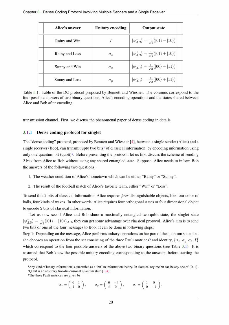
Chapter 3. Dense Coding Protocol Involving Multiple Senders and a Single Receiver

Alice’s answer Unitary encoding Output state

Rainy and Win I | �ABi =

1p2(|01i � |10i)

Rainy and Loss �z | +ABi =

1p2(|01i+ |10i)

Sunny and Win �x |��ABi =

1p2(|00i � |11i)

Sunny and Loss �y |�+ABi =

1p2(|00i+ |11i)

Table 3.1: Table of the DC protocol proposed by Bennett and Wiesner. The columns correspond to thefour possible answers of two binary questions, Alice’s encoding operations and the states shared betweenAlice and Bob after encoding.

transmission channel. First, we discuss the phenomenal paper of dense coding in details.

3.1.1 Dense coding protocol for singlet

The “dense coding” protocol, proposed by Bennett and Wiesner [4], between a single sender (Alice) and asingle receiver (Bob), can transmit upto two bits1 of classical information, by encoding information usingonly one quantum bit (qubit)2. Before presenting the protocol, let us first discuss the scheme of sending2 bits from Alice to Bob without using any shared entangled state. Suppose, Alice needs to inform Bobthe answers of the following two questions:

1. The weather condition of Alice’s hometown which can be either “Rainy” or “Sunny”,

2. The result of the football match of Alice’s favorite team, either “Win” or “Loss”.

To send this 2 bits of classical information, Alice requires four distinguishable objects, like four color ofballs, four kinds of waves. In other words, Alice requires four orthogonal states or four dimensional objectto encode 2 bits of classical information.

Let us now see if Alice and Bob share a maximally entangled two-qubit state, the singlet state| �ABi =

1p2(|01i � |10i)AB , they can get some advantage over classical protocol. Alice’s aim is to send

two bits or one of the four messages to Bob. It can be done in following steps:Step 1: Depending on the message, Alice performs unitary operations on her part of the quantum state, i.e.,she chooses an operation from the set consisting of the three Pauli matrices3 and identity, {�x,�y,�z, I}which correspond to the four possible answers of the above two binary questions (see Table 3.1). It isassumed that Bob knew the possible unitary encoding corresponding to the answers, before starting theprotocol.

1Any kind of binary information is quantified as a “bit” in information theory. In classical regime bit can be any one of {0, 1}.2Qubit is an arbitrary two-dimensional quantum state [174].3The three Pauli matrices are given by

�x =

✓0 11 0

◆, �y =

✓0 �ii 0

◆, �z =

✓1 00 �1

◆.

20

3.1. Dense Coding protocol in a noiseless scenario

Alice’s answer Unitary encoding Output state

Rainy and Win I |�1ABi = a|01i+ b|10i

Rainy and Loss �z |�2ABi = a|01i � b|10i

Sunny and Win �x |�3ABi = a|11i+ b|00i

Sunny and Loss �y |�4ABi = a|11i � b|00i

Table 3.2: Table of the Alice’s unitary encodings and the corresponding output states for a arbitrary sharedbipartite pure quantum state, |�ABi = a|01i+ b|10i.

Step 2. Alice sends her part of the quantum state to Bob, by using a noiseless transmission channel andBob now possess the entire two-qubit state.Step 3. Performing a joint Bell basis measurement, {| ±

i, |�±i}, Bob can identify the message that Alice

has sent to him.In this process, by sending only her part of the quantum state (a single qubit or a two dimensional

object), Alice is able to communicate two bits of classical information to Bob, and hence the capacityof dense coding is considered to be two in this case. Note that, in the entire process, all the answers areconsidered to be equally probable.

Suppose now that Alice and Bob share an arbitrary two-qubit pure quantum state, |�ABi = a|01i +

b|10i, with |a|2 + |b|

2 = 1, instead of a singlet. After performing the same unitary encoding as given inTable 3.2, we note that the encoded states no longer remain mutually orthogonal. Hence Bob will not beable to distinguish the four non-orthogonal states with certainty by using the unitary operations as before4To distinguish them with a non-zero probability, he can perform positive operator valued measurement(POVM) [135], resulting to a probabilistic DC protocol. Protocols unlike the previous deterministic one,we can infer that the capacity decreases when a shared state is nonmaximally entangled which we discuss.We will also discuss how to perform dense coding deterministically with the nonmaximally entangledstate, in the last chapter.

3.1.2 DC for arbitrary shared state

We now consider the dense coding scheme when the sender (Alice) and the receiver (Bob) share anarbitrary quantum state ⇢AB , defined on H

A⌦H

B . Here we assume that both the Hilbert spaces HA andH

B are finite dimensional complex Hilbert spaces, with dimensions dA and dB respectively. Suppose,Alice needs to send Bob some messages {x}, which occur with probabilities px. As discussed in thepreceding section, she applies unitary operator Ux

A, with probability px on her part of the quantum state,

4It is interesting to ask at this point whether there exists other unitary operations which can be performed on non-maximallyentangled states, leading to deterministic transfer of 2 bits. In case of two qubits, it was shown that this is not possible [126].(see also Chapter 7)

21

Chapter 3. Dense Coding Protocol Involving Multiple Senders and a Single Receiver

resulting an ensemble of states E = {px, ⇢xAB}, where

⇢xAB =

�U

xA ⌦ IB

�⇢AB

�U

x†A ⌦ IB

�. (3.1)

Now Alice’s task is to send her part of the ensemble E to Bob by using a noiseless quantum transmissionchannel. Upon receiving the Alice’s part, Bob possess the entire ensemble E = {px, ⇢

xAB}. To gather

maximal information about the message x, Bob has to optimize over a set of measurements {My}. Ifthe measurement outcome turns out to be y, occurring with probability py, then the maximal amount ofinformation that Bob can extract about E , is called the accessible information Iacc, and it is bounded bythe Holevo quantunity [12], given by

Iacc S

⇣X

x

px⇢xAB

⌘�

X

x

pxS�⇢xAB

�

| {z }�(px,⇢xAB

)

. (3.2)

For an arbitrary quantum state shared between Alice and Bob, the maximal amount of information thatAlice is able to send by unitary encoding is called the capacity of dense coding, denoted by C. To obtainthe capacity of DC, one has to perform optimizations over all possible unitary encodings, the probabilitiesof encoding, and over all quantum mechanically allowed measurements performed by the receiver. Theoptimization over measurements for a given set of states is already obtained via the Holevo quantitywhich can be achieved assymptotically [13, 14], i.e., when many copy of the same ensemble is provided.Therefore, the DC capacity, C, reduces to the maximization of the Holevo quantity, over all possibleencodings and probabilities, i.e.,

C(⇢AB) = max{px,Ux

A}�(px, ⇢

xAB). (3.3)

If we focus on the second term of the Holevo quantity in (3.2), we get

X

x

pxS�⇢xAB

�=�X

x

px�S�⇢AB

�= S

�⇢AB

�. (3.4)

This is due to the fact that the unitary operations do not change the spectrum of a density matrix andP

x px = 1. Moreover, if we apply the subadditivity of the von Neumann entropy, the first term in (3.2)reduces to

S

⇣X

x

px⇢xAB

⌘ S

⇣X

x

px⇢xA

⌘+ S

⇣X

x

px⇢xB

⌘

log2 dA + S(⇢B). (3.5)

To obtain the first term in the second line, we use that the von Neumann entropy of ⇢ is bounded aboveby the dimension of the state i.e., S(⇢A) log dA. On the other hand, the second term involves thevon Neumann entropy of the marginal density matrix of Bob, which does not change under the action ofunitary on Alice’s side i.e.,

⇢xB = trA

⇣�U

xA ⌦ IB

�⇢AB

�U

x†A ⌦ IB

�⌘= ⇢B. (3.6)

22

3.1. Dense Coding protocol in a noiseless scenario

Hence the capacity [15–20] in Eq. (3.3) reduces to

C(⇢AB) log2 dA + S(⇢B)� S(⇢AB). (3.7)

It was shown in Ref. [15] that this bound can be achieved by choosing the encoding operations {UxA}

chosen from a complete set of unitary operators {Wx}d2A�1

x=0 2 HA, satisfying the following conditions

1

dAtr(WxW

†y ) = �xy, (3.8)

1

dA

X

x

Wx⌅W†x = tr(⌅)IA, (3.9)

with equal probability px = 1d2A

. Therefore, the DC capacity takes the form

C(⇢AB) = log2 dA + S(⇢B)� S(⇢AB). (3.10)

Note that the first term in Eq. (3.10) is the capacity of classical information transmission withoutsharing of an entangled state, since only d distinct massages can be communicated by transmitting ad dimensional object (classical protocol of information transfer). The negation of quantum conditionalentropy �S(A|B) = S(⇢B) � S(⇢AB) is known as the quantum advantage of the DC protocol [175],or the coherent information [143]. Therefore, positivity of coherent information guarantees the densecodeability of the shared state ⇢AB , which is always the case for a pure entangled states. Note that thequantity S(A|B) becomes sometime positive, which is the situation for all classically correlated (CC)state 5 and hence C(⇢AB) log2 dA, for all CC states. In such a situation, one needs to use the classicalprotocol for information transmission, which always saturates the bound log2 dA. On the other hand, weknow

S(⇢B)� S(⇢AB) S(⇢B) log2 dB, (3.11)

and hence the upper bound on C(⇢AB) is log2 dAB . Therefore, we define the capacity of DC in thefollowing way:

C(⇢AB) =1

log dABmax{log2 dA, log2 dA + S(⇢B)� S(⇢AB)}. (3.12)

If the shared state is a pure one | ABi, then the DC capacity reduces to

C(| ABi) =1

log dABmax{log2 dA, log2 dA + S(⇢B)}, (3.13)

since S(| ABi) = 0. We can compare the DC capacity given in Eq. (3.13), with the protocol describedin Sec 3.1.1. For a shared |

�ABi, the reduced density matrix in the receiver’s subsystem is ⇢B = 1

2I2, andhence C(| �ABi) = log2 2 + 1 = 2, as dA = 2. In d ⌦ d system, the DC capacity reaches its maximumvalue for maximally entangled states, given by

| ABi =1pd

X

i

|iii, (3.14)

5A classically correlated state is ⇢AB =P

ijpij |iAihiA|⌦ |jBihjB |, where {|iAi} and {|jBi} are orthogonal set of states

in the Hilbert spaces of A and B, withP

ijpij = 1.

23

Chapter 3. Dense Coding Protocol Involving Multiple Senders and a Single Receiver

where {|ii} forms a basis in d dimensional Hilbert space. Moreover, from Sec. 2.2.1, we have seen thatfor a pure bipartite state | ABi, E(| ABi) = S(⇢B), and hence we get

C(| ABi) =1

log dABmax{log2 dA, log2 dA + E(| ABi)}. (3.15)

This implies the capacity of classical information transfer for a bipartite shared pure state is directly relatedto the entanglement of the shared state and the state is always useful for DC i� it is not product. We willcome back to this one-to-one connection between the capacity and entanglement in the next chapter formultipartite states which is one of the results presented in this thesis.

3.1.3 Dense coding protocol involving multiple senders and a single receiver

In the multiparty quantum DC protocol, an arbitrary multipartite quantum state, ⇢S1...SNR, is sharedbetween N senders, S1, . . . , SN and a single receiver R. Here we assume that the senders are situated indistant locations. Suppose that the jth sender encodes her messagexj , by performing unitary operatorsUxj

j

on her part of the shared state with probability pxj, and sends it to the only receiver present in the protocol,

with the help of a noiseless quantum channel. Similarly, other senders also perform unitary operations ontheir part, depending on their message. After obtaining the entire ensemble {px, ⇢

xS1...SNR}, where px =

px1px2 . . . pxN, and ⇢xS1...SNR = (Ux1

1 ⌦Ux22 ⌦. . .⌦U

xN

N ⌦IR)⇢S1...SNR(Ux1†1 ⌦U

x2†2 ⌦. . .⌦U

xN †N ⌦IR),

the receiver now performs measurement on the entire state, to gather as much information as possibleabout the message x. In this case also, the information accessible to the receiver is bounded above by theHolevo quantity [12] of the given ensemble

Iacc S

⇣X

x

px⇢xS1...SNR

⌘�

X

x

pxS�⇢xS1...SNR

�. (3.16)

Since it can be achieved in the asymptotic level, the multiparty DC capacity is obtained by performing theoptimization over all unitaries and probabilities i.e.,

C(⇢S1...SNR) = max{pxj },{U

xj

j}

hS

⇣X

x

px⇢xS1...SNR

⌘�

X

x

pxS�⇢xS1...SNR

�i. (3.17)

The optimization has been carried out in Ref. [21] in a similar fashion as discussed in Sec. 3.1.2, and themultiparty DC capacity is given by

C(⇢S1...SNR) = log2 dS1...SN+ S(⇢R)� S(⇢S1...SNR), (3.18)

where dS1...SN= dS1 . . . dSN

, with dSj(j = 1, 2, . . . , N) being the dimensions of the Hilbert spaces of

the individuals sender, Sj and the DC advantage is S(⇢R)� S(⇢S1...SNR) log2 dR, which can be bothpositive and negative, with dR being the dimension of the Hilbert space of the receiver’s subsystem. In mythesis, I will therefore use the multiparty DC capacity of an arbitrary N + 1 party shared state ⇢S1...SNR,as

Cmulti(⇢S1...SNR) =

1

log dS1...SNRmax{log dS1...SN

, log dS1...SN+ S(⇢R)� S(⇢S1...SNR)}. (3.19)

The state will be useful for multiparty DC if S(⇢R)� S(⇢S1...SNR) > 0.

24

3.2. Dense coding capacity in presence of noise

3.2 Dense coding capacity in presence of noise

In this section, we discuss the capacity of classical information transfer in presence of noise. In particular,since the system can not be kept completely isolated from the environment, the noise is unavoidable and isinevitably present in the system [125,135]. Noise can in general decrease the quantum correlation presentin the system and hence decreases its ability in performing many quantum technological tasks, includingquantum communicational capacity.

The noise in a quantum channel of the DC protocol can be considered at several levels of complexity.We consider mainly following two scenarios:

1. We consider the case where the noise is present before the encoding of classical information, i.e.,noise interacts in the quantum system when it is shared between the senders and the receiver. Inthis case, we assume that the quantum channel that transmits the encoded state is noiseless.

2. We consider another situation where after the encoding is performed on the sender’s part of theshared state, noise acts at the time of sending the encoded part of the senders through a quantumchannel. It includes the previous situation as well.

Before presenting the e�ects of noise on the capacity of DC, let us discuss di�erent types of noise andtheir formalism that we will use in my thesis.

3.2.1 Mathematical description of noise

Mathematically, noise can be described [125,135] as a completely positive trace preserving (CPTP) map,⇤ and a quantum state ⇢ after passing through a noisy channel, ⇤ transforms as

⇢ :! ⇤(⇢), (3.20)

with the following properties

1. Linearity: ⇤(↵⇢1 + �⇢2) = ↵⇤(⇢1) + ��(⇢2).

2. Hermiticity: ⇢ = ⇢†) ⇤(⇢) = ⇤(⇢†).

3. Trace preserving: tr(⇢) = tr�⇤(⇢)

�= 1, 8⇢.

4. Positive: ⇤(⇢) � 0, 8 ⇢ � 0.

5. Completely positive: For a bipartite state⇢AB , if noise⇤A acts only on the subsystemA,⇤A(⇢AB) �

0, 8 ⇢AB .

The last property is not true for all maps, which are satisfying the properties 1. � 4. For example,one can consider the partial transposition (PT ) map [99], which acts on a composite state ⇢AB , asPT (⇢AB) = ⇢

TA

AB , (see Eq. (2.19)), resulting an operator which is not always positive as shown inRefs. [96–100]. Hence PT map is positive but not completely positive.

The noise model can be considered as an interaction of the system ⇢S with the environment, which weconsider to be in a state |0iE . Now the joint state is ⇢S ⌦ |0ih0|E , and any quantum interaction between

25

Chapter 3. Dense Coding Protocol Involving Multiple Senders and a Single Receiver

the system S and the environment E, can be described by a joint unitary operator USE , acting on theentire system-environment duo. Therefore, the system transforms as

⇤(⇢S) = trE�USE(⇢S ⌦ |0ih0|E)U

†SE

�

=X

↵

Eh↵|USE(⇢S ⌦ |0ih0|E)U†SE |↵iE

=X

↵

Eh↵|USE |0iE⇢Sh0|U†SE |↵iE

=X

↵

K↵⇢SK†↵, (3.21)

where {|↵iE} is a set of orthogonal basis in the Hilbert space of the environment andK↵ = Eh↵|USE |0iE .Therefore, the noise model, i.e., the linear map ⇤, can be expressed as the operator sum representation[176] given in Eq. (3.21) by using operators {K↵}, known as Kraus operators [125, 135, 176], withP

↵K†↵K↵ = I, belonging to the same Hilbert space in which the quantum state systems ⇢ is defined and

over which it acts and ⇤ is called quantum channels, represented by

⇤(⇢) =X

↵

K↵⇢K†↵. (3.22)

3.2.2 Examples of noisy quantum channels

In the realm of quantum information and computation, the noise can either interact with the entire systemor some parts of the system or locally in each parts of the system. The noise model can be divided intotwo broad categories. For an N-party quantum state, ⇢1...N , they are

1. global noise, and

2. local noise.

Global noise

A noise model, ⇤G, acting on a system of N parties, ⇢1...N , is said to be global if it acts as

⇤G(⇢1...N ) =X

↵

K↵⇢1...NK†↵, (3.23)

where {K↵}, is the set of Kraus operator defined in the joint Hilbert space of all the parties, satisfyingP

↵K†↵K↵ = I1...N . If the action of the {Kj

↵}Nj=1 on each subsystem reads as

⇤G(⇢1...N ) =X

↵

K1↵ ⌦ . . .⌦ K

N↵ ⇢1...NK

1†↵ ⌦ . . .⌦ K

N†↵ , (3.24)

the noise can be called completely correlated noise model and can also be considered as a global noisemodel. If {Kj

↵}Nj=1 are chosen from the Pauli matrices, it is then known as fully correlated Pauli channel,

as will be discussed later.

26

3.2. Dense coding capacity in presence of noise

Local Noise

In contrast to the global noise, the local noise acts locally on the subsystems of the entire state, ⇢1...N , as

⇤L(⇢1...N ) =X

{↵}

KA1↵1⌦ . . .⌦K

Ar

↵r⇢1...NK

A1†↵1⌦ . . .⌦K

Ar†↵r

, (3.25)

where A1 [ A2 . . . [ Ar = N , and A1 \ A2 . . . \ Ar = ;, with ; being the null set and KAj

↵jis some

Kraus operator in the Hilbert space of the system Aj , which can comprise of few subsystems of the entiresystem or a single system. It is called completely uncorrelated or completely local if

⇤L(⇢1...N ) =X

{↵}

K1↵1⌦ . . .⌦K

N↵N⇢1...NK

1†↵1⌦ . . .⌦K

N†↵N

, (3.26)

where Kj↵j

represents the Kraus operator on the jth system which is a subclass of the model, given in Eq.(3.25).

For the qubit system, there are many examples of noisy channels [125,135], for which Kraus operatorscan be found. The examples of channels that we will use in this thesis are

(a) amplitude damping channel.

(b) phase damping channel.

(c) Pauli channel.

These channels play important roles in the problem of decoherence [125]. The amplitude damping channelhas been used to model the spontaneous decay of a photon from an excited atomic state to its ground state,while the phase damping one can correspond to scattering events. Pauli channels include a reasonablylarge class of quantum channels like the bit flip, and depolarizing channels, and also play an important rolein the problem of decoherence. Pauli channels have been used to study the Pauli cloning machine [177],and they comprise a huge class of noisy channels. We will now discuss them individually and will writedown the Kraus operators.

Amplitude damping channel

A single qubit ⇢, after passing through the amplitude damping channel, transforms as

⇢ �! ⇤AD� (⇢) = M0⇢M

†0 +M1⇢M

†1 , (3.27)

where the Kraus operators, Mi (i = 0, 1), are given by

M0 =

1 0

0p1� �

!, M1 =

0p�

0 0

!, (3.28)

satisfying the conditionM

†0M0 +M

†1M1 = 1, (3.29)

with 0 � 1 being the noise parameter.

27

Chapter 3. Dense Coding Protocol Involving Multiple Senders and a Single Receiver

Phase damping channel

Phase damping channel or dephasing channel, ⇤PD, acts on a single qubit state ⇢, in the following way:

⇤PD(⇢) = M0⇢M†0 +M1⇢M

†1 +M2⇢M

†2 , (3.30)

where the Mi’s are

M0 =

p1� p 0

0p1� p

!, M1 =

pp 0

0 0

!, M2 =

0 0

0pp

!, (3.31)

with 0 p 1 being the noise parameter.

Pauli channel

In case of Pauli channel, the Kraus operators are chosen from the Pauli matrices, given by

�x =

0 1

1 0

!, �y =

0 �i

i 0

!, �z =

1 0

0 �1

!. (3.32)

When an arbitrary qubit state, ⇢, is passed through the Pauli channel [59, 178, 179], the resulting state isgiven by

⇤P (⇢) =3X

m=0

qm�m⇢�

m (3.33)

where �1 = �x, �2 = �y, �3 = �z and �0 =

1 0

0 1

!is the identity operator in the Hilbert space of

two dimension. Here {qm}3m=0, are the probability in which di�erent Pauli matrices are acting on the

system andP

m qm = 1. Depending on the probabilities, the Pauli channel can be divided into severalsubcategories [125, 135]. Here we list some of them which we will use later in the thesis.

(i) Bit flip channel: q2 = q3 = 0.

(ii) Phase flip channel: q1 = q2 = 0.

(iii) Bit phase flip channel: q1 = q3 = 0.

(iv) Depolarizing channel: q1 = q2 = q3 =q3 , where 0 q 1.

For a two-qubit quantum state ⇢AB , if both the parties are going through Pauli channels, the outputstate reads as

⇤P (⇢AB) =3X

mn=0

qmn�m⌦ �

n⇢AB�

m⌦ �

n, (3.34)

where {qmn} is the set of probability by which the Pauli matrices are acting on the system. Two di�erentkinds of noise models emerge from Eq. (3.34), which are given below.Case 1: Fully correlated Pauli channel with qmn = qm�mn, or a global Pauli channel:

⇤Pc (⇢AB) =

3X

m=0

qm�m⌦ �

m⇢AB�

m⌦ �

m, (3.35)

28

3.2. Dense coding capacity in presence of noise

Case 2: Completely uncorrelated Pauli channel with qmn = qmqn, or local Pauli channel:

⇤Puc(⇢AB) =

3X

mn=0

qmqn�m⌦ �

n⇢AB�

m⌦ �

n, (3.36)

These two channels can also be extended to higher number of parties like in Eq. (3.26).

3.2.3 Capacity of DC for covariant noise

As we have already mentioned, there are two ways in which capacity of DC can be a�ected under noise.In the first case, the shared quantum state ⇢ gets a�ected by the noise model ⇤ at the time of sharing ofthe state between all the senders and the receiver. As a result, ⇢! ⇤(⇢), and since the output state is alsoa valid quantum state, one can use Eq. (3.19) to obtain C(⇤(⇢)), which is valid for arbitrary multipartyquantum state. It is clear from Eq. (3.22), that any pure state, | i, is likely to transform into a mixed state,under noisy channel and hence the DC capacity for pure states under noisy environment decreases withnoise parameter.

In the second situation, we consider that the noise, ⇤, acts only on the senders’ part of the encodedstate, at the time of sending it to the receiver. Hence, the ensemble that the senders are intended to transfer,is distorted like

{px, ⇢xS1...SNR}! {px,⇤(⇢

xS1...SNR)}, (3.37)

where⇤(⇢xS1...SNR) =

X

µ

�Kµ ⌦ IR

�⇢xS1...SNR

�K

†µ ⌦ IR

�, (3.38)

with {Kµ} being the set of Kraus operators in the Hilbert space of all the senders. It surely results decreaseof accessible information that the receiver is supposed to get from the senders. Note that this situation iscompletely di�erent from the previous one, and one can not apply Eq. (3.19) in this case6. However, theHolevo quantity is still valid and the amount of information that the receiver can extract is again boundedby [12]

Inoiseacc S

⇣X

x

px⇤�⇢xS1...SNR

�⌘�

X

x

pxS

⇣⇤�⇢xS1...SNR

�⌘, (3.39)

which can be achieved asymptotically, in this situation also [13, 14]. Therefore, the noisy DC capacity isdefined as

Cn(⇢S1...SNR) = max{pxj },{U

xj

j}

hS

⇣X

x

px⇤�⇢xS1...SNR

�⌘�

X

x

pxS

⇣⇤�⇢xS1...SNR

�⌘i. (3.40)

For any arbitrary noise model, finding the optimized unitary encodings and the probabilities is complicatedand is still an open question. But for a certain class of noise model like the “covariant noise” [59], theoptimization has been carried out and the noisy capacity of DC is obtained in Refs. [23–26]. The covariantnoise, ⇤c, is a CPTP map which commutes with a particular set of orthogonal unitaries {Wi}, satisfying

6 It also includes the previous situation. Since ⇢S1...SNR can be generated from noisy initial state.

29

Chapter 3. Dense Coding Protocol Involving Multiple Senders and a Single Receiver

the properties listed in Eqs. (3.8) and (3.9), and is given by

⇤C(Wi⇢W†i ) = Wi⇤

c(⇢)W †i , 8i. (3.41)

For example, the Pauli channel, introduced in Eq. (3.33) of Sec. 3.2.2, is a covariant channel whichcommutes with a particular set of orthogonal unitary operators, the Pauli spin matrices itself [59,178,179].If we assume that the noise is present only in the transmission channel, through which the senders sendtheir encoded part to the receiver, ⇤c then acts only on the senders system, and as it is a CPTP map,the output state is also a valid quantum state. Moreover, the marginal density matrix in the receiver’ssubsystem, ⇢R, remains unperturbed.

Therefore, the capacity of DC under covariant channel reads as

Cn(⇢S1...SNR) = log2 dS1...SN+ S(⇢R)� S(⇢), (3.42)

where⇢ = ⇤c

⇣(Umin

S1S2...SN⌦ IR)⇢S1...SNR(U

min†S1S2...SN

⌦ IR)⌘.

Here, UminS1S2...SN

denotes the unitary operator on the senders’ side, which minimizes the von Neumannentropy of (US1...SN

⌦ IR)⇢S1...SNR(U†S1...SN

⌦ IR) over the set of unitaries {US1S2...SN}, that can be

global as well as local, depending on the type of encoding. It is reasonable from a practical point of viewto assume that the senders perform local encoding. Then U

minS1S2...SN

takes the form given by

UminS1S2...SN

= UminS1⌦ U

minS2⌦ ...⌦ U

minSN

. (3.43)

Like in the previous cases, the upper bound of Cn is log2 dS1...SNR, and the classical limit is log2 dS1...SN.

Finally, the noisy DC capacity for N senders and a single receiver is given by

Cnoisy(⇢S1...SNR) =

1

log2 dS1...SNRmax{log2 dS1...SN

, log2 dS1...SN+ S(⇢R)� S(⇢)}. (3.44)

Depending on the structure of ⇤c, the channel can be either correlated (global) or uncorrelated (local), asdefined earlier.

30

Chapter 4Multipartite Dense Coding vs. QuantumCorrelations

In the realm of quantum information and computation, it was a well-established fact both theoretically aswell as experimentally, that bipartite entanglement is an essential ingredient for a vast majority of knownquantum communication schemes, involving two parties [2–8]. Specifically, it has been established thatin case of pure bipartite states, | ABi, the capacity of classical information transmission by a sharedquantum state (for dense coding capacity see Eq. (3.13)) increases with the increase (see Eq. (3.15))of quantum correlations quantified according to any measure (see Sec. 2.2.1). Unlike point-to-pointcommunication, involving two parties, a sender and a receiver, communication protocols with multipleparties can have various complexities. One possible scenario involves several senders and a singlereceiver, and in this chapter we will restrict ourselves to this situation only. Suitable examples of suchmultipartite communication protocols include several news reporters from di�erent locations, sendingvarious news articles to the editorial o�ce of the newspaper or several weather observers from di�erentplaces communicating their respective weather reports to the regional meteorological o�ce.

In this chapter, our main goal is to connect multipartite communication protocols with multipartyquantum correlation measures. In particular, we establish a relation between the capacity of multipartiteDC and multipartite quantum correlation measures of arbitrary multiqubit states. Such a relation existsfor bipartite states and is particularly simple for bipartite pure states. Applications of quantum channelsare most likely to be commercially important only in the multiparty domain. However, very little isknown about the qualitative structure and the exact values of capacities of multiparty quantum channelsexcept the case with multiple senders and a single or two receivers. In recent times, a lot of interests hasbeen created to characterize and quantify quantum communication schemes in multiparty regime [21,22].But a sheer connection between the DC capacity in the multiparty domain and the multiparty quantumcorrelation measures is still missing. This may be due to the fact that there is no unique measure ofmultiparty quantum correlation even for multiparty pure states, as derived in Eq. (3.13). In this chapter,we will establish relations between multiparty DC capacity with a single receiver and multiparty quantumcorrelation measures defined from two di�erent paradigms. The correspondence that we establish isillustrated in the cases of both noiseless and noisy channels for arbitrary shared states.

31

Chapter 4. Multipartite Dense Coding vs. Quantum Correlations

4.1 Connection of QC measures with capacity DC in a noiseless scenario

In this section, we establish a generic relation between the multiparty DC capacity and various multipartyQC measures, defined in Chapter. 2. The multiparty measures with which we establish the connectionsare the genuine multiparty entanglement measure [28, 29], defined in Sec. 2.4.1, the monogamy basedmeasures the tangle and discord monogamy score (see Sec. 2.4.2). Throughout this section, we considerthe case when the additional quantum channel, that is used post-encoding, is noiseless.

4.1.1 Connection with genuine multiparty entanglement measure

In a bipartite scenario, all the pure states having same amount of entanglement have equal capacity ofdense coding. The entanglement in this case is uniquely quantified by the von Neumann entropy of thelocal density matrices and the capacity is maximal for the maximally entangled states [4].

We will see that this simple situation is no more true in the multiparty regime. However, it is stillpossible to obtain a generic relation between capacity and entanglement. In a multipartite scenario, quan-tification of quantum correlations is not unique even for pure states and hence each measure, in principle,identifies its own distinct state with maximal quantum correlation. Nevertheless, the Greenberger-Horne-Zeilinger (GHZ) state [56] has been found to possess a high amount of multipartite quantum correlation,according to violation of certain Bell inequalities [180–182], as well as according to several multipartiteentanglement measures [27–29]. In view of these results, we compare the properties of an arbitrary(N + 1)-qubit1 pure state with that of the (N + 1)-qubit generalized GHZ state (gGHZ), which is givenby

|gGHZiS1S2...SNR =p↵|0S1 . . . 0SN

i|0Ri+p1� ↵ei�|1S1 . . . 1SN

i|1Ri, (4.1)

where ↵ is the real number in (0, 1)2 and � 2 [0, 2⇡). We find that if the capacity of dense coding withN senders and a single receivers, of an arbitrary (N +1)-party state, | iN+1, and the gGHZ state are thesame, then the genuine multiparty entanglement measure in terms of the generalized geometric measure(GGM), defined in (Eq. (2.39), of these two states may not be the same. However, they follow an ordering,which we establish in the following theorem. Here on, we skip all the subscripts in the notation of thestates, for simplicity.Theorem 1: Of all the multiqubit pure states with an arbitrary but fixed multiparty dense coding capacity,the generalized GHZ state has the highest GGM.Proof. Scanning over ↵ in Eq. (4.1), one can obtain an arbitrary value of the GGM. Therefore, to provethe theorem, one needs to show that if the multiparty dense coding capacity of an arbitrary (N +1)-qubitpure state is the same as that of an (N +1)-party gGHZ state, then the genuine multipartite entanglement,as quantified by the GGM, of that arbitrary pure state is bounded above by that of the gGHZ state, i.e.,

E(| i) E(|gGHZi), (4.2)

providedC

multi(| i) = Cmulti(|gGHZi). (4.3)

1(N + 1)-qubit system comprises tensor product Hilbert spaces of (N + 1) two level systems of dimension 2N+1.2 We exclude two points, ↵ = 0 and ↵ = 1, from the definition of gGHZ state as in those points the states no longer remain

an entangled state and they are |1S1 . . . 1SN i|1Ri and |0S1 . . . 0SN i|0Ri respectively.

32

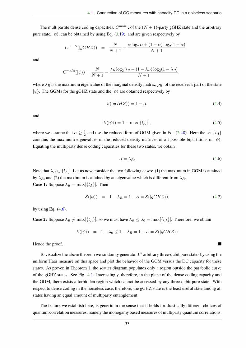
4.1. Connection of QC measures with capacity DC in a noiseless scenario

The multipartite dense coding capacities, Cmulti, of the (N + 1)-party gGHZ state and the arbitrarypure state, | i, can be obtained by using Eq. (3.19), and are given respectively by

Cmulti(|gGHZi) =

N

N + 1�↵ log2 ↵+ (1� ↵) log2(1� ↵)

N + 1

and

Cmulti(| i) =

N

N + 1��R log2 �R + (1� �R) log2(1� �R)

N + 1,

where �R is the maximum eigenvalue of the marginal density matrix, ⇢R, of the receiver’s part of the state| i. The GGMs for the gGHZ state and the | i are obtained respectively by

E(|gGHZi) = 1� ↵, (4.4)

andE(| i) = 1�max[{lA}], (4.5)

where we assume that ↵ � 12 and use the reduced form of GGM given in Eq. (2.48). Here the set {lA}

contains the maximum eigenvalues of the reduced density matrices of all possible bipartitions of | i.Equating the multiparty dense coding capacities for these two states, we obtain

↵ = �R. (4.6)

Note that �R 2 {lA}. Let us now consider the two following cases: (1) the maximum in GGM is attainedby �R, and (2) the maximum is attained by an eigenvalue which is di�erent from �R.Case 1: Suppose �R = max[{lA}]. Then

E(| i) = 1� �R = 1� ↵ = E(|gGHZi), (4.7)

by using Eq. (4.6).

Case 2: Suppose �R 6= max[{lA}], so we must have �R �0 = max[{lA}]. Therefore, we obtain

E(| i) = 1� �0 1� �R = 1� ↵ = E(|gGHZi)

Hence the proof. ⌅

To visualize the above theorem we randomly generate 105 arbitrary three-qubit pure states by using theuniform Haar measure on this space and plot the behavior of the GGM versus the DC capacity for thesestates. As proven in Theorem 1, the scatter diagram populates only a region outside the parabolic curveof the gGHZ states. See Fig. 4.1. Interestingly, therefore, in the plane of the dense coding capacity andthe GGM, there exists a forbidden region which cannot be accessed by any three-qubit pure state. Withrespect to dense coding in the noiseless case, therefore, the gGHZ state is the least useful state among allstates having an equal amount of multiparty entanglement.

The feature we establish here, is generic in the sense that it holds for drastically di�erent choices ofquantum correlation measures, namely the monogamy based measures of multiparty quantum correlations.

33

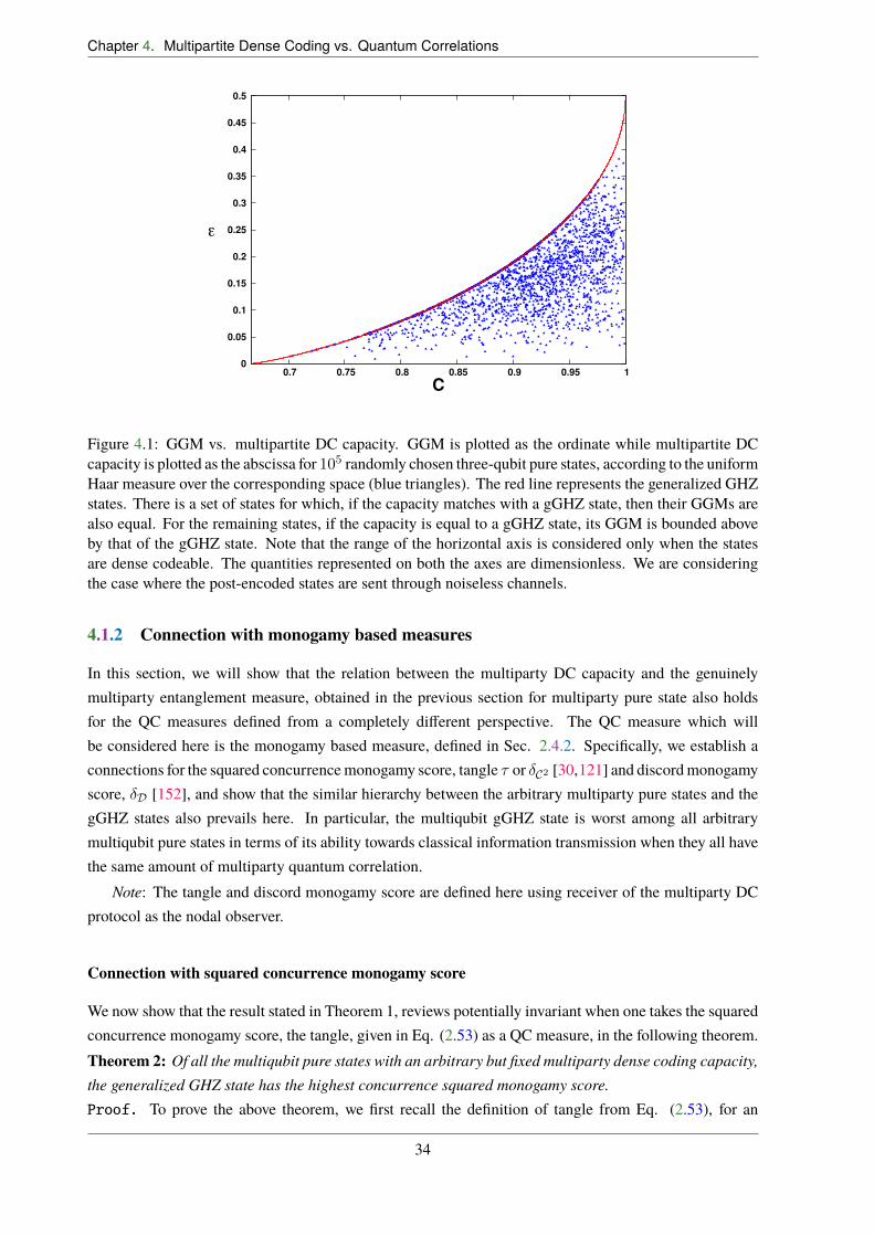
Chapter 4. Multipartite Dense Coding vs. Quantum Correlations

0

0.05

0.1

0.15

0.2

0.25

0.3

0.35

0.4

0.45

0.5

0.7 0.75 0.8 0.85 0.9 0.95 1

ε

C

Figure 4.1: GGM vs. multipartite DC capacity. GGM is plotted as the ordinate while multipartite DCcapacity is plotted as the abscissa for 105 randomly chosen three-qubit pure states, according to the uniformHaar measure over the corresponding space (blue triangles). The red line represents the generalized GHZstates. There is a set of states for which, if the capacity matches with a gGHZ state, then their GGMs arealso equal. For the remaining states, if the capacity is equal to a gGHZ state, its GGM is bounded aboveby that of the gGHZ state. Note that the range of the horizontal axis is considered only when the statesare dense codeable. The quantities represented on both the axes are dimensionless. We are consideringthe case where the post-encoded states are sent through noiseless channels.

4.1.2 Connection with monogamy based measures

In this section, we will show that the relation between the multiparty DC capacity and the genuinelymultiparty entanglement measure, obtained in the previous section for multiparty pure state also holdsfor the QC measures defined from a completely di�erent perspective. The QC measure which willbe considered here is the monogamy based measure, defined in Sec. 2.4.2. Specifically, we establish aconnections for the squared concurrence monogamy score, tangle ⌧ or �C2 [30,121] and discord monogamyscore, �D [152], and show that the similar hierarchy between the arbitrary multiparty pure states and thegGHZ states also prevails here. In particular, the multiqubit gGHZ state is worst among all arbitrarymultiqubit pure states in terms of its ability towards classical information transmission when they all havethe same amount of multiparty quantum correlation.

Note: The tangle and discord monogamy score are defined here using receiver of the multiparty DCprotocol as the nodal observer.

Connection with squared concurrence monogamy score

We now show that the result stated in Theorem 1, reviews potentially invariant when one takes the squaredconcurrence monogamy score, the tangle, given in Eq. (2.53) as a QC measure, in the following theorem.Theorem 2: Of all the multiqubit pure states with an arbitrary but fixed multiparty dense coding capacity,the generalized GHZ state has the highest concurrence squared monogamy score.Proof. To prove the above theorem, we first recall the definition of tangle from Eq. (2.53), for an

34

4.1. Connection of QC measures with capacity DC in a noiseless scenario

(N + 1)-qubit pure state | i, with the receiver as a nodal observer.

⌧(| i) = C2S1...SN :R(| i)�

X

i

C2(⇢SiR), (4.8)

where ⇢SiR is the reduced density matrix of the ith sender and the receiver. The first term in the aboveequation quantifies the squared concurrence of the pure state | i, in the bipartition of all the senders andthe receiver, and it is given by

C2S1...SN :R(| i) = 4 det(⇢R) = 4�R(1� �R), (4.9)

where we use the form of concurrence for the pure state given in Eq. (2.17). Now the tangle for the gGHZstate given in Eq. (4.1) is

⌧(|gGHZi) = 4↵(1� ↵), (4.10)

since all the reduced density matrices of the gGHZ state,

⇢gGHZSiR

=�↵|00ih00|+ (1� ↵)|11ih11|

�SiR

, (4.11)

are separable, and hence C(⇢gGHZSiR

) = 0. Now, the equality of the multipartite DC capacities of these twostates provide ↵ = �R �

12 . Therefore, we have

⌧(| i) = 4 det(⇢R)�X

i

C2(⇢SiR) (4.12)

4�R(1� �R) = 4↵(1� ↵) = ⌧(|gGHZi). (4.13)

Hence proved. ⌅

Connection with discord monogamy score

We also have a similar relation between the multiparty DC capacity with N senders and a single receiverand discord monogamy score for the qubit system as stated in the followingTheorem 3: Of all the multiqubit pure states with an arbitrary but fixed multiparty dense coding capacity,the generalized GHZ state has the highest discord monogamy score.Proof. For an (N + 1)-qubit arbitrary | i, the discord monogamy score is given by

�D(| i) = S(⇢R)�X

i

D(⇢SiR) (4.14)

S(⇢R) = h(�R) = h(↵) = �D(|gGHZi), (4.15)

where S(⇢R) is the von-Neumann entropy (see Eq. (2.6)) of the reduced density matrix in the receiverssubsystem and h(x) is the binary Shannon entropy as given in Eq. (2.14). Here we use the facts thatdiscord is a non-negative quantity, which reduces to S(⇢R) for a multiparty pure state in the senders :receiver bipartition, and

�D(|gGHZi) = h(↵), (4.16)

35

Chapter 4. Multipartite Dense Coding vs. Quantum Correlations

0

0.25

0.5

0.75

1

0.7 0.8 0.9 1

δC

2

C

-0.25

0

0.25

0.5

0.75

1

0.7 0.8 0.9 1

δD

C

Figure 4.2: Left: Tangle (vertical axis) vs. multiparty DC capacity (horizontal axis) for randomlygenerated three-qubit pure states (blue triangles). Right: Discord monogamy score (vertical axis) vs. DCcapacity (horizontal axis) for the same states. In both the cases, the gGHZ states give the boundary (redline). The capacity is dimensionless, while the tangle and discord monogamy score are measured in ebitsand bits, respectively. All other considerations are the same as in Fig. 4.1.

since D(⇢gGHZSiR

) = 0.3 due to the separable states as in Eq. (4.11). Hence the proof. ⌅Note that Theorem 3 holds irrespective of the party on which the measurement is performed for the

evaluation of quantum discord according to Eq. (2.33).To visualize the above theorems, we again randomly generate 105 pure three-qubit states, by using

the uniform Haar measure in the corresponding space, and prepare scatter diagrams for tangle versus themultiparty DC capacity (Fig. 4.2 (left)) and for the discord monogamy score against the same capacity(Fig. 4.2 (right)). The simulations are clearly in agreement with Theorem 2 and 3. In particular, andjust like for GGM with the DC capacity, the planes of (C, �C2) and (C, �D) can not be fully accessedby the three-qubit pure states. The discords in Fig. 4.2 (right), have been calculated by performing themeasurement in the nodal party R. However, note that measurements in the first party also leads to thesimilar results.

4.2 Multiparty DC vs. QC for multiparty mixed state

We now investigate the relation between DC capacity and multipartite quantum correlation measures,when the shared quantum state is an arbitrary (N + 1)-party mixed state. This relation can be consideredas a connection of QC with one kind noisy DC capacity, where the noise is acting on the quantumstate at the time of sharing it among all the senders and the receiver. In this case, to establish suchconnection, the main di�culty is that there are only a few quantum correlation measures available whichcan be computed. Therefore, we consider the discord monogamy score as the multipartite quantumcorrelation measure, since quantum discord can be numerically calculated for arbitrary bipartite systems,and investigate its connection with the DC capacity.

In Fig. 4.3, we randomly generate 105 mixed states of rank-2 in the space of three-qubit statesand plot the discord monogamy score with respect to the DC capacity. The random generation is withrespect to the uniform Haar measure induced from that in the appropriate higher-dimensional pure state

3The reduced density matrix of the gGHZ state, given in Eq. (4.1), is an example of a classically correlated state, defined inEq. (2.38)

36

4.2. Multiparty DC vs. QC for multiparty mixed state

space. The numerical simulation reveals that Theorem 2 does not hold for rank-2 (mixed) three-qubitstates. In particular, we find that if a gGHZ state and a rank-2 three-qubit mixed state have the samediscord monogamy score, then sharing the gGHZ state is usually more beneficial than the mixed state, forperforming the multiparty DC protocol. More precisely, among randomly generated 105 rank-2 states,there are only 1.85% states which satisfy Theorem 2. We will later show that a similar picture is true whenone considers noise in the transmission channel of the DC protocol. This implies that in the presence ofnoisy environments, irrespective of whether the noise is a�icted before or after encoding, it is typicallybetter to share a gGHZ state among states with a given discord monogamy score, from the perspective ofDC capacity. Before presenting the results obtained by using numerical simulations for higher-rank mixedstates, let us discuss the behavior of the DC capacity, as enunciated in the following proposition. Wewill find that it can be used to intuitively understand the numerical results for higher-rank states presentedbelow.

Proposition 1: An arbitrary (N + 1)-qubit (pure or mixed) state is dense codeable if the maximumeigenvalue of the (N + 1)-party state is strictly greater than the maximum eigenvalue of its reduced stateat the receiver’s side.

Proof: An (N + 1)-qubit (pure or mixed) state, ⇢S1S2...SNR, is multiparty dense codeable with N

senders, S1, S2, . . . , SN , and a single receiver, R, if and only if the von Neumann entropy of the reducedstate at the receiver’s side is greater than that of the state ⇢S1S2...SNR, i.e.,

S(⇢R) > S(⇢S1S2...SNR). (4.17)

Let the eigenvalues, in descending order, of the state ⇢R, be given by �R = {�1�

12 , 1 � �

1}. Let

the eigenvalues of the state ⇢S1S2...SNR be �S1S2...SNR = {µi}ri=1, where r is the rank of the matrix,

and where the µi’s are arranged in descending order. Specifically, µ1 gives the largest eigenvalue of

⇢S1S2...SNR. Now, the ordering between the highest eigenvalues of ⇢R and ⇢S1S2...SNR, i.e., between �1

and µ1, can have three possibilities, i.e., �1 > µ

1, or they are equal, or �1 < µ1.

Let us assume that �1 � µ1. Then, invoking the condition of majorization [183], we have

�R � �S1S2...SNR,

which impliesS(⇢R) S(⇢S1S2...SNR). (4.18)

It immediately implies that the state is not dense codeable. Therefore, to obtain dense codeability of⇢S1S2...SNR, we must have �1 < µ

1.Hence the proof. ⌅

Although the above proposition has been presented for qubit systems, it is also valid for an arbitrary(pure or mixed) (N + 1)-party quantum state in arbitrary dimensions, provided ⇢R is of rank 2.

Let us now move to mixed states with higher-rank. Numerically, to obtain high-rank three-qubitmixed states, one possibility is to generate pure states with more than three parties. For example, to obtainarbitrary rank-4 states of three qubits, 5-qubit pure states can be created randomly, and then two partiestraced out. However, numerical searches become ine�cient with the increase of number of parties [184].

37

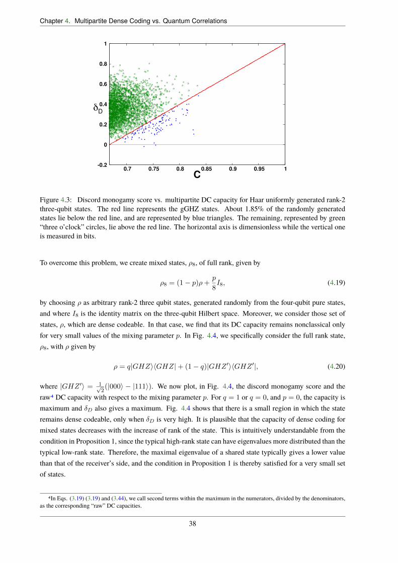
Chapter 4. Multipartite Dense Coding vs. Quantum Correlations

-0.2

0

0.2

0.4

0.6

0.8

1

0.7 0.75 0.8 0.85 0.9 0.95 1

δD

C

Figure 4.3: Discord monogamy score vs. multipartite DC capacity for Haar uniformly generated rank-2three-qubit states. The red line represents the gGHZ states. About 1.85% of the randomly generatedstates lie below the red line, and are represented by blue triangles. The remaining, represented by green“three o’clock” circles, lie above the red line. The horizontal axis is dimensionless while the vertical oneis measured in bits.

To overcome this problem, we create mixed states, ⇢8, of full rank, given by

⇢8 = (1� p)⇢+p

8I8, (4.19)

by choosing ⇢ as arbitrary rank-2 three qubit states, generated randomly from the four-qubit pure states,and where I8 is the identity matrix on the three-qubit Hilbert space. Moreover, we consider those set ofstates, ⇢, which are dense codeable. In that case, we find that its DC capacity remains nonclassical onlyfor very small values of the mixing parameter p. In Fig. 4.4, we specifically consider the full rank state,⇢8, with ⇢ given by

⇢ = q|GHZihGHZ|+ (1� q)|GHZ0ihGHZ

0|, (4.20)

where |GHZ0i = 1p

2(|000i � |111i). We now plot, in Fig. 4.4, the discord monogamy score and the

raw4 DC capacity with respect to the mixing parameter p. For q = 1 or q = 0, and p = 0, the capacity ismaximum and �D also gives a maximum. Fig. 4.4 shows that there is a small region in which the stateremains dense codeable, only when �D is very high. It is plausible that the capacity of dense coding formixed states decreases with the increase of rank of the state. This is intuitively understandable from thecondition in Proposition 1, since the typical high-rank state can have eigenvalues more distributed than thetypical low-rank state. Therefore, the maximal eigenvalue of a shared state typically gives a lower valuethan that of the receiver’s side, and the condition in Proposition 1 is thereby satisfied for a very small setof states.

4In Eqs. (3.19) (3.19) and (3.44), we call second terms within the maximum in the numerators, divided by the denominators,as the corresponding “raw” DC capacities.

38

4.3. Relation of multiparty QC measures with capacity of DC in presence of noise

0 0.2 0.4 0.6 0.8 1 0 0.2

0.4 0.6

0.8 1

0

0.2

0.4

0.6

0.8

1

δD

q = 0.0q = 0.04q = 0.08q = 0.12q = 0.16q = 0.20q = 0.24

C

p

δD

Figure 4.4: Discord monogamy score and the raw DC capacity are plotted against the mixing parameterp, for the rank-8 state, ⇢8 = (1� p)⇢+ p

8I . Here ⇢ = q|GHZihGHZ|+ (1� q)|GHZ0ihGHZ

0|. Each

value of q provides a curve, and we present several exemplary curves in the figure. All the quantitiesplotted are dimensionless, except �D, which is measured in bits.

4.3 Relation of multiparty QC measures with capacity of DC in presenceof noise

In this section, we establish a connection between the multiparty QC measures and the DC capacity ofnoisy channels, for both correlated and uncorrelated noise, for the (N+1)-party state, ⇢S1S2...SNR, sharedbetween N senders and a single receiver. Here we assume that the N senders individually apply localunitary operations on their parts of the shared state and send their encoded parts through a covariantnoisy channel (see Sec. 3.2.3). As the encoding has been carried out over the quantum state upon whichno noise is acted, so we use here the QC measures of the initial states. We now address the extent towhich the relation, established in Sec. 4.1, between multiparty DC capacity for the noiseless channeland multipartite QC measures, in the case of pure shared quantum states, still remains valid for the noisychannel scenario. To this end, we consider two extreme scenarios, one in which the noise between thedi�erent sender qubits are fully correlated, and another in which the same are uncorrelated.

4.3.1 Fully correlated Pauli channel

An (N + 1)-qubit state, ⇢S1S2...SNR, after being acted on by the fully correlated Pauli channel, presentedin Eq. (3.35), is given by

⇤P (⇢S1S2...SNR) =3X

i=0

qm(�mS1⌦ · · ·⌦ �

mSN⌦ IR)⇢S1S2...SNR(�

mS1⌦ · · ·⌦ �

mSN⌦ IR), (4.21)

whereP3

m=0 qm = 1, and qm � 0, and where we denote, for simplicity, �x = �1,�y = �

2,�z = �

3, and

the identity matrix as �0 for the sender qubits. The receiver qubit is acted on only by the identity operator,

39

Chapter 4. Multipartite Dense Coding vs. Quantum Correlations

which we denote by IR.

Connect noisy DC capacity with GGM

We now establish the parallel of the ordering in Theorem 1 for the fully correlated Pauli channel.Theorem 4: If the multiparty dense coding capacity of an arbitrary three-qubit pure state, | i, is thesame as that of the gGHZ state in the presence of the fully correlated Pauli channel, then the genuinemultipartite entanglement, GGM, of that arbitrary pure state is bounded below by that of the gGHZ state,i.e.,

E(| i) � E(|gGHZi), (4.22)

provided the following two conditions hold: (i) the largest eigenvalue of the noisy | i state is boundedabove by max{q1 + q2, 1 � q1 � q2}, and (ii) the receiver’s side gives the maximum eigenvalue for theGGM of | i.Proof: The capacities of multiparty dense coding of the gGHZ state and the three-qubit pure state, | i,after being acted on by the correlated noisy channel, can be obtained from Eq. (3.44), and are givenrespectively by

Cnoisyc (|gGHZi) =

2

3+

h(↵)� S(⇢gGHZ)

3(4.23)

andC

noisyc (| i) =

2

3+

h(�R)� S(⇢ )

3(4.24)

where ⇢gGHZ = ⇤P ((UminS1S2⌦IR)|gGHZihgGHZ| (Umin†

S1S2⌦IR))withUmin

S1S2being the unitary operator

at the senders’ part that minimizes the relevant von Neumann entropy (see Sec. 3.2.3), and h(x) is thebinary entropy given in Eq. (2.14). Here, we are considering only those cases for which the (noisy)capacities of both the gGHZ state as well as of the | i are non-classical, i.e., the corresponding noisystates are dense codeable (in this case, Cnoisy

c > 2). Replacing |gGHZi by | i in ⇢gGHZ , one obtains⇢ and the corresponding U

minS1S2

which is of course a function of the input state. For the gGHZ state,the von Neumann entropy of the resulting state after sending through the fully correlated Pauli channel isS(⇢gGHZ) = h(q1 + q2), which is independent of the choice of the local unitary operators.

Equating Eqs. (4.23) and (4.24), we have

h(↵) = h(�R) + [h(q1 + q2)� S(⇢ )]

= h(�R) + [h(q1 + q2)� h({�i})], (4.25)

where {�i}8i=1 are the eigenvalues of ⇢ in descending order. Here H({�i}) = �

Pi �i log2 �i. If we

assume that �1 max{q1 + q2, 1 � q1 � q2}, we have {�i} � {q1 + q2, 1 � q1 � q2}. The relationbetween majorization and Shannon entropy [183] then implies that h(q1 + q2) h({�i}). Therefore,from Eq. (4.25), we have

h(↵) h(�R)) ↵ � �R, (4.26)

where we assume ↵ � 12 .

The GGM for the gGHZ state and the three-qubit state, | i, are respectively given by E(|gGHZi) =

1 � ↵ and E(| i) = 1 � �max, where �max is the maximum eigenvalue among the eigenvalues of all

40

4.3. Relation of multiparty QC measures with capacity of DC in presence of noise

0

0.1

0.2

0.3

0.4

0.5

0.6 0.65 0.7 0.75 0.8 0.85 0.9 0.95

ε

Cnoisy

c

0

0.1

0.2

0.3

0.4

0.5

0.6 0.65 0.7 0.75 0.8 0.85 0.9 0.95

ε

Cnoisy

c

(a) (b)

Figure 4.5: GGM (vertical axis) vs. the raw DC capacity (horizontal axis) under the fully correlated Paulichannel, when the shared state is an arbitrary three-qubit pure state (orange squares, green circles, and bluetriangles) or the gGHZ state (red line). For figure (a), we choose q0 = q3 = 0.485, and q1 = q2 = 0.015as noise parameters for the arbitrary as well as the gGHZ state, this corresponds to the Case 1. And forfigure (b), we choose {qi} as q0 = 0.93, q1 = 0.01, q2 = 0.02, q3 = 0.04, corresponds to the Case 2 inthe discussion. We randomly (Haar uniformly) generate 105 three-qubit pure states. Both the axes aredimensionless. The vertical line at the C

noisyc = 2/3 helps to readily read out the actual capacity from

the raw capacity.

the local density matrices of | i. If we assume that the eigenvalue from the receiver’s side attains themaximum, i.e., if �R = �max, using Eq. (4.26), we obtain

E(|gGHZi) = 1� ↵ 1� �R = E(| i). (4.27)

Hence the proof. ⌅The above theorem ekes out a subset of the pure three-qubit state space, for which the gGHZ state is

more robust with respect to multiparty DC capacity, against fully correlated Pauli noise, as compared toany member of the said subset, provided the gGHZ and the said member have equal amount of genuinemultiparty entanglement, as quantified by their GGMs. This specific subset of states are those whichsatisfy both the conditions (i) and (ii). The situation, at least for this specific subset, has therefore exactlyreversed with respect to the noiseless scenario, as enunciated in Theorem 1. For a given amount ofmultiparty entanglement content, as quantified by the GGM, the gGHZ state can now be better than otherpure states, with respect to the multiport classical capacity. The noisy quantum channel can thereforereverse the relative capabilities of classical information transfer of di�erent states in multiparty quantumsystems. The above phenomenon of reversal of information carrying capacity with the addition of noiseactually holds for a much larger class of states, that do not satisfy the conditions (i) and (ii) in Theorem4, but holds the relation (4.22). We resort to numerical searches by generating Haar uniform three-qubitpure states for this purpose. The following picture is therefore emerging. Given a three-qubit pure state,| i, and a gGHZ state with the same multiparty quantum correlation content, the multiparty DC capacityof the gGHZ state is much less a�ected by noise than a large class of | i, and in many cases, the orderingof the capacities can get reversed in the noisy case as compared to the order in the noiseless case.

To perform the numerical searches, we first observe that the Cnoisyc (|gGHZi) depends on the sum of

the two parameters q1 and q2 (or q0 + q3). By fixing q1 + q2 = c (or q0 + q3 = 1 � c), one can set thenoise parameter for the gGHZ state. However, the situation for an arbitrary state, | i, is more involved,

41

Chapter 4. Multipartite Dense Coding vs. Quantum Correlations

for which the capacity of dense coding, Cnoisyc (| i), depends individually on all the {qi}. To quantify

the randomness of {qi}, and indeed the noise in the channel, we consider the Shannon entropy, H({qi}),given in Eq. (2.24). We now consider two extreme cases: one for which H({qi}) is maximum and theother in which the same is a minimum, both subject to the constraint q1 + q2 = c, where 0 c 1. Themaximum of H({qi}) is attained when q1 = q2 = c/2 and q0 = q3 = (1 � c)/2, while the minimum isobtained when any one of the q1 and q2 and any one of q0 and q3 are zero. It is also evident from Eq.(4.23), that one should deal with a very low or very high values of c, for the state to remain dense codeable.

We now randomly generate 105 three-qubit pure states with a uniform Haar measure over that space,and investigate the two extreme cases mentioned above, for fixed H(q1 + q2) = 0.19. We choose the twosets of values for the qi’s as follows –Case 1: q0 = q3 = 0.485, and q1 = q2 = 0.015 (see Fig. 4.5 (a)), andCase 2: q0 = 0.93, q1 = 0.01, q2 = 0.02, q3 = 0.04 (see Fig. 4.5 (b)).For fixed H(q1 + q2) = 0.19, Case 1 is an example for high noise, and corresponds to the case whenH({qi}) is maximum subject to the constraint H(q1 + q2) = 0.19, which is the same as the constraintq1 + q2 = 0.03. Case 2 is an example of low noise, and corresponds to a situation that is close to thecase when H({qi}) is a minimum subject to the constraint H(q1 + q2) = 0.19. We present the low noisecase, when the configuration is slightly away from the analytical minimum to provide a more non-trivialexample.

Case 1 (Fig. 4.5 (a)): In presence of high noise, we observe that almost all the randomly generatedstates have shifted to above the gGHZ state (red line) in the plane of GGM and the raw capacity, Cnoisy

c . Asexpected, one-third of the randomly generated states satisfy condition (ii) of Theorem 4. A significantlylarge fraction (98.6%) of them further satisfies condition (i). They are represented by blue triangles inFig. 4.5 and lie above the gGHZ line. The remaining 1.4% are represented by green “three o’clock”circles, and may lie below or above the gGHZ curve. The further states are represented by orange squares.

Case 2 (Fig. 4.5 (b)): For low noise, the randomly generated states may fall below or above the redline of the gGHZ states. Again, one-third of the generated states satisfy condition (ii). 45.6% of themsatisfy condition (i), represented by blue triangles, and fall above the red line. The remaining 54.4% ofthem are represented by green “three o’clock” circles, and can be below or above the gGHZ line. Theother two-thirds are represented by orange squares, and can again be either below or above the gGHZ line.

The occurrence of the randomly generated states both below and above the curve for the gGHZstates on the plane of the GGM and the capacity is expected from continuity arguments, for low noise.However, if one makes a comparison between Figs. 4.1 and 4.5, it is revealed that arbitrary three-qubitpure states require higher amount of multipartite entanglement than the gGHZ states to keep themselvesdense codeable in the presence of moderate noise.

Connection with monogamy based measures

For noisy channels, the connection of noisy DC capacity with the monogamy based measures of QChas also been established, for three-qubit pure states as input states. We find that the result obtainedin Theorem 4, holds even if we replace the GGM by the squared concurrence monogamy score, thetangle, and the discord monogamy score, provided we consider the set of three-qubit pure states for whichthe two-party concurrences or quantum discords vanish, and the receiver is used as the nodal observer.Comparing now with Theorems 2 and 3, we see that the phenomenon of the inversion of the relative

42

4.3. Relation of multiparty QC measures with capacity of DC in presence of noise

(a) (b)

-0.2

0

0.2

0.4

0.6

0.8

1

0.6 0.65 0.7 0.75 0.8 0.85 0.9 0.95

δD

Cnoisy

c

0

0.2

0.4

0.6

0.8

1

0.6 0.65 0.7 0.75 0.8 0.85 0.9 0.95

δC2

Cnoisy

c

Figure 4.6: Figure (a), Tangle (vertical axis) vs. the raw DC capacity (horizontal axis) under the fullycorrelated Pauli channel, for randomly (Haar uniformly) generated three-qubit pure states (blue triangles)and the gGHZ states (red line). Figure (b) Discord monogamy score (vertical axis) vs. noisy DC capacity(horizontal axis) for the same set of states. We choose q0 = q3 = 0.485, and q1 = q2 = 0.015 as noiseparameters for the arbitrary as well as for the gGHZ state, this corresponds to the Case 1. The noisy DCcapacity is dimensionless, while the tangle and discord monogamy score are measured in ebits and bits,respectively. The vertical line at the Cnoisy

c = 2/3 is to identify the classical domain of capacity.

capabilities for classical information transfer is generic in this sense: some of the states which were usefulfor multiparty DC compared to the gGHZ state, having equal amount of monogamy based measure of QC,is now becoming useless as compared to the gGHZ state, when noise is introduced in the transmissionchannel.

We have also numerically analyzed the randomly generated states by replacing the GGM with thetangle and with the discord monogamy score. We find that the behavior of the DC capacity with thesemultiparty quantum correlation measures is similar to that between the DC capacity and the GGM.However, the GGM is more sensitive to noise than tangle or discord monogamy score, in the sense that inthe presence of small values of noise parameters, the percentages of states which are below the gGHZ lineis much higher in the case of the monogamy based measures than for the GGM. The numerical resultshave been depicted In Fig. 4.6, where we calculate the noisy DC capacity, Cnoisy

c , under fully correlatedPauli noise with the noise parameters given in Case 1, with the tangle (in Fig. 4.6 (a)) and also with thediscord monogamy score (in Fig. 4.6 (b)).

Therefore, Theorem 4 and the numerical simulations strongly suggest that in the presence of fullycorrelated Pauli noise, the ratio of multipartite entanglement to the DC capacity of the gGHZ stateincreases at a slower rate than that of the arbitrary three-qubit pure states, where both of them possesssame amount of QC, irrespective of the choice of the multiparty quantum correlation measure.

4.3.2 Local depolarizing channel

Consider now a Pauli channel in which the Kraus operators acting on di�erent subsystems are not correlatedto each other. More specifically, we suppose that each encoded qubit is sent through a depolarizing channelwith noise parameter p. Before analyzing the relation between the multiparty DC capacity and quantumcorrelation measures, we compare the multiport dense coding capacities for the correlated channels withthose of the uncorrelated ones. A three-qubit state, ⇢S1S2R, after the post-encoded qubits pass through

43

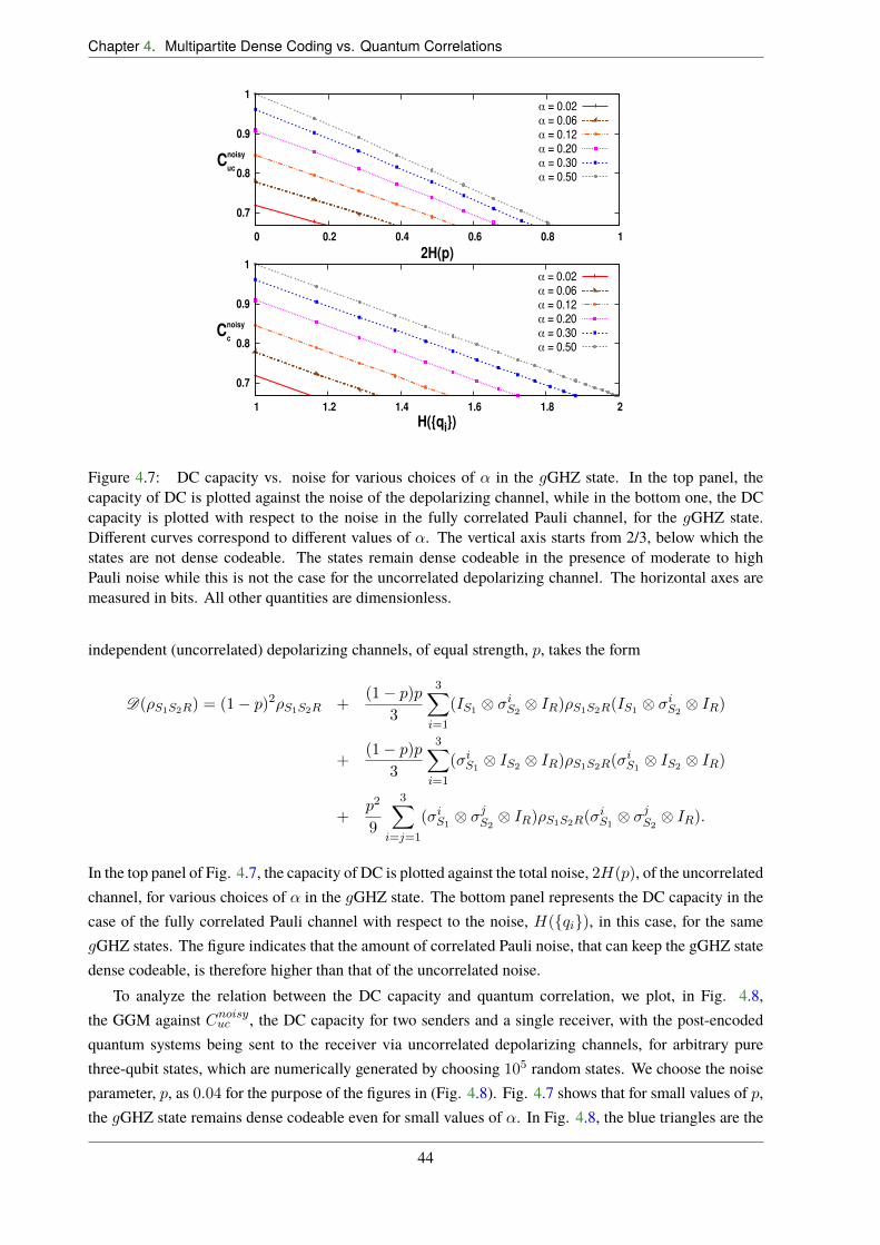
Chapter 4. Multipartite Dense Coding vs. Quantum Correlations

0.7

0.8

0.9

1

1 1.2 1.4 1.6 1.8 2

Cnoisy

c

H({qi})

α = 0.02α = 0.06α = 0.12α = 0.20α = 0.30α = 0.50

0.7

0.8

0.9

1

0 0.2 0.4 0.6 0.8 1

Cnoisy

uc

2H(p)

α = 0.02α = 0.06α = 0.12α = 0.20α = 0.30α = 0.50

Figure 4.7: DC capacity vs. noise for various choices of ↵ in the gGHZ state. In the top panel, thecapacity of DC is plotted against the noise of the depolarizing channel, while in the bottom one, the DCcapacity is plotted with respect to the noise in the fully correlated Pauli channel, for the gGHZ state.Di�erent curves correspond to di�erent values of ↵. The vertical axis starts from 2/3, below which thestates are not dense codeable. The states remain dense codeable in the presence of moderate to highPauli noise while this is not the case for the uncorrelated depolarizing channel. The horizontal axes aremeasured in bits. All other quantities are dimensionless.

independent (uncorrelated) depolarizing channels, of equal strength, p, takes the form

D(⇢S1S2R) = (1� p)2⇢S1S2R +(1� p)p

3

3X

i=1

(IS1 ⌦ �iS2⌦ IR)⇢S1S2R(IS1 ⌦ �

iS2⌦ IR)

+(1� p)p

3

3X

i=1

(�iS1⌦ IS2 ⌦ IR)⇢S1S2R(�

iS1⌦ IS2 ⌦ IR)

+p2

9

3X

i=j=1

(�iS1⌦ �

jS2⌦ IR)⇢S1S2R(�

iS1⌦ �

jS2⌦ IR).

In the top panel of Fig. 4.7, the capacity of DC is plotted against the total noise, 2H(p), of the uncorrelatedchannel, for various choices of ↵ in the gGHZ state. The bottom panel represents the DC capacity in thecase of the fully correlated Pauli channel with respect to the noise, H({qi}), in this case, for the samegGHZ states. The figure indicates that the amount of correlated Pauli noise, that can keep the gGHZ statedense codeable, is therefore higher than that of the uncorrelated noise.

To analyze the relation between the DC capacity and quantum correlation, we plot, in Fig. 4.8,the GGM against Cnoisy

uc , the DC capacity for two senders and a single receiver, with the post-encodedquantum systems being sent to the receiver via uncorrelated depolarizing channels, for arbitrary purethree-qubit states, which are numerically generated by choosing 105 random states. We choose the noiseparameter, p, as 0.04 for the purpose of the figures in (Fig. 4.8). Fig. 4.7 shows that for small values of p,the gGHZ state remains dense codeable even for small values of ↵. In Fig. 4.8, the blue triangles are the

44

4.4. In closing

0

0.1

0.2

0.3

0.4

0.5

0.5 0.55 0.6 0.65 0.7 0.75 0.8 0.85

ε

Cnoisy

uc

Figure 4.8: (Color online.) GGM vs. the raw DC capacity, Cnoisyuc , in the presence of the uncorrelated

noise. See text for further details. Both axes represent dimensionless quantities. The vertical line atC

noisyuc = 2/3 again helps to read the actual capacity from the raw capacity.

ones which satisfy condition (ii) of Theorem 4 and we observe that most of them lie above the red curveof the gGHZ states. Note that condition (i) is not well-defined in the current (uncorrelated) scenario. Theremaining states are represented by orange squares. The similar behavior has also been noticed for theother multiparty QC measures, the tangle and the discord monogamy score.

4.4 In closing

For transmission of classical information over noiseless and memory-less quantum channels, the capacityin the case of a single sender to a single receiver is well-studied. However, point-to-point communication isof limited commercial use and the exploration of quantum networks with multiple senders and receivers istherefore of far greater interest. Moreover, creation of multipartite systems with quantum correlations, theessential ingredient for several quantum communication as well as computational tasks, is currently beingactively pursued in laboratories around the globe. Establishment of connections between multipartitequantum correlation measures and capacities are usually hindered by the unavailability of a uniquemultiparty quantum correlation measure even for pure states, and the plethora of possibilities for multipartycommunication protocols.

For a communication scenario involving several senders and a single receiver, we establish a rela-tion between the capacities of classical information transmission and multipartite computable quantumcorrelation measures, for both noiseless as well as noisy channels. Specifically, we show that there arehierarchies among multipartite states according to the capacities of the dense coding protocol and henceobtain a tool to classify quantum states according to their usefulness in quantum dense coding.

But when one introduces some amount of noise in the transmission channel of the DC protocol ourresults strongly indicate that the relative hierarchies among quantum states, get inverted. The results foundin this chapter are generic in a sense that they seem to be independent of the choices of the multipartiteQC measures as well as for di�erent kinds of noises. A schematic diagram elucidating this phenomena

45

Chapter 4. Multipartite Dense Coding vs. Quantum Correlations

Figure 4.9: Schematic diagram of the change of status of the gGHZ state in comparison to other multipartitestates with respect to multipartite DC capacity in the presence of noise. The comparison has been madewith the states which posses same amount of multipartite quantum correlations as the gGHZ state. Theresults obtained in this paper shows that the gGHZ state is more robust against noise as compared toarbitrary states for the dense coding protocol. This is independent of the fact whether the noise in thesystem is from the source or in the channel after the encoding.

is presented in Fig. 4.9. The results can be an important step forward in building up communicationnetworks using multipartite quantum correlated states in realizable systems.

The results of this Chapter are based on the following paper:

1. Multipartite Dense Coding vs. Quantum Correlation: Noise Inverts Relative Capability of Infor-mation Transfer, Tamoghna Das, R. Prabhu, Aditi Sen De, Ujjwal Sen, Phys. Rev. A 92, 022319(2014).

46

Chapter 5Distributed Quantum Dense coding

In this chapter, we will discuss about the quantum communication network i.e., the protocol of classicalinformation transmission from many senders to two receivers, by using a shared multiparty quantum state.In this protocol, we have assumed that the two receivers are at distant locations and to get the informationor decode the message, they can only perform local quantum operations and classical communication andhence we term this protocol as LOCC-DC protocol. As the ensemble of the encoded states, containingthe information, are distributed among the two receivers, it is also named as the “distributed quantumdense coding” [21,22]. If the two receivers are allowed to come closer and can perform a global quantummeasurement in the entire state space, then the situation reduces to the DC protocol for a single receiverwhich we have already discussed in Chapter 3. The situation of two receivers connected to multiplesenders can be seen in many places in our day to day life – for example, in a big country like India, anewspaper company may have several head o�ces, in particular two major o�ces situated in two di�erentcities that collect news from the field reporters and to print or telecast the news in a coherent manner, thetwo editorial o�ces must know the entire information, by LOCC.

For an arbitrary multiparty quantum state shared between several senders and two receivers, an upperbound on the capacity of distributed DC has been obtained in Ref. [21, 22] in the noiseless scenario.Moreover, it was also shown by giving an explicit LOCC protocol, that the upper bound can be achievedfor a shared four-qubit Greenberger-Horne-Zeilinger (GHZ) state, involving two senders and two receivers.In this chapter, we derive an upper bound on the LOCC-DC, in presence of noise in the transmissionchannel through which the encoded parts are sent to the receivers, for any arbitrary noisy channel. Itcan be further tightened for a particular noise model, namely, the covariant noise [57]. But before goingto this LOCC-DC, we first discuss about how much information, the two party can get, by LOCC whenan ensemble of states are shared between them (locally accessible information) [123, 124]. We start ourdiscussion with the chain rule of mutual information in both classical and quantum domain.

5.1 Chain rule of Mutual information

We first derive the chain rule of mutual information derived in Eq. (2.23) in a classical domain. Suppose,that there is a set of N + 1 random variables X , Y1, Y2, . . . , YN . And their joint probability distribution,

47

Chapter 5. Distributed Quantum Dense coding

p(x, y1, . . . , yN ), of getting X = x and Y1 = y1, . . . , YN = yN , can be written as

p(x, y1, . . . , yN ) = p(x)p(y1, . . . , yN |x) (5.1)

= p(x)p(x, y1, . . . , yN )

p(x, y1, . . . , yN�1)

p(x, y1, . . . , yN�1)

p(x, y1, . . . , yN�2)· · ·

p(x, y1)

p(x)(5.2)

=NY

j=1

p(yj |x, y1, . . . , yj�1)p(x), (5.3)

using Bayes rule of probability distribution [141]. Here, p(yj |x, y1, . . . , yj�1) is the conditional prob-ability of getting Yj = yj , when X = x and Yi = yi, 8i < j has already been occurred. Now theconditional entropy, H(Y1, . . . , YN |X), generalization of Eq. (2.27), for N + 1 random variables tellsus the remaining uncertainty of the random variables Y1, . . . , YN , when one already knows about X andreads as

H(Y1, . . . , YN |X) = �

X

x,y1,...,yN

p(x, y1, . . . , yN ) log2 p(y1, . . . , yN |x) (5.4)

= �

X

x,y1,...,yN

NX

j=1

p(x, y1, . . . , yN ) log2 p(yj |x, y1, . . . , yj�1) (5.5)

=NX

j=1

H(Yj |X,Y1, . . . , Yj�1). (5.6)

Similarly, one can also show that the joint Shannon entropy of random variables Y1, . . . , YN is

H(Y1, . . . , YN ) =NX

j=1

H(Yj |Y1, . . . , Yj�1). (5.7)

The mutual information between X and the set of random variables Y1, . . . , YN , denoted by I(X :

Y1, . . . , YN ) quantifies the information which is common between them, and is given by

I(X : Y1, . . . , YN ) = H(Y1, . . . , YN )�H(Y1, . . . , YN |X) (5.8)

=NX

j=1

H(Yj |Y1, . . . , Yj�1)�H(Yj |X,Y1, . . . , Yj�1) (5.9)

=NX

j=1

I(X : Yj |Y1, . . . , Yj�1). (5.10)

Eq. (5.10) is known as the chain rule of mutual information in classical information theory [141]. In aquantum domain, we assume that the same chain rule of mutual information also holds, where the Shannonentropies are replaced by the von-Neumann entropies.

5.2 Locally accessible information

Suppose that an ensemble E = {px, ⇢xAB} is shared between two parties Alice (A) and Bob (B). Alice

possess the part of the ensemble EA = {px, ⇢

xA} and Bob E

B = {px, ⇢xB}. To know the information

48

5.2. Locally accessible information

Communicate !"!" occur with #$%

{'$%}{#)|$%,,-.

)|$%}

{#)|$%,,-)|$%} {#)|$%,,.

)|$%}

BobAlice

!/occur with #$0|$%$1$2

{#), ,-.) }

{#), ,-)} {#), ,.)}

{'$0}

Communicate !3 !3 occur with #$1|$%{'$1}

{#)|$%$1,,-.)|$%$1}

{#)|$%$1,,.)|$%$1}{#)|$%$1,,-

)|$%$1}

Communicate !4{'$2}

{#)|$%$1$2,,-)|$%$1$2}

!4 occur with #$2|$%$1

{#)|$%$1$2,,-.)|$%$1$2}

{#)|$%$1$2,,.)|$%$1$2}

Figure 5.1: The LOCC protocol of obtaining information about the message x, which occurs withprobability px, when Alice and Bob share an ensemble {px, ⇢

xAB}. First Alice initiates the measurement

on her part of the ensemble and communicates the result to Bob. Depending on the Alice’s outcome, Bobchooses and performs another measurement on the shared post measurement ensemble and communicateshis outcome. The process goes on until they gather maximal information about the ensemble.

about x, Alice and Bob can only perform measurements (PV as well as POVM (see Eqs. (2.30) and(2.31))) in their respective parts of the ensemble, namely on E

A and EB , and communicate their outcome

to the other. Suppose Alice starts the protocol. Alice performs measurement and obtains the result. Shecommunicates her measurement outcome to Bob by classical channel, say by phone call. Depending onthe measurement outcome of Alice, Bob chooses his measurement and again communicates to Alice. Theprocess goes on until the two party gather as much information as possible about the shared ensemble.

Suppose, Alice first performs measurement, {My1}, on her part of the quantum state, obtains theoutcome y1 with the probability py1 , creates the post measurement ensemble (PME) {px|y1 , ⇢

x|y1AB }, shared

between Alice and Bob. After Alice’s measurement, and her communication to Bob, the part of theensemble in Bob’s possession also changes as depicted in Fig. 5.1. Bob next performs measurement,{My2}, in his part of the PME, and obtains the result, say, y2 which occurs with probability py2|y1 ,resulting PME {px|y1y2 , ⇢

x|y1y2AB }. The outcome has again been communicated to Alice and she performs

49

Chapter 5. Distributed Quantum Dense coding

another measurement and then communicates her result to Bob and so on, as depicted in Fig. 5.1.Let us now ask the question. How much information these two parties can gather after this LOCC

protocol ? To find the answer of this question, we will use the chain rule of mutual information, as givenin Eq. (5.10), where the random variable X will be replaced by the initial ensemble and Y1, Y2, . . . arethe measurement outcomes of the Alice’s and Bob’s measurements denoted by {Myi}.

5.2.1 Information gain in a single measurement

Before discussing the information gain by a general LOCC protocol, let us discuss the maximal informationobtained by two parties, when one of them performs a measurement on a given ensemble. For ashared ensemble {px, ⇢

xAB}, the ensemble which Alice can manipulate is E

A. Suppose, she performsmeasurement {My1} on her part of the ensemble. The question is how much information Alice can gainafter this single measurement. In this section, we will address this question and derive the informationaccessible after a measurement [123, 185]. For the sake of simplicity, the subscript A has been omittedfrom the ensemble of state in the rest of the subsection.

Any ensemble of states {px, ⇢x} can be considered as a part of a larger system, ⇢XSY , given by

⇢XSY =X

x

px|xihx|X ⌦ ⇢xS ⌦ |0ih0|Y , (5.11)

where S represents our system of interest, {|xi} is a set of orthogonal basis in the system X , whichexhausts all the possible preparation of ⇢x and can be considered as a register of ⇢x. Here, |0i is the intialstate of an ancillary system Y . Now any measurement {My}1 on the system S can be considered as acomposite operation on the joint Hilbert space of SY [135], i.e.,

⇢0XSY =

X

x

px|xihx|X ⌦X

y

My⇢xSM

†y ⌦ |yihy|Y , (5.12)

withP

y M†yMy = IY and |yi is a orthogonal basis in the ancillary system Y , with the same number of

elements as {My}. Here, My⇢xSM

†y , is not a trace preserving operation, and

py|x = tr�My⇢

xSM

†y

�(5.13)

is the probability of getting the outcomeY = y, when the given state is ⇢x, and hence the post measurementstate is given by

⇢x|y = My⇢

xSM

†y/py|x. (5.14)

The state in Eq. (5.12), can be rewritten as

⇢0XSY =

X

xy

pxpy|x|xihx|X ⌦ ⇢x|yS ⌦ |yihy|Y , (5.15)

=X

y

py

X

x

px|y|xihx|X ⌦ ⇢x|yS ⌦ |yihy|Y . (5.16)

Here we use the Bayes rule [141] of probability theory. The above equation is the averaged total state,when no one has bothered about the outcome of the measurement. But if the outcome is known, then the

1We also skip the subscript 1 in {My} in Alice’s measurement.

50

5.2. Locally accessible information

initial ensemble reduces to an ensemble {px|y, ⇢x|y} occurring with probability py.

The amount of information gained, in this measurement, is the quantum mutual information of the state⇢0XY . Since, the information of the initial ensemble is registered in the basis {|xiX} and the measurement

outcome in the basis {|yiY }. From the chain rule of mutual information of ⇢0XSY , in the X : SY

bipartition, given in Eq. (5.10), we have

I(⇢0X:SY ) = I(⇢0X:Y ) + I(⇢0X:S|Y ). (5.17)

But the mutual information is non-increasing under local operations [135], so we get

I(⇢0X:SY ) I(⇢X:SY ) = I(⇢X:S). (5.18)

The last equality holds due to the fact that the system Y is in a product form with XS, in ⇢XSY , as shownin Eq. (5.11). Therefore,

I(⇢X:S) = S(⇢X) + S(⇢S)� S(⇢XS), (5.19)

= H(X) + S

⇣X

x

px⇢x⌘� S(⇢XS), (5.20)

where H(X) = �P

x px log2 px, is the Shannon entropy of {px}. To calculate S(⇢XS), we diagonaliseeach ⇢x =

Pµ �

xµ|µ

xihµ

x|, with the mutually orthogonal eigenvector |µx

i corresponding to the eigenvalue�xµ, and hence

⇢XS =X

x

px|xihx|X ⌦X

µ

�xµ|µ

xihµ

x|S . (5.21)

The von-Neumann entropy then reduces to

S(⇢XS) = �

X

xµ

px�xµ log2(px�

xµ)

= �

X

xµ

�xµ px log2 px �

X

x

px

X

µ

�xµ log2 �

xµ

= H(X) +X

x

pxS(⇢x). (5.22)

The mutual information is then given by

I(⇢X:S) = S

⇣X

x

px⇢x⌘�

X

x

pxS(⇢x) = �

S, (5.23)

the Holevo quantity of a given ensemble {px, ⇢x}, as given in Eq. (3.2). The second term in Eq. (5.17) isdefined as

I(⇢0X:S|Y ) =X

y

pyI(⇢0X:S|Y=y), (5.24)

where⇢0X:S|Y=y =

X

x

px|y|xihx|X ⌦ ⇢x|yS ⌦ |yihy|Y . (5.25)

51

Chapter 5. Distributed Quantum Dense coding

So we haveI(⇢0X:S|Y ) =

X

y

py

hS

⇣X

x

px|y⇢x|y⌘�

X

x

px|yS(⇢x|y)

i= �

S. (5.26)

Combining the results in Eqs. (5.17), (5.18), (5.23) and (5.26), the information accessible to Alice, afterher first measurement on the shared ensemble {px, ⇢xAB}2, is given by

I(⇢0X:Y ) ⌘ IA1 �

A� �

A, (5.27)

where

�A = S

⇣X

x

px⇢xA

⌘�

X

x

pxS�⇢xA

�, (5.28)

�A =

X

y

py

hS

⇣X

x

px|y⇢x|yA

⌘�

X

x

px|yS�⇢x|yA

�i. (5.29)

5.2.2 Information gain in successive measurements

Suppose now that Alice and Bob have performed total N number of local measurements Y1, Y2, . . . , YNsuccessively, where all the odd number of measurements are done by Alice and all the even numberof measurements are by Bob. Moreover, it is assumed that after each measurement, both of themsuccessfully communicated their results, to the other one and except the first one, all the measurement arechosen depending on the previous measurements results. The information gain in this scenario can bequantified from the joint mutual information as

I(⇢X:Y1,Y2,...,YN) =

NX

j=1

I(⇢X:Yj |Y1,...,Yj�1) (5.30)

= I(⇢X:Y1) + I(⇢X:Y2|Y1) + · · ·+ I(⇢X:YN |Y1,...,YN�1

), (5.31)

where we use Eq. (5.10). Here we assume that Alice initiates the first measurement {My1}, as shown inFig. 5.1, and the information she obtained, according to Eq. (5.27), is given by

I(⇢X:Y1) �A1 � �

A1 , (5.32)

where ‘1’ in the subscript indicates the first measurement {My1}. On the other hand, the accessibleinformation by Bob after his measurement {My2} is given by

I(⇢X:Y2|Y1)

X

y1

py1

⇥�B2 � �

B2

⇤. (5.33)

where py1 is the probability of obtaining the outcome y1 by Alice in the measurement {My1}. Similarly,after Alice’s second measurement {My3}, we get

I(⇢X:Y3|Y1,Y2)

X

y1y2

py1y2

⇥�A3 � �

A3

⇤. (5.34)

2 This is the information gain by Alice and Bob after a single measurement performed by Alice and without any classicalcommunication to Bob. Of course, similar result can be obtained if Bob starts the protocol, replacing superscript “A” by “B” inEq. (5.27)

52

5.2. Locally accessible information

and so on. Here �A1 and �A

1 is given in Eqs. (5.28) and (5.29), and

�B2 = S

⇣X

x

px|y1⇢x|y1B

⌘�

X

x

px|y1S�⇢x|y1B

�(5.35)

�B2 =

X

y2

py2|y1

hS

⇣X

x

px|y1y2⇢x|y1y2B

⌘�

X

x

px|y1y2S�⇢x|y1y2B

�i(5.36)

�A3 = S

⇣X

x

px|y1y2⇢x|y1y2A

⌘�

X

x

px|y1y2S�⇢x|y1y2A

�(5.37)

�A3 =

X

y3

py3|y1y2

hS

⇣X

x

px|y1y2y3⇢x|y1y2y3A

⌘�

X

x

px|y1y2y3S�⇢x|y1y2y3A

�i. (5.38)

Notice that any measurement in Alice’s subsystem does not change the average density matrix in theBob’s part, or vice-versa. Mathematically, we have

X

y1

py1

X

x

px|y1⇢x|y1B =

X

x

pxtrA⇣X

y1|x

py1|xMy1 ⌦ IB⇢xABM

†y1 ⌦ IB

⌘ 1

py1|x, (5.39)

=X

x

px⇢xB. (5.40)

Similarly, we also have

X

y2

py2|y1X

x

px|y1y2⇢x|y1y2A =

X

x

px|y1⇢x|y1A , (5.41)

X

y3

py3|y1y2X

x

px|y1y2y3⇢x|y1y2y3B =

X

x

px|y1y2⇢x|y1y2B , (5.42)

X

y4

py4|y1y2y3X

x

px|y1y2y3y4⇢x|y1y2y3y4A =

X

x

px|y1y2y3⇢x|y1y2y3A . (5.43)

Now define

⇢A =X

x

px⇢xA, (5.44)

SxA =

X

x

pxS(⇢xA), (5.45)

Sx|1A =

X

xy1

pxy1S(⇢x|y1A ), (5.46)

andSx|nA =

X

xy1...yn

pxy1...ynS(⇢x|y1...ynA ). (5.47)

Similarly, one can write, replacing A by B. Putting all the terms in Eq. (5.30), we obtain the accessibleinformation under LOCC performed by both Alice and Bob as

ILOCCacc

hS(⇢A)� S

xA �

X

y1

py1S

⇣X

x

px|y1⇢x|y1A

⌘+ S

x|1A

i

+hS(⇢B)� S

x|1B �

X

y1y2

py1y2S

⇣X

x

px|y1y2⇢x|y1y2B

⌘+ S

x|2B

i

53

Chapter 5. Distributed Quantum Dense coding

+hX

y1y2

py1y2S

⇣X

x

px|y1y2⇢x|y1y2A

⌘� S

x|2A �

X

y1y2y3

py1y2y3S

⇣X

x

px|y1y2y3⇢x|y1y2y3A

⌘+ S

x|3A

i

+h X

y1y2y3

py1y2y3S

⇣X

x

px|y1y2y3⇢x|y1y2y3B

⌘+ · · · (5.48)

S(⇢A)� SxA + S

x|1A + S(⇢B)� S

x|1B + S

x|2B � S

x|2A + S

x|3A � S

x|3B + S

x|4B + · · · (5.49)

= S(⇢A) + S(⇢B)� SxB �

�SxA � S

x|1A �

�SxB � S

x|1B

� +�Sx|2A � S

x|3A �

�Sx|2B � S

x|3B

�

+ · · · . (5.50)

Here we use the concavity and the positivity of von-Neumann entropy, in the following terms :

X

y1

py1S

⇣X

x

px|y1⇢x|y1B

⌘ S

⇣X

xy1

py1px|y1⇢x|y1B

⌘(5.51)

X

y1y2

py1y2S

⇣X

x

px|y1y2⇢x|y1y2B

⌘

X

y1

py1S

⇣X

y2

py2|y1X

x

px|y1y2⇢x|y1y2B

⌘(5.52)

X

y1y2y3

py1y2y3S

⇣X

x

px|y1y2y3⇢x|y1y2y3B

⌘

X

y1y2

py1y2S

⇣X

y3

py3|y1y2X

x

px|y1y2y3⇢x|y1y2y3B

⌘(5.53)

and use Eqs. (5.41), (5.42) and (5.43) to get the form of Eq. (5.49). Let us now use another fact that theaverage entropic change in the measured party is always bounded above by average entropic change in theunmeasured party. Mathematically,

SxA � S

x|1A � S

xB � S

x|1B , (5.54)

Sx|2A � S

x|3A � S

x|2B � S

x|3B . (5.55)

The above bound can be proved if one considers the purification of the initial ensemble {px, ⇢xAB}, as

{px, | xABCi}, where

⇢xAB = trC | x

ABCih xABC |, (5.56)

by adding an ancilla C in the unmeasured part. Now any measurement {My} by Alice, with outcome y,occurring with py, on the pure state ensemble leaves the PME as {px|y, |

x|yABCi},

| xABCi �!My ⌦ IBC |

xABCi/py|x = |

x|yABCi, (5.57)

with py|x = h xABC |M

†yMy ⌦ IBC |

xABCi. Finally, we have

X

x

pxS�⇢xA

��

X

xy1

pxy1S(⇢x|y1A ) =

X

x

pxS�⇢xBC

��

X

xy1

pxy1S(⇢x|y1BC )

�

X

x

pxS�⇢xB

��

X

xy1

pxy1S(⇢x|y1B ). (5.58)

The last inequality comes from the fact that Holevo quantity is non-increasing under discarding thesubsystem.Hence, all the terms in the parentheses of Eq. (5.50) are non-positive, and therefore, we obtain

ILOCCacc S(⇢A) + S(⇢B)� S

xB. (5.59)

54

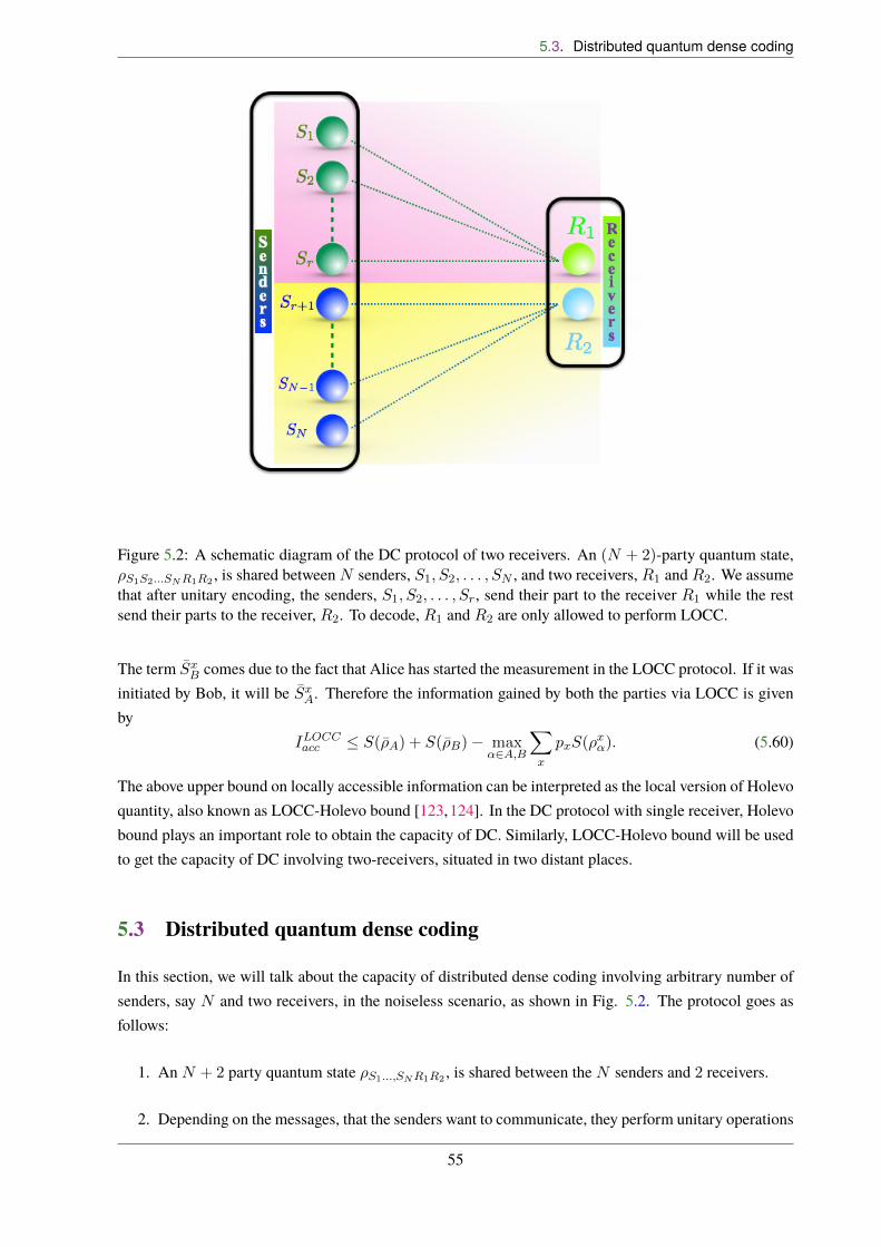
5.3. Distributed quantum dense coding

Figure 5.2: A schematic diagram of the DC protocol of two receivers. An (N + 2)-party quantum state,⇢S1S2...SNR1R2 , is shared between N senders, S1, S2, . . . , SN , and two receivers, R1 and R2. We assumethat after unitary encoding, the senders, S1, S2, . . . , Sr, send their part to the receiver R1 while the restsend their parts to the receiver, R2. To decode, R1 and R2 are only allowed to perform LOCC.

The term SxB comes due to the fact that Alice has started the measurement in the LOCC protocol. If it was

initiated by Bob, it will be SxA. Therefore the information gained by both the parties via LOCC is given

byILOCCacc S(⇢A) + S(⇢B)� max

↵2A,B

X

x

pxS(⇢x↵). (5.60)

The above upper bound on locally accessible information can be interpreted as the local version of Holevoquantity, also known as LOCC-Holevo bound [123,124]. In the DC protocol with single receiver, Holevobound plays an important role to obtain the capacity of DC. Similarly, LOCC-Holevo bound will be usedto get the capacity of DC involving two-receivers, situated in two distant places.

5.3 Distributed quantum dense coding

In this section, we will talk about the capacity of distributed dense coding involving arbitrary number ofsenders, say N and two receivers, in the noiseless scenario, as shown in Fig. 5.2. The protocol goes asfollows:

1. An N + 2 party quantum state ⇢S1...,SNR1R2 , is shared between the N senders and 2 receivers.

2. Depending on the messages, that the senders want to communicate, they perform unitary operations

55

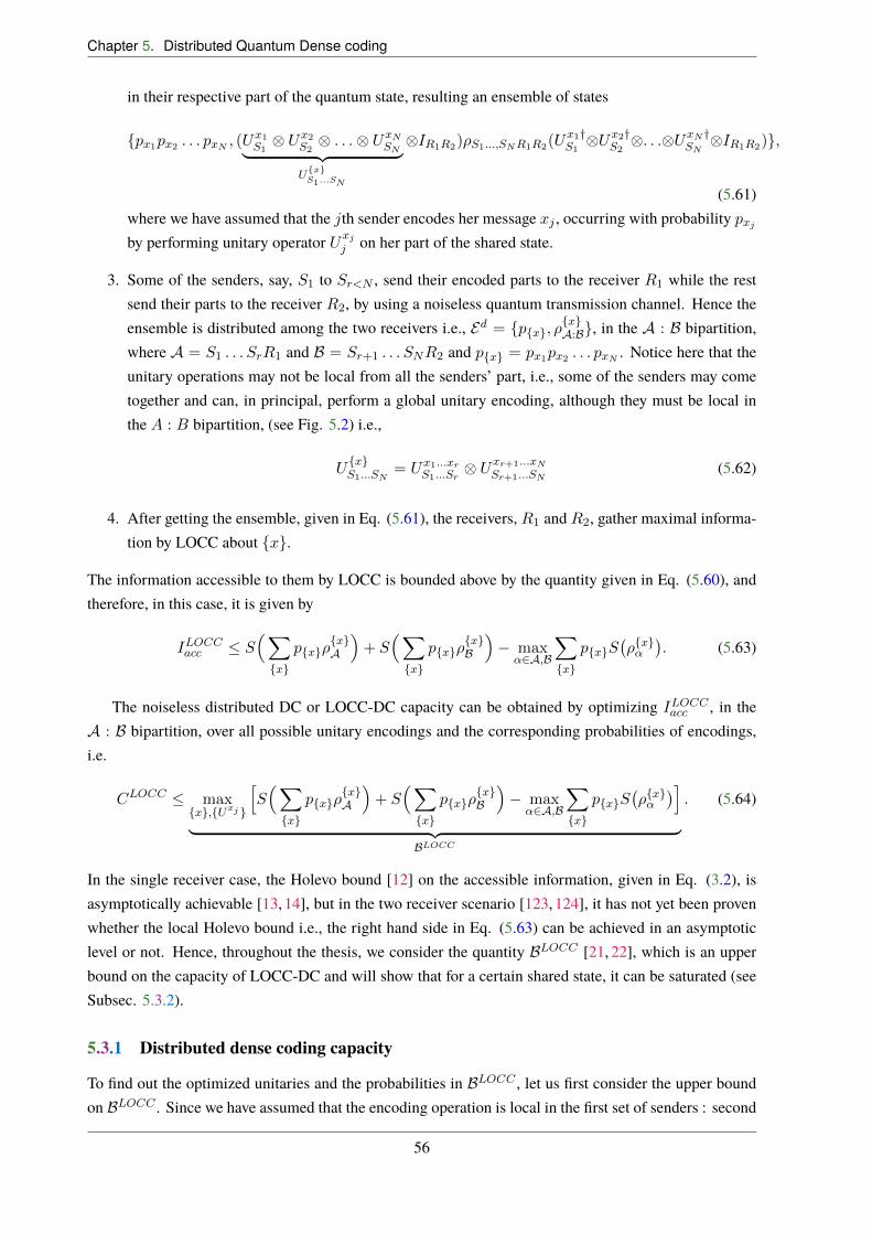
Chapter 5. Distributed Quantum Dense coding

in their respective part of the quantum state, resulting an ensemble of states

{px1px2 . . . pxN, (Ux1

S1⌦ U

x2S2⌦ . . .⌦ U

xN

SN| {z }U

{x}S1...SN

⌦IR1R2)⇢S1...,SNR1R2(Ux1†S1⌦U

x2†S2⌦. . .⌦U

xN †SN⌦IR1R2)},

(5.61)where we have assumed that the jth sender encodes her message xj , occurring with probability pxj

by performing unitary operator Uxj

j on her part of the shared state.

3. Some of the senders, say, S1 to Sr<N , send their encoded parts to the receiver R1 while the restsend their parts to the receiver R2, by using a noiseless quantum transmission channel. Hence theensemble is distributed among the two receivers i.e., Ed = {p{x}, ⇢

{x}A:B}, in the A : B bipartition,

where A = S1 . . . SrR1 and B = Sr+1 . . . SNR2 and p{x} = px1px2 . . . pxN. Notice here that the

unitary operations may not be local from all the senders’ part, i.e., some of the senders may cometogether and can, in principal, perform a global unitary encoding, although they must be local inthe A : B bipartition, (see Fig. 5.2) i.e.,

U{x}S1...SN

= Ux1...xr

S1...Sr⌦ U

xr+1...xN

Sr+1...SN(5.62)

4. After getting the ensemble, given in Eq. (5.61), the receivers, R1 and R2, gather maximal informa-tion by LOCC about {x}.

The information accessible to them by LOCC is bounded above by the quantity given in Eq. (5.60), andtherefore, in this case, it is given by

ILOCCacc S

⇣X

{x}

p{x}⇢{x}A

⌘+ S

⇣X

{x}

p{x}⇢{x}B

⌘� max↵2A,B

X

{x}

p{x}S�⇢{x}↵

�. (5.63)

The noiseless distributed DC or LOCC-DC capacity can be obtained by optimizing ILOCCacc , in the

A : B bipartition, over all possible unitary encodings and the corresponding probabilities of encodings,i.e.

CLOCC

max{x},{Uxj }

hS

⇣X

{x}

p{x}⇢{x}A

⌘+ S

⇣X

{x}

p{x}⇢{x}B

⌘� max↵2A,B

X

{x}

p{x}S�⇢{x}↵

�i

| {z }BLOCC

. (5.64)

In the single receiver case, the Holevo bound [12] on the accessible information, given in Eq. (3.2), isasymptotically achievable [13, 14], but in the two receiver scenario [123, 124], it has not yet been provenwhether the local Holevo bound i.e., the right hand side in Eq. (5.63) can be achieved in an asymptoticlevel or not. Hence, throughout the thesis, we consider the quantity B

LOCC [21, 22], which is an upperbound on the capacity of LOCC-DC and will show that for a certain shared state, it can be saturated (seeSubsec. 5.3.2).

5.3.1 Distributed dense coding capacity

To find out the optimized unitaries and the probabilities in BLOCC , let us first consider the upper bound

on BLOCC . Since we have assumed that the encoding operation is local in the first set of senders : second

56

5.3. Distributed quantum dense coding

set of senders bipartition we have

S(⇢{x}A ) = S�U

x1...xr

S1...Sr⌦ IR1 ⇢

{x}A U

x1...xr†S1...Sr

⌦ IR1

�= S(⇢A), (5.65)

S(⇢{x}B ) = S�U

xr+1...xN

Sr+1...SN⌦ IR2 ⇢

{x}B U

xr+1...xN †Sr+1...SN

⌦ IR2

�= S(⇢B), (5.66)

and hence the last term of Eq. (5.63) reduces to

max↵2A,B

X

{x}

p{x}S�⇢{x}↵

�= max

↵2A,BS(⇢↵). (5.67)

If we now apply the subadditivity of von-Neumann entropy in the first term of Eq. (5.63) in theS1 . . . Sr : R1, bipartition, we get

S

⇣X

{x}

p{x}⇢{x}A

⌘ S

⇣X

{x}

p{x}⇢{x}S1...Sr

⌘+ S

⇣X

{x}

p{x}⇢{x}R1

⌘

log2 dS1...Sr+ S(⇢R1). (5.68)

In the last inequality we use that the von-Neumann entropy of the quantum state of the first set of sendersis bounded above of the logarithm of the dimension of the sender’s system with dS1...Sr

= dS1 ·dS2 · · · dSr

being the dimensions of the first set of senders and ⇢{x}R1= ⇢R1 , 8{x} since as there is no unitary acting

on the receivers system. Similarly, we obtain

S

⇣X

{x}

p{x}⇢{x}B

⌘ log2 dSr+1...SN

+ S(⇢R2). (5.69)

Hence we have

BLOCC

log2 dS1...Sr+ log2 dSr+1...SN

+ S(⇢R1) + S(⇢R2)� max↵2A,B

S(⇢↵). (5.70)

It can be shown [21] that this upper bound can be achieved by choosing a complete set of orthogonal

unitaries {W ijSj}

d2Sj�1

i=0 (see Eqs. (3.8) and (3.9)) where the encoding operation on the jth sender occurswith equal probability pij =

1d2Sj

. For all the senders, we have

U{x}S1,...,SN

=NO

j=1

WijSj, p{x} =

1QN

j=1 d2Sj

. (5.71)

Hence, the upper bound on the LOCC-DC capacity reduces to

BLOCC = log2 dS1...SN

+ S(⇢R1) + S(⇢R2)� max↵2A,B

S(⇢↵). (5.72)

5.3.2 Distributed DC with four-qubit GHZ state

In this subsection, the upper bound on the capacity of distributed quantum DC or LOCC-DC, BLOCC , canbe achieved for a particular example of shared state. Let us consider a four-qubit GHZ [56] state, given by

|GHZiS1S2R1R2 =1p2(|00iS1S2 |00iR1R2 + |11iS1S2 |11iR1R2), (5.73)

57

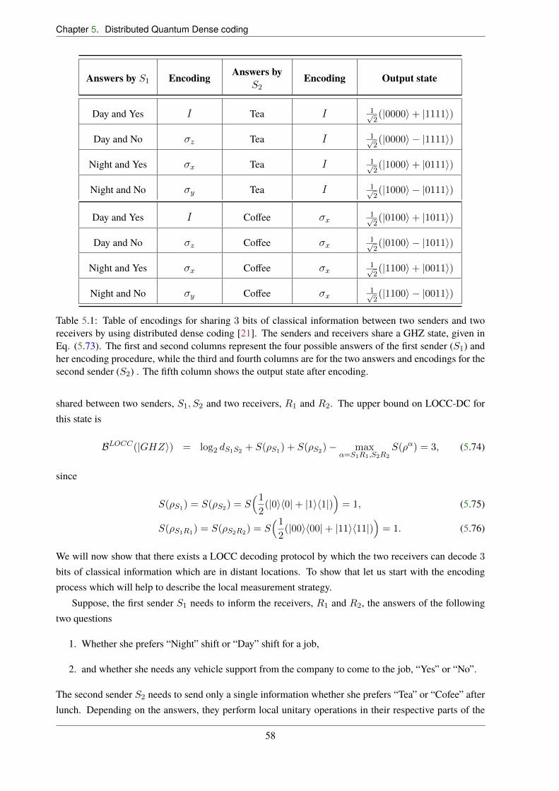
Chapter 5. Distributed Quantum Dense coding

Answers by S1 Encoding Answers byS2

Encoding Output state

Day and Yes I Tea I 1p2(|0000i+ |1111i)

Day and No �z Tea I 1p2(|0000i � |1111i)

Night and Yes �x Tea I 1p2(|1000i+ |0111i)

Night and No �y Tea I 1p2(|1000i � |0111i)

Day and Yes I Co�ee �x1p2(|0100i+ |1011i)

Day and No �z Co�ee �x1p2(|0100i � |1011i)

Night and Yes �x Co�ee �x1p2(|1100i+ |0011i)

Night and No �y Co�ee �x1p2(|1100i � |0011i)

Table 5.1: Table of encodings for sharing 3 bits of classical information between two senders and tworeceivers by using distributed dense coding [21]. The senders and receivers share a GHZ state, given inEq. (5.73). The first and second columns represent the four possible answers of the first sender (S1) andher encoding procedure, while the third and fourth columns are for the two answers and encodings for thesecond sender (S2) . The fifth column shows the output state after encoding.

shared between two senders, S1, S2 and two receivers, R1 and R2. The upper bound on LOCC-DC forthis state is

BLOCC(|GHZi) = log2 dS1S2 + S(⇢S1) + S(⇢S2)� max

↵=S1R1,S2R2

S(⇢↵) = 3, (5.74)

since

S(⇢S1) = S(⇢S2) = S

⇣12(|0ih0|+ |1ih1|)

⌘= 1, (5.75)

S(⇢S1R1) = S(⇢S2R2) = S

⇣12(|00ih00|+ |11ih11|)

⌘= 1. (5.76)

We will now show that there exists a LOCC decoding protocol by which the two receivers can decode 3

bits of classical information which are in distant locations. To show that let us start with the encodingprocess which will help to describe the local measurement strategy.

Suppose, the first sender S1 needs to inform the receivers, R1 and R2, the answers of the followingtwo questions

1. Whether she prefers “Night” shift or “Day” shift for a job,

2. and whether she needs any vehicle support from the company to come to the job, “Yes” or “No”.

The second sender S2 needs to send only a single information whether she prefers “Tea” or “Cofee” afterlunch. Depending on the answers, they perform local unitary operations in their respective parts of the

58

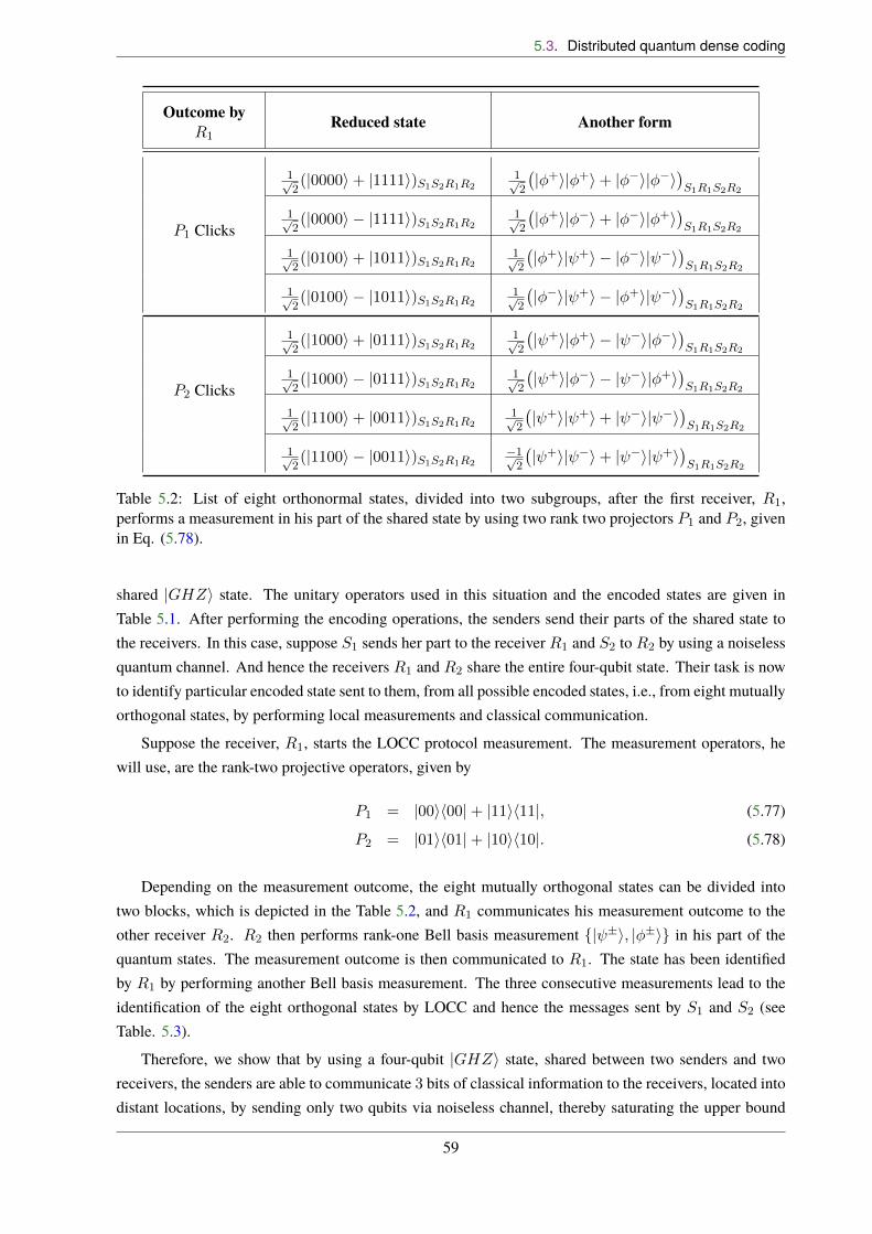
5.3. Distributed quantum dense coding

Outcome byR1

Reduced state Another form

P1 Clicks

1p2(|0000i+ |1111i)S1S2R1R2

1p2

�|�

+i|�

+i+ |�

�i|��i�S1R1S2R2

1p2(|0000i � |1111i)S1S2R1R2

1p2

�|�

+i|��i+ |�

�i|�

+i�S1R1S2R2

1p2(|0100i+ |1011i)S1S2R1R2

1p2

�|�

+i|

+i � |�

�i| �i�S1R1S2R2

1p2(|0100i � |1011i)S1S2R1R2

1p2

�|��i|

+i � |�

+i| �i�S1R1S2R2

P2 Clicks

1p2(|1000i+ |0111i)S1S2R1R2

1p2

�|

+i|�

+i � |

�i|��i�S1R1S2R2

1p2(|1000i � |0111i)S1S2R1R2

1p2

�|

+i|��i � |

�i|�

+i�S1R1S2R2

1p2(|1100i+ |0011i)S1S2R1R2

1p2

�|

+i|

+i+ |

�i| �i�S1R1S2R2

1p2(|1100i � |0011i)S1S2R1R2

�1p2

�|

+i| �i+ |

�i|

+i�S1R1S2R2

Table 5.2: List of eight orthonormal states, divided into two subgroups, after the first receiver, R1,performs a measurement in his part of the shared state by using two rank two projectors P1 and P2, givenin Eq. (5.78).

shared |GHZi state. The unitary operators used in this situation and the encoded states are given inTable 5.1. After performing the encoding operations, the senders send their parts of the shared state tothe receivers. In this case, suppose S1 sends her part to the receiver R1 and S2 to R2 by using a noiselessquantum channel. And hence the receivers R1 and R2 share the entire four-qubit state. Their task is nowto identify particular encoded state sent to them, from all possible encoded states, i.e., from eight mutuallyorthogonal states, by performing local measurements and classical communication.

Suppose the receiver, R1, starts the LOCC protocol measurement. The measurement operators, hewill use, are the rank-two projective operators, given by

P1 = |00ih00|+ |11ih11|, (5.77)

P2 = |01ih01|+ |10ih10|. (5.78)

Depending on the measurement outcome, the eight mutually orthogonal states can be divided intotwo blocks, which is depicted in the Table 5.2, and R1 communicates his measurement outcome to theother receiver R2. R2 then performs rank-one Bell basis measurement {| ±

i, |�±i} in his part of the

quantum states. The measurement outcome is then communicated to R1. The state has been identifiedby R1 by performing another Bell basis measurement. The three consecutive measurements lead to theidentification of the eight orthogonal states by LOCC and hence the messages sent by S1 and S2 (seeTable. 5.3).

Therefore, we show that by using a four-qubit |GHZi state, shared between two senders and tworeceivers, the senders are able to communicate 3 bits of classical information to the receivers, located intodistant locations, by sending only two qubits via noiseless channel, thereby saturating the upper bound

59

Chapter 5. Distributed Quantum Dense coding

Outcome of 1stmeasurement by

R1

Outcome of 2ndmeasurement by

R2

Outcome of 3rdmeasurement by

R1

Conclusion

P1 Clicks

|�+i |�

+i 1p

2(|0000i+ |1111i)

|��i |�

�i

|��i |�

+i 1p

2(|0000i � |1111i)

|�+i |�

�i

| +i |�

+i 1p

2(|0100i+ |1011i)

| �i |�

�i

| +i |�

�i 1p

2(|0100i � |1011i)

| �i |�

+i

P2 Clicks

|�+i |

+i 1p

2(|1000i+ |0111i)

|��i |

�i

|��i |

+i 1p

2(|1000i � |0111i)

|�+i |

�i

| +i |

+i 1p

2(|1100i+ |0011i)

| �i |

�i

| �i |

+i 1p

2(|1100i � |0011i)

| +i |

�i

Table 5.3: Table of the LOCC decoding protocol by the two receivers R1 and R2. The first columnrepresents the outcome of the 1st measurement by R1. The second column represents the measurementoutcomes of the receiver R2 , depending on the measurement outcome of R1. The third column is thethird measurement which is performed by R1 after knowing the outcomes of R2. The second and thirdmeasurements performed byR2 andR1 respectively are the Bell basis measurements, {| ±

i, |�±i}. After

all the measurements, the receivers can finally distinguish all the eight orthonormal states as mentionedin the fourth column.

BLOCC , given in Eq. (5.74). We note that the classical limit in this case is log2 4 = 2, where 4 is the

dimension of the senders’ subsystem and hence by the GHZ state, we obtain quantum advantage in LOCCprotocol.

For the same shared state, i.e., the |GHZi, if the receivers are not allowed to communicate betweeneach other, the protocol can be considered as two distinct dense coding protocols involving a bipartitemixed state ⇢S1R1 and ⇢S2R2 shared between the respective senders and the receivers. It can be shown thatthe DC capacity in this case is not more than 2, which coincides with the classical limit. And hence forthat shared state, the LOCC-DC protocol is more advantageous than the individual dense coding protocolson the DC protocol by LO.

This is also evident from the expression of the multiparty DC capacity. If the two receivers do notcommunicate between each other, then it can be considered as two distinct DC protocols between twoblocks of senders and receivers, (pink and yellow blocks as shown in Fig. (5.2)), and their collective DC

60

5.4. Distributed DC in presence of noisy quantum channels

capacity is

Ccollective =

�log2 dS1...Sr

+ S(⇢R1)� S(⇢A)⌘+⇣log2 dSr+1...SN

+ S(⇢R2)� S(⇢B)⌘. (5.79)

The collective DC capacity is smaller than the LOCC-DC capacity, given in Eq. (5.72) sincemin↵2A,B S(⇢↵) �

0, assuming that the upper bound can be reached as it is the case for the shared |GHZi state. The sameordering remains, if the shared state ⇢S1...SNR1R2 is a product of the form ⇢A ⌦ ⇢B, expect when it is apure product, for which C

collective = BLOCC .

5.4 Distributed DC in presence of noisy quantum channels

In this section, our aim is to estimate the capacity of distributed quantum DC, for the shared N + 2 partyquantum state, ⇢S1,...,SN ,R1,R2 , when the senders send their encoded parts of the shared quantum stateto the respective receivers by using a general noisy quantum channel. In particular, a system can not bekept completely isolated from the environment and hence noise will inevitably interact with the system,thereby changing the form of the encoded state. As we have already discussed in Sec. 3.2.1, noise in thetransmission channel can be characterized by a CPTP map, ⇤, acting on the state space of the senders’ partof the transmitted state. Therefore, the receivers, R1 and R2, after the transmission, possess the distortedensemble,

Ednoisy = {p{x},⇤S1...SN

(⇢{x}S1...SNR1R2)}, (5.80)

in the same S1 . . . SrR1 : Sr+1 . . . SNR2 = A : B bipartition, where

⇤S1...SN

�⇢{x}S1...SNR1R2

�= ⇤S1...SN

�(Ux1...xr

S1...Sr⌦ U

xr+1...xN

Sr+1...SN⌦ IR1R2) ⇢S1...SNR1R2

(Ux1...xr†S1...Sr

⌦ Uxr+1...xN †Sr+1...SN

⌦ IR1R2)�

(5.81)

Now we will try to find out the upper bound on the noisy BLOCC , for any arbitrary noisy quantum channel

⇤, which is also an upper bound on distributed DC capacity.

5.4.1 Upper bound on LOCC-DC for arbitrary noisy channel

To estimate the capacity, let us consider the (N + 2)-party quantum state, ⇢S1...SNR1R2 , which can beexpanded as

⇢S1...SNR1R2 =X

{i,j}

�{i,j}|i1ihj1|S1...SN⌦ |i2ihj2|R1 ⌦ |i3ihj3|R2 , (5.82)

where {|i1i}dS1...SN

�1i1=0 , {|i2i}

dR1�1i2=0 , and {|i3i}

dR2�1i3=0 are respectively bases in the Hilbert space HS1...SN ,

of all the senders, and HR1 (HR2) of the receiver R1 (R2).

After the action of the CPTP map, ⇤, on the encoded state, we get

⇤S1...SN(⇢{x}S1...SNR1R2

) =X

{i,j}

�{i,j}⇤S1...SN

�(Ux1...xr

S1...Sr⌦ U

xr+1...xN

Sr+1...SN) |i1ihj1|S1...SN

(Ux1...xr†S1...Sr

⌦ Uxr+1...xN †Sr+1...SN

)�

⌦|i2ihj2|R1 ⌦ |i3ihj3|R2 , (5.83)

61

Chapter 5. Distributed Quantum Dense coding

where ⇤S1...SNis collectively or individually acting only on the senders’ subsystems. From Eq.

(5.60), we know that the amount of classical information that can be extracted from the ensemble,{p{x},⇤S1...SN

(⇢{x}S1...SNR1R2)}, by LOCC, is given by

ILOCCacc S

⇣X

{x}

p{x}⇠{x}A

⌘+ S

⇣X

{x}

p{x}⇠{x}B

⌘� max↵2A:B

X

{x}

p{x}S�⇠{x}↵

�, (5.84)

where ⇠{x}A = trB⇣⇤�⇢{x}S1...SNR1R2

�⌘and ⇠{x}B = trA

⇣⇤�⇢{x}S1...SNR1R2

�⌘. Like in the noiseless case, to

obtain the capacity of LOCC-DC in a noisy scenario, one has to maximize the R.H.S. of (5.84) overunitaries and probabilities. The ensemble, in the noisy scenario, involves the CPTP map ⇤.

CLOCCnoisy max

{x},{Uxj }

hS

⇣X

{x}

p{x}⇠{x}A

⌘+ S

⇣X

{x}

p{x}⇠{x}B

⌘� max↵2A:B

X

{x}

p{x}S�⇠{x}↵

�i

| {z }�LOCCnoisy

(5.85)

If we apply the subadditivity of von Neumann entropy in the S1 . . . Sr : R1 and Sr+1 . . . SN : R2

bipartitions for the first two terms of �LOCCnoisy , we have

S

⇣X

{x}

p{x}⇠{x}↵

⌘ S

⇣X

{x}

p{x}⇠{x}Rk

⌘+ S

⇣X

{x}

p{x}⇠{x}Rk

⌘

log2 dRk+ S(⇢Rk

), k = 1, 2. (5.86)

where ↵ 2 A,B and R1 = S1 . . . Sr, R2 = Sr+1 . . . SN . The second inequality is due to the factthat the maximum von Neumann entropy of a d-dimensional quantum state is log d and no noise isacting on the receivers’ subsystems. To deal with the third term in the R.H.S. of (5.85), let us assumethat Umin

S1...Srand U

minSr+1...SN

are two unitary operators acting on subsystems S1 . . . Sr and Sr+1

. . . SN

of ⇢S1...SNR1R2 respectively. Let us suppose that after passing through the noisy transmission channel⇤S1...SN

, those unitaries give the minimum von Neumann entropy among all the von Neumann entropiesof ⇠{x}↵ , ↵ 2 A,B, of the ensemble. Consider

⇢S1...SNR1R2 = (UminS1...Sr

⌦ UminSr+1...SN

⌦ IR1R2) ⇢S1...SNR1R2 (Umin†S1...Sr

⌦ Umin†Sr+1...SN

⌦ IR1R2), (5.87)

and the corresponding reduced density matrices are given by

⇣A = trB⇣⇤S1...SN

�⇢S1...SNR1R2

�⌘, (5.88)

⇣B = trA⇣⇤S1...SN

�⇢S1...SNR1R2

�⌘. (5.89)

Since entropy is concave, one should expect that the set, {S(⇠{x}↵ )}, of real numbers, which depend onthe unitary operators Ux1...xr

S1...Sror Uxr+1...xN

Sr+1...SNmust have a minimum value, denoted by S(⇣↵), which can be

achieved by the unitary operators UminS1...Sr

and UminSr+1...SN

. Hence we have

S(⇠{x}↵ ) � S(⇣↵) 8 ↵ (5.90)

62

5.4. Distributed DC in presence of noisy quantum channels

which implies

X

{x}

p{x}S(⇠{x}↵ ) �

X

{x}

p{x}S(⇣↵) = S(⇣↵). (5.91)

One should note here that UminS1...Sr

and UminSr+1...SN

independently minimize S(⇣↵) and S(⇣↵) respec-tively. For example, to minimize the von Neumann entropy, of ⇠{x}A , we already traced out the otherpartition of ⇢S1...SNR1R2 and U

minSr+1...SN

and hence the minimization procedure inP

{x} p{x}⇠{x}A depends

only on UminS1...Sr

. Similar argument holds forP

{x} p{x}⇠{x}B also. Thus we have the following theorem.

Theorem 1: For arbitrary noisy channels between multiple senders and the two receivers, the LOCCdense coding capacity, involving two receivers, is bounded above by the quantity

BLOCCnoisy ⌘ log dS1...SN

+ S(⇢R1) + S(⇢R2)� max↵2A,B

S(⇣↵). (5.92)

Here ⇣A and ⇣B are respectively given in Eqs. (5.88) and (5.89). The question remains whether thereexists any noisy channel for which the upper bound can saturate the one given in Eq. (5.92). We willaddress the question in the next section.

5.4.2 LOCC-DC capacity under covariant noise

We will now deal with a class of noisy channels called the covariant channels, a CPTP map defined inSec. 3.2.3. After encoding at the senders’ side, we assume that the senders’ parts are sent through thenoisy covariant channel, ⇤C

S1...SN. After passing through the channel, the resulting state is given by

⇤CS1...SN

(⇢{x}S1...SNR1R2) =

X

{i,j}

�{i,j}⇤CS1...SN

⇣�U

x1...xr

S1...Sr⌦ U

xr+1...xN

Sr+1...SN

�|i1ihj1|S1...SN

�U

x1...xr†S1...Sr

⌦ Uxr+1...xN †Sr+1...SN

�⌘

⌦|i2ihj2|R1 ⌦ |i3ihj3|R2 , (5.93)

where we use the form of an arbitrary (N + 2)-party quantum state given in Eq. (5.82), and, ⇤CS1...SN

isa covariant noise acting on the state space of S1 . . . SN , satisfying Eq. (3.41), with the complete set oforthogonal unitary operators belonging to the linear operator space L(HS1...SN ). We are going to showthat in this case, the maximization involved in the upper bound on the capacity depends on the fixedunitary operator and the Kraus operator of the channel ⇤C

S1...SN.

Let {V jS1...Sr

}d2S1...Sr

�1j=0 2 H

S1...Sr , with probabilities pj = 1d2S1...Sr

, and {Vj0

Sr+1...SN}d2Sr+1...SN

�1j0=0 2

HSr+1...SN , with probabilities pj0 = 1

d2Sr+1...SN

, be two complete sets of orthogonal unitary operators

satisfying Eqs. (3.8) and (3.9) which are the encoding operators of the senders S1 . . . Sr, and Sr+1 . . . SN

respectively in their parts of the shared state. Without loss of generality, we assume that the first bunch ofsenders send their encoded parts to the receiver R1, while the rest sends to the receiver R2. Let

⇢j,j0

S1...SNR1R2= (V j

S1...Sr⌦ V

j0

Sr+1...SN⌦ IR1R2) ⇢S1...SNR1R2 (V

j†S1...Sr

⌦ Vj0†Sr+1...SN

⌦ IR1R2). (5.94)

One can always writeV jS1...Sr

= WjS1...Sr

U1S1...Sr

andV j0

Sr+1...SN= W

j0

Sr+1...SNU

2Sr+1...SN

, whereW jS1...Sr

⌦

WSr+1...SN

j0 acting on the senders state space, satisfying Eqs. (3.8) and (3.9), commutes with the covariantmap, ⇤C

S1...SN, while U

S1...Sr

1 and USr+1...SN

2 are fixed unitary operators. Therefore, after the encodings

63

Chapter 5. Distributed Quantum Dense coding

and passing through the covariant channels, the ensemble states of the DC protocol are

⇤CS1...SN

(⇢j,j0

S1...SNR1R2) = W

jS1...Sr

⌦Wj0

Sr+1...SN⌦ IR1R2⇤

CS1...SN

�U

1⌦ U

2⌦ IR1R2 ⇢S1...SNR1R2

U1†⌦ U

2†⌦ IR1R2

�W

j†S1...Sr

⌦Wj0†Sr+1...SN

⌦ IR1R2 ,(5.95)

where we have used the covariant condition, given in Eq. (3.41), on⇤CS1...SN

. Let us denote⇤CS1...SN

�U

1⌦

U2⌦ IR1R2 ⇢

S1...SNR1R2 U1†⌦U

2†⌦ IR1R2

�as ⇢C . The reduced density matrix shared between S1 . . . Sr

and R1 is given by

⇠jA = trB

⇣⇤CS1...SNR1R2

�⇢j,j0

S1...SNR1R2

�⌘

= (W jS1...Sr

⌦ IR1) trB(⇢C) (W j†S1...Sr

⌦ IR1) (5.96)

where we have used the fact that any bipartite state, ⇢AB , satisfy

trA�(UA ⌦ UB)⇢AB(U

†A ⌦ U

†B)�= UBtrA(⇢AB)U

†B. (5.97)

The Hilbert-Schmidt decomposition of ⇢1 = trB(⇢C) on HA in the S1 . . . Sr : R1 bipartition is given by

⇢1 =

IS1...Sr

dS1...Sr

⌦ ⇢1R1

+

d2S1...Sr

�1X

k=0

rk µkS1...Sr

⌦ IR1 +

d2S1...Sr

�1X

k=0

d2R1�1X

l=0

tkl µkS1...Sr

⌦ ⌘lR1

, (5.98)

where trS1...Sr⇢1 = ⇢

1R1

, µk and ⌘l respectively are the generators of SU(dS1...Sr) and SU(dR1), and

where trµk = tr ⌘l = 0 and rk, tkl are real numbers. Using this form, the reduced density matrix of theoutput state is given by

X

j

pj⇠jA =

1

d2S1...Sr

X

j

⇠jA =

IS1...Sr

dS1...Sr

⌦ ⇢1R1

, (5.99)

where the second equality comes from the fact thatP

j WjµkS1...Sr

Wj† = dS1...Sr

tr�µkS1...Sr

�I = 0. Since

neither the CPTP map nor the unitary operators are acting on the part of the shared state in the receiver’sside, R1, we have ⇢1R1

= ⇢R1 . Finally, we have

S

⇣X

j

pj⇠jA

⌘= log dS1...Sr

+ S(⇢R1), (5.100)

and similarlyS

⇣X

j0

pj0⇠j0

B

⌘= log dSr+1...SN

+ S(⇢R2). (5.101)

Note that in the case of arbitrary noise, the above equalities were inequalities as given in (5.86).Let us now consider the third term in the R.H.S. of (5.85). For example, if ↵ = A, we have

X

j

pjS(⇠jA) = S(⇢1), (5.102)

where we use Eq. (5.96) and the fact that unitary operations do not change the spectrum of any densitymatrix.

64

5.5. Examples of noisy quantum channels

Interestingly, S(⇢1) does not depend on WjS1...Sr

and Wj0

Sr+1...SN. It only depends on the fixed unitary

operators U1S1...Sr

and the covariant channel, ⇤CS1...SN

. The remaining task is to minimize S(⇢1), byvarying the U1

S1...Sr’s. Note that we have already shown that the first two terms in the R.H.S. of (5.85) are

independent of maximizations. We now suppose that the minimum value of S(⇢1) is S(⇣A) which willbe achieved by setting U

1min = U

minS1...Sr

. Similarly, for ↵ = B, we have that the optimalP

j0 pj0S(⇠j0

B ) isS(⇣B), for the optimal unitary U

2min = U

minSr+1...SN

. Both the above inequalities can be achieved by usingorthogonal unitary operators applied with equal probabilities. We have therefore proved the followingproposition.

Proposition 1: For any covariant noisy channel between an arbitrary number of senders and two receiversin a multiparty DC protocol, the capacity of LOCC-DC is bounded above by

�LOCCnoisy = log dS1...SN

+ S(⇢R1) + S(⇢R2)� max↵2A:B

S(⇣↵), (5.103)

where ⇣↵ are given by

⇣A = trB⇣⇤S1...SN

�⇢Cmin

�⌘, (5.104)

and

⇣B = trA⇣⇤S1...SN

�⇢Cmin

�⌘. (5.105)

Here

⇢Cmin = ⇤C

S1...SN

�U

1min ⌦ U

2min ⌦ IR1R2⇢S1...SNR1R2U

1†min ⌦ U

2†min ⌦ IR1R2

�. (5.106)

Depending on the specific covariant channels, the minimum unitaries, U1min and U

2min can be obtained.

We find minimum unitaries for certain specific channels in the next section, where both covariant as wellas non-covariant channels will be considered. In Theorem 1, we proved that for an arbitrary noisy channel,the upper bound on the LOCC-DC capacity as given in inequality (5.85) is further bounded above bythe expression given in Eq. (5.92). Proposition 1 shows that for covariant noisy channels, the two upperbounds are equal.

5.5 Examples of noisy quantum channels

In Sec. 5.3.2, we have seen that the upper bound on the LOCC-DC capacity can be reached for a sharedfour-qubit GHZ state. Now in this section, we consider the e�ect of noise on the LOCC-DC capacity ofthe same state, in presence of di�erent types of noisy channels. Undoubtedly, the GHZ state is one ofthe most important multiparty states, having maximal genuine multiparty entanglement [27, 28] as wellas maximal violations of certain Bell inequalities [180]. Moreover, it has been successfully realized inlaboratories by using several physical systems, including photons and ions [73,81,85]. Our aim is to findthe minimum unitary operators Umin involved in ⇣A and ⇣B for di�erent channels for this state, when thelatter is used for LOCC-DC.

For a four-qubit GHZ state, given in Eq. (5.73), we are now going to find out the US1min ⌦ U

S2min that

65

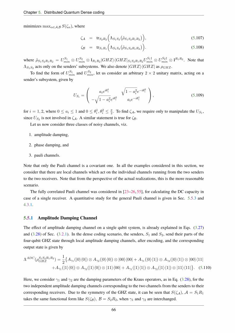
Chapter 5. Distributed Quantum Dense coding

minimizes max↵2A,B S(⇣↵), where

⇣A = trS2R2

⇣⇤S1S2

�⇢S1S2R1R2

�⌘, (5.107)

⇣B = trS1R1

⇣⇤S1S2

�⇢S1S2R1R2

�⌘. (5.108)

where ⇢S1S2R1R2 = US1min ⌦ U

S2min ⌦ IR1R2 |GHZihGHZ|S1S2R1R2U

S1†min ⌦ U

S2†min ⌦ IR1R2 . Note that

⇤S1S2 acts only on the senders’ subsystems. We also denote |GHZihGHZ| as ⇢GHZ .To find the form of US1

min and US2min, let us consider an arbitrary 2 ⇥ 2 unitary matrix, acting on a

sender’s subsystem, given by

USi=

0

@ aiei✓1

i

q1� a

2i e�i✓2

i

�

q1� a

2i e

i✓2i aie

�i✓1i

1

A , (5.109)

for i = 1, 2, where 0 ai 1 and 0 ✓1i , ✓

2i

⇡2 . To find ⇣A, we require only to manipulate the US1 ,

since US2 is not involved in ⇣A. A similar statement is true for ⇣B.Let us now consider three classes of noisy channels, viz.

1. amplitude damping,

2. phase damping, and

3. pauli channels.

Note that only the Pauli channel is a covariant one. In all the examples considered in this section, weconsider that there are local channels which act on the individual channels running from the two sendersto the two receivers. Note that from the perspective of the actual realizations, this is the more reasonablescenario.

The fully correlated Pauli channel was considered in [23–26, 55], for calculating the DC capacity incase of a single receiver. A quantitative study for the general Pauli channel is given in Sec. 5.5.3 and4.3.1.

5.5.1 Amplitude Damping Channel

The e�ect of amplitude damping channel on a single qubit system, is already explained in Eqs. (3.27)and (3.28) of Sec. (3.2.1). In the dense coding scenario, the senders, S1 and S2, send their parts of thefour-qubit GHZ state through local amplitude damping channels, after encoding, and the correspondingoutput state is given by

⇤ADC(⇢S1S2R1R2GHZ ) =

1

2

�A�1(|0ih0|)⌦A�2(|0ih0|)⌦ |00ih00|+A�1(|0ih1|)⌦A�2(|0ih1|)⌦ |00ih11|

+A�1(|1ih0|)⌦A�2(|1ih0|)⌦ |11ih00|+A�1(|1ih1|)⌦A�2(|1ih1|)⌦ |11ih11| . (5.110)

Here, we consider �1 and �2 are the damping parameters of the Kraus operators, as in Eq. (3.28), for thetwo independent amplitude damping channels corresponding to the two channels from the senders to theircorresponding receivers. Due to the symmetry of the GHZ state, it can be seen that S(⇣A), A = S1R1

takes the same functional form like S(⇣B), B = S2R2, when �1 and �2 are interchanged.

66

5.5. Examples of noisy quantum channels

Figure 5.3: Plots of the quantities a21pf(a1)

log1�p

f(a1)

1+p

f(a1)and 1�a21p

g(a1)log

1�p

g(a1)

1+p

g(a1), which are respectively

the left-hand- and right-hand-sides of Eq. (5.116), against a1 and �. The green (gray in print) surfacerepresents the first while the purple (dark in print) one is for the second expression. The intersection line(white line) is a1 = 1p

2, for all �. The base axes are dimensionless, while the vertical axis is in bits.

By using the unitary operator given in Eq. (5.109), one can find that the eigenvalues of ⇣A are

�1 =1

4

⇣1�

pf(a1)

⌘, (5.111)

�2 =1

4

⇣1 +

pf(a1)

⌘, (5.112)

�3 =1

4

⇣1�

pg(a1)

⌘, (5.113)

�4 =1

4

⇣1 +

pg(a1)

⌘, (5.114)

where f(a) = 1�4�1(1��1)a4 and g(a) = 1�4�1(1��1)(1�a2)2. Note that the �i’s are independent

of the ✓j1.

The minimization of S(⇣A) = �P

i �i log �i ⌘ F (a1), say, is obtained by calculating

dF (a1)

da1= 0, (5.115)

which lead to the relation given by

a21p

f(a1)log

1�pf(a1)

1 +pf(a1)

=1� a

21p

g(a1)log

1�pg(a1)

1 +pg(a1)

, (5.116)

Solutions of the above equation give the extrema. In Fig. 5.3, we plot the L.H.S (left-hand-side, greensurface) and R.H.S (purple surface) of Eq. (5.116). The intersection line, a1 = 1p

2, of these two surfaces

67

Chapter 5. Distributed Quantum Dense coding

gives the solution of Eq. (5.116).To check whether it is minimum or not, we find

d2F (a1)

da21

����a1=

1p2

= ��(1� �)p

(1� � + �2)3

log

1�

p1� � + �2

1 +p1� � + �2

!⇥ 4 + 8

p1� � + �2

�, (5.117)

which is non-negative for all �, at a1 = 1p2, confirming the minimum. Therefore, the minimum

of S(⇣A) is obtained at a1 = 1p2

and is given by 1 + H(12(1 �p

1� �1 + �21)), where h(x) =

�x log x� (1�x) log(1�x) is the Shannon binary entropy given in Eq. (2.14). Similarly, one can obtainthe minimum of S(⇣B). Note that there is a single extremal point obtained and the corresponding functionis continuous, which implies that the local minimum obtained here is actually the global minimum.Therefore, for the amplitude damping channel, if the input state is the GHZ state, then the upper boundon the LOCC-DC capacity is given by

BLOCCADC = 3� max

x21,2h

✓1

2(1�

p1� �x + �2x)

◆. (5.118)

Note that in a noiseless scenario, CLOCC = 3 = BLOCC for the shared GHZ state.

5.5.2 Phase Damping Channel

Phase damping channel, ⇤PD, transformed the state ⇢, as

⇤PD(⇢) = M0⇢M†0 +M1⇢M

†1 +M2⇢M

†2 , (5.119)

where the Mi’s are the Kraus operators given in Eq. (3.31), Here we again assume that the noise is localon the senders’ parts. In this case, the eigenvalues of ⇣A are given by

�1 = �2 =1

4

⇣1�

pfP (a1)

⌘, (5.120)

�3 = �4 =1

4

⇣1 +

pfP (a1)

⌘, (5.121)

where fP (a) = 1 � 4a2(1 � a2)p(2 � p). Like in the case of the amplitude damping channel, the

minimization does not depend on the ✓i’s. It is also clear from the concavity of the von Neumann entropythat maximizing fP (a1) is enough to minimize S(⇣1). Note that when fP (a1) increases, �1 and �2 goclose to zero while �3 and �4 tend to 0.5, which in turn minimize S(⇣A). The second term in fP (a1) isa positive quantity, the maximum value of fP (a1) is 1, when a = 0 or 1, and hence we have S(⇣1) = 1.Therefore, for the phase damping channel, we get

BLOCCPD = 3, (5.122)

which is independent of the parameters of the channel.

5.5.3 Pauli Noise: A Covariant Channel

Pauli noise is an example of a covariant noise, which satisfies the covariant condition, given in Eq.(3.41). When an arbitrary qubit state, is passed through the channel with Pauli noise [59,178], the state is

68

5.5. Examples of noisy quantum channels

transformed as

⇤P (⇢) =3X

m=0

qm�m⇢�m (5.123)

where {�m} are the well-known Pauli spin matrices along with the identity operators, i.e,

�1 = �x =

0 1

1 0

!, �2 = �y =

0 �i

i 0

!,

�3 = �z =

1 0

0 �1

!, �0 = I =

1 0

0 1

!.

Consider a four-qubit state, ⇢S1S2R1R2 , shared between two senders and two receivers. After passingthrough the Pauli channel, it transforms as

⇤PS1S2R1R2

(⇢S1S2R1R2) =3X

m,n=0

qmn��S1m ⌦ �

S2n ⌦ IR1R2

�⇢S1S2R1R2

��S1m ⌦ �

S2n ⌦ IR1R2

�, (5.124)

whereP

mn qmn = 1. Depending on the choice of qmn, the channel can be correlated (see Sec. 4.3.1) oruncorrelated (see Sec. 4.3.2) . We deal with the fully-correlated Pauli channel, i.e, when qmn = qm�mn.Eq. (5.124) in this case reduces to

⇤fPS1S2R1R2

(⇢S1S2R1R2) =3X

m=0

qm��S1m ⌦ �

S2m ⌦ IR1R2

�⇢S1S2R1R2

��S1m ⌦ �

S2m ⌦ IR1R2

�. (5.125)

Let us find out the Umin for the four-qubit GHZ state shared between two senders and two receivers, inthe presence of the fully-correlated Pauli noise as in Eq. (5.125). From the symmetry of the GHZ state,we have S(⇣A) = S(⇣B). The eigenvalues of ⇣A are given by

�1 = �2 =1

4

✓1�

qg(a1, ✓11, ✓

21)

◆, (5.126)

�3 = �4 =1

4

✓1 +

qg(a1, ✓11, ✓

21)

◆, (5.127)

where

g(a, ✓) ⌘ g(a, ✓1, ✓2) = (q0 � q1 � q2 + q3)2 + f1(a)[8q1q2 + 8q0q3 � 4(q0 + q3)(q1 + q2)

�4(q1 � q2)(q0 � q3) cos(2(✓1 + ✓2))] (5.128)

and f1(a) = 2a2(�1 + a2). Arguing in the same way as in other cases, it is enough to maximize g(a, ✓),

with ✓ = ✓1 + ✓2, in order to minimize S(⇣A). To find the extremum of g(a, ✓), we have to solve

@g(a, ✓)

@a= 0, (5.129)

and@g(a, ✓)

@✓= 0, (5.130)

69

Chapter 5. Distributed Quantum Dense coding

which give the extremum value at a = a0 ⌘ 0 or 1p2, and ✓ = ✓0 ⌘

n⇡2 , where n 2 Z. g(a, ✓) is a

function of the noise parameters {qm}, and to find the extremum, without loss of generality, we assumean ordering of those parameters, i.e., we assume

q0 � q2 � q1 � q3. (5.131)

And g(a, ✓) is maximum, when

@2g(a, ✓)

@a2

����a0,✓0

,@2g(a, ✓)

@✓2

����a0,✓0

< 0, (5.132)

✓@2g

@a@✓

◆2�����a0,✓0

<@2g

@a2

@2g

@✓2

����a0,✓0

, (5.133)

are satisfied simultaneously. For the above choice of qm, the maximum value ofpg(a, ✓) is |q0 � q1 +

q2 � q3|, which will be achieved, when a = 1p2

and ✓ is odd multiple of ⇡2 , S(⇣A) = q(q0 + q2) + 1, andU

S1min is given by

US1min =

1p2

ei✓11 �ie

i✓11

�ie�i✓11 e

�i✓11

!.

If we take another ordering of {qm}, for e.g., q1 � q2 � q0 � q3, we have S(⇣1) = H(q1 + q2) + 1, andthe unitary operator, in this case, is given by

US1min =

0 e

i✓11

e�i✓11 0

!.

The above two cases indicate that the minimum entropy depends on the ordering of qm, involved in thechannel with Pauli noise. In general, when the shared state is the GHZ state, the capacity �LOCC

Pauli isbounded above by 3� h(b1 + b2), where {bm}

4m=1, is an arrangement of {qm} in descending order.

Instead of fully correlated Pauli noise, if we now assume that the qmn is arbitrary, the strategy of fullycorrelated Pauli noise can also be applied in this case. Suppose, pm =

Pn qmn and rn =

Pm qmn. Then

the capacity is bounded above as

�LOCCPauli = 3�max{h(b1 + b2), h(c1 + c2)}, (5.134)

where {bm}4m=1 and {cn}

4n=1 are the sets {pm} and {rn} in descending order.

5.6 Connecting Multipartite Entanglement with LOCC-DC

In this section, we establish a relation between the capacities of LOCC-DC of four-qubit pure states withtwo senders and two receivers and their genuine multiparty entanglement content in terms of GGM (E).The protocol considered here is due to collective involvement/contribution of all the parties involved, i.e.,senders and receivers. This led us to establish a connection between the capacity of such dense codingprotocol to a genuine multiparty entanglement present in the system. Specifically, we will estimate theordering of the GGMs between the generalized GHZ state and an arbitrary four-qubit pure state, when both

70

5.6. Connecting Multipartite Entanglement with LOCC-DC

of them have equal LOCC dense coding capacities. Such estimation will shed light on the bridge betweenmultiparty entanglement as quantified by the generalized geometric measure and multiport capacity asquantified by the LOCC-DC capacity.

Note that although the exact capacity of dense coding by LOCC for arbitrary multiparty pure state isnot known, it was shown [21, 22] that the exact capacity is 3 for the four-qubit GHZ state, given in Eq.(5.73). In case of the gGHZ state, shared between two senders and two receivers, given in Eq. (4.1), is

|gGHZiS1S2R1R2 = (p↵|0000i+

p1� ↵2e

i�|1111i)S1S2R1R2 , (5.135)

the capacity of LOCC-DC is bounded above by

BLOCC(|gGHZi) = 2 + h(↵). (5.136)

From the intuition obtained from bipartite non-maximally entangled states, we conjecture here that thecapacity of LOCC-DC for the gGHZ state saturates the upper bound, BLOCC . With this assumption, wehave the following result.Result: Consider a multiparty DC protocol where there are two senders and two receivers, and wherethe channels from the senders to the receivers are noiseless. In this case if a four-qubit gGHZ state andan arbitrary four-qubit pure state have equal capacities of LOCC-DC, then the gGHZ state possesses lessgenuine multiparty entanglement than that of the arbitrary state i.e, we have

E(| i) � E(|gGHZi), (5.137)

if (i) S(⇢R1) S(⇢S1R1), i.e., the reduced state, ⇢S1R1 , has more disorder than its local subsystem, ⇢R1 ,and (ii) the maximum eigenvalue required for GGM is obtained from the density matrix, ⇢R2 . Similarconditions can be obtained by interchanging S1 and R1 with S2 and R2 respectively.Proof: As argued above, it is plausible that for the gGHZ state,

CLOCCgGHZ = 2 + h(↵). (5.138)

For an arbitrary four-qubit pure state, | i, shared between the senders S1, S2 and receivers R1, R2, theupper bound of the capacity of LOCC-DC is given by

CLOCC B

LOCC(| i) = 2 + S(⇢R1) + S(⇢R2)� S(⇢S1R1), (5.139)

where S(⇢Ri), i = 1, 2, and S(⇢S1R1) are the reduced density matrices of | i.

Note that for pure state S(⇢S1R1) = S(⇢S2R2). Let us now assume that the LOCC-DC capacities for| i and the gGHZ state are equal, so that

CLOCCgGHZ = 2 + h(↵) = C

LOCC

2 + S(⇢R1) + S(⇢R2)� S(⇢S1R1), (5.140)

which implies h(↵) S(⇢R2), provided S(⇢R1) S(⇢S1R1). This implies that

↵ � �R2 , (5.141)

71

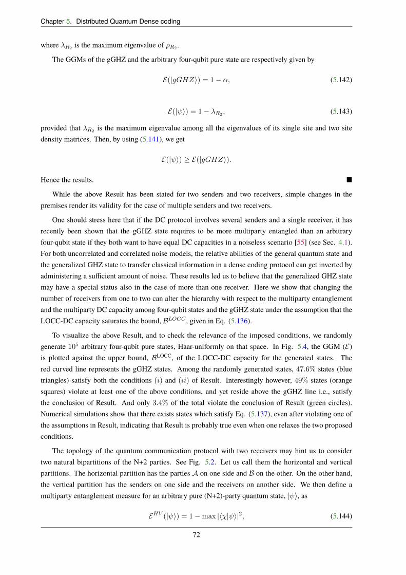
Chapter 5. Distributed Quantum Dense coding

where �R2 is the maximum eigenvalue of ⇢R2 .

The GGMs of the gGHZ and the arbitrary four-qubit pure state are respectively given by

E(|gGHZi) = 1� ↵, (5.142)

E(| i) = 1� �R2 , (5.143)

provided that �R2 is the maximum eigenvalue among all the eigenvalues of its single site and two sitedensity matrices. Then, by using (5.141), we get

E(| i) � E(|gGHZi).

Hence the results. ⌅

While the above Result has been stated for two senders and two receivers, simple changes in thepremises render its validity for the case of multiple senders and two receivers.

One should stress here that if the DC protocol involves several senders and a single receiver, it hasrecently been shown that the gGHZ state requires to be more multiparty entangled than an arbitraryfour-qubit state if they both want to have equal DC capacities in a noiseless scenario [55] (see Sec. 4.1).For both uncorrelated and correlated noise models, the relative abilities of the general quantum state andthe generalized GHZ state to transfer classical information in a dense coding protocol can get inverted byadministering a su�cient amount of noise. These results led us to believe that the generalized GHZ statemay have a special status also in the case of more than one receiver. Here we show that changing thenumber of receivers from one to two can alter the hierarchy with respect to the multiparty entanglementand the multiparty DC capacity among four-qubit states and the gGHZ state under the assumption that theLOCC-DC capacity saturates the bound, BLOCC , given in Eq. (5.136).

To visualize the above Result, and to check the relevance of the imposed conditions, we randomlygenerate 105 arbitrary four-qubit pure states, Haar-uniformly on that space. In Fig. 5.4, the GGM (E)is plotted against the upper bound, BLOCC, of the LOCC-DC capacity for the generated states. Thered curved line represents the gGHZ states. Among the randomly generated states, 47.6% states (bluetriangles) satisfy both the conditions (i) and (ii) of Result. Interestingly however, 49% states (orangesquares) violate at least one of the above conditions, and yet reside above the gGHZ line i.e., satisfythe conclusion of Result. And only 3.4% of the total violate the conclusion of Result (green circles).Numerical simulations show that there exists states which satisfy Eq. (5.137), even after violating one ofthe assumptions in Result, indicating that Result is probably true even when one relaxes the two proposedconditions.

The topology of the quantum communication protocol with two receivers may hint us to considertwo natural bipartitions of the N+2 parties. See Fig. 5.2. Let us call them the horizontal and verticalpartitions. The horizontal partition has the parties A on one side and B on the other. On the other hand,the vertical partition has the senders on one side and the receivers on another side. We then define amultiparty entanglement measure for an arbitrary pure (N+2)-party quantum state, | i, as

EHV (| i) = 1�max |h�| i|2, (5.144)

72

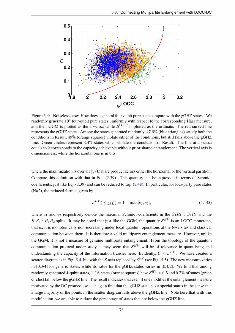
5.6. Connecting Multipartite Entanglement with LOCC-DC

0

0.1

0.2

0.3

0.4

0.5

1.8 2 2.2 2.4 2.6 2.8 3 3.2

ε

BLOCC

Figure 5.4: Noiseless case: How does a general four-qubit pure state compare with the gGHZ states? Werandomly generate 105 four-qubit pure states uniformly with respect to the corresponding Haar measure,and their GGM is plotted as the abscissa while B

LOCC is plotted as the ordinate. The red curved linerepresents the gGHZ states. Among the states generated randomly, 47.6% (blue triangles) satisfy both theconditions in Result, 49% (orange squares) violate either of the conditions, but still falls above the gGHZline. Green circles represent 3.4% states which violate the conclusion of Result. The line at abscissaequals to 2 corresponds to the capacity achievable without prior shared entanglement. The vertical axis isdimensionless, while the horizontal one is in bits.

where the maximization is over all |�i that are product across either the horizontal or the vertical partition.Compare this definition with that in Eq. (2.39). This quantity can be expressed in terms of Schmidtcoe�cients, just like Eq. (2.39) and can be reduced to Eq. (2.48). In particular, for four-party pure states(N=2), the reduced form is given by

EHV (| 1234i) = 1�max[e1, e2], (5.145)

where e1 and e2 respectively denote the maximal Schmidt coe�cients in the S1R1 : S2R2 and theS1S2 : R1R2 splits. It may be noted that just like the GGM, the quantity E

HV is an LOCC monotone,that is, it is monotonically non-increasing under local quantum operations at the N+2 sites and classicalcommunication between them. It is therefore a valid multiparty entanglement measure. However, unlikethe GGM, it is not a measure of genuine multiparty entanglement. From the topology of the quantumcommunication protocol under study, it may seem that EHV will be of relevance in quantifying andunderstanding the capacity of the information transfer here. Evidently, E E

HV . We have created ascatter diagram as in Fig. 5.4, but with the E axis replaced by E

HV (see Fig. 5.5). The new measure variesin [0,3/4] for generic states, while its value for the gGHZ states varies in [0,1/2]. We find that amongrandomly generated 4-qubit states, 1.2% states (orange squares) have EHV

> 0.5 and 0.7% of states (greencircles) fall below the gGHZ line. The result indicates that even if one modifies the entanglement measuremotivated by the DC protocol, we can again find that the gGHZ state has a special status in the sense thata large majority of the points in the scatter diagram falls above the gGHZ line. Note here that with thismodification, we are able to reduce the percentage of states that are below the gGHZ line.

73

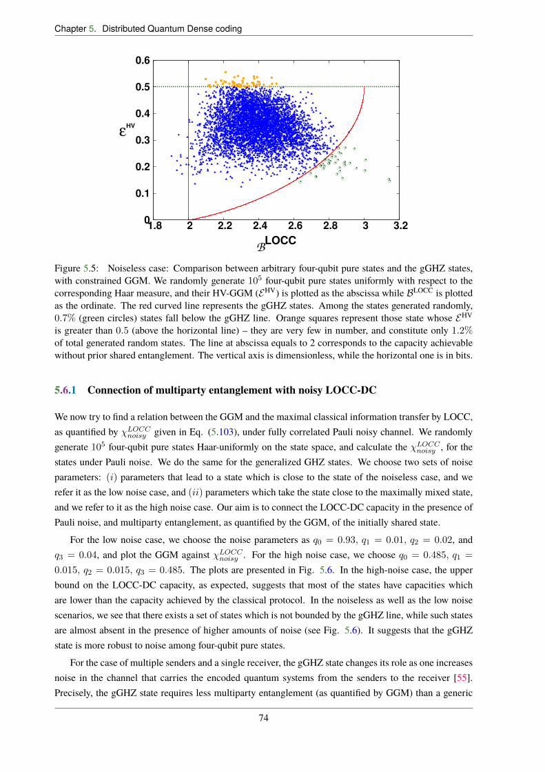
Chapter 5. Distributed Quantum Dense coding

0

0.1

0.2

0.3

0.4

0.5

0.6

1.8 2 2.2 2.4 2.6 2.8 3 3.2

εHV

BLOCC

Figure 5.5: Noiseless case: Comparison between arbitrary four-qubit pure states and the gGHZ states,with constrained GGM. We randomly generate 105 four-qubit pure states uniformly with respect to thecorresponding Haar measure, and their HV-GGM (EHV) is plotted as the abscissa while BLOCC is plottedas the ordinate. The red curved line represents the gGHZ states. Among the states generated randomly,0.7% (green circles) states fall below the gGHZ line. Orange squares represent those state whose E

HV

is greater than 0.5 (above the horizontal line) – they are very few in number, and constitute only 1.2%of total generated random states. The line at abscissa equals to 2 corresponds to the capacity achievablewithout prior shared entanglement. The vertical axis is dimensionless, while the horizontal one is in bits.

5.6.1 Connection of multiparty entanglement with noisy LOCC-DC

We now try to find a relation between the GGM and the maximal classical information transfer by LOCC,as quantified by �LOCC

noisy given in Eq. (5.103), under fully correlated Pauli noisy channel. We randomlygenerate 105 four-qubit pure states Haar-uniformly on the state space, and calculate the �LOCC

noisy , for thestates under Pauli noise. We do the same for the generalized GHZ states. We choose two sets of noiseparameters: (i) parameters that lead to a state which is close to the state of the noiseless case, and werefer it as the low noise case, and (ii) parameters which take the state close to the maximally mixed state,and we refer to it as the high noise case. Our aim is to connect the LOCC-DC capacity in the presence ofPauli noise, and multiparty entanglement, as quantified by the GGM, of the initially shared state.

For the low noise case, we choose the noise parameters as q0 = 0.93, q1 = 0.01, q2 = 0.02, andq3 = 0.04, and plot the GGM against �LOCC

noisy . For the high noise case, we choose q0 = 0.485, q1 =

0.015, q2 = 0.015, q3 = 0.485. The plots are presented in Fig. 5.6. In the high-noise case, the upperbound on the LOCC-DC capacity, as expected, suggests that most of the states have capacities whichare lower than the capacity achieved by the classical protocol. In the noiseless as well as the low noisescenarios, we see that there exists a set of states which is not bounded by the gGHZ line, while such statesare almost absent in the presence of higher amounts of noise (see Fig. 5.6). It suggests that the gGHZstate is more robust to noise among four-qubit pure states.

For the case of multiple senders and a single receiver, the gGHZ state changes its role as one increasesnoise in the channel that carries the encoded quantum systems from the senders to the receiver [55].Precisely, the gGHZ state requires less multiparty entanglement (as quantified by GGM) than a generic

74

5.7. In closing

0

0.1

0.2

0.3

0.4

0.5

1.8 2 2.2 2.4 2.6 2.8 3

ε

χLOCC

noisy

0

0.1

0.2

0.3

0.4

0.5

1.8 2 2.2 2.4 2.6 2.8 3

ε

χLOCC

noisy

(a) (b)

Figure 5.6: Fully correlated Pauli noise: The gGHZ states are again better than a significant fraction ofstates. We plot the GGM as the ordinate and �LOCC

noisy as the abscissa for 105 randomly generated four-qubitpure states uniformly with respect to the corresponding Haar measure for low (figure (a)) and high (figure(b)) full correlated Pauli noise. In figure (a), q0 = 0.93, q1 = 0.01, q2 = 0.02, q3 = 0.04, while in figure(b), we choose q0 = 0.485, q1 = 0.015, q2 = 0.015, q3 = 0.485. In the presence of high noise, almost allstates are bounded by the four-qubit gGHZ states (red curved line). A significant fraction of the generatedstates lie above the gGHZ line even for low noise. It indicates that the gGHZ state is more robust againstnoise as compared to an arbitrary four-qubit pure state. The lines at abscissa equals to 2 correspond tothe capacity achievable without prior shared entanglement. The vertical axis is dimensionless, while thehorizontal one is in bits.

state to be equal in dense coding capacity with the generic state, if the channels are noisy. The opposite istrue when the channels are noiseless. Here we see that if there are two receivers in the protocol, there is nosuch role reversal. The gGHZ state requires less multiparty entanglement than a generic state to have thesame LOCC dense coding capacity as the generic state. Note that this statement in under the assumptionthat the upper bounds on the LOCC-DC capacities faithfully mirror the qualitative features of the actualcapacities.

5.7 In closing

The dense coding protocol is a quantum communication scheme which demonstrates that the classicalinformation can be transferred via quantum states more e�ciently than any classical protocol. The“Holevo bound” is applied to obtain the capacities, when there is a single sender and a single receiver aswell as when there are multiple senders and a single receiver. Capacities are known for both noiselessand for certain noisy channels. However, realistic scenarios of a communication protocol should involvemultiple senders and multiple receivers, when the receivers can not make any global quantum operations.The di�culty in such generalization is due to the nonexistence, hitherto, of a Holevo-like bound in themultipartite decoding process in the many-receivers scenario in the case of noisy channels. In this chapter,we discuss the problem in getting the distributed dense coding capacity or LOCC-DC capacity involvingmultiple senders and two receivers, and observe that there is an upper bound on the LOCC-DC which isachievable for four-qubit GHZ state. We address the problem of estimating the dense coding capacity,in the same situation when the transmission channel used by the senders to send their encoded part tothe receivers is noisy. In particular, we find an upper bound on the classical capacity of the multipartite

75

Chapter 5. Distributed Quantum Dense coding

quantum channel, when the senders and receivers share a multiparty quantum state and noisy channels,and the receivers are allowed to perform only local quantum operations and classical communication. Acompact form of the upper bound on the capacity is obtained when the noisy channels are covariant. Whenthe four-party shared state is the GHZ state, several paradigmatic noisy channels are considered and theupper bounds on the capacities are determined. Finally, we connect the capacity of dense coding with amultiparty entanglement measure, both in the noiseless and noisy scenarios.

The results of this Chapter are based on the following paper:

1. Distributed quantum dense coding with two receivers in noisy environments, Tamoghna Das, R.Prabhu, Aditi Sen De, Ujjwal Sen, Phys. Rev. A 92, 052330 (2015).

76

Chapter 6Photon Subtracted State is MoreEntangled than Photon Added State

In the earlier chapters, we have talked about the quantum communication protocol involving several sendersand single as well as two receivers in both noiseless and noisy scenarios with the help of shared quantumstate. We connect the multiparty entanglement of the shared state with multiparty DC capacity andLOCC-DC capacity for noiseless and noisy scenarios and found that entanglement content of the sharedstate plays an important role in realizing those protocols. But to realize this quantum communicationprotocol in the laboratory for finite dimensional system, for example, in the qubit systems, there existssome di�culties [32–35].

One of the physical systems in which quantum information tasks have been realized in the laboratoryis the class of continuous variable (CV) systems. Historically, the notion of the quantum correlatedstate of two particles in CV systems first arrived in the seminal paper of Einstein, Podolosky, and Rosenin 1935 [62]. In recent years, several communications schemes like teleportation [5] and classicalinformation transfer by quantum channels [4], have extensively been investigated both theoretically andexperimentally, in CV systems, especially in Gaussian states [36, 38, 39, 41, 60]. However, it has beendiscovered that there are several protocols which can not be implemented using Gaussian states withGaussian operations. Examples include entanglement distillation [42], measurement-based universalquantum computation [44], teleportation [46], and quantum error correction [48]. Non-Gaussian statesare increasingly being found to be important in several applications. They have also been realized in thelaboratory [49, 50].

An important method to make such states is by adding and subtracting photons, from the Gaussianstates. The multimode squeezed vacuum state [51–54] is good example of entangled Gaussian stateas its quasiprobability distribution, the Wigner function [186], is a Gaussian function of its quadraturevariables [187, 188]. Starting from an entangled two-mode squeezed vacuum (TMSV) state, whoseWigner function [186] is always positive, it was shown that photon addition can generate a negative dipof the Wigner function in the phase space [189] and hence can deviate from being a Gaussian state. Incase of the two-mode squeezed vacuum (TMSV) state as input state, both the entanglement and fidelity ofteleportation can be increased by adding and subtracting photons to (from) one or two modes [51–54]. Forsuch experiments, see [190–192]. Moreover, the entanglement content of the photon-added state obtained

77

Chapter 6. Photon Subtracted State is More Entangled than Photon Added State

from the TMSV state was shown to be always higher than that of the photon-subtracted state [51–54].Investigations of the squeezed vacuum state with respect to photon addition and subtraction are usually

restricted to the two-mode case, even though the importance of multimode CV system is unquestionable[193–203]. Moreover, it is believed that multimode entangled states can be a resource to build quantumcommunication network, both for transferring classical as well as quantum information between severalsenders and several receivers [202]. In this paper, we consider the four-mode squeezed vacuum (FMSV)state as input, and deGaussify it by adding and subtracting photons in di�erent modes.

We evaluate entanglement between di�erent modes in all possible bipartitions and compare the resultsof the photon-added state with the subtracted ones. We call a mode as “player” mode when we analysethe e�ect on entanglement, by varying the number of photons added or subtracted in that mode. Therecould be several such player modes. The remaining modes, in which either no photons or a fixed numberof photons are added or subtracted, are referred to as the “spectator” modes. At last, we will also analyzethe bipartite entanglement of the output two party state which can be obtained by discarding either twoplayer modes or two spectator modes, and study the distance-based measure of non-Gaussianity of theoutput four-mode state under the e�ect of photon addition and subtraction.

6.1 N-mode squeezed vacuum state

In this section, we discuss the N-mode squeezed vacuum state (NMSV), specifically the two-mode andfour-mode squeezed vacuum states, and a state obtained after adding (subtracting) an arbitrary number ofphotons at the ith mode. These states are examples of entangled states in continuous variables which canbe used in various quantum information tasks. To define such states, let us first denote the bosonic creationand annihilation operators at the mode i, as a†i and ai respectively, which satisfy the bosonic commutationrelations, [ai, a†j ] = �ij , and [ai, aj ] = 0, [a†i , a

†j ] = 0. By using bosonic operators, an N -mode squeezed

vacuum state is given by| N i = S(✏)|0102 . . . 0N i, (6.1)

where |0102 . . . 0N i is the N-mode vacuum state and S(✏) is squeezing operator, which is defined as

S(✏) = exp

1

2

NX

i=1

⇣✏⇤aiai+1 � ✏a

†i a

†i+1

⌘!, (6.2)

where aN+1 = a1 and ✏ = rei✓ is the squeezing parameter. The above state in Eq. (6.1) is called a

squeezed state. To show that, let us consider the variances of N -mode quadrature operators �X1, and�X2, given by

�X1 =qhX

21 i � hX1i

2, (6.3)

�X2 =qhX

21 i � hX2i

2, (6.4)

where

X1 =X

j

qj =1

2pN

NX

j=1

(a†j + aj), (6.5)

78

6.1. N-mode squeezed vacuum state

X2 =X

j

pj =1

2pN

NX

j=1

�i(a†j � aj), (6.6)

with the position and momentum operators for each mode being

qj = (a†j + aj), (6.7)

pj = �i(a†j � aj). (6.8)

Here the average is taken over the NMSV state. To obtain the variances of �X1 and �X2, we need toobtain the following relations:

S(✏)†X

j

ajS(✏) = e

⇣� 1

2

PN

i=1

⇣✏⇤aiai+1�✏a†i a

†i+1

⌘⌘ NX

j=1

aje

⇣12

PN

i=1

⇣✏⇤aiai+1�✏a†i a

†i+1

⌘⌘

=NX

j=1

aj � ✏a†j +

|✏|2

2!aj �

✏|✏|2

3!a†j + · · ·

=NX

j=1

aj cosh r � ei✓a†j sinh r, (6.9)

where we use the Baker-Campbell-Hausdor� formula of any two operators A and B, given by

e�A

BeA = B �

⇥A, B

⇤+

1

2!

⇥A,

⇥A, B

⇤⇤�

1

3!

⇥A,

⇥A,

⇥A, B

⇤⇤⇤+ · · · . (6.10)

Similarly, we have

S(✏)†NX

j=1

a†jS(✏) =

NX

j=1

a†j cosh r � e

�i✓aj sinh r. (6.11)

Now putting these expressions in the expectation values of X21 and X1, we have,

hX21 i =

1

4Nh0102 . . . 0N |S(✏)†

⇣ NX

j=1

(a†j + aj)⌘2

S(✏)|0102 . . . 0N i,

=1

4Nh0102 . . . 0N |

NX

jk

⇣aj a

†k + a

†kaj

⌘|0102 . . . 0N i| cosh r � e

i✓ sinh r|2,

=1

4

✓e2r sin2

✓

2+ e�2r cos2

✓

2

◆, (6.12)

and

hX1i =1

2pNh0102 . . . 0N |S(✏)†

NX

j=1

(a†j + aj)S(✏)|0102 . . . 0N i = 0. (6.13)

We finally get

�X21 =

1

4

✓e2r sin2

✓

2+ e�2r cos2

✓

2

◆. (6.14)

79

Chapter 6. Photon Subtracted State is More Entangled than Photon Added State

Similarly, we have

�X22 =

1

4

✓e�2r sin2

✓

2+ e

2r cos2✓

2

◆. (6.15)

Thus for ✓ = 0 or ⇡, we have �X1�X2 = 14 . However, for any one of the i = 1, 2, �X1 = 1

2e�r

12 ,

while �X2 = 12e

r�

12 and vice-versa. This guarantees that the state, given in Eq. (6.1) is a squeezed

state. We assume ✓ = 0 throughout this chapter.

6.1.1 Another form of NMSV state

In this section, we will try to find out another form of the NMSV state, so that we can express the NMSVstate in terms of the photon number states or in the Fock number basis |nji of the jth mode, where

aj |nji =pnj |nj � 1i, (6.16)

a†j |nji =

pnj + 1|nj + 1i. (6.17)

To do this, we need some tools. Let us first calculate

S(r)†ajS(r) = aj �

h 12

NX

i=1

⇣raiai+1 � ra

†i a

†i+1

⌘

| {z }A

, aj

i+

1

2!

⇥A,

⇥A, aj

⇤⇤�

1

3!

⇥A,

⇥A,

⇥A, aj

⇤⇤⇤+ · · ·

= aj � r

NX

k=1

Qjka†k +

1

2!r2

NX

k=1

Q2jkak �

1

3!r3

NX

k=1

Q3jka

†k + · · · , (6.18)

=⇣I +

1

2!r2Q

2 +1

4!r4Q

4 + · · ·

⌘

jkak �

⇣rQ+

1

3!r3Q

3 + · · ·

⌘

jka†k (6.19)

=NX

k=1

cosh(rQ)jkak � sinh(rQ)jka†k, (6.20)

where the matrix Q can be obtained from the commutation relations

hA, aj

i= r

1

2

�a†j+1 + a

†j�1

�= r

NX

k=1

Qjka†k, 8j, (6.21)

⇥A,

⇥A, aj

⇤⇤= r

NX

k=1

Qjk

⇥A, a

†k

i= r

2NX

k,l=1

QjkQklal = r2

NX

k=1

Q2jkak, (6.22)

which is given by Qjk = 12(�j+1,k + �j�1,k). Similar relations, like Eq. (6.20), can also be obtained

which are given by

S(r)†a†jS(r) =NX

k=1

cosh(rQ)jka†k � sinh(rQ)jkak, (6.23)

S(r)ajS(r)† =

NX

k=1

cosh(rQ)jkak + sinh(rQ)jka†k, (6.24)

80

6.1. N-mode squeezed vacuum state

S(r)a†jS(r)† =

NX

k=1

cosh(rQ)jka†k + sinh(rQ)jkak. (6.25)

Now we apply an annihilation operator on the jth site of the NMSV state, and the resulting output state is

aj | N i = ajS(r)|0102 . . . 0N i = S(r)S(r)†ajS(r)|0102 . . . 0N i

= S(r)NX

k=1

�cosh(rQ)jkak � sinh(rQ)jka

†k

�|0102 . . . 0N i

= �

NX

k=1

sinh(rQ)jk S(r)a†kS(r)†S(r)|0102 . . . 0N i

= �

NX

k=1

sinh(rQ)jk⇣ NX

l=1

cosh(rQ)kla†l + sinh(rQ)klal

⌘| N i

= �

NX

k=1

⇣sinh(rQ) cosh(rQ)jka

†k + sinh2(rQ)jkak

⌘| N i. (6.26)

To get the second line, we use S(r)S(r)† = I and Eq. (6.20) while in the third line, we use the factthat ak|0102 . . . 0N i = 0. The forth line is obtained by using Eq. (6.25). After a little manipulation, werewrite Eq. (6.26) as

NX

k=1

�I + sinh2(rQ)

�jkak| N i = �

NX

k=1

sinh(rQ) cosh(rQ)jka†k| N i (6.27)

)

NX

k=1

cosh2(rQ)jkak| N i = �NX

k=1

�sinh(rQ) cosh(rQ)

�jka†k| N i (6.28)

) aj | N i = �NX

k=1

tanh(rQ)jka†k| N i, 8j. (6.29)

Since the matrix, Q, is symmetric it is diagonalizable, and hence the hyperbolic relations also hold for it.Now Eq. (6.29) can be compared to a di�erential equation, given by

df

dx= �k(x)f ) f = Ae

�Rk(x)dx

. (6.30)

By taking insight from the above solution, we forcefully write the solution of Eq. (6.29) as

| N i = A exp⇣�

1

2

NX

jk=1

tanh(rQ)jka†j a

†k

⌘|0102 . . . 0N i, (6.31)

where A is the normalization constant. Now we will check that the above form of | N i is indeed thesolution of Eq. (6.29), by considering

al| N i = A

1X

n

1

n!al

⇣�

1

2

NX

jk=1

tanh(rQ)jka†j a

†k

⌘n|0102 . . . 0N i, (6.32)

81

Chapter 6. Photon Subtracted State is More Entangled than Photon Added State

and by observing

al

⇣�

1

2

NX

jk=1

tanh(rQ)jka†j a

†k

⌘n= �n

NX

m=1

tanh(rQ)lma†m

⇣�

1

2

NX

jk=1

tanh(rQ)jka†j a

†k

⌘n�1

+⇣�

1

2

NX

jk=1

tanh(rQ)jka†j a

†k

⌘nal. (6.33)

By putting Eq. (6.33) in Eq. (6.32), we obtain

al| N i = �A

1X

n

1

n!n

NX

m=1

tanh(rQ)lma†m

⇣�

1

2

NX

jk=1

tanh(rQ)jka†j a

†k

⌘n�1|0102 . . . 0N i

= �

NX

m=1

tanh(rQ)lma†m

✓A

1X

n

1

(n� 1)!

⇣�

1

2

NX

jk=1

tanh(rQ)jka†j a

†k

⌘n�1◆

|0102 . . . 0N i

= �

NX

m=1

tanh(rQ)lma†mA exp

⇣�

1

2

NX

jk=1

tanh(rQ)jka†j a

†k

⌘|0102 . . . 0N i

= �

NX

k=1

tanh(rQ)lka†k| N i. (6.34)

6.1.2 Two-mode squeezed vacuum state

The two-mode squeezed vacuum state (TMSV) can be obtained by putting N = 2 in Eq. (6.31), with

Q =

0 1

1 0

!, (6.35)

and

tanh rQ =

0 tanh r

tanh r 0

!. (6.36)

The normalization constant A = 1cosh r and hence, the TMSV state, with r as the squeezing parameter, is

given by

| 2i =1

cosh re� tanh ra†1a

†2 |00i (6.37)

=1

cosh r

1X

n=0

1

n!

�� tanh ra†1a

†2

�n|00i

=1

cosh r

1X

n=0

(� tanh r)n|ni|ni, (6.38)

where |ni = (a†)npn|0i is the occupation number state. Taking | 2i as the initial state, the behavior of

entanglement and non-Gaussianity, after adding or subtracting photons, have extensively been investigated[51–54] in last few years.

82

6.2. Preparation of FMSV state

6.1.3 Four-mode squeezed vacuum state

Let us now consider the four mode squeezed vacuum state, (FMSV) which can be obtained by settingN = 4 in Eq. (6.31). The 4⇥ 4 matrix, Q, in this case, takes the form

Q =1

2

0

BBBB@

0 1 0 1

1 0 1 0

0 1 0 1

1 0 1 0

1

CCCCA, (6.39)

and

tanh(rQ) =1

2tanh r

0

BBBB@

0 1 0 1

1 0 1 0

0 1 0 1

1 0 1 0

1

CCCCA, (6.40)

with A = 1cosh r . The FMSV state, then reads as [198,204, 205]

| 4i =1

cosh rexp

⇣�

1

2tanh r

�a†1 + a

†3

��a†2 + a

†4

�⌘|0000i. (6.41)

Expanding the exponential in Eq. (6.41), we have

| 4i =1

cosh r

1X

n=0

✓�1

2tanh r

◆n nX

r1,r2=0

s✓n

r1

◆✓n

r2

◆|n� r1i|n� r2i|r1i|r2i. (6.42)

Such an FMSV state can be prepared in the laboratory by using currently available technology [198]. Inthe next section, we will elaborate how one can prepare the FMSV state in the laboratory.

6.2 Preparation of FMSV state

To prepare [198] the FMSV state, we need two single mode squeezed vacuum (SMSV) states, with thesame squeezing parameter r. Moreover, if for one mode, the variance of quadrature operator X1 issqueezed to �X1 = 1

2e�r, then for the other one the opposite quadrature operator will be squeezed i.e.,

�X2 =12e�r. The two SMSV states are given by

|ri1 = exp⇣r

2

�a21 � a

†21

�⌘|0i =

1pcosh r

exp⇣� tanh r

a†21

2

⌘|0i, (6.43)

|� ri2 = exp⇣r

2

�a†22 � a

22

�⌘|0i =

1pcosh r

exp⇣tanh r

a†22

2

⌘|0i. (6.44)

These two SMSV states are sent through a 50 : 50 beam spliter, B12(⇡4 ), as shown in Fig. 6.1, where the

beam spliter [187, 188,198] is given by

B12(✓) = e�✓�a†1a2�a1a

†2

�. (6.45)

83

Chapter 6. Photon Subtracted State is More Entangled than Photon Added State

| − #⟩|#⟩1

2

%&'()4) 1

2 |-'⟩

|0⟩%'/(

)4)

24

|0⟩ 3

%&0()4)

3

1

|-/⟩

Figure 6.1: Schematic description of the preparation of FMSV state in the laboratory. Here |ri and |� ri

are two SMSV states with squeezing parameter r, squeezed di�erent quadrature operators. After passingthrough the 50 : 50 Beam splitter, it creats the TMSV state, | 2i, given in Eq. (6.37). Then the twomodes of TMSV state pass through the another 50 : 50 beam splitter along with the vacuums, resultingthe FMSV state as in Eq. (6.41).

The output state then reads as

B12�⇡4

�|ri1|� ri2 = B12

�⇡4

� 1

cosh rexp

⇣12tanh r

�a†22 � a

†21

�⌘B12

�⇡4

�†B12

�⇡4

�|00i, (6.46)

=1

cosh rexp

⇣B12

�⇡4

�12tanh r

�a†22 � a

†21

�B12

��⇡

4

�⌘|00i. (6.47)

The term in the exponential can be written as

e�A

BeA = B �

⇥A, B

⇤+

1

2!

⇥A,

⇥A, B

⇤⇤�

1

3!

⇥A,

⇥A,

⇥A, B

⇤⇤⇤+ · · · (6.48)

= �1

2tanh r

h�a†22 � a

†21

�+ ⇡a

†1a

†2 �

1

2!

⇡2

4

�a†22 � a

†21

��

1

3!

⇡3

4a†1a

†2 +

1

4!

⇡4

42�a†22 � a

†21

�

+1

5!

⇡5

42a†1a

†2 �

1

6!

⇡6

43�a†22 � a

†21

�+ · · ·

i(6.49)

= �1

2tanh r

h�a†22 � a

†21

�n1�

1

2!

�⇡2

�2+

1

4!

�⇡4

�4+ · · ·

o

| {z }cos

�⇡

2

�=0

+2a†1a†2

n�⇡2

��

1

3!

�⇡2

�3+

1

5!

�⇡2

�5· · ·

o

| {z }sin�

⇡

2

�=1

(6.50)

= � tanh ra†1a†2. (6.51)

84

6.3. Photon-added and -subtracted FMSV state

Here we put A = �⇡4

�a†1a2 � a1a

†2

�, and B = 1

2 tanh r�a†22 � a

†21

�. Putting Eq. (6.51) in Eq. (6.47),

we obtain the TMSV, given in Eq. (6.37). The FMSV state can then be obtained when each part of theTMSV state along with two vacuum states are sent through two di�erent 50 : 50 beam spliters (see Fig.(6.1)), i.e.,

B13�⇡4

�B24

�⇡4

�| 2i12|00i34 =

1

cosh rexp

⇣�B13

�⇡4

�B24

�⇡4

�tanh ra†1a

†2B13

��⇡

4

�B24

��⇡

4

�⌘|0000i.

(6.52)

Once again the term in the exponential can be written as e�ABeA, where

A =⇡

4

�a†1a3 � a1a

†3 + a

†2a4 � a2a

†4

�. (6.53)

and B = a†1a

†2. Similarly the individual terms in the right hand side of Eq. (6.10) as

⇥A, B

⇤= �

⇡

4

�a†2a

†3 + a

†1a

†4

�, (6.54)

⇥A,

⇥A, B

⇤⇤= �

⇡2

23�a†1a

†2 � a

†3a

†4

�, (6.55)

⇥A,

⇥A,

⇥A, B

⇤⇤⇤=⇡3

24(a†2a

†3 + a

†1a

†4

�. (6.56)

Putting the above equations in the exponential and using Eq. (6.10), we get

e�A

BeA = tanh r

na†1a

†2 +

⇡

4

�a†2a

†3 + a

†1a

†4

��

1

2!

⇡2

2 · 22�a†1a

†2 � a

†3a

†4

��

1

3!

⇡3

2 · 23�a†2a

†3 + a

†1a

†4

�

+1

4!

⇡4

2 · 24�a†1a

†2 � a

†3a

†4

�+

1

5!

⇡5

2 · 25�a†2a

†3 + a

†1a

†4

�o(6.57)

= tanh rh12

�a†1a

†2 + a

†3a

†4

�+

1

2

�a†1a

†2 � a

†3a

†4

�n1�

1

2!

�⇡2

�2+

1

4!

�⇡4

�4+ · · ·

o

+1

2

�a†2a

†3 + a

†1a

†4

�n�⇡2

��

1

3!

�⇡2

�3+

1

5!

�⇡2

�5· · ·

oi(6.58)

=1

2tanh r

�a†1a

†2 + a

†3a

†4 + a

†2a

†3 + a

†1a

†4

�

=1

2tanh r

�a†1 + a

†3

��a†2 + a

†4

�. (6.59)

Substituting the expression in the exponential of Eq. (6.52), we obtain Eq. (6.41) of the FMSV state | 4i.

6.3 Photon-added and -subtracted FMSV state

In this section, we consider the FMSV state, | 4i, as an initial state and our aim is to find the characteristicsof its entanglement after adding and subtracting a finite number of photons. For investigations, we useentanglement, according to the measures of entropy of entanglement and the logarithmic negativity,defined in Sec. 2.2.1 as measures of entanglement. Suppose mi number of photons are added at eachmode i, with i = 1, 2, 3, 4. Then the output four-mode (FM) state reads as

| add{mi}i =

1

Nadd

1X

n=0

✓�tanh r

2

◆n nX

r1,r2=0

s✓n

r1

◆✓n

r2

◆s(n� r1 +m1)!

(n� r1)!

s(n� r2 +m2)!

(n� r2)!

85

Chapter 6. Photon Subtracted State is More Entangled than Photon Added State

s(r1 +m3)!

r1!

s(r2 +m4)!

r2!⇥ |n� r1 +m1i|n� r2 +m2i|r1 +m3i|r2 +m4i

⌘

1X

n=0

nX

r1,r2=0

p{mi}n,r1,r2 |n� r1 +m1i|n� r2 +m2i|r1 +m3i|r2 +m4i, (6.60)

where Nadd is the normalization constant. Similarly, after subtracting {mi}(i = 1, 2, 3, 4) number of

photons from each mode of the FMSV state, the resulting state is given by

| sub{mi}i =

1

N sub

1X

n=M

✓�tanh r

2

◆n n�m1X

r1=m3

n�m2X

r2=m4

s✓n

r1

◆✓n

r2

◆s(n� r1)!

(n� r1 �m1)!

s(n� r2)!

(n� r2 �m2)!s

r1!

(r1 �m3)!

sr2!

(r2 �m4)!⇥ |n� r1 �m1i|n� r2 �m2i|r1 �m3i|r2 �m4i

⌘

1X

n=M

n�m1X

r1=m3

n�m2X

r2=m4

q{mi}n,r1,r2 |n� r1 �m1i|n� r2 �m2i|r1 �m3i|r2 �m4i, (6.61)

where N sub is the normalization constant, and M = max{m1+m3,m2+m4}. The above two equationswill help us to obtain several single and two-mode reduced density matrices which are required to studythe behavior of entanglement for a four-mode state in di�erent bipartitions.

6.4 Comparison of entanglement enhancement between photon additionand subtraction

Our aim here is to investigate the e�ects on entanglement or QC of the FMSV state, when photons areadded (subtracted) in (from) di�erent modes. In particular, measures of entanglement as well as QC in amultipartite scenario, both in discrete and CV systems are limited [6, 39]. To characterize entanglementin CV system with multiple modes, one possibility is to compute von-Neumann entropy in di�erentbipartition of modes. Another possibility is to study logarithmic negativity of two modes which canbe obtained after discarding all the modes except two. In this section, we briefly discuss the local vonNeumann entropy and the logarithmic negativity in CV systems. To study such behavior, we divide themodes into two di�erent categories, viz.

(a) Player modes – the modes in which number of photons that we add (subtract) varies, and

(b) Spectator modes – the modes in which either no photon or fixed number of photons are added(subtracted) and hence plays a spectator role in the deGaussification process.

The comparison has been made between the situations, when the mi, i = 1, 2, . . . photons are added in theplayer modes, and the scenario when the same number of photons are subtracted from the player modes.To execute such comparison, we introduce a quantity

�EA({mi}) = E(⇢add{mi}

A:B )� E(⇢sub{mi}A:B ) (6.62)

where A : B is a bipartition with A \ B = ;. The positivity of �E({mi}) implies that addition is betterthan subtraction from an entanglement perspective. It is clear that the behavior of �EA({mi}) with {mi}

86

6.4. Comparison of entanglement enhancement between photon addition and subtraction

Figure 6.2: Schematic diagram of choices of player and spectator modes as well as partitions. If wefix the bipartition to be 1 : 234 there are three nontrivial possibilities of choosing a single player in thephoton-added and the subtracted FM state. There are the cases (a) - (c), and the number in the squarementioned for each case is the mode at which the photon is added/subtracted.

depends on the number of player and spectator modes as well as the bipartite splits.

6.4.1 Photon added and subtracted with one player mode

Let us first consider a situation in which one mode acts as a player while the rest are the spectator modes.We first restrict ourselves in the 1 : 234 cut irrespective of the choice of the player mode. In this case,there exists three di�erent possibilities of choosing a player mode which are as follows:

1. First mode as player and the rest as spectators,

2. Second mode as player and

3. third as player,

All of these possibilities are depicted in Fig. 6.2. From Eqs. (6.60) and (6.61), it is clear that fourth modeas a player is equivalent with case (b), and hence we exclude this case.

Single player mode in the smallest bipartition

Suppose that we add or subtract m1 photons in the first mode without putting any number of photons inrest of the modes, as shown in Fig. 6.2(a). Here the first mode acts as a player. The reduced densitymatrices can be calculated from Eqs. (6.60) and (6.61), which read as

⇢add1,m1

=1

Nadd1

1X

n=0

tanh2n r

2n

nX

r1=0

✓n

r1

◆(n+m1 � r1)!

(n� r1)!|n+m1 � r1ihn+m1 � r1| (6.63)

87

Chapter 6. Photon Subtracted State is More Entangled than Photon Added State

for photon addition, and

⇢sub1,m1

=1

Nsub1

1X

n=m1

tanh2n(r)

2n

n�m1X

r1=0

✓n

r1

◆(n� r1)!

(n�m1 � r1)!|n�m1 � r1ihn�m1 � r1|

=1

Nsub1

1X

n=0

tanh2n r

2n

nX

r1=0

(m1 + r1)!

r1!

✓n+m1

r1 +m1

◆|r1ihr1| (6.64)

for photon subtraction. We now analytically establish that entanglement, in the bipartition of the playerand the spectator modes, increases with the number of photons added. But before going to this, we needto calculate the normalization constants Nadd

1 and Nsub1 .

Nadd1 =

1X

n=0

tanh2n r

2n

nX

r1=0

✓n

r1

◆(n+m1 � r1)!

(n� r1)!

=1X

n=0

xn

2n

nX

r1=0

✓n

r1

◆(m1 + r1)!

r1!(6.65)

where we put x = tanh2 r, and the summation over r1 can be written as

nX

r=0

✓n

r

◆(m+ r)!

r!= (�1)m

dm

dbm

✓1

b

✓a+

1

b

◆n◆ ����a=1,b=1

. (6.66)

The normalization constant finally reads as

Nadd1 =

1X

n=0

(�1)m1dm1

dbm1

✓1

b

xn

2n

✓a+

1

b

◆n◆ ����a=1,b=1

= (�1)m1dm1

dbm1

1

b

1

1� x2

�a+ 1

b

������a=1,b=1

= (�1)m1�s dm1�s

dbm1�s

�1� a

x2

�s1 · 2 · · · s

�b�

x2 (1 + ab)

�s+1

�����a=1,b=1

=

�1� a

x2

�m1m1!

�b�

x2 (1 + ab)

�m1+1

�����a=1,b=1

=m1!(2� x)m1

2m1(1� x)m1+1. (6.67)

Similarly, N sub1 can be evaluated as

Nsub1 =

1X

n=m1

xn

2n

nX

r1=m1

✓n

r1

◆r1!

(r1 �m1)!

=1X

n=m1

xn

2ndm1

dbm1(1 + b)n|b=1 =

dm1

dbm1

1X

n=m1

xn

2n(1 + b)n|b=1

=xm1

2m1�1dm1

dbm1

(1 + b)m1

2� x(1 + b)

���b=1

=xm1

2m1

2m1m1!

(1� x)m1+1(6.68)

Proposition 1: Entanglement increases with the addition of a single photon in a four-mode photon-added

88

6.4. Comparison of entanglement enhancement between photon addition and subtraction

state, i.e.,

E(| addm1+1i)1:234 � E(| add

m1i)1:234 (6.69)

where | addm1+ii, i = 0, 1 denotes the state in which m1 + i number of photons are added at the mode 1.

Proof: To evaluate entanglement in the 1 : 234 bipartition, we have to study the single mode reduceddensity matrix, ⇢add1,m1

, of the four-mode state | addm1i. To prove E(| add

m1+1i)1:234 � E(| addm1i)1:234, it is

equivalent to show S(⇢add1,m1+1) � S(⇢add1,m1). After inserting the normalization constant in Eq. (6.63), we

get

⇢add1,m1

= 2m1(1� x)m1+1

(2� x)m1

1X

r1=0

f(r1, x)

✓m1 + r1

m1

◆|m1 + r1ihm1 + r1| (6.70)

=1X

r1=0

g(x,m1, r1)|m1 + r1ihm1 + r1| (6.71)

and

f(r, x) =1X

n=r

xn

2n

✓n

r

◆, (6.72)

andg(x,m, r) = 2m

(1� x)m+1

(2� x)mf(r, x)

✓m+ r

m

◆. (6.73)

Therefore, entanglement in the player : spectator bipartition is given by

E(| addm1i1:rest) = S(⇢add1,m1

) = �1X

r1=0

g(x,m1, r1) log2 g(x,m1, r1). (6.74)

Now if we add one more photon to the state in Eq. (6.63), the entanglement is going to be

E(| addm1+1i1:rest) = �

1X

r1=0

g(x,m1 + 1, r1) log2 g(x,m1 + 1, r1). (6.75)

Let us now evaluate g(x,m1 + 1, r1) which simplifies as

g(x,m1 + 1, r1) = 2m1+1 (1� x)m1+2

(2� x)m1+1f(r1, x)

✓m1 + r1 + 1

m1 + 1

◆

= 2m1+1 (1� x)m1+2

(2� x)m1+1f(r1, x)

n✓m1 + r1

m1

◆+

✓m1 + r1

m1 + 1

◆o

=2(1� x)

(2� x)g(x,m1, r1) +

x

2� xg(x,m1 + 1, r1 � 1), (6.76)

by using Pascal’s identity, and the recursion relation of f(r, x), which is given by

f(r, x) =1X

n=r

xn

2n

✓n

r

◆=1X

n=r

xn

2n

✓✓n� 1

r

◆+

✓n� 1

r � 1

◆◆(6.77)

=1X

n=r+1

xn�1

2n�1x

2

✓n� 1

r

◆+1X

n=r

xn�1

2n�1x

2

✓n� 1

r � 1

◆(6.78)

89

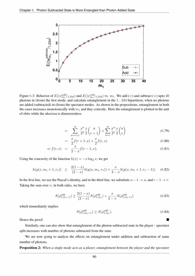
Chapter 6. Photon Subtracted State is More Entangled than Photon Added State

0

0.5

1

1.5

2

2.5

3

0 5 10 15 20 25 30 35 40

E(|

ψm

1

ad

d/s

ub⟩ 1

:234)

m1

Sub

Add

Figure 6.3: Behavior of E(| addm1i1:234) and E(| sub

m1i1:234) vs. m1. We add (⇥) and subtract (+) upto 40

photons in (from) the first mode, and calculate entanglement in the 1 : 234 bipartition, when no photonsare added (subtracted) in (from) the spectator modes. As shown in the propositions, entanglement in boththe cases increases monotonically with m1 and they coincide. Here the entanglement is plotted in the unitof ebits while the abscissa is dimensionless.

=1X

n=r+1

xn

2nx

2

✓n

r + 1

◆+1X

n=r

xn

2nx

2

✓n

r

◆(6.79)

=x

2f(r + 1, x) +

x

2f(r, x) (6.80)

) f(r, x) =x

2� xf(r � 1, x). (6.81)

Using the concavity of the function h(x) = �x log2 x, we get

h(g(x,m1 + 1, r1)) �2(1� x)

(2� x)h(g(x,m1, r1)) +

x

2� xh(g(x,m1 + 1, r1 � 1)). (6.82)

In the first line, we use the Pascal’s identity, and in the third line, we substitute n� 1! n, and r� 1! r.Taking the sum over r1 in both sides, we have

S(⇢add1,m1+1) �2(1� x)

(2� x)S(⇢add1,m1

) +x

2� xS(⇢add1,m1+1) (6.83)

which immediately impliesS(⇢add1,m1+1) � S(⇢add1,m1

). (6.84)

Hence the proof. ⌅Similarly, one can also show that entanglement of the photon-subtracted state in the player : spectator

split increases with number of photons subtracted from the state.We are now going to analyze the e�ects on entanglement under addition and subtraction of same

number of photons.Proposition 2: When a single mode acts as a player, entanglement between the player and the spectator

90

6.4. Comparison of entanglement enhancement between photon addition and subtraction

modes of the photon-added state coincide with that of the photon-subtracted state.Proof: To prove that the increase of entanglement in the multimode state is same for addition andsubtraction, we consider the single mode reduced density matrix. The single site reduced density matrixof photon-subtracted state, after inserting N

sub1 , is given by

⇢sub1,m1

= (1� x)m1+11X

r1=0

✓m1 + r1

m1

◆ 1X

n=r1

xn

2n

✓n+m1

r1 +m1

◆

| {z }fsub(r1,m1,x)

|r1ihr1|. (6.85)

Now fsub(r1,m1, x) can be evaluated by substituting n� r1 ! n, r1 +m1 ! m and x2 ! v,

fsub(r1,m1, x) =xr1

2r1

1X

n=0

vn

✓n+m

m

◆=

xr1

2r1

1X

n=0

1

m!

dm

dvmvn+m

=1

m!

xr1

2r1dm

dvm

vm

1� v=

xr1

2r1(1� v)�m�1

=xr12m1+1

(2� x)m1+r1+1. (6.86)

On the other hand, the reduced density matrix after adding same number of photons reads as

⇢add1,m1

=1X

r1=0

2m1(1� x)m1+1

(2� x)m1

2

2� x

⇣x

2� x

⌘r1✓m1 + r1

m1

◆|r1 +m1ihr1 +m1|. (6.87)

The above form has been obtained by substituting Eq. (6.77) of f(r, x) in Eq. (6.70), which is

f(r, x) =x

2� xf(r � 1, x) =

xr

(2� x)rf(0, x),

=xr

(2� x)r

1X

n=0

xn

2n=

xr

(2� x)r2

(2� x)(6.88)

Comparing Eqs. (6.85) and (6.87), we have S(⇢add1,m1) = S(⇢sub1,m1

). ⌅To visualize the above Propositions, we plot S(⇢add/sub1,m1

), with respect to m1 by fixing the squeezingparameter r = 0.4 in Fig. 6.3. It clearly shows that the curve for photon addition merges with the curveof photon subtraction. Moreover, it shows that entanglement in that bipartition monotonically increaseswith the addition or subtraction of photons as shown in Proposition 1. Note here that although the resultspresented here are when the photons are added at the mode 1 and the bipartition is considered as player: spectator mode, the Propositions remain unaltered if another mode also acts as a player by keeping thesimilar bipartition.

E�ects on entanglement due to change of player modes

We now consider the entanglement in the same bipartition as in the previous case, i.e., 1 : 234. However,the second or third mode now act as player and no photons are added in the rest of the modes. In theprevious case, one block contained only the player mode while the other one contains all the spectatormodes. In this case, one part of the partition contains one spectator mode while the other one consistsof both the player and the rest of the spectator modes. In the previous case, we have already shown that

91

Chapter 6. Photon Subtracted State is More Entangled than Photon Added State

0

1

2

3

4

0 10 20 30 40

E(|

ψm

2

add/s

ub⟩ 1

:23

4)

m2

(a)

Sub Add

0

1

2

3

0 10 20 30 40

E(|

ψm

3

add/s

ub⟩ 1

:23

4)

m3

(b)

Sub Add

Figure 6.4: (a) Trends ofE(| addm2i1:234) andE(| sub

m2i1:234)with the number of photon-added (subtracted)

in (from) the second mode. (b) Similar study has been carried out when the third mode acts as a player.Both the cases reveal that subtraction is better than addition. Ordinates are plotted in the unit of ebitswhile the abscissas are dimensionless.

the e�ects on entanglement due to addition and subtraction of photons are similar. We will now showwhether such observation remains invariant even in this scenario.

Let us now take the four-mode squeezed vacuum state as input, and add (subtract) m2 photons in(from) the second mode. As depicted in Fig. 6.4(a), we find that unlike the previous case, the photon-subtracted state possesses more entanglement in the 1 : 234 bipartition than that of the photon-addedstate. The ordering remains unchanged if one takes the third mode as player and consider entanglementin the 1 : 234 split (see Fig. 6.4(b)). Moreover, we observe that the amount of entanglement decreases inthis scenario, compared to the case when the second mode acts as a player. Note here that if one takes thetwo-mode squeezed vacuum state as input, it was observed that the bipartite entanglement content of thephoton-subtracted state is always lower than that of the photon-added state.

Bipartition with both player and spectator modes

We still restrict ourselves to the case of a single player. But we now move to the situations in whichentanglement of a four-mode state is studied by considering a bipartition in which both sides of the splitcontain two modes, namely 12 : 34 and 13 : 24. The other split between modes, i.e., 14 : 23, reflects asimilar behavior, due to the symmetry of the four-mode state. In these two scenarios, photons are addedor subtracted in the first mode, as shown in Fig. 6.5, and no photons are added or subtracted, in the otherspectator modes.

To study entanglement of | addm1i (| sub

m1i) in the 12 : 34 or 13 : 24 bipartition, we require the two party

reduced density matrices, ⇢add12,m1, ⇢add13,m1

, ⇢sub12,m1, and ⇢sub13,m1

. We have

⇢add12,m1

=1

Nadd12

1X

n,n0=0

x(n+n0)/2

2n+n0

min{n,n0}X

r1,r2=0

s✓n

r1

◆✓n

r2

◆s✓n0

r1

◆✓n0

r2

◆s(n+m1 � r1)!

(n� r1)!

⇥

s(n0 +m1 � r1)!

(n0 � r1)!|n+m1 � r1i1|n� r2i2hn

0 +m1 � r1|1hn0� r2|2, (6.89)

92

6.4. Comparison of entanglement enhancement between photon addition and subtraction

Figure 6.5: Schematic diagram of two di�erent blocks, when a single mode, specifically the first mode,acts as a player.

and

⇢sub12,m1

=1

Nsub12

1X

n,n0=m1

x(n+n0)/2

2n+n0

min{n,n0}�m1X

r1=0

min{n,n0}X

r2=0

s✓n

r1

◆✓n

r2

◆s✓n0

r1

◆✓n0

r2

◆s(n� r1)!

(n�m1 � r1)!

⇥

s(n0 � r1)!

(n0 �m1 � r1)!|n�m1 � r1i1|n� r2i2hn

0�m1 � r1|1hn

0� r2|2. (6.90)

Note that in the previous cases, where one partition contains only a single mode, we required single-sitedensity matrices to calculate the entanglement, and they are always diagonal in the number basis. Thesame is not the case for two-site density matrices. Similarly, one can find out the reduced density matricesof ⇢add13,m1

and ⇢sub13,m1. In both the scenarios, we observe that entanglement increases against the number

of photons added, m1 and same is true for subtraction of photons (see Fig. 6.6). Moreover, as observedin the previous case with the smallest partition consisting of the spectator mode, photon-subtracted statecontains higher entanglement in the 12 : 34 as well as 13 : 24 partitions than that of the correspondingphoton-added state. See Figs. 6.6(a) and 6.6(b).

We briefly mention here the method used to calculate S(⇢add12,m1), and the other local entropies. The

von Neumann entropy of ⇢add12,m1can be obtained if one can diagonalize the infinite dimensional matrix,

given in Eq. (6.89). To calculate it, for fixed m1, we have to truncate the summation upto a large valueof n and n

0, say N for both, and calculate its trace, i.e., trN (⇢add12,m1), as well as von Neumann entropy,

SN (⇢add12,m1

). We then choose, 2N as maximum of n and n0 and obtain the quantities. When the di�erence

between SN (⇢add12,m1

) and S2N (⇢add12,m1

) is of the order of 10�6, we take SN (⇢add12,m1) as the actual entropy.

In Fig 6.7, for a fixed value of m1, we plot SN (⇢add12 ) and trN (⇢add12 ) with the variation of N . With theincrease of m1, we observe that we require higher values of N . However, the figure shows both thequantities converge when N � 10, irrespective of the value of m1. When we compute entropy or LN, we

93

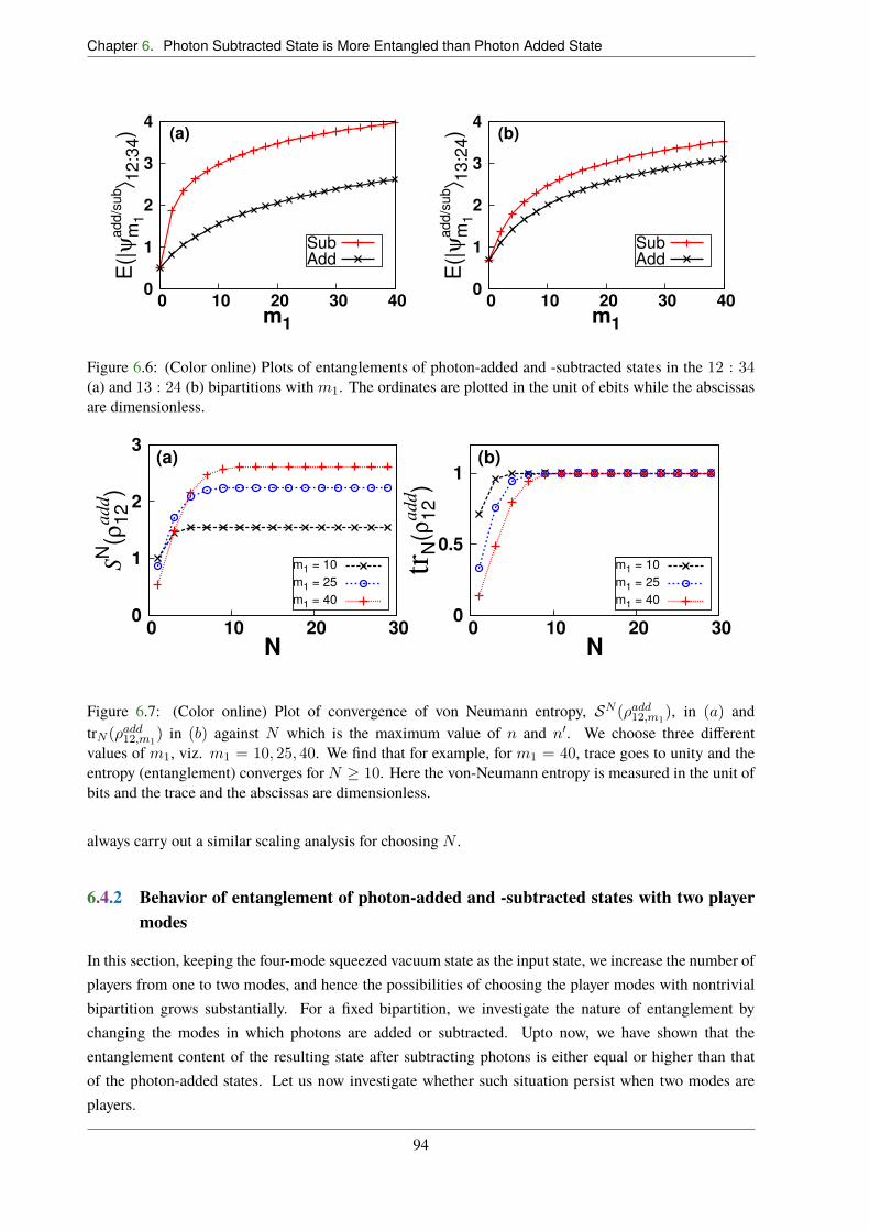
Chapter 6. Photon Subtracted State is More Entangled than Photon Added State

0

1

2

3

4

0 10 20 30 40

E(|

ψm

1

add/s

ub⟩ 1

2:3

4)

m1

(a)

Sub Add

0

1

2

3

4

0 10 20 30 40

E(|

ψm

1

add/s

ub⟩ 1

3:2

4)

m1

(b)

Sub Add

Figure 6.6: (Color online) Plots of entanglements of photon-added and -subtracted states in the 12 : 34(a) and 13 : 24 (b) bipartitions with m1. The ordinates are plotted in the unit of ebits while the abscissasare dimensionless.

0

1

2

3

0 10 20 30

SN

(ρ12

add)

N

(a)

m1 = 10

m1 = 25

m1 = 40

0

0.5

1

0 10 20 30

trN

(ρ12

add)

N

(b)

m1 = 10

m1 = 25

m1 = 40

Figure 6.7: (Color online) Plot of convergence of von Neumann entropy, SN (⇢add12,m1

), in (a) andtrN (⇢add12,m1

) in (b) against N which is the maximum value of n and n0. We choose three di�erent

values of m1, viz. m1 = 10, 25, 40. We find that for example, for m1 = 40, trace goes to unity and theentropy (entanglement) converges for N � 10. Here the von-Neumann entropy is measured in the unit ofbits and the trace and the abscissas are dimensionless.

always carry out a similar scaling analysis for choosing N .

6.4.2 Behavior of entanglement of photon-added and -subtracted states with two playermodes

In this section, keeping the four-mode squeezed vacuum state as the input state, we increase the number ofplayers from one to two modes, and hence the possibilities of choosing the player modes with nontrivialbipartition grows substantially. For a fixed bipartition, we investigate the nature of entanglement bychanging the modes in which photons are added or subtracted. Upto now, we have shown that theentanglement content of the resulting state after subtracting photons is either equal or higher than thatof the photon-added states. Let us now investigate whether such situation persist when two modes areplayers.

94

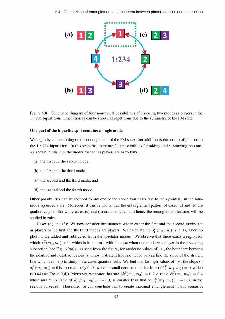
6.4. Comparison of entanglement enhancement between photon addition and subtraction

Figure 6.8: Schematic diagram of four non-trivial possibilities of choosing two modes as players in the1 : 234 bipartition. Other choices can be shown as repetitions due to the symmetry of the FM state.

One part of the bipartite split contains a single mode

We begin by concentrating on the entanglement of the FM state after addition (subtraction) of photons inthe 1 : 234 bipartition. In this scenario, there are four possibilities for adding and subtracting photons.As shown in Fig. 6.8, the modes that act as players are as follows:

(a) the first and the second mode,

(b) the first and the third mode,

(c) the second and the third mode, and

(d) the second and the fourth mode.

Other possibilities can be reduced to any one of the above four cases due to the symmetry in the four-mode squeezed state. Moreover, it can be shown that the entanglement pattern of cases (a) and (b) arequalitatively similar while cases (c) and (d) are analogous and hence the entanglement features will bestudied in pairs.

Cases (a) and (b): We now consider the situation where either the first and the second modes actas players or the first and the third modes are players. We calculate the �E1 (m1,mi) (i 6= 1), when nophotons are added and subtracted from the spectator modes. We observe that there exists a region forwhich �E1 (m1,mi) > 0, which is in contrast with the case when one mode was player in the precedingsubsection (see Fig. 6.9(a)). As seen from the figure, for moderate values of m1, the boundary betweenthe positive and negative regions is almost a straight line and hence we can find the slope of the straightline which can help to study these cases quantitatively. We find that for high values of m1, the slope of�E1 (m1,m3) = 0 is approximately 0.28, which is small compared to the slope of �E1 (m1,m2) = 0, which

is 0.64 (see Fig. 6.9(d)). Moreover, we notice that max [�E1 (m1,m3)] = 0.2 < max [�E1 (m1,m2)] = 0.4

while minimum value of �E1 (m1,m3)(= �2.0) is smaller than that of �E1 (m1,m2)(= �1.6), in theregions surveyed. Therefore, we can conclude that to create maximal entanglement in this scenario,

95

Chapter 6. Photon Subtracted State is More Entangled than Photon Added State

Figure 6.9: Top panel: Behavior of �E1 (m1,m3) against m1 (horizontal axes) and m3 (vertical axes)when the spectator modes are active, figure(a) both m2 = m4 = 0, figure (b) m2 = 5, m4 = 0 andin figure (c) m2 = m4 = 5. We see that by using fixed number of photons to the spectators modes,entanglement of photon added state can be enhanced much faster than the photon subtracted ones. Bottompanel: Similar behavior of �E1 (m1,m2) against m1 (horizontal axes) and m2 (vertical axes), when nophotons are added in the spectator mode (figure (d)), only one spectator mode is active, m3 = 5, m4 = 0in figure (e) and m3 = 0, m4 = 5 in figure (f). We find that the region where photon addition is betterthan the subtraction remains almost constant. All the axes are dimensionless, while entanglements areplotted in the unit of ebits.

photon addition is advantageous when one adds photons in the first and the second modes compared tothe case of m1 and m3 being players (with m1 � mi, i = 2, 3).

In both the cases, spectator modes play an important role in the behavior of entanglement in the1 : 234 bipartition. As depicted in Fig. 6.9 (b), entanglement in the photon-added state can be increasedby adding photons in the spectator modes. For example, when m2(4) = 5, �E1 (m1,m3) against m1 andm3 is depicted in Fig. 6.9(b) and for both m2 = m4 = 5 in Fig. 6.9(c) . Quantitative comparison can bemade between Figs. 6.9 (c) and 6.9 (d). In particular, for m1 � m3, the region with �E1 (m1,m3) > 0

when no photons are added (subtracted) in the spectator modes can be calculated. In this limit, we assumethat the boundary is a straight line and hence the area is the area of a quadrilateral. Let us call the areaas �0. In this case, we calculate the area of the quadrilateral when m1 � 25 and m1 40, and we find�0 ⇡ 160. After adding (subtracting) 5 photons in the second or fourth modes, we find that the area,�5, of the corresponding quadrilateral increases and �5 ⇡ 253. Moreover the area increases much more,as shown in Fig. 6.9 (c), when both the spectator modes are active, and in such a situation �5,5 ⇡ 425.But the scenario is something di�erent in the case of �E1 (m1,m2) > 0, the area where photon additionproduce much more entanglement than photon subtraction, is more or less invariant when the spectatormodes are active, as shown in Figs. 6.9 (d), 6.9 (e) and 6.9 (f).

96

6.4. Comparison of entanglement enhancement between photon addition and subtraction

(i) (ii)

Figure 6.10: Distinct scenarios of the bipartition containing two modes and two player modes in the13 : 24 split (figure (i)) and 12 : 34 (figure (ii)). For the 13 : 24 bipartition there are two possibilities –(a) first and second as players, (b) first and third as players. In the 12 : 34 split one can chose – (a) firstand second as players, (b) first and third as players, and (c) first and forth as player.

Behavior of entanglement in the 1 : 234 split for cases (c) and (d) are almost identical with theprevious cases. The only di�erence is that entanglement of the subtracted state is always better than thatof the added state when spectator modes are inactive. The picture changes, i.e. entanglement of thephoton-added states starts increasing faster than the photon-subtracted states, like in the preceding cases,when fixed numbers of photons are added (subtracted) in the spectator mode(s).

Bipartition containing equal number of modes

We will now consider the case where, we still keep two modes as players but we now divide four-modesinto two blocks consisting of two modes instead of one mode in the preceding discussion. In this case, thetwo nontrivial bipartitions are 12 : 34 and 13 : 24. Let us first concentrate on the bipartition 13 : 24. Inthis case, the symmetry of the FMSV state after addition or subtraction of arbitrary number of photons inall the modes, given in Eqs. (6.60) and (6.61), ensures that there are only two nontrivial situations in thecase of two player modes (see Fig. 6.10 (i)) . They are – (a) when the players are the first and the secondmodes, and (b) when first and third modes act as players. Cases (a) and (b) show similar entanglementbehavior like previous cases, when one part of the bipartition contains a single mode, but the region wherethe photon addition is much more better than the subtraction changes it form in the plane of the playermodes. Here we will briefly analyze this situations.

The reduced density matrix of the first and the third mode, for the photon-added state, is given by

⇢add13,{mi} = tr24(| add

{mi}ih add{mi}|)

=1X

n=0

nX

r1=0

an,r1,q|n+m1 � r1i1|m3 + r1i3hn+m1 � q|1hm3 + q|3, (6.91)

97

Chapter 6. Photon Subtracted State is More Entangled than Photon Added State

Figure 6.11: Role of spectator modes in �E13 in the plane of m1,m2 and m1,m3 when the player modesare active. In (a), m3 = 10 and m4 = 0, while in (b), m3 = m4 = 5. We see that spectator modeshelp to enhance entanglement in the photon-added state. In (c) no spectator mode is active, and a positiveregion emerges around the line m1 = m3 > 14, which can be enhanced more when one spectator modeis active, as shown in (d) where m2 = 4. All the axes are dimensionless, while entanglements are plottedin the unit of ebits.

where we write

an,r1,q =1

Nadd13

xn

2n

nX

r2=0

⇣✓n

r1

◆✓n

q

◆⌘1/2✓n

r2

◆⇣(n+m1 � r1)!

(n� r1)!

(n+m1 � q)!

(n� q)!

(m3 + r1)!

r1!

(m3 + q)!

(q)!

⌘1/2

(n+m2 � r2)!

(n� r2)!

(m4 + r2)!

r2!. (6.92)

Similarly, one can also find the two party reduced density matrix, ⇢sub13,{mi}, for photon subtraction bytracing out the second and fourth modes in Eq. (6.61).

Case (a): If the first and second modes act as players, we find that subtraction is always better thanaddition for arbitrary values of m1 and m2. This case is similar to the case with a single mode being playerand cases with second and third modes or second and fourth modes being players. To show once morethat spectators play a fundamental role in interchanging the entanglement property for photon additionand subtraction, we elaborate the analysis in two scenarios – (1) when a fixed number of photons areadded (subtracted) in a single spectator mode, a positive region emerges, which indicates that the quantumcorrelation in the 13 : 24 bipartition is greater for photon addition than that for subtraction, as alreadyseen before. An interesting point to note here is that a positive region appears for small values of m2 andalmost for all values of m1. This is probably due to the fact that we add photons in the third mode which

98

6.5. Comparison of logarithmic negativity between two-mode and four-mode states

belongs to the same block as the first mode. (2) When both the spectator modes are active, the positiveregion can be seen in both the axis due to symmetry present in the FM state, as depicted in Fig. 6.11(b).Case (b): When the first and third mode are chosen as player a small region emerges, where photonaddition is better than the photon subtraction, in the plane of m1 and m3, in the vicinity of m1 = m2.The region exists for m1(3) > 14, as shown in Fig. 6.11(c). This region increases as one make anyone of the spectator modes active, and it increases much rapidly with the increase of number of photonadded(subtracted) from the spectator mode, keep subtraction better than addition in the vicinity of m1 ⇡ 0

and m3 ⇡ 0, near about the axes. Fig 6.11(d) shows the emergence of this positive area for m2 = 4.Finally, we concentrate on a nontrivial partition, the 12 : 34 cut (see Fig. 6.10(ii)). From the

perspective of entanglement, this partition is unique. In this scenario, there are three ways to choosethe players. We find that with and without participation of spectator modes, entanglement of photonsubtraction always higher or equal to that of the photon addition which makes this situation exclusive fromothers.

6.5 Comparison of logarithmic negativity between two-mode and four-mode states

Upto now, we have considered an FMSV state as input and have compared the behavior of entanglementbetween photon-added and -subtracted states as well as entanglement of an output state in di�erentbipartitions having di�erent player and spectator modes. In this section, our aim is to make comparisonbetween the output state obtained from the TMSV state after adding or subtracting photons and the twomode state obtained from the FMSV state. To perform such comparison, we discard two modes from thefour-mode state and calculate the LN of the two mode reduced state, which we then compare with the LNof the photon-added (subtracted) state that is obtained from the TMSV state as the input [51–54]. In caseof the TM state, the output state, after adding (subtracting) photons, still remains pure and hence LN canbe calculated analytically [198]. However, for the FM case, the output state is mixed which is obtainedby discarding two modes and we adopt the same mechanism as we have done to calculate von Neumannentropy of reduced density matrices, described in Sec. 6.4.1. In particular, we evaluate LN as well astrace for large n = N , and then by increasing N , we check whether trace goes to unity upto six decimalpoints. We truncate the system when trace has already converged to unity, upto six decimal points.

In the TMSV case, photons can be added to either of the modes or to both the modes. On the otherhand, there are several scenarios for the four-mode states. If there is a single player, either one of the modeof the output state can act as player or none of the modes of the output state is the player. In case of twoplayers, (i) two players can be the two modes of the output state, (ii) one mode of the output state can bea player, or (iii) the discarded modes can be the player modes.

Before considering the FMSV state, let us first consider the TMSV state as input. Note that the natureof LN qualitatively matches with the von Neumann entropy of the reduced density matrix. As shownin [51–54], when single mode acts as player, the LN for photon addition coincide with the subtraction,which is also the case for the von Neumann entropy. If both the modes act as players, photon addition isalways beneficial for entanglement than the photon subtraction [51–54].

In case of a single player or two players in the FM state, if the output state contains the player mode(s),then the reduced two-mode state obtained from the photon-added state has higher LN than that of the

99

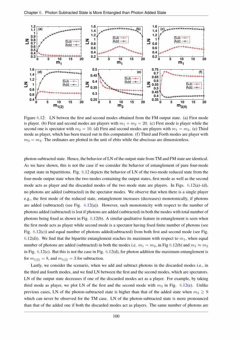
Chapter 6. Photon Subtracted State is More Entangled than Photon Added State

0.3 0.4 0.5 0.6 0.7 0.8 0.9

1 1.1 1.2

0 5 10 15 20

LN

m1

(a)

Sub Add

0.2

0.4

0.6

0.8

1

1.2

1.4

1.6

0 5 10 15 20

LN

m1

(b)

Sub Add

0.2

0.4

0.6

0.8

1

1.2

1.4

1.6

0 5 10 15 20

LN

m1

(c)

Sub Add

0.4

0.6

0.8

1

1.2

1.4

1.6

0 5 10 15 20

LN

m1(2)

(d)

Sub Add

0.25

0.3

0.35

0.4

0.45

0.5

0 5 10 15 20

LN

m3

(e)

Sub Add

0.35 0.4

0.45 0.5

0.55 0.6

0.65 0.7

0.75

0 5 10 15 20

LN

m3(4)

(f)

Sub Add

Figure 6.12: LN betwen the first and second modes obtained from the FM output state. (a) First modeis player. (b) First and second modes are players with m1 +m2 = 20. (c) First mode is player while thesecond one is spectator with m2 = 10. (d) First and second modes are players with m1 = m2. (e) Thirdmode as player, which has been traced out in this computation. (f) Third and Forth modes are player withm3 = m4. The ordinates are plotted in the unit of ebits while the abscissas are dimensionless.

photon-subtracted state. Hence, the behavior of LN of the output state from TM and FM state are identical.As we have shown, this is not the case if we consider the behavior of entanglement of pure four-modeoutput state in bipartitions. Fig. 6.12 depicts the behavior of LN of the two-mode reduced state from thefour-mode output state when the two modes containing the output states, first mode as well as the secondmode acts as player and the discarded modes of the two mode state are players. In Figs. 6.12(a)–(d),no photons are added (subtracted) in the spectator modes. We observe that when there is a single playere.g., the first mode of the reduced state, entanglement increases (decreases) monotonically, if photonsare added (subtracted) (see Fig. 6.12(a)). However, such monotonicity with respect to the number ofphotons added (subtracted) is lost if photons are added (subtracted) in both the modes with total number ofphotons being fixed as shown in Fig. 6.12(b). A similar qualitative feature in entanglement is seen whenthe first mode acts as player while second mode is a spectator having fixed finite number of photons (seeFig. 6.12(c)) and equal number of photons added(subtracted) from both first and second mode (see Fig.6.12(d)). We find that the bipartite entanglement reaches its maximum with respect to m1, when equalnumber of photons are added (subtracted) in both the modes i.e. m1 = m2, in Fig 6.12(b) and m1 ⇡ m2

in Fig. 6.12(c). But this is not the case in Fig. 6.12(d), for photon addition the maximum entanglement isfor m1(2) = 8, and m1(2) = 3 for subtraction.

Lastly, we consider the scenario, when we add and subtract photons in the discarded modes i.e., inthe third and fourth modes, and we find LN between the first and the second modes, which are spectators.LN of the output state decreases if one of the discarded modes act as a player. For example, by takingthird mode as player, we plot LN of the first and the second mode with m3 in Fig. 6.12(e). Unlikeprevious cases, LN of the photon-subtracted state is higher than that of the added state when m3 � 9

which can never be observed for the TM case. LN of the photon-subtracted state is more pronouncedthan that of the added one if both the discarded modes act as players. The same number of photons are

100

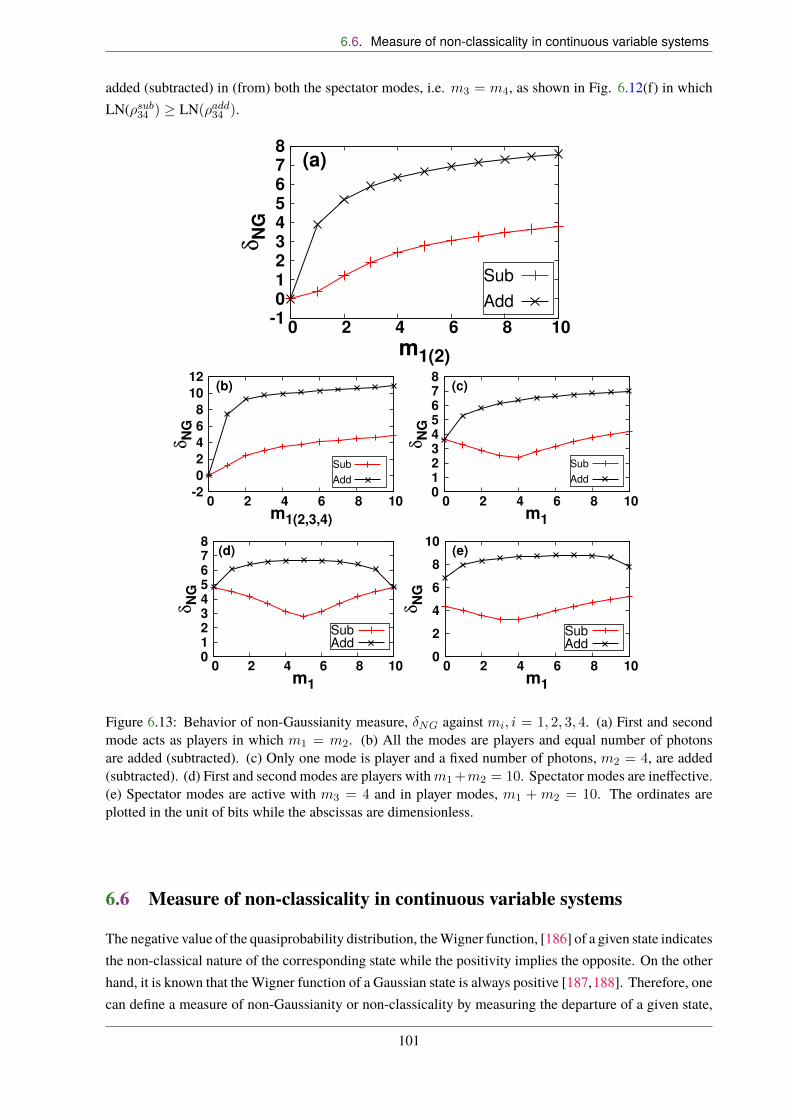
6.6. Measure of non-classicality in continuous variable systems

added (subtracted) in (from) both the spectator modes, i.e. m3 = m4, as shown in Fig. 6.12(f) in whichLN(⇢sub34 ) � LN(⇢add34 ).

-1 0 1 2 3 4 5 6 7 8

0 2 4 6 8 10

δNG

m1(2)

(a)

Sub

Add

-2

0

2

4

6

8

10

12

0 2 4 6 8 10

δNG

m1(2,3,4)

(b)

Sub

Add

0 1 2 3 4 5 6 7 8

0 2 4 6 8 10

δNG

m1

(c)

Sub

Add

0 1 2 3 4 5 6 7 8

0 2 4 6 8 10

δNG

m1

(d)

Sub Add

0

2

4

6

8

10

0 2 4 6 8 10

δNG

m1

(e)

Sub Add

Figure 6.13: Behavior of non-Gaussianity measure, �NG against mi, i = 1, 2, 3, 4. (a) First and secondmode acts as players in which m1 = m2. (b) All the modes are players and equal number of photonsare added (subtracted). (c) Only one mode is player and a fixed number of photons, m2 = 4, are added(subtracted). (d) First and second modes are players with m1+m2 = 10. Spectator modes are ine�ective.(e) Spectator modes are active with m3 = 4 and in player modes, m1 + m2 = 10. The ordinates areplotted in the unit of bits while the abscissas are dimensionless.

6.6 Measure of non-classicality in continuous variable systems

The negative value of the quasiprobability distribution, the Wigner function, [186] of a given state indicatesthe non-classical nature of the corresponding state while the positivity implies the opposite. On the otherhand, it is known that the Wigner function of a Gaussian state is always positive [187,188]. Therefore, onecan define a measure of non-Gaussianity or non-classicality by measuring the departure of a given state,

101

Chapter 6. Photon Subtracted State is More Entangled than Photon Added State

⇢, in a CV system from a Gaussian state. In terms of relative entropy distance, it is given by [206–208]

�NG(%) = S(%||%G) = S(%G)� S(%), (6.93)

where S(⌘||�) = �tr(⌘ log2 �)�S(⌘), and ⇢G is a Gaussian state which has same covariance matrix andfirst moment as ⇢. Here, S(�) = �tr(� log2 �) is the von Neumann entropy of �.

For an N -mode continuous variable system ⇢, with quadrature operators {qj , pj}, j = 1, . . . , N , thecovariance matrix � is given by

�jk =1

2h⇠j ⇠k + ⇠k⇠ji � h⇠jih⇠ki, (6.94)

where the expectation is computed with respect to the state ⇢ and

⇠ = (q1 p1 q2 p2 · · · qN pN )T . (6.95)

The von Neumann entropy, S(%G), of any Gaussian state can be calculated by using its covariance matrix,�. For an N mode Gaussian state, %G, the von Neumann entropy is defined [36] as

S(%G) =NX

k=1

g(⌫k), (6.96)

where ⌫k is the Williamson normal form [209] of the covariance matrix of the N -mode Gaussian state%G, and the function g(x) is given by

g(x) = �x+ 1

2log2

⇣x+ 1

2

⌘�

x� 1

2log2

⇣x� 1

2

⌘. (6.97)

As we have mentioned in the earlier section that the photon addition and subtraction is one of the ways tocreate a non-Gaussian state. Here, we quantify the departure of the photon-added (-subtracted) FMSV statefrom Gaussianity, as a function of added (subtracted) photons from the player modes. Since the photon-added (-subtracted) FM state is in a pure state, the second term of �NG(⇢), given in Eq. (6.93) vanishes. Tocalculate �NG(⇢), we have to find the covariance matrix of ⇢G, which is same as ⇢add/sub{mi} = | ih |

add/sub{mi} .

It is given by

�% =

0

BBBBBBBBB@

hq21iI hq1q2i�z hq1q3iI hq1q4i�z

hq1q2i�z hq22iI hq2q3i�z hq2q4iI

hq1q3iI hq2q3i�z hq23iI hq3q4i�z

hq1q4i�z hq2q4iI hq3q4i�z hq24iI

1

CCCCCCCCCA

, (6.98)

where, qi = ai+ a†i , and the expectations are taken over the photon-added and -subtracted FM state, given

in Eqs. (6.60) and (6.61) and

hq21i

add = 1 + 2m1 + 2X

n,r1,r2

(p{mi}n,r1,r2)

2(n� r1), hq22i

add = 1 + 2m2 + 2X

n,r1,r2

(p{mi}n,r1,r2)

2(n� r2),

hq23i

add = 1 + 2m3 + 2X

n,r1,r2

(p{mi}n,r1,r2)

2r1, hq

24i

add = 1 + 2m4 + 2X

n,r1,r2

(p{mi}n,r1,r2)

2r2,

102

6.6. Measure of non-classicality in continuous variable systems

hq1q2iadd = 2

X

n,r1,r2

p{mi}n,r1,r2p

{mi}n+1,r1,r2 ⇥

p(n+m1 � r1 + 1)(n+m2 � r2 + 1),

hq1q3iadd = 2

X

n,r2

n�1X

r1=0

p{mi}n,r1,r2p

{mi}n,r1+1,r2

p(n+m1 � r1)(m3 + r1 + 1),

hq1q4iadd = 2

X

n,r1,r2

p{mi}n,r1,r2p

{mi}n+1,r1,r2+1 ⇥

p(n+m1 � r1 + 1)(m4 + r2 + 1),

hq2q3iadd = 2

X

n,r1,r2

p{mi}n,r1,r2p

{mi}n+1,r1+1,r2 ⇥

p(n+m2 � r2 + 1)(m3 + r1 + 1),

hq2q4iadd = 2

X

n,r1

n�1X

r2=0

p{mi}n,r1,r2p

{mi}n,r1,r2+1 ⇥

p(n+m2 � r2)(m4 + r2 + 1),

hq3q4iadd = 2

X

n,r1,r2

p{mi}n,r1,r2p

{mi}n+1,r1+1,r2+1 ⇥

p(m3 + r1 + 1)(m4 + r2 + 1),

whereP

n,r1,r2in the photon-added states, is the short form of

Pn=0

Pnr1=

Pnr2=0. Further, for the

photon-subtracted states,

hq21i

sub = 1� 2m1 + 2X

n,r1,r2

(q{mi}n,r1,r2)

2(n� r1), hq22i

sub = 1� 2m2 + 2X

n,r1,r2

(q{mi}n,r1,r2)

2(n� r2),

hq23i

sub = 1� 2m3 + 2X

n,r1,r2

(q{mi}n,r1,r2)

2r1, hq

24i

sub = 1� 2m4 + 2X

n,r1,r2

(q{mi}n,r1,r2)

2r2,

hq1q2isub = 2

X

n,r1,r2

q{mi}n,r1,r2q

{mi}n+1,r1,r2 ⇥

p(n�m1 � r1 + 1)(n�m2 � r2 + 1),

hq1q2isub = 2

X

n,r1,r2

q{mi}n,r1,r2q

{mi}n+1,r1,r2 ⇥

p(n�m1 � r1 + 1)(n�m2 � r2 + 1),

hq1q3isub = 2

X

n,r2

n�m1�1X

r1=m3

q{mi}n,r1,r2p

{mi}n,r1+1,r2 ⇥

p(n�m1 � r1)(r1 �m3 + 1),

hq1q4isub = 2

X

n,r1,r2

q{mi}n,r1,r2q

{mi}n+1,r1,r2+1 ⇥

p(n�m1 � r1 + 1)(r2 �m4 + 1),

hq2q3isub = 2

X

n,r1,r2

q{mi}n,r1,r2q

{mi}n+1,r1+1,r2 ⇥

p(n�m2 � r2 + 1)(r1 �m3 + 1),

hq2q4isub = 2

X

n,r1

n�m2�1X

r2=m4

q{mi}n,r1,r2q

{mi}n,r1,r2+1 ⇥

p(n�m2 � r2)(r2 �m4 + 1),

hq3q4isub = 2

X

n,r1,r2

q{mi}n,r1,r2q

{mi}n+1,r1+1,r2+1 ⇥

p(r1 �m3 + 1)(r2 �m4 + 1),

whereP

n,r1,r2, is the short form of

Pn=M

Pn�m1r1=m3

Pn�m2r2=m4

, and M = max{m1 + m3,m2 + m4}.The p{mi}

n,r1,r2 and q{mi}n,r1,r2 are given in Eqs. (6.60) and (6.61) respectively.

The Williamson normal form of Eq. (6.98) can be evaluated by using the prescription given in [210].We numerically calculate the Williamson normal form of the matrix in Eq. (6.98) for both photon additionand subtraction and calculate the non-Gaussianity, which in this case reduces to S(⇢add/subG,{mi} ).

In all the cases, photon addition leads to a rapid departure of Gaussianity than that of the photonsubtraction. We also notice that if among four modes, photons are added only in two modes, then behaviorof �NG obtained in the FM state and the TM state are qualitatively similar. It is clear from the behavior

103

Chapter 6. Photon Subtracted State is More Entangled than Photon Added State

of the non-Gaussianity measure that photon-subtracted state become slowly non-Gaussian as comparedto the photon-added state and the behavior remains unchanged irrespective of the choices of the playerand the spectator modes (see Fig. 6.13). The rich picture of the role of di�erent modes, captured byentanglement, is not seen by the non-Gaussianity measure and hence indicates that there is possibly nodirect connection between non-Gaussianity and entanglement content of the output state obtained afterphoton addition (subtraction) [51–54].

6.7 In Closing

In this chapter, we discuss the N -mode squeezed vacuum state, and find its form in terms of the Focknumber basis forN = 2, TMSV state and forN = 4, FMSV state. We have also discussed the procedure toprepare the FMSV state in the laboratory by using linear optical devices. Photon addition and subtractionconstitute useful methods to prepare non-Gaussian states. It has already been established that non-Gaussian states are useful in various quantum mechanical tasks ranging from entanglement distillation toquantum error correction. We have investigated the entanglement properties of the non-Gaussian statesgenerated by adding or subtracting photons in Gaussian states. In case of two mode states, entanglementof photon-added states is known to be equal or higher than that of the photon-subtracted ones.

We have shown that this is not the case when one increases the number of modes. We found thatfor four-mode states, the trend of entanglement distribution in di�erent bipartitions of the photon-added(-subtracted) states is much richer than that in the two-mode states. Specifically, we showed that thereexists a scenario, in which multimode entanglement content of the photon-subtracted state is always higherthan that of the corresponding photon-added one. The results remained unchanged even if one discardedtwo modes from the four-mode output state. Moreover, we showed that the picture that emerges fromentanglement of the output state does not match with the behavior in the same states of distance-basednon-Gaussianity measure. Upto now, it was known that among addition and subtraction, addition is morebeneficial. But our work shows that photon subtraction can also be advantageous if we consider a state ofa higher number of modes.

The main motivation to study such four-mode entangled state is to use this kind of states in commu-nication protocols like, for example, the distributed dense coding with two senders and two receivers. Webelieve that by taking the four-mode squeezed vacuum state as the resource state quantum communicationnetworks like the ones described in preceding chapters can be built by using continuous variable systemsin near future, and our investigation on entanglement patterns of non-Gaussian multimode states is ansmall step towards that.

The results of this Chapter are based on the following paper:

1. Subtraction better than addition: Entanglement in multimode squeezed vacuum post-interface withphotons, Tamoghna Das, R. Prabhu, Aditi Sen De, Ujjwal Sen, Phys. Rev. A 93, 052313 (2016).

104

Chapter 7Summary and Future Directions

In last few decades, it has been established that bipartite as well as multipartite quantum correlations (QC),in particular, entanglement plays a crucial role in many quantum technological tasks including quantumstate transfer, classical information transmission, secure quantum key distribution, error correction, quan-tum computation etc. In particular, when the classical information transmission with the help of a sharedentangled state (dense coding (DC)) is under consideration, we have noticed that for a single sender and asingle receiver scenario, the capacity of dense coding is directly related to the entanglement of the sharedbipartite pure quantum state. In other words, a pure bipartite state is useful for dense coding if and onlyif it is entangled. Such one-to-one correspondence between entanglement and capacities are missing fora shared bipartite mixed states as well as multipartite pure states. In this thesis, we mainly concentrateon multiport quantum communication scheme. There is no doubt that point-to-point communication hasvery limited commercial use and hence it is important to build a quantum communication network havingadvantages over classical protocols. Since it was seen that bipartite entangled states are useful for mostof the communication protocols, sharing multipartite entangled states are believed to be advantageousin quantum information transfer. In recent times, a lot of interest has been created to characterize andquantify quantum correlations in a multiparty domain. However, a sheer connection between the capacityin the multiparty domain, especially multiport classical capacity of a quantum channel and the multipartyquantum correlation measures is still missing. There can be two prominent reasons for that – first, mul-tipartite computable entanglement measures for arbitrary states is still not available although there aresome entanglement measures for multipartite pure states which can be computed easily. Secondly theclosed form of the multiparty classical/DC capacity for multiple senders to more than one receivers isnot yet available in the literature. DC capacity is only known for multiple senders to a single receiver,and an upper bound is derived for the two receivers, when the receivers are in distant locations and canonly allowed to perform local operations and classical communications (LOCC). In this thesis, we founda connection between the multiparty QC measures and the multiparty DC capacities of the shared state,when there are arbitrary numbers of senders and a single as well as two receivers.

Any information transfer protocol can not be executed in an isolated situation and hence some non-zeroamount of environmental noise surely interact with the system, thereby possibly reducing the capability ofthe communication scheme. In case of DC, the noise can act either at the time of sharing of the quantumstate among all the parties or can be present in the transmission channel, when the sender sends their

105

Chapter 7. Summary and Future Directions

encoded part to the receiver(s). Finding the noisy multiparty DC capacity is, in general, very hard andthere are only very few noise models for which the capacity is known for the single receiver case. And itwas found that the DC capacity of the shared state decreases under this noisy scenario. In this thesis, wealso addressed the e�ects of noise on the multiport classical capacities.

7.1 Summary of the Thesis

Before presenting the main results in this thesis, we briefly introduce some of the well known computablemeasures of multiparty entanglement and other QC, which can be broadly classified into two categories– distance-based and monogamy-based measures in Chapter 2. In the subsequent chapter, 3, we discussthe DC protocol for a shared state, involving both bipartite and multipartite states for both noiseless andnoisy scenarios. The capacities of DC with multiple senders and a single receiver is derived. When thenoise acts on the encoded part during transmission, the compact form of DC capacity for a covariant noiseis also discussed. The main results obtained in this thesis is presented in chapters 4 to 6.

A connection between multiparty QC content and the multiparty DC capacity involving a singlereceiver for both noiseless and noisy scenario has been established in Chapter 4. In particular, we showthat for the noiseless channel, if multipartite QC of an arbitrary multipartite state of arbitrary numberof qubits is the same as that of the corresponding generalized Greenberger-Horne-Zeilinger state, thenthe multipartite dense coding capability of former is the same or better than that of the generalizedGreenberger-Horne-Zeilinger state. The result is generic in a sense that the above relation holds for themultiparty QC measures defined from two di�erent perspectives, the geometric entanglement and themonogamy-based QC measures. Interestingly, it was also shown that in a noisy channel scenario, forboth uncorrelated and correlated noise models, the relative abilities of the quantum channels to transferclassical information can get inverted by administering a su�cient amount of noise. When the sharedstate is an arbitrary multipartite mixed state, we also establish a link between the classical capacity for thenoiseless case and multipartite quantum correlation measures, in particular, the discord monogamy score.

In Chapter 5, we consider a case of classical information transfer between arbitrary number of sendersand two receivers, situated in two distant locations so that they are only allowed to perform LOCCoperations. The exact DC capacity in this case is not yet known even for the noiseless case, only the upperbound was derived which was shown to saturate for the Greenberger-Horne-Zeilinger state. We discussthese results in details in this chapter. We then derived an upper bound on the LOCC-DC capacity inpresence of noise in the transmission channel which is further tightened for the covariant noisy channel.We explicitly evaluated the upper bounds on the noisy LOCC-DC capacity for amplitude damping, phasedamping, and Pauli channels, when a four-qubit GHZ state is shared between two senders and two receivers.We also established a relation between the genuine multipartite entanglement and the upper bound onthe capacity of distributed dense coding or LOCC-DC, of shared four-qubit quantum state, both in thenoiseless and in the noisy scenarios.

Upto now, we discussed all the results obtained in finite-dimensional Hilbert spaces. However, oneof the important physical systems in which quantum communication schemes can be realized is the classof continous variable systems. In chapter 6, we investigated the entanglement patterns of non-Gaussianphoton added and subtracted four mode squeezed vacuum states, in several bipartitions and the same forthe two-mode reduced density matrix obtained from the four-mode state. Note that non-Gaussian states

106

7.2. Future Directions

are shown to be essential for certain quantum information tasks and photon addition-subtraction to agaussian state is an useful method to create a non-Gaussian state in the laboratory with currently availabletechnology. We have analytically proved that the entanglement increases monotonically, with the additionand subtraction of photons. Unlike, two-mode squeezed states under photon-addition and subtraction, wefound that the photon-subtracted state in this four-mode case can give us higher entanglement than thephoton added state.

7.2 Future Directions

We witnessed the fact that by using a shared maximally entangled state, the sender can send classicalinformation to the receiver upto the doubled of its classical limit. In the DC protocol as shown insection 3.1.1, we have seen that when the shared state is maximally entangled, the DC protocol isdeterministic in nature, i.e., the messages that the senders want to send can be encoded to the mutuallyorthogonal states which can be perfectly discriminated by global measurements. Moreover, we noticedthat such deterministic nature does not exists, thereby becoming a probabilistic scheme, when the sharedentanglement is slightly deviated from its maximal value. At this point, the question that one can ask is thefollowing: Is it possible to design a quantum communication protocol which can deterministically transferclassical information, beyond the classical value with the help of a shared state which is not maximallyentangled in a single copy level? In particular, we want to address the following query: Suppose Alice andBob share an arbitrary pure quantum state | ABi 2 H

A⌦H

B , in the finite dimensional Hilbert spaces ofdimensions dA and dB respectively. Depending on the messages that Alice wants to send, she can choosethe unitary operators {Ux

A}, such that

h AB|(Uy†A ⌦ IB)(U

xA ⌦ IB)| ABi = �xy, (7.1)

i.e., the encoded states, | xABi = U

xA ⌦ IB| ABi, are always mutually orthogonal. Here, we assume

that | ABi is not maximally entangled, i.e., all of its Schmidt coe�cients (see Eq. (2.10)) are not equal.Now the task is to find out the maximal numbers of {Ux

A}, such that the above equation holds for all| ABi. Suppose that the maximal number of such unitary operators is N

max, we will then say that the

deterministic dense coding is possible if and only if N max > dA, where dA is the classical limit of the

information transfer. This DC protocol is also di�erent from the DC protocol discussed in Chapter 3,since it can be achieved in a single-copy level, rather than of considering an asymptotic way of transferringclassical bits in a probabilistic manner. Here, Alice encodes the classical information by acting unitaryoperators on her parts in such a way that upon receiving the entire system, Bob can always distinguish theoutput states without any error i.e., deterministically by performing global measurements. Such protocolfor a single sender and a single receiver was introduced in Ref. [126], and coined the name deterministicdense coding (DDC) which has hence been extensively studied [127–130] for a single sender and a singlereceiver. Since the protocol is at the single-copy level, it is also important from an experimental point ofview. For a proposal of experiment, one can also look in Ref. [211].

The capacity of DDC, can be quantified as log2(N max), which is clearly C(| ABi), the DC capacity

defined in Sec. 3.10. For an unentangled state, the DDC capacity reduces to the classical limit, while themaximally entangled states saturate the upper bound, coinciding with the DC capacity. However, it wasobserved [126] that unlike the DC capacity, there is no one to one connection of DDC with entanglement

107

Chapter 7. Summary and Future Directions

0

0.2

0.4

0.6

0.8

1

0 0.2 0.4 0.6 0.8 1

β

α

n = 4

n = 5

n = 6

n = 8

W state

Figure 7.1: Map of maximal number of unitaries NgWmax for gW states, given in Eq. (7.3), shared between

two senders S1, S2 and a single receiver R, with respect to their parameters ↵ and �. All quantities aredimensionless.

content of a shared state. In particular, it was proven that the entire family of bipartite pure stateswith dA = dB = 2, except the maximally entangled state, the Bell states given in Sec. 3.1.1 [126], isuseless for DDC. Such no-go theorem is no more true if one goes beyond qubit system, e.g., for a state,| ABi 2 C3

⌦ C3, the Hilbert space of dimension 3 over the complex field.

However, without going to the higher dimensional system, one can also try to find out whether DDCis possible even in the qubit system, by increasing the numbers of senders and receivers. Let us considera (M + 1)-party pure state | S1S2...SMRi which is shared between the M senders, S1, S2, ..., SM , anda single receiver, R. The set for arbitrary local unitary matrices, {Ux

Sk}, is performed by each sender,

Sk. Our task is to find out the maximal number of unitaries of the form {N

k UxSk} such that the set of

output states {N

k UxSk⌦ IR| S1S2...SMRi} that has been sent to the receiver is mutually orthogonal to

each other. In other words, we need to find {UxSk}, satisfying

h S1S2...SMR|�O

k

UySk⌦ IR

�†�O

k0

UxSk0⌦ IR

�| S1S2...SNRi = �xy. (7.2)

To obtain the capacity of DDC in this multi-senders scenario, one requires to find out the maximal numberof such local unitaries, N

max.

In Ref. [61], we address this question of building a DDC network between several senders and a singlereceiver. Interestingly, we have found that DDC is possible if a three-qubit pure state is shared betweentwo senders and a single receiver. The set of three-qubit pure states can be divided into two disjointsets of states [213], according to their transformability under stochastic local operations and classicalcommunication (SLOCC), – the GHZ [56] and the W classes [131]. We show that the DDC scheme canalso capture this di�erence. In particular, we have analytically found that the DDC protocol with quantumadvantage is not possible when the shared state is a generalized GHZ state except when it is a GHZ statefor which DDC and DC attain the maximum capacities. We show that such no-go theorem for DDC withthe generalized GHZ states also holds for more than two senders and a single receiver. On the other hand,

108

7.2. Future Directions

by numerical simulations, we have found that the DDC scheme can be executed by using the generalizedW states, given by

|gWS1S2Ri =p↵|001i+

p�|010i+

p1� ↵� �|100i, (7.3)

beyond the classical limit, which is clearly depicted in Fig. 7.1. In the same figure, we map numerically-obtained values of NgW

max with the parameters of the gW state, ↵ and �, which clearly depicts the quantumadvantage of DDC. We also perform a comparison between the states from the GHZ- and the W-classesaccording to their usefulness in DDC. In case of a single sender and a single receiver, it was found thatfor two-qudit states, the maximal number of unitary operators can not be d

2� 1 [212]. For more than

one senders, when a (M + 1)-party state is shared between M senders and a single receiver, each havingdimension d, we also observe that the maximal number of unitaries cannot reach d

M+1� 1. We have

explicitly verified for d = 2 and for M = 2 and 3 [61].In the case of a single receiver, the question also remains unsolved for the DDC protocol with mixed

states, i.e. whether such DDC scheme with quantum advantage exists for arbitrary mixed states. Towardsdeveloping a deterministic quantum communication network, it is still an open question whether one candesign a DDC protocol having quantum advantage with the arbitrary number of receivers, when all thereceivers are in distant locations. Even, for the case of two distant receivers, the distributed DDC turnsout to be more complicated. In case of two receivers, to address the question of DDC with arbitrarypure states, one requires to consider optimization over unitary encodings and at the same time, one hasto design a LOCC protocol to distinguish the orthogonal states produced by the senders as discussed inSec. 5.3.2 for the probabilistic dense coding protocol. Such questions are interesting and require carefulanalysis. Our aim is to overcome these shortcomings in building quantum communication network in nearfuture.

109

Chapter 7. Summary and Future Directions

110

Bibliography

[1] C. H. Bennett and G. Brassard, in Proceedings of the International Conference on Computers,Systems and Signal Processing, Bangalore, India (IEEE, NY, 1984).

[2] A. Ekert, Phys. Rev. Lett. 67, 661 (1991).

[3] N. Gisin, G. Ribordy, W. Tittel, and H. Zbinden, Rev. Mod. Phys. 74, 145 (2002).

[4] C. H. Bennett, and S. J. Wiesner, Phys. Rev. Lett. 69, 2881 (1992).

[5] C. H. Bennett, G. Brassard, C. Crépeau, R. Jozsa, A. Peres, and W. K. Wootters, Phys. Rev.Lett. 70, 1895 (1993).

[6] R. Horodecki, P. Horodecki, M. Horodecki, and K. Horodecki, Rev. Mod. Phys. 81, 865(2009).

[7] A. R. Calderbank and P. W. Shor, Phys. Rev. A 54, 1098 (1996).

[8] A. M. Steane, Phys. Rev. Lett. 77, 793 (1996).

[9] H. J. Briegel, D. Browne, W. Dür, R. Raussendorf, and M. van den Nest, Nat. Phys. 5, 19(2009).

[10] M. Lewenstein, A. Sanpera, V. Ahufinger, B. Damski, A. Sen(De), and U. Sen, Adv. Phys. 56,243 (2006).

[11] L. Amico, R. Fazio, A. Osterloh, and V. Vedral, Rev. Mod. Phys. 80, 517 (2008).

[12] A. S. Holevo, Probl. Pereda. Inf. 9, 3 (1973).

[13] B. Schumacher and M. D. Westmoreland, Phys. Rev. A 56, 131 (1997).

[14] A. S. Holevo, IEEE Trans. Inf. Theory 44, 269 (1998).

[15] T. Hiroshima, J. Phys. A: Math. Gen. 34, 6907 (2001).

[16] S. Bose, M.B. Plenio, and V. Vedral, J. Mod. Opt. 47, 291 (2000).

[17] G. Bowen, Phys. Rev. A 63, 022302 (2001).

111

Bibliography

[18] M. Horodecki, P. Horodecki, R. Horodecki, D. Leung, and B. Terhal, Quantum Inf. andComput. 1, 70 (2001).

[19] X. S. Liu, G.L. Long, D. M. Tong, and F. Li, Phys. Rev. A 65, 022304 (2002).

[20] M. Ziman and V. Buzek, Phys. Rev. A 67, 042321 (2003).

[21] D. Bruß, G. M. D’Ariano, M. Lewenstein, C. Macchiavello, A. Sen(De), and U. Sen, Phys.Rev. Lett. 93, 210501 (2004).

[22] D. Bruß, M. Lewenstein, A. Sen(De), U. Sen, G. M. D’Ariano, and C. Macchiavello, Int. J.Quant. Inf. 4, 415 (2006).

[23] Z. Shadman, H. Kampermann, C. Macchiavello, and D. Bruß, New J. Phys. 12, 073042 (2010).

[24] Z. Shadman, H. Kampermann, C. Macchiavello, and D. Bruß, Phys. Rev. A 84, 042309 (2011).

[25] Z. Shadman, H. Kampermann, C. Macchiavello, and D. Bruß, Phys. Rev. A 85, 052306 (2012).

[26] Z. Shadman, H. Kampermann, C. Macchiavello, and D. Bruß, Quantum Measure. QuantumMetrol. 1, 21 (2013).

[27] A. Shimony, Ann. N.Y. Acad. Sci. 755, 675 (1995).

[28] A. Sen(De) and U. Sen, Phys. Rev. A 81, 012308 (2010).

[29] A. Sen(De) and U. Sen, arXiv:1002.1253 [quant-ph].

[30] V. Co�man, J. Kundu, and W. K. Wootters, Phys. Rev. A 61, 052306 (2000).

[31] R. Prabhu, A.K. Pati, A. Sen(De), and U. Sen, Phys. Rev. A 85, 040102(R) (2012).

[32] K. Mattle, H. Weinfurter, P. G. Kwiat, and A. Zeilinger, Phys. Rev. Lett. 76, 4676 (1996).

[33] D. Leibfried, R. Blatt, C. Monroe, and D. Wineland, Rev. Mod. Phys. 75, 281 (2003).

[34] L. M. K. Vandersypen and I. L Chuang, Rev. Mod. Phys. 76, 1037 (2005).

[35] H. Weinfurter, Europhys. Lett. 25, 559 (1994).

[36] A. S. Holevo, M. Sohma, and O. Hirota, Phys. Rev. A 59, 1820 (1999).

[37] S. L. Braunstein, and H. J. Kimble, Phys. Rev. A 61, 042302 (2000).

[38] J. Eisert, and M. B. Plenio, Int. J. Quant. Inf. 1, 479 (2003).

[39] S. L. Braunstein, and P. van Loock, Rev. Mod. Phys. 77, 513 (2005).

[40] F. Dell’Anno, S. De Siena, and F. Illuminati, Phys. Rep. 428, 53 (2006).

[41] P. Kok, W. J. Munro, K. Nemoto, T. C. Ralph, J. P. Dowling, and G. J. Milburn, Rev. Mod.Phys. 79, 135 (2007).

[42] J. Eisert, S. Scheel, and M. B. Plenio, Phys. Rev. Lett. 89, 137903 (2002).

112

Bibliography

[43] G. Giedke and J. I. Cirac, Phys. Rev. A 66, 032316 (2002).

[44] M. Ohliger, K. Kieling, and J. Eisert, Phys. Rev. A 82, 042336 (2010).

[45] M. Ohliger and J. Eisert, Phys. Rev. A 85, 062318 (2012).

[46] F. Dell’Anno, S. De Siena, L. Albano, and F. Illuminati, Phys. Rev. A 76, 022301 (2007).

[47] F. Dell’Anno, S. De Siena, and F. Illuminati, Phys. Rev. A 81, 012333 (2010).

[48] S. Lloyd and S. L. Braunstein, Phys. Rev. Lett. 82, 1784 (1999).

[49] G. S. Agarwal and K. Tara, Phys. Rev. A 43, 492 (1991).

[50] A. Zavatta, A. Viciani, and M. Bellini, Science 306, 660 (2004).

[51] T. Opatrn˝, G. Kurizki, D. -G. Welsch, Phys.Rev. A 61, 032302 (2000).

[52] S. Olivares, M. G. A. Paris, R. Bonifacio, Phys. Rev. A 67, 032314 (2003).

[53] S. Y. Lee, S. W. Ji, H. J. Kim, and H. Nha, Phys. Rev. A 84, 012302 (2011).

[54] C. Navarrete-Benlloch, R. García-Patrón, J. H. Shapiro, and N. J. Cerf, Phys. Rev. A, 86,012328 (2012).

[55] T. Das, R. Prabhu, A. Sen(De), U. Sen, Phys. Rev. A 90, 022319 (2014).

[56] D. M. Greenberger, M. A. Horne, and A. Zeilinger, in Bell’s Theorem, Quantum Theory, andConceptions of the Universe, ed. M. Kafatos (Kluwer Academic, Dordrecht, The Netherlands,1989).

[57] T. Das, R. Prabhu, A. Sen(De), U. Sen, Phys. Rev. A 92, 052330 (2015).

[58] T. Das, R. Prabhu, A. Sen(De), U. Sen, Phys. Rev. A 93, 052313 (2016).

[59] C. Macchiavello and G.M. Palma, Phys. Rev. A 65, 050301(R) (2002).

[60] S. L. Braunstein and H. J. Kimble, Phys. Rev. Lett. 80, 869 (1998).

[61] S. Roy, T. Chanda, T. Das, A. Sen (De), and U. Sen, arXiv:1707.02449.

[62] A. Einstein, B. Podolsky, and N. Rosen, Phys. Rev. 47, 777 (1935).

[63] J. S. Bell, Physics 1, 195 (1965).

[64] J. F. Clauser, M. A. Horne, A. Shimony, and R. A. Holt Phys. Rev. Lett. 23, 880 (1969).

[65] A. Kitaev, Ann. Phys. (NY) 303, 2 (2003).

[66] M. Øukowski, A. Zeilinger, M.A. Horne, and H. Weinfurter, Acta Phys. Pol. A 93, 187 (1998).

[67] M. Hillery, V. Buzek, and A. Berthiaume, Phys. Rev. A 59, 1829 (1999).

[68] R. Cleve, D. Gottesman, and H.-K. Lo, Phys. Rev. Lett. 83, 648 (1999).

113

Bibliography

[69] A. Karlsson, M. Koashi, and N. Imoto, Phys. Rev. A 59, 162 (1999).

[70] K. Chen and H.-K. Lo, Quantum Inf. Comput. 7, 689 (2007).

[71] K. Mattle, H. Weinfurter, P. G. Kwiat, and A. Zeilinger, Phys. Rev. Lett. 76, 4656 (1996).

[72] W.-B. Gao, C.-Y. Lu, X.-C. Yao, P. Xu, O. Gühne, A. Goebel, Y.-A. Chen, C.-Z. Peng, Z.-B.Chen, and J.-W. Pan, Nat. Phys. 6, 331 (2010).

[73] J-W Pan, Z-B Chen, C.-Y. Lu, H. Weinfurter, A. Zeilinger, and M. Øukowski, Rev. Mod. Phys.84, 777 (2012).

[74] T. E. Northup and R. Blatt, Nat. Photonics 8, 356 (2014).

[75] M. Mirhosseini, O. S. Magaña-Loaiza, M. N. O’Sullivan, B. Rodenburg, M. Malik, M. P. J.Lavery, M. J. Padgett, D. J. Gauthier, R. W. Boyd, New J. Phys. 17, 033033 (2015).

[76] M. Krenn, J. Handsteiner, M. Fink, R. Fickler, R. Ursin, M. Malik, A. Zeilinger, PNAS 113,13648 (2016).

[77] X.-L. Wang, L.-K. Chen, W. Li, H.-L. Huang, C. Liu, C. Chen, Y.-H. Luo, Z.-E. Su, D. Wu,Z.-D. Li, H. Lu, Y. Hu, X. Jiang, C.-Z. Peng, L. Li, N.-L. Liu, Y.-A. Chen, C.-Y. Lu, and J.-W.Pan, Phys. Rev. Lett. 117, 210502 (2016).

[78] D. Bouwmeester, J-W Pan, K. Mattle, M. Eibl, H. Weinfurter ,and A. Zeilinger, Nature 390,575 (1997).

[79] D. Boschi, S. Branca, F. De Martini, L. Hardy, and S. Popescu, Phys. Rev. Lett. 80, 1121(1998).

[80] D. Leibfried, R. Blatt, C. Monroe, and D. Wineland, Rev. Mod. Phys. 75, 281 (2003).

[81] D. Leibfried, E. Knill, S. Seidelin, J. Britton, R. B. Blakestad, J. Chiaverini, D. B. Hume, W.M. Itano1, J. D. Jost, C. Langer, R. Ozeri, R. Reichle, and D. J. Wineland, Nature 438, 639(2005).

[82] H. Hafner, C. F. Roose, and R. Blatt, Phys. Rep. 469, 155 (2008).

[83] K. Singer, U. Poschinger, M. Murphy, P. Ivanov, F. Ziesel, T. Calarco, and F. Schmidt-Kaler,Rev. Mod. Phys. 82, 2609 (2010).

[84] L.-M. Duan, and C. Monroe, Rev. Mod. Phys. 82, 1209 (2010).

[85] T. Monz, P. Schindler, J. T. Barreiro, M. Chwalla, D. Nigg, W. A. Coish, M. Harlander, W.Hansel, M. Hennrich, and R. Blatt, Phys. Rev. Lett. 106, 130506 (2011).

[86] J. T. Barreiro, J.-D. Bancal, P. Schindler, D. Nigg, M. Hennrich, T. Monz, N. Gisin, and R.Blatt, Nat. Phys. 9, 559 (2013).

[87] T. Schaetz, M. D. Barrett, D. Leibfried, J. Chiaverini, J. Britton, W. M. Itano, J. D. Jost, C.Langer, and D. J. Wineland, Phys. Rev. Lett. 93, 040505 (2004).

114

Bibliography

[88] X. Fang, X. Zhu, M. Feng, X. Mao, and F. Du, Phys. Rev. A 61, 022307 (2000).

[89] W. Daxiu, Y. Xiaodong, L. Jun, S. Xianping, Z. Xizhi, and L. Maili, Chinese Science Bulletin49, 423 (2004).

[90] L. M. K. Vandersypen and I. L Chuang, Rev. Mod. Phys. 76, 1037 (2005).

[91] C. Negrevergne, T. S. Mahesh, C. A. Ryan, M. Ditty, F. Cyr-Racine, W. Power, N. Boulant, T.Havel, D.G. Cory, and R. Laflamme, Phys. Rev. Lett. 96, 170501 (2006).

[92] I. Oliveira, R. Sarthour Jr. T. Bonagamba, E. Azevedo, J. C. C. Freita, NMR QuantumInformation Processing, (Elsevier Science, 2007), and references therein.

[93] M. Baur, A. Fedorov, L. Ste�en, S. Filipp, M. P. da Silva, and A. Wallra�, Phys. Rev. Lett.108, 040502 (2012).

[94] R. Barends, J. Kelly, A. Megrant, A. Veitia, D. Sank, E. Je�rey, T. C. White, J. Mutus, A.G. Fowler, B. Campbell, Y. Chen, Z. Chen, B. Chiaro, A. Dunsworth, C. Neill, P. OMalley,P. Roushan, A. Vainsencher, J. Wenner, A. N. Korotkov, A. N. Cleland, and J. M. Martinis,Nature 508, 500 (2014).

[95] C.-P. Yang, Q.-P. Su, S.-B. Zheng, and F. Nori, New J. Phys. 18, 013025 (2016).

[96] J. Lee, M. S. Kim, Y. J. Park, and S. Lee, J. Mod. Opt. 47, 2151 (2000).

[97] G. Vidal and R.F. Werner, Phys. Rev. A 65, 032314 (2002).

[98] M. B. Plenio, Phys. Rev. Lett. 95, 090503 (2005).

[99] A. Peres, Phys. Rev. Lett. 77, 1413 (1996).

[100] M. Horodecki, P. Horodecki, and R. Horodecki, Phys. Lett. A 223, 1 (1996).

[101] C. H. Bennett, D. P. DiVincenzo, J. Smolin, and W. K. Wootters, Phys. Rev. A 54, 3824 (1996).

[102] C. H. Bennett, G. Brassard, S. Popescu, B. Schumacher, J. A. Smolin, and W. K. WoottersPhys. Rev. Lett. 76, 722 (1996); Erratum Phys. Rev. Lett. 78, 2031 (1997).

[103] S. Hill and W. K. Wootters, Phys. Rev. Lett. 78, 5022 (1997).

[104] W. K. Wootters, Phys. Rev. Lett. 80, 2245 (1998).

[105] E. Knill and R. Laflamme Phys. Rev. Lett. 81, 5672 (1998).

[106] A. Datta, A. Shaji and C. M. Caves Phys. Rev. Lett. 100, 050502 (2008).

[107] C. H. Bennett, D. P. DiVincenzo, C. A. Fuchs, T. Mor, E. Rains, P. W. Shor, J. A. Smolin andW. K. Wootters Phys. Rev. A 59 1070 (1999)

[108] M. Horodecki, A. Sen(De), U. Sen, and K. Horodecki, Phys. Rev. Lett. 90, 047902 (2003).

[109] K. Modi, A. Brodutch, H. Cable, T. Paterek and V. Vedral, Rev. Mod. Phys. 84 1655 (2012).

115

Bibliography

[110] A. Bera, T. Das, D. Sadhukhan, S. S. Roy, A. Sen(De) and U. Sen, arXiv:1703.10542.

[111] W. H. Zurek, Ann. Phys. Lpz. 9, 855 (2000).

[112] H. Ollivier and W. H. Zurek Phys. Rev. Lett. 88, 017901 (2001).

[113] L. Henderson and V. Vedral J. Phys. A: Math. Gen. 34, 6899 (2001).

[114] J. Oppenheim, M. Horodecki, P. Horodecki, and R. Horodecki Phys. Rev. Lett. 89, 180402(2002).

[115] M. Horodecki, K. Horodecki, P. Horodecki, R. Horodecki, J. Oppenheim, A. Sen(De), and U.Sen Phys. Rev. Lett. 90, 100402 (2003).

[116] M. Horodecki, P. Horodecki, R. Horodecki, J. Oppenheim, A. Sen(De), U. Sen, and B.Synak-Radtke, Phys. Rev. A 71, 062307 (2005).

[117] B. DakiÊ, V. Vedral, and �. Brukner, Phys. Rev. Lett. 105, 190502 (2010).

[118] K. Modi, T. Paterek, W. Son, V. Vedral and M Williamson, Phys. Rev. Lett. 104, 080501(2010).

[119] C. C. Rulli and M. S. Sarandy, Phys. Rev. A 84, 042109 (2011).

[120] C. H. Bennett, H. J. Bernstein, S. Popescu, and B. Schumacher, Phys. Rev. A 53, 2046 (1996)

[121] T. J. Osborne and F. Verstraete, Phys. Rev. Lett. 96, 220503 (2006).

[122] M. Koashi, and A. Winter Phys. Rev. A 69, 022309 (2004).

[123] P. Badziag, M. Horodecki, A. Sen(De), and U. Sen, Phys. Rev. Lett. 91, 117901 (2003).

[124] M. Horodecki, J. Oppenheim, A. Sen(De), and U. Sen, Phys. Rev. Lett. 93, 170503 (2004).

[125] J. Preskill Lecture notes on Quantum Information and Computationhttp://www.theory.caltech.edu/ people/preskill/ph229/

[126] S. Mozes, J. Oppenheim, and B. Reznik, Phys. Rev. A 71, 012311 (2005).

[127] S. Wu, S. M. Cohen, Y. Sun, and R. B. Gri�ths, Phys. Rev. A 73, 042311 (2006).

[128] P. Bourdon, E. Gerjuoy, J. McDonald, and H. Williams, Phys. Rev. A 77, 022305 (2008).

[129] M. Beran and S. Cohen, Phys. Rev. A 79, 032307 (2009).

[130] C.-W. Tsai and T. Hwang, Opt. Comm. 283, 4397 (2010).

[131] A. Zeilinger, M. A. Horne, and D. M. Greenberger, in Proceedings of Squeezed States andQuantum Uncertainty, edited by D. Han, Y. S. Kim, and W. W. Zachary, NASA Conf. Publ.3135, 73 (1992).

[132] V. Vedral, M. B. Plenio, M. A. Rippin, and P. L. Knight, Phys. Rev. Lett. 78, 2275 (1997).

[133] V. Vedral and M. B. Plenio, Phys. Rev. A 57, 1619 (1998).

116

Bibliography

[134] M. Horodecki, P. Horodecki, and R. Horodecki, Phys. Rev. Lett. 84, 2014 (2000).

[135] M. A. Nielsen and I. L. Chuang, Quantum Computation and Quantum Information (CambridgeUniversity Press, Cambridge, 2000).

[136] A. Peres, Quantum Theory: Concepts and Methods (Kluwer, Dordrecht, 1993 , pp. 131-133).

[137] K. Øyczkowski, P. Horodecki, A. Sanpera, and M. Lewenstein, Phys. Rev. A 58, 883 (1998).

[138] P. Horodecki, Phys. Lett. A 232, 333 (1997).

[139] M. Horodecki, P. Horodecki, and R. Horodecki, Phys. Rev. Lett. 80, 5239 (1998).

[140] S. Luo and S. Fu, Phys. Rev. Lett. 106, 120401 (2011).

[141] T. M. Cover, J. A. Thomas, Elements of Information Theory (John Wiley and Sons, NewJersey, 2006).

[142] B. Groisman, S. Popescu, and A. Winter, Phys. Rev. A 72, 032317 (2005).

[143] N. J. Cerf, and C. Adami, Phys. Rev. Lett. 79, 5194 (1997).

[144] Y. Huang New J. Phys. 16, 033027 (2014).

[145] T. Chanda, T. Das, D. Sadhukhan, A. K. Pal, A. Sen(De), and U. Sen Phys. Rev. A 92, 062301(2015).

[146] J. M. Raimond, M. Brune, and S. Haroche, Rev. Mod. Phys. 73, 565 (2001).

[147] D. Leibfried, R. Blatt, C. Monroe, and D. Wineland Rev. Mod. Phys. 75, 281 (2003).

[148] M. B. Plenio and V. Vedral, J. Phys. A 34, 6997 (2001).

[149] K. Modi, T. Paterek, W. Son, V. Vedral, and M. Williamson, Phys. Rev. Lett. 104, 080501(2010).

[150] R. Prabhu, A.K. Pati, A. Sen(De), and U. Sen, Phys. Rev. A 85, 040102(R) (2012).

[151] R. Prabhu, A.K. Pati, A. Sen(De), and U. Sen, Phys. Rev. A 86 052337 (2012).

[152] M. N. Bera, R. Prabhu, A. Sen(De), and U. Sen, Phys. Rev. A 86, 012319 (2012).

[153] H. S. Dhar, A. K. Pal, D. Rakshit, A. Sen(De), and U. Sen, Lectures on General QuantumCorrelations and their Applications (Springer International Publishing, pp 23–64, 2017).

[154] A. Kumar, R. Prabhu, A. Sen (De), and U. Sen, Phys. Rev. A, 91, 012341 (2015).

[155] J. Anandan and Y. Aharonov, Phys. Rev. Lett. 65, 1697 (1990).

[156] Y-K. Bai, Y-F. Xu, and Z. D. Wang, Phys. Rev. Lett. 113, 100503 (2014).

[157] T. R. de Oliveira, M. F. Cornelio, and F. F. Fanchini, Phys. Rev. A 89, 034303 (2014).

[158] Y-C. Ou and H. Fan, Phys. Rev. A 75, 062308 (2007).

117

Bibliography

[159] H. He and G. Vidal, Phys. Rev. A 91, 012339 (2015).

[160] A. Kumar, Phys. Lett. A 380, 3044 (2016).

[161] Y-K. Bai, N. Zhang, M-Y. Ye, and Z. D. Wang, Phys. Rev. A 88, 012123 (2013).

[162] H. C. Braga, C. C. Rulli, T. R. deOliveira, and M. S. Sarandy, Phys. Rev. A 86, 062106 (2012).

[163] S-Y. Liu, Y-R. Zhang, L-M. Zhao, W-L. Yang, and H. Fan, Ann. Phys. 348, 256 (2014).

[164] B. Toner and F. Verstraete, arXiv:quant- ph/0611001.

[165] B. Toner, Proc. R. Soc. A 465, 59 (2009).

[166] M. Seevinck, Quant. Inf. Proces. 9, 273 (2010).

[167] M. D. Reid, Phys. Rev. A 88, 062108 (2013).

[168] A. Milne, S. Jevtic, D. Jennings, H. Wiseman, and T. Rudolph, New J. Phys. 17, 019501(2015).

[169] R. Ramanathan, A. Soeda, P. Kurzynski, and D. Kaszlikowski, Phys. Rev. Lett. 109, 050404(2012).

[170] P. Kurzynski, A. Cabello, and D. Kaszlikowski, Phys. Rev. Lett. 112, 100401 (2014).

[171] G. L. Giorgi, Phys. Rev. A 84, 054301 (2011).

[172] X. Li, Q. Pan, J. Jing, J. Zhang, C. Xie, and K. Peng, Phys. Rev. Lett. 88, 047904 (2002).

[173] J. Jing, J. Zhang, Y. Yan, F. Zhao, C. Xie, and K. Peng, Phys. Rev. Lett. 90, 167903 (2003).

[174] B. Schumacher Phys. Rev. A. 51, 2738 (1995).

[175] M. Horodecki and M. Piani J. Phys. A: Math. Theor. 45, 105306 (2012).

[176] K. Kraus, General state changes in quantum theory, Ann. Phys. 64, 311, (1971).

[177] N. J. Cerf, Phys. Rev. Lett. 84, 4497 (2000).

[178] D. I. Fivel, Phys. Rev. Lett. 74, 835 (1995).

[179] M.A. Cirone, A. Delgado, D.G. Fischer, M. Freyberger, H. Mack, and M. Mussinger, Quant.Inf. Proc. 1, 303 (2002).

[180] N. D. Mermin, Phys. Rev. Lett. 65, 1838 (1990).

[181] M. Ardehali, Phys. Rev. A 46, 5375 (1992).

[182] A.V. Belinskii and D.N. Klyshko, Phys. Usp. 36, 653 (1993).

[183] R. Bhatia, Matrix Analysis (Springer-verlag, New York, 1997).

[184] P. Hayden, D. Leung, P.W. Shor, and A. Winter, Commun. Math. Phys. 250, 371 (2004).

118

Bibliography

[185] B. Schumacher, M. Westmoreland, and W. K. Wootters, Phys. Rev. Lett. 76, 3452 (1996).

[186] E. Wigner, Phys. Rev. 40, 749 (1932).

[187] C. Gerry (Author) and P. Knight, Introductory Quantum Optics (Cambridge University Press,2004).

[188] M. O. Scully and M. S. Zubairy, Quantum Optics (Cambridge University Press, 1997).

[189] A. R. Usha Devi, R. Prabhu, and M. S. Uma, Eur. Phys. J. D 40, 133 (2006).

[190] M. Dakna, L. Knöll, and D. -G. Welsch, Eur. Phys. J. D 3, 295 (1998).

[191] V. Parigi, A. Zavatta, M. S. Kim, and M. Bellini, Science 317, 1890 (2007).

[192] A. Ourjoumtsev, A. Dantan, R. Tualle-Brouri, and P. Grangier Phys. Rev. Lett. 98, 030502(2007).

[193] M. D. Levenson and R.M. Shelby, J. of Mod. Opt. 34, 775 (1987).

[194] M. Reck, A. Zeilinger, H. J. Bernstein, and P. Bertani, Phys. Rev. Lett. 73, 58 (1994).

[195] H.Y. Fan, X.T. Liang, and J.H. Chen, Mod. Phys. Lett. B 16, 861 (2002).

[196] H. Fan and J. Ouyang, Mod. Phys. Lett. B 17, 1293 (2003).

[197] U. L. Andersen, J. S. Neergaard-Nielsen, P. van Loock , and A. Furusawa, Nat. Phys. 11, 713(2015)

[198] A. Kitagawa, M. Takeoka, M. Sasaki, A. Chefles, Phys. Rev. A. 73, 042310 (2006).

[199] P. van Loock, C. Weedbrook, and M. Gu, Phys. Rev. A 76, 032321 (2007).

[200] M. Yukawa, R. Ukai, P. van Loock, and A. Furusawa, Phys. Rev. A 78, 012301 (2008).

[201] L. Y. Hu and H. Y. Fan, Int. J. Theor. Phys. 47, 1058 (2008).

[202] P. van Loock, Fortschr. Phys. 50, 1177 (2002) and references thereto.

[203] S. Armstrong, J.-F. Morizur, J. Janousek, B. Hage, N. Treps, P. K. Lam and H.-A. Bachor,Nat. Comm. 3, 1026 (2012), and references therein.

[204] X. Ma and W. Rhodes, Phys. Rev. A 41, 4625 (1990).

[205] L. Hu and H. Fan, Europhys. Lett. 85, 60001 (2009).

[206] M. G. Genoni, M. G. A. Paris, and K. Banaszek, Phys. Rev. A. 78, 060303(R) (2008).

[207] M. G. Genoni, and M. G. A. Paris, Phys. Rev. A. 82, 052341 (2010).

[208] P. Marian and T. A. Marian, Phys. Rev. A 88, 012322 (2013).

[209] J. Williamson. Am. J. of Math. 58, 141 (1936).

119

Bibliography

[210] M. M. Wolf, Phys. Rev. Lett. 100, 070505 (2008).

[211] Q.-M. Song, B.-L. Fang, and L. Ye, Opt. Comm. 284, 510 (2011).

[212] Z. Ji, Y. Feng, R. Duan, and M. Ying, Phys. Rev. A 73, 034307 (2006).

[213] W. Dür, G. Vidal, and J. I. Cirac, Phys. Rev. A 62, 062314 (2000).

120