Embed Size (px)
Citation preview
Constrained Quantum CorrelationsConstrained Quantum CorrelationsA user-friendly computational scheme
Amit Kumar PalHarish-Chandra Research Institute, Allahabad, INDIA
QIPA - 2015

CollaboratorsTitas Chanda
Tamoghna DasDebasis SadhukhanSudipto Singha Roy
Asutosh KumarAditi Sen(De)
Ujjwal Sen
PRA 92, 062301 (2015)PRA 91, 062119 (2015)

Quantum correlations beyond entanglement
Several measures available... discord & “discord-like”
1. Quantum discord2. Quantum work deficit3. Several geometric measures... Review by Modi et. al., RMP (2012)
Use as resource? – Debatable?

Quantum correlations beyond entanglement
Several measures available... discord & “discord-like”
1. Quantum discord2. Quantum work deficit3. Several geometric measures... Review by Modi et. al., RMP (2012)
Use as resource? – Debatable?
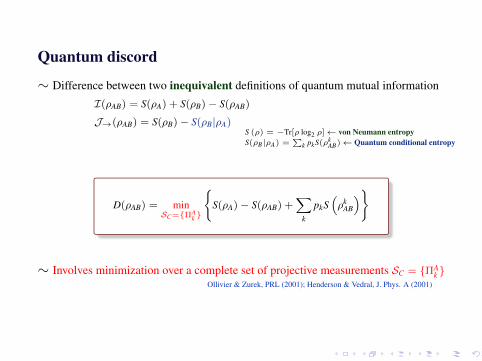
Quantum discord
∼ Difference between two inequivalent definitions of quantum mutual information
I(ρAB) = S(ρA) + S(ρB)− S(ρAB)
J→(ρAB) = S(ρB)− S(ρB|ρA)S (ρ) = −Tr[ρ log2 ρ]← von Neumann entropyS(ρB|ρA) =
∑k pkS(ρk
AB)← Quantum conditional entropy
D(ρAB) = minSC={ΠA
k }
{S(ρA)− S(ρAB) +
∑k
pkS(ρk
AB
)}
∼ Involves minimization over a complete set of projective measurements SC = {ΠAk }
Ollivier & Zurek, PRL (2001); Henderson & Vedral, J. Phys. A (2001)

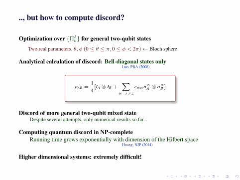
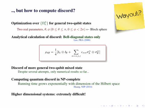
.., but how to compute discord?
Optimization over {ΠAk } for general two-qubit states
Two real parameters, θ, φ (0 ≤ θ ≤ π, 0 ≤ φ < 2π)← Bloch sphere
Analytical calculation of discord: Bell-diagonal states onlyLuo, PRA (2008)
ρAB =14
[IA ⊗ IB +∑
α=x,y,z
cαασαA ⊗ σαB ]
Discord of more general two-qubit mixed stateDespite several attempts, only numerical results so far...
Computing quantum discord in NP-completeRunning time grows exponentially with dimension of the Hilbert space
Huang, NJP (2014)
Higher dimensional systems: extremely difficult!
How about a constrained optimization?
Restriction over the set of measurement: “Earmarked” setSE ⊆ SC
Dc = minSE
[I(ρAB)− J→(ρAB)] D = minSC
[I(ρAB)− J→(ρAB)]
n sets of projection measurements in SE
n→∞ may/may not imply SE → SC, i.e., Dc → D
Dc ≥ D −→ εn = Dc − D ←− “Voluntary error”
εn = 0 ←− “Exceptional states”

How about a constrained optimization?Restriction over the set of measurement: “Earmarked” set
SE ⊆ SC
Dc = minSE
[I(ρAB)− J→(ρAB)]
D = minSC
[I(ρAB)− J→(ρAB)]
n sets of projection measurements in SE
n→∞ may/may not imply SE → SC, i.e., Dc → D
Dc ≥ D −→ εn = Dc − D ←− “Voluntary error”
εn = 0 ←− “Exceptional states”
How about a constrained optimization?Restriction over the set of measurement: “Earmarked” set
SE ⊆ SC
Dc = minSE
[I(ρAB)− J→(ρAB)] D = minSC
[I(ρAB)− J→(ρAB)]
n sets of projection measurements in SE
n→∞ may/may not imply SE → SC, i.e., Dc → D
Dc ≥ D −→ εn = Dc − D ←− “Voluntary error”
εn = 0 ←− “Exceptional states”

n points
εrn =
∫εr
nPrn(εr
n)dεrn
εr∞← “Average asymptotic error”
Two-qubit mixed states of different ranks, r
εrn = εr
∞ + κn−τ
For r = 2τ ≈ 1.92κ ≈ 0.177εr=2∞ ≈ 0.121
For r = 4τ ≈ 1.93κ ≈ 0.145εr=4∞ ≈ 0.078
Better for higher rank
0
0.02
0.04
0.06
0.08
0.1
0.12
0.14
0.16
0.18
5 10 15 20 25 30 35 40 45 50
– εr=
2n −
– ε
r=
2∞
n
QD-numerical
QD-fitted
10-4
10-3
10-2
10-1
2 5 10 20 50 1
n =∑n2
i=1 ni1
0.04
0.06
0.08
0.1
0.12
0.14
5 10 15 20 25 30
– εnr
n2
Rank 2
Rank 3, NPPT
Rank 3, PPT
Rank 4, NPPT
Rank 4, PPT
n1 = 10
n = n1 × n2
for QD
2 4 6 8 10 12 14
n1
2
4
6
8
10
12
14
n2
0
0.05
0.1
0.15
0.2
0.25
A
Rank 2
(a)
2 4 6 8 10 12 14
n1
2
4
6
8
10
12
14
n2
0
0.02
0.04
0.06
0.08
0.1
0.12
0.14
0.16
0.18
A
Rank 4, NPPT
(b)
2 4 6 8 10 12 14
n1
2
4
6
8
10
12
14
n2
0
0.02
0.04
0.06
0.08
0.1
0.12
A
Rank 4, PPT
εrn ≤ 10−3 outside boundary
Faster for higher rank, PPT states

Triad
n = 3
-1-0.5
0 0.5
1 0
0.5 1
1.5 2
2.5 3
0
1
2
3
4
5
6
7
8
9
P(fθ, φ)
fθ
φ
P(fθ, φ)
fθ = cos θ
ρAB =14
[IA ⊗ IB +∑
α=x,y,z
cαασαA ⊗ σαB +∑
α=x,y,z
cAασ
αA ⊗ IB +
∑β=x,y,z
cBβ IA ⊗ σβB ]

Triad
n = 3
-1-0.5
0 0.5
1 0
0.5 1
1.5 2
2.5 3
0
1
2
3
4
5
6
7
8
9
P(fθ, φ)
fθ
φ
P(fθ, φ)
fθ = cos θ
ρAB =14
[IA ⊗ IB +∑
α=x,y,z
cαασαA ⊗ σαB +∑
α=x,y,z
cAασ
αA ⊗ IB +
∑β=x,y,z
cBβ IA ⊗ σβB ]

Triad
n = 3
-1-0.5
0 0.5
1 0
0.5 1
1.5 2
2.5 3
0
1
2
3
4
5
6
7
8
9
P(fθ, φ)
fθ
φ
P(fθ, φ)
fθ = cos θ
ρAB =14
[IA ⊗ IB +∑
α=x,y,z
cαασαA ⊗ σαB +∑
α=x,y,z
cAασ
αA ⊗ IB +
∑β=x,y,z
cBβ IA ⊗ σβB ]
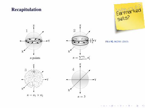
Recapitulation
n points n =∑n2
i=1 ni1
PRA 92, 062301 (2015)
n = n1 × n2 n = 3
Only discord?

Recapitulation
n points n =∑n2
i=1 ni1
PRA 92, 062301 (2015)
n = n1 × n2 n = 3
Only discord?

How about other correlation measures?
Quantum work deficit: W(ρAB) = min{ΠA
k }
[S(∑
k pkρkAB)− S(ρAB)
]Horodecki et. al., PRA (2005)
for QD
2 4 6 8 10 12 14
n1
2
4
6
8
10
12
14
n2
0
0.05
0.1
0.15
0.2
0.25
A
Rank 2
(a)
for QWD
2 4 6 8 10 12 14
n1
2
4
6
8
10
12
14
n2
0
0.05
0.1
0.15
0.2
0.25
0.3
0.35
A
Rank 2
(d)
2 4 6 8 10 12 14
n1
2
4
6
8
10
12
14
n2
0
0.02
0.04
0.06
0.08
0.1
0.12
0.14
0.16
0.18
A
Rank 4, NPPT
(b)
2 4 6 8 10 12 14
n1
2
4
6
8
10
12
14
n2
0 0.02 0.04 0.06 0.08 0.1 0.12 0.14 0.16 0.18 0.2
A
Rank 4, NPPT
(e)
2 4 6 8 10 12 14
n1
2
4
6
8
10
12
14
n2
0
0.02
0.04
0.06
0.08
0.1
0.12
A
Rank 4, PPT
2 4 6 8 10 12 14
n1
2
4
6
8
10
12
14
n2
0
0.02
0.04
0.06
0.08
0.1
0.12
0.14
0.16
A
Rank 4, PPT
Hierarchy in correlation measures

How about other correlation measures?Quantum work deficit: W(ρAB) = min
{ΠAk }
[S(∑
k pkρkAB)− S(ρAB)
]Horodecki et. al., PRA (2005)
for QD
2 4 6 8 10 12 14
n1
2
4
6
8
10
12
14
n2
0
0.05
0.1
0.15
0.2
0.25
A
Rank 2
(a)
for QWD
2 4 6 8 10 12 14
n1
2
4
6
8
10
12
14
n2
0
0.05
0.1
0.15
0.2
0.25
0.3
0.35
A
Rank 2
(d)
2 4 6 8 10 12 14
n1
2
4
6
8
10
12
14
n2
0
0.02
0.04
0.06
0.08
0.1
0.12
0.14
0.16
0.18
A
Rank 4, NPPT
(b)
2 4 6 8 10 12 14
n1
2
4
6
8
10
12
14
n2
0 0.02 0.04 0.06 0.08 0.1 0.12 0.14 0.16 0.18 0.2
A
Rank 4, NPPT
(e)
2 4 6 8 10 12 14
n1
2
4
6
8
10
12
14
n2
0
0.02
0.04
0.06
0.08
0.1
0.12
A
Rank 4, PPT
2 4 6 8 10 12 14
n1
2
4
6
8
10
12
14
n2
0
0.02
0.04
0.06
0.08
0.1
0.12
0.14
0.16
A
Rank 4, PPT
Hierarchy in correlation measures

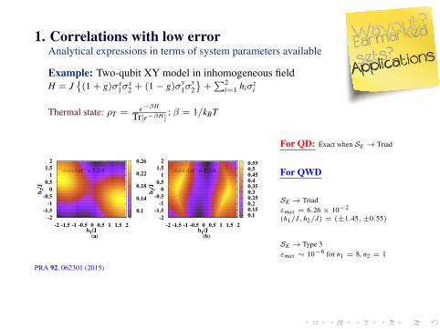
1. Correlations with low errorAnalytical expressions in terms of system parameters available
Example: Two-qubit XY model in inhomogeneous fieldH = J
{(1 + g)σx
1σx2 + (1− g)σy
1σy2
}+∑2
i=1 hiσzi
Thermal state: ρT = e−βH
Tr[e−βH ]; β = 1/kBT
(a)
"data.dat" u 1:2:4
-2 -1.5 -1 -0.5 0 0.5 1 1.5 2h1/J
-2
-1.5
-1
-0.5
0
0.5
1
1.5
2
h2/J
0.1
0.14
0.18
0.22
0.26
(b)
"data.dat" u 1:2:6
-2 -1.5 -1 -0.5 0 0.5 1 1.5 2h1/J
-2
-1.5
-1
-0.5
0
0.5
1
1.5
2
h2/J
0.1 0.15 0.2 0.25 0.3 0.35 0.4 0.45 0.5 0.55
For QD: Exact when SE→ Triad
For QWD
SE→ Triadεmax = 6.26× 10⁻²
(h1/J, h2/J) = (±1.45,±0.55)
SE→ Type 3εmax ∼ 10−6 for n1 = 8, n2 = 1
PRA 92, 062301 (2015)

.., but how to compute discord?
Optimization over {ΠAk } for general two-qubit states
Two real parameters, θ, φ (0 ≤ θ ≤ π, 0 ≤ φ < 2π)← Bloch sphere
Analytical calculation of discord: Bell-diagonal states onlyLuo, PRA (2008)
ρAB =14
[IA ⊗ IB +∑
α=x,y,z
cαασαA ⊗ σαB ]
Discord of more general two-qubit mixed stateDespite several attempts, only numerical results so far...
Computing quantum discord in NP-completeRunning time grows exponentially with dimension of the Hilbert space
Huang, NJP (2014)
Higher dimensional systems: extremely difficult!

2. Investigating decoherence“Freezing phenomena”
Canonical initial states under local quantum channels
Example: ρ̃AB under bit-flip channel
ρ̃AB =14
[IA ⊗ IB +∑
α=x,y,z
cαασαA ⊗ σαB + (cAx σ
xA ⊗ IB + cB
x IA ⊗ σxB)]
Necessary & sufficient initial conditions for freezing can be determined
PRA 91, 062119 (2015)

3. Higher dimensional systemsStates with positive partial transposition
Example:
%α =27|ψ〉〈ψ|+ α
7%+ +
5− α7
%−
%+ = (|01〉〈01| + |12〉〈12| + |20〉〈20|)/3%− = (|10〉〈10| + |21〉〈21| + |02〉〈02|)/3|ψ〉 = 1√
3
∑2i=0 |ii〉
0 ≤ α ≤ 5
Bound entangled: 1 < α ≤ 2, 3 < α ≤ 4Separable: 2 ≤ α ≤ 3Distillable: 0 < α ≤ 1, 4 < α ≤ 5
0.34
0.36
0.38
0.4
0.42
0.44
0.46
0 1 2 3 4 5
QD
α
DcDa
0×100
2×10⁻³
4×10⁻³
6×10⁻³
8×10⁻³
1×10⁻²
0 1 2 3 4 5
ε
α
PRA 92, 062301 (2015)

In a nutshell...
• Constrained quantum correlations
• Analytical formula with low error
• Applications in many-body physics, decoherence, higher dimensional systems
• Applicable to other scenarios involving optimization


![HOLOGRAPHY, QUANTUM GEOMETRY, AND QUANTUM INFORMATION THEORY · The emerging fields of quantum computation [22], quantum communication and quantum cryptography [23], quantum dense](https://img.dokumen.tips/doc/110x75/5ec76f6b603b2e345706bd5a/holography-quantum-geometry-and-quantum-information-theory-the-emerging-fields.jpg)