Embed Size (px)
Citation preview
SANDIA REPORTSAND2005-6864Unlimited ReleasePrinted November 2005
Robust Large-scale Parallel NonlinearSolvers for Simulations
Brett W. Bader, Roger P. Pawlowski, and Tamara G. Kolda
Prepared bySandia National LaboratoriesAlbuquerque, New Mexico 87185 and Livermore, California 94550
Sandia is a multiprogram laboratory operated by Sandia Corporation,a Lockheed Martin Company, for the United States Department of Energy’sNational Nuclear Security Administration under Contract DE-AC04-94-AL85000.
Approved for public release; further dissemination unlimited.

Issued by Sandia National Laboratories, operated for the United States Department ofEnergy by Sandia Corporation.
NOTICE: This report was prepared as an account of work sponsored by an agency ofthe United States Government. Neither the United States Government, nor any agencythereof, nor any of their employees, nor any of their contractors, subcontractors, or theiremployees, make any warranty, express or implied, or assume any legal liability or re-sponsibility for the accuracy, completeness, or usefulness of any information, appara-tus, product, or process disclosed, or represent that its use would not infringe privatelyowned rights. Reference herein to any specific commercial product, process, or serviceby trade name, trademark, manufacturer, or otherwise, does not necessarily constituteor imply its endorsement, recommendation, or favoring by the United States Govern-ment, any agency thereof, or any of their contractors or subcontractors. The views andopinions expressed herein do not necessarily state or reflect those of the United StatesGovernment, any agency thereof, or any of their contractors.
Printed in the United States of America. This report has been reproduced directly fromthe best available copy.
Available to DOE and DOE contractors fromU.S. Department of EnergyOffice of Scientific and Technical InformationP.O. Box 62Oak Ridge, TN 37831
Telephone: (865) 576-8401Facsimile: (865) 576-5728E-Mail: [email protected] ordering: http://www.doe.gov/bridge
Available to the public fromU.S. Department of CommerceNational Technical Information Service5285 Port Royal RdSpringfield, VA 22161
Telephone: (800) 553-6847Facsimile: (703) 605-6900E-Mail: [email protected] ordering: http://www.ntis.gov/ordering.htm
ii
SAND2005-6864Unlimited Release
PrintedNovember 2005
Robust Large-scale Parallel Nonlinear Solvers forSimulations
Brett W. Bader and Roger P. PawlowskiApplied Computational Methods, Dept. 1416
Sandia National LaboratoriesP.O. Box 5800, MS-0316
Albuquerque, NM 87185-0316
Tamara KoldaComputational Sciences and Math, Dept. 8962
Sandia National LaboratoriesP.O. Box 969, MS-9159
Livermore, CA 94551-9159
iii
Abstract
This report documents research to develop robust and efficient solution techniques forsolving large-scale systems of nonlinear equations. The most widely used method for solv-ing systems of nonlinear equations is Newton’s method. While much research has beendevoted to augmenting Newton-based solvers (usually with globalization techniques), littlehas been devoted to exploring the application of different models. Our research has beendirected at evaluating techniques using different models than Newton’s method: a lowerorder model, Broyden’s method, and a higher order model, the tensor method. We havedeveloped large-scale versions of each of these models and have demonstrated their use inimportant applications at Sandia.
Broyden’s method replaces the Jacobian with an approximation, allowing codes thatcannot evaluate a Jacobian or have an inaccurate Jacobian to converge to a solution. Limited-memory methods, which have been successful in optimization, allow us to extend thisapproach to large-scale problems. We compare the robustness and efficiency of New-ton’s method, modified Newton’s method, Jacobian-free Newton-Krylov method, and ourlimited-memory Broyden method. Comparisons are carried out for large-scale applicationsof fluid flow simulations and electronic circuit simulations. Results show that, in caseswhere the Jacobian was inaccurate or could not be computed, Broyden’s method convergedin some cases where Newton’s method failed to converge. We identify conditions whereBroyden’s method can be more efficient than Newton’s method.
We also present modifications to a large-scale tensor method, originally proposed byBouaricha, for greater efficiency, better robustness, and wider applicability. Tensor meth-ods are an alternative to Newton-based methods and are based on computing a step based ona local quadratic model rather than a linear model. The advantage of Bouaricha’s methodis that it can use any existing linear solver, which makes it simple to write and easilyportable. However, the method usually takes twice as long to solve as Newton-GMRESon general problems because it solves two linear systems at each iteration. In this paper,we discuss modifications to Bouaricha’s method for a practical implementation, includinga special globalization technique and other modifications for greater efficiency. We presentnumerical results showing computational advantages over Newton-GMRES on some real-istic problems.
We further discuss a new approach for dealing with singular (or ill-conditioned) ma-trices. In particular, we modify an algorithm for identifying a turning point so that anincreasingly ill-conditioned Jacobian does not prevent convergence.
iv
Contents
1 Introduction 1
1.1 Broyden’s Method for Nonlinear Problems . . . . . . . . . . . . . . . . . . . . . . . . . .2
1.2 Tensor Methods for Nonlinear Problems . . . . . . . . . . . . . . . . . . . . . . . . . . . .3
1.3 Tensor Methods for Bifurcation Tracking . . . . . . . . . . . . . . . . . . . . . . . . . . .4
1.4 Organization and Notation . . . . . . . . . . . . . . . . . . . . . . . . . . . . . . . . . . . . . . .4
2 Broyden Methods 5
2.1 Theory . . . . . . . . . . . . . . . . . . . . . . . . . . . . . . . . . . . . . . . . . . . . . . . . . . . . . .5
2.1.1 The Choice ofB0 for Broyden’s Method . . . . . . . . . . . . . . . . . . . . . 7
2.1.2 An Implicit Representation of the Broyden matrix . . . . . . . . . . . . . .8
2.1.3 A More Efficient Implicit Representation of the Broyden Matrix . .9
2.2 Implementation Issues . . . . . . . . . . . . . . . . . . . . . . . . . . . . . . . . . . . . . . . . . .11
2.3 Results . . . . . . . . . . . . . . . . . . . . . . . . . . . . . . . . . . . . . . . . . . . . . . . . . . . . . .12
2.3.1 Counterflow Jet Reactor . . . . . . . . . . . . . . . . . . . . . . . . . . . . . . . . . .12
2.3.1.1 Robustness Under Inaccurate Jacobians . . . . . . . . . . . . . .14
2.3.1.2 Efficiency Comparisons . . . . . . . . . . . . . . . . . . . . . . . . . .17
2.3.2 Thermal Convection . . . . . . . . . . . . . . . . . . . . . . . . . . . . . . . . . . . . .19
2.3.3 Circuit Simulation . . . . . . . . . . . . . . . . . . . . . . . . . . . . . . . . . . . . . . .21
2.4 Discussion . . . . . . . . . . . . . . . . . . . . . . . . . . . . . . . . . . . . . . . . . . . . . . . . . . .23
v

3 Tensor Methods 25
3.1 Introduction . . . . . . . . . . . . . . . . . . . . . . . . . . . . . . . . . . . . . . . . . . . . . . . . . .25
3.2 Background on Tensor Methods . . . . . . . . . . . . . . . . . . . . . . . . . . . . . . . . . .27
3.2.1 Tensor Methods . . . . . . . . . . . . . . . . . . . . . . . . . . . . . . . . . . . . . . . . .27
3.2.1.1 Method of Orthogonal Transformations . . . . . . . . . . . . . .28
3.2.1.2 Reduction Method . . . . . . . . . . . . . . . . . . . . . . . . . . . . . . .29
3.2.2 Global Strategies . . . . . . . . . . . . . . . . . . . . . . . . . . . . . . . . . . . . . . . .30
3.3 Review of Large-scale Methods . . . . . . . . . . . . . . . . . . . . . . . . . . . . . . . . . . .31
3.3.1 Newton-Krylov Methods . . . . . . . . . . . . . . . . . . . . . . . . . . . . . . . . . .31
3.3.2 Bouaricha’s Method . . . . . . . . . . . . . . . . . . . . . . . . . . . . . . . . . . . . .32
3.3.3 Tensor-GMRES Method . . . . . . . . . . . . . . . . . . . . . . . . . . . . . . . . . .35
3.3.4 Tensor-Krylov Methods . . . . . . . . . . . . . . . . . . . . . . . . . . . . . . . . . .37
3.3.4.1 Block-3 Local Solver . . . . . . . . . . . . . . . . . . . . . . . . . . . .38
3.3.4.2 Tensor-Krylov Nonlinear Solver . . . . . . . . . . . . . . . . . . . .41
3.3.4.3 Global Strategy and Step Selection . . . . . . . . . . . . . . . . . .41
3.4 Modified Bouaricha Method . . . . . . . . . . . . . . . . . . . . . . . . . . . . . . . . . . . . .42
3.5 Computational Results . . . . . . . . . . . . . . . . . . . . . . . . . . . . . . . . . . . . . . . . . .45
3.5.1 Test Results on Fluid Flow Benchmark Problems . . . . . . . . . . . . . .45
3.5.1.1 Thermal Convection Problem . . . . . . . . . . . . . . . . . . . . . .48
3.5.1.2 Backward-facing Step Problem . . . . . . . . . . . . . . . . . . . .50
3.5.2 Test Results on a Circuit Simulation Problem . . . . . . . . . . . . . . . . . .53
3.6 Discussion . . . . . . . . . . . . . . . . . . . . . . . . . . . . . . . . . . . . . . . . . . . . . . . . . . .54
4 Turning Point Algorithm 58
4.1 Singular and Ill-conditioned Jacobians . . . . . . . . . . . . . . . . . . . . . . . . . . . . .58
4.1.1 Tensor Methods . . . . . . . . . . . . . . . . . . . . . . . . . . . . . . . . . . . . . . . . .58
vi
4.1.2 General Linear Systems . . . . . . . . . . . . . . . . . . . . . . . . . . . . . . . . . .61
4.2 Turning Point Identification . . . . . . . . . . . . . . . . . . . . . . . . . . . . . . . . . . . . . .62
4.2.1 Bordered Algorithm . . . . . . . . . . . . . . . . . . . . . . . . . . . . . . . . . . . . .63
4.2.2 Modified Bordered Algorithm . . . . . . . . . . . . . . . . . . . . . . . . . . . . . .64
4.3 Computational Results . . . . . . . . . . . . . . . . . . . . . . . . . . . . . . . . . . . . . . . . . .65
4.4 Discussion . . . . . . . . . . . . . . . . . . . . . . . . . . . . . . . . . . . . . . . . . . . . . . . . . . .67
5 Summary 69
References 76
vii

viii

List of Figures
2.1 Streamlines for the flow pattern in a CJR. Reynolds number is 10. . . . . . . . .13
2.2 Plot of the residual norm as a function of nonlinear iteration number. . . . . .16
2.3 Thermal convection problem. Color contour plot of temperature with stream-lines at Ra=10E5 . . . . . . . . . . . . . . . . . . . . . . . . . . . . . . . . . . . . . . . . . . . . . .21
3.1 Thermal convection problem: Comparison of tensor methods . . . . . . . . . . .49
3.2 Thermal convection problem: Modified Bouaricha method . . . . . . . . . . . . .50
3.3 Thermal convection problem: Modified Bouaricha method (8 processors) . .51
3.4 Backward-facing step problem: Comparison of tensor methods . . . . . . . . . .52
3.5 Backward-facing step problem: Modified Bouaricha method . . . . . . . . . . . .53
3.6 Comparator circuit: Comparison of methods (nonlinear iterations) . . . . . . .55
3.7 Comparator circuit: Comparison of methods (time) . . . . . . . . . . . . . . . . . . .56
4.1 Comparison of turning point methods (residual norm) . . . . . . . . . . . . . . . . .67
4.2 Comparison of turning point methods (linear iterations) . . . . . . . . . . . . . . . .68
ix

x

List of Tables
2.1 A comparison of robust methods under inaccurate Jacobians. . . . . . . . . . . .17
2.2 Steady-state performance characteristics. . . . . . . . . . . . . . . . . . . . . . . . . . . .18
2.3 Transient performance characteristics. . . . . . . . . . . . . . . . . . . . . . . . . . . . . . .19
2.4 Transient thermal convection in a box. . . . . . . . . . . . . . . . . . . . . . . . . . . . . .20
2.5 Performance comparison for various circuits using the Xyce circuit simulator.22
xi

Chapter 1
Introduction
This report describes two classes of methods (and their extensions) for solving the nonlinearequations problem
givenF : Rn→ Rn, find x∗ ∈ Rn such thatF(x∗) = 0, (1.1)
where it is assumed thatF(x) is at least once continuously differentiable. Large-scalesystems of nonlinear equations defined by (1.1) arise in the simulation of many physicalphenomena at Sandia, including systems produced by finite-difference or finite-elementdiscretizations of boundary value problems for ordinary and partial differential equations.Typical examples include reacting flows, compressible flows, solid mechanics, device sim-ulation, and circuit simulation.
Newton-based strategies are the most widely used methods for solving systems ofnonlinear equations. While much research has been devoted to improving Newton-basedsolvers (usually with globalization techniques) [19, 38], little has been devoted to exploringthe applicability of different underlying models, such as Broyden’s method [57] and tensormethods [13]. Our research focuses on these alternate methods and investigates their per-formance on challenging problems. We present modifications to the basic algorithms thatresult in better performance, increased robustness, and greater ease-of-use.
Newton’s method for solving (1.1) is based on creating a linear local modelMN(xk+d)of the functionF(x) around the current iteratexk ∈ Rn:
MN(xk +d) = F(xk)+J(xk)d, (1.2)
whered ∈ Rn is the step andJ(xk) ∈ Rn×n is the current Jacobian matrix, which is definedas the derivative of the residual equations with respect to the unknowns, i.e.,
Ji j =∂Fi
∂x j.
A root of the local model (1.2) provides the Newton step
dN =−J(xk)−1F(xk),
1

which is used to reach the next trial point. Thus, Newton’s method is defined whenJk isnonsingular, and consists of updating the current point with the Newton step,
xk+1 = xk +dN. (1.3)
Because the sequence of iterates based upon (1.3) is not guaranteed to converge, a techniquefor modifying the step to ensure global convergence is used frequently. The two mostcommon choices of globalization schemes are a line search procedure (which scalesdN bya fractional value) or a trust region algorithm (which chooses an optimal direction to theextent that the local model is trusted); see, e.g., [19, 45].
Methods that use direct linear solvers are impractical on large-scale problems becauseof the high linear algebra costs and large memory requirements. Thus, most practical ap-proaches for solving large problems involve using an iterative method to approximatelysolve a local linear model using the Jacobian and then using the “inexact” step producedby the approximate solution. These methods are called “inexact” Newton methods [18].Successively better approximations at each iteration preserve the rapid convergence behav-ior of Newton’s method when nearing the solution. The computational savings reflected inthis less expensive linear solve is usually partially offset with more outer iterations, but theoverall savings is significant on large-scale problems.
Overall, Newton-based algorithms have many appealing properties such as robustness,scale invariance, and, most importantly, quadratic convergence. While Newton’s methodis usually the de facto standard, it is not always the best choice. This report discusses twoalternate strategies.
1.1 Broyden’s Method for Nonlinear Problems
In some cases, the derivative information required for a Newton-based solve is either un-available or cannot be calculated efficiently. In these cases, alternate strategies can be moreeconomical in terms of both implementation and execution costs.
Broyden’s method [13] is an alternative to Newton’s method that does not require anaccurate Jacobian matrix. Broyden’s method for solving (1.1) is based on creating an ap-proximate linear local modelMB(xk + d) of the functionF(x) around the current iteratexk ∈ Rn:
MB(xk +d) = F(xk)+Bkd,
whereBk ∈ Rn×n is an approximation to the Jacobian composed of a sequence of secantapproximations. Each secant approximation adds a rank-1 matrix to the Jacobian approxi-mation so that the local model interpolates the function value at past iterates. In this way,approximate derivative information in the direction of the previous steps is included in thelocal model.
Since the Jacobian is approximated using information generated in previous iterates, theapplication need only supplyB0, the initial approximation to the Jacobian. This matrix can
2
be as simple as the identity matrix, thus removing any requirement of a Jacobian evaluation.The closerB0 approximates the Jacobian, the more efficient Broyden’s method becomes.Due to the simple nature of the approximation matrix, Broyden’s method requires very littlecomputation time to perform a step, which makes it suitable for solving some large-scaleproblems.
The primary goal of our research with Broyden’s method was to evaluate its perfor-mance and determine cases where this technology should be employed. We compare alimited-memory version of Broyden’s method, based on [38], to various Newton-basedstrategies on a limited set of test problems.
1.2 Tensor Methods for Nonlinear Problems
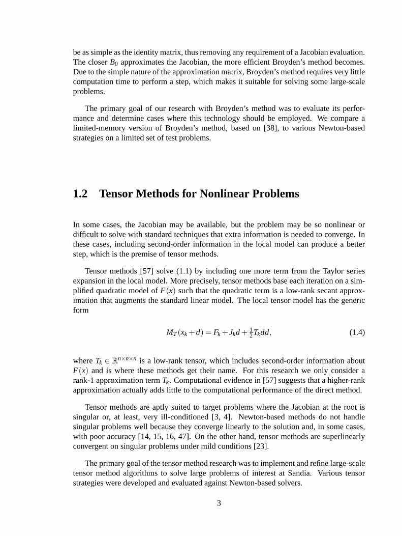
In some cases, the Jacobian may be available, but the problem may be so nonlinear ordifficult to solve with standard techniques that extra information is needed to converge. Inthese cases, including second-order information in the local model can produce a betterstep, which is the premise of tensor methods.
Tensor methods [57] solve (1.1) by including one more term from the Taylor seriesexpansion in the local model. More precisely, tensor methods base each iteration on a sim-plified quadratic model ofF(x) such that the quadratic term is a low-rank secant approx-imation that augments the standard linear model. The local tensor model has the genericform
MT(xk +d) = Fk +Jkd+ 12Tkdd, (1.4)
whereTk ∈ Rn×n×n is a low-rank tensor, which includes second-order information aboutF(x) and is where these methods get their name. For this research we only consider arank-1 approximation termTk. Computational evidence in [57] suggests that a higher-rankapproximation actually adds little to the computational performance of the direct method.
Tensor methods are aptly suited to target problems where the Jacobian at the root issingular or, at least, very ill-conditioned [3, 4]. Newton-based methods do not handlesingular problems well because they converge linearly to the solution and, in some cases,with poor accuracy [14, 15, 16, 47]. On the other hand, tensor methods are superlinearlyconvergent on singular problems under mild conditions [23].
The primary goal of the tensor method research was to implement and refine large-scaletensor method algorithms to solve large problems of interest at Sandia. Various tensorstrategies were developed and evaluated against Newton-based solvers.
3
1.3 Tensor Methods for Bifurcation Tracking
A final aspect of this research dealt with turning point identification algorithms. Becausetensor methods have a faster rate of convergence than Newton’s method on singular prob-lems [23], our research focused on applying this technology to the bifurcation trackingalgorithms in LOCA, particularly the turning point identification algorithm. LOCA uses aspecial technique called a bordering algorithm for solving this nonlinear problem by solv-ing four intermediate subproblems involving the Jacobian matrix [55]. A linear combina-tion of these four subproblem solutions provides the Newton step for the overall problem.However, because the algorithm is driving the Jacobian to a singularity, the four subprob-lems are increasingly difficult to solve and less accurate, which makes the resultant stepless accurate and eventually unusable due to floating point round-off errors.
We investigated applying tensor methods to the bordered algorithm for turning pointidentification. Our research showed that a straightforward applications of tensor methods tothe overall nonlinear problem did not appreciably improve the performance of the turningpoint algorithm. Nonetheless, we were able to improve the stability and accuracy of theturning point algorithm with a novel approach to solving ill-conditioned linear systemsusing an idea from tensor methods.
1.4 Organization and Notation
The organization of this report is broken into three main chapters, following the three dis-tinct topics in our research. Each chapter is intended to be a stand-alone paper. Chapter 2presents our research on Broyden’s method. Chapter 3 discusses our research on tensormethods. Chapter 4 discusses the tensor method techniques applied to bifurcation identifi-cation algorithms. Each chapter contains its own summary and discussion, and Chapter 5provides a broad summary of the overall project.
Throughout this report, the subscriptk refers to the iteration number of the nonlineariteration sequence. We denote the JacobianF ′(x) by J(x) and frequently abbreviateJ(xk)asJk andF(xk) asFk. In keeping with the notation of Taylor series approximations for thevalueF(xk + d), we denote local models of a function about a pointxk asM(xk + d) andhave included a subscriptN, B, orT onM to specify the Newton, Broyden, or tensor model,respectively. In addition, the respective steps that solve these local models are denoteddN,dB, anddT .
4

Chapter 2
Broyden Methods
In this chapter, we describe and evaluate Broyden’s method for the solution of nonlinearequations, an alternative to Newton-based methods that does not require Jacobian informa-tion (but will make efficient use of any approximation to the Jacobian that is provided). Thischapter presents Broyden’s method and compares the algorithm with Newton’s method.Examples from application codes used at Sandia are shown. The results demonstrate situ-ations where Broyden’s method is preferable to Newton’s method.
2.1 Theory
The most prevalent strategy for solving nonlinear equations is to apply Newton’s methodto iteratively solve a local linear model until convergence [19]. The local linear model isdefined as:
M(xk +d) = Fk +Jk d, (2.1)
wherek is the iterate number,xk is the current solution iterate (the approximation to thesolution at iterationk), Jk ∈ IRn×n is the Jacobian matrix evaluated atxk, andFk = F(xk) isthe residual evaluated atxk. The Jacobian matrix is defined as the derivative of the residualequations with respect to the unknowns, i.e.,
Ji j =∂Fi
∂x j. (2.2)
The next iterate is defined asxk+1 = xk +dk,
wheredk is the solution to 2.1.
Some form of globalization may be needed to guarantee convergence. If a line searchis used for globalization, then
xk+1 = xk +λkdk,
5
whereλk is the line search parameter. The iterations progress until the approximate solutionsatisfies some convergence criteria. If a line search is used for globalization, the algorithmis as follows:
Algorithm GN [20]: Globalized Newton Method
LET x0 BE GIVEN.
FOR k = 0, 1, . . . (UNTIL CONVERGENCE) DO:
SOLVE: Jkdk =−Fk FOR dk
COMPUTE: λk VIA A LINE SEARCH
SET xk+1 = xk +λkdk.
If there is no line search, thenλk = 1 for all k.
The iteration sequence above can be rewritten as follows:
xk+1 = xk−λkJ−1k Fk (2.3)
Each nonlinear iteration requires solving a linear system. Difficulties arise not only ininverting or preconditioning the Jacobian, but also in computing the Jacobian. In fact, it isnot always possible to compute the Jacobian directly because of the type of discretizationscheme or because of discontinuities in derivative evaluations (e.g., due to table look-upsfor material properties, third-party library functions, etc.). For example, the compressibleflow code Premo [1] uses a 2nd order accurate finite volume scheme with Roe flux limitingthat makes evaluating the Jacobian extremely complex and error-prone. Instead, coloredfinite difference techniques [25] and automatic differentiation [30] are used to evaluatethe Jacobian. Finite differencing can be slow, especially if the connectivity graph is notsupplied by the user. Additionally, the Jacobian may be inexact due to residuals that involvediscontinuous derivatives (i.e., table look-ups) or difficult terms being ignored. Automaticdifferentiation is a promising technology for evaluating the Jacobian, but no universal toolhas been developed. In some cases, Jacobians for FORTRAN and C code can be generatedusing source transformation software such as ADIFOR [7] and ADIC [8]. C++, on theother hand, requires an invasive templating of the scalar type in all residual fill algorithms.This can be difficult to use especially when programming languages are mixed due to thirdparty libraries.
Instead of using a linear model as in 2.3, we propose to use an alternative model intro-duced by Broyden [13]. The iteration sequence in 2.3 is then replaced by:
xk+1 = xk−λkB−1k Fk (2.4)
whereBk ≈ J(xk) is an approximation to the Jacobian based on a least-change secant up-date. Our implementation follows the limited-memory Broyden algorithm in Kelley [37,§8,3,2].
6
Recall that thesearch directionis denoted bydk =−B−1k Fk. Let sk denote thekth step;
i.e.,sk = xk+1−xk =−λkB
−1k Fk = λkdk. (2.5)
If no line search is used (so thatλk = 1 for all k), thensk = dk.
It is interesting to note that the use of a line search can be problematic sincedk is notguaranteed to be a descent direction. Kelley [38] recommends that if a line search withBroyden’s method fails, one should look to better preconditioning strategies or move to aNewton-Krylov scheme. In our computations, if the Broyden method fails during a linesearch, we recompute the Jacobian estimate and attempt another solve.
The Broyden update is asecant update, i.e., it obeys the secant condition:
Bk+1sk = yk, (2.6)
whereyk = Fk+1−Fk. The Broyden update represents the least change from the previousmatrix,Bk, that satisfies the secant condition. It is defined as
Bk+1 = Bk +(yk−Bksk)sT
k
‖sk‖22. (2.7)
A more convenient expression forBk can be derived by observing that
yk−Bksk = (Fk+1−Fk)+λkFk = Fk+1− (1−λk)Fk, (2.8)
and so we can rewriteBk as
Bk+1 = Bk +(Fk+1− (1−λk)Fk)sT
k
‖sk‖22. (2.9)
This recursive formula means thatBk can be formed implicitly, as we discuss in more detailin the sections that follow. Note that the updates are based on the residual evaluations (i.e.,values ofF), and so there is no need to compute a Jacobian.
2.1.1 The Choice ofB0 for Broyden’s Method
The following is the analogue of Lemma 7.3.1 in [37]; here it is extended to the case witha line search parameter.
Lemma 2.1.1 Letxk,Bk be the Broyden sequence generated by(F,x0,B0), and letzk,Ckbe the Broyden sequence generated by(B−1
0 F,x0, I). Then
xk = zk and Bk = B0Ck. (2.10)
(We assume the step lengths,λk, are the same for each sequence.)
7
This is a proof by induction. The case fork = 0 is trivial. Assume the claim holds fork.Observe that,
xk+1 = xk−λkB−1k Fk
= zk−λk(B0Ck)−1Fk
= zk−λkC−1k (B−1
0 Fk)= zk+1,
and
Bk+1 = Bk +(Fk+1− (1−λk)Fk)sT
k
‖sk‖22
= B0Ck +B0
(B−1
0 Fk+1− (1−λk)B−10 Fk
)sTk
‖sk‖22= B0Ck+1.
Q.E.D.
An important consequence of this lemma is that we can assume thatB0 = I for all theanalysis that follows.
2.1.2 An Implicit Representation of the Broyden matrix
The Broyden matrix can be stored implicitly using only 2k vectors plusB0; see, e.g., Kelley[37] whose derivation is as follows.
We can express the Broyden update as a function of the previous iterate’s Broydenmatrix and a pair of vectors:
Bk+1 = Bk +ukvTk , (2.11)
where
uk =Fk+1− (1−λk)Fk
‖sk‖2and vk =
sk
‖sk‖2. (2.12)
We can now rearrange equation 2.11 into a more usable form that can be quite efficient.The Sherman-Woodbury-Morrison formula [27] says
Bk+1 =
(I −
(B−1k uk)vT
k
1+vkB−1k uk
)B−1
k . (2.13)
We define
wk =B−1
k uk
1+vkB−1k uk
=B−1
k (Fk+1− (1−λk)Fk)
‖sk‖2 +vTk B−1
k (Fk+1− (1−λk)Fk). (2.14)
8
Then
B−1k+1 = (I −wkv
Tk )B−1
k =k
∏j=0
(I −w jvTj ). (2.15)
Thus, the inverse of the Broyden matrix can be stored using only 2k vectors plus the initialmatrix inverseB−1
0 .
2.1.3 A More Efficient Implicit Representation of the Broyden Matrix
Kelley [37] observed that the Broyden matrix can be stored using onlyk+ 1 vectors. Hisderivation is as follows.
Define
zk = B−1k (Fk+1− (1−λk)Fk) and αk = ‖sk‖2 +vT
k zk+1, (2.16)
so that
wk =zk
αk. (2.17)
Then
dk+1 = −B−1k+1Fk+1
= −(I −wkv
Tk
)B−1
k Fk+1
= −(I −wkv
Tk
)(B−1
k Fk+1− (1−λk)B−1k Fk +(1−λk)B−1
k Fk
)= −
(I − zk
αkvT
k
)(zk +(1−λ−1
k )sk
)= −
(1−
vTk zk
αk−
(λ−1
k −1
αk
)vT
k sk
)zk− (λ−1
k −1)sk
= −
(1−
vTk zk +(λ−1
k −1)‖sk‖2αk
)zk− (λ−1
k −1)sk
= −
(1−
vTk zk +(λ−1
k −1)‖sk‖2 +λ−1k ‖sk‖2
αk+
λ−1k ‖sk‖2
αk
)zk− (λ−1
k −1)sk
= −λ−1k ‖sk‖2
zk
αk− (λ−1
k −1)sk
= −λ−1k ‖sk‖2wk− (λ−1
k −1)sk.
9
Solving forwk, we have
wk =−λk
‖sk‖2
(dk+1 +(1−λ−1
k )sk
)= −λk
dk+1
‖sk‖2+(1−λk)
sk
‖sk‖2
=−λk
λk+1
sk+1
‖sk‖2+(1−λk)
sk
‖sk‖2.
Substitutingwk in the expression fordk+1 yields
dk+1 = −B−1k+1Fk+1
= −(I −wkvTk )B−1
k Fk+1
= −(
I +λkdk+1sT
k
‖sk‖22− (1−λk)
sksTk
‖sk‖22
)B−1
k Fk+1
= −B−1k Fk+1−λk
sTk B−1
k Fk+1
‖sk‖22dk+1 +(1−λk)
sTk B−1
k Fk+1
‖sk‖22sk.
Solving fordk+1, we get
dk+1 =−B−1
k Fk+1 +(1−λk)sTk B−1
k Fk+1
‖sk‖22sk
1+λksTk B−1
k Fk+1
‖sk‖22
= −‖sk‖22B−1
k Fk+1 +(λk−1)sTk B−1
k Fk+1sk
‖sk‖22 +λksTk B−1
k Fk+1
=‖sk‖22 pk +(λk−1)sT
k pk sk
‖sk‖22−λksTk pk
wherepk =−BkFk+1. The value ofpk is calculated recursively as follows. Let
p0k =−Fk+1 and p j+1
k = (I −w jvTj )p j
k for j = 0, . . . ,k−1. (2.18)
Thenpk = pkk = B−1
k Fk+1. The formula forp j+1k can be rewritten as
p j+1k = p j
k +λ j
λ j+1
sTj p j
k
‖sj‖22sj+1 +(λ j −1)
sTj p j
k
‖sj‖22sj , (2.19)
for j = 0, . . . ,k−1.
The critical aspect in Broyden’s method is that, as the iterations ink progress, we buildup a set of rank-1 updates, and in combination with the initial Broyden matrix inverse,
10
B−10 , we get an estimate of the action of the current Jacobian without having to evaluate it
directly at each iteration. We are in effect implicitly storing the inverse of the Jacobian ateach iteration. This fact allows the Broyden method to be very efficient since we can reusethe factorization ofB0 for direct linear solves or we can reuse the preconditioner in the caseof iterative linear solves. Additionally, the Broyden method makes no assumptions on howto solve the inverse of the Broyden matrix. This can be critical in certain applications. Wewill comment more on this in section 2.3.1.1.
2.2 Implementation Issues
During the assessment of Broyden’s method, minor issues were found to have a criticalimpact on performance. The implementation had to be adjusted in order to address bothrobustness and efficiency issues. The key modification details are described in this section.
The first issue is the choice of the initial guess for the Broyden matrix,B0. One choiceis to simply use the identity matrix as the initial guess. This worked well for simple testproblems with a small number of unknowns, but did not perform very well when scaled tolarger problems. Instead, we found that an estimate of the Jacobian (hopefully inexpensiveto compute and invert) worked best.
A second issue was found during the efficiency studies. Broyden’s method was ob-served to take many more iterations than Newton’s method to achieve the same reductionin the residual norm,‖F‖. This behavior is to be expected because Newton’s method isupdating derivative information at each iteration. In order to make Broyden competitivewith Newton’s method, we added a restart procedure.
There exist many choices for handling restarts. We chose to use the convergence rateas the trigger for initiating a restart of the broyden algorithm. The convergence rate,αk, isdefined as:
αk =‖Fk‖‖Fk−1‖
(2.20)
wherek is the current iterate. At the end of an iteration, if the convergence rateαk waslarger than the requested value, the method was restarted. A restart consisted of erasingthe update vectors and recomputingB0 using the current solution vector. Recall thatB0
is the approximate Jacobian supplied by the user. It may not require an update if it doesnot depend on the solution vector. Based on our results, restating when the convergencerate was greater than or equal to 0.1 had a dramatic improvement on solution times whilerequiring few additional evaluations ofB0. This result is based on usingB0 = Jk and willbe discussed in more detail in the following sections.
The augmentation of Broyden’s method with a restart capability makes this methodlook very similar to the modified Newton method [37]. Modified Newton reuses the sameJacobian,J0 at each iterate:
xk+1 = xk−λkJ−10 Fk (2.21)
11

The difference between modified Newton and Broyden’s method is that Broyden’s methodstores rank-1 updates during the iteration sequence and does not require thatJ0 be exact. Inthe results section, we include results for the modified Newton method in order to isolatethe effects of the rank-1 updates.
The use of Broyden’s method required modifications to the convergence criteria used insome of the test codes. For example, in the reacting flow code MPSalsa, convergence wasevaluated based solely on a weighted root mean square (WRMS) norm [11]:
||δxk||wrms< tolerance (2.22)
where
||δxk||wrms≡C
√1N
N
∑i=1
((xk)i− (xk−1)i
RTOL|(xk−1)i |+ATOLi
)2
(2.23)
This is a dangerous test when used by itself since convergence is only determined basedon the change between iterates,(xk)i− (xk−1)i . In our initial tests, Broyden’s method wasobserved to trigger premature convergence while the far from the actual solution. This isbecause the updates generated by Broyden’s method was observed in general to be muchsmaller than solution changes between iterates for Newton’s method. These small changesin x result in an artificially small WRMS norm that triggers convergence too soon. Toremedy this situation, an additional convergence test was added that forced the norm of theresidual,||Fk||, to be less than a specified tolerance. This points to the fact that one cannot blindly replace Newton’s method with Broyden’s method. The algorithms, while verysimilar, generate different behavior in the order of magnitude of the solution update.
2.3 Results
Broyden’s method was tested on various applications of interest to Sandia, including re-acting flow and circuit simulation. In this section, we report on the performance for theseapplications.
The first section, 2.3.1, is an extensive analysis of the Broyden algorithm with compar-isons to Newton, modified Newton, and Jacobian-Free Newton-Krylov methods for a fluidflow simulation of a counterflow jet reactor [53]. It demonstrates the cases where Broy-den’s method can have a large impact on robustness and performance. Following the CJRresults are two sections that give a broad analysis of the performance of Broyden’s methodon some benchmark problems in fluid flow and electrical circuit simulation.
2.3.1 Counterflow Jet Reactor
Counterflow jet reactors (CJRs) have a wide variety of industrial applications including dif-fusion flame analysis for combustion [58], nanoparticle synthesis of semiconductors [56],
12

Figure 2.1. Streamlines for the flow pattern in a CJR. Reynoldsnumber is 10.
and blood flow analysis [32]. Efficient and robust simulation of a CJR can significantly re-duce difficulties in interpreting experimental observations [44]. The CJR problem is idealfor use in testing the Broyden algorithm because the nonlinearity is controlled by a sin-gle parameter, the Reynolds number (Re), and the Jacobian is available analytically. Bycontrolling the nonlinearity through the Reynolds number, the problem difficulty can becontrolled. By having an exact Jacobian, we can perform comparisons and isolate the er-rors that come from inexact or incomplete Jacobians. Finally, we use this problem sincethe parameter space and solution modes have been mapped out in detail [44].
The CJR consists of two co-axially aligned counterflowing jets of fluid. The jets collideand form a stagnation flow pattern. Streamlines for a typical CJR are depicted in Figure 2.1.The jets are aligned vertically, injecting fluid from the top and bottom of the domain. Thestagnation flow forms in the center of the reactor and the fluid exits horizontally, confinedbetween exit walls. The domain is two-dimensional using cartesian coordinates. There are10,800 elements, 11,041 nodes, and 33,123 unknowns. The simulations were run on 16 1.0GHz Pentium processors of a Linux cluster.
The fluid flow in the CJR model is described by the Navier-Stokes equations. Weassume the flow is a laminar, isothermal, incompressible, Newtonian fluid. The governingtransport PDEs used in our experiments are given below in dimensionless residual form.
Conservation of mass:∂ρ∂t
+∇ ·u = 0 (2.24)
Momentum transport:∂u∂t
+u ·∇u+∇P− 1Re
∇2u = 0 (2.25)
The unknowns in dimensionless form are:u, the fluid velocity vector, andP, the hydrody-namic pressure. The dimensionless Reynolds number isRe, defined asRe= ρDuo
µ , whereρis the fluid density,D is the spacing between the inlet jets,uo is the inlet jet velocity, andµ is the fluid viscosity. The material properties are assumed constant since the system is
13
isothermal.
To obtain an algebraic system of equationsF(x) = 0, a stabilized-Galerkin finite el-ement formulation is used to discretize equations 2.24 and 2.25. The stabilized methodallows equal order interpolation of velocity and pressure and also provides stabilization ofthe convection operators to limit oscillations due to high grid Reynolds number effects.This formulation is described in [61] and follows the work of [35] and [63].
The equations are discretized and evaluated using the reacting flow code MPSalsa [60].This code was developed by Sandia to simulate two- and three-dimensional reacting flowsat low Mach numbers (incompressible flow regime). MPSalsa solves both steady-state andtransient problems using a fully coupled Newton’s method. The nonlinear solvers (New-ton’s method, modified Newton, Broyden’s method, and Jacobian-free Newton-Krylov)were supplied by the NOX nonlinear solver package [41]. NOX is part of the Trilinosproject [21, 34], a generic solver framework designed to meet the numerical analysis needsof Sandia applications.
Results concerning the CJR are divided into two sections based on the particular issuethat the study addresses. Section 2.3.1.1 discusses the robustness of Broyden’s methodwhen applied to problems with inaccurate Jacobians. Section 2.3.1.2 discusses efficiencyand performance issues where Broyden’s method is compared to Newton and modifiedNewton techniques.
2.3.1.1 Robustness Under Inaccurate Jacobians
In this section, we compare the performance of Broyden’s method to Newton’s methodto demonstrate how a lack of information in the Jacobian affects robustness. In chapter2.1, we discussed some of the difficulties encountered in evaluating the Jacobians requiredby Newton’s method. If the Jacobian is not accurate, Newton’s method may have a slowconvergence rate or fail to converge at all. There are two options: switch to a Jacobian-freeNewton-Krylov (JFNK) approach [40] or use our Broyden implementation.
We now describe the JFNK approach. The Krylov-based methods only require matrix-vector products to perform a linear solve. If an explicit evaluation of the Jacobian is ei-ther inaccurate or unavailable, the matrix-vector products can be estimated by directionalderivatives:
Jv=F(x+ηv)−F(x)
η(2.26)
whereη is a scalar perturbation factor. Equation 2.26 forms the basis of the JFNK algo-rithm. This allows JFNK to accurately solve the Newton system without directly assem-bling a Jacobian.
There are drawbacks in this approach. The perturbation factor,η, in equation 2.26 is ascalar value and for problems where the solution vector has a large range of magnitudes,this value may not sufficiently perturb all the unknowns to get accurate sensitivities. This
14
causes difficulties in obtaining the specified convergence tolerance and thus results in lessaccurate or non-convergent predictions. For more information on choosing perturbationparameters, we refer readers to [38]. Another difficulty is that a preconditioner is typi-cally required for efficient linear solves using iterative solution techniques. This requiresan estimate of individual Jacobian entries that may not be feasible. Finally, JFNK methodsrequire that the residual equations be re-evaluated at each inner iteration of the GMRESlinear solve to evaluateF(x+ηv). This can be prohibitively expensive depending on boththe application’s residual evaluation and the preconditioner efficiency. Despite these disad-vantages, JFNK is very robust in solving nonlinear equations and is used quite often.
The Broyden method is an alternative strategy that is less restrictive than JFNK but notas efficient. Similar to JFNK methods, Broyden updates incorporate Jacobian informationas the nonlinear iterations progress, and do not require explicit Jacobians. The unique as-pect that separates Broyden’s method from JFNK is that it makes no assumptions on how tosolve the linear systems. JFNK restricts the linear solve to be an iterative Krylov method. Insome problems, such as circuit modeling, we have observed run time efficiencies increasedby an order of magnitude by switching from iterative linear solvers to direct solvers. Thisis due to the small size of specific problems, on the order of thousands of unknowns or less.While Xyce did not require JFNK or Broyden since it provides analytic Jacobians, othersmall-scale codes where the Jacobian is unavailable or inexact codes could benefit from theuse of Broyden over JFNK.
The results shown here are for a CJR model with a Reynolds number of 10. This meansthat the advection term (u ·∇u) is roughly ten times larger than the diffusive term (µ∇2u)in equation 2.25. To simulate a code with missing Jacobian information, we completelyremove all derivatives in the Jacobian that correspond to the advection term. The residualequations are exact and evaluate all terms, but the Jacobian dependencies for the advectionterm have been dropped. Solves were performed using Newton’s method, two variationson Broyden’s method, and the JFNK method.
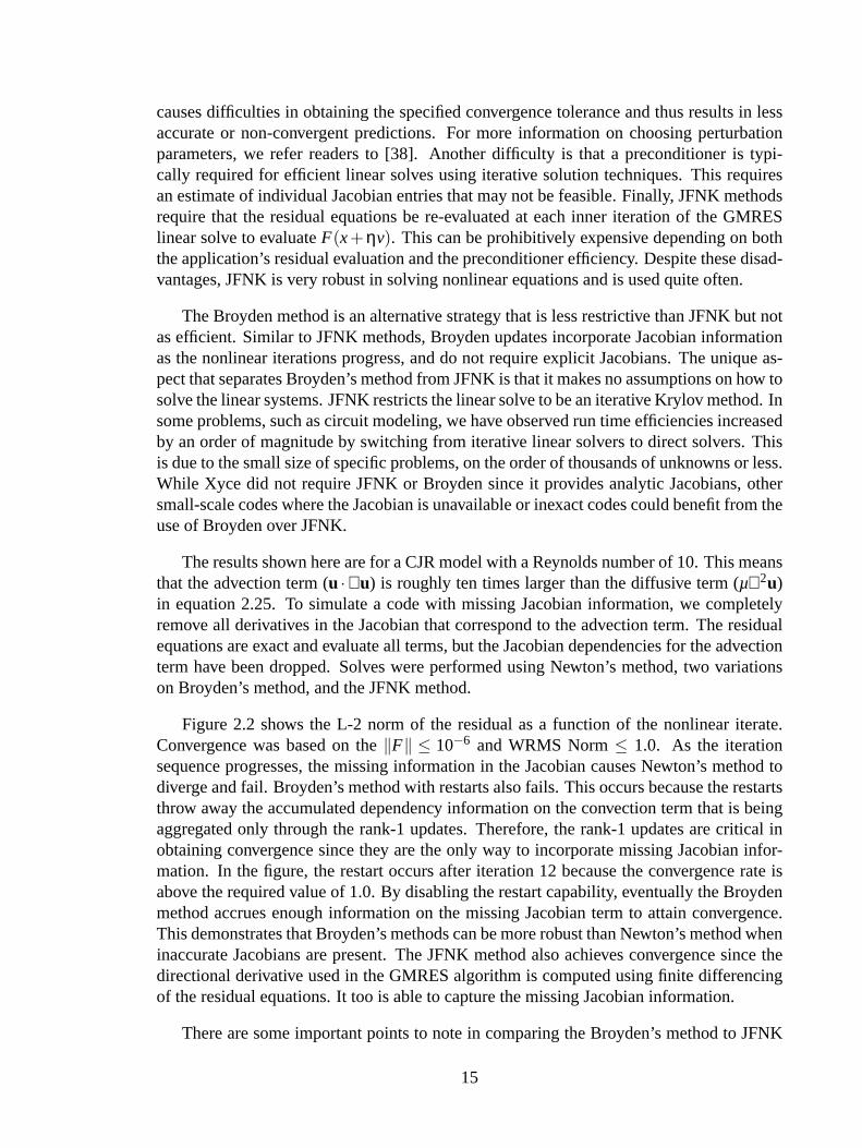
Figure 2.2 shows the L-2 norm of the residual as a function of the nonlinear iterate.Convergence was based on the‖F‖ ≤ 10−6 and WRMS Norm≤ 1.0. As the iterationsequence progresses, the missing information in the Jacobian causes Newton’s method todiverge and fail. Broyden’s method with restarts also fails. This occurs because the restartsthrow away the accumulated dependency information on the convection term that is beingaggregated only through the rank-1 updates. Therefore, the rank-1 updates are critical inobtaining convergence since they are the only way to incorporate missing Jacobian infor-mation. In the figure, the restart occurs after iteration 12 because the convergence rate isabove the required value of 1.0. By disabling the restart capability, eventually the Broydenmethod accrues enough information on the missing Jacobian term to attain convergence.This demonstrates that Broyden’s methods can be more robust than Newton’s method wheninaccurate Jacobians are present. The JFNK method also achieves convergence since thedirectional derivative used in the GMRES algorithm is computed using finite differencingof the residual equations. It too is able to capture the missing Jacobian information.
There are some important points to note in comparing the Broyden’s method to JFNK
15

Figure 2.2. Plot of the residual norm as a function of nonlineariteration number.
using Figure 2.2. First, we observe that JFNK has over-solved this problem by one nonlin-ear iteration. This is the result of the convergence criteria in the application. In particularthis is caused by the WRMS norm stopping criteria. The change in the solution vectorbetween iterates is still large, even though the tolerance for‖F‖ was met. This results inone extra nonlinear iteration in the JFNK algorithm. The second point to observe is that theconvergence for JFNK is superlinear while Broyden’s method exhibits linear convergence.Broyden’s method takes about three times as many nonlinear iterations to converge as doesJFNK.
Figure 2.2 does not give enough information to determine which method, Broydenor JFNK, should be used for a given application. The reason is that the total numberof nonlinear iterations does not directly correlate to the efficiency of the code since thelinear solves are much more expensive in JFNK. In table 2.1 we show the performancecharacteristics for the two methods that converged, Broyden without restarts and JFNK. NSis the total number of nonlinear iterations, F is number of residual (function) evaluations, Jis the number of Jacobian evaluations, LSI is the number of linear solve iterations (i.e., thenumber of GMRES iterations), F Time is the total time taken to evaluate the residuals, JTime is the total time to evaluate the Jacobians, LS Time is the total time spent in the linearsolve routines, and Total Time is the total run time. All times are reported in seconds. The
16
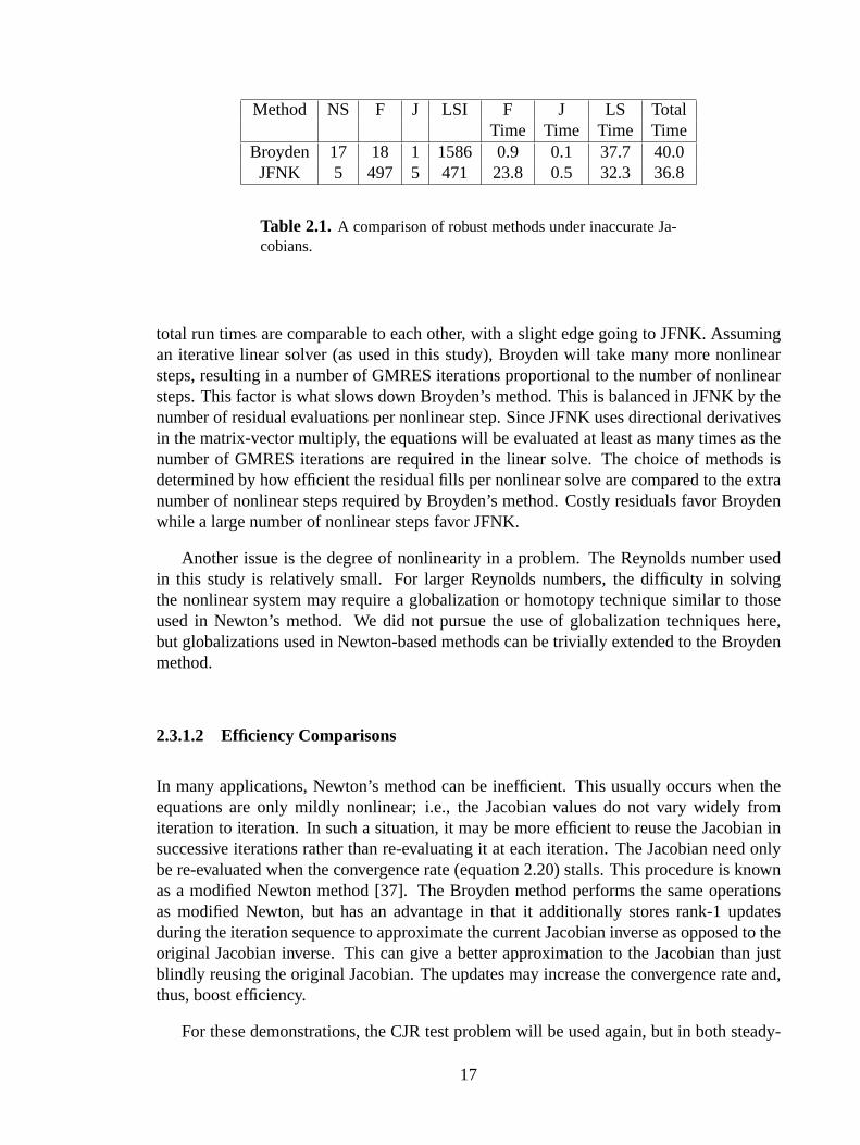
Method NS F J LSI F J LS TotalTime Time Time Time
Broyden 17 18 1 1586 0.9 0.1 37.7 40.0JFNK 5 497 5 471 23.8 0.5 32.3 36.8
Table 2.1.A comparison of robust methods under inaccurate Ja-cobians.
total run times are comparable to each other, with a slight edge going to JFNK. Assumingan iterative linear solver (as used in this study), Broyden will take many more nonlinearsteps, resulting in a number of GMRES iterations proportional to the number of nonlinearsteps. This factor is what slows down Broyden’s method. This is balanced in JFNK by thenumber of residual evaluations per nonlinear step. Since JFNK uses directional derivativesin the matrix-vector multiply, the equations will be evaluated at least as many times as thenumber of GMRES iterations are required in the linear solve. The choice of methods isdetermined by how efficient the residual fills per nonlinear solve are compared to the extranumber of nonlinear steps required by Broyden’s method. Costly residuals favor Broydenwhile a large number of nonlinear steps favor JFNK.
Another issue is the degree of nonlinearity in a problem. The Reynolds number usedin this study is relatively small. For larger Reynolds numbers, the difficulty in solvingthe nonlinear system may require a globalization or homotopy technique similar to thoseused in Newton’s method. We did not pursue the use of globalization techniques here,but globalizations used in Newton-based methods can be trivially extended to the Broydenmethod.
2.3.1.2 Efficiency Comparisons
In many applications, Newton’s method can be inefficient. This usually occurs when theequations are only mildly nonlinear; i.e., the Jacobian values do not vary widely fromiteration to iteration. In such a situation, it may be more efficient to reuse the Jacobian insuccessive iterations rather than re-evaluating it at each iteration. The Jacobian need onlybe re-evaluated when the convergence rate (equation 2.20) stalls. This procedure is knownas a modified Newton method [37]. The Broyden method performs the same operationsas modified Newton, but has an advantage in that it additionally stores rank-1 updatesduring the iteration sequence to approximate the current Jacobian inverse as opposed to theoriginal Jacobian inverse. This can give a better approximation to the Jacobian than justblindly reusing the original Jacobian. The updates may increase the convergence rate and,thus, boost efficiency.
For these demonstrations, the CJR test problem will be used again, but in both steady-
17

Run Method Max S/F NS F J F J Prec LS TotalRate Time Time Time Time Time
1 Newton NA S 5 6 5 0.3 0.6 2.3 11.7 16.02 Mod. Newton 0.1 S 7 8 3 0.4 0.3 1.4 15.8 19.13 Broyden 0.1 S 7 8 3 0.4 0.3 1.4 15.9 19.64 Mod. Newton 1.0 S 14 15 2 0.7 0.2 0.9 31.7 34.95 Broyden 1.0 S 21 22 4 1.1 0.4 1.8 53.1 57.9
Table 2.2.Steady-state performance characteristics.
state and transient modes. The runs will use the full analytic Jacobian including all inter-equation dependencies. We will compare Newton’s method, Broyden’s method and themodified Newton method. For the Broyden and modified Newton runs, we performed twosets of simulations using different values of the convergence rate,αk (section 2.2). Thevalues used are 0.1 and 1.0. The smaller the value, the more often restarts occur, makingthe methods act more like the Newton method in terms of performance.
Table 2.2 shows the steady-state problem results at a Reynolds number of 10. Max Rateis the largest value of convergence rate allowed before a restart is performed. S/F standsfor successful convergence or failure of the simulation. NS, F, and J are the number ofnonlinear steps, the number of residual (function) evaluations, and the number of Jacobianevaluations, respectively. F Time, J Time, Prec Time, LS Time, and Total Time are thetime taken for residual evaluations, time taken for all Jacobian evaluations, time taken forall preconditioner factorizations, time taken for the linear solve (excluding preconditionerfactorization time), and the total simulation time, respectively. All times are reported inseconds.
We observed that Newton’s method performs the most efficiently while Broyden’smethod with a convergence rate restart value of 1.0 performed the least. This can be at-tributed to the application code’s efficient implementation of the Jacobian evaluation andfast preconditioners. Broyden’s method is expected to out-perform Newton’s method whenthe Jacobian evaluations are expensive. In the case of MPSalsa, the Jacobian evaluationswere extremely efficient and did not factor into the overall run time. In our experience withMPSalsa, we found that the residual and Jacobian fill times were less than 10% of the totalrun time. A similar situation exists for the preconditioner. In Table 2.2 the time spent inthe preconditioner is also negligible to the overall time. Our conclusion is that in terms ofefficiency, MPSalsa should be using Newton’s method for steady-state solves.
Transient simulations were also performed for the CJR problem. Transient problemsare different from steady-state problems in that the nonlinear solves have a good initialguess from the last time step and are much more robust. This allows for good efficiencygains through reuse of the Jacobian and preconditioner because the initial values should notchange appreciably due to the good initial guess (unless very large time steps are used).
18
Run Method Max S/F NS F J F J Prec LS TotalRate Time Time Time Time Time
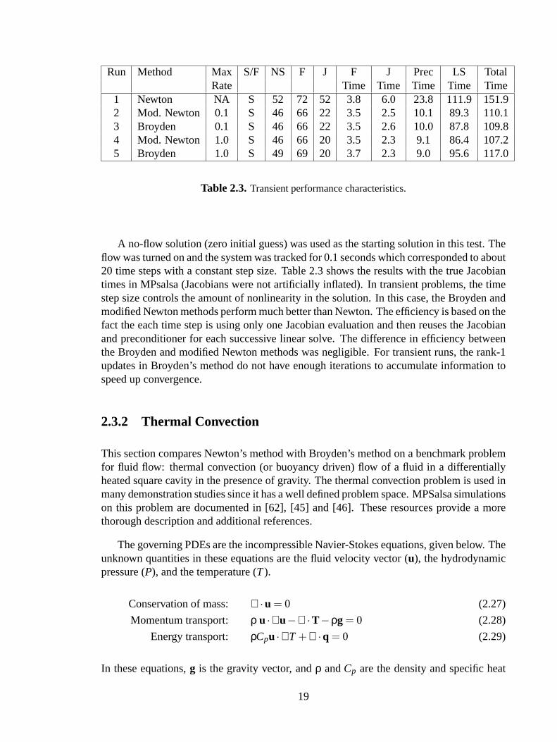
1 Newton NA S 52 72 52 3.8 6.0 23.8 111.9 151.92 Mod. Newton 0.1 S 46 66 22 3.5 2.5 10.1 89.3 110.13 Broyden 0.1 S 46 66 22 3.5 2.6 10.0 87.8 109.84 Mod. Newton 1.0 S 46 66 20 3.5 2.3 9.1 86.4 107.25 Broyden 1.0 S 49 69 20 3.7 2.3 9.0 95.6 117.0
Table 2.3.Transient performance characteristics.
A no-flow solution (zero initial guess) was used as the starting solution in this test. Theflow was turned on and the system was tracked for 0.1 seconds which corresponded to about20 time steps with a constant step size. Table 2.3 shows the results with the true Jacobiantimes in MPsalsa (Jacobians were not artificially inflated). In transient problems, the timestep size controls the amount of nonlinearity in the solution. In this case, the Broyden andmodified Newton methods perform much better than Newton. The efficiency is based on thefact the each time step is using only one Jacobian evaluation and then reuses the Jacobianand preconditioner for each successive linear solve. The difference in efficiency betweenthe Broyden and modified Newton methods was negligible. For transient runs, the rank-1updates in Broyden’s method do not have enough iterations to accumulate information tospeed up convergence.
2.3.2 Thermal Convection
This section compares Newton’s method with Broyden’s method on a benchmark problemfor fluid flow: thermal convection (or buoyancy driven) flow of a fluid in a differentiallyheated square cavity in the presence of gravity. The thermal convection problem is used inmany demonstration studies since it has a well defined problem space. MPSalsa simulationson this problem are documented in [62], [45] and [46]. These resources provide a morethorough description and additional references.
The governing PDEs are the incompressible Navier-Stokes equations, given below. Theunknown quantities in these equations are the fluid velocity vector (u), the hydrodynamicpressure (P), and the temperature (T).
Conservation of mass: ∇ ·u = 0 (2.27)
Momentum transport: ρ u ·∇u−∇ ·T−ρg = 0 (2.28)
Energy transport: ρCpu ·∇T +∇ ·q = 0 (2.29)
In these equations,g is the gravity vector, andρ andCp are the density and specific heat
19
Run Method Max S/F NS F J F J LS Prec TotalRate Time Time Time Time Time
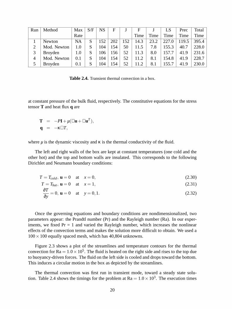
1 Newton NA S 152 202 152 14.3 23.2 227.0 119.5 395.42 Mod. Newton 1.0 S 104 154 50 11.5 7.8 155.3 40.7 228.03 Broyden 1.0 S 106 156 52 11.3 8.0 157.7 41.9 231.64 Mod. Newton 0.1 S 104 154 52 11.2 8.1 154.8 41.9 228.75 Broyden 0.1 S 104 154 52 11.2 8.1 155.7 41.9 230.0
Table 2.4.Transient thermal convection in a box.
at constant pressure of the bulk fluid, respectively. The constitutive equations for the stresstensorT and heat fluxq are
T = −PI +µ(∇u+∇uT),q = −κ∇T,
whereµ is the dynamic viscosity andκ is the thermal conductivity of the fluid.
The left and right walls of the box are kept at constant temperatures (one cold and theother hot) and the top and bottom walls are insulated. This corresponds to the followingDirichlet and Neumann boundary conditions:
T = Tcold, u = 0 at x = 0, (2.30)
T = Thot, u = 0 at x = 1, (2.31)∂T∂y
= 0, u = 0 at y = 0,1. (2.32)
Once the governing equations and boundary conditions are nondimensionalized, twoparameters appear: the Prandtl number (Pr) and the Rayleigh number (Ra). In our exper-iments, we fixed Pr = 1 and varied the Rayleigh number, which increases the nonlineareffects of the convection terms and makes the solution more difficult to obtain. We used a100×100 equally spaced mesh, which has 40,804 unknowns.
Figure 2.3 shows a plot of the streamlines and temperature contours for the thermalconvection for Ra= 1.0×10⁵. The fluid is heated on the right side and rises to the top dueto buoyancy-driven forces. The fluid on the left side is cooled and drops toward the bottom.This induces a circular motion in the box as depicted by the streamlines.
The thermal convection was first run in transient mode, toward a steady state solu-tion. Table 2.4 shows the timings for the problem at Ra= 1.0×10³. The execution times
20
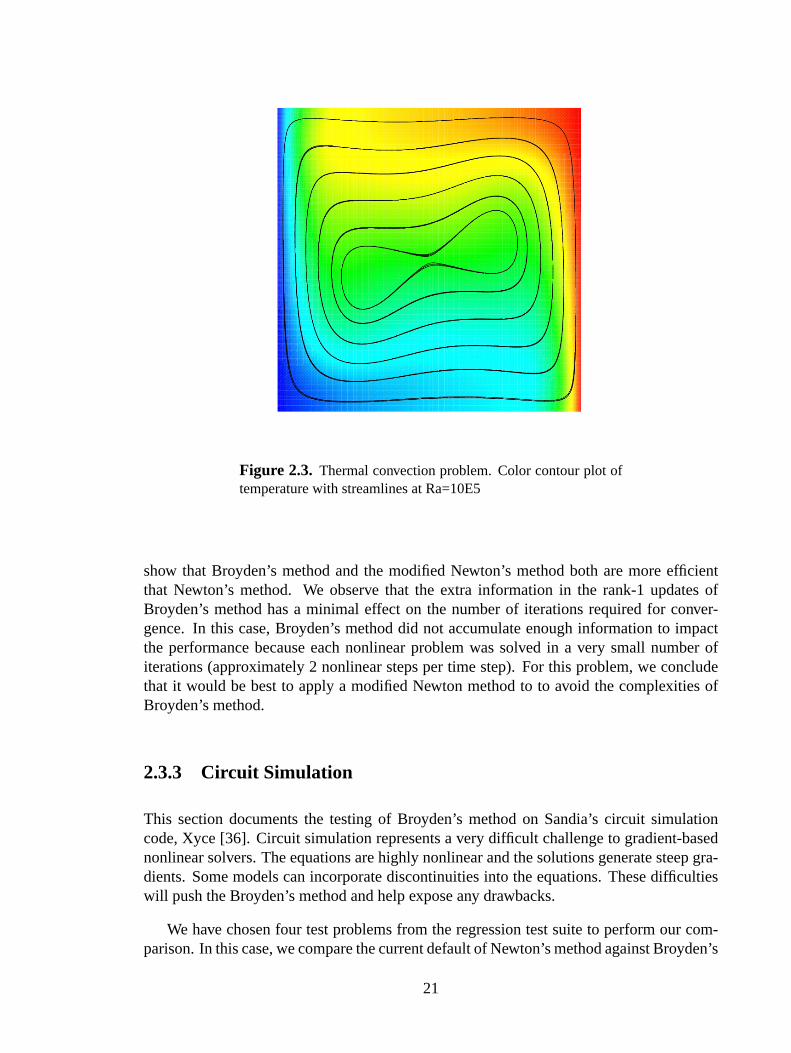
Figure 2.3. Thermal convection problem. Color contour plot oftemperature with streamlines at Ra=10E5
show that Broyden’s method and the modified Newton’s method both are more efficientthat Newton’s method. We observe that the extra information in the rank-1 updates ofBroyden’s method has a minimal effect on the number of iterations required for conver-gence. In this case, Broyden’s method did not accumulate enough information to impactthe performance because each nonlinear problem was solved in a very small number ofiterations (approximately 2 nonlinear steps per time step). For this problem, we concludethat it would be best to apply a modified Newton method to to avoid the complexities ofBroyden’s method.
2.3.3 Circuit Simulation
This section documents the testing of Broyden’s method on Sandia’s circuit simulationcode, Xyce [36]. Circuit simulation represents a very difficult challenge to gradient-basednonlinear solvers. The equations are highly nonlinear and the solutions generate steep gra-dients. Some models can incorporate discontinuities into the equations. These difficultieswill push the Broyden’s method and help expose any drawbacks.
We have chosen four test problems from the regression test suite to perform our com-parison. In this case, we compare the current default of Newton’s method against Broyden’s
21
Test Circuit Method S/F NS F J TotalTime
Comparator Newton S 3439 5120 3439 0.80Broyden S 3528 5206 1729 0.79
Dual Channel Newton S 9047 11495 9047 8.34Broyden F 12572 14311 4985 16.7
Single Channel Newton F 30702 57731 31942 135.0Broyden S 100589 264003 53563 417.0
ssunone Newton S 385165 556754 385165 181.4Broyden F 227328 327575 102702 101.7
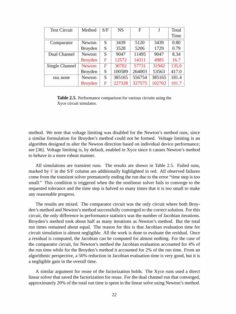
Table 2.5.Performance comparison for various circuits using theXyce circuit simulator.
method. We note that voltage limiting was disabled for the Newton’s method runs, sincea similar formulation for Broyden’s method could not be formed. Voltage limiting is analgorithm designed to alter the Newton direction based on individual device performance;see [36]. Voltage limiting is, by default, enabled in Xyce since it causes Newton’s methodto behave in a more robust manner.
All simulations are transient runs. The results are shown in Table 2.5. Failed runs,marked byF in the S/F column are additionally highlighted in red. All observed failurescome from the transient solver prematurely ending the run due to the error “time step is toosmall.” This condition is triggered when the the nonlinear solver fails to converge to therequested tolerance and the time step is halved so many times that it is too small to makeany reasonable progress.
The results are mixed. The comparator circuit was the only circuit where both Broy-den’s method and Newton’s method successfully converged to the correct solution. For thiscircuit, the only difference in performance statistics was the number of Jacobian iterations.Broyden’s method took about half as many iterations as Newton’s method. But the totalrun times remained about equal. The reason for this is that Jacobian evaluation time forcircuit simulation is almost negligible. All the work is done to evaluate the residual. Oncea residual is computed, the Jacobian can be computed for almost nothing. For the case ofthe comparator circuit, for Newton’s method the Jacobian evaluation accounted for 4% ofthe run time while for the Broyden’s method it accounted for 2% of the run time. From analgorithmic perspective, a 50% reduction in Jacobian evaluation time is very good, but it isa negligible gain in the overall time.
A similar argument for reuse of the factorization holds. The Xyce runs used a directlinear solver that saved the factorization for reuse. For the dual channel run that converged,approximately 20% of the total run time is spent in the linear solve using Newton’s method.
22

If Broyden’s method had converged, it could only improve on a fraction of that 20%. Theleads us to conclude that for circuit simulation, with respect to efficiency, the main advan-tages in using Broyden’s method is lost. The ability to reuse the Jacobian and factorizationeach lead to little gain, because most of the work occurs in the residual evaluation.
The other problems either converged with Newton or converged with Broyden but notboth. This shows that in circuits, the path an algorithm traverses is important in achievingconvergence. If circuit simulators have convergence problems with Newton’s method, oneoption would be to try using Broyden’s method. In our experience with circuit simulation,voltage limiting has been the most successful option.
The Xyce circuit simulator constructs analytic Jacobians and therefore does not needto use JFNK or Broyden’s method. Therefore, we do not recommend the general use ofBroyden’s method in Xyce. The only situation it may be of some assistance is if Newton’smethod fails.
2.4 Discussion
We implemented a modified version of Kelley’s [37] limited-memory Broyden algorithmand tested it on large-scale problems on parallel machines. We made certain implementa-tion choices to make the method robust. Broyden’s method is similar to Newton’s methodbut does not require a Jacobian be explicitly evaluated. Instead, a Jacobian estimate is con-structed using a series of rank-1 updates to some initial guess. An added expense of storingone extra vector per nonlinear iteration is incurred.
Testing has demonstrated that Broyden’s method can be used as a successful alternativeto the JFNK method for solving systems where the Jacobian either cannot be computedexplicitly or the estimation of the Jacobian is poor. Broyden’s method may be more efficientthan JFNK in cases where a large fraction of the run time is associated with the residualevaluations. In addition, the Broyden method does not require an iterative linear solver, asdoes JFNK, making it a more generally applicable algorithm.
An efficiency study has demonstrated that problems exist where Broyden’s method canbe more efficient than Newton’s method. The efficiency comes from the fact that Broydencan reuse the Jacobian and the factorization/preconditioner for the linear solves. Thesemethods are most useful when the problems are mildly nonlinear. Such cases arise mostoften from transient solves since there is a good initial guess and the time step size cancontrol the degree of nonlinearity.
If the Broyden updates are not stored, Broyden’s algorithm reduces to a modified New-ton method. Comparing against modified Newton, we could isolate the effects of the rank-1updates. In terms of efficiency, the updates do not play a critical role. These cases typicallyrequire very few nonlinear iterations (less than 10) and the updates fail to generate a goodapproximation to the Jacobian in such a small space. We do note, however, that in terms of
23

robustness, the rank-1 updates can be critical if the Jacobian is inaccurate. As demonstratedin section 2.3.1.1, the updates aggregate information on the missing/inexact Jacobian termsto attain convergence at the cost of taking a larger number of Newton steps.
The Broyden algorithm has been implemented in the NOX Nonlinear Solver Library[41] and is available for download under the GNU LPGL license.
24

Chapter 3
Tensor Methods
In this chapter, we present our work with tensor methods [57] for solving large-scale sys-tems of nonlinear equations. We discuss methods that were implemented in the nonlin-ear software package NOX [41] and our modifications to the tensor-Krylov method ofBouaricha [9], which considers a special case in a new way and improves its numericalperformance. This research is aimed at studying the efficiency and robustness of tensormethods for problems at Sandia. In addition, we hope to bring tensor methods more intothe mainstream by offering an implementation that can use any linear solver.
3.1 Introduction
Standard methods for solving the nonlinear equations problem (1.1), such as Newton’smethod, base each iteration upon a local, linear modelM(xk + d) of the functionF(x)around the current iteratexk ∈ Rn. These methods work well for problems with well-conditioned Jacobians at the solution (they have a quadratic convergence rate), but they facedifficulties when the Jacobian is singular or nearly singular at the solution. Many authorshave analyzed the behavior of Newton’s method on singular problems and have proposedacceleration techniques as remedies (see, e.g., Decker, Keller, and Kelley [14]; Decker andKelley [15, 16, 17]; Griewank [29]; Griewank and Osborne [31]; Kelley and Suresh [39];and Reddien [47]). Their collective analysis shows that Newton’s method without accel-eration is locallyq-linearly convergent with the ratio of the norm of consecutive residualsconverging to1
2. Acceleration techniques address this deficiency to some extent, but theyrequirea priori knowledge that the problem is singular, which is not practical for generalproblem solving.
Tensor methods for nonlinear equations [57] do not requirea priori knowledge ofwhether the Jacobian at the solution is singular or ill-conditioned (henceforth we just referto the problem as being “singular” or “ill-conditioned”). They bypass this precondition by
25
always including second-order information at each iteration in the local model:
MT(xk +d) = F(xk)+J(xk)d+ 12Tkdd,
whereTk ∈ Rn×n×n is a low-rank approximation toF ′′(xk), usually formed by a secant ap-proximation. As a result, tensor methods have local superlinear convergence for a largeclass of singular problems under mild conditions [23]. Specifically, [23] shows that onproblems where the rank of the Jacobian at the root isn− 1, “practical” tensor methods(i.e., those using secant approximations for the tensor termTk) have three-step superlin-ear convergence behavior withq-order 3
2. In practice, one-step superlinear convergencefrequently is observed on these problems. (Recall that Newton’s method without any ac-celeration techniques on such problems exhibits onlyq-linear convergence.) In addition,the analysis in [23] shows that tensor methods have at least quadratic convergence on non-singular problems.
The additional termTk present in tensor methods provides second-order informationin recent step directions, which aids in cases where the Jacobian is (nearly) singular atthe solution. As the iterates approach the solution, the Jacobian lacks information in thenull space direction, but the second-order term supplies useful information for a betterquality step. Computational evidence in [57] on small problems shows that tensor methodsprovide 21–23% average improvement (in terms of function evaluations and/or nonlineariterations) over standard methods on nonsingular problems and 40–43% improvement onproblems with rank(J(x∗)) = n−1. Thus, while tensor methods are not widely adopted,they generally outperform standard methods, particularly on ill-conditioned and singularproblems.
Tensor methods that solve the local model with a direct factorization of the Jacobianmatrix (like standard Newton’s method) cannot efficiently solve large-scale problems dueto large storage considerations and the expensive direct solution of the tensor model. To thisend, several versions of inexact tensor methods have been developed for solving large prob-lems. Bouaricha [9] describes an implementation that uses a Krylov-based linear solver andconstructs an inexact tensor step from the approximate solutions of two linear systems (withthe same Jacobian matrix). Feng and Pulliam [24] have developed a “tensor-GMRES”method, which first finds the Newton-GMRES step and then solves for an approximatetensor step. More recently, Bader has developed a class of methods called tensor-Krylovmethods [2, 3] that calculates a tensor step from a specially chosen Krylov subspace. All ofthese algorithms are an amalgamation of various techniques, including tensor methods fornonlinear equations [57], Krylov subspace techniques [12], and an inexact solver frame-work [18], that make them well-suited for large-scale problems.
These large-scale tensor methods have advantages and disadvantages, especially whenconsidering the development cost of implementing them in a production code, such asNOX. For example, while the tensor-Krylov methods generally have superior performanceand better theoretical properties than the other methods, they are more complicated to im-plement due to a specialized local solver. On the other hand, Bouaricha’s tensor method issimple to implement because it can use any linear solver, but it generally requires twice thetotal number of linear iterations as the others and gives up some theoretical guarantees.
26
It is with these tradeoffs in mind that we focused our research to develop a new tensormethod resulting in a modification to Bouaricha’s method that has good theoretical proper-ties. The modified Bouaricha tensor method is implemented in the NOX Nonlinear SolverLibrary [41], which is available for download under the GNU LPGL license.
3.2 Background on Tensor Methods
Some background on tensor methods will be helpful and is described here. In the first sub-section, we review the tensor methods as they were introduced in [57] and also discuss analternative algorithm introduced in [9]. Since these standard approaches use direct factor-izations of the Jacobian matrix, we refer to these methods as direct tensor methods. Dueto the storage and linear algebra costs, these methods are only practical for solving small,dense problems. The last subsection discusses simple global strategies used by tensor meth-ods, which require a modification to the standard global strategies because the tensor stepis not guaranteed to be a descent direction.
3.2.1 Tensor Methods
Tensor methods were first proposed by Schnabel and Frank [57] and since have been stud-ied by many others [2, 3, 9, 23, 24]. In deriving tensor methods for nonlinear equations, weconsider the Taylor series expansion ofF(x) aroundxk:
F(xk +d) = F(xk)+F ′(xk)d+ 12F ′′(xk)dd+O(d3). (3.1)
Whereas Newton’s method solves the first-order Taylor series approximation at each it-eration, tensor methods include a special, restricted form of the quadratic term from theTaylor’s expansion. While it would be impractical to actually form and storeF ′′(xk) (i.e.,12n3 second partial derivatives ofF(x)), further complications for solving a system ofnquadratic equations inn unknowns would render this direct approach prohibitive. Thus,practical tensor methods store a secant approximation toF ′′(xk)dd based on informationfrom previous iterations, similar to the concept of secant approximations for approximat-ing the Jacobian (as in Broyden’s method). At each iteration, a low-rank approximationto F ′′(xk) is formed, which requires considerably less storage and allows the model to besolved efficiently. Augmenting the linear model with this term yields what we call the localtensor model:
MT(xk +d) = F(xk)+J(xk)d+ 12Tkdd, (3.2)
whereTk ∈ Rn×n×n is a low-rank approximation toF ′′(xk). The termTk is selected so thatthe model interpolatesp≤
√n previous function values in the recent history of iterates,
which makesTk a rank-p tensor. Computational evidence in [57] suggests thatp > 1 addslittle to the computational performance of a direct tensor method, so we focus on the caseof p = 1, which uses only one secant update and creates a rank-1 tensor. There may be
27
scenarios in which a higher-rank approximation may be useful, such as dealing with aJacobian having a rank less thann−1.
In the case ofp = 1, the tensor model aboutxk reduces to
MT(xk +d) = Fk +Jkd+ 12ak(sT
k d)2, (3.3)
where
ak ∈ Rn =2(Fk−1−Fk−Jksk)
(sTk sk)2
, (3.4)
sk ∈ Rn = xk−1−xk. (3.5)
After forming the model, we use it to determine the step to the next trial point. Because(3.3) may not have a root, we solve the minimization subproblem
mind∈Rn‖MT(xk +d)‖2 , (3.6)
and a root or minimizer of the model is the tensor step. Due to the special form of (3.3),the solution of (3.6) in the nonsingular case reduces to minimizing a quadratic equationfollowed by solving a system ofn−1 linear equations in as many unknowns.
This minimization problem may be solved in a variety of ways. Schnabel and Frank[57], for example, show how to find the solution for arbitraryp using orthogonal trans-formations, and this method is described first. An alternative approach by Bouaricha [9],based on a reduced system whenp = 1, is described later. Background in both approachesis useful for introducing the large-scale tensor methods.
3.2.1.1 Method of Orthogonal Transformations
The first approach for solving (3.6) uses two orthogonal transformations to reduce the prob-lem to two subproblems that are more easily solved. We refer to [57] for more details, butbriefly the approach is as follows. The first transformation finds an orthogonalQ1 ∈ Rn×n
such thatsk/‖sk‖ is the last column and permits a change in variables
d = Q1d.
The second transformation finds an orthogonalQ2 ∈ Rn×n such thatQ2JkQ1 is upper tri-angular. Applying these two transformations to (3.3) and setting the system equal to zero,yields the following triangular system ofn equations inn unknowns
Q2Fk +Q2JkQ1d+ 12Q2ak‖sk‖2 d2
n = 0, (3.7)
wheredn ∈ R is the unknown appearing in the quadratic equation.
28
Partitioning (3.7) into two smaller problems, the solution to (3.6) continues by firstsolving for dn by minimizing the quadratic equation appearing in the last row of (3.7) andchoosing the smaller magnitude minimizer if there are two. Using the value ofdn in (3.7), atriangular linear system of size(n−1)× (n−1) is revealed. Finally, the complete solutionto (3.6) is found by solving this resultant system for the remaining components ofd andthen reversing the variable space transformation from the first step,d = Q1d.
3.2.1.2 Reduction Method
The second approach due to Bouaricha [9] for solving the tensor model (3.6) involvessolving a reduced system of quadratic equations after first solving two linear systems withthe same Jacobian matrix. The method may handle an arbitrary size ofp, but we willrestrict ourselves to the casep = 1. We will call this approach the “reduction method”because it solves two linear systems and then reduces the system of quadratic equations toa single quadratic equation.
In this approach, the tensor step is found by multiplying (3.3) bysTk J−1
k and finding theroot or minimizer of the resulting equation,
sTk J−1
k Fk +sTk d+ 1
2sTk J−1
k ak(sTk d)2 = 0. (3.8)
Defining the quantitysTk d asβ, a quadratic equation inβ—call it q(β)—is revealed,
β ≡ sTk d
q(β) ≡ sTk J−1Fk +β+ 1
2sTk J−1
k akβ2. (3.9)
Since (3.9) may or may not have a root, solving the single-variable minimization problem
minβ∈R|q(β)| (3.10)
provides the valueβ∗. If q(β) has two real roots, then the root of smaller magnitude istaken. To solve the original problem and find the tensor step, we calculate the value ofq(β∗) and substitute this value andβ∗ into the explicit step
dT =−J−1k
[Fk + 1
2akβ2∗−
J−Tk skq(β∗)
sTk (JT
k Jk)−1sk
]. (3.11)
We omit the proof that this step solves the tensor model (see [9] for details), but one canverify that the step (3.11) is a root or minimizer of (3.3) by substituting it into the model,simplifying, and recalling the definitionβ∗ = sT
k dT and thatq(β∗) has minimum norm.Quite oftenq(β∗) = 0, which avoids computing the last term. This term requires a non-trivial amount of extra arithmetic to form, so the large-scale implementation in [9] actuallyneglects this term without apparent detriment.
29
The operation count of this process whenp = 1 is the cost of a matrix factorization ofthe JacobianJk, two back substitutions using this factorization, plus the cost of minimizing(3.10), which for this case ofp = 1 a closed form solution exists. Thus, the total costbeyond a standard method is aboutn2 multiplications due to the extra linear solve (ignoringthe extra term ifq(β∗) is nonzero).
If during an iteration the Jacobian is singular, then a modified approach may be takenwith thisq(β) formulation. It involves changing the Jacobian to be nonsingular, modifyingthe function value, and redefiningβ, all in a way that still results in solving the originalmodel. The modified tensor model becomes
MT(xk +d) = Fk + Jkd+ 12akβ,
whereJk equalsJk plus a low-rank matrix. This technique is not new, but it has not beenpublished in much detail. We will discuss it in more detail in section 4.1.1.
3.2.2 Global Strategies
To achieve global convergence, most tensor method implementations use a line search strat-egy for its simple implementation and reasonable robustness. To complete this section’sbackground review of tensor methods, we provide brief descriptions of a common tensormethod line search strategy and the more advanced curvilinear line search.
First, we present the line search strategy introduced in [57], which chooses between thetensor step and the Newton step for the search direction for backtracking. This strategyalways attempts the full tensor step first to preserve convergence properties of the tensormethod. However, because the tensor step is not guaranteed to be a descent direction on themerit function f (x) = ‖F(x)‖, a “backup” descent direction is needed if the first trial pointis not acceptable and the tensor step is not a descent direction. Fortunately, the Newtondirection is guaranteed to be a descent direction on the merit function, which would beused in place of the tensor step in such cases. An important aspect of tensor methods forsmall, dense systems is that the Newton step can be computed readily with an extra linearsolve by ignoring the tensor term (or the Newton step is already computed with the methodof Bouaricha).
To be precise, the line search algorithm for step selection from [57], which we call the“standard tensor line search,” is presented here:
Algorithm 2.1: STANDARD TENSORL INE SEARCH
If (no root or minimizer of the tensor model could be computed)Or ((minimizer of tensor model that is not a root was found)And (‖MT(xk +dT)‖2 > 1
2 ‖F(xk)‖2)),
30
Thenxk+1← xk +λdN,λ ∈ (0,1] selected by line search;
Elsexk+1← xk +dT .
If xk+1 is not acceptable, then
If dT is a sufficient descent direction.
Thenxk+1← xk +λdT ,λ ∈ (0,1] selected by line search;
Elsexk+1← xk +λdN,λ ∈ (0,1] selected by line search.
As can be seen, different conditions necessitate line searches with either the tensor stepor the Newton step (dT or dN).
The second global strategy we present is the curvilinear line search [4]. The curvilin-ear line search involves the solution of the modified tensor modelλF + Jd+ 1
2a(sTd)2,whereλ ∈ (0,1] is the line search parameter. As the value ofλ changes according to someprescribed procedure (e.g., quadratic backtracking or interval halving), the solution to themodified tensor model is the curvilinear stepdT(λ). The curvilinear step has some nice the-oretical properties, including guaranteed descent asλ→ 0 and monotonicity on the meritfunction. Unlike the standard tensor line search, the curvilinear line search obviates theneed for special cases because it sweeps out a path spanned by the Newton direction andthe tensor step. In that regard, the curvilinear line search is similar to a trust region method(cf. the optimal hook step [19]), which spans the steepest descent direction and Newtonstep.
3.3 Review of Large-scale Methods
In the previous section, we reviewed direct tensor methods. We now shift our focus tosolving large, sparse problems, which requires a different approach to be computationallyefficient and have low storage requirements. Three classes of large-scale tensor methodsalready exist and are predicated upon Krylov subspace methods.
We begin the discussion by reviewing inexact Newton methods [18] and, in particular,Newton-Krylov methods [12], where linear Krylov subspace methods solve the local modelto some relative tolerance. Then we review the tensor-Krylov method of Bouaricha [9],tensor-GMRES of Feng and Pulliam [24], and the tensor-Krylov methods of Bader [2, 3].
3.3.1 Newton-Krylov Methods
Large, sparse nonlinear systems often are solved successfully using a class of “inexact”Newton methods:
xk+1 = xk +dk, where J(xk)dk =−F(xk)+ rk, ‖rk‖ ≤ ηk‖F(xk)‖ . (3.12)
31

The local model is solved only approximately at each step using an iterative linear solver.
A common approach for approximately solving the local Newton model in (3.12) usesKrylov-based methods [12]. A linear Krylov subspace method is a projection method thatseeks an approximate solutionxm to the linear systemAx= b from anm-dimensional affinesubspacex0 +Km. Here,Km is the Krylov subspace
Km(A, r0) = spanr0,Ar0,A2r0, . . . ,A
m−1r0,
wherer0 = b−Ax0 is the residual at an initial guessx0. A popular Krylov subspace methodis the Generalized Minimum Residual method (GMRES) [52], which computes a solutionxm∈ x0+Km such that the residual norm over all vectors inx0+Km is minimized. That is,at themth step, GMRES findsxm such that‖b−Axm‖2 is minimized for allxm∈ x0 +Km.One drawback of GMRES is the storage requirement of an orthogonal basis, which couldbe larger than a sparse Jacobian matrix unlessm is kept small, leading to the class ofrestarted GMRES methods [52]. Other Krylov methods, such as BiCGSTAB and TFQMR(see, e.g., [51]), do not have these additional storage requirements but may not be as robust.A Newton-based method that uses GMRES as its local solver is called Newton-GMRES.It is a popular algorithm for solving large-scale problems and will be used as the standardNewton-based algorithm in our numerical experiments.
3.3.2 Bouaricha’s Method
As presented in section 3.2.1, the tensor step is calculated in one of two ways: (1) usingorthogonal transformations for small, dense problems, or (2) using the reduction methodfor both sparse and dense systems (but with more difficulty if the Jacobian is singular or ifthe model does not have a root).
With the reduction method, one needs the valuessTJ−1F andsTJ−1a in equation (3.9)to find the value ofβ∗. The advantage of the reduction method is that any linear solver maybe used to solve these linear systems, which makes the method noninvasive. For instance,efficient Krylov methods may be used for solving the linear systemsJ−1F andJ−1a, po-sitioning them for use on large-scale problems. Indeed, this is the approach adopted byBouaricha in [9] for a large-scale tensor method, which he calls a tensor-Krylov method.We believe this is an unfortunate name because the method is not restricted to using Krylov-based linear solvers. For the sake of clarity to distinguish it from the tensor-Krylov methodsof [2, 3], we will refer to his tensor-Krylov method as “Bouaricha’s method.”
Bouaricha’s method uses principles from inexact Newton methods and expects onlyapproximate solutions to the two linear systems. Thus, when calculatingβ∗ from (3.10),the value ofβ∗ will be inexact, but hopefully a good enough estimate.
A key point of Bouaricha’s algorithm, however, differentiates it from a straightforwardimplementation that uses just the concepts above. For this discussion let the previous non-linear iterate be denoted with the subscriptk−1. So instead of approximately solving the
32
systemJ−1k ak, his method solves a different linear problem,J−1
k Fk−1, and then reachesJ−1
k ak via the linear combination: 2(J−1k Fk−1− J−1
k Fk− sk)/(sTk sk)2. The beauty of this
approach is due to a clever initial guess for the second system,J−1k Fk−1. Because the Jaco-
bian typically changes very little from iteration to iteration near the solution, the previousNewton directionJ−1
k−1Fk−1 will be close toJ−1k Fk−1 if the Jacobian at the root is nonsingu-
lar. If the Jacobian is singular, then the directions are likely to be collinear but of differentmagnitudes. Thus, Bouaricha’s method uses the approximate Newton step calculated fromthe previous step as an initial guess for the systemJkw= Fk−1. The complete algorithm forsolving the local model at each nonlinear iteration is presented below.
Algorithm 3.1: BOUARICHA’ S TENSOR-KRYLOV METHOD
1. Approximately solveJkdN =−Fk for dN using a Krylov subspace method.
2. Approximately solveJky=−Fk−1 for y using a Krylov subspace method and startingfrom the initial guessy0 =−dNk−1 = J−1
k−1Fk−1.
3. Form the termw = J−1k ak by using the following relationship:
w = J−1k ak
=2
(sTk sk)2
(J−1k Fk−1−J−1
k Fk−sk)
=2
(sTk sk)2
(−y+dN−sk).
4. Form the quadratic equation
q(β) = 12sT
k J−1k akβ2 +β+sT
k J−1k Fk (3.13)
= 12sT
k wβ2 +β−sTk dN, (3.14)
and find the smallest magnitude real root or minimizer ofq(β).
5. Calculate the tensor step
dT = −J−1k Fk− 1
2J−1k akβ2
∗
= dN− 12wβ2
∗,
whereβ∗ is the solution of (3.14).
6. Select the next iteratexk+1 using a line search global strategy (as outlined in sec-tion 3.3.4.3).
33
When calculating the tensor step, Bouaricha’s method also neglects the complicatedterm in (3.11) involvingq(β∗),
(JTk Jk)−1sk
sTk (JT
k Jk)−1skq(β∗). (3.15)
The justification for this omission is that the term has a considerable computational costfor large-scale problems and that there appears to be no way to calculate it without havingall of Jk available. Also, it is proved in [9] that the step calculated without (3.15) stillretains the same convergence properties of the tensor method. As a sketch of the proof,the expression (3.15) is negligible in the neighborhood of the solution and, therefore, hasno effect on the tensor method. In the numerical experiments in [9], omitting the term hada seemingly negligible impact on the performance of the algorithm. Our modification toBouaricha’s method discussed in section 3.4 also seeks to avoid this complicated term.
Despite favorable results in [9], studies in [2] have found the method to be less impres-sive on more practical problems. The two main disadvantages of Bouaricha’s method stemfrom the fact that two linear systems must be solved for each outer iteration and that anaccurate value ofβ is not calculated. These disadvantages are discussed next.
As specified in the algorithm above, solving the two linear systems required by Bouaricha’smethod (Jkd = −Fk andJky = −Fk−1) is roughly twice the cost per nonlinear iteration ofNewton’s method. The clever initial guess for the second linear system usually does nothelp until the iterates get close to the solution, at which point typically only a few morenonlinear iterations are needed. Until then, solving the two linear systems separately dou-bles the cost per nonlinear iteration as compared with Newton’s method. Thus, for thesemethods to be competitive, the number of nonlinear iterations would need to be halved,which does not happen very frequently on practical problems.
In addition to the added cost of solving two linear systems independently, it is not clearhow precise the solutions need to be to provide an accurate value forβ in Bouaricha’smethod. This feature can be detrimental to the method by making it potentially unstable.That is, if both linear systems are solved only approximately, thenβ may be inaccurate,affecting the quality of the computed tensor step since the scalar coefficient of the vectorJ−1a is 1
2β2. Any errors inβ are magnified once the value is squared, particularly if the ap-proximate value is much larger than the true value. Thus, Bouaricha’s method can and doescompute spurious steps and performs worse than corresponding Newton-Krylov methods.
Numerical results in [2] show that these disadvantages often outweigh any benefit ofcalculating the tensor step. Indeed, testing on medium-sized problems (n < 1000) showedthat the performance of Bouaricha’s method usually trailed the performance of Newton’smethod as well as the other large-scale tensor methods. Due to the theoretical disadvantagesmentioned above and the lackluster numerical performance, this algorithm has not receivedmuch attention. In section 3.4, we will examine modifications to Bouaricha’s method thatimprove it.
34
3.3.3 Tensor-GMRES Method
Another large-scale tensor method is that of Feng and Pulliam [24]. It is also a tensor-Krylov method but employs a different strategy. It uses Krylov subspace projection tech-niques for solving the Newton equations; and, in particular, it uses GMRES to find theapproximate Newton stepdN = d0 +Vmym. Once again, the columns ofVm form an or-thonormal basis for the Krylov subspaceKm generated by the corresponding Arnoldi pro-cess, and the Hessenberg matrixHm is also generated from the Arnoldi process. Giventhese key matrices, their tensor-GMRES algorithm proceeds to solve a projected versionof the tensor model (3.3) along a subspace that spans the Newton step direction (i.e., theapproximate tensor step is in the span of the Krylov subspaceK N
m andd0, or equivalentlythe span of the matrix[Vm,d0]). Thus, their algorithm solves the least-squares problem
mind∈d0∪K N
m
∥∥Fk +Jkd+ 12Pa(sTd)2
∥∥ , (3.16)
whereP is the projection matrix
P = Y(YTY)−1YT , whereY = Jk[Vm,d0]. (3.17)
Despite the algorithm’s daunting algebra, the design is actually rather straightforward.The algorithm may be viewed as an extension of Newton-GMRES, where the inexact New-ton step is calculated via GMRES in the standard way. An approximate tensor step is calcu-lated subsequently using the Krylov subspace information generated for the Newton step.In this way, the method is also consistent with preconditioning techniques and a matrix-freeimplementation, which makes it appealing for general use. However, because it requiresthe orthogonal basisVm and Hessenberg matrixHm from the linear solver, we classify thetensor-GMRES method as an “invasive” method.
The Feng and Pulliam tensor-GMRES method for solving the local tensor model in-volves some difficult algebra, but the extra work and storage beyond GMRES is actuallyquite small. The extra work is at most 4mn+5n+2m2 + O(m) multiplications plus a sin-gle Jacobian-vector product for evaluating the rank-one tensor vectorak. The extra storageamounts to two extran-vectors forak andsk plus a few smaller working vectors of lengthm.
The analysis in [24] shows that the same superlinear convergence properties for theunprojected tensor model considered in [23] also hold for the projected tensor model (3.16).Both analyses consider ideal tensor models (i.e., whenak is formed using information fromthe singular value decomposition ofJk instead of from a secant approximation) and extendthe ideal result to practical implementations that use a secant approximation forak. Whenconsidering only ideal tensor models, the only difference between the model in [23] andthe projected model (3.16) is a projection matrixP in front of ak. In the ideal case, theprojection matrixP is the matrixWWT , such that the left singular vector corresponding tothe least singular value ofJk is in the span of the orthonormal column vectors ofW. Fengand Pulliam show that this difference does not affect the proofs of Lemmas 4.1 and 4.2 in
35

[23], so the rest of the convergence analysis follows exactly the proof of Theorem 4.4 in[23].
Feng and Pulliam extend this convergence result of an ideal, projected tensor model tothe practical, projected tensor model of (3.16) with the use of two approximations. First,the Newton direction found via GMRES,dN ∈ [Vm,d0], will be arbitrarily close tovc
N,the right singular vector corresponding to the smallest singular value ofJk. Thus, thedifference between two consecutive iterates,sk = xk−1− xk, is likely to be along the nullspace when approaching a rank-deficient solution, so a practical implementation usessk toapproximate the null space direction. Second, the ideal projection matrixWWT projectsonto the subspace containing the left singular vector corresponding to the smallest singularvalue ofJk, which is in the same direction asJkvc
N. Hence, a reasonable approximation toWWT is the projection matrix (3.17). While a rigorous proof is not provided in [24], thesetwo approximations for a practical tensor-GMRES method appear to work well in theirnumerical tests. See [23] and [24] for more theoretical details.
The Feng-Pulliam tensor-GMRES method has been tested in a variety of numericalexperiments, including comparisons in [2, 3, 4, 24]. In all, the results suggest that tensor-GMRES is a competitive algorithm that usually performs on par with other large-scaletensor methods and in some cases even better. However, there are instances when perfor-mance is hindered. These cases stem from a few theoretical deficiencies of tensor-GMRESthat are related to using a Krylov subspace generated from the solution of the Newton step.We discuss these disadvantages in more detail next.
First, the variable space restriction ond in the minimization problem (3.16) illustrates apossible disadvantage of the Feng-Pulliam method, particularly when using preconditionersor restarted GMRES. Instead of solving (3.16) in the full variable space (which wouldbe expensive), Feng and Pulliam restrict the solutiond along a subspace that spans theKrylov subspace generated from the Newton-GMRES step since the Newton step usuallyprovides good directional information. Hence, the norm of the projected tensor model isonly minimized to the extent that the Krylov subspace for the Newton-GMRES step is largeenough to capture important directional information of the second-order tensor term.
Consider, for example, using anexactpreconditioner, i.e.,M = Jk. One iteration ofGMRES solves the Newton equations exactly, and the Newton step direction isv1 fromthe orthonormal basisVm. Then, according to the Feng-Pulliam method, the approximatetensor step that solves (3.16) could only be a scalar multiple of the directionv1 (assumingthat d0 = 0). A similar example may be developed when using restarted GMRES in theFeng-Pulliam method—if GMRES converges soon after a restart, then the orthonormalbasisVm is smaller than before the restart. A smaller basis may lead to a tensor step thatsolves (3.16) with more error due to fewer degrees of freedom. Some limited testing in[2] suggests that solving (3.16) in a smaller variable space adversely affects the practicalperformance of this method when using preconditioners or restarted GMRES.
Second, the Feng-Pulliam method solves theprojectedtensor model (3.16) instead ofthe true tensor model without a projection. Undoubtedly, some information is lost with the
36
projection, which may lead to a less accurate tensor step. In the limit, this projection is notsupposed to be detrimental to the convergence rate of tensor-GMRES. Because the Newtonstep tends to undershoot (or overshoot) when first-order information is lacking in the localmodel, the solution to the tensor model is often nearly along the Newton direction, so thesubspace restriction ond might not be a problem.
A third and final disadvantage is that the relative stopping toleranceηk in the Newton-GMRES step has no direct relationship with the error in the tensor model. That is, solvingthe Newton step to a relative tolerance of 10−1 does not guarantee that the tensor step issolved to a tolerance of at least 10−1. The implication is that the step may be of poorerquality than the local tolerance suggests.
3.3.4 Tensor-Krylov Methods
The tensor-Krylov methods introduced in [2, 3] differ from previous large-scale tensormethods due to their ability to solve the local tensor model to a specified tolerance. Usingeither Bouaricha’s method or tensor-GMRES, the residual error‖MT(xk +d)‖ must becomputed explicitly, making it difficult to assess the quality of the approximate tensor stepthat is computed. In addition, tensor-Krylov methods avoid the costly solution of twolinear systems (as opposed to two in Bouaricha’s method) and compute the solution to thefull tensor model, as opposed to a projected tensor model (as in the Feng-Pulliam method).However, tensor-Krylov methods are invasive and require a customized solver.
In the same manner that GMRES is an algorithm for solving linear systems and Newton-GMRES is the nonlinear solver, a distinction is made between the solver for the local tensormodel and the nonlinear solver. Here, we outline one of three procedures [2] for iterativelysolving the local tensor model that use the concepts from linear Krylov subspace methods.All three procedures share the same conceptual design, so discussing only one will suffice.Then, we consider the issues of the tensor-Krylov nonlinear solver that implements thelocal solver.
Once again, we restrict ourselves to the rank-one tensor model in (3.3)–(3.5), whichonly interpolates the function value at the previous iterate. Tensor-Krylov methods find asolution to the minimization problem
mind∈Km
‖MT(xk +d)‖2 = mind∈Km
∥∥Fk +Jkd+ 12ak(sT
k d)2∥∥
2 , (3.18)
whereKm is a specially chosen Krylov subspace that facilitates the solution of the quadraticmodel. The three tensor-Krylov methods differ in their choice ofKm, which becomes theirsignature difference and dictates the algorithm. The three variants are differentiated by thesize of their initial block subspace, identifying them as block-2, block-2+, and block-3. Thethree variants have different complexities and usefulness as block algorithms. For instance,the block-3 method is the most straightforward and capable block implementation, whilethe block-2 methods are more complex but work better in scalar implementations.
37

Here, we provide only the basic details of the block-3 methods, and we refer to [2, 3] formore detailed information on all three algorithms. We discuss issues that are important toa nonlinear equations solver, including block-Krylov subspace issues, residual calculation,stopping conditions, preconditioning and scaling techniques, computation of the Newtonstep, and cost. Section 3.3.4.2 wraps the local solver into a complete tensor-Krylov algo-rithm for solving large-scale systems of nonlinear equations, and section 3.3.4.3 discussesthe global strategies for the tensor-Krylov algorithm.
3.3.4.1 Block-3 Local Solver
The block-3 algorithm for solving (3.18) proceeds in a block-Krylov-like fashion, operatingon a matrix of three initial vectors instead of the single residualr0 of a linear system. Bychoosing three vectors, we may include information on the three known vectors in the localtensor model (s, a, andFk) and allow a transformation of the variable space and functionspace in a manner similar to the method of orthogonal transformations of section 3.2.1. Tothat end, we consider the block of initial vectors
R0 = [s, (Jd0 +Fk−1), (Jd0 +Fk)]. (3.19)
The rationale for choosing these specific vectors is as follows. The vectors is listed first inorder to isolate the inner productsTd (via ‖s‖vT
1 d) and later create a single quadratic equa-tion in a single unknown. The second vector is the residual involving the previous functionvalueFk−1 and is needed for computing the tensor terma, (3.4). The third vector is theresidual of the Newton equations, and it may be placed as the second or third column inR0.Collectively, these three vectors are chosen specifically to compute the tensor terma laterin the algorithm in addition to fully characterizing the local tensor model (i.e., representingthe three known vectorsFk,a,s) with this initial subspace.
The first step of the algorithm computes the QR-factorization ofR0,
R0 = VR= [v1,v2,v3]R, (3.20)
whereV ∈ Rn×3 = [v1,v2,v3] is unitary andR∈ R3×3 is upper triangular. A block-Arnoldiprocess then creates additional columns of an orthonormal basisVm that spans the block-Krylov subspace
spanV,JV,J2V,J3V, . . .. (3.21)
There are several block-Arnoldi versions available for implementation, and the particularvariant is not critical to the implementation of the tensor-Krylov method. The standardprocedure works on a whole blockV ∈ Rn×t and addst vectors (t = 3 in this case) to thesubspace at a time. This block procedure may work well when considering cache memoryperformance, and the single-vector version of block-Arnoldi more closely corresponds withthe scalar implementation of GMRES. The version in Algorithm 3.2 is very similar to thestandard Arnoldi algorithm, which operates on a single vector at a time and is due to Ruhe[48] (see also [50]) for the symmetric case (block Lanczos).
38

Algorithm 3.2: BLOCK ARNOLDI PROCESS—RUHE’ S VARIANT
1. Chooset initial orthonormal vectorsvii=1,...,t .
2. Choose a number of Arnoldi iterations to perform and set tom.
3. For k = 1, . . . ,m :
(a) Set j := k+ t−1
(b) Computew := Jvk
(c) For i = 1,2, . . . , j
i. hik := (w,vi)ii. w := w−hikvi
(d) h j+1,k := ‖w‖2(e) If h j+1,k 6= 0, then setv j+1 := w/h j+1,k;
Else if t = 1, then Stop;Else sett := t−1 and continue.
The first step of the algorithm is to multiply a single vector,v1, by the Jacobian matrixJ and orthonormalize the resulting vectorw against allj vectorsv1, . . . ,v j ( j = t at the firstiteration) in the orthonormal basis, building the subspace one vector at a time. Thus, avector from the initial blockvii=1,...,t is multiplied byJ everyt steps. The last step 3eavoids a division by zero and is commonly referred to as the breakdown condition. In thescalar case (t = 1), a breakdown condition indicates that the solution is in the subspacespanned by thek basis vectors computed thus far. Here in the block case, we must modifythe usual condition to reduce the block dimension by one until it eventually reduces to thescalar case.
After m steps on the initial matrixV ∈ Rn×3 defined in (3.20), the block-Arnoldi pro-cess produces an orthogonal matrixVm+3 ∈ Rn×(m+3) and a matrixHm∈ R(m+3)×m whosenonzero entries are the elementshik computed in the process. It is important to note thatHm is banded upper Hessenberg with three subdiagonals. The orthonormal basisVm+3 andthe matrixHm have an important relationship,
JVm = Vm+3Hm. (3.22)
The block-3 algorithm uses orthogonal transformations and permutation matrices toswitch rows and columns to isolate a quadratic equation in themth row. After the block-Arnoldi process adds a basis vector and an extra column toHm, we perform a series ofplane rotations to put the matrixHm in upper triangular form. In its current ordering, thequadratic equation would not be isolated to a single variable in the first row and shouldbe switched to themth row. So we permute the first row and column with themth row
39
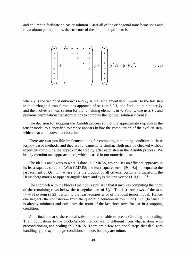
and column to facilitate an easier solution. After all of the orthogonal transformations androw/column permutations, the structure of the simplified problem is
???...????
+
? ? ? · · · ?? ? ?
? · · · ?...
...?
y+
???...????
(sTd0 +‖s‖ ym)2, (3.23)
wherey is the vector of unknowns and ˆym is the last element in ˆy. Similar to the last stepin the orthogonal transformations approach of section 3.2.1, one finds the minimizer ˆym
and then solves a linear system for the remaining elements in ˆy. Finally, one usesVm andprevious permutations/transformations to compute the optimal solutionx from y.
The decision for stopping the Arnoldi process so that the approximate step solves thetensor model to a specified tolerance appears before the computation of the explicit step,which is at an inconvenient location.
There are two possible implementations for computing a stopping condition in theseKrylov-based methods, and they are fundamentally similar. Both may be checked withoutexplicitly computing the approximate stepdm after each step in the Arnoldi process. Webriefly mention one approach here, which is used in our numerical tests.
The idea is analogous to what is done in GMRES, which uses an efficient approach inits least-squares solution. With GMRES, the least-squares error‖b−Ax‖2 is equal to thelast element ofQe1‖b‖, whereQ is the product of all Givens rotations to transform theHessenberg matrix to upper triangular form ande1 is the unit vector(1,0,0, . . .)T .
The approach with the block-3 method is similar in that it involves computing the normof the remaining rows below the triangular part ofHm. The last four rows of them×(m+ 3) system (3.23) pertain to the least-squares error of the local tensor model. Hence,one neglects the contribution from the quadratic equation in rowm of (3.23) (because itis already minimal) and calculates the norm of the last three rows for use in a stoppingcondition.
As a final remark, these local solvers are amenable to preconditioning and scaling.The modifications to the block-Arnoldi method are no different from what is done withpreconditioning and scaling in GMRES. There are a few additional steps that deal withhandlingsk andak in the preconditioned mode, but they are minor.
40
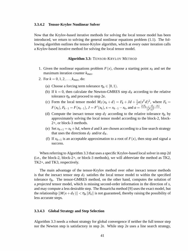
3.3.4.2 Tensor-Krylov Nonlinear Solver
Now that the Krylov-based iterative methods for solving the local tensor model has beenintroduced, we return to solving the general nonlinear equations problem (1.1). The fol-lowing algorithm outlines the tensor-Krylov algorithm, which at every outer iteration callsa Krylov-based iterative method for solving the local tensor model.
Algorithm 3.3: TENSOR-KRYLOV METHOD
1. Given the nonlinear equations problemF(x), choose a starting pointx0 and set themaximum iteration counterkmax.
2. For k = 0,1,2, . . . ,kmax, do:
(a) Choose a forcing term toleranceηk ∈ [0,1).(b) If k = 0, then calculate the Newton-GMRES stepdN according to the relative
toleranceηk and proceed to step 2e.
(c) Form the local tensor modelMT(xk + d) = Fk + Jd+ 12a(sTd)2, whereFk =
F(xk), Fk−1 = F(xk−1), J = F ′(xk), s= xk−1−xk, anda = 2(Fk−1−Fk−Js)(sTs)2 .
(d) Compute the inexact tensor stepdT according to the relative toleranceηk byapproximately solving the local tensor model according to the block-2, block-2+, or block-3 methods.
(e) Setxk+1 = xk+λd, whered andλ are chosen according to a line search strategythat uses the directionsdT and/ordN.
(f) If xk+1 is an acceptable approximation to a root ofF(x), then stop and signal asuccess.
When referring to Algorithm 3.3 that uses a specific Krylov-based local solver in step 2d(i.e., the block-2, block-2+, or block-3 methods), we will abbreviate the method as TK2,TK2+, and TK3, respectively.
The main advantage of the tensor-Krylov method over other inexact tensor methodsis that the inexact tensor stepdT satisfies the local tensor model to within the specifiedtoleranceηk. The tensor-GMRES method, on the other hand, computes the solution ofa projectedtensor model, which is missing second-order information in the direction ofs,and may compute a less desirable step. The Bouaricha method [9] uses the exact model, butthe relationship‖M(x+dT)‖< ηk‖Fk‖ is not guaranteed, thereby raising the possibility ofless accurate steps.
3.3.4.3 Global Strategy and Step Selection
Algorithm 3.3 needs a robust strategy for global convergence if neither the full tensor stepnor the Newton step is satisfactory in step 2e. While step 2e uses a line search strategy,
41
a trust region strategy is still viable, albeit less straightforward. Here we discuss detailsregarding a line search implementation in the tensor-Krylov method.
The standard tensor line search of [57] and the TENSOLVE line search of [9, 10] arestraightforward applications of backtracking along the tensor step, if it is a descent direc-tion, or otherwise along the Newton direction. The curvilinear line search implementationin [4] requires a little adaptation. The curvilinear stepdT(λ) is the solution of the mod-ified tensor modelλF + Jd+ 1
2a(sTd)2, whereλ is the line search parameter. Thus, inthe tensor-Krylov algorithm, the local tensor model is likewise changed and recomputed.Fortunately, the scalarλ is carried through the process in a straightforward manner, irre-spective of method. Specific details are covered in [2] Because the curvilinear line searchfor tensor methods has posted encouraging results and has a nice theoretical basis, we willuse this line search implementation in the tensor-Krylov algorithm.
It should be noted that other large-scale tensor methods, such as the tensor-GMRESmethod of Feng and Pulliam [24], could employ the curvilinear line search even thoughthese other methods have subtle differences in calculating an inexact tensor step. This isbecause the curvilinear step is calculated from a simple scalar multiplication of the func-tion value in the local tensor model and may be carried through the algebra of the stepcalculation to arrive at a parametric form of the curvilinear step.
3.4 Modified Bouaricha Method
Tensor methods have a reputation for being difficult to understand and cumbersome toimplement. Our goal was to implement a tensor method for general use at Sandia that waseasy to understand (as far as tensor methods go), computationally efficient, robust on awide range of problems, capable of running in parallel, and capable of using preexistinglinear solvers with all of their advanced features.
Our experience has shown us that we cannot use just any linear solver for the difficultapplications at Sandia. Advanced linear solvers such as AZTEC [64] are needed. Unfor-tunately, these linear solvers are not easily modified and typically do not provide the Hes-senberg matrices and other information needed by the tensor-Krylov and tensor-GMRESmethods. More precisely, the tensor-Krylov methods [2, 3] require their own specializedKrylov-based solver, which prevents them from serious consideration. Tensor-GMRES[24], while more flexible with its linear solver requirements, still needs the Hessenbergmatrix and orthogonal basis, which are usually not accessible from a standard interface.Bouaricha’s method [9], on the the other hand, is capable of using any stand-alone linearsolver, be it GMRES, TFQMR, BiCGSTAB, etc.
However, in experiments performed in [2], Bouaricha’s method usually lagged in per-formance, sometimes by as much as twice the running time of the other algorithms. Thus,here we propose modifications to Bouaricha’s method [9] that seek to address two aspects
42
of the original algorithm. First, we address a theoretical deficiency that involves neglectinga complicated term for an exact step. Second, Bouaricha’s method suffers from slow con-vergence due to the sequential solution of two linear systems per outer iteration, which wepropose to address with block linear solvers. We describe both of these changes next.
Previously we saw that, when calculating the tensor step, Bouaricha’s method neglectsthe complicated term in (3.11) involvingq(β∗),
(JTk Jk)−1sk
sTk (JT
k Jk)−1skq(β∗). (3.24)
Bouaricha justifies this omission by noting that the term has a considerable computationalcost for large-scale problems and that there appears to be no way to calculate it withouthaving all ofJk available. While it can be proven that the step calculated without (3.24) stillretains the same superlinear convergence properties of a standard tensor method, neglectingthis term means that the resultant step is no longer a minimizer of the local tensor model.We believe there is a better approach than dropping (3.24).
Our modification to Bouaricha’s algorithm approaches the problem from a practicalstandpoint. When the iterates are close to the solution, the tensor model in nearly all caseshas a root. The nonroot cases usually occurs when the solver is far from the real solutionand the solver is taking large steps. In this case, the second-order tensor termak, whichis formed by secant approximation and depends on the step length, is most likely a poorapproximation. Hence, the local model may deviate significantly from the actual function,andMT(xk +d) may no longer have a root.
Intuition tells us that when the local model is significantly wrong, we should backoff and be less aggressive in attempts at modeling the function aroundxk. Thus, one ofour modifications to Bouaricha’s method attenuates the local tensor model by scaling thesecond-order information closer to a linear model (i.e., closer to Newton’s method). Weaccomplish this by multiplying the tensor term12ak(sT
k d)2 by a scalar parameterα:
MT(xk +d) = Fk +Jkd+ 12αak(sT
k d)2.
This parameter is initially set to one, which implies solving the standard tensor model asbefore, but if a real root is not found, then we chooseα ∈ (0,1] such that the model has areal root. This is done easily by forming the parameterized quadratic equation
q(β;α) = 12αsT
k J−1k akβ2 +β+sT
k J−1k Fk. (3.25)
If (3.25) does not have a real root forα = 1, then the value ofα that admits a single realroot is
α =1
4(sTk J−1
k ak)(sTk J−1
k Fk). (3.26)
A second limitation of Bouaricha’s original method is its performance—two linear sys-tems are solved per iteration. As mentioned in section 3.3.2, a clever technique attempts
43
to address this issue by using the previous Newton step as an initial guess to the secondlinear system,Jkw = Fk−1. In practice, this technique does not play a significant role untilthe iterates are very close to the solution, which leaves a lot of early iterations where thealgorithm solves two linear systems with roughly equal work.
To address this, we propose a second modification of using a block linear solver to solvethe two linear systems in tandem. For instance, a block-Krylov method [51] works with ablock of initial vectorsV to produce the block-Krylov subspace
spanV,JV,J2V,J3V, . . .. (3.27)
The block-Arnoldi process creates additional columns of the orthonormal basis for (3.27),with many versions available for implementation. The standard block-Arnoldi procedureworks on a whole blockV ∈Rn×p and addsp vectors—p= 3 in this case—to the subspaceat a time.
Block solvers are more efficient with cache memory than scalar linear solvers solvingmultiple right hand sides [6]. The reason is that, as memory latency costs begin to dominatean algorithm, it becomes more expensive to retrieve a Jacobian matrix from memory. Blocksolvers take advantage of this by multiplying multiple vectors with the parts of the matrixthat reside in cache memory. This extra computation is almost free compared to the timethat the matrix would have to be fetched and pulled through cache memory in subsequentlinear solves with a scalar method.
The option to use a block linear solver may or may not be available, depending onthe availability of a library. The complete algorithm for solving the local model at eachnonlinear iteration is presented below.
Algorithm 4.1: MODIFIED BOUARICHA METHOD
1. If a block solver is available, approximately solve the block system
Jk[dN y] =−[Fk Fk−1]
for dN andy using a block linear solver, such as block GMRES. Otherwise, solveeach system independently using a standard linear solver. The initial guess
y0 =−dNk−1 = J−1k−1Fk−1
may be used for the second right hand side in the system.
2. Form the termw = J−1k ak by using the following relationship:
w = J−1k ak
=2
(sTk sk)2
(J−1k Fk−1−J−1
k Fk−sk)
=2
(sTk sk)2
(−y+dN−sk).
44
3. Form the quadratic equation
q(β;α) = 12αsT
k J−1k akβ2 +β+sT
k J−1k Fk (3.28)
= 12αsT
k wβ2 +β−sTk dN, (3.29)
with α = 1 and find the smallest magnitude real rootq(β;α). If a real root does notexist, then chooseα ∈ (0,1] such that a single real root exists:
α = (3.30)
4. Calculate the tensor step
dT = −J−1k Fk− 1
2J−1k akβ2
∗
= dN− 12αwβ2
∗,
whereβ∗ is a real root of (3.29).
5. Select the next iteratexk+1 using a line search global strategy (as outlined in sec-tion 3.3.4.3).
3.5 Computational Results
This section describes numerical tests aimed at comparing the modified Bouaricha methodwith Newton-GMRES. We provide a limited comparison of the other methods and pri-marily focus on our modified Bouaricha method. Additional numerical tests comparing theother tensor methods may be found in [3, 2], and results on several ill-conditioned problemsare included in [5].
3.5.1 Test Results on Fluid Flow Benchmark Problems
For an initial comparison, we consider a couple of CFD benchmark problems describedin [62] that are used for verification of fluid flow codes and solution algorithms: the 2Dbackward-facing step problem and the 2D thermal convection problem.
We implemented the algorithms in a software package called NOX [41], which is aC++ object-oriented nonlinear solver package being developed at Sandia National Labo-ratories. For objective comparisons, all of the methods, including Newton-GMRES andtensor-GMRES, used the same Arnoldi process (modified Gram–Schmidt) as the tensor-Krylov method. That choice granted us more control over the algorithm and assured us ofa controlled experiment. Thus, the results in this section do not reflect the most efficientand optimized implementations available.
45

We set up the numerical experiments to closely correspond to those in [62], using manyof the same conditions and parameters. A successful termination was declared when bothof the following stopping conditions were satisfied:
‖F(xk)‖ ≤ εF ‖F(x0)‖ (3.31)
and1√n‖Wdk‖< 1, (3.32)
wheren is the total number of unknowns,dk is the full Newton or tensor step, andW is adiagonal scaling matrix with entries
Wii =1
εr |xki |+ εa,
in which xki is theith element of the current solutionxk. We used the same parameters asin [62]: εF = 10−2, εr = 10−3, andεa = 10−8.
In practice, the step length criterion (3.32) is more stringent than (3.31) and is necessaryto resolve finer details of the fluid flow and transport by requiring that eachith element ofthe Newton or tensor step be small relative to its current valuexki . All successful runs,except for two noted below in section 3.5.1.2, satisfied (3.31) with at leastεF = 10−8 andconverged to the same solution. The last several iterations in each run were needed tosatisfy (3.32).
If the test problem required more than 200 nonlinear (outer) iterations or if there wasa line search failure (i.e.,f (xk +λd)≤ f (xk)+αλ∇ f (xk)Td, where f (x)≡ 1
2 ‖F(x)‖2 andα = 10−4, could not be satisfied withλ > 10−12 in at most 40 backtracks), then we declareda failure for the run.
The tests in [62] used a variety of forcing terms, particularly the adaptive forcing termsof Eisenstat and Walker [20]. As mentioned in section 3.3.4.3, more research is neededto determine how best to apply adaptive forcing terms to tensor methods. Consequently,we have used a constant forcing term ofηk = 10−4 in the 2D problems andηk = 10−2
in the 3D problem. As in [62], we allowed the local solver (i.e., GMRES or its tensor-Krylov equivalent) a restart value of 200 with a maximum of 600 total iterations. If thelocal solver did not satisfy the desired tolerance within the 600 iterations, then we used thestep computed thus far and tested for step acceptance with our global strategies. Restartingbecame more of an issue as the problem difficulty increased.
We used an explicit Jacobian, which our PDE code computed efficiently by a com-bination of analytic evaluation and numerical differentiation, and enabled the option formaximum accuracy in the Jacobian. We employed right preconditioning in all cases us-ing an ILUT preconditioner [49], and we performed no variable or function scaling in theproblems. The initial approximation was the zero vector for all cases.
While we recommended using a block linear solver for our modified Bouaricha method,one was not available for these experiments. Belos [22] is a suite of block solvers in
46

the Trilinos software framework [34], but it was not interfaced to NOX in time for theseexperiments. Thus, we have tallied a worst-case type estimate for the method if a blocklinear solver were used. For each nonlinear iteration, we recorded the number of lineariterations for both linear solves. Then we took the larger of the two and added that to ourrunning tally. We believe this is a reasonable estimate for two reasons. First, this numberwould be greater than or equal to the actual number of block iterations because the union ofthe two Krylov subspaces that solve the two right-hand sides in the scalar case is containedwithin the span of the block Krylov subspace generated in this many iterations. Second, thetime per block linear iteration would be just slightly more than a scalar linear iteration dueto the simultaneous computation of matrix-vector products as the matrix is pulled throughcache memory only once [33].
We used a standard backtracking line search procedure for Newton-GMRES and usedthe complete tensor-GMRES algorithm in [24], including their globalization. For thetensor-Krylov methods, we used the curvilinear line search due to favorable theoreticaland performance considerations in [4]. For selecting the line search parameter at each trialstep, we used theλ-halving procedure (dividingλ by two at each inner iteration). Quadraticbacktracking was an option but generally required more iterations and function evaluationsthan λ-halving across all methods in preliminary tests on these problems, so it was notused.
All single processor tests were performed on a dual 3GHz Pentium Xeon desktop com-puter with 2GB of RAM, which was more than sufficient for these problems. However,the computer was not dedicated to these tests, so the timing statistics provided are onlyapproximate and could be off by 10% or more relative to each other. The parallel proces-sor test was performed on a dedicated 16 node/32 processor cluster of 1 GHz Pentium IIIprocessors.
The fluid flow problems are set up using a particular spatial discretization of the gov-erning steady-state transport equations for momentum and heat transfer in flowing fluids.These governing PDEs are given below. The unknown quantities in these equations are thefluid velocity vector (u), the hydrodynamic pressure (P), and the temperature (T).
Conservation of mass: ∇ ·u = 0 (3.33)
Momentum transport: ρ u ·∇u−∇ ·T−ρg = 0 (3.34)
Energy transport: ρCpu ·∇T +∇ ·q = 0 (3.35)
In these equations,g is the gravity vector, andρ andCp are the density and specific heatat constant pressure of the bulk fluid, respectively. The constitutive equations for the stresstensorT and heat fluxq are
T = −PI +µ(∇u+∇uT),q = −κ∇T,
whereµ is the dynamic viscosity andκ is the thermal conductivity of the fluid.
47
The particular spatial discretization of (3.33)–(3.35) that we use is from a finite el-ement reacting flow code called MPSalsa [60] developed at Sandia. MPSalsa generatesan algebraic system of equations by a pressure-stabilized Petrov–Galerkin finite elementformulation of the low Mach number Navier–Stokes equations with heat transport. Thisscheme uses equal-order interpolation of velocity and pressure, and we enabled the optionfor streamline upwinding to limit oscillations due to high grid Reynolds numbers. Sincethe publication of [62], the pressure-stabilized streamline upwinding Petrov–Galerkin for-mulation in MPSalsa has been changed to a Galerkin least squares–type method [59]. Thisstabilization method is slightly less dissipative, and the nonlinear convergence behaviorfor difficult problems can be less robust at higher Reynolds numbers. Consequently, thischange precludes direct comparisons with results in [62].
To complete a problem’s specification, boundary conditions are imposed on the gov-erning PDEs, which we discuss in the subsections that follow. The problems differ only intheir boundary conditions and in whether they use (3.33)–(3.35) or only (3.33)–(3.34). Thenext two subsections describe the test problems and their results.
3.5.1.1 Thermal Convection Problem
This problem consists of the thermal convection (or buoyancy driven) flow of a fluid ina differentially heated square cavity in the presence of gravity. It requires the solutionof (3.33)–(3.35) on the unit square with the following Dirichlet and Neumann boundaryconditions:
T = Tcold, u = 0 at x = 0, (3.36)
T = Thot, u = 0 at x = 1, (3.37)∂T∂y
= 0, u = 0 at y = 0,1. (3.38)
Once the governing equations and boundary conditions are nondimensionalized, two pa-rameters appear: the Prandtl number (Pr) and the Rayleigh number (Ra). In our experi-ments, we fixed Pr = 1 and increased the Rayleigh number from Ra = 104 up to 2×10⁷,which increases the nonlinear effects of the convection terms and makes the solution moredifficult to obtain. The range in [62] is Ra = 103 to 106, but we shifted the range to ex-plore the effectiveness of tensor methods on more difficult problems. We used a 100×100equally spaced mesh, which has 40,804 unknowns. On this size mesh, it is unclear whetherthe choice of Ra> 106 admits a physically accurate and/or stable solution, but we are in-terested only in the relative performance of the numerical methods on this problem, whichremain valid comparisons.
Figure 3.1 shows the overall performance of Newton-GMRES and all of the tensormethods on this problem. As the Rayleigh number increases, Newton-GMRES and tensor-GMRES require increasingly more iterations to solve the problem. For Ra≥ 107, Newton-GMRES fails to solve the problem in 200 iterations. Thus, the trend for Newton-GMRES is
48

a clear degradation in performance as the problem becomes more difficult to solve. Tensor-GMRES is unable to solve the problem for Ra≥ 8× 10⁶. In contrast, the other tensormethods (due in part to the curvilinear line search) are much less affected by the transitionand see a much smaller increase in nonlinear iterations.
104
105
106
107
0
50
100
150
200N
onlin
ear
Itns
2D Thermal Convection Problem
104
105
106
107
0
2
4x 10
4
Arn
oldi
Itns
104
105
106
107
0
2000
4000
Tim
e(se
c)
Rayleigh Number
Newton−GMRESMod. BouarichaTensor−GMRESTK2TK3
Figure 3.1. 2D Thermal convection problem results for Newton-GMRES and all tensor methods.
Figure 3.2 shows just the results for the modified Bouaricha method and Newton-GMRES. The middle plot shows the results of the modified Bouaricha method with a stan-dard linear solver (scalar implementation rather than block). The results are less impressivebut still better than Newton-GMRES on the most difficult problems. As seen in Figure 3.1,other tensor methods perform better in a scalar implementation due to solving only onesystem as opposed to two linear systems.
The bottom plot of Figure 3.2 shows the expected performance of a block linear solverimplementation of the modified Bouaricha method. One block iteration (unit on the y-axis) is just slightly more expensive than an iteration from a scalar implementation. This isbecause the cost of multiplying an extra vector with a sparse Jacobian that already residesin cache memory is small compared to the cost of retrieving the matrix from main memory.
We show similar results in Figure 3.3 for results run on 8 processors of a parallel com-
49
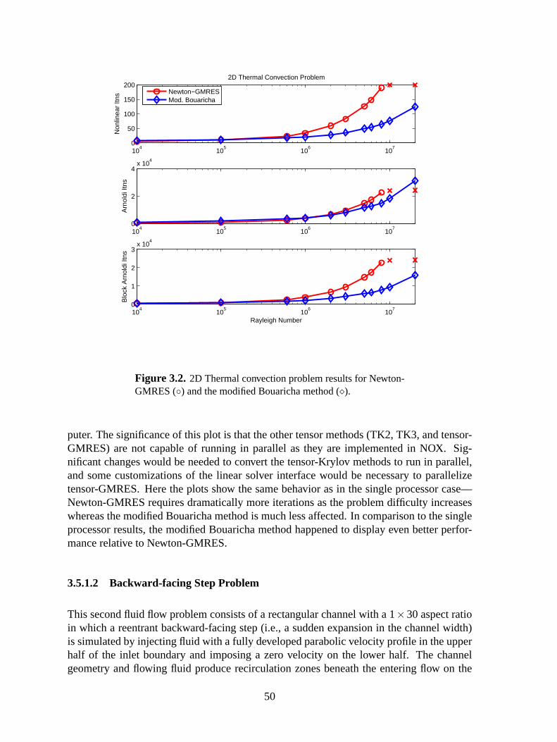
104
105
106
107
0
50
100
150
200
Non
linea
r Itn
s
2D Thermal Convection Problem
104
105
106
107
0
2
4x 10
4
Arn
oldi
Itns
104
105
106
107
0
1
2
3x 10
4
Blo
ck A
rnol
di It
ns
Rayleigh Number
Newton−GMRESMod. Bouaricha
Figure 3.2. 2D Thermal convection problem results for Newton-GMRES () and the modified Bouaricha method ().
puter. The significance of this plot is that the other tensor methods (TK2, TK3, and tensor-GMRES) are not capable of running in parallel as they are implemented in NOX. Sig-nificant changes would be needed to convert the tensor-Krylov methods to run in parallel,and some customizations of the linear solver interface would be necessary to parallelizetensor-GMRES. Here the plots show the same behavior as in the single processor case—Newton-GMRES requires dramatically more iterations as the problem difficulty increaseswhereas the modified Bouaricha method is much less affected. In comparison to the singleprocessor results, the modified Bouaricha method happened to display even better perfor-mance relative to Newton-GMRES.
3.5.1.2 Backward-facing Step Problem
This second fluid flow problem consists of a rectangular channel with a 1×30 aspect ratioin which a reentrant backward-facing step (i.e., a sudden expansion in the channel width)is simulated by injecting fluid with a fully developed parabolic velocity profile in the upperhalf of the inlet boundary and imposing a zero velocity on the lower half. The channelgeometry and flowing fluid produce recirculation zones beneath the entering flow on the
50
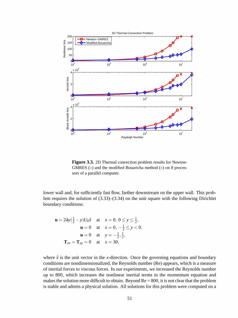
104
105
106
107
0
50
100
150
200
Non
linea
r Itn
s
2D Thermal Convection Problem
104
105
106
107
0
2
4x 10
4A
rnol
di It
ns
104
105
106
107
0
2
4x 10
4
Blo
ck A
rnol
di It
ns
Rayleigh Number
Newton−GMRESModified Bouaricha
Figure 3.3. 2D Thermal convection problem results for Newton-GMRES () and the modified Bouaricha method () on 8 proces-sors of a parallel computer.
lower wall and, for sufficiently fast flow, farther downstream on the upper wall. This prob-lem requires the solution of (3.33)–(3.34) on the unit square with the following Dirichletboundary conditions:
u = 24y(12−y)U0x at x = 0, 0≤ y≤ 1
2,
u = 0 at x = 0, −12 ≤ y < 0,
u = 0 at y =−12, 1
2,
Txx = Txy = 0 at x = 30,
wherex is the unit vector in thex-direction. Once the governing equations and boundaryconditions are nondimensionalized, the Reynolds number (Re) appears, which is a measureof inertial forces to viscous forces. In our experiments, we increased the Reynolds numberup to 800, which increases the nonlinear inertial terms in the momentum equation andmakes the solution more difficult to obtain. Beyond Re = 800, it is not clear that the problemis stable and admits a physical solution. All solutions for this problem were computed on a
51
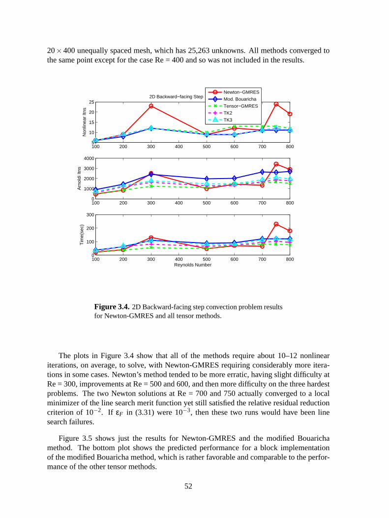
20×400 unequally spaced mesh, which has 25,263 unknowns. All methods converged tothe same point except for the case Re = 400 and so was not included in the results.
100 200 300 400 500 600 700 8005
10
15
20
25
Non
linea
r Itn
s
2D Backward−facing Step
100 200 300 400 500 600 700 8000
1000
2000
3000
4000
Arn
oldi
Itns
100 200 300 400 500 600 700 8000
100
200
300
Tim
e(se
c)
Reynolds Number
Newton−GMRES
Mod. Bouaricha
Tensor−GMRES
TK2
TK3
Figure 3.4.2D Backward-facing step convection problem resultsfor Newton-GMRES and all tensor methods.
The plots in Figure 3.4 show that all of the methods require about 10–12 nonlineariterations, on average, to solve, with Newton-GMRES requiring considerably more itera-tions in some cases. Newton’s method tended to be more erratic, having slight difficulty atRe = 300, improvements at Re = 500 and 600, and then more difficulty on the three hardestproblems. The two Newton solutions at Re = 700 and 750 actually converged to a localminimizer of the line search merit function yet still satisfied the relative residual reductioncriterion of 10−2. If εF in (3.31) were 10−3, then these two runs would have been linesearch failures.
Figure 3.5 shows just the results for Newton-GMRES and the modified Bouarichamethod. The bottom plot shows the predicted performance for a block implementationof the modified Bouaricha method, which is rather favorable and comparable to the perfor-mance of the other tensor methods.
52
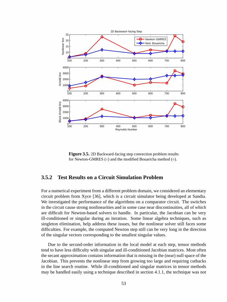
100 200 300 400 500 600 700 8005
10
15
20
25
Non
linea
r Itn
s
2D Backward−facing Step
100 200 300 400 500 600 700 8000
1000
2000
3000
4000
Arn
oldi
Itns
100 200 300 400 500 600 700 8000
1000
2000
3000
4000
Blo
ck A
rnol
di It
ns
Reynolds Number
Newton−GMRES
Mod. Bouaricha
Figure 3.5.2D Backward-facing step convection problem resultsfor Newton-GMRES () and the modified Bouaricha method ().
3.5.2 Test Results on a Circuit Simulation Problem
For a numerical experiment from a different problem domain, we considered an elementarycircuit problem from Xyce [36], which is a circuit simulator being developed at Sandia.We investigated the performance of the algorithms on a comparator circuit. The switchesin the circuit cause strong nonlinearities and in some case near discontinuities, all of whichare difficult for Newton-based solvers to handle. In particular, the Jacobian can be veryill-conditioned or singular during an iteration. Some linear algebra techniques, such assingleton elimination, help address these issues, but the nonlinear solver still faces somedifficulties. For example, the computed Newton step still can be very long in the directionof the singular vectors corresponding to the smallest singular values.
Due to the second-order information in the local model at each step, tensor methodstend to have less difficulty with singular and ill-conditioned Jacobian matrices. Most oftenthe secant approximation contains information that is missing in the (near) null space of theJacobian. This prevents the nonlinear step from growing too large and requiring cutbacksin the line search routine. While ill-conditioned and singular matrices in tensor methodsmay be handled easily using a technique described in section 4.1.1, the technique was not
53

implemented here. Instead, we tested the pure performance of a tensor method versusNewton’s method.
Because circuit simulation problems are very difficult for standard nonlinear solvers,tuning is necessary to avoid catastrophic failures and/or achieve satisfactory performance.Because tuning is usually problem specific, it is not knowna priori which set of parameterswill work the best on a particular problem. Thus, we chose the conditions of this experimentto mimic this idea of parameter tuning. One often tries different global strategies and/orparameters to see what works best in a trial-and-error fashion. Here we run each algorithmwith the same solver options and parameters (linear solver tolerance, full step vs. globalstrategy, etc.) and compare their performance for that run only. Because different parametersets affect the algorithms differently, we are looking for the algorithm that has the bestaverage performance over all parameter sets.
Figure 3.6 shows a binary comparison over fifteen runs with different algorithmic tun-ing parameters. The same set of parameters are used for both algorithms for that particularrun. In the plot we record the logarithm (base 2) of the ratio of nonlinear iterations of New-ton to tensor. The resulting plot shows which method performed better and by how much.Blue bars extending above zero show the extent to which the tensor method was better. Onaverage, the modified Bouaricha method converged in 39% fewer nonlinear iterations thanNewton-GMRES.
Figure 3.7 takes the same results and shows the binary comparison for execution time.On average, the modified Bouaricha method converged in 10% less time than Newton-GMRES. This is due once again to the fact that two linear systems are being solved pernonlinear iteration in the Bouaricha method. If a block linear solver were used to solve thetwo linear systems simultaneously, then each nonlinear iteration would take just slightlymore time than Newton’s method, and this plot would look more like Figure 3.6.
3.6 Discussion
The results of the fluid flow problems are encouraging for our modified Bouaricha tensormethod. They show a preliminary indication that the modified Bouaricha method is morerobust and oftentimes more efficient than standard Newton-GMRES. In general, the ten-sor method would perform on par with Newton-GMRES on the easier problems (lowerRayleigh or Reynolds numbers), but as the difficulty increased, the modified Bouarichamethod would outperform Newton-GMRES. This general trend is seen also with the othertensor methods to varying degrees; see [3].
Part of the success is due to the curvilinear line search, which produces a trial step thathas a direction in the span of the Newton step and tensor step and that reduces to the Newtondirection asλ→ 0, which is a descent direction on the merit function. In a separate study ofline search procedures for tensor methods [4], it was found that the curvilinear line search
54

1 2 3 4 5 6 7 8 9 10 11 12 13 14 15−1
−0.5
0
0.5
1
1.5
2
Run
Per
form
ance
rat
io
Nonlinear Iterations
Figure 3.6. Log-ratio of the number of nonlinear iterations onthe Xyce comparator circuit problem for the following methods:Newton-GMRES and the modified Bouaricha method. Red barsextending below zero favor Newton-GMRES and blue bars extend-ing above zero favor the tensor method.
was the most robust and efficient. In many of the numerical experiments, Newton-GMREShad several line search failures, which are more catastrophic than exceeding the maximumiteration limit because the algorithm cannot make forward progress. The second-order in-formation in the tensor model tends to provide a correction to the Newton step in difficultareas, such as bogging down in a line search, that helps the tensor method “escape” faster.Coincidentally, the accuracy of this second-order information increases during difficult re-gions because, as the line search cuts the step back, the secant approximation in the tensormethod becomes more accurate.
Tensor methods are especially effective at solving large-scale problems that possessJacobians at the solution that are highly ill-conditioned or singular. For theoretical reasons,algorithms based on Newton’s method exhibit very slow convergence on such problems.In the next chapter, we discuss a technique that allows tensor methods to deal with highlyill-conditioned or singular Jacobians during the iterative process.
From our experience with Xyce, tensor methods perform modestly on circuit simula-tion problems, but our observation is that tuning algorithm parameters is a key ingredient tosuccess on these types of problems. In addition, very ill-conditioned and singular Jacobian
55

1 2 3 4 5 6 7 8 9 10 11 12 13 14 15−1
−0.5
0
0.5
1
1.5
2
Run
Per
form
ance
rat
io
Time
Figure 3.7. Log-ratio of execution time on the Xyce comparatorcircuit problem for the following methods: Newton-GMRES andthe modified Bouaricha method. Red bars extending below zerofavor Newton-GMRES and blue bars extending above zero favorthe tensor method.
matrices frequently turn up in these problems. Ultimately, this causes problems for New-ton’s method, but it also caused problems for our implementation of Bouaricha’s method.The reason is that we were still solving two linear systems with this matrix. When the Ja-cobian was ill-conditioned, then the two solutions were accurate only to a limited numberof digits (which depends on the condition number). The tensor step is formed from a linearcombination of these two vectors of limited accuracy, and so some of the significant digitsmay be lost, yielding a potentially spurious step.
The next chapter discusses a technique to avoid such difficulties associated with ill-conditioned and (mildly) singular matrices. Unfortunately, we were not able to implementthis technique for testing on this class of difficult problems. We would expect to see betterperformance provided that the rank of the Jacobian is (or near)n−1. If the rank deficiencyis greater, then a higher-order tensor term should be computed to account for the extramissing information in the null space. Following the paradigm outlined in the next chapter,additional rank-1 matrices may be added to the Jacobian to make it well-conditioned. Withthis approach, we would expect to see a more robust and stable algorithm for dealing withcircuit simulation problems.
56

There are several research questions left at this point to explore. We mention two fu-ture extensions here. First, adaptive forcing terms like the form by Eisenstat and Walker[20] may help improve robustness. Second, there is still the question of accuracy ofβ as afunction of linear solver toleranceη. If the two linear subproblems are solved very approx-imately, then it is possible that a large value ofβ may be calculated, which could undulybias the tensor correction and yield a step far from the Newton direction.
57
Chapter 4
Turning Point Algorithm
In this chapter, we present research on a modified turning point algorithm that works withill-conditioned and singular Jacobians. We first describe an approach that tensor methodsmay use to deal with singular and ill-conditioned Jacobian matrices. We then extend thatidea to a general linear system and apply it to a turning point identification algorithm.
To be consistent with previous chapters, we will keep the subscriptk when discussingthe tensor model at iterationk in the nonlinear solver. Later in this chapter when we aredealing strictly with a local model at the same iterationk, we will drop the subscriptk onJk, Fk, ak, andsk.
4.1 Singular and Ill-conditioned Jacobians
4.1.1 Tensor Methods
Tensor methods [57] incorporate second-order information in a localized model about somecurrent pointxk:
MT(xk +d) = Fk +Jkd+ 12Tkdd, (4.1)
whereTk ∈ Rn×n×n holds some second-order information computed from a secant approx-imation; see section 3.2.1. Unlike local models that are strictly linear, (4.1) can still have asingle real root even if the Jacobian is singular, provided thatTk contains information thatis missing in the null space ofJk. The standard approach for solving the model in this caseis to use orthogonal transformations, as outlined in section 3.2.1.
Briefly, the solution of a rank-1 tensor model can be reduced to the solution of a systemof q quadratic equations in 1 unknown, plus the solution of a system ofn−q linear equa-tions inn−1 unknowns; see [57]. Most oftenq = 1, but a singular Jacobian with a rankdeficiency greater than one will makeq > 1. In this case, the number of linear equations
58
is decreased by this rank deficiency from the normal case, and the number of quadraticequations is increased correspondingly, leaving the number of variables in each systemunchanged.
The other approach for solving a rank-1 tensor model, what we will call the “reductionmethod” and is used in Bouaricha’s method [9], solves two linear systems withJk to forma reduced system of quadratic equations. Clearly, ifJk is singular, then the linear systemsare unsolvable and this method breaks down.
We outline an approach that makes the reduction method feasible for a singular (orill-conditioned) Jacobian under mild conditions. Once again, we will concentrate on therank-1 tensor model formed by a secant approximation as derived in section 3.2.1:
MT(xk +d) = Fk +Jkd+ 12ak(sT
k d)2. (4.2)
In the nonsingular case, the solution to (4.2) is found by solving two linear systems withFk
andak (or Fk−1 as we have shown before) as right hand sides. Then we form the quadraticequation
q(β)≡ sTk J−1
k Fk +β+ 12sT
k J−1k akβ2
solve for the smallest magnitude real root, which we callβ∗. For this section, we consideronly the case of real roots; see section 3.2.1 for the minimizing case. Then the solution to(4.2) is
dT =−J−1k Fk− 1
2J−1k akβ2
∗.
Clearly, this method breaks down whenJk is singular, but there can be problems whenJk isill-conditioned, too. These problems are caused by the accuracy of the two linear solutionsand the fact that they are added together. If they are of opposite signs, then there may becancellation of the accurate digits, leaving one with fewer (or no) accurate digits.
The approach to solving (4.2) whenJk is singular or ill-conditioned deals with modify-ing the system such that the underlying system is unchanged. We start by adding a cleverform of zero,[aksT
k d−aksTk d], and rearrange terms.
0 = Fk +Jkd+ 12ak(sT
k d)2
0 = Fk +Jkd+ 12ak(sT
k d)2 +[aksTk d−aks
Tk d]
0 = Fk +(Jk +aksTk )d+ 1
2ak(sTk d)2−aks
Tk d
0 = Fk + Jkd+ 12ak(sT
k d)2−aksTk d (4.3)
The matrixJk ≡ (Jk + aksTk ) is the original Jacobian plus a rank-1 matrix,aksT
k . It is thisrank-1 matrix that makesJk better conditioned thanJk. We will comment later on condi-tions that make it so.
We continue by noting that (4.3) may be simplified further by “completing the square”of the last two terms. By adding another clever form of zero, this time[1
2ak− 12ak], the last
59
two terms may be collected and written as a square:
0 = Fk + Jkd+ 12ak(sT
k d)2−ak(sTk d)+ [1
2ak− 12ak],
0 = Fk− 12ak + Jkd+ 1
2ak(sTk d)2−ak(sT
k d)+ 12ak,
0 = Fk + Jkd+ 12ak(sT
k d−1)2. (4.4)
Equation (4.4) is identical to our original system (4.2) because we have added nothing butzeros to the system. Indeed, using these definitions,
Jk ≡ Jk +aksTk ,
Fk ≡ Fk− 12ak,
β∗ ≡ sTk dT −1,
the model in (4.2) may be written as
MT(xk +d) = Fk + Jkd+ 12akβ2. (4.5)
Because (4.5) is identical to (4.2) in form, we may solve (4.5) using the reductionmethod. That is, we form the quadratic equation
q(β)≡ sTk Jk−1Fk + β+ 1
2sTk Jk−1akβ2
and find its smallest magnitude real rootβ∗. Then the root of both (4.2) and (4.5) is givenby
dT =−Jk−1Fk− 1
2Jk−1akβ2
∗.
We now discuss the conditions that makeJk have a lower condition number thanJk. Westart our analysis with the singular value decomposition (SVD) ofJk. Let Jk = UΣVT =∑n
i=1uiσivi , whereU andV are unitary matrices with orthogonal columns andΣ is a diago-nal matrix of singular valuesσ1≥ σ2≥ ·· · ≥ σn≥ 0. The condition number ofJk is givenby κ(Jk) = σ1
σn. Thus, if the smallest singular valueσn is zero, then the matrix is singular
andκ(Jk) = ∞.
The rank-1 matrixaksTk that is added toJk will add some amount to one or more of the
singular values ofJk. If ak is a multiple ofun andsk is a multiple ofvn, then the contributionis purely in the last singular value and the condition number of
Jk =max(σ1,uT
n aksTk vn)
min(σn−1,uTn aksT
k vn).
In practice, it is never the case thatak is a multiple ofun, but there is some theory forsk.
An ideal tensor method [23] would construct the tensor termTk from exact secondderivatives as well as the null space ofJk. More precisely,sk would correspond tovn, the
60

least singular vector ofJk, andak would beF ′′(xk)vnvn. Normally, this is too expensiveto compute so a practical approach uses a secant approximation to obtainsk andak. Thechoice ofsk = xk− xk−1 approximately lies in the direction ofvn because the differencebetween two consecutive iterates is likely to be along the null space when consecutiveiterates are in the funnel around the null space near the solution [23, 24]. Close to thesolution, the vectorF ′′(xk)vnvn is likely to be approached by ourak in (3.4).
Thus, one approximately hassk proportional tovn but no such condition onak. ProvidedthatuT
n aksTk vn 6= 0, then the condition number ofJ will no longer be infinite. In effect, the
rank-1 matrix boosts the smallest singular value ofJk, which makesJk nonsingular. Forill-conditioned matrices, it is likely, but not guaranteed, that the condition number willimprove.
4.1.2 General Linear Systems
We now apply this technique to general linear systems that are very ill-conditioned. Inkeeping with our notation from all previous sections on nonlinear equations, where thematrix is a Jacobian, we write the linear system asJx= b instead of the more traditionalAx= b. For this discussion we assume thatJ ∈ Rn×n is either singular with rankn−1 orvery ill-conditioned with the smallest singular valueσn σn−1. However, the approachoutlined here is generalizable to a larger rank-deficiency.
The approach to solving (4.2) whenJ is singular or ill-conditioned is similar to theapproach above. It is actually a variation of the Sherman-Morrison-Woodbury formula[27]. A similar but unrelated idea is contained in the Interlocking Eigenvalue Lemma dueto Loewner (stated in [42]), which relates the eigenvalues of a symmetric matrixA to theeigenvalues ofA plus a rank-1 matrixeieT
i , whereei is theith unit vector.
We start by choosing two vectorsu,v∈Rn such that their inner product with the small-est left and right singular vectors ofJ (resp.) is nonzero. For simplicity we’ll assume thatu,v have unit length. Ideally we would likeu = un andv = vn. We also choose a scalefactorα and form the rank-1 matrixαuvT . Then we take its product with the unknownx,add it to both sides of the linear equation, rearrange terms, and solve forx:
Jx = b,
Jx+αuvTx = b+αuvTx,
(J+αuvT)x = b+αuvTx,
Jx = b+αuvTx,
x = J−1b+αJ−1u(vTx).
BecauseuvT provides information in the smallest singular vectors ofJ, the matrixJ ≡(J+ αuvT) is nonsingular and hopefully better conditioned thanJ. Later, we will discussissues for choosingα, u, andv to makeJ better conditioned thanJ.
61
Now, in a manner similar to the reduction method for solving a rank-1 tensor model,we take the inner product of both sides withv and solve for the unknownβ≡ vTx,
vTx = vT J−1b+αvT J−1u(vTx)
β ≡ vTx =vT J−1b
1−αvT J−1u
Finally, the solution to the linear system is given by
x = J−1b+αJ−1uβ (4.6)
where
J ≡ J+αuvT ,
β ≡ vT J−1b
1−αvT J−1u.
Some comments are in order. First, as mentioned above, the vectorsu andv must notbe orthogonal to the smallest singular vectors ofJ. If they are orthogonal, thenJ is nobetter conditioned thanJ. Second, it is best to haveu andv close toun andvn. Third, thescaling factorα is used to scale the contribution of this matrix so that the smallest singularvalue ofJ is boosted betweenσ1 andσn−1. Fourth, this technique cannot be used to solveJx= b if J is singular. For such a system, there is either no solution or an infinite numberof solutions. However, even ifb is in the range ofJ, the denominator ofβ would be zero.Last, this technique involves the solution of two linear systems with the same matrixJ butdifferent right hand sides,b andu. The cost associated with solving two systems may beamortized over a single loop with block linear solvers.
The benefit of this technique is that many iterative methods are adversely affected by alarge condition number of the matrix. Hence, preconditioning techniques have been devel-oped to address these issues with linear systems and to help speed up convergence. Thistechnique is a different approach that may address many of the same issues.
4.2 Turning Point Identification
We turn our attention to an application of this technique for solving ill-conditioned linearsystems. In particular, the identification of turning points in physical systems involvesfinding the point on a curve of a family of solutions to a physical problem such that theJacobian matrix has rankn−1.
More precisely, we are interested in a general physical problem described by the systemof nonlinear equationsF(x,λ), wherex is the state vector andλ is a parameter. We may
62
trace out a family of solutions tox for a range of values ofλ. If the curve turns back onitself, then there is a critical valueλ∗ that has only one solution. On one side ofλ∗ there aretwo solutions and on the other side there are no solutions toF(x,λ). The pointλ∗ is calleda turning point, and the Jacobian at this point is singular with rank deficiency of one.
A system of nonlinear equations that explicitly defines a turning point may be writtendown and solved:
F(x,λ) = 0, (4.7)
Jv = 0, (4.8)
φTv = 1. (4.9)
The first equation is the state equation of the physical problem. The second equation spec-ifies that the Jacobian ofF(x,λ) with respect tox is singular with a null vectorv. The lastcondition is a scalar equation to keepv away from the trivial solution ofv = 0. This is asystem of 2n+1 equations, which may be solved by Newton’s method:
J 0 ∂F∂λ
∂(Jv)∂x J ∂(Jv)
∂λ0 φT 0
∆x∆v∆λ
=−
FJv
φTv−1
(4.10)
4.2.1 Bordered Algorithm
In practice, it is difficult to solve (4.7)–(4.9) strictly by Newton’s method because someentries of the full Jacobian matrix are difficult to calculate. We discuss a practical algorithmin LOCA [54, 55] for solving this system. It is called a bordered algorithm, and it may bederived from a block elimination procedure. We provide a brief outline of the algorithmhere; for more details see [54, 55];
The bordered algorithm involves four intermediate solves with the Jacobian matrix:
Ja = −F,
Jb = −∂F∂λ
,
Jc = −∂(Jv)∂x
a,
Jd = −∂(Jv)∂x
b− ∂(Jv)∂λ
.
63

Then we may compute the Newton step with the four solutions toa,b,c, andd:
∆λ =1−φTc
φTd∆x = a+∆λb
∆v = c+∆λd−v
The JacobianJ grows more ill-conditioned and eventually singular as we approach theturning point, but the(2n+1)× (2n+1) “system” Jacobian in (4.10) remains nonsingular.Because there are four solves with an ill-conditioned matrix that is being driven to a sin-gularity, the linear combination of these four solutions to form the Newton step would beincreasingly inaccurate.
4.2.2 Modified Bordered Algorithm
To address this issue of an increasingly ill-conditioned system, we propose solving the fourlinear systems using the approach outlined in section 4.1.2. At the current stage of thisresearch, this technique only works with an iterative solver that solves each system onlyapproximately.
The approach involves adding a nonzero vector to both sides of the Newton equation tofacilitate a way to improve the conditioning of the matrix (the Jacobian) appearing in thelinear subproblems:uvT∆x
uvT∆v0
+
J 0 ∂F∂λ
∂(Jv)∂x J ∂(Jv)
∂λ0 φT 0
∆x∆v∆λ
=−
FJv
φTv−1
+
uvT∆xuvT∆v
0
. (4.11)
The solution to this problem is the same as if it were calculated by standard Newton’smethod.
Using the same bordering algorithm approach, we may solve (4.11) by solving smallersubproblems with the same matrix. That is, we solve the four linear systems
Ja = −F +uvTa
Jb = −∂F∂λ
+uvTb
Jc = −∂(Jv)∂x
a+uvTc
Jd = −∂(Jv)∂x
b− ∂(Jv)∂λ
+uvTd
for a,b,c,d, where J ≡ J + uv. In this case we letv equal the current estimate of thenull space vector being solved for in the turning point problem, and we chooseu to be a
64

scaled approximation to the smallest left singular vector ofJ. We use the approximationu= αJv/‖Jv‖, whereα is a scaling factor to make the condition number ofJ be acceptable.The actual value ofα is not important so long as it is not too high and not too low. Ideally,α should be between the largest singular value ofJ and second smallest singular value ofJ, i.e.,σ1 > α > σn−1.
We point out that for each linear system, the solution is implicitly defined, and one mustcalculate its solution in the manner of section 4.1.2. That is, to solve fora,b,c,d, one alsoneeds the solution toJ−1u, or at least an approximation. Thus, this approach requires fivelinear solves per Newton step.
Once the solutions fora,b,c,d have been computed, one forms the Newton step in thestandard way:
∆λ =1−φTc
φTd,
∆x = a+∆λb,
∆v = c+∆λd−v.
As a final remark, we consider why this technique works. We mentioned in the be-ginning that this technique is only useful with iterative solvers that approximately solve asystem to a specified tolerance. It has not been fully analyzed why this is the case, but it isrelated to the solver tolerance. The solution to each linear system computed by the modifiedmethod is no more accurate than a standard solution. Thus, as the solver approaches theturning point, each individual solution toa,b,c,d is increasingly less accurate. However,the contribution byJ−1u is computed separately and used in each system. Hence, when∆λ,∆x, and∆v are computed, it is believed that the numerical error related to the null spacedirection cancels out, leaving an accurate Newton step.
4.3 Computational Results
This section describes a numerical experiment aimed at comparing the modified turningpoint method with the original bordering method used in LOCA [54, 55]. We use bothapproaches to solve for the turning point in the Bratu problem. The conclusions fromthese results extend to other types turning point identification problems that we tested. Weperformed all experiments in MATLAB .
The Bratu problem is a simplified model for nonlinear diffusion phenomena occurring,for example, in semiconductors and combustion, where the source term is related to theArrhenius law for modeling exothermic reactions. The following version is taken from theset of nonlinear model problems collected by More [43]. The problem is the nonlinear
65
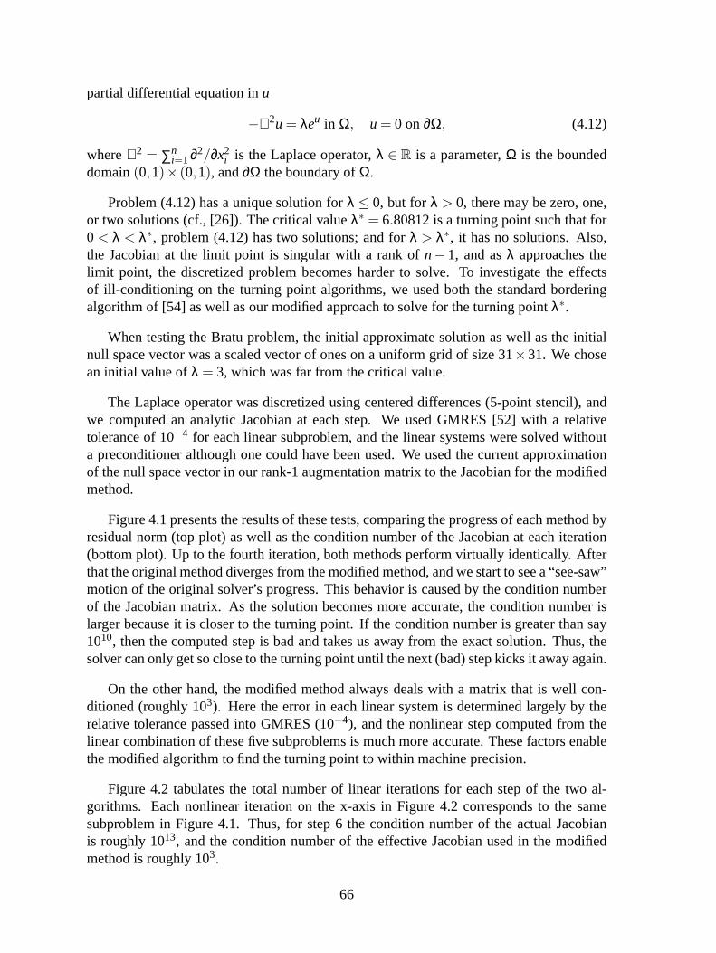
partial differential equation inu
−∇2u = λeu in Ω, u = 0 on∂Ω, (4.12)
where∇2 = ∑ni=1∂2/∂x2
i is the Laplace operator,λ ∈ R is a parameter,Ω is the boundeddomain(0,1)× (0,1), and∂Ω the boundary ofΩ.
Problem (4.12) has a unique solution forλ ≤ 0, but forλ > 0, there may be zero, one,or two solutions (cf., [26]). The critical valueλ∗ = 6.80812 is a turning point such that for0 < λ < λ∗, problem (4.12) has two solutions; and forλ > λ∗, it has no solutions. Also,the Jacobian at the limit point is singular with a rank ofn− 1, and asλ approaches thelimit point, the discretized problem becomes harder to solve. To investigate the effectsof ill-conditioning on the turning point algorithms, we used both the standard borderingalgorithm of [54] as well as our modified approach to solve for the turning pointλ∗.
When testing the Bratu problem, the initial approximate solution as well as the initialnull space vector was a scaled vector of ones on a uniform grid of size 31×31. We chosean initial value ofλ = 3, which was far from the critical value.
The Laplace operator was discretized using centered differences (5-point stencil), andwe computed an analytic Jacobian at each step. We used GMRES [52] with a relativetolerance of 10−4 for each linear subproblem, and the linear systems were solved withouta preconditioner although one could have been used. We used the current approximationof the null space vector in our rank-1 augmentation matrix to the Jacobian for the modifiedmethod.
Figure 4.1 presents the results of these tests, comparing the progress of each method byresidual norm (top plot) as well as the condition number of the Jacobian at each iteration(bottom plot). Up to the fourth iteration, both methods perform virtually identically. Afterthat the original method diverges from the modified method, and we start to see a “see-saw”motion of the original solver’s progress. This behavior is caused by the condition numberof the Jacobian matrix. As the solution becomes more accurate, the condition number islarger because it is closer to the turning point. If the condition number is greater than say1010, then the computed step is bad and takes us away from the exact solution. Thus, thesolver can only get so close to the turning point until the next (bad) step kicks it away again.
On the other hand, the modified method always deals with a matrix that is well con-ditioned (roughly 103). Here the error in each linear system is determined largely by therelative tolerance passed into GMRES (10−4), and the nonlinear step computed from thelinear combination of these five subproblems is much more accurate. These factors enablethe modified algorithm to find the turning point to within machine precision.
Figure 4.2 tabulates the total number of linear iterations for each step of the two al-gorithms. Each nonlinear iteration on the x-axis in Figure 4.2 corresponds to the samesubproblem in Figure 4.1. Thus, for step 6 the condition number of the actual Jacobianis roughly 1013, and the condition number of the effective Jacobian used in the modifiedmethod is roughly 103.
66
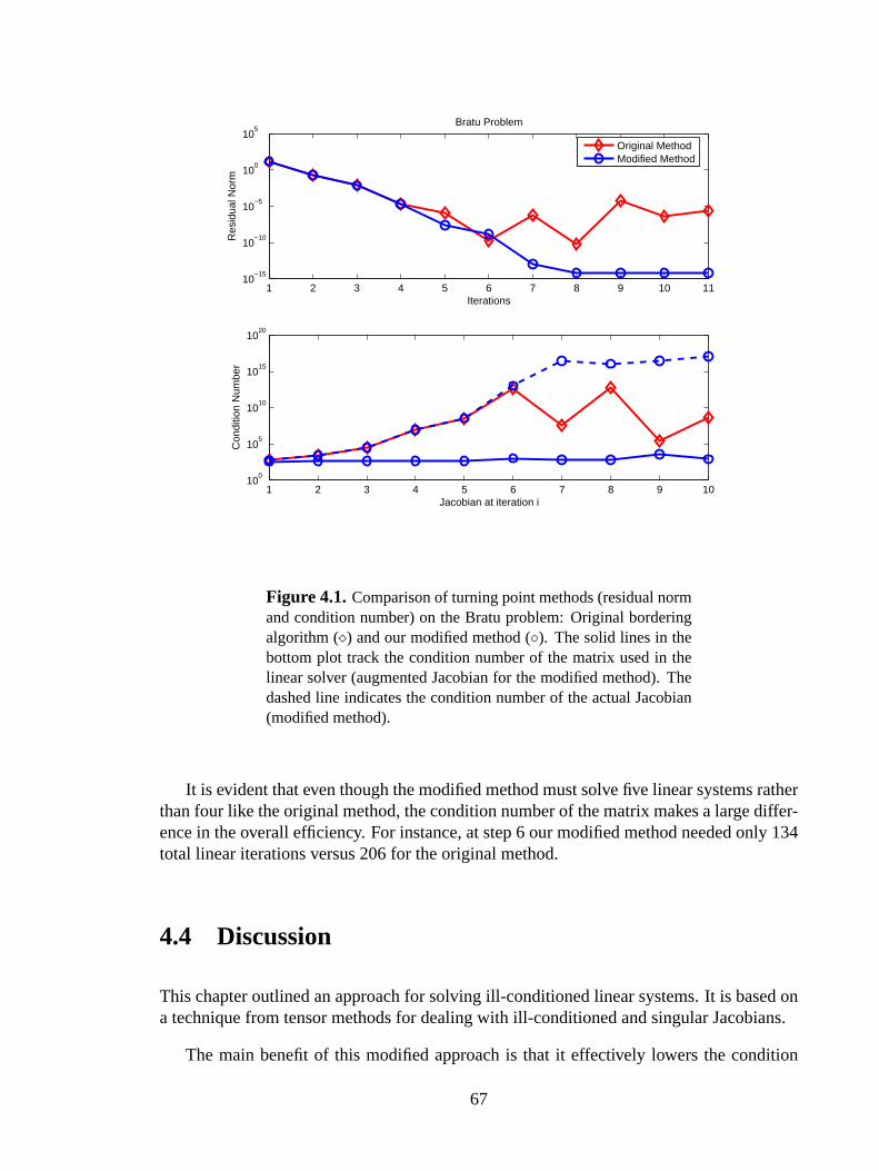
1 2 3 4 5 6 7 8 9 10 1110
−15
10−10
10−5
100
105
Bratu Problem
Res
idua
l Nor
m
Iterations
1 2 3 4 5 6 7 8 9 1010
0
105
1010
1015
1020
Con
ditio
n N
umbe
r
Jacobian at iteration i
Original MethodModified Method
Figure 4.1. Comparison of turning point methods (residual normand condition number) on the Bratu problem: Original borderingalgorithm () and our modified method (). The solid lines in thebottom plot track the condition number of the matrix used in thelinear solver (augmented Jacobian for the modified method). Thedashed line indicates the condition number of the actual Jacobian(modified method).
It is evident that even though the modified method must solve five linear systems ratherthan four like the original method, the condition number of the matrix makes a large differ-ence in the overall efficiency. For instance, at step 6 our modified method needed only 134total linear iterations versus 206 for the original method.
4.4 Discussion
This chapter outlined an approach for solving ill-conditioned linear systems. It is based ona technique from tensor methods for dealing with ill-conditioned and singular Jacobians.
The main benefit of this modified approach is that it effectively lowers the condition
67
1 2 3 4 5 6 7 8 9 100
50
100
150
200
250
Tot
al L
inea
r Ite
ratio
ns
Iteration
Original Method
Modified Method
Figure 4.2. Comparison of turning point methods (total lineariterations per step) on the Bratu problem: Original bordering algo-rithm () and our modified method ().
number of the matrix used in a linear solver. For iterative solvers, such as GMRES [52],the distribution of eigenvalues of the matrix (and consequently its condition number) playsan important role in determining how many iterations are necessary to reach convergence[28]. From our experience, as the condition number increases, the number of iterationsnecessary to satisfy a fixed tolerance also increases. Thus, lowering the condition numberfrom say 1012 to 103 can improve the performance of an iterative solver. In a similarapproach, preconditioning techniques attempt to change the linear system to one that iscloser toIx = A−1b so that the eigenvalues are clustered around one, which also makes thematrix better conditioned.
The modified approach has two principal disadvantages, namely that two linear systemsmust be solved and that it may be difficult to determine an appropriate rank-1 matrix for ageneral problem. The first disadvantage may be mitigated through the use of block linearsolvers.
More research is needed to determine the viability of this approach in practical applica-tions. We have described one application by applying it to the turning point identificationalgorithm, which conveniently computes the null vector.
68
Chapter 5
Summary
The first objective of our research was to investigate Broyden’s method for use in large-scale simulations. We implemented a parallel version and evaluated its applicability andperformance on reacting flow problems and circuit simulation problems. The importantfinding was that Broyden’s method could be used as a replacement for Newton’s methodwhen the Jacobian required for Newton’s method either could not be evaluated or was inac-curate. In this case, the rank-1 update vectors could approximate the missing informationas the iteration sequence progressed. This application of Broyden’s method can be seen asa competitor to the Jacobian-free Newton-Krylov method since neither require a Jacobian.The advantage for Broyden’s method is that it does not require an iterative linear solver.
Broyden’s method was also evaluated for efficiency. The results were mixed in thatsome problems performed better with Newton’s method and others better with Broyden’smethod. In general, Broyden’s method was more efficient for systems that are dominatedby the Jacobian evaluation time and for transient simulations. Broyden’s method requiresfewer Jacobian evaluations than Newton’s method, thus enhancing run times for codes withcostly Jacobian evaluations. For transient simulations, Broyden’s method has a good initialguess for each nonlinear solve and should only require one single Jacobian approximationon the first step. This again saves time due to fewer Jacobian evaluations. The modifiedNewton method was just as efficient as Broyden’s method on transient problems and ismuch less complex to implement. Therefore, unless the Jacobian is unavailable of inac-curate, we would recommend using a modified Newton method over Broyden’s method interms of efficiency.
The second objective of our research was to investigate tensor methods for solving anumber of difficult problems at Sandia. We implemented a variety of tensor methods andinvestigated their performance and usefulness. The ability to use state-of-the-art, stand-alone linear solvers in serial or in parallel without modification was a key requirement.A secondary goal was to simplify these methods to make them more understandable andaccessible to researchers.
69
Of the several tensor method implementations available, all but one need to access ormanipulate data structures that are inaccessible in many linear solver packages. This re-quirement effectively narrowed the field to Bouaricha’s tensor-Krylov method. However,Bouaricha’s method neglects a term in certain situations, which is theoretically undesir-able, and because it solves two linear systems per iteration, it could require up to twiceas much execution time as other methods. We have devised a modified Bouaricha methodthat is more satisfying from a theoretical standpoint and can potentially exploit block linearsolvers for faster performance. Because block linear solvers are not yet widely available,we analyzed the predicted performance of a block implementation.
The modified Bouaricha method proposed here eliminates an argument against Bouaricha’smethod, namely that it neglects a term in certain circumstances. Moreover, the modifiedBouaricha method retains the capability of using stand-alone linear solvers, including allof their associated technology, such as preconditioning and restarting techniques. We havealso proposed using block linear solvers and investigated their expected worst-case perfor-mance.
Our numerical results suggest that tensor methods clearly have some advantages overNewton-GMRES method, especially as the problem becomes more difficult to solve or theJacobian grows more ill-conditioned. In addition, the modified Bouaricha method has apotential advantage over other tensor method implementations that makes it likely to bebeneficial on some important problems. Specifically, it modifies the step so that in caseswhere the tensor model does not have a root, which usually occurs far from the solutionwhere the secant approximation may be poor and a Newton step may be better, it attenuatesthe second-order information and changes the direction to be closer to the Newton step.
A third objective of our research was to apply tensor methods to the turning point al-gorithms used in LOCA. Because a turning point is located at a point where the Jacobianis singular, tensor methods seemed a natural fit for this problem. Over the course of ourresearch with the turning point problem, the tensor method did not produce the expectedbreakthroughs. The reason is that while the Jacobian of the set of state equations is sin-gular, the Jacobian of the overall system of equations that describes the turning point isnonsingular. Thus, there is no theoretical advantage for a tensor method in this case.
Instead, over the course of this research, we developed a novel technique for dealingwith ill-conditioned linear systems. By adding a rank-1 matrix to the linear system matrix,one may change a linear system to one that is better conditioned and more amenable toiterative solvers.
We applied this technique to the turning point identification algorithm and developed amodified method. The standard bordering algorithm, which solves four subproblems withthe Jacobian and forms the Newton step from their solution, is plagued by an increasinglyill-conditioned Jacobian matrix. Ill-conditioned matrices cause the solution to blow up inthe direction of the null vector and cause the standard algorithm to be unstable the closerit approaches the turning point. On the other hand, our modified method was stable androbust. It was able to solve the problem to within machine precision, which meant that
70

the Jacobian was effectively singular. For all iterative solves, instead of dealing with anill-conditioned matrix, our method dealt with a nicely conditioned matrix.
We believe that more research is needed to understand the nuances of our modifiedturning point identification algorithm. In addition, we believe there are more potential ap-plications of this modified approach to solving ill-conditioned linear problems. Loweringthe condition number of a matrix involved in a linear solve is a powerful idea. Our ex-perience has shown us that iterative solvers require more iterations as a matrix becomesmore ill-conditioned, and this technique is a potential form of “preconditioning” for suchsystems.
71
References
[1] AIAA-2002-3292. SIERRA/Premo - A New General Purpose Compressible FlowSimulation Code, June 2002.
[2] Brett W. Bader.Tensor-Krylov methods for solving large-scale systems of nonlinearequations. PhD thesis, University of Colorado, Boulder, Department of ComputerScience, 2003.
[3] Brett W. Bader. Tensor-Krylov methods for solving large-scale systems of nonlinearequations.SIAM J. Numer. Anal., accepted 2005. To appear.
[4] Brett W. Bader and Robert B. Schnabel. Curvilinear linesearch for tensor methods.SIAM J. Sci. Comput., 25(2):604–622, 2003.
[5] Brett W. Bader and Robert B. Schnabel. On the performance of tensor methods forill-conditioned problems. Technical Report SAND2004-1944, Sandia National Lab-oratories, Albuquerque, NM, September 2004.
[6] Allison Baker, John Dennis, and Elizabeth R. Jessup. Toward memory-efficient linearsolvers.Lecture Notes in Computer Science, 2565:315–327, 2003.
[7] C. Bischof, A. Carle, P. Hovland, P. Khademi, and A. Mauer. ADIFOR 2.0 user’sguide. Technical Report ANL/MCS-TM-192, Argonne National Laboratory, Ar-gonne, IL, June 1998.
[8] C. Bischof, L. Roh, and A. Mauer. ADIC — An extensible automatic differentia-tion tool for ANSI-C. Technical Report ANL/MCS-P626-1196, Argonne NationalLaboratory, Argonne, IL, 1996.
[9] Ali Bouaricha. Solving large sparse systems of nonlinear equations and nonlinearleast squares problems using tensor methods on sequential and parallel computers.PhD thesis, University of Colorado, Boulder, Department of Computer Science, 1992.
[10] Ali Bouaricha and Robert B. Schnabel. Algorithm 768: TENSOLVE: A softwarepackage for solving systems of nonlinear equations and nonlinear least-squares prob-lems using tensor methods.ACM Trans. Math. Soft., 23:174–195, 1997.
72
[11] K. E. Brennam, S. L. Cambell, and L. R. Petzold.Numerical Solution of Initial-Value Problems in Differential-Algebraic Equations. Classics in Applied Mathemat-ics. SIAM, Englewood Cliffs, NJ, 1996.
[12] P. N. Brown and Y. Saad. Hybrid Krylov methods for nonlinear systems of equations.SIAM J. Sci. Stat. Comput., 11:450–481, 1990.
[13] C. G. Broyden. A class of methods for solving nonlinear simultaneous equations.Mat. Comput., 19:577–593, 1965.
[14] D. W. Decker, H. B. Keller, and C. T. Kelley. Convergence rate for Newton’s methodat singular points.SIAM J. Numer. Anal., 20:296–314, 1983.
[15] D. W. Decker and C. T. Kelley. Newton’s method at singular points I.SIAM J. Numer.Anal., 17:66–70, 1980.
[16] D. W. Decker and C. T. Kelley. Newton’s method at singular points II.SIAM J. Numer.Anal., 17:465–471, 1980.
[17] D. W. Decker and C. T. Kelley. Convergence acceleration for Newton’s method atsingular points.SIAM J. Numer. Anal., 19:219–229, 1982.
[18] R. S. Dembo, S. C. Eisenstat, and T. Steihaug. Inexact Newton methods.SIAM J.Numer. Anal., 19:400–408, 1982.
[19] J. E. Dennis, Jr. and R. B. Schnabel.Numerical Methods for Unconstrained Opti-mization and Nonlinear Equations. Series in Automatic Computation. Prentice-Hall,Englewood Cliffs, NJ, 1983.
[20] Stanley C. Eisenstat and Homer F. Walker. Choosing the forcing terms in an inexactNewton method.SIAM J. Sci. Comput., 17:16–32, 1996.
[21] M. Heroux et al. Trilinos solver project. http://software.sandia.gov/trilinos.
[22] Mike Heroux et al. Belos: Next generation iterative solver package.http://software.sandia.gov/belos/, 2005.
[23] Dan Feng, Paul D. Frank, and Robert B. Schnabel. Local convergence analysis oftensor methods for nonlinear equations.Math. Prog., 62:427–459, 1993.
[24] Dan Feng and Thomas H. Pulliam. Tensor-GMRES method for large systems ofnonlinear equations.SIAM J. Optim., 7:757–779, 1997.
[25] A. H. Gebremedhin, F. Manne, and A. Pothen. Graph coloring in optimization revis-ited. Technical Report 226, University of Bergen, January 2002.
[26] R. Glowinski, H. B. Keller, and L. Reinhart. Continuation-conjugate gradient methodsfor the least squares solution of nonlinear boundary value problems.SIAM J. Sci.Statist. Comput., 6:793–832, 1985.
73
[27] G. Golub and C. Van Loan.Matrix Computations. The John Hopkins UniversityPress, Baltimore, 1989.
[28] Anne Greenbaum.Iterative Methods for Solving Linear Systems. Frontiers in AppliedMathematics. SIAM, Philadelphia, 1997.
[29] A. Griewank. On solving nonlinear equations with simple singularities or nearlysingular solutions.SIAM Review, 27:537–563, 1985.
[30] A. Griewank.Evaluating Derivatives: Principles and Techniques of Algorithmic Dif-ferentiation. Frontiers in Applied Mathematics. SIAM, Philadelphia, 2000.
[31] A. Griewank and M. R. Osborne. Analysis of Newton’s method at irregular singular-ities. SIAM J. Numer. Anal., 20:747–773, 1983.
[32] R. Y. Grimes, G. A. Pulido, R. A. Levine, and A. P. Yoganathan. Quasisteady behaviorof pulsatile, confined, counterflowing jets: Implications for the assessment of mitraland tricuspid regurgitation.Journal of Biomechanical Engineering, 118(4):498–505,November 1996.
[33] William D. Gropp, Dennis K. Kaushik, David E. Keyes, and Barry F. Smith. To-ward realistic performance bounds for implicit CFD codes. In A. Ecer et al., editor,Proceedings of Parallel CFD’99, pages 233–240. Elsevier, 1999.
[34] Michael A. Heroux, Roscoe A. Bartlett, Vicki E. Howle, Robert J. Hoekstra,Jonathan J. Hu, Tamara G. Kolda, Richard B. Lehoucq, Kevin R. Long, Roger P.Pawlowski, Eric T. Phipps, Andrew G. Salinger, Heidi K. Thornquist, Ray S. Tumi-naro, James M. Willenbring, Alan Williams, and Kendall S. Stanley. An overview ofthe trilinos project.ACM Trans. Math. Soft., 31(3):397–423, September 2005.
[35] T. J. R. Hughes, L. P. Franca, and G. M. Hulbert. A new finite element formula-tion for computational fluid dynamics: VII. the Galerkin/Least-Squares method foradvective-diffusive equations.Computer Methods in Applied Mechanics and Engi-neering, 73:173–189, 1989.
[36] Eric R. Keiter, Scott A. Hutchinson, Robert J. Hoekstra, Lon J. Waters, Thomas V.Russo, Eric L. Rankin, Roger P. Pawlowski, and Steven D. Wix. Xyce parallel elec-tronic simulator: User’s guide, version 2.1. Technical Report SAND2005-3916, San-dia National Laboratories, Albuquerque, NM, January 2005.
[37] C. T. Kelley. Iterative Methods for Linear and Nonlinear Equations, volume 16 ofFrontiers in Applied Mathematics. SIAM, Philadelphia, 1995.
[38] C. T. Kelley. Solving Nonlinear Equations with Newton’s Method, volume 1 ofFun-damentals of Algorithms. SIAM, Philadelphia, 2003.
[39] C. T. Kelley and R. Suresh. A new acceleration method for Newton’s method atsingular points.SIAM J. Numer. Anal., 20:1001–1009, 1983.
74
[40] D.A. Knoll and D.E. Keyes. Jacobian-free Newton-Krylov methods: a survey ofapproaches and applications.J. Comput. Phys., 193(2):357–397, January 2004.
[41] Tamara Kolda and Roger Pawlowski et al. NOX: An object-oriented nonlinear solverpackage. http://software.sandia.gov/nox/, 2005.
[42] David G. Luenberger.Linear and Nonlinear Programming, Second Edition. Addison-Wesley, Reading, MA, 1984.
[43] Jorge J. More. A collection of nonlinear model problems.Lectures Appl. Math.,26:723–762, 1990.
[44] R. P. Pawlowski, A. G. Salinger, T. J. Mountziaris, and J. N. Shadid. A bifurcationand stability analysis of laminar isothermal counterflowing jets.Journal of FluidMechnics, 2005.
[45] R. P. Pawlowski, J. N. Shadid, J. P. Simonis, and H. F. Walker. Globalization tech-niques for Newton–Krylov methods and applications to the fully-coupled solution ofthe Navier–Stokes equations. Technical Report SAND2004-1777, Sandia NationalLaboratories, Albuquerque, NM, May 2004.
[46] R. P. Pawlowski, J. N. Shadid, J. P. Simonis, and H. F. Walker. Globalization tech-niques for Newton–Krylov methods and applications to the fully-coupled solution ofthe Navier–Stokes equations.SIAM Review, 2005. Accepted.
[47] G. W. Reddien. On Newton’s method for singular problems.SIAM J. Numer. Anal.,15:993–996, 1978.
[48] A. Ruhe. Implementation aspects of band Lanczos algorithms for computation ofeigenvalues of large sparse symmetric matrices.Mathematics of Computations,33:680–687, 1979.
[49] Yousef Saad. ILUT: A dual threshold incomplete ILU preconditioner.Numer. LinearAlgebra Appl., 1:387–402, 1994.
[50] Yousef Saad. Analysis of augmented Krylov subspace methods.SIAM J. Matrix Anal.Appl., 18:435–449, 1997.
[51] Yousef Saad.Iterative Methods for Sparse Linear Systems, Second Edition. SIAM,Philadelphia, 2003.
[52] Yousef Saad and M. H. Schultz. GMRES: A generalized minimal residual algorithmfor solving nonsymmetric linear systems.SIAM J. Sci. Statist. Comput., 7:856–869,1986.
[53] S. A. Safvi and T. J. Mountziaris. A new reactor for purely homogeneous kineticstudies of endothermic reactions.AIChE Journal, 40(9):1535–1548, September 1994.
75

[54] A. G. Salinger, N. M. Bou-Rabee, R. P. Pawlowski, E. D. Wilkes, E. A. Burroughs,R. B. Lehoucq, and L. A. Romero. LOCA 1.0 A library of continuation algorithms:Theroy and implementation manual. Technical Report SAND2002-0396, Sandia Na-tional Laboratories, Albuquerque, NM, March 2002.
[55] A. G. Salinger, E. A. Burroughs, R. P. Pawlowski, E. T. Phipps, and L. A. Romero.Bifurcation tracking algorithms and software for large scale applications.Int. J. Bi-furcat. Chaos, 15(3):1015–1032, 2005.
[56] D. Sarigiannis, T. J. Mountziaris, G. Kioseoglou, and A. Petrou. Synthesis of crys-talline ZnSe nanoparticles in a counterflow jet reactor.Applied Physics Letters,80(21):4024–6, 2002.
[57] Robert B. Schnabel and Paul D. Frank. Tensor methods for nonlinear equations.SIAMJ. Numer. Anal., 21:815–843, 1984.
[58] K. Seshadri, C. Trevino, and M. D. Smooke. Analysis of the structure and mecha-nisms of extinction of a counterflow methane-air diffusion flame.Combustion andFlame, 76:111–132, 1989.
[59] J. N. Shadid. A fully-coupled Newton-Krylov solution method for parallel unstruc-tured finite element fluid flow, heat and mass transfer simulations.Int. J. Comput.Fluid Dyn., 12:199–211, 1999.
[60] J. N. Shadid, H. K. Moffat, S. A. Hutchinson, G. L. Hennigan, K. D. Devine, and A. G.Salinger. MPSalsa: A finite element computer program for reacting flow problemspart 1: Theoretical development. Technical Report SAND95-2752, Sandia NationalLaboratories, Albuquerque, NM, May 1996.
[61] J. N. Shadid, A.G. Salinger, R.P. Pawlowski, P.T. Lin, G.L. Hennigan, R.S. Tuminaro,and R.B. Lehoucq. Large-scale stablilized FE computational analysis of nonlinearsteady-state transport/reaction systems.CMAME, 2005. In press.
[62] John N. Shadid, Ray S. Tuminaro, and Homer F. Walker. An inexact Newton methodfor fully coupled solution of the Navier–Stokes equations with heat and mass trans-port. J. Comput. Phys., 137:155–185, 1997.
[63] T. E. Tezduyar. Stabilized finite element formulations for incompressible flow com-putations.Adv. App. Mech., 28:1, 1992.
[64] R. S. Tuminaro, M. A. Heroux, S. A. Hutchinson, and J. N. Shadid.Official AztecUser’s Guide, Version 2.1. Sandia National Laboratories, Albuquerque, NM, 1999.
76

DISTRIBUTION:
1 MS 9159Tamara G. Kolda, 08962
5 MS 0316Roger Pawlowski, 01416
5 MS 0316Brett Bader, 01416
1 MS 0123Donna L. Chavez, 01011
1 MS 9018Central Technical Files, 8945-1
2 MS 0899Technical Library, 9616
77