Embed Size (px)
Citation preview
ROBUST IMAGE PROCESSING FOR CRYO-ELECTRON TOMOGRAPHY
USING SPARSE PRIORS
A DISSERTATION
SUBMITTED TO THE DEPARTMENT OF ELECTRICAL ENGINEERING
AND THE COMMITTEE ON GRADUATE STUDIES
OF STANFORD UNIVERSITY
IN PARTIAL FULFILLMENT OF THE REQUIREMENTS
FOR THE DEGREE OF
DOCTOR OF PHILOSOPHY
Ka Hye Song
March 2016

http://creativecommons.org/licenses/by/3.0/us/
This dissertation is online at: http://purl.stanford.edu/rt579ds2887
© 2016 by Ka Hye Song. All Rights Reserved.
Re-distributed by Stanford University under license with the author.
This work is licensed under a Creative Commons Attribution-3.0 United States License.
ii

I certify that I have read this dissertation and that, in my opinion, it is fully adequatein scope and quality as a dissertation for the degree of Doctor of Philosophy.
Mark Horowitz, Primary Adviser
I certify that I have read this dissertation and that, in my opinion, it is fully adequatein scope and quality as a dissertation for the degree of Doctor of Philosophy.
Emmanuel Candes
I certify that I have read this dissertation and that, in my opinion, it is fully adequatein scope and quality as a dissertation for the degree of Doctor of Philosophy.
Farshid Moussavi
Approved for the Stanford University Committee on Graduate Studies.
Patricia J. Gumport, Vice Provost for Graduate Education
This signature page was generated electronically upon submission of this dissertation in electronic format. An original signed hard copy of the signature page is on file inUniversity Archives.
iii

Abstract
Cryo-electron tomography(CET ) is the only imaging modality that can image 3D density
maps of cells and viruses at their native state. It covers the resolution range of 4 - 8nm, and
can reach resolutions as low as 2nm and under by using subtomogram averaging. As such, it
bridges the gap between high resolution techniques such as the X-ray crystallography, and
low resolution ones such as the light microscopy. Thanks to this unique property, CET has
been extensively used to reveal the molecular organization of cellular structures in bacterial
cells and viruses.
Although CET can provide a higher resolution reconstruction of macromolecules than
other imaging modalities, there are several challenges to overcome to achieve high-quality
3D reconstructions of these structures. First, raw CET projections and tomograms have
very low SNR typically less than 1. Second, due to the limitations of the arrangement of
the sample holder and the transmission electron microscope, it is not possible to obtain
informative tomographic projections from all angles, which distorts the 3D reconstructions.
Due to these difficulties, conventional image processing techniques often fail to achieve
their goals. To make the image processing pipeline for CET more robust, utilizing the prior
information known about tomographic projections and reconstructions of interest is crucial.
In this thesis, two such examples are presented. One is an image in-painting algorithm using
l1 norm minimization to remove interferences in CET . This particular example exploits
the fact that CET projections are sparse in the discrete cosine domain (DCT ). The other
example is subtomogram averaging via nuclear norm minimization where we exploited the
observation that aligned structures span a very low dimensional space. Both examples
iv

deliver promising results even when original density maps are heavily distorted and covered
with significant noise.
v
Acknowledgments
One can easily forget that one has reached beyond one�s ability and expanded one�s horizon
thanks to all the support from the very people right next one. Here, I want to remember
the people who enabled me to finish my thesis successfully.
First of all, it was one of my life time fortune to have Prof. Mark Horowitz as my Ph.D.
thesis advisor. He has shown me a great example of an encouraging and supportive advisor
as well as an educator to all of us in his research group. I really appreciate that he has
offered me a research opportunity where I can grow together with group members with very
different background and interest. In addition, I need to mention that without his patient
guidance, I would not be able to achieve the same level of excellence in my Ph.D. degree as
I did.
Another important person who shaped my thesis is Prof. Emmanuel Candes. When I
started out my Ph.D. candidacy, he offered a course in the compressed sensing theory which
inspired me to apply the ideas to improve the image processing techniques in cryo Electron
Tomography. After taking the class, Emmanuel graciously continued to advise me on my
thesis and introduced me smart colleagues who also contributed to this thesis as well.
I would also like to give my deepest appreciation to Dr. Farshid Moussavi for sharing
his insights and experiences on developing image processing techniques for cryo Electron
Tomography. In addition, he has been a very supportive mentor as well as a dependable
friend who readily helped me to finish my thesis.
Another important supporters for my Ph.D. degree are Prof. Dwight Nishimura and
Prof. John Pauly. I am grateful for their support not only because they served in my
vi

defense committee but also they gave great classes in medical imaging. The first time I
learned about the mathematical principles of tomography was in Prof. Nishimura�s class,
and in Prof. Pauly�s classes, I went deeper into understanding how medical images are
formed and reconstructed.
Even though I am a EE major, thanks to Dr. Luis Comolli, I was able to publish in cryo
Electron Tomography. Although I did not have much background knowledge in structural
biology, Luis helped me to learn and appreciate how important advanced image processing
techniques are to study how cells work. Not only did he provide most of the data sets I have
used in this thesis, he also gave me advice on how to write to the audiences in the field. He
was very open to learn and use new image processing techniques that can bring out more
information from tomographic images, and motivated me to pursue directions that nobody
else has taken.
I am also very grateful to Dr. Ewout van den Berg who taught me how to use convex op-
timization techniques in the real world. Together with him, I was able to actually formulate
image processing problems into convex optimization problems that can be efficiently solved.
He has also been a great friend and a colleague with whom I spent great time working with.
I would like to also thank Dr. Fernando Amat for introducing me to cryo Electron
Tomography. Like Farshid, he has been working with Mark on cryo Electron Tomography
when I first joined Mark�s research group, and ever since then he has been a supportive
mentor and a great friend who I can discuss about a lot of things from research to life.
Before I became more interested in image processing and biomedical imaging, I was
interested in more theoretical statistical signal processing. While working on my Master�s
degree, Prof. Robert Gray graciously advised me on vector quantization and offered me
a research opportunity with him. I am also grateful that he supported me to pursue my
Ph.D.
Throughout my Ph.D. candidacy, one of my pleasures was having lunch meetings with
my VLSI research group members where we talked about a lot of different things happening
around the world. Often, Mark would start conversations by asking “What is new and
interesting?” and since all of the members are very unique, intelligent and fun to talk to,
vii

I had great time and learned so much from everyone. I really appreciated their fresh ideas
from different perspectives, and candid friendship.
Another group of people that I enjoyed meeting every week was my pseudo sisters, Yeo-
myoung, Eunah and Bora. We shared a lot of lows and highs in our lives and they truly
feel like my second family. And of course, I am fortunate to have all my friends I met on
Stanford campus. Some of whom also had spent my high school and college years together
as well, and they all became my extended family.
Last but not least, I would like to thank my family here in the U.S. and back in Korea.
First of all, I have to mention that my husband Erhan has been the most committed
supporter in my Ph.D. studies, and he has been there to hold me whenever I have doubts
on what I was pursuing. One of the memorable advice he gave was that ‘Research is like
farming. What you need to do is to get up everyday and do things diligently.’ This was
quite interesting analogy to me since I was thinking that research is something you need to
show off your skills and intelligence at. And all of his other advices also helped me going
through the whole journey with patience and tenacity. I am also grateful to our daughter
Elif for showing me a great example of being strong and resilient. She always reminds me
that there is going to be tomorrow and tomorrow is another day.
Among all my family members, I believe that I probably did not even think about doing
graduate studies without my parent�s encouragements. My mother has been especially vocal
about pursuing Ph.D. and how it can enrich my life and my father always showed deep trust
in my decisions. I am truly grateful to what they have provided for me to finish my Ph.D.
studies as well as to lead my own life as an independent being.
viii
Contents
Abstract iv
Acknowledgments vi
1 Introduction 2
2 Background 6
2.1 Structure of Electron Microscope . . . . . . . . . . . . . . . . . . . . . . . . 6
2.2 Electron Microscope Image Formation . . . . . . . . . . . . . . . . . . . . . 8
2.3 Challenges in Cryo Electron Tomography . . . . . . . . . . . . . . . . . . . 10
2.4 Image Processing Pipeline for 3D CET . . . . . . . . . . . . . . . . . . . . 12
2.5 Strengthening Image Processing Pipeline using Sparse Prior . . . . . . . . . 18
3 Digital In-painting via l1 Norm Minimization 22
3.1 Introduction . . . . . . . . . . . . . . . . . . . . . . . . . . . . . . . . . . . . 22
3.2 Theoretical background and previous work . . . . . . . . . . . . . . . . . . . 24
3.3 Proposed algorithm: Digital inpainting via compressed sensing . . . . . . . 29
3.4 Materials . . . . . . . . . . . . . . . . . . . . . . . . . . . . . . . . . . . . . 32
3.5 Results and discussions . . . . . . . . . . . . . . . . . . . . . . . . . . . . . 33
3.6 Conclusions and future work . . . . . . . . . . . . . . . . . . . . . . . . . . 48
4 Subtomogram Averaging via Nuclear Norm Minimization 49
4.1 Introduction . . . . . . . . . . . . . . . . . . . . . . . . . . . . . . . . . . . . 49
ix

4.2 Previous Work . . . . . . . . . . . . . . . . . . . . . . . . . . . . . . . . . . 50
4.3 Methodology . . . . . . . . . . . . . . . . . . . . . . . . . . . . . . . . . . . 53
4.4 Experiments . . . . . . . . . . . . . . . . . . . . . . . . . . . . . . . . . . . . 59
4.5 Conclusions . . . . . . . . . . . . . . . . . . . . . . . . . . . . . . . . . . . . 83
5 Conclusions 85
Bibliography 88
x

List of Tables
3.1 Quantitative comparison of inpainting fidelity using artificial fiducial markers
among different inpainting methods. . . . . . . . . . . . . . . . . . . . . . . 45
4.1 Clustering accuracy for GroEL & GroEL/ES and Helicases data sets . . . . 80
xi

List of Figures
1.1 Examples of cellular structures of bacterial cells and viruses using CET . . 3
1.2 Missing wedge problem . . . . . . . . . . . . . . . . . . . . . . . . . . . . . . 4
2.1 Structure of electron microscope . . . . . . . . . . . . . . . . . . . . . . . . 7
2.2 Contrast transfer function examples . . . . . . . . . . . . . . . . . . . . . . 11
2.3 Missing wedge description . . . . . . . . . . . . . . . . . . . . . . . . . . . . 13
2.4 CET image processing pipeline . . . . . . . . . . . . . . . . . . . . . . . . . 14
2.5 Principles of CET . . . . . . . . . . . . . . . . . . . . . . . . . . . . . . . . 16
3.1 Survey of energy loss in compressed 2D-DCT reconstructions of tomographic
projections . . . . . . . . . . . . . . . . . . . . . . . . . . . . . . . . . . . . 28
3.2 B. sphaericus S-layers and C. crescentus projections and theirDCT -compressed
2D-reconstructions . . . . . . . . . . . . . . . . . . . . . . . . . . . . . . . . 30
3.3 Inpainting result of CET projections of isolated wild type B. sphaericus S-layer 35
3.4 CET reconstructions (tomogram slices) of isolated wild type B. sphaericus
S-layer . . . . . . . . . . . . . . . . . . . . . . . . . . . . . . . . . . . . . . . 37
3.5 CET reconstructions (tomogram slices) of inpainted recombinant B. sphaer-
icus S-layer tomographic projections . . . . . . . . . . . . . . . . . . . . . . 38
3.6 Inpainting result of CET projections of C. crescentus . . . . . . . . . . . . 40
3.7 CET reconstructions (tomogram slices) of inpainted C. crescentus projections. 41
3.8 CET reconstructions (tomogram slices) of C. crescentus projections II . . . 42
xii

3.9 Inpainting artificial fiducial markers in CET reconstructions of isolated wild
type B. sphaericus S-layer and C. crescentus . . . . . . . . . . . . . . . . . 44
3.10 Comparison of the averaged B. sphaericus S-layer unit models using the
original and the inpainted tomograms. . . . . . . . . . . . . . . . . . . . . . 47
4.1 Nuclear Norm Minimization Example . . . . . . . . . . . . . . . . . . . . . 57
4.2 Cross sections and radon measurements of GroEL and GroEL/ES . . . . . 61
4.3 Cross sections of the original Helicases . . . . . . . . . . . . . . . . . . . . . 62
4.4 Noisy Radon measurements of Helicases . . . . . . . . . . . . . . . . . . . . 62
4.5 XYZ cross sections of the averaged GroEL structures . . . . . . . . . . . . . 67
4.6 XYZ cross sections of the averaged GroEL/ES . . . . . . . . . . . . . . . . 68
4.7 Alignment accuracy for GroEL and GroEL/ES data set . . . . . . . . . . . 69
4.8 Fourier shell correlation curves of GroEL and GroEL/ES . . . . . . . . . . 70
4.9 XYZ cross sections of the averaged Hel1 . . . . . . . . . . . . . . . . . . . . 73
4.10 XYZ cross sections of the averaged Hel2 . . . . . . . . . . . . . . . . . . . . 74
4.11 XYZ cross sections of the averaged Hel3 . . . . . . . . . . . . . . . . . . . . 75
4.12 Alignment accuracy for Helicases data set . . . . . . . . . . . . . . . . . . . 76
4.13 Pairwise angles between the error rotation matrices for Helicases at SNR = 1 77
4.14 Fourier shell correlation curves of Helicases . . . . . . . . . . . . . . . . . . 78
4.15 Confusion matrices . . . . . . . . . . . . . . . . . . . . . . . . . . . . . . . . 81
4.16 Distributions of the top ten normalized singular values of GroEL, GroEL/ES
and Helicases . . . . . . . . . . . . . . . . . . . . . . . . . . . . . . . . . . . 82
xiii

1
List of Symbols
CET Cryo-Electron Tomography
CCD Charge Couple Device
ET Electron Tomography
SNR Signal-to-Noise Ratio
2D Two-dimensional
3D Three-dimensional
FSC Fourier Shell Correlation
CTF Contrast Transfer Function
TEM Transmission Electron Microscope
DCT Discrete Cosine Transform
CS Compressed Sensing
SV D Singular Value Decomposition
Chapter 1
Introduction
Cryo-electron tomography(CET ) has become an important imaging technology in many
subfields of biology thanks to its ability to image intact cells, viruses and large molecular
complexes in their near-native frozen-hydrated state ([MNM04, LFB05, JB07, LJ09, Fer12,
GJ12]). Because samples are frozen within milliseconds in a controlled environment (humid-
ity and temperature), the aqueous suspension is vitrified without crystalline ice formation,
and samples’ subcellular structures and macromolecules are preserved with minimal dam-
age. Therefore, CET is an ideal tool to study their near-intact structure and relationship
to their native environment in the 3D volumetric reconstructions (known as tomograms)
at a resolution of ∼ 4 nm (∼ 2 nm with averaging techniques). This technique bridges
the resolution gap between the lower resolution imaging technologies, such as fluorescent
light microscopy, and the higher resolution ones such as X-ray crystallography and NMR
spectroscopy[GJ12, MS09, LFB05, MNM04].
Thanks to this unique property, CET has been extensively used to reveal the molecular
organization of cellular structures in bacterial cells and viruses. Four different examples of
such building blocks of cells are displayed in Figure. 1.1: (a) partially ordered hexagonal
arrangement of chemoreceptor arrays in Caulobacter crescentus cells in [KWS08] (b) two
predominant receptor conformations of the Escherichia coli serine receptor Tsr in [KWZ+08],
(c) the flagellar motor in cells of the Treponema primitia in [MLJ06], (d) distribution and
2

CHAPTER 1. INTRODUCTION 3
structure of ribosomes in Spiroplasma melliferum in [OFK+06]. In addition, CET has
been an indispensable vehicle to uncover AIDS virus envelope spikes [ZLBJ+06], HIV-1
capsids [SHR+15], the Ebola virus[BNR+12].
Figure 1.1: Examples of cellular structures of bacterial cells and viruses using CET :(a) Visualization of the three-dimensional structure (3D) and partially ordered hexago-nal arrangement of chemoreceptor arrays in Caulobacter crescentus cells. (b) The twopredominant receptor conformations of the Escherichia coli serine receptor Tsr derivedby 3D averaging, corresponding to the ’kinase-off’ and ’kinase-on’ signaling states. (c)The flagellar motor in cells of the Treponema primitia (scale bar 20 nm). (d) Distri-bution and structure of ribosomes (indicated by the arrow) in Spiroplasma melliferumwith green and yellow indicating higher or lower levels of accuracy of detection (scalebar 100 nm). Source: Jacqueline L.S. Milne & Sriram Subramaniam Nature ReviewsMicrobiology 7, 666-675 (September 2009) [MS09]
Although CET can provide a high resolution reconstruction of macromolecules, there are
two fundamental challenges that make it difficult to achieve high-quality 3D reconstructions
of these structures. First, raw CET projections and tomograms have a very low SNR—
typically less than 1. The image quality of CET reconstructions has certainly been much
improved with advances in imaging technologies ([MNM04, LFB05, JB07, LJ09]). However,
due to the low electron dose allowed in biological and organic materials to avoid significant

CHAPTER 1. INTRODUCTION 4
damage, the low SNR problem is not going to be easily overcome.
The other challenge is the missing frequency information (missing wedge or cone), which
is the consequence of the sampling geometries and the limited angular range within which
standard TEM stages can rotate (typically ± 72 deg). This is because the electron path
length within a sample increases as the tilt angle increases, which degrades the projection
image quality significantly beyond a certain tilt angle. The projection-slice theorem [Bra56]
states that the Fourier transformation of the Radon projection of a structure at a given
angle corresponds to a slice through the Fourier transformation of the structure. From this
it follows that projections at a limited range of angles lead to a wedge of missing data in
the frequency space. Direct reconstruction based on such partial data introduces severe dis-
tortion in the resulting density map, as illustrated in Figure 1.2. More specifically, features
are elongated along the direction of the missing wedge (or, in a direction orthogonal to the
stage rotation axis) and sometimes distorted features of undesired objects can create streak
artifacts that cast shadow on the biological specimen of interest. The missing frequency
domain can be minimized by different sample geometries and dual tilt data acquisition.
However, these limitations are also likely to remain for the near future on a vast range of
specimens and standard CET data acquisition techniques.
↓ F ↑ F−1
−→
Figure 1.2: Counter-clockwise from top left: original structure; its representation infrequency domain; the missing wedge in frequency due to limitations in tilt angles; andthe effect this has on the structure reconstructed by means of an inverse Fourier trans-formation.

CHAPTER 1. INTRODUCTION 5
Because of these fundamental image quality constraints, analyzing tomograms is still a
challenging task. Researchers have been trying to manage these problems and obtain high
resolution structures by applying various image processing techniques as well as intelligent
image analysis techniques. A set of these techniques are routinely applied and formed a
image processing pipeline for CET .
Although, all components in this pipeline exist, they can be improved to better cope
with low SNR, missing wedge as well as various artifacts that are present in CET . In this
thesis, we propose two techniques that can widen the scope of CET imaging by utilizing
sparse priors. More specifically, we propose robust image processing techniques that find
solutions in a restricted space where we assume certain statistical properties are valid for
CET images. In particular, we assume that CET images and reconstructions have a sparse
representation in a specific domain. This assumption is tested on two different techniques.
The first is to seamlessly remove high contrast objects to minimize artifacts in the 3D den-
sity map (digital inpainting) and the second is to find a set of refined reconstructions of
multi-class macromolecules (subtomogram averaging).
To demonstrate and evaluate the applicability of spare prior inspired images processing
techniques on enhancing CET image analysis: in Chapter 2, we first discuss how CET
images are formulated as well as the challenges extracting information from CET projec-
tions and reconstructions. Next, the image processing pipeline for CET and robust image
processing techniques using sparse priors, compressive sensing, and low rank matrix approx-
imation, are introduced. Chapter 3 then presents an algorithm that removes high contrast
artifacts in CET projections and reconstructions via compressive sensing. Chapter 4 de-
scribes how tomograms of sub-cellular structures are simultaneously aligned and clustered
via nuclear norm minimization. Finally, Chapter 5 discusses the future perspective of robust
image processing techniques for CET .
Chapter 2
Background
To gain insights about the signal characteristics of 2D cryo Electron Images as well as 3D
CET Reconstructions, this chapter provides a brief introduction to how images are formed
and acquired by Transmission Electron Microscope (TEM). For more background on how
Electron Microscope operates as well as how the images are formed by TEM , readers are
referred to Ch. 6 of [RK08] and Ch. 3 and 4 of [Fra06].
2.1 Structure of Electron Microscope
TEM is a projector that captures the 3D structure of the specimen of interest. As shown
in Fig 2.1, TEM is almost like an upside down light microscope that uses an electron
gun instead of light source and condenser lenses instead of optical lenses. In addition, the
entire path that electrons pass through is in a vacuum tube so the electron waves only
capture the interaction with the specimen. Highly coherent electrons are emitted from the
electron gun by thermal, Schottky, or field emission[RK08]. The directions of electrons
are controlled by multi stage condenser lenses to capture the specimen at various aperture
and magnification. The electrons that passed through the specimen are recorded by the
detectors and the resulting images can be directly recorded on a film or to a Charge Couple
Device (CCD) camera.
6

CHAPTER 2. BACKGROUND 7
Figure 2.1: Structure of electron microscope. Image Source: http://www.microbiologyinfo.com/differences-between-light-microscope-and-electron-microscope/

CHAPTER 2. BACKGROUND 8
2.2 Electron Microscope Image Formation
When electrons emitted from the electron gun, they interact with the ordered array of atoms
of the specimen and generate scattered electrons that are either elastically scattered or in-
elastically scattered. Among these, the elastically electrons carry the structural information
of the specimen. This interaction between the electrons and the specimen can be described
as a linear system, and we can see how the projected image of the specimen is formed on
the image plane by calculating the transferred wave out of the microscope according to the
Fourier optics. More specifically, the transfer function S(x, y) from the specimen can be
approximated in a following form:
S(x, y) = |S(x, y)| exp{iϕ(x, y)} (2.1)
where
ϕ(x, y) � − π
λeU
�V (x, y, z)dz. (2.2)
|S(x, y)| is the absorption and ϕ(x, y) is the phase shift caused by the specimen. V (x, y, z)
is the electron potential distribution of the specimen and λ is the electron wavelength, e is
the absolute electron charge, U is the accelerating voltage of the incoming electrons.
Thus, the wave diffracted by the atoms passing the specimen can be written as:
ψo(x, y) = S(x, y)ψs(x, y) (2.3)
where ψs(x, y) is the incoming planar wave function. According to the weak scattering
phase object approximation, we approximate the specimen transfer function as following.
S(x, y) ∼ (1− s(x, y))(1+ iϕ(x, y)− · · · ) ∼ 1− s(x, y)+ iϕ(x, y), s << 1 and ϕ << 1,
(2.4)
where s(x, y) is the inelastic scattering factor. By assuming that the incoming electron wave
is coherent and uniform magnitude, i.e. ψs(x, y) = 1, the Fourier transform of the exit wave
CHAPTER 2. BACKGROUND 9
from the specimen becomes
ψo(kx, ky) =1
M(δ(kx, ky)− s(kx, ky) + iϕ(kx, ky)). (2.5)
This exit wave travels through the microscope whose transfer function can be approximated
as following in the frequency domain.
P (kx, ky) = a exp(−iγ(kx, ky)) (2.6)
where γ(kx, ky) =π2(Csλ3r4 − 2Δzλr2), r =
�k2x + k2y, Cs is a spherical aberration of the lens and
Δz is defocus. This lens characteristic function is known as a contrast transfer function
(CTF).
Then the wave out of the microscope can be defined in the frequency domain as
ψi(kx, ky) = P (kx, ky) · ψo(kx, ky) (2.7)
=1
MP (kx, ky)(δ(kx, ky)− s(kx, ky) + iϕ(kx, ky)) (2.8)
where M is the magnification factor of the microscope. Then the resulting image on the
sensor can be written as
j(Mx,My) = M2|ψi(Mx,My)|2
= 1− 2
� �as(kx, ky) cos(γ(kx, ky)) exp 2πi(kxx+ kyy)dkxdky+
2
� �aϕ(kx, ky) sin(γ(kx, ky)) exp 2πi(kxx+ kyy)dkxdky. (2.9)
According to Eq. 2.9, in the electron microscope images, both amplitude contrast and
phase contrast terms are present. If we assume that the specimen of interest has very little
amplitude contrast because it is very thin, the resulting image can be further approximated

CHAPTER 2. BACKGROUND 10
as
j(Mx,My) �� �
2aϕ(kx, ky) sin(γ(kx, ky)) exp 2πi(kxx+ kyy)dkxdky (2.10)
= ϕ(kx, ky) ∗ 2a�sin(γ(kx, ky)), (2.11)
where ∗ is a convolution operator and · is a Fourier Transform operator. �sin(γ(kx, ky))is a Fourier transform of sin(γ(kx, ky)). Since ϕ(kx, ky) � − π
λeU
�V (x, y, z)dz, the final
image can be interpreted as a microscope transferred version of the projected 3D potential
function of the specimen along Z axis. For phase contrast signals, the CTF often only refers
to 2a sin(γ(kx, ky)). As seen in Figure 2.2, this function changes the phase of frequency
components periodically depending on the defocus valueΔz. When the defocus is 1, the mid
frequency components are mostly amplified and as the defocus increases, the lower frequency
components are amplified as well as high frequency components. However, due to the nature
of the sinusoid function, the amplification sign oscillates and this phase incoherence created
by CTF typically limits the resolution of the 3D reconstruction to the first zero crossing of
CTF where all the frequency components have the same sign. Although, we do not have
the phase incoherence problem when the defocus is 1, we also do not have enough gain
on the low frequency components that contains most of the large structural information.
As a result, the CET projection images with defocus 1 tend to be poor. They highlight
the amplified noise in the mid frequency range. In reality, to achieve good amplification
through out the frequency range that contains the structural information of the specimen,
often the defocus has to be well adjusted or multiple tomograms taken at different defocus
values have to be combined.
2.3 Challenges in Cryo Electron Tomography
One of the most critical challenges of extracting structural information of the specimen from
CET images is a very low signal to noise ratio. The signal contrast from the phase contrast
imaging produced by elastically scattered electrons is very small. To this small signal, a

CHAPTER 2. BACKGROUND 11
Figure 2.2: Plots for the microscope contrast transfer function sin(γ(kx, ky)) withdifferent defocus values. (a) Δz =
√Csλ = 1. (b) Δz =
√3Csλ =
√3. (c) Δz =√
5Csλ =√5. The x-axis corresponds to the spatial frequency up to p =
√2(Csλ
2)14 .
Figure from [Fra06] Ch. 3.
large level of noise is introduced by various sources, such as inelastic scattered electrons and
the detector noise added in the read out process. Normally the signal to noise ratio could
be boosted by increasing the illumination intensity. However, in CET this is not possible
since the amount of electrons that can be used without damaging samples is limited. In
addition, since we need to take multiple projections to create a tomographic reconstruction,
the electron dose is very limited per image. Acquisition techniques to improve SNR by
energy filtering and adjusting the defocus to steer the large gain frequency range of CTF
function to overlap with the frequency range that contains the most information about the
specimen have fundamental physical limits. As a result often conventional image processing
techniques have difficulty extracting the necessary information from CET images.
Another critical challenge to analyze 3D CET reconstructions is the missing wedge
problem. This refers to the fact that the projections of the specimen cannot be taken
throughout 180 degrees to complete all the frequency information. This is due to the
fixed electron beam geometry where the thin samples have to rotate around the sample
holders. When the thin sample is perpendicular to the beam facing the thin thickness,
the images have a higher SNR since the signal contrast from phase contrast imaging is the
strongest and the noise contributed by inelastically scattered electrons is minimal. However,
as the tilt angle increases, the actual thickness that electrons have to pass through increase

CHAPTER 2. BACKGROUND 12
quickly producing a lot more inelastically scattered electrons, thus resulting in low signal
contrast. Therefore, the projection images taken at angles over ±70 degrees usually does
not contribute much information to 3D reconstruction due to the limited amount of electron
dose. This will result in missing frequency information which appears as significant artifacts
in the 3D reconstructions thus complicating the analysis at the later stage.
We will use a 2D problem to demonstrate the effect of the missing wedge. Given an
original object, assume that our electron beam is parallel to left diagonal angle of the image,
therefore creating a missing wedge around this diagonal line as seen in Figure 2.3. In this
case, the reconstruction is missing the frequency components along the left diagonal line,
thus creating blurry boundaries. This distortion of the appearance of the specimen is a
critical challenge in CET . Since, often there are many copies of the same specimen that
exist in the sample set and each copy of the same specimen will appear differently if they
happen to orient in different directions. For example, in this artificial example of a head
phantom in Figure 2.3, when the beam is aligned along the right diagonal line, it will create
the blur in the right diagonal direction, resulting in a different image than the previous
one. This can complicate the conventional image analysis techniques such as alignment and
clustering.
2.4 Image Processing Pipeline for 3D CET
To cope with the challenges aforementioned and extract sound structural information of
the specimen of interest, an extensive image processing pipeline has been developed over
time. This procedure starting from acquiring electron microscope images to producing a
final analysis is known as an ‘Image processing pipeline for 3D CET ’, and it contains
higher level functional stages such as image acquisition, 3D reconstruction and analysis as
described in Figure 2.4.

CHAPTER 2. BACKGROUND 13
OriginalProjectionAngles
Reconstructions
Figure 2.3: Effect of missing wedge: Left: The original head phantom image. Cen-ter: Two different sets of Radon projection angles. Right: Reconstructions of the headphantom using the Radon projections produced by two sets of Radon projections withdifferent missing wedge.

CHAPTER 2. BACKGROUND 14
Figure 2.4: Four stages in ‘Image processing pipeline for 3D CET ’: 1. Image processingtechniques to correct for imperfections introduced in tomographic image acquisition. 2.3D Reconstruction and refinement techniques 3. Techniques to identify and segment thespecimen of interest and further refining the 3D structure of the specimen. 4. The finalgoal of the image processing pipeline

CHAPTER 2. BACKGROUND 15
2.4.1 Image Acquisition
This step involves taking a series of projections of a specimen for 3D tomographic recon-
struction as well as any post-processing required to enhance projection images. As shown
in the previous section, by taking a single image using an electron microscope, we can take
a projection of the specimen along Z axis as in Figure 2.5 B. To create 3D tomogram,
the specimen holder rotates along Y axis to capture projections of the specimen at multi-
ple angles. Typically, the sample holder rotates about ±70 degrees at 1 or 2 degree steps
apart as shown in Figure 2.5 A, and these projections are post-processed if necessary. Post-
processing in this step is very important to obtain a high resolution 3D reconstruction. One
of the most critical steps is aligning projection images. Often, the sample holder does not
keep the sample at the exact center when it rotates, the center of rotation axis is moving
in raw projection images. Since this motion error created by the sample holder rotation
can degrade the resolution of the 3D reconstruction, these images have to be aligned be-
fore reconstruction. Broadly speaking, there are two categories of alignment methods, one
utilizing a high contrast gold markers[BHE01, AMC+08] and the others utilizing the local
features of samples[SME+09, CDSAAF10]. Since the contrast of the biological samples in
CET is not very strong, often the markers are utilized to align projection images accu-
rately. After alignment, the projection images can be CTF corrected. As mentioned in the
previous section, CTF creates incoherent frequency components, therefore the resolution
of the final reconstruction is heavily limited. However, recent progress in CTF correction
techniques [FLC06, XMS+09, VSS+11] can help to further improve the resolution of the
final reconstruction. To avoid CTF correction and related issues, Zernike phase contrast
imaging [DKMN10] that has uniform transfer characteristics in the frequency domain can
be utilized instead of the conventional phase contrast imaging for CET .
2.4.2 3D Reconstruction
Once the projections are aligned and corrected, 3D reconstruction can be calculated using
well known methods such as filtered-back projection[Fra06], ART[GBH70] or SIRT[AK84].

CHAPTER 2. BACKGROUND 16
Figure 2.5: Principles of CET : A. Sample holder rotation. B. Projection through thespecimen to create each image. C. Back-projection from the images to reconstruct the3D density function. Image source: http://www.ana.unibe.ch/forschung/experimentellemorphologie/index ger.html

CHAPTER 2. BACKGROUND 17
The principals of these reconstructions are pictorially described in Figure 2.5 B and C. In B,
projection images contain the 2D slice of the 3D frequency components of a specimen are
taken, then by populating the 3D frequency characteristic function of a specimen using these
2D slices as in C. Then, by transforming this 3D frequency domain function to the image
space, the 3D density function of a specimen can be calculated[DK68, KS01]. All these
methods are implemented in a widely used CET software packages such as IMOD[KMM96]
and Bsoft[HCWS08]. For more comprehensive list of resources, refer to [Fer12].
To highlight certain features, 3D denoising algorithms can be applied after recon-
struction, which can be categorized into anisotropic diffusion based[FH01, FL05], wavelets
based[MHL+05], and linear filter based methods. Among these, anisotropic diffusion meth-
ods are most widely used and known to bring out the signal better than other methods for
CET [NAB+08].
2.4.3 Analysis
Once the 3D volume of a specimen is calculated and denoised, the structure of a specimen
can be analyzed using segmentation and subtomogram averaging. The goal of segmentation
is to isolate a set of pixels that contain specific structural features from the background.
There are two main properties of the structural components that can be utilized to separate
them. One is the property of a region such as color or texture, and the other is a prop-
erty of edges that separates two different structural components. The former is known as
region clustering or classification approach and the other is known as edge detection. For
CET , segmentation methods that utilizes the gradients of edges have been implemented
and have shown successes for certain types of specimen. For example, watershed method
for 3D structure described in [Vol02] has successfully segmented macromolecules and sub-
cellular structures. Another notable methods are to characterize the membrane features
as ridges [MSGF13] or structural tensors [MSGA+14] and detected pixels that has strong
membrane characteristics. Another type of approach is to combine template matching and
tracing to follow the pixels that contains particular characteristics conveyed in templates of
membrane[MHA+10] or filaments[RGH+12]. As shown here, there is not a single dominant

CHAPTER 2. BACKGROUND 18
approach that can segment any type of specimen yet. This is due to the very low signal
contrast and the low SNR as well as other artifacts such as missing wedge.
Subtomogram averaging method is a method to refine the 3D density map of a specimen
by combining multiple observations, and is a critical step to obtain a high resolution model.
This method requires individual observations to be classified and aligned within each class
at the same time. This challenging task has been tackled in various ways for CET and
existing methods are discussed in detail in Chapter 4.
2.5 Strengthening Image Processing Pipeline using Sparse
Prior
So far, the image processing pipeline described above has been successfully utilized to
produce high resolution 3D density maps of various cellular structures and to analyze whole
cell images. However, the final analysis step still suffers from the fundamental challenge of
processing CET images, very low SNR with artifacts which requires human intervention
to obtain good results. To reduce the needed intervention, the following chapters present
a way to remove artifacts using a sparse prior (Chapter 3) and to enhance subtomogram
averaging (Chapter 4).
Sparse prior can be interpreted as a prior knowledge that the signal of interest has a
sparse representation, which means that most information carried by the signal lies within
a low dimensional space. For example, a continuous sinusoidal signal does not have a sparse
representation in the time domain, but it has a sparse representation in the frequency
domain. Another example is that a set of the images of the same person taken under various
illuminations span a low dimensional space[BJ03]. This section introduces the compressive
sensing theory and the matrix rank minimization problem as a practical way to frame and
solve image processing problems using sparse priors.
CHAPTER 2. BACKGROUND 19
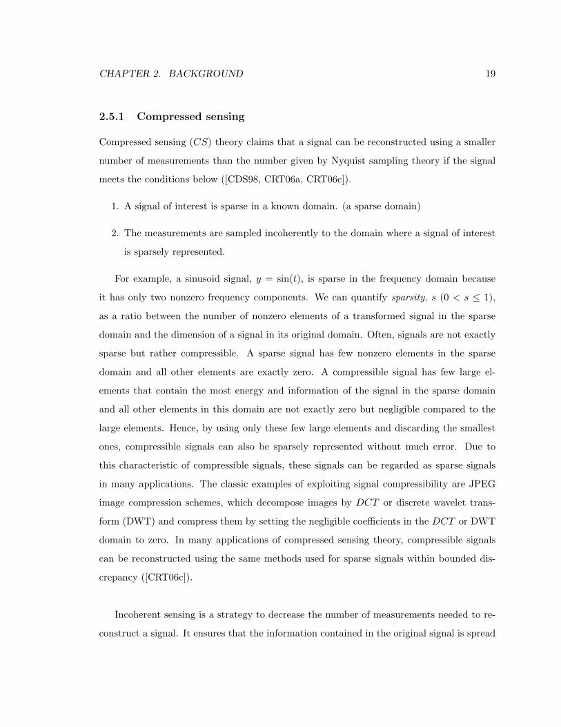
2.5.1 Compressed sensing
Compressed sensing (CS) theory claims that a signal can be reconstructed using a smaller
number of measurements than the number given by Nyquist sampling theory if the signal
meets the conditions below ([CDS98, CRT06a, CRT06c]).
1. A signal of interest is sparse in a known domain. (a sparse domain)
2. The measurements are sampled incoherently to the domain where a signal of interest
is sparsely represented.
For example, a sinusoid signal, y = sin(t), is sparse in the frequency domain because
it has only two nonzero frequency components. We can quantify sparsity, s (0 < s ≤ 1),
as a ratio between the number of nonzero elements of a transformed signal in the sparse
domain and the dimension of a signal in its original domain. Often, signals are not exactly
sparse but rather compressible. A sparse signal has few nonzero elements in the sparse
domain and all other elements are exactly zero. A compressible signal has few large el-
ements that contain the most energy and information of the signal in the sparse domain
and all other elements in this domain are not exactly zero but negligible compared to the
large elements. Hence, by using only these few large elements and discarding the smallest
ones, compressible signals can also be sparsely represented without much error. Due to
this characteristic of compressible signals, these signals can be regarded as sparse signals
in many applications. The classic examples of exploiting signal compressibility are JPEG
image compression schemes, which decompose images by DCT or discrete wavelet trans-
form (DWT) and compress them by setting the negligible coefficients in the DCT or DWT
domain to zero. In many applications of compressed sensing theory, compressible signals
can be reconstructed using the same methods used for sparse signals within bounded dis-
crepancy ([CRT06c]).
Incoherent sensing is a strategy to decrease the number of measurements needed to re-
construct a signal. It ensures that the information contained in the original signal is spread

CHAPTER 2. BACKGROUND 20
out over a set of incoherent measurement functions that are not correlated to each other
and have small correlation with unit vectors in the domain where a signal of interest is
sparse. For example, one of the most commonly used incoherent functions are a set of ran-
domly selected rows of discrete Fourier transform (DFT) matrix. Every DFT coefficient is
a linear combination of all signal elements in its original domain, thus, carries information
of all signal elements. According to CS theory, if a signal is sparse in the DFT domain, by
randomly measuring small number of samples of the signal in the original domain, we can
fully reconstruct the original signal with high probability because these random measure-
ments carry fraction of all signal elements [CRT06a]. If a signal is compressible in the DFT
domain, it still can recover the dominant components of the signal in the sparse domain
but not the negligible ones.
If a signal of interest is sparse in a known domain and its measurements are incoherent,
a sparse signal x0 ∈ Rn can be reconstructed by solving the convex optimization problem
below:
minx
||Ux||1 s.t. ||Ax− b||2 < � (2.12)
Here U ∈ Cn×n is a sparsifying transform and A ∈ Cm×n is a sensing matrix (m < n) where
m is the number of measurements. b ∈ Cm is the measurement of x0 using A (b = Ax0 if
there is no measurement noise) and � is the upper bound on the amount of noise present
in the measurement b.1 If the measurement is not corrupted by noise, � can be set to 0
and the solution of this optimization problem is the exact reconstruction of x0 if we have a
sufficient number of measurements [CRT06a].
2.5.2 Low rank matrix approximation
In the current image processing and computer vision problems, often we are interested in
learning an underlying structure that is common among the images while extracting the
discrepancies between the images. For example, when recognizing faces, it is very often
1If U is an identity matrix, A has to satisfy the incoherent sensing properties. Otherwise AU−1 has tobe an incoherent sensing matrix.

CHAPTER 2. BACKGROUND 21
that a face of the same person does not appear the same in different images due to dif-
ferent color balancing and illuminations in addition to other cosmetic changes. Therefore,
a robust face recognizer learns the underlying structure from a set of training images and
try to recognize the same person from test images[BJ03, WYG+09]. One way to effectively
learn the underlying common structure from a set of different observations is to find the
low rank approximation of a matrix whose columns are vectorized observations. This low
rank approach is more general than face recognition and appears frequently in many differ-
ent applications such as removing occlusion and restoring low-rank texture[ZGLM12], and
detecting anomalies in video surveillances[CLMW11].
The problem of finding a matrix with minimum rank can be formulated as:
minX
rank(X) s.t. ||A(X)−B||2 < �, (2.13)
where X is the row rank structure of the signals that measures to be B when applied to a
function A up to a noise limit �. If the measurement constraint is a convex set, it is well
documented that this problem can efficiently be solved using a nuclear norm heuristic for a
rank metric and convex programming [FHB01]. A nuclear norm of a matrix X ∈ Rm×n is
defined as
||X||∗ =min{m,n}�
i=1
σi(X), (2.14)
where σi(X) are the singular values of X.
Chapter 3
Digital In-painting via l1 Norm
Minimization
3.1 Introduction
The low SNR and the limited angle tomography make analyzing tomograms a challeng-
ing task. Researchers have been trying to manage these problems in various ways. One
way to overcome the low SNR is utilizing colloidal gold beads as fiducial markers to align
tomographic projections precisely. Researchers have also been actively looking for geneti-
cally modifiable labels, equivalent to green fluorescent protein in the light microscopy, that
can help detect specific proteins or macromolecules in noisy tomograms [DFG+09, MD07,
WML11]. The benefits of using markers and labels1 are clear, but there are also disad-
vantages to using them, especially when markers are larger than objects of interest and
significantly denser than the background. A common problem that results from the pres-
ence of colloidal gold beads throughout the sample is the occlusion of features or regions of
interest in projections. Another, perhaps more serious problem, is that 3D reconstruction
algorithms are unable to perfectly handle the large and abrupt contrast difference between
1In this chapter, markers and labels are used interchangeably because they create artifacts of the samenature. However, they have different roles in image analysis. Typically markers are used as landmarks foraccurate alignment and labels are targeted to certain macromolecules of interest for better localization.
22

CHAPTER 3. DIGITAL IN-PAINTING VIA L1 NORM MINIMIZATION 23
a sample and fiducial markers. As a result, a halo or a shadow created by markers is elon-
gated by missing wedge effects, and projects onto neighboring (and not occluded) sample
features. In addition, very serious ripple effects are also very common, in particular when
clusters of markers are imaged only through part of the angular range. Finally it is some-
times impossible not to have markers around objects if they are used as labels.
There are numerous cases where markers themselves or their artifacts interfere with
detecting objects of interest or analyzing them. For example, in CET reconstructions of
intact bacteria, the goal of the image analysis can be to segment filaments through the
length of the cell, or to understand the coherence range of repetitive structures. These
tasks are not possible in the presence of dense artifacts that distort the shape of filaments
or the repeating structures. Also, in CET sub-volumetric averaging of macromolecules and
viruses, the ripples and halos caused by nearby fiducial markers, together with the distor-
tions created by the missing wedge, hinder the precise alignment. When macromolecules
are nanogold-labeled, these electron-dense labels themselves can bias aligning the molecules
as well. Finally, in CET of aqueous suspensions of inorganic nanoparticles, quantitative
analysis of reconstructed volumes can also be biased by fiducial markers. These phenom-
ena are especially pronounced when specimens are thin and markers lie very close to the
target objects, or when markers lump together. Without these artifacts, the specimen of
interest can be studied with greater clarity, and valuable data sets that may include unique
structures or conformations that are short-lived and difficult to capture can be saved from
the shadowing artifacts. Therefore, to utilize the high SNR markers and labels for ana-
lyzing CET reconstructions without side effects, it is necessary to come up with ways to
reduce artifacts created by dense markers, or to erase markers during the image analysis
(skeletonization, segmentation, sub-volumetric alignment, quantitative image analysis of
nanoparticles suspensions, etc).
In this chapter, we propose a new algorithm that removes high contrast objects by
digital inpainting (defined in Sec. 3.2), which utilizes the fact that CET projections can

CHAPTER 3. DIGITAL IN-PAINTING VIA L1 NORM MINIMIZATION 24
be decomposed into a sparse representation in the DCT domain. We fill in the missing
regions occluded by high contrast objects in projections and demonstrate that the resulting
inpainted projections and the reconstructed volume show minimal artifacts around the
regions near high contrast objects. To help readers solidly understand our new algorithm,
we start by reviewing the existing digital inpainting methods and the CS theory which
underlies some of them. Then we show that CET projections are sparse in the DCT
domain and how we can exploit this information to inpaint occluded regions in projections
in the framework of CS. For evaluation, we first examine the inpainted projections and
tomograms of the surface-layer (S-layer) of Bacillus sphaericus, which has a natural short-
range order property that results in projections with a sparse power spectral density. After
confirming the success of our proposed method with S-layers, we move on to inpaint whole
cell data sets of Caulobacter crescentus, which are not naturally sparse but compressible
(defined in Sec. 2.5.1). In each experiment, we compare the perceptual quality of inpainted
projections and reconstructions produced by our algorithm to those produced by the existing
inpainting methods. To assist the perceptual comparison of different inpainting techniques,
we also compute image similarity metrics for the inpainted tomograms. To verify whether
inpainting can also help quantitative analysis of tomograms by removing fiducial marker
artifacts, we average the S-layer units located near the inpainted regions and compare
these averaged volumes to a reference S-layer structure. These qualitative and quantitative
evaluations show that our algorithm can reduce artifacts from high contrast objects and
reveal their neighboring regions more clearly than the conventional algorithms without
creating secondary inpainting artifacts.
3.2 Theoretical background and previous work
High contrast metal artifacts are not a new problem in tomography and there are solu-
tions developed for different imaging modalities that suffer from the same problem. In
the X-ray tomography community, many researchers have been looking for solutions for
this problem, known as metal artifact reduction(MAR) ([WSOV96, ZRW+00, DND+00,

CHAPTER 3. DIGITAL IN-PAINTING VIA L1 NORM MINIMIZATION 25
XRY+05, WK04]) because metal prostheses in patients’ body create artifacts that hinder
accurate medical diagnosis. The most common strategy is to fill in the regions occluded by
metal objects with locally interpolated values or maximum likelihood estimates in projec-
tions. Recently, approaches that specifically formulate MAR in a constrained optimization
framework have been introduced as well ([GZY+06, ZWX10]). They often minimize the
total variation of the reconstruction because typical X-ray images are well approximated
as piecewise constant functions. Metal objects can also be removed in a reconstruction
domain. This approach is less popular because it requires tracing all the artifacts that are
created in the process of reconstruction.
While it appears that these algorithms developed in the X-ray tomography community
can be easily applied to remove high contrast artifacts created by electron-dense markers in
CET , differences in image characteristics make this task challenging. X-ray projections and
tomograms have a higher SNR than CET ones, and X-ray tomograms do not suffer from a
missing wedge problem. In addition to these differences in image quality, X-ray tomograms
have different image statistics due to different contrast mechanisms. As previously men-
tioned, they often contain piecewise constant features while CET tomograms have more
textural ones. Therefore, we need to tailor these methods to remove high contrast objects
for CET .
Researchers in the CET community have also been removing fiducial markers by fill-
ing gaps with locally interpolated pixel values or with random numbers drawn from local
statistics. Although these methods rely on local statistics, boundaries are usually visible
and corrected regions look artificial both in projections and reconstructed volume. This is
because these methods rely on a very simple image model that does not account for the
overall signal property of a projection.

CHAPTER 3. DIGITAL IN-PAINTING VIA L1 NORM MINIMIZATION 26
3.2.1 Digital Inpainting
Digital inpainting is a technique to fill in missing regions in images without visible traces
([BBC+01]). It is basically an interpolation scheme in which image models play an im-
portant role ([CKS02]). Images can be decomposed into two components, structure and
texture, and different image models are applied for these components because they exhibit
different statistical and perceptual characteristics. The first component, structure (also
known as cartoon), is defined as piecewise constant regions of images that also contain
sharp edges. The most common method to inpaint the structural part is a variational
approach, which tries to propagate information from existing parts of an image to missing
regions as smoothly as possible. This approach assumes that an image is a function that lies
in the Bounded Variational (BV) space; one way to implement this approach is to pose it
as a Total Variation (TV) minimization problem ([CS01]). The second component, texture,
is defined as rapidly varying or oscillating regions of images in terms of intensity. Texture
inpainting is often carried out by texture synthesis techniques that analyze the local statis-
tics of observed regions and predict missing ones. Structures and textures can overlay, and
there are approaches which try to inpaint both parts simultaneously ([BVSO03, ESQD05]).
Elad et al. in ([ESQD05]) showed how to use the compressed sensing technique to
digitally inpaint natural images. In this section, we show that CET projections satisfy the
conditions on signals that can be inpainted using the compressed sensing framework.
3.2.2 Sparsity of CET projections
In order to apply the compressed sensing framework to inpaint CET projections, we first
need to find a domain where projections have sparse representations. In general, it is very
difficult to analytically prove that projections of a specimen are sparse or compressible in
any known domain without any prior knowledge of an atomic structure of a specimen. How-
ever, the sparsity or compressibility of arbitrary signals can be demonstrated empirically

CHAPTER 3. DIGITAL IN-PAINTING VIA L1 NORM MINIMIZATION 27
[LDP07, PL09]. For example, there have been extensive studies on the statistics of natu-
ral images and it has been generally accepted that natural images are compressible in the
DCT or DWT domain [TM02]. Following this practice, DCT has been used for sparsifying
textural parts and DWT for structural parts of natural images in [ESQD05]. This section
shows that CET projections are sparse in the DCT domain by evaluating the fidelity of
reconstructions of CET projections using only 1% and 5 % of their largest DCT coefficients
in terms of magnitude. We visually inspect the fidelity of compressed reconstructions and
also quantify the loss in signal energy from compression. We choose DCT as a sparsifying
transform because it sparsifies textural parts of images well, and CET projections contain
large texture parts due to the dense nature of biological specimens. DWT can be another
option. However, DWT is mostly used to sparsify piecewise smooth images ([SED05]), and
the resulting inpainted regions also tend to be flat and texture-less. Therefore, we focused
on DCT in this chapter to preserve the continuity in the image statistics in the inpainting
regions and the neighboring regions.
We surveyed the sparsity of 2D CET projections of B. sphaericus S-layers and of C.
crescentus of various shapes in the 2D-DCT domain using 704 projections from 11 tomo-
grams and 1527 projections from 13 tomograms respectively. Their projection angles vary
between −65◦ and 65◦. We evaluated the closeness between the compressed reconstruction
and the original image using normalized mean squared error (NMSE), which is defined as
||x0−xαDCT ||2F||x0||2F
. x0 is an original image, xαDCT is its compressed reconstruction using DCT
transform at compression rate at α and || · ||F is a Frobenious norm. This metric measures
the portion of signal energy lost from compression. When projections are compressed at
95%, it means that they are reconstructed by using only top 5% of 2D-DCT coefficients
in magnitude. The median loss of energy by compressing projections of S-layers at the
compression rate of 95% and 99% are 0.0011 and 0.0030 respectively. (See Fig. 3.1 plot (a)
and (b).) For the whole cells, the median NMSE is 0.0030 when compressed at 95% and
0.0051 when compressed at 99%. (See Fig. 3.1. plot (c) and (d).) This is very little loss
in signal energy given the high compression rate of 95 % and 99 %. Notice that we can

CHAPTER 3. DIGITAL IN-PAINTING VIA L1 NORM MINIMIZATION 28
also indirectly see that the projections of whole cells are not as sparse as the projections of
S-layers by comparing the loss of energy from compression.
Upper 5% reconstruction(a)
Upper 1% reconstruction(b)
RMSE
(c)
RMSE
(d)
RMSE RMSE
Slayer
NumberofProjections
WholeCell
NumberofProjections
Figure 3.1: Survey of energy loss in compressed 2D-DCT reconstructions of tomo-graphic projections.: In (a) and (b) B. sphaericus S-layers ; In (c) and (d) C. crescentuswhole cells : In (a) and (c), NMSE of reconstructions using only top 5% magnitude2D-DCT coefficients. In (b) and (d) using top 1% coefficients.
When we visually compare the compressed reconstructions with the original projections,
it is very difficult to differentiate the reconstructions from the originals with naked eye. (See.
Fig. 3.2.) In addition to little signal energy loss and high visual fidelity, the statistics of the
residuals, differences between the original image and the reconstructed image, closely follow
the Gaussian statistics, shown in the last column of Fig. 3.2, which implies that the infor-
mation embedded in the discarded coefficients is mostly corrupted by noise.2 From these
2The noise of CET projections have Poisson statistics which can be safely approximated as a additiveGaussian noise when the mean value is sufficiently large.

CHAPTER 3. DIGITAL IN-PAINTING VIA L1 NORM MINIMIZATION 29
observations, we can conclude that projections of B. sphaericus S-layers and C. crescentus
are compressible in the DCT domain.
3.2.3 Incoherent sensing of CET projections
In addition to the sparsity of projections, we also need to prove that the domain where
a signal is measured is incoherent to the domain where the signal is sparse to justify ap-
plying compressed sensing theory for inpainting CET projections. According to [CRT06a],
randomly selected orthonormal basis functions form an incoherent sensing matrix. In our
application, the overall sensing matrix is AU−1, where A, is an identity matrix with missing
rows at the locations where pixels are randomly missing (because gold beads are randomly
located.) and U is a 2D-DCT matrix, which is orthonormal. Therefore our sensing matrix,
AU−1, satisfies the incoherent sensing condition. In addition, we are inpainting small re-
gions of CET projections, our CS-based digital inpainting algorithm satisfies the minimum
measurement constraint for faithful reconstruction.
3.3 Proposed algorithm: Digital inpainting via compressed
sensing
The inpainting procedure starts with identifying objects to be removed. In this chapter,
we choose colloidal fiducial markers (diameter ∼ 10nm) as target high contrast objects to
be removed.3 We find fiducial markers in all projections to avoid creating inconsistencies
between projections. To do this, we select fiducial markers in the projection taken at 0
degree tilt angle and track them through out the tilt series using imodfindbeads and track
functions in IMOD ([KMM96]). When IMOD fails to detect or track the markers to be
removed, we hand-label markers. Based on locations and a radius of fiducial markers, we
create a binary mask for each projection that discards pixels occluded by fiducial markers.
3This algorithm can inpaint any missing or corrupted regions in CET projections, such as X-ray damagedpixels, as long as the problem satisfies the compressed sensing constraints mentioned in Sec. 2.5.1.

CHAPTER 3. DIGITAL IN-PAINTING VIA L1 NORM MINIMIZATION 30
Figure 3.2: B. sphaericus S-layers (1) and C. crescentus (2-3) projections and theirDCT -compressed 2D-reconstructions: (a) Original projections at tilt angle 0 degree. (b-c) Compressed 2D-reconstructions of projection of (a) using only 5% and 1% of the largestDCT coefficients. (d) Normal probability plot of residuals of 5%, 1% reconstructions. Inthis plot, the residuals are plotted against the theoretical normal distribution to assessthe normality of the residuals. If the line is straight, the residuals follow the normalstatistics.

CHAPTER 3. DIGITAL IN-PAINTING VIA L1 NORM MINIMIZATION 31
Once the fiducial markers are all detected and masks are created, we can inpaint the
projections by solving the optimization problem in Eq. 2.12. Here x ∈ Rn is a vectorized
square image where n = N2 and it is the inpainted image when this problem is successfully
solved. N is the number of rows or columns of a square image. We define U ∈ Rn×n as a re-
arranged 2D-DCT matrix that carries out 2D-DCT on a vectorized image x. A ∈ {0, 1}n×n
is a diagonal matrix whose diagonal elements are binary. If the ith element of x is to be
inpainted, A(i, i) = 0 and A(i, i) = 1 otherwise. y ∈ Rm is a vector of observed pixel
values that are not occluded in the original image. � is an upper-bound on the amount of
discrepancy in unoccluded pixels while inpainting occluded ones. To preserve unoccluded
regions as intact as possible, we choose a small value of � from a range of [0.00001, 0.0005]
% of the l2 norm of the original image. By setting � as the noise floor in measurements,
we can also denoise projections ([CDS98]). However, we chose a very small � which is well
below the noise floor not to denoise projections because tomograms are often averaged to
reveal finer details that are often buried in noise.
Large scale convex optimization problems with a non-differentiable objective can take
long time to solve and the optimization problem formulated in Eq. 2.12 certainly belongs
to this category. Therefore, we use a l1 norm minimization solver, NESTA (a shorthand
for Nesterovs algorithm), which is specially developed for solving large scale compressed
sensing problems ([BBC11]). This solver minimizes a smoothened version of l1 norm by
a first-order method. This technique provides a good trade-off between computational ef-
ficiency and numerical accuracy. NESTA is also easy to configure because its parameters
can be intuitively determined. In addition to the sparsifying transform and sensing matrix
in Eq. 2.12, it requires a user to specify only two additional parameters. One is the final
smoothing factor, which determines the accuracy of the solution and the other is the error
bound, � in Eq. 2.12. In our case, the error bound is set to be small to avoid denoising and
the final smoothing parameter is set to be 10−5 to obtain accurate solutions. According
to our experience, if the final smoothing factor is small enough, smaller than 10−3, the
CHAPTER 3. DIGITAL IN-PAINTING VIA L1 NORM MINIMIZATION 32
inpainted regions do not differ much perceptually while a smaller smoothing factor does
provide a solution with smaller l1 norm in the DCT domain. The computational time
increases as the smoothing factor decreases but the increase was in the order of tens of sec-
onds to solve a 2048 × 2048 matrix. NESTA has other parameters that have default values
and according to our experience, these default values provide accurate solutions within a
reasonable amount of time. Therefore, we have not fine-tuned these parameters.
Given these parameters, our inpainting algorithm takes about 5 minutes to inpaint an
image with 2048 × 2048 pixels using NESTA on a PC with Intel(R) Core(TM)2 Duo CPU
E7500 2.93GHz and 8 GB RAM. The whole algorithm including the solver, NESTA, is
implemented in Matlab(TM), and we used an optimized 2D-DCT , not the default one
provided in Matlab, to minimize the run time. Projecting on to and recovering from the
sparse signal domain is the most expensive part of the digital inpainting computation,
totaling about 55% of the runtime. This rather long processing time (compared to seconds
using IMOD) is the price for more sophisticated inpainting. Inpainting a set of images can
be naturally parallelized for each image because each inpainting task is independent of each
other. Therefore, the runtime for inpainting a whole stack of tomographic projections can
be kept constant around the time to inpaint a single image.
3.4 Materials
Two kinds of datasets are used to test CS-based digital inpainting for CET projections:
an in-vitro, ordered self-assembled macromolecular system, and intact bacteria. For the
former, one tomogram of wild type S-layer protein from B. sphaericus (wtSbpA) and two
tomograms of in-vitro recombinant (truncated sequence) S-layer protein (rSbpA) were used
for digital inpainting. 8 additional tomograms of in-vitro recombinant rSbpA (total of 11
tomograms) were used to survey the sparsity of S-layer projections. The intact bacteria con-
sist of three tomograms of C. crescentus intact cells were used for inpainting and additional
10 tomograms of C. crescentus (total of 13 tomograms) were used to survey the sparsity

CHAPTER 3. DIGITAL IN-PAINTING VIA L1 NORM MINIMIZATION 33
of CET projections of intact bacteria. Cell cultures, cryo-grids preparation, cryo-EM data
acquisition and processing were done as previously described in [ACN+10, BCG+10]. B.
sphaericus sample preparation and data acquisition were also done using the identical meth-
ods described in [ACN+10, BCG+10].
All the fiducial alignments were done with RAPTOR ([AMC+08]) and the reconstruc-
tions were performed with the weighted-back-projection provided by IMOD ([KMM96]).
3.5 Results and discussions
In this section, we present inpainted projections and tomograms of isolated S-layers of B.
sphaericus and whole cells of C. crescentus using the proposed method and compare these
images with the results obtained using the existing methods in the CET community. To
the best of our knowledge, there have not been many inpainting algorithms introduced in
the CET community and the most commonly used ones are polynomial interpolation in-
painting implemented in IMOD and random noise inpainting. To evaluate the quality of
inpainting performed by our method, we also inpainted all data sets using IMOD (ccderaser
function) with polynomial orders 0,1,2,4 and Poisson random noise inpainting, which fills
missing regions with randomly drawn pixel values from an estimated Poisson distribution
based on the local statistics.5
First, we visually evaluate the inpainting performance of all inpainting algorithms men-
tioned above by comparing the original projections and tomograms with their inpainted
pairs. Comparing reconstructed volume is very important because inpainting should not
create any secondary artifacts while removing high contrast objects. Secondly, we examine
whether inpainting high contrast objects can actually reveal the structure shadowed by ar-
tifacts by introducing artificial markers and inpainting them. Lastly, we perform a small
4For each data set, the best performing polynomial order is selected for figures in this section.5This method is to replace marker regions with artificially created backgrounds that has the same statis-
tical property of the background noise in CET projections.

CHAPTER 3. DIGITAL IN-PAINTING VIA L1 NORM MINIMIZATION 34
scale S-layer subtomogram averaging experiment to see whether digital inpainting actually
enhances signals of interest in the uncovered regions, and to verify that these part of tomo-
grams can produce meaningful quantitative analysis. The result shows that the projections
inpainted by the proposed method are visually more natural and the corresponding regions
in tomograms show less severe artifacts. There are a few cases where we can see halos of
fiducial markers in reconstructions; however, in those cases, our method still creates less se-
vere artifacts than the existing methods. In addition, artificial fiducial marker experiments
and subtomogram averaging experiments confirm that digital inpainting enhances signals
of interest shadowed by high contrast artifacts by removing them, and both visual and
statistical fidelity of CS-inpainted volume is superior to the ones produced by the existing
methods.
3.5.1 Surface layers
S-layers of B. sphaericus are naturally formed 2D paracrystals that have a sparse structure
in the frequency domain, and their CET projections are also sparse in the DCT domain.
Therefore, our method should be able to inpaint the occluded regions with minimal artifacts.
We confirm that this hypothesis is true by visually inspecting the inpainted projections in
Fig. 3.3. The proposed method inpaints the areas occluded by fiducial markers without
artificial boundaries and the overall regions seem very natural while other methods simply
replace fiducial markers with artificial disks. This difference stems from the unrealistic
image models that the other methods are based upon. The IMOD model assumes that CET
projections locally form polynomials and random noise inpainting assumes that pixel values
within a close range in CET projections are drawn from an I.I.D. Poisson distribution. On
the other hand, our CS-based inpainting method does not create obvious discontinuities in
projections because it assumes that CET projections consist of a few DCT basis functions
which are continuous within the support of images.

CHAPTER 3. DIGITAL IN-PAINTING VIA L1 NORM MINIMIZATION 35
Figure 3.3: CET projections of isolated wild type B. sphaericus S-layer: (a) Beforeinpainting: Fiducial markers are occluding S-layer surfaces. (b) CS inpainting: Markersare removed and no artificial boundaries are visible. (c) IMOD inpainting: Polynomialorder 0 is used, and the markers are replaced by a constant value disk. (d) Random noiseinpainting: The markers are replaced by I.I.D. Poisson random variables, which do notpreserve the continuity of the local pixel values.

CHAPTER 3. DIGITAL IN-PAINTING VIA L1 NORM MINIMIZATION 36
Because our algorithm can inpaint CET projections without visible boundaries and ar-
tificial traces, we also expect that 3D tomograms reconstructed from projections inpainted
by our method will have less severe artifacts than those produced from projections inpainted
by the conventional methods. However, the apparent differences among the inpainted re-
gions of 3D tomograms produced by these different algorithms are not as striking as the
differences among the corresponding areas of the inpainted projections. We can see that
all methods remove markers without many visible traces of inpainting in the reconstructed
S-layers in Fig. 3.4. Although all inpainted reconstructions appear very similar to each
other, those inpainted by IMOD and random noise show more visible boundaries than the
tomogram inpainted by the proposed method. This phenomenon is more clearly visible in
Fig. 3.5 Slayer 1 plots, where we only have two fiducial markers that occlude the surface
of the S-layer. In Fig. 3.5, plot Slayer 1 (b), our method seamlessly unveils the underlying
S-layer unit without any artifacts while the other methods create obvious traces of inpaint-
ing. However, when there are many gold beads that are lumped together and occluding a
large area, all methods are rather unsuccessful at recovering the underlying structure. In
Fig. 3.5, in the second row, the surface of the S-layer is not exactly recovered by any of the
inpainting methods, instead they appear to shrink the area affected by the high contrast
artifacts. This different inpainting between the small and the large inpainted regions seen in
Fig. 3.5 can be attributed to the paracrystalline nature of S-layers. Unit cells of paracrys-
tals preserve their regularity only locally not globally. Therefore, if the occluded region is
small, our method can recover the regular structure in the occluded region without much
difficulty. If the occluded region is large, the unit cells around the occluded region do not
carry enough information to recover the missing structure because the regularity of these
unit cells are not preserved for a long range. Although any of the methods cannot suppress
the obvious inpainting artifacts when the inpainted area is large, the characteristic S-layer
lattice is more clearly visible and the boundaries of the recovered region look more seamless
in the tomogram inpainted by the proposed method than in the tomograms inpainted by
the other methods.

CHAPTER 3. DIGITAL IN-PAINTING VIA L1 NORM MINIMIZATION 37
Figure 3.4: CET reconstructions (tomogram slices) of isolated wild type B. sphaericusS-layer: (a) Before inpainting: The high-contrast artifacts created by colloidal fiducialmarkers are occluding surrounding regions. (b) CS inpainting: Most of the markers andtheir artifacts are removed. The structure of the S-layer around and inside the inpaint-ing regions seems to be better recovered than in the other inpainted reconstructions in(c) and (d). No obvious discontinuities are visible around the inpainting regions. (c)IMOD inpainting: Polynomial order 0 inpainting. Some inpainted areas look artificiallymonotone and smoothened. (d) Random noise inpainting: No artificially smoothenedareas are visible but the structure of the S-layer around and inside the inpainted regionsdoes not seem to be well recovered.

CHAPTER 3. DIGITAL IN-PAINTING VIA L1 NORM MINIMIZATION 38
Figure 3.5: CET reconstructions (tomogram slices) of recombinant B. sphaericus S-layer: In the first row, (a) Before inpainting: The high-contrast artifacts created by twocolloidal fiducial markers are occluding surrounding regions. (b) CS inpainting: Themarkers and their artifacts are removed. The structure of the S-layer around and insidethe inpainting regions appears to be better recovered than in the other inpainted re-constructions in (c) and (d). No obvious discontinuities and artifacts are visible aroundthe inpainting regions. (c) IMOD inpainting: Polynomial order 0 inpainting. The in-painted areas look artificially smoothened. (d) Random noise inpainting: No artificiallysmoothened areas are visible but the structure of the S-layer around and inside the in-painted regions does not appear to be well recovered. In the second row, (a) Markers arelumped together and occluding a large region. (b) All the markers and their artifacts areremoved. The structure of the S-layer around and inside the inpainting regions appearsto be slightly recovered. No obvious discontinuities are visible around the inpaintingregions. (c) The inpainted areas look artificially monotone and smoothened. (d) Noartificially smoothened areas visible but the structure of the S-layer around and insidethe inpainted regions does not appear to be well recovered.

CHAPTER 3. DIGITAL IN-PAINTING VIA L1 NORM MINIMIZATION 39
3.5.2 Whole cells
The ultrastructure of C. crescentus, our model for bacteria in general, is not sparse in any
known domain. However, we have empirically demonstrated that CET projections of C.
crescentus are compressible in the DCT domain; therefore, we expect that our inpainting
method can remove high contrast objects without creating severe artifacts, as it does with
S-layers. This hypothesis is validated by the seamlessly inpainted projections in Fig. 3.6.
The projections inpainted by our CS-based method appear to be more natural to naked
eye, with less visible artifacts, than the projections created by other methods.
As seen in the previous section on S-layers, well-inpainted projections result in tomo-
grams with less severe artifacts. In Fig. 3.7 and Fig. 3.8. we see markers whose high
contrast artifacts cast shadow on the cell membrane. The challenge here is to inpaint the
occluded regions without disrupting the integrity of the neighboring cell membrane. Since
the membrane creates discontinuities that are not very sparse in the DCT domain, the oc-
cluded membranes are not fully recovered after inpainting in the projections as in Fig. 3.6.
However, we still do not find any artificial boundaries around the inpainted regions in the
CS-inpainted reconstructions in both Fig. 3.7 and Fig. 3.8 because our method inpaints
missing pixel values by estimates that blend well with the surroundings without disconti-
nuities, while other methods simply replace markers with artificial disks. If the markers
occlude the membrane in a small number of projections, the back-projected volume does
recover the membrane from the unoccluded projections. In this case, the contribution from
the inpainted membrane averages out as long as inpainting does not create gross errors.
Therefore, we can see membranes clearly without any artifacts in tomograms as in Fig. 3.7
and Fig. 3.8. If markers are occluding specific regions containing sharp edges in most of
the projections, these edges may not be clearly visible in the reconstructions because our
method does not necessarily recover the edges in the projections.

CHAPTER 3. DIGITAL IN-PAINTING VIA L1 NORM MINIMIZATION 40
Figure 3.6: CET projections of C. crescentus: (a) Before inpainting: Fiducial markersocclude the cell membrane. (b) CS inpainting: Markers are removed and no artificialboundaries are visible. At the projection angle of -30 degree, we see markers that lieon the different plane of the tomogram. These markers were not labeled to be removed.(c) IMOD inpainting: Polynomial order 0 was used, and the markers are replaced by aconstant value disk. (d) Random noise inpainting: The markers are replaced by I.I.D.Poisson random variables which do not preserve the continuity of the local pixel values.
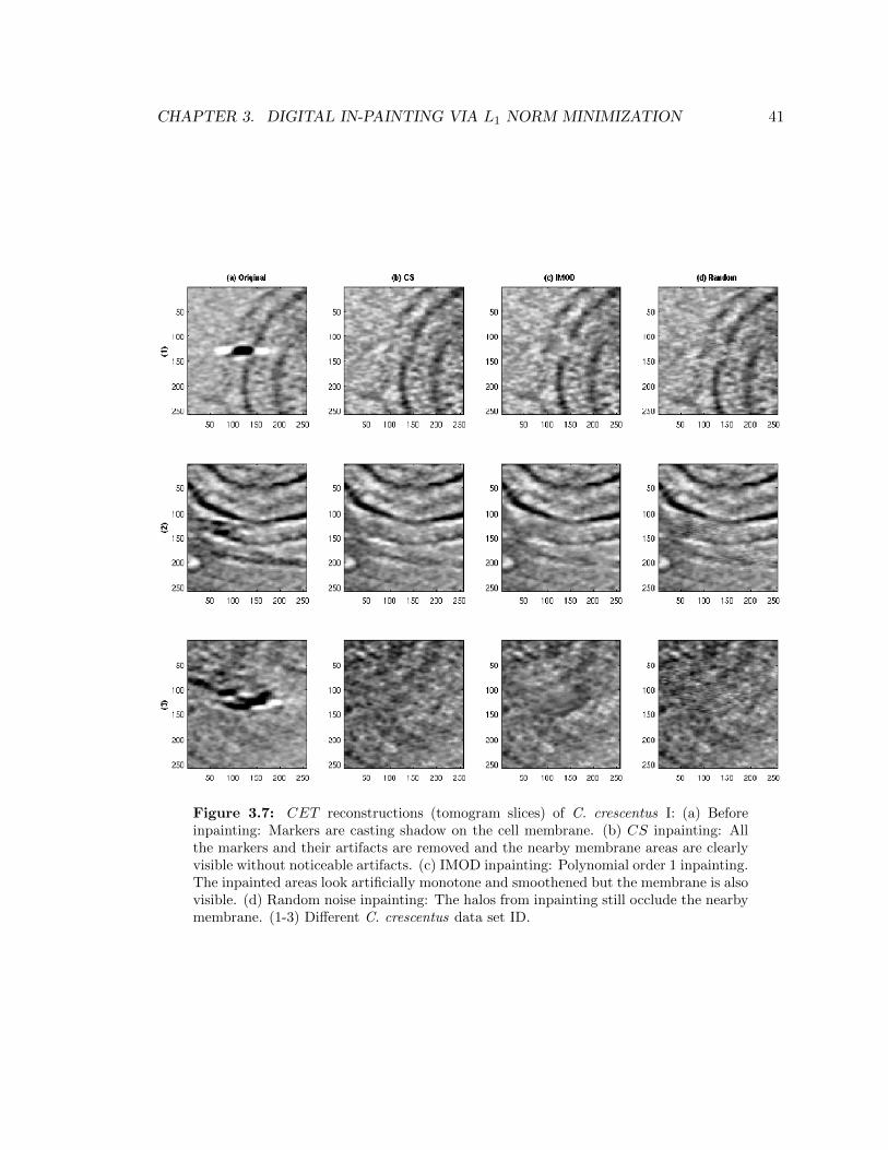
CHAPTER 3. DIGITAL IN-PAINTING VIA L1 NORM MINIMIZATION 41
Figure 3.7: CET reconstructions (tomogram slices) of C. crescentus I: (a) Beforeinpainting: Markers are casting shadow on the cell membrane. (b) CS inpainting: Allthe markers and their artifacts are removed and the nearby membrane areas are clearlyvisible without noticeable artifacts. (c) IMOD inpainting: Polynomial order 1 inpainting.The inpainted areas look artificially monotone and smoothened but the membrane is alsovisible. (d) Random noise inpainting: The halos from inpainting still occlude the nearbymembrane. (1-3) Different C. crescentus data set ID.

CHAPTER 3. DIGITAL IN-PAINTING VIA L1 NORM MINIMIZATION 42
Figure 3.8: CET reconstructions (tomogram slices) of C. crescentus II: (a) Beforeinpainting: Markers are casting shadow on the cell membrane. (b) CS inpainting: Allthe markers and their artifacts are removed and the nearby membrane region is clearlyvisible without noticeable artifacts. (c) IMOD inpainting: Polynomial order 1 inpainting.The inpainted areas look artificially monotone and smoothened but the membrane is alsovisible. (d) Random noise inpainting: The halos from inpainting still occlude the nearbymembrane.

CHAPTER 3. DIGITAL IN-PAINTING VIA L1 NORM MINIMIZATION 43
3.5.3 Artificial fiducial marker experiment
The purpose of inpainting high contrast objects is to reduce the associated artifacts and
reveal the underlying structure of a specimen. To verify whether removing fiducial markers
does uncover the nearby structure, we create artificial fiducial markers on actual CET
projections and remove them by inpainting. We then compare the revealed structure to
the corresponding one in the original tomogram visually as well as using image quality
metrics, NMSE and mutual information (MI). Artificial markers are created in projections
by applying a 2D Gaussian mask at locations calculated according to the single-axis data
acquisition geometry. In Fig. 3.9, we see the 3D reconstructions of the artificial markers
as well as the original tomograms and the inpainted reconstructions. While all inpainting
methods can remove the high contrast artifacts in tomograms, the proposed method creates
less obvious artificial traces from inpainting than others. Also the areas corrupted by
artificial markers appear to be smaller in the CS-inpainted tomograms than in others,
thus revealing the areas that are right next to the fiducial markers. Being able to contain
inpainting artifacts within a small area is especially important when markers are located
very closely to the objects of interest.
The numerical fidelity of the inpainted volumes are also evaluated by two image quality
metrics, NMSE and MI. NMSE measures the discrepancy in each pixel value relative to l2
norm of the original volume, and MI measures the discrepancy in the overall pixel value
distribution between two volumes. According to the information theory, MI quantifies the
amount of information one volume contains about the other ([PMV03]). The larger the MI
between two volumes, the more information of one volume can be explained by using the
information in the other. All metrics are computed using only voxels near the inpainted
regions. The size of a cropped cube-shape volume is 3 times of the diameter of the inpainted
fiducial marker. In Table 3.1, while all inpainting produces a similar amount of pixel-wise
discrepancies according to the median and mean NMSE, the CS-inpainted volumes have
higher MI than other inpainted volumes. This result can be explained by the nature of these
two metrics. While NMSE is blind to the overall composition of volumes, MI compares the
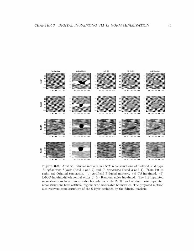
CHAPTER 3. DIGITAL IN-PAINTING VIA L1 NORM MINIMIZATION 44
Figure 3.9: Artificial fiducial markers in CET reconstructions of isolated wild typeB. sphaericus S-layer (bead 1 and 2) and C. crescentus (bead 3 and 4). From left toright, (a) Original tomogram. (b) Artificial Fiducial markers. (c) CS-inpainted. (d)IMOD-inpainted(Polynomial order 0) (e) Random noise inpainted. The CS-inpaintedreconstructions have unnoticeable boundaries while IMOD and random noise inpaintedreconstructions have artificial regions with noticeable boundaries. The proposed methodalso recovers some structure of the S-layer occluded by the fiducial markers.

CHAPTER 3. DIGITAL IN-PAINTING VIA L1 NORM MINIMIZATION 45
NMSE Mutual InformationBead ID CS IMOD Random CS IMOD Random
3DBrdU #1 0.0001 0.0001 0.0002 0.7066 0.5735 0.34403DBrdU #2 0.0001 0.0001 0.0002 0.4035 0.4306 0.27983Dwt1 #1 0.0004 0.0004 0.0004 4.2246 4.1835 4.11113Dwt1 #2 0.0003 0.0004 0.0004 4.1326 3.9970 3.9889Slayer9 #1 0.0003 0.0004 0.0003 1.7839 1.4507 1.7569Slayer9 #2 0.0003 0.0004 0.0003 1.8236 1.4791 1.8002
mean 0.0003 0.0003 0.0003 2.1792 2.0191 2.0468median 0.0003 0.0004 0.0003 1.8038 1.4649 1.7786
Table 3.1: Quantitative comparison of inpainting fidelity using artificial fiducial markersamong different inpainting methods. According to NMSE, all inpainting methods resultin a similar amount of pixel-wise discrepancies on average. However, according to MI,CS-inpainted volumes contain more information that can explain the original volume inmost of the cases.
statistics of pixel values in volumes, and CS-based inpainting does fill in the missing pixel
values using continuous waves that are inferred to preserve the global consistency of each
projection, which also resulted in the consistent tomographic reconstruction.
3.5.4 S-layer subtomogram averaging experiment
One of the advantages of removing fiducial markers is that post processing algorithms such
as subtomogram averaging are less affected by false patterns generated by high contrast
artifacts. To verify this conjecture, we average 77 carefully selected subtomograms of S-
layer units that are right next to fiducial markers from a single tomogram. We choose a
small number of subtomograms for two reasons: 1. We only choose those units near fiducial
markers, and 2. This experiment is intended not to solve a structure of S-layer units but
to see whether inpainted volumes actually contain enhanced signal from the specimen of
interest than the volumes with high contrast artifacts. We repeat the identical averaging
process using the same selection of subtomograms from the original tomogram and the
inpainted tomograms processed by the CS, IMOD and random inpainting methods. The
original tomogram was taken under ∼ −9µm defocus and it has a pixel size of 0.6854 nm.
Each subtomogram has the size of 77 × 77 × 77 pixels (∼ 53nm each side), and they are

CHAPTER 3. DIGITAL IN-PAINTING VIA L1 NORM MINIMIZATION 46
centered on the green spheres shown in the original tomogram (Fig.3.10 plot (a)) and in
the CS-inpainted tomogram (Fig.3.10 plot B). The centers of subtomograms are located
20 voxels (∼ 14nm) away from the fiducial markers. We used the maximum likelihood
method ([SMVC09]) implemented in the Xmipp package for the iterative alignment and
averaging, and the initial reference was chosen by the algorithm. Since we use a single S-
layer reconstruction whose surface is relatively flat without too much shape distortion, we
search only a maximum of 45 degrees around each axis by 10 degree steps for 10 iterations.
In Fig.3.10 plot (b), the subtomograms from the original volume with fiducial markers
failed to align the S-layer structure because of the interfering artifacts created by nearby
fiducial markers. However, when the subtomograms at the same locations from the inpainted
volumes are iteratively aligned and averaged, they can reveal the grid arrangement of S-
layer units. In Fig.3.10 plot (c), We can see that all three averaged subtomograms using
the inpainted volume processed by the CS, IMOD and Random inpainting methods quickly
converged to a meaningful first averaged model or template that could be further refined,
and it is very difficult to tell the differences between these averaged models with naked
eye. Therefore, to achieve more accurate assessment, we compare these averaged models
to an independent averaged S-layer structure derived from different B. sphaericus S-layer
data sets, using Fourier Shell Coefficient criterion. As shown in Fig.3.10 plot (d), we can
see that the averaged S-layer volume from the CS-inpainted tomogram actually has higher
FSC than the ones from the other inpainted volumes especially near the spatial frequency
that corresponds to the periodicity between S-layer units. The periodicity of S-layer unit
is reported to be ∼ 13.5nm, and the diameter of each unit is ∼ 9.375nm. Also, the CS-
inpainted volume can produce an averaged S-layer structure comparable to the one using
the subtomograms from the fiducial marker free regions of the tomogram in terms of FSC.6
We computed FSC using bresolve from Bsoft ([HCWS08]). This result confirms that digital
6We also averaged 77 subtomograms from the fiducial markerless regions in the same tomogram usedfor this experiment described in the paragraph above. Except the location of the subtomograms, all otherexperiment parameters are controlled to be the same as the ones used for averaging subtomograms nearfiducial markers and their inpainted regions.

CHAPTER 3. DIGITAL IN-PAINTING VIA L1 NORM MINIMIZATION 47
Figure 3.10: Comparison of the averaged B. sphaericus S-layer unit models using theoriginal and the inpainted tomograms. : (a) S-layer unit selections( marked by greencircles) in the original volume before inpainting (left) and in the CS-inpainted volume(right): The inset in the left hand side plot contains the fiducial markers that create theartifacts (located 20 voxels above the S-layer). (b) Iso-surfaces of the averaged S-layermodel from the original tomogram (left) and the CS-inpainted one (right): It is obviousthat the alignment procedure cannot align the S-layer lattice in the original tomogramwhile it can produce a fair initial S-layer lattice model from the CS-inpainted tomogram.(c) Averaged S-layer volumes in gray scale volume slices: 1. The original raw volumefailed to converge to a S-layer lattice structure. 2-4. All inpainted volumes convergeto a S-layer lattice structure with subtle differences. However, we can still observe thatthe averaged volume using the CS-inpainted tomogram show clearer barrel shape of aS-layer unit. (d) Quantitative comparison using FSC: Near the periodicity of S-layerunits, spatial frequency = 1/13.5 ∼ 0.0741(1/nm), the averaged S-layer volume from theCS-inpainted volume has the highest FSC which is very close to the averaged S-layervolume using fiducial markerless part of the original volume. The vertical line refers tothe calculated location of the first zero crossing created by the contrast transfer function(CTF) with ∼ −9µm defocus for our microscope.

CHAPTER 3. DIGITAL IN-PAINTING VIA L1 NORM MINIMIZATION 48
inpainting can enhance signals from the structures occluded by removing high contrast
artifacts; in addition, by utilizing the structural information such as the sparsity of CET
projections in the DCT domain, our CS-based inpainting method can actually remove
artifacts more intelligently, which helps to align and refine the underlying structure.
3.6 Conclusions and future work
We have presented a digital inpainting algorithm based on compressed sensing theory, which
effectively removes artifacts created by high contrast objects such as fiducial markers. Our
algorithm estimates missing pixel values that sparsify the inpainted CET projections in
the DCT domain. This technique shows better performance in removing artifacts than the
conventional algorithms because it exploits the sparse or compressible nature of CET pro-
jections in the DCT domain. The proposed method successfully fills missing regions with
minimal distortions or artifacts, such as halos, shadows or ripples, in both projections and
reconstructions. It always provides projections and reconstructions that are perceptually
better than or as desirable as those provided by the conventional methods.
Without these adversary artifacts created by high contrast objects such as fiducial mark-
ers or individual macromolecular tags, specimen areas in the immediate vicinity of these
objects can be studied with greater clarity and the specimen can be used for further analy-
sis. For example, we can crop sub-volumes from these regions and use them for alignment
and averaging. This is very well illustrated in the case of the S-layer shown in Fig. 3.10.
Moreover, if our goal is to compute sub-volume averaging of tagged macromolecules, we can
inpaint their high contrast tags that can bias the alignment of the target macromolecules.

Chapter 4
Subtomogram Averaging via
Nuclear Norm Minimization
4.1 Introduction
To address the low SNR and the missing wedge distortion of cryo-ET reconstructions, one
acquires many sets of projections from multiple copies of the structure of interest and com-
bines them into a single reconstruction: by averaging multiple observations we can reduce
noise and thereby effectively raise the SNR. Moreover, because the specimens in the sample
holder are flash frozen in essentially random orientations, their projection data will have
missing wedges in different locations when aligned to a common orientation. Consequently,
combining sufficiently many observations allows us to fill in the frequency domain and to
eliminate the missing wedge. Although the general idea is simple, this process is by no
means trivial and has itself two main difficulties. The first difficulty is that the orientations
and the centers of each of the macromolecular complexes in the sample are unknown. The
second difficulty, when the sample contains a mixture of heterogeneous structures, is that
the class or type of each macromolecular complex is unknown. The subtomogram averaging
problem thus consists of two sub-problems: alignment and clustering/classification.
49

CHAPTER 4. SUBTOMOGRAMAVERAGING VIA NUCLEAR NORMMINIMIZATION50
In this chapter we propose a new approach for the reference-free alignment and 3D to-
mographic reconstruction from a heterogeneous data set that may be partial in the sense
of the missing wedge. The approach is based on rank minimization and its nuclear-norm
relaxation, and we therefore refer to it as NN-CET (nuclear-norm based cryo-ET). The
inspiration of this algorithm comes from the robust image alignment work by Peng et
al. [PGW+12], in which a set of translated and rotated images with distortions, such as
different lighting conditions and partial occlusion, is aligned by means of iterative lineariza-
tion and nuclear-norm minimization. Our proposed algorithm is novel in several respects.
In particular, it
1. jointly solves the alignment and clustering problem;
2. introduces matrix rank as a collaborative metric to evaluate the alignment and clus-
tering accuracy;
3. estimates the alignment parameters by solving a series of convex optimization prob-
lems; and
4. is reference-free and does not even generate a reference model internally.
While this approach is promising, its current implementation has high computational
requirements and some convergence issues. As a result we were not able to align volumes
larger than 32 × 32 × 32 voxels and it requires coarse pre-alignment before starting our
algorithm.
To understand the context of this approach, we review existing works in Section 4.2 and
then provide a detailed discussion and derivation of the proposed method in Section 4.3. To
examine the effectiveness of the new method we describe experiments on two reconstruction
tasks using synthetic data sets in Section 4.4 and discuss the current algorithm’s limitations.
4.2 Previous Work
In the case of reconstructing a single structure, subtomogram averaging reduces to an
alignment problem, which has been well studied. Optimal alignment parameters are often

CHAPTER 4. SUBTOMOGRAMAVERAGING VIA NUCLEAR NORMMINIMIZATION51
recovered by means of an exhaustive search over a predefined discrete range of parameters
[KFB+13, SMVC09, FMZ+05]. These methods work well for coarse alignment, but can
suffer from high computational complexity for accurate alignment where the search is over
a larger and finer parameter grid. Several approaches based on harmonic analysis have been
proposed to reduce this complexity [CPH+13, XBA12, BSL+08].
Single particle methods can also provide very high resolution density maps of isolated
and purified macromolecules. However, these methods require a reliable reference against
which all electron micrographs are aligned in order to find the correct alignment angles as
well as classes if the sample micrographs contain multiple classes. Since macromolecules are
purified, their structure in their native state cannot be easily resolved using this method.
Often, however, the structures of interest are not homogeneous, especially when they
are in their native state [MS09]. For the high-resolution reconstruction of each structure
it is therefore critical that both classification and alignment be accurate. Unfortunately,
these two problems are intricately linked: without good classification it is hard to find
meaningful alignment parameters; likewise, accurate classification is extremely challenging
without good alignment parameters. Pairwise comparison between subtomograms may seem
to be a solution, but this is compounded by an extremely low SNR and the missing wedge
problem. Various methods have been proposed to overcome these challenges by jointly
or alternatingly solving these subproblems. Indeed, such methods have been successfully
applied to uncover high-resolution macromolecular structures in their native state [BNR+12,
KCW+10, BS09, NSP+06, ZLBJ+06, FMZ+05]. Nevertheless, the subtomogram averaging
problem is far from solved and remains an active area of research.
By far the most widely used method for the subtomogram averaging problem is to solve
the clustering and the alignment problems iteratively by alternating between them (see
for example [KFB+13, BSL+08, SB08, Win07, FMZ+05] among many others). During the
alignment stage, these algorithms try to find the alignment parameters that are optimal
with respect to the current clustering. In most of these algorithms, this is done by means of
class reference models: a set of alignment parameters is determined by minimizing the dis-
similarity between a class reference and a subtomogram. This is complicated by the missing

CHAPTER 4. SUBTOMOGRAMAVERAGING VIA NUCLEAR NORMMINIMIZATION52
frequency information in each subtomogram, and complex similarity metrics that take this
into account have been proposed. Perhaps the most commonly used metric between two
reconstructions with missing wedge is the constrained correlation between the angular com-
ponents that are observed in both reconstructions[CPH+13, XBA12, BSL+08, FMZ+05].
Another metric is proposed by Kuybeda et al. [KFB+13], who use the nuclear norm as a
metric to evaluate the overall alignment.
The reference classes used in alignment are typically determined by one of two ap-
proaches: they can either be calculated internally by averaging randomly selected subtomo-
grams in the data set, or they can be three-dimensional density maps of the target structures
that have been estimated externally. Once subtomograms are aligned to a reference, the
next clustering iteration can start, where all subtomograms are reclustered using well-known
methods such as hierarchical clustering or other methods based on multivariate statistical
analysis [vHF81].
One method that does not alternate between the alignment and clustering is the maximum-
likelihood (ML) approach by Scheres et al. [SMVC09]. This approach explicitly assumes
that tomograms contain heterogeneous structures and incorporates alignment and cluster-
ing into a single likelihood optimization problem. Nevertheless, this approach still relies
on a metric that quantifies the pairwise difference between a reference and an observation.
In addition, like many of the algorithms mentioned above, it also exhaustively searches for
rotation and translation parameters within a user-defined range.
Image alignment and clustering problems are also actively researched in various other
fields [PMV03, ZF03, Bro92]. In the computer vision community, for instance, there is an
increased interest in analyzing uncontrolled images and videos shared by users online. Ana-
lyzing such images shares some of the difficulties encountered in the subtomogram averaging.
First, user-generated images are heterogeneous and not aligned. Second, these images can
exhibit various degrees of missing information due to occlusion or varying lighting con-
ditions. To align and classify these natural images, various robust alignment algorithms
have been introduced [PGW+12, WN12, ClTCB11, lTB03, VGS08]. Many of these algo-
rithms exploit certain inherent low-dimensional structures in the data set, such as sparsity

CHAPTER 4. SUBTOMOGRAMAVERAGING VIA NUCLEAR NORMMINIMIZATION53
or low-rankness. By taking advantage of this, it is possible to robustly align or classify
noisy and corrupted images. These approaches have been successful in recognizing faces in
natural images [PGW+12], analyzing 4D computed tomographic images [GCSZ11], and in
the generation of magnetic resonance images [WN12].
4.3 Methodology
This section shows how a low-rank matrix optimization problem can be used to align,
reconstruct and classify 3D structures. The motivation for the proposed approach and its
derivation is best explained starting from the data generation process.
4.3.1 Formation of the Signal
In cryo-ET we would like to reconstruct the density function of a small number of different
structures. Ideally, we would be able to generate a density function sl : R3 → R for each of
the l = 1, . . . , k different structures. Assuming that the density of the macromolecular struc-
tures in the sample are sufficiently separated from each other and that the tilt-series data
has been appropriately segmented, we can consider the process that generates a tilt-series
for an individual macromolecular structure as following. Suppose that a macromolecular
structure i ∈ [1, N ] belongs to a class ci ∈ [1, k] where N is the number of all observations.
Then we can describe each observation’s density in a normalized coordinate system by ap-
plying a suitable rigid transformation to the coordinate system, consisting of a rotation and
a translation. Denoting this transformation by τθi , with rotation and translation parameters
θi, we obtain the density function
fi = sci ◦ τ−1θi
. (4.1)
This assumes that all macromolecular structures of the same type have the exact same
density. In practice this will not hold exactly, but we can view density function s as an
average density function for the class and model deviations and slight perturbations from
this average as noise.

CHAPTER 4. SUBTOMOGRAMAVERAGING VIA NUCLEAR NORMMINIMIZATION54
With the given macromolecular structure transformed to its physical orientation and
location we can now generate a tilt series. In practice this is done by collecting projection
data with the sample holder tilted at different angles. Here we equivalently fix the macro-
molecular structure and rotate the projection plane around the y axis instead. For a given
rotation angle α the projection function P : R3 → R2 for density function f is given by
Pα(fi)(u, v) =
� T
−Tfi
u cos(α)− γ sin(α)
v
u sin(α) + γ cos(α)
dγ. (4.2)
There are several simplifying assumptions we make here. First, we have chosen some-
what arbitrary integration limits. Mathematically we can choose (−∞,∞), but in practice
we only integrate from the irradiation source to the detector. Second, we assume that the
contrast-transfer function (CTF) is the identity. When a good model for the CTF is known,
however, this would be easy to integrate in (4.2). The second assumption is that there is no
degradation of the macromolecular structure in subsequent projections; i.e., the function fi
remains constant during the acquisition process. The sampling data d(i,j) for macromolec-
ular structure fi is obtained by evaluating Pα at a tilt angle of αj where j ∈ [1,M ], and
applying a suitable noise process. M is the number of projections.
Given only discrete data, the best we can hope for is to reconstruct discretized volumes
xl of the density functions sl. We can transform xl back to a function using for example (tri-
linear) interpolation: sl := I(xl). The resulting function can then be used for projections
by substituting sl in (4.1) by sl, followed by application of (4.2).
4.3.2 Rank Minimization
By reordering the elements we can express each 3D volume as a column vector xi and form
a matrix
X∗ = [x1, x2, . . . , xN ], (4.3)

CHAPTER 4. SUBTOMOGRAMAVERAGING VIA NUCLEAR NORMMINIMIZATION55
where X∗ ∈ Rn×N , with n the number of voxels in each discretized volume xi. If we knew
the transformation parameters θ = {θ1, . . . , θN}, then we would be able to approximately
estimate the measured data, d(i,j), by evaluating the projections of the interpolated data
I(xi) under transformation τ−1θi
at locations (u, v) ∈ G:
d(i,j) ≈�Pαj (I(xi) ◦ τ−1
θi)(u, v)
�(u,v)∈G
,
where d(i,j) ∈ Rm×1, with m is the number of pixels in each projection image. For fixed θi
and αj , and assuming tri-linear interpolation, we can write the projection of the transformed
xi as the matrix vector product A(i,j)xi where
A(i,j) :=�Pαj (I(·) ◦ τ−1
θi)(u, v)
�(u,v)∈G
,
where A(i,j) ∈ Rm×n. From this, it may seem that we can reconstruct xi from data points
d(i,j) by solving (if feasible):
find x such that �A(i,j)x− d(i,j)�2 ≤ σ, ∀j, (4.4)
where j ∈ [1,M ] indexes the tilt angles, and σ is an estimate of the noise/misfit level. This
formulation requires that projections of the reconstructed volume x, match the observed
projection data up to the given noise level. Even though the transformation parameters
are given, this procedure would not give us the desired result. The reason for this is that
the reconstruction of each macromolecular structure i is treated entirely independently and
consequently suffers from the missing wedge problem. Moreover, even if two instances i1
and i2 are from the same class, i.e., ci1 = ci2 , there is absolutely no guarantee that xi1 = xi2 .
This is where low-rank matrix optimization comes in. If we carefully look at (4.3) we
can see that the rank of X∗ is at most equal to the number of distinct columns. In typical
cryo-ET settings the number of distinct classes k is very small compared to the number of
instances N , and much smaller than the length of each vector xi. Taking this into account

CHAPTER 4. SUBTOMOGRAMAVERAGING VIA NUCLEAR NORMMINIMIZATION56
we can modify (4.4) to the problem
minimizeX
rank(X) s.t. �A(i,j)xi − d(i,j)�2 ≤ σ, ∀i, j, (4.5)
where xi is the i-th column of X. Using the rank takes care of two things. First, it
provides the heuristic on how heterogeneous the structures are in the entire sample set,
which can help us decide on the number of classes (more on this below). Second, the rank
structure links columns together, which means that, in effect, all the data for a given class
are combined, thereby solving the missing-wedge problem (provided of course that the data
covers the entire frequency space).
There are two problems with (4.5). The first problem is that it assumes that the
transformation parameters θi are known. This, of course, is a fundamental problem in
subtomogram averaging, where even a rough approximation may be difficult to obtain. The
second problem is that, even if we did know all parameters, rank minimization would still
be an NP-hard problem [MJCD08, RFP10]. We discuss each of these in more detail below.
4.3.3 Nuclear-Norm Approximation
One of the well-known approaches of avoiding the complexity associated with minimizing
the rank is to replace rank(X) by the nuclear-norm �X�∗, which is defined as the sum of the
singular values of X [RFP10]. This convex approximation can be seen as a generalization of
the highly-successful use of �1 instead of the cardinality, often referred to as �0, in compressed
sensing [CRT06b, CT06, Don06] (applied, in this case, to the vector of singular values).
Applied to (4.5) this gives
minimizeX
�X�∗ s.t. �A(i,j)xi − d(i,j)�2 ≤ σ, ∀i, j. (4.6)
As an example of this, we generated four different two-dimensional classes xi of size 33×33
(see Figure 4.1(a)). From this we generated 300 instances that were rotated uniformly at
random, and translated by up to ±10%. A tilt series, consisting of 11 equally-spaced

CHAPTER 4. SUBTOMOGRAMAVERAGING VIA NUCLEAR NORMMINIMIZATION57
projections at angles ranging from −10◦ to +10◦ and sampled at 50 points, was then
generated for each instance. We then solved (4.6) by writing it as a series of penal-
ized formulations and solving them using, a fast iterative shrinkage-thresholding algorithm
(FISTA) [BT09a, BT09b]. The images corresponding to several of the columns xi of the
solution X∗ are illustrated in Figure 4.1(b). Despite the fact that no class information
was given, nuclear-norm minimization is still capable of combining the information from
the various instances of each class and obtaining accurate reconstructions. In other words,
nuclear-norm minimization is able to find a parsimonious model that explains the data.
Without the low-rank structure each reconstruction would simply have constituted a back-
projection from very incomplete data.
(a) (b)
Figure 4.1: Density of (a) four ground-truth structures, and (b) image representationof several columns of the solution X∗ to the nuclear-norm minimization problem whengiven a limited number of projections for each instance, along with their rotation andtranslation parameters, but without any information about the structure classes. Fourdistinct classes matching the ground-truth structures are clearly recovered.
4.3.4 Finding the Transformation Parameters
It now remains to incorporate the transformation parameters into the problem formulation.
For simplicity of notation and to make the dependency on θi explicit, we denote by Aθi ∈RmM×n the linear operator obtained by stacking projection matrix A(i,j) and likewise denote
by di ∈ RmM×1 the stacking of projection d(i,j). We further write θ = {θ1, . . . , θN}. Addingthe transformation parameters to (4.6) and combining the misfit of all data points for a
given xi, we obtain
minimizeX,θ
�X�∗ s.t. �Aθixi − di�2 ≤ σi ∀i, (4.7)

CHAPTER 4. SUBTOMOGRAMAVERAGING VIA NUCLEAR NORMMINIMIZATION58
with misfit parameters σi modified accordingly. Despite its friendly appearance this formu-
lation is still difficult to solve due to the nonlinearity of Aθi . Inspired by the work of Peng
et al. [PGW+12] we apply iterative linearization of A. The idea is that for sufficiently small
changes Δθi and Δxi we can approximate
A(θi+Δθi)(xi +Δxi) ≈ Aθi(xi +Δxi) + Jθi(xi)Δθi,
where Jθi(xi) ∈ RmM×6 denotes the Jacobian of Aθixi with respect to θi; that is, the changes
in the projection with respect to the transformation parameters of the transformed volume
xi. In our application, the observed tomograms are aligned by finding six transformation
parameters corresponding to the rotation and translation along X, Y, and Z axes. Note
that, due to the use of linear interpolation, Aθixi is not differentiable everywhere, although
the set of parameters θi at which this occurs is measure zero. For our experiments we use
finite-difference approximation for the Jacobian, thereby avoiding this problem. Adding
superscript iteration numbers k to the parameters we summarize the iterative algorithm as
follows. At every step we solve:
Xk+1,Δθk := argminX,Δθ
�X�∗ (4.8)
s.t. �Aθki(xi) + Jθki
(xki )Δθi − di�2 ≤ σi, ∀i
and then update θk+1 = θk + βΔθk, with stepsize 0 < β ≤ 1.
4.3.5 Solving the Subproblem
We solve each subproblem (4.8) by first reformulating it as a conic problem and then solving
it using templates for first-order conic solvers (TFOCS) [BCG11]. For the reformulation we
use the Lorentz cone, which is defined as K := {(x, σ) ∈ Rn × R | �x�2 ≤ σ}. With this it

CHAPTER 4. SUBTOMOGRAMAVERAGING VIA NUCLEAR NORMMINIMIZATION59
is easy to see that we can rewrite (4.8) as
minimizeX,Δθ
�X�∗
subject to
Aθki
Jθki(xki )
0 0
xi
Δθi
+
−di
σi
∈ K, ∀i,
which is the final formulation of the subproblem.
4.3.6 Configuring the Solver
The proposed solver requires estimates for the noise level σi as well as the initial rotation
and translation parameters. The noise level needs to be chosen with care; choosing a σ
value that is too large results in the trivial solution X = 0, whereas choosing σi too small
leads to overly restrictive conditions and no feasible solutions. The noise level can either
be based on the experimental setup, or in a more heuristic way by choosing σi equal to
the norm of the projections and then gradually reducing it. Due to the non-convex nature
of the overall problem, the initial alignment parameters cannot deviate too much from the
desired alignment parameters. The suggested procedure therefore requires estimating initial
alignment parameters.
4.4 Experiments
We now evaluate the alignment and clustering performance of our proposed algorithm, NN-
CET, by comparing it against the performance of ML-TOMO [SMVC09], which is one of
several publicly available and widely used subtomogram algorithms in the community. We
used this particular method since it does joint alignment and clustering in a single framework
like our approach. In particular, we used the ML-TOMO implementation included in the
Xmipp Version 2.4 software package [SMVM+04].

CHAPTER 4. SUBTOMOGRAMAVERAGING VIA NUCLEAR NORMMINIMIZATION60
4.4.1 Experiment Setup
Data generation
For test problems we used two sets of 3D density maps of macromolecules that have been
studied by single particle electron microscopy. The first set contains GroEL (EMD-1042)
and GroEL/ES (EMD-1180) [RFR+01]. The second set contains three different conforma-
tions of Helicase molecules (EMD-1135,1146,1148) [NRRM+06]. The density maps for these
structures were downloaded from the Electron Microscopy Data Bank (EMDB) [emd]. For
the experiments, we rescaled the model structures while retaining the relative scales. The
original GroEL molecule in EMDB has a 3D volume of size 128 × 128 × 128 voxels and a
voxel width of 1.74 A, and GroEL/ES has a size of 192 × 192 × 192 voxels and a width
of 1.4 A. The first two Helicase molecules are of size 80 × 80 × 80 voxels, the third one
is of size 64 × 64 × 64 voxels. All Helicase molecules have a voxel width of 4.1 A. Given
the computational complexity of this method, all models were re-sampled using tri-linear
interpolation to a 32× 32× 32 volume of voxels of size 8.2 A in each dimension preserving
their relative size. Example density maps for GroEL and GroEL/ES, as well as Helicases
are illustrated in the top row of Figure 4.2.
To generate each simulation data, we sampled N = 100 instances with classes inde-
pendently chosen at random with uniform probability of 0.5 for each of the classes GroEL
or GroEL/ES. We then rotated the density function of each instance by (φxi , φyi , φ
zi ) ∈
[−180, 180]× [−180, 180]× [−180, 180] degrees at uniformly random and then translated the
rotated volume by (τxi , τyi , τ
zi ) ∈ [−5, 5]× [−5, 5]× [−5, 5] pixels at uniformly random. After
these rigid-body transformations, we applied the Radon transform to each of the instances
at 25 projection angles α = {−60,−55, . . . , 55, 60} degrees. Two-dimensional projections of
size 46×46 pixels1 were generated using the projxyz function in IMOD[KMM96]. The pixel
size in the projection was chosen to match that of the individual voxels and the grid size was
chosen slightly larger than the data volume dimension to ensure that all relevant projection
1The projection size of 46 pixels corresponds to the maximum projection width of a 32× 32× 32 volumewhen rotated along a single axis.

CHAPTER 4. SUBTOMOGRAMAVERAGING VIA NUCLEAR NORMMINIMIZATION61
information was captured. The clean projections were then corrupted using i.i.d. Gaussian
measurement noise to obtain SNR levels of 1, 0.1, 0.03, and 0.01. Our definition of SNR is
var(x)var(n) , where x is the noiseless original projection image which is normalized to have zero
mean and unit variance and n is additive Gaussian noise with zero mean. Examples of the
observed projections of the GroEL and GroEL/ES density maps are shown in Figure 4.2
GroEL GroEL/ES
X Y Z X Y Z
SNR=1 0.1 0.03 0.01
GroEL
GroEL/E
S
Figure 4.2: Top row: Cross sections of the original GroEL and GroEL/ES volumesalong the X, Y , and Z axes. Second and third rows: Radon measurements of GroELand GroEL/ES, respectively, for SNR 1, 0.1, 0.03, and 0.01.
For Helicases we have 3D density maps for each of the three conformation types, cross
sections of which can be seen in Figure 4.3. From these density maps we again generated
a set of N = 100 instances with conformation types chosen uniformly at random. Then
we successively applied the rotation, translation, and projection steps as described for the
GroEL and GroEL/ES dataset, and added measurement noise. Examples of the resulting
observations are shown in Figure 4.4.
Solver Setup and Parameter Initialization
The NN-CET algorithm requires three sets of initial parameters: matrix X, translation
and rotation parameters, and noise level estimates. For the initial X we simply generate
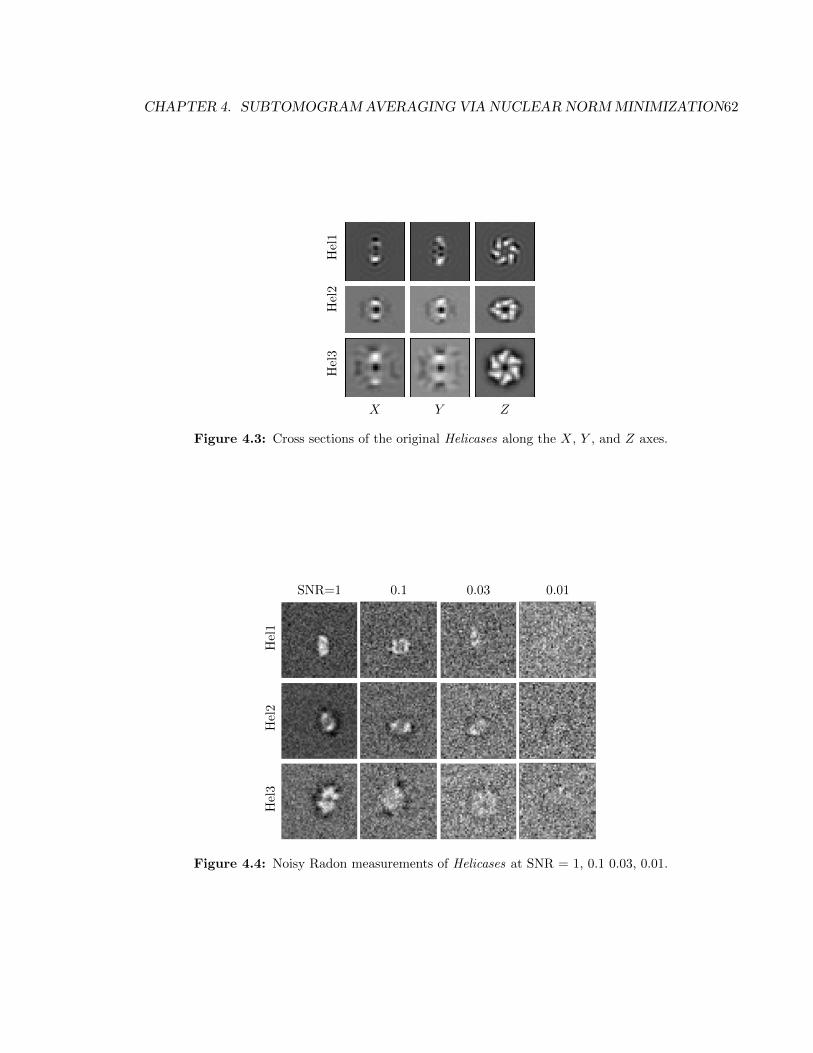
CHAPTER 4. SUBTOMOGRAMAVERAGING VIA NUCLEAR NORMMINIMIZATION62
Hel1
Hel2
Hel3
X Y Z
Figure 4.3: Cross sections of the original Helicases along the X, Y , and Z axes.
SNR=1 0.1 0.03 0.01
Hel1
Hel2
Hel3
Figure 4.4: Noisy Radon measurements of Helicases at SNR = 1, 0.1 0.03, 0.01.

CHAPTER 4. SUBTOMOGRAMAVERAGING VIA NUCLEAR NORMMINIMIZATION63
a random matrix with entries sampled i.i.d from the standard normal distribution N (0, 1).
The initial translation parameters are calculated by finding the center of gravity2 of each to-
mographic reconstruction, and the initial rotation parameters are randomly selected within
a range of [−15, 15] degrees from the correct value.
We have also experimented with running the application without the initial centering,
for situations where mass centering does not provide reliable estimates. In this case the
method does find a reasonable estimate of the centers, but the initial translation errors can
increase errors in the angular estimates. For this situation we use the proposed method
in a two-stage approach. First, the algorithm is run to estimate the center of structures
instead of mass centering. In the second stage we reinitialize and rerun the algorithm
using the calculated translation parameters from the first stage. Both approaches, with
mass centering and with two step processing, produce equivalent alignment and clustering
accuracy.
Finally, we need to provide noise level estimates σi. In our experiments, we used the
actual noise levels in each observation. It is important to have a reasonable value for σi to
obtain high alignment accuracy. When σi is too small there may not be a feasible solution
to (4.8). Likewise, we should certainly choose σi to be smaller than �di�2 otherwise the
corresponding solution xi will be zero.
Similarly for testing ML-TOMO, the initial rotation parameters were set within a range
±15 degrees around the ground truth rotation parameters for both the GroEL & GroEL/ES
and Helicases experiments. ML-TOMO was configured to search over a range of ±30 de-
grees around the initial alignment to allow more freedom in the alignment procedure. The
granularity for the rotation angles was set to be five degrees. The number of references is
set to two for GroEL and GroEL/ES, and three for Helicases. ML-TOMO simulations ran
for 20 iterations. The number of iterations for ML-TOMO is shorter because we observed
that the estimated alignment parameters as well as classes did not change much after about
2The center of mass of each tomogram is calculated by weighted sum of voxel coordinates, where theweight for each voxel is defined as the voxel’s gray level value divided by the sum of gray values of all voxels.For mass centering, a user does not need to provide 3D reconstructions but the algorithm will automaticallyreconstruct 3D volumes given tilt series information and calculate mass centers.

CHAPTER 4. SUBTOMOGRAMAVERAGING VIA NUCLEAR NORMMINIMIZATION64
15 iterations.
Evaluation Metrics
We use two metrics to evaluate the quality of the resulting alignments: 1. Difference in the
recovered and the ground truth alignment parameters. 2. Difference in the recovered density
functions and the ground truth ones. The first metric quantifies the discrepancy between the
recovered alignment parameters and the true alignment parameters. We measure the error
in rotation parameters by comparing the rotation matrices. Given two rotation matrices S
and R in SO(3), we can define their inner-product as the trace of the product: �R,S� =Tr(RTS). Based on this we can derive two quantities. First, the inner product induces a
squared norm �S�2 = �S, S�, where �·� can be verified to be the Frobenius norm. Second, we
can define angles αr(S,R) (in radians) between two rotation matrices by using the standard
definition
cos(αr(R,S)) :=�R,S�
�R�F �S�F.
The Frobenius norm of a rotation matrix in SO(d) is√d, and we therefore define the angles
in degree between two rotations as
α(R,S) :=180
π· acos
�Tr(RTS)
3
�.
Our proposed method recovers rotation and translation parameters without any fixed
reference, which makes measuring the error to the ground truth challenging. As an example,
we can rotate all density maps (or at least those within the same class) arbitrarily without
affecting the projection data, provided that the associated rotation matrices are modified
accordingly. In other words, all that matters is the relative orientation and position between
the volumes. We therefore report on the variance of the translation and rotation parameters
within each class and remove any bias present. Given a set of translation parameter errors

CHAPTER 4. SUBTOMOGRAMAVERAGING VIA NUCLEAR NORMMINIMIZATION65
{�i}Ni=1 in one class, we compute squared standard deviation:
[STD�]2 =
1
N
n�
i=1
(�i − �)2,
with mean translation error � given by
� := argmin�
1
N
N�
i=1
��− �i�22 =1
N
N�
i=1
�i.
For rotation matrices {Ri}Ni=1 with corresponding ground truth {Si}Ni=1, we can define the
pairwise deviation Qi as the rotation matrix that satisfies QiSi = Ri, giving Qi = RiSTi .
The squared standard deviation of the rotation matrices is then given by
[STDQ]2 =
1
N
N�
i=1
�Q−Qi�2F ,
where the mean rotation matrix Q is defined as follows [Moa02]:
Q := argminQ∈SO(3)
1
N
N�
i=1
�Q−Qi�2F . (4.9)
When relaxed to the orthogonal group O(3) instead of SO(3) the solution of this is given
by Q = UV T , where UΣV T is the singular-value decomposition of 1N
�Ni=1Qi. In all our
experiments Q had a determinant of +1, thus indicating that Q lies in SO(3) and therefore
solves (4.9).
The standard deviation of translations or rotation matrices are sensitive to outliers. We
therefore also look at the pairwise difference, in term of angles or Frobenius-norm distances,
between deviations Qi and Qj , which can be plotted as matrices.
The second evaluation metric looks at the correlation between the recovered density
function and the true density function in terms of Fourier shell correlation (FSC) [HvH86].
FSC can provide information on the correlation between the recovered and the reference
function at each spatial frequency up to the Nyquist rate. Typically, a good reconstruction

CHAPTER 4. SUBTOMOGRAMAVERAGING VIA NUCLEAR NORMMINIMIZATION66
has high FSC in both the high and low spatial frequency ranges.
4.4.2 Alignment Accuracy
The proposed method returns two types of refined reconstructions. The first uses the
estimated alignment parameters to align individual subtomograms from which averaged
structures of macromolecular complexes are formed. The second consists of the columns in
the recovered matrix X∗, each of which represents a volume in vectorized form. The first
type of reconstruction is used to evaluate alignment accuracy, and the second type is used
to cluster individual observations.
GroEL and GroEL/ES
Figures 4.5 and 4.6 show the recovery of GroEL and GroEL/ES structures using ML-
TOMO and our proposed method. It can be seen that both methods recovered the six-
fold symmetric structures when SNR = 1 and 0.1. As the SNR decreases, however, both
algorithms have difficulty recovering the underlying structure and the alignment parameters.
The standard deviation of the recovered rotation and translations parameters are plotted in
Figure 4.7 as a function of NN-CET iterations. It can be seen that the standard deviation of
the rotation parameter errors decreases steadily when the SNR is relatively high. For lower
SNR values of 0.03 and 0.01 the algorithm is unable to find the good rotational alignment
for either of the two classes. The variance in the translation errors decreases steadily for
all given noise levels, although for SNR of 0.01, the variance decreases more slowly. Note
in particular that, although the mass centering was not able to center structures very well
when SNR = 0.03, the proposed algorithm can still find the correct translation parameters
gradually as iterations progress. As mentioned in the prior section, this allows the proposed
method to center the observations without initial mass-based centering. From the FSC
plotted in Figure 4.8 for SNR = 1 and 0.1, we see that both ML-TOMO and NN-CET
recover the structures at a similar level of resolution for GroEL. However, as a result of
misclassification, ML-TOMO fails to recover GroEL/ES. We will discuss this in more detail
in Section 4.4.3.

CHAPTER 4. SUBTOMOGRAMAVERAGING VIA NUCLEAR NORMMINIMIZATION67
X Y Z
Original
SNR
=1
NN-C
ET
ML
SNR
=0.1
NN-C
ET
ML
SNR
=0.03
NN-C
ET
ML
SNR
=0.01
NN-C
ET
ML
Figure 4.5: XYZ cross sections of the averaged GroEL structures for different SNRlevels. Each column contains X, Y, Z cross sections at the center of each side of thevolume. The rows, from top to bottom, correspond to: 1. Ground truth GroEL. Therest of even-numbered rows (2, 4, 6, 8) show the GroEL reconstructions of NN-CET atSNR = 1, 0.1, 0.03, 0.01 respectively, and the rest of odd-numbered rows (3, 5, 7, 9)show the GroEL reconstructions of ML-TOMO at SNR = 1, 0.1, 0.03, 0.01 respectively.

CHAPTER 4. SUBTOMOGRAMAVERAGING VIA NUCLEAR NORMMINIMIZATION68
X Y Z
Original
SNR
=1
NN-C
ET
ML
SNR
=0.1
NN-C
ET
ML
SNR
=0.03
NN-C
ET
ML
SNR
=0.01
NN-C
ET
ML
Figure 4.6: XYZ cross sections of the averaged GroEL/ES structures for differentSNR levels. Each column contains X, Y, Z cross sections at the center of each side of thevolume. The rows, from top to bottom, correspond to: 1. Ground truth GroEL. The restof even-numbered rows (2, 4, 6, 8) show the GroEL/ES reconstructions of NN-CET atSNR = 1, 0.1, 0.03, 0.01 respectively, and the rest of odd-numbered rows (3, 5, 7, 9) showthe GroEL/ES reconstructions of ML-TOMO at SNR = 1, 0.1, 0.03, 0.01 respectively.
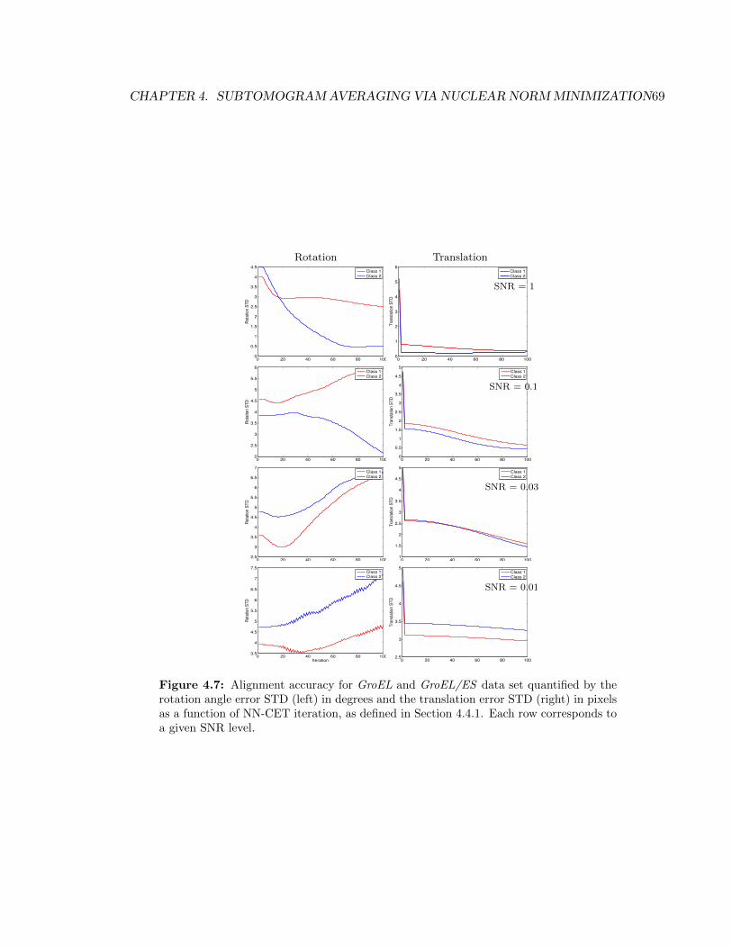
CHAPTER 4. SUBTOMOGRAMAVERAGING VIA NUCLEAR NORMMINIMIZATION69
Rotation Translation
0 20 40 60 80 1000
0.5
1
1.5
2
2.5
3
3.5
4
4.5
Rot
atio
n ST
D
Class 1Class 2
0 20 40 60 80 1000
1
2
3
4
5
6
Tran
slat
ion
STD
Class 1Class 2
SNR = 1
0 20 40 60 80 1002
2.5
3
3.5
4
4.5
5
5.5
6
Rot
atio
n ST
D
Class 1Class 2
0 20 40 60 80 1000
0.5
1
1.5
2
2.5
3
3.5
4
4.5
5
Tran
slat
ion
STD
Class 1Class 2
SNR = 0.1
0 20 40 60 80 1002.5
3
3.5
4
4.5
5
5.5
6
6.5
7
Rot
atio
n ST
D
Class 1Class 2
0 20 40 60 80 1001
1.5
2
2.5
3
3.5
4
4.5
5
Tran
slat
ion
STD
Class 1Class 2
SNR = 0.03
0 20 40 60 80 1003.5
4
4.5
5
5.5
6
6.5
7
7.5
Rot
atio
n ST
D
Iteration
Class 1Class 2
0 20 40 60 80 1002.5
3
3.5
4
4.5
5
Tran
slat
ion
STD
Class 1Class 2
SNR = 0.01
Figure 4.7: Alignment accuracy for GroEL and GroEL/ES data set quantified by therotation angle error STD (left) in degrees and the translation error STD (right) in pixelsas a function of NN-CET iteration, as defined in Section 4.4.1. Each row corresponds toa given SNR level.

CHAPTER 4. SUBTOMOGRAMAVERAGING VIA NUCLEAR NORMMINIMIZATION70
0 0.1 0.2 0.3 0.4 0.50
0.2
0.4
0.6
0.8
1
FSC
SNR = 1
0 0.1 0.2 0.3 0.4 0.50
0.2
0.4
0.6
0.8
1NN−CETML
SNR = 0.1
0 0.1 0.2 0.3 0.4 0.50
0.2
0.4
0.6
0.8
1
FSC
freq
SNR = 0.03
0 0.1 0.2 0.3 0.4 0.50
0.2
0.4
0.6
0.8
1
freq
SNR = 0.01
0 0.1 0.2 0.3 0.4 0.50
0.2
0.4
0.6
0.8
1
FSC
SNR = 1
0 0.1 0.2 0.3 0.4 0.50
0.2
0.4
0.6
0.8
1NN−CETML
SNR = 0.1
0 0.1 0.2 0.3 0.4 0.50
0.2
0.4
0.6
0.8
1
FSC
freq
SNR = 0.03
0 0.1 0.2 0.3 0.4 0.50
0.2
0.4
0.6
0.8
1
freq
SNR = 0.01
Figure 4.8: Fourier shell correlation curves of GroEL (rows 1,2) and GroEL/ES (row3,4) at SNR = 1, 0.1 0.03, and 0.01. The curves are calculated between the ground truthstructure and the 1. NN-CET aligned reconstruction (our method, cyan); 2. ML-TOMOreconstruction (green).

CHAPTER 4. SUBTOMOGRAMAVERAGING VIA NUCLEAR NORMMINIMIZATION71
Helicases
Similar to the GroEL and GroEL/ES case, the reconstruction accuracy for Helicases suffers
from low SNR, as can be seen from Figures 4.9 to 4.11.
The standard deviation of the translation and rotation estimation errors for Helicases
are plotted in Figure 4.12. At SNR = 1, the in-class variation in rotation errors decreases
strongly until around 50 iterations, after which it increases again. When looking at the
pairwise difference between rotation matrix estimation errors, shown in Figure 4.13, we
see that the initial rotation alignment is poor. At iteration 50, the angles between all
pairs of rotation parameter misfits are very small, indicating good alignment. The pairwise
distances do increase again, but overall the level at iteration 100 is still smaller than at
the beginning. This means that although we do not have the most optimal alignment at
iteration = 100, the observations are still relatively better aligned than at the beginning of
the simulations (at iteration = 0) still maintaining the classes all reasonably aligned within
themselves. This particular observation indicates a few issues: 1. the algorithm can find the
well estimated aligned volumes as well as the alignment parameters, however, the current
formulation is not strongly constrained enough to stop at the optimal solution but keep
exploring different solutions when the optimal solution does not lie in a well constrained
region. 2. the current stopping criterion is not able to detect the best aligned moment for
each class. To cope with these issues, one can record the entire solution path and choose the
best solution for an external metric such as FSC. In this section, we provide the simulation
results obtained at iteration 50 for SNR = 1 to compare the best result, and for SNR = 0.1,
0.3 and 0.01, the simulation results are obtained at iteration 100. At SNR = 0.1 and SNR
= 0.03, the STD of rotation parameter errors fluctuate but overall do seem to decrease. At
SNR = 0.01, the proposed method was not able to find the good angular alignment for any
class.
The FSC plots in Figure 4.14 show that NN-CET and ML-TOMO return reconstructions
that have a comparable spatial resolution to each other for SNR as low as 0.03. The

CHAPTER 4. SUBTOMOGRAMAVERAGING VIA NUCLEAR NORMMINIMIZATION72
resolution of the averaged Hel2 of ML-TOMO, however, is much lower than that of NN-
CET due to misclassification as shown in the confusion matrix in Figure 4.15.

CHAPTER 4. SUBTOMOGRAMAVERAGING VIA NUCLEAR NORMMINIMIZATION73
X Y Z
Original
SNR
=1
NN-C
ET
ML
SNR
=0.1
NN-C
ET
ML
SNR
=0.03
NN-C
ET
ML
SNR
=0.01
NN-C
ET
ML
Figure 4.9: XYZ cross sections of the averaged Hel1 structures for different SNR levels.Each column contains X, Y, Z cross sections at the center of each side of the volume.The first row contains the ground truth. The rest of even-numbered rows (2, 4, 6, 8)show the Hel1 reconstructions of NN-CET at SNR = 1, 0.1, 0.03, 0.01 respectively, andthe rest of odd-numbered rows (3, 5, 7, 9) show the Hel1 reconstructions of ML-TOMOat SNR = 1, 0.1, 0.03, 0.01 respectively.

CHAPTER 4. SUBTOMOGRAMAVERAGING VIA NUCLEAR NORMMINIMIZATION74
X Y Z
Original
SNR
=1
NN-C
ET
ML
SNR
=0.1
NN-C
ET
ML
SNR
=0.03
NN-C
ET
ML
SNR
=0.01
NN-C
ET
ML
Figure 4.10: XYZ cross sections of the averaged Hel2 structures for different SNRlevels. Each column contains X, Y, Z cross sections at the center of each side of thevolume. The first row contains the ground truth. The rest of even-numbered rows (2, 4,6, 8) show the Hel2 reconstructions of NN-CET at SNR = 1, 0.1, 0.03, 0.01 respectively,and the rest of odd-numbered rows (3, 5, 7, 9) show the Hel2 reconstructions of ML-TOMO at SNR = 1, 0.1, 0.03, 0.01 respectively.

CHAPTER 4. SUBTOMOGRAMAVERAGING VIA NUCLEAR NORMMINIMIZATION75
X Y Z
Original
NN-C
ET
ML
NN-C
ET
ML
NN-C
ET
ML
NN-C
ET
ML
Figure 4.11: XYZ cross sections of the averaged Hel3 structures for different SNRlevels. Each column contains X, Y, Z cross sections at the center of each side of thevolume. The first row contains the ground truth. The rest of even-numbered rows (2, 4,6, 8) show the Hel3 reconstructions of NN-CET at SNR = 1, 0.1, 0.03, 0.01 respectively,and the rest of odd-numbered rows (3, 5, 7, 9) show the Hel3 reconstructions of ML-TOMO at SNR = 1, 0.1, 0.03, 0.01 respectively.

CHAPTER 4. SUBTOMOGRAMAVERAGING VIA NUCLEAR NORMMINIMIZATION76
Rotation Translation
0 20 40 60 80 1000
0.5
1
1.5
2
2.5
3
3.5
4
Rot
atio
n ST
D
Class 1Class 2Class 3
0 20 40 60 80 1000
0.5
1
1.5
2
2.5
3
3.5
4
4.5
5
Tran
slat
ion
STD
Class 1Class 2Class 3
SNR = 1
0 20 40 60 80 1000
0.5
1
1.5
2
2.5
3
3.5
4
4.5
5
Rot
atio
n ST
D
Class 1Class 2Class 3
0 20 40 60 80 1000
0.5
1
1.5
2
2.5
3
3.5
4
4.5
5
Tran
slat
ion
STD
Class 1Class 2Class 3
SNR = 0.1
0 20 40 60 80 1002
3
4
5
6
7
8
9
Rot
atio
n ST
D
Class 1Class 2Class 3
0 20 40 60 80 1000
1
2
3
4
5
6
Tran
slat
ion
STD
Class 1Class 2Class 3
SNR = 0.03
0 20 40 60 80 1003
4
5
6
7
8
9
10
11
12
13
Rota
tion
STD
Iteration
Class 1Class 2Class 3
0 20 40 60 80 1002
2.5
3
3.5
4
4.5
5
5.5
Tran
slat
ion
STD
Class 1Class 2Class 3
SNR = 0.01
Figure 4.12: Alignment accuracy for Helicases data set quantified by the rotation angleerror STD (left) in degrees and the translation error STD (right) in pixels as a functionof NN-CET iteration, as defined in Section 4.4.1. Each row corresponds to a given SNRlevel.

CHAPTER 4. SUBTOMOGRAMAVERAGING VIA NUCLEAR NORMMINIMIZATION77
Iteration: 1 50 100
Class
1Class
2Class
3
0
5
10
15
20
25
30
35
Figure 4.13: Pairwise angles between the error rotation matrices between observationswithin classes in degrees for Helicases data set at SNR = 1.
4.4.3 Clustering Accuracy
In the previous section, we have seen that the alignment accuracy of the averaged struc-
tures of NN-CET and ML-TOMO is equivalent when ML-TOMO can accurately cluster
subtomograms. However, when ML-TOMO does not cluster instances accurately, those
clusters that do not contain many examples suffer significantly in terms of resolution. Our
algorithm does not explicitly cluster the samples, but provides a row-rank approximation
of the aligned reconstructions. By clustering the columns of the solution matrix X∗ us-
ing k-means, we can assign classes to each sample. By contrast, ML-TOMO explicitly
assigns each sample to a class that maximizes the overall likelihood of observing the data
set. We evaluate the clustering accuracy, which we define to be the percentage of correctly
labeled samples. As shown in Table 4.1, both NN-CET and ML-TOMO cluster GroEL and
GroEL/ES samples with a very high accuracy at SNR = 1 and 0.1, which gradually reduces
as the SNR decreases. For Helicases we see that ML-TOMO is unable to obtain accurate
clustering for any of the SNR levels, whereas our method clusters Helicases without any
error for SNR levels as low as 0.03. This can be attributed to the dimension reduction that
follows from the nuclear-norm minimization. The proposed approach aligns observations
considering the fact that the heterogeneity in the samples has to be much smaller than the

CHAPTER 4. SUBTOMOGRAMAVERAGING VIA NUCLEAR NORMMINIMIZATION78
0 0.1 0.2 0.3 0.4 0.50
0.2
0.4
0.6
0.8
1
FSC
SNR = 1
0 0.1 0.2 0.3 0.4 0.50
0.2
0.4
0.6
0.8
1NN−CETML
SNR = 0.1
0 0.1 0.2 0.3 0.4 0.50
0.2
0.4
0.6
0.8
1FS
C
freq
SNR = 0.03
0 0.1 0.2 0.3 0.4 0.50
0.2
0.4
0.6
0.8
1
freq
SNR = 0.01
0 0.1 0.2 0.3 0.4 0.50
0.2
0.4
0.6
0.8
1
FSC
SNR = 1
0 0.1 0.2 0.3 0.4 0.50
0.2
0.4
0.6
0.8
1NN−CETML
SNR = 0.1
0 0.1 0.2 0.3 0.4 0.50
0.2
0.4
0.6
0.8
1
FSC
freq
SNR = 0.03
0 0.1 0.2 0.3 0.4 0.50
0.2
0.4
0.6
0.8
1
freq
SNR = 0.01
0 0.1 0.2 0.3 0.4 0.50
0.2
0.4
0.6
0.8
1
FSC
SNR = 1
0 0.1 0.2 0.3 0.4 0.50
0.2
0.4
0.6
0.8
1NN−CETML
SNR = 0.1
0 0.1 0.2 0.3 0.4 0.50
0.2
0.4
0.6
0.8
1
FSC
freq
SNR = 0.03
0 0.1 0.2 0.3 0.4 0.50
0.2
0.4
0.6
0.8
1
freq
SNR = 0.01
Figure 4.14: Fourier shell correlation curves of Hel1 (rows 1,2), Hel2 (rows 3,4), Hel3(rows 5,6) at SNR = 1, 0.1 0.03, and 0.01. The curves are calculated between theground truth structure and the 1. NN-CET aligned reconstruction (our method, cyan);2. ML-TOMO reconstruction (green).

CHAPTER 4. SUBTOMOGRAMAVERAGING VIA NUCLEAR NORMMINIMIZATION79
dimension of the space containing the observations. The efficacy of dimension reduction in
clustering tomograms has also been demonstrated in other works, where all subtomograms
are assumed to be aligned [HHM11, YSRR10].
The confusion matrices in Figure 4.15 provide a more detailed analysis on the perfor-
mance of the two different methods. As shown in the first two rows, the confusion matrices
of the instances clustered using NN-CET show a strong diagonal pattern (or permutation
thereof) until the noise level becomes too high (0.01 for Helicases and 0.03 for GroEL
and GroEL/ES). By contrast, the confusion matrices for the instances clustered using ML-
TOMO only show strong diagonal patterns for GroEL and GroEL/ES cases when SNR =
1 and 0.1. For Helicases, ML-TOMO failed to cluster accurately at any of the given SNR
levels even though the correct number of references is provided. Instead, it tends to create
one or two large clusters not three as provided.
By examining the distribution of the singular values in the nuclear-norm minimized
reconstruction X∗, we can also get an insight on the degree of heterogeneity of the sample
set. Singular values can be interpreted as a scaling factor of each orthogonal component
contained in the image space spanned by the reconstructions; the larger the singular value,
the stronger the component. In this light, if we see a set of singular values that are uniform,
this means that the image space contains a variety of structural components, therefore is
more heterogeneous. On the other hand, if we see a set of singular values with only a few
large values and all others small, we conclude that the set will have few distinct structural
components. There are three factors that affect the singular values of a subtomogram
set: 1. the number of different conformations in the set; 2. how well the reconstructions
are aligned; and 3. the amount of noise in the reconstruction. When the tomograms are
not well aligned or contain high level of noise, the singular values will have a rather flat
distribution. On the other hand, if the subtomogram averaging is successful in aligning
the structures and removing the noise, the only factors affecting the distribution of singular
values should be the number of conformation classes in the set and their similarity. As such,
the distribution of singular values provides a good heuristic to determine how well aligned
the samples are and how many distinct classes are present in the dataset. Figure 4.16 shows

CHAPTER 4. SUBTOMOGRAMAVERAGING VIA NUCLEAR NORMMINIMIZATION80
GroEL/ES HelicasesSNR Unaligned X ML Unaligned X ML
1 59% 100% 100% 43% 100% 64%0.1 60% 100% 91% 43% 100% 69%0.03 54% 72% 70% 46% 100% 58%0.01 55% 57% 53% 50% 43% 38%
Table 4.1: Clustering accuracy for GroEL & GroEL/ES and Helicases data sets: Thehighest accuracy for each experiment is highlighted in bold. 1. The unaligned columncontains the accuracy of clustering subtomograms before aligning them. 2. The X columncontains the accuracy of clustering the solved X matrix using the proposed method. 3.The ML column contains the accuracy of labels returned by the Maximum Likelihoodmethod.
the sorted singular values of the nuclear-norm minimized reconstruction X∗ normalized
by the largest singular value on logarithmic scale, and likewise for matrices formed by
concatenating the raw subtomograms before subtomogram averaging (unaligned). For NN-
CET we see that the resulting distribution is extremely sparse with a sharp decrease after
1–3 significant singular values. The number of dominant singular values of GroEL and
GroEL/ES reconstructions at SNR = 1 and 0.1, and for Helicases at SNR = 1, 0.1, and
0.03 matches exactly the true number of conformational classes contained in the data set.
For the unaligned subtomograms prior to any processing, we see that the ten largest
singular values are at most 1–5 times smaller than the largest one. This indicates that the
set is not well aligned and/or severely affected by noise, and it is clearly not possible to
estimate the number of classes from this set of singular values.
In summary, we conclude that the dimension reduction carried out by the nuclear-
norm minimization in NN-CET enables more accurate clustering, and also provides a good
heuristic for determining the number of conformation classes contained in the data. The
procedures used in ML-TOMO do not provide any information equivalent to this.
4.4.4 Computational Complexity and Runtime
The proposed method was implemented in Matlab with a dependency on TFOCS [BCG11]
to solve the sub-problems. The computation was parallelized among 12 cores on a single

CHAPTER 4. SUBTOMOGRAMAVERAGING VIA NUCLEAR NORMMINIMIZATION81
SNR=1 0.1 0.03 0.01
NN-C
ET
GroEL/ES
Helicases
ML-T
OMO
GroEL/ES
Helicases
Figure 4.15: Confusion matrices. Each row contains the breakdown ratio of instancesof each true class into its estimated classes. ith row corresponds to the true class i andjth column corresponds to the estimated class j. Perfect classification is indicated by amatrix with “1.00” on the diagonal and “0.00” everywhere else.
machine, resulting in a per-iteration time of about 275 seconds and an overall runtime of
7.5 hours for 100 iterations. Around 25% of the compute time is spent on evaluating the
nuclear norm and applying singular-value soft thresholding. The remaining 75% is spent
on evaluating the measurement constraint, three-quarters of which was used for evaluating
projections and back-projections using the 3D Radon operator and its adjoint; amounting
to roughly half of the total computation. We ran Xmipp ML-TOMO (version 2.4) on a
single core taking about 36 hours for 20 iterations. The proposed method took around 53
hours for 100 iterations when ran on a single core.
As reflected in the lengthy run time, this initial implementation does not scale up well
to handle high resolution volumes. In our test, the convergence of parameter estimates
for high resolution data sets were also slower especially estimating accurate translation
parameters. This slow convergence and lengthy run time can be overcome by speeding
up the computation intensive 3D Radon operators as well as more efficient nuclear norm
calculation.
The 3D Radon implementation used in the NN-CET solver has a complexity of O(N ·
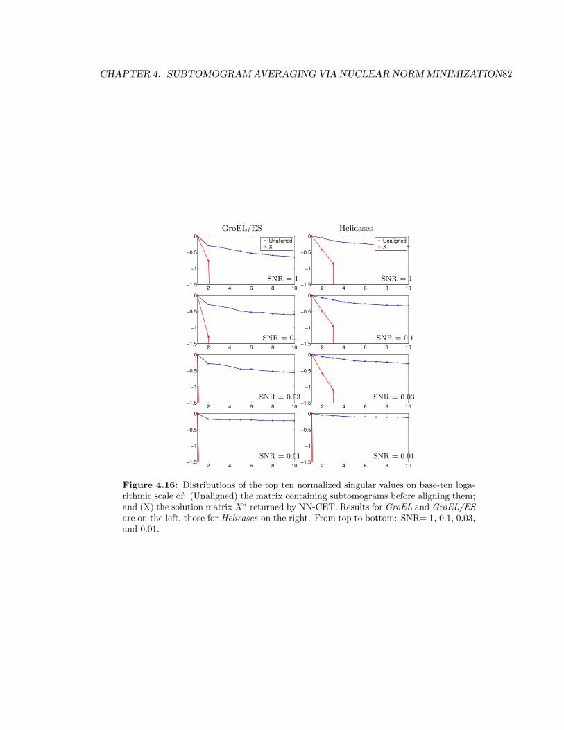
CHAPTER 4. SUBTOMOGRAMAVERAGING VIA NUCLEAR NORMMINIMIZATION82
GroEL/ES Helicases
2 4 6 8 10−1.5
−1
−0.5
0UnalignedX
SNR = 12 4 6 8 10
−1.5
−1
−0.5
0UnalignedX
SNR = 1
2 4 6 8 10−1.5
−1
−0.5
0
SNR = 0.12 4 6 8 10
−1.5
−1
−0.5
0
SNR = 0.1
2 4 6 8 10−1.5
−1
−0.5
0
SNR = 0.032 4 6 8 10
−1.5
−1
−0.5
0
SNR = 0.03
2 4 6 8 10−1.5
−1
−0.5
0
SNR = 0.012 4 6 8 10
−1.5
−1
−0.5
0
SNR = 0.01
Figure 4.16: Distributions of the top ten normalized singular values on base-ten loga-rithmic scale of: (Unaligned) the matrix containing subtomograms before aligning them;and (X) the solution matrix X∗ returned by NN-CET. Results for GroEL and GroEL/ESare on the left, those for Helicases on the right. From top to bottom: SNR= 1, 0.1, 0.03,and 0.01.

CHAPTER 4. SUBTOMOGRAMAVERAGING VIA NUCLEAR NORMMINIMIZATION83
M ·m · s), where, N is the number of volumes, M is the number of projections per volume,
m is the number of samples/observations per projection (number of pixels per projection),
and s is the number of voxels along one side of a 3D cube, thus giving a total of n = s3
voxels. For the Radon operator and its adjoint, processing a single projection line takes O(s)
and can be parallelized over individual volumes as well as projection angles in the forward
case. We therefore expect that the computational cost could be significantly reduced by a
multi-threaded implementation of the Radon operator.
Further reductions in the compute time could be achieved by speeding up the nuclear
norm evaluation, which takes up around 25% of the total compute time. The complexity of
SVD, which is the core operation to evaluate nuclear norms is O(max(a2b, a2b)) for matrices
of size a× b. In our experiments we have a = n and b = N with n > N , giving a complexity
of O(n2 ·N) for evaluating the SVD. Techniques to reduce the computational complexity of
the SVD or methods that avoid it altogether (see for example [WYZ12]) could help further
reduce the compute time of NN-CET.
4.5 Conclusions
In this chapter, we have proposed NN-CET, an approach to the subtomogram averaging
problem based on matrix norm minimization. The proposed approach does not require any
prior information such as the number of classes or references of the target structures. In-
stead, it formulates the alignment and classification problem as a low-rank matrix recovery
problem that explicitly recovers the alignment parameters by calculating the linearized effect
of translation and rotation of the underlying structure on the tomographic measurements.
This approach implicitly addresses the missing wedge issue by formulating tomographic
sensing operators at each projection angle, which is known a priori. The nuclear-norm min-
imized solution matrix spans the principal components of the heterogeneous conformations
embedded in the observed samples, and we can effectively cluster reconstructions in this
low dimensional space.
Our experiments indicate that NN-CET successfully clusters structures during alignment

CHAPTER 4. SUBTOMOGRAMAVERAGING VIA NUCLEAR NORMMINIMIZATION84
and manages to do so more accurately than ML-TOMO. The alignment accuracy of the
averaged structures of NN-CET and ML-TOMO are equivalent for those cases where ML-
TOMO can accurately cluster subtomograms. While our results are promising, there are
a number of issues that need to be addressed before it can be used as a reference free
subtomogram averaging algorithm with high clustering accuracy. The first is computational
cost. While we think our algorithm could easily leverage the parallel computation of a
cluster, we have not yet created a cluster version. The more significant issue is the one of
convergence. Further work is needed to improve the convergence of this algorithm, so larger
data sets can be run, as well as create a better stopping condition, to avoid the issues we
saw when dealing with Helicases.

Chapter 5
Conclusions
CET is an indispensable tool to discover the high resolution structure of the building
blocks of cells and viruses thanks to its capability of imaging in high resolution in 3D. This
success has not been possible without a significant research effort to cope with challenging
image characteristics of CET projections and reconstructions, which are very low SNR and
missing frequency components. The low SNR and contrast of CET images are here to
stay since it is limited by electron dose and voltage that we can apply to organic materials
without damaging it. The missing wedge problem is difficult to overcome as well since the
quality of CET projections are limited by the increase in the thickness of the sample when
it is rotated up to high tilt angles. The longer the path that electrons have to path, the
weaker the phase-contrast signal from the electrons becomes due to the increase in inelastic
scattering. Fortunately, these challenges have been managed by automated acquisition
techniques and image processing pipeline, that enables researchers take large amount of
samples and assemble them into high resolution models of macromolecules at higher SNR.
In this thesis, we have proposed robust image processing enhancements to the CET
image processing pipeline using sparse priors. The idea behind robust image processing
techniques proposed here is that often a single image or a set of images exhibit sparsity pat-
tern in an alternate signal domain. The first example is the digital inpainting algorithm for
CET . Here, we have empirically demonstrated that CET projections are sparse in theDCT
85
CHAPTER 5. CONCLUSIONS 86
domain, and utilized this information to remove high contrast artifacts in the projections
images as well as 3D reconstructions in the CS framework. The algorithm can seamlessly
replace pixels occupied by high contrast objects such as gold markers in projection images.
Then, by reconstructing 3D volume using inpainted projections, we can produce artifact-free
tomograms. By removing high contrast artifacts casting shadow on specimens of interest,
we can study them with greater clarity as well as analyze them analytically with more
confidence. Artificial marker test and subtomogram averaging test have confirmed that the
proposed method preserves the structural integrity of the unpainted regions and their neigh-
boring regions free from artifacts better than the conventional inpainting methods used in
the CET community.
The presented method inpaints each individual projection separately, because this al-
lowed us to create a number of large, but tractable optimization problems. Unfortunately
optimizing each projection separately does not exactly solve the desired problem because
each optimization can result in an inpainted projection that is not necessarily consistent
with the 3D structure of a specimen, creating secondary inpainting artifacts. One straight-
forward application of CS techniques to provide a tomogram that is free from artifacts and
consistent with 3D structural information of a specimen can be jointly minimizing the 2D
sparsity of all projections in the DCT domain as well as the 3D sparsity in the Fourier
domain if applicable. However, this approach is not yet computationally tractable.
Another example of sparsity utilizing robust image processing technique demonstrated
in this thesis is a batch alignment and clustering algorithm for subtomograms. In this
case, we utilized the fact that a set of well aligned images span a low dimensional space.
Even a set of images containing multiple classes, if they are all well aligned within each
class, the whole image space spanned by these images should be as low dimension as the
number of classes. This means that an image matrix whose columns are vectorized version
of a subtomogram should have a low rank if all subtomograms are aligned within each
class. Utilizing this information, we framed the subtomogram averaging problem, basically
a simultaneous batch alignment and clustering problem, into a matrix norm minimization
problem, that can align and cluster subtomograms without prior references nor the number

CHAPTER 5. CONCLUSIONS 87
of class information. This feature, that we do not have to impose a prior class information,
is very unique, since all subtomogram algorithms currently being used in the CET commu-
nity require one or both of this information. However, using prior references can bias the
resulting averaged structure. In our limited scale simulations, we have demonstrated that
this algorithm can efficiently produce clustered and aligned averaged models from noisy
and missing-wedge corrupted tomograms even using only a small number of observations.
The resulting averaged structure produced by the proposed method has higher FSC than
ones produced by the benchmark method. However, this algorithm has been only evaluated
using synthetic data sets, and it needs to be fully evaluated on large scale high resolution
real data set to prove its efficacy in the field.
Although, both examples in this thesis demonstrated positive opportunities for sparsity
inspired image processing algorithms for robust CET image analysis, there are a few im-
provements that can enhance these algorithms and be widely used on a large set of CET
images. One of the most significant improvement can come from expediting convex pro-
gramming used in these algorithms. Currently, l1 norm minimization used in the digital
inpainting algorithm can be solved quite quickly, therefore, the computational complexity is
less of a concern here. However, subtomogram averaging problem can be quite large. For ex-
ample, these days it has become quite common to align a set of 1000 or more high resolution
subtomograms of size 128× 128× 128 and to solve this scale of matrix norm minimization
problem, the current solver requires large amount of memory in addition to many compute
cores to solve large scale SVD and to evaluate each subtomogram’s measurement require-
ments. Fortunately, there are interesting developments in distributed memory computing
for large scale dense linear algebra [PMvdG+13, BCC+97] as well as GPU processing[LN09],
so this problem may become feasible in the near future.

Bibliography
[ACN+10] Fernando Amat, Luis R. Comolli, John F. Nomellini, Farshid Moussavi, Ken-
neth H. Downing, John Smit, and Mark Horowitz. Analysis of the intact
surface layer of Caulobacter crescentus by cryo-electron tomography. Journal
of Bacteriology, 192(22):5855–5865, 2010.
[AK84] A.H. Andersen and A.C. Kak. Simultaneous algebraic reconstruction tech-
nique (sart): A superior implementation of the {ART} algorithm. Ultrasonic
Imaging, 6(1):81 – 94, 1984.
[AMC+08] Fernando Amat, Farshid Moussavi, Luis R. Comolli, Gal Elidan, Kenneth H.
Downing, and Mark Horowitz. Markov random field based automatic image
alignment for electron tomography. Journal of Structural Biology, 161(3):260
– 275, 2008. The 4th International Conference on Electron TomographyThe
4th International Conference on Electron Tomography.
[BBC+01] C. Ballester, M. Bertalmio, V. Caselles, G. Sapiro, and J. Verdera. Filling-in
by joint interpolation of vector fields and gray levels. Image Processing, IEEE
Transactions on, 10(8):1200–1211, August 2001.
[BBC11] Stephen Becker, Jerome Bobin, and Emmanuel J. Candes. Nesta: A fast and
accurate first-order method for sparse recovery. SIAM Journal on Imaging
Sciences, 4(1):1–39, 2011.
88

BIBLIOGRAPHY 89
[BCC+97] L Susan Blackford, Jaeyoung Choi, Andy Cleary, Eduardo D’Azevedo, James
Demmel, Inderjit Dhillon, Jack Dongarra, Sven Hammarling, Greg Henry,
Antoine Petitet, et al. ScaLAPACK users’ guide, volume 4. siam, 1997.
[BCG+10] Grant R. Bowman, Luis R. Comolli, Guido M. Gaietta, Michael Fero, Sun-
Hae Hong, and et al. Caulobacter popz forms a polar subdomain dictating
sequential changes in pole composition and function. Molecular Microbiology,
76(1):173–189, 2010.
[BCG11] Stephen Becker, Emmanuel J. Candes, and Michael Grant. Templates for con-
vex cone problems with applications to sparse signal recovery. Mathematical
Programming Computation, 3(3), 2011.
[BHE01] Sami Brandt, Jukka Heikkonen, and Peter Engelhardt. Multiphase method
for automatic alignment of transmission electron microscope images using
markers. Journal of Structural Biology, 133(1):10 – 22, 2001.
[BJ03] R. Basri and D.W. Jacobs. Lambertian reflectance and linear subspaces. Pat-
tern Analysis and Machine Intelligence, IEEE Transactions on, 25(2):218–
233, Feb 2003.
[BNR+12] Tanmay A. M. Bharat, Takeshi Noda, James D. Riches, Verena Kraehling,
Larissa Kolesnikova, Stephan Becker, Yoshihiro Kawaoka, and John A. G.
Briggs. Structural dissection of Ebola virus and its assembly determinants
using cryo-electron tomography. Proceedings of the National Academy of Sci-
ences of the United States of America, 109(11):4275–4280, 2012.
[Bra56] R. N. Bracewell. Strip integration in radio astronomy. Australian Journal of
Physics, 9:198–217, 1956.
[Bro92] Lisa Gottesfeld Brown. A survey of image registration techniques. ACM
Computing Surveys, 24(4):325–376, 1992.

BIBLIOGRAPHY 90
[BS09] Alberto Bartesaghi and Sriram Subramaniam. Membrane protein structure
determination using cryo-electron tomography and 3D image averaging. Cur-
rent Opinion in Structural Biology, 19(4):402–407, 2009.
[BSL+08] A. Bartesaghi, P. Sprechmann, J. Liu, G. Randall, G. Sapiro, and S. Subra-
maniam. Classification and 3D averaging with missing wedge correction in
biological electron tomography. Journal of Structural Biology, 162(3):436–
450, 2008.
[BT09a] Amir Beck and Marc Teboulle. A fast iterative shrinkage-thresholding al-
gorithm for linear inverse problems. SIAM Journal on Imaging Sciences,
2(1):183–202, 2009.
[BT09b] Amir Beck and Marc Teboulle. A fast iterative shrinkage-thresholding algo-
rithm with application to wavelet-based image deblurring. In International
Conference on Acoustics, Speech and Signal Processing, pages 693–696, 2009.
[BVSO03] M. Bertalmio, L. Vese, G. Sapiro, and S. Osher. Simultaneous structure and
texture image inpainting. Image Processing, IEEE Transactions on, 12(8):882
– 889, 2003.
[CDS98] Scott Shaobing Chen, David L. Donoho, and Michael A. Saunders. Atomic
decomposition by basis pursuit. SIAM J. Sci. Comput., 20:33–61, December
1998.
[CDSAAF10] Daniel Castao-Dez, Margot Scheffer, Ashraf Al-Amoudi, and Achilleas S.
Frangakis. Alignator: A {GPU} powered software package for robust fiducial-
less alignment of cryo tilt-series. Journal of Structural Biology, 170(1):117 –
126, 2010.
[CKS02] Tony F. Chan, Sung Ha Kang, and Jianhong Shen. Euler’s elastica
and curvature-based inpainting. SIAM Journal on Applied Mathematics,
63(2):564–592, 2002.
BIBLIOGRAPHY 91
[CLMW11] Emmanuel J Candes, Xiaodong Li, Yi Ma, and John Wright. Robust principal
component analysis? Journal of the ACM (JACM), 58(3):11, 2011.
[ClTCB11] Ricardo S. Cabral, Fernando D. De la Torre, Joao P. Costeira, and Alexan-
dre Bernardino. Matrix completion for multi-label image classification. In
J. Shawe-Taylor, R.S. Zemel, P. Bartlett, F.C.N. Pereira, and K.Q. Wein-
berger, editors, Advances in Neural Information Processing Systems 24, pages
190–198. 2011.
[CPH+13] Yuxiang Chen, Stefan Pfeffer, Thomas Hrabe, Jan Michael Schuller, and
Friedrich Forster. Fast and accurate reference-free alignment of subtomo-
grams. Journal of Structural Biology, 182(3):235–245, 2013.
[CRT06a] E.J. Candes, J. Romberg, and T. Tao. Robust uncertainty principles: exact
signal reconstruction from highly incomplete frequency information. Infor-
mation Theory, IEEE Transactions on, 52(2):489 – 509, 2006.
[CRT06b] Emmanuel J. Candes, Justin Romberg, and Terence Tao. Robust uncertainty
principles: Exact signal reconstruction from highly incomplete frequency in-
formation. IEEE Transactions on Information Theory, 52(2):489–509, 2006.
[CRT06c] Emmanuel J. Candes, Justin K. Romberg, and Terence Tao. Stable signal
recovery from incomplete and inaccurate measurements. Communications on
Pure and Applied Mathematics, 59(8):1207–1223, August 2006.
[CS01] Tony F. Chan and Jianhong Shen. Mathematical models for local nontexture
inpaintings. SIAM Journal on Applied Mathematics, 62(3):1019–1043, 2001.
[CT06] Emmanuel J. Candes and Terence Tao. Near-optimal signal recovery from
random projections – universal encoding strategies. IEEE Transactions on
Information Theory, 52(2), 2006.

BIBLIOGRAPHY 92
[DFG+09] Elia Diestra, Juan Fontana, Paul Guichard, Sergio Marco, and Cristina Risco.
Visualization of proteins in intact cells with a clonable tag for electron mi-
croscopy. Journal of Structural Biology, 165(3):157 – 168, 2009.
[DK68] DJ DeRosier and A Klug. Reconstruction of three dimensional structures
from electron micrographs. Nature, 217(5124):130–134, 1968.
[DKMN10] Radostin Danev, Shuji Kanamaru, Michael Marko, and Kuniaki Nagayama.
Zernike phase contrast cryo-electron tomography. Journal of Structural Biol-
ogy, 171(2):174 – 181, 2010.
[DND+00] B. De Man, J. Nuyts, P. Dupont, G. Marchal, and P. Suetens. Reduction
of metal streak artifacts in x-ray computed tomography using a transmission
maximum a posteriori algorithm. Nuclear Science, IEEE Transactions on,
47(3):977–981, June 2000.
[Don06] David L. Donoho. Compressed sensing. IEEE Transactions on Information
Theory, 52(4):1289–1306, 2006.
[emd] Emdatabank. http://emdatabank.org/.
[ESQD05] M. Elad, J.-L. Starck, P. Querre, and D.L. Donoho. Simultaneous cartoon
and texture image inpainting using morphological component analysis (mca).
Applied and Computational Harmonic Analysis, 19(3):340 – 358, 2005.
[Fer12] Jose-Jesus Fernandez. Computational methods for electron tomography. Mi-
cron, 43(10):1010–1030, 2012.
[FH01] Achilleas S. Frangakis and Reiner Hegerl. Noise reduction in electron to-
mographic reconstructions using nonlinear anisotropic diffusion. Journal of
Structural Biology, 135(3):239 – 250, 2001.
[FHB01] Maryam Fazel, Haitham Hindi, and Stephen P Boyd. A rank minimiza-
tion heuristic with application to minimum order system approximation. In
BIBLIOGRAPHY 93
American Control Conference, 2001. Proceedings of the 2001, volume 6, pages
4734–4739. IEEE, 2001.
[FL05] J.-J. Fernndez and S. Li. Anisotropic nonlinear filtering of cellular structures
in cryoelectron tomography. Computing in Science and Engineering, 7(5):54–
61, 2005. cited By 24.
[FLC06] J.J. Fernndez, S. Li, and R.A. Crowther. {CTF} determination and correction
in electron cryotomography. Ultramicroscopy, 106(7):587 – 596, 2006.
[FMZ+05] Friedrich Forster, Ohad Medalia, Nathan Zauberman, Wolfgang Baumeister,
and Deborah Fass. Retrovirus envelope protein complex structure in situ
studied by cryo-electron tomography. Proceedings of the National Academy
of Sciences of the United States of America, 102(13):4729–4734, 2005.
[Fra06] J. Frank. Electron Tomography: Methods for Three-dimensional Visualization
of Structures in the Cell. Second Edition. Springer, 2006.
[GBH70] Richard Gordon, Robert Bender, and Gabor T. Herman. Algebraic recon-
struction techniques (art) for three-dimensional electron microscopy and x-
ray photography. Journal of Theoretical Biology, 29(3):471 – 481, 1970.
[GCSZ11] Hao Gao, Jian-Feng Cai, Zuowei Shen, and Hongkai Zhao. Robust principal
component analysis-based four-dimensional computed tomography. Physics
in Medicine and Biology, 56(11):3181–3198, 2011.
[GJ12] Lu Gan and Grant J. Jensen. Electron tomography of cells. Quarterly Reviews
of Biophysics, 45:27–56, 2012.
[GZY+06] Jianwei Gu, Li Zhang, Guoqiang Yu, Yuxiang Xing, and Zhiqiang Chen. X-
ray ct metal artifacts reduction through curvature based sinogram inpainting.
Journal of X-ray Science and Technology, 14:73–82, 2006.
BIBLIOGRAPHY 94
[HCWS08] J. Bernard Heymann, Giovanni Cardone, Dennis C. Winkler, and Alasdair C.
Steven. Computational resources for cryo-electron tomography in bsoft. Jour-
nal of Structural Biology, 161(3):232–242, 2008.
[HHM11] John M. Heumann, Andreas Hoenger, and David N. Mastronarde. Clustering
and variance maps for cryo-electron tomography using wedge-masked differ-
ences. Journal of Structural Biology, 175(3):288–299, 2011.
[HvH86] G. Harauz and M. van Heel. Exact filters for general geometry three dimen-
sional reconstruction. Optik, 73(4):146–156, 1986.
[JB07] Grant J Jensen and Ariane Briegel. How electron cryotomography is opening
a new window onto prokaryotic ultrastructure. Current Opinion in Structural
Biology, 17(2):260–267, 2007.
[KCW+10] Mikhail Kudryashev, Marek Cyrklaff, Reinhard Wallich, Wolfgang Baumeis-
ter, and Friedrich Frischknecht. Distinct in situ structures of the Borrelia
flagellar motor. Journal of Structural Biology, 169(1):54–61, 2010.
[KFB+13] Oleg Kuybeda, Gabriel A. Frank, Alberto Bartesaghi, Mario Borgnia, Sri-
ram Subramaniam, and Guillermo Sapiro. A collaborative framework for
3D alignment and classification of heterogeneous subvolumes in cryo-electron
tomography. Journal of Structural Biology, 181(2):116–127, 2013.
[KMM96] James R. Kremer, David N. Mastronarde, and J. Richard McIntosh. Com-
puter visualization of three-dimensional image data using IMOD. Journal of
Structural Biology, 116(1):71–76, 1996.
[KS01] Avinash C.. Kak and Malcolm Slaney. Principles of computerized tomographic
imaging. Society for Industrial and Applied Mathematics, 2001.
[KWS08] Cezar M. Khursigara, Xiongwu Wu, and Sriram Subramaniam. Chemore-
ceptors in caulobacter crescentus: Trimers of receptor dimers in a partially

BIBLIOGRAPHY 95
ordered hexagonally packed array. Journal of Bacteriology, 190(20):6805–
6810, 2008.
[KWZ+08] Cezar M. Khursigara, Xiongwu Wu, Peijun Zhang, Jonathan Lefman, and
Sriram Subramaniam. Role of hamp domains in chemotaxis signaling by
bacterial chemoreceptors. Proceedings of the National Academy of Sciences,
105(43):16555–16560, 2008.
[LDP07] Michael Lustig, David Donoho, and John M. Pauly. Sparse mri: The appli-
cation of compressed sensing for rapid mr imaging. Magnetic Resonance in
Medicine, 58(6):1182–1195, December 2007.
[LFB05] Vladan Lucic, Friedrich Forster, and Wolfgang Baumeister. Structural studies
by electron tomography: from cells to molecules. Annual Review of Biochem-
istry, 74(1):833–865, 2005.
[LJ09] Zhuo Li and Grant J Jensen. Electron cryotomography: a new view into
microbial ultrastructure. Current Opinion in Microbiology, 12(3):333–340,
2009.
[LN09] Sheetal Lahabar and PJ Narayanan. Singular value decomposition on gpu
using cuda. In Parallel & Distributed Processing, 2009. IPDPS 2009. IEEE
International Symposium on, pages 1–10. IEEE, 2009.
[lTB03] Fernando De la Torre and Michael J. Black. Robust parameterized component
analysis: theory and applications to 2D facial appearance models. Computer
Vision and Image Understanding, 91(1–2):53–71, 2003.
[MD07] Christopher P. Mercogliano and David J. DeRosier. Concatenated metalloth-
ionein as a clonable gold label for electron microscopy. Journal of Structural
Biology, 160(1):70 – 82, 2007.
[MHA+10] Farshid Moussavi, Geremy Heitz, Fernando Amat, Luis R. Comolli, Daphne
Koller, and Mark Horowitz. 3d segmentation of cell boundaries from whole

BIBLIOGRAPHY 96
cell cryogenic electron tomography volumes. Journal of Structural Biology,
170(1):134 – 145, 2010.
[MHL+05] W. Moss, S. Haase, J.M. Lyle, D.A. Agard, and J.W. Sedat. A novel 3d
wavelet-based filter for visualizing features in noisy biological data. Journal
of Microscopy, 219(2):43–49, 2005. cited By 13.
[MJCD08] Raghu Meka, Prateek Jain, Constantine Caramanis, and Inderjit S. Dhillon.
Rank minimization via online learning. In ICML, pages 656–663, 2008.
[MLJ06] Gavin E Murphy, Jared R Leadbetter, and Grant J Jensen. In situ structure
of the complete treponema primitia flagellar motor. Nature, 442(7106):1062–
1064, 2006.
[MNM04] Richard McIntosh, Daniela Nicastro, and David Mastronarde. New views of
cells in 3D: an introduction to electron tomography. Trends in cell biology,
15(1):43–51, 2004.
[Moa02] Maher Moakher. Means and averaging in the group of rotations. SIAM
journal on matrix analysis and applications, 24(1):1–16, 2002.
[MS09] Jacqueline L. S. Milne and Sriram Subramaniam. Cryo-electron tomogra-
phy of bacteria: progress, challenges and future prospects. Nature Reviews
Microbiology, 7(9):666–675, 2009.
[MSGA+14] Antonio Martinez-Sanchez, Inmaculada Garcia, Shoh Asano, Vladan Lucic,
and Jose-Jesus Fernandez. Robust membrane detection based on tensor vot-
ing for electron tomography. Journal of Structural Biology, 186(1):49 – 61,
2014.
[MSGF13] Antonio Martinez-Sanchez, Inmaculada Garcia, and Jose-Jesus Fernandez. A
ridge-based framework for segmentation of 3d electron microscopy datasets.
Journal of Structural Biology, 181(1):61 – 70, 2013.
BIBLIOGRAPHY 97
[NAB+08] Rajesh Narasimha, Iman Aganj, Adam E. Bennett, Mario J. Borgnia, Daniel
Zabransky, Guillermo Sapiro, Steven W. McLaughlin, Jacqueline L.S. Milne,
and Sriram Subramaniam. Evaluation of denoising algorithms for biological
electron tomography. Journal of Structural Biology, 164(1):7 – 17, 2008.
[NRRM+06] Rafael Nunez-Ramrez, Yolanda Robledo, Pablo Mesa, Silvia Ayora, Juan Car-
los Alonso, Jos Mara Carazo, and Luis Enrique Donate. Quaternary poly-
morphism of replicative Helicase G40P: structural mapping and domain re-
arrangement. Journal of Molecular Biology, 357(4):1063–1076, 2006.
[NSP+06] Daniela Nicastro, Cindi Schwartz, Jason Pierson, Richard Gaudette, Mary E.
Porter, and J. Richard McIntosh. The molecular architecture of axonemes
revealed by cryoelectron tomography. Science, 313(5789):944–948, 2006.
[OFK+06] Julio O. Ortiz, Friedrich Frster, Julia Krner, Alexandros A. Linaroudis, and
Wolfgang Baumeister. Mapping 70s ribosomes in intact cells by cryoelec-
tron tomography and pattern recognition. Journal of Structural Biology,
156(2):334 – 341, 2006.
[PGW+12] Yigang Peng, Arvind Ganesh, John Wright, Wenli Xu, and Yi Ma. RASL: Ro-
bust alignment via sparse and low-rank decomposition for linearly correlated
images. IEEE Transactions on Pattern Analysis and Machine Intelligence,
34(11):2233–2246, 2012.
[PL09] J. Provost and F. Lesage. The application of compressed sensing for photo-
acoustic tomography. Medical Imaging, IEEE Transactions on, 28(4):585
–594, 2009.
[PMV03] J.P.W. Pluim, J.B.A. Maintz, and M.A. Viergever. Mutual-information-based
registration of medical images: a survey. IEEE Transactions on Medical
Imaging, 22(8):986–1004, 2003.

BIBLIOGRAPHY 98
[PMvdG+13] Jack Poulson, Bryan Marker, Robert A. van de Geijn, Jeff R. Hammond, and
Nichols A. Romero. Elemental: A new framework for distributed memory
dense matrix computations. ACM Trans. Math. Softw., 39(2):13:1–13:24,
February 2013.
[RFP10] Benjamin Recht, Maryam Fazel, and Pablo A. Parrilo. Guaranteed minimum-
rank solutions of linear matrix equations via nuclear norm minimization.
SIAM Review, 52(3):471–501, 2010.
[RFR+01] Neil A. Ranson, George W. Farr, Alan M. Roseman, Brent Gowen, Wayne A.
Fenton, Arthur L. Horwich, and Helen R. Saibil. ATP-bound states of GroEL
captured by cryo-electron microscopy. Cell, 107(7):869–879, 2001.
[RGH+12] Alexander Rigort, David Gnther, Reiner Hegerl, Daniel Baum, Britta Weber,
Steffen Prohaska, Ohad Medalia, Wolfgang Baumeister, and Hans-Christian
Hege. Automated segmentation of electron tomograms for a quantitative de-
scription of actin filament networks. Journal of Structural Biology, 177(1):135
– 144, 2012. Ueli Aebi Festschrift.
[RK08] L. Reimer and H. Kohl. Transmission Electron Microscopy, Fifth Edition.
Springer Series in Optical Sciences. Springer, 2008.
[SB08] Michael F. Schmid and Christopher R. Booth. Methods for aligning and
for averaging 3D volumes with missing data. Journal of Structural Biology,
161(3):243–248, 2008.
[SED05] J.-L. Starck, M. Elad, and D.L. Donoho. Image decomposition via the combi-
nation of sparse representations and a variational approach. Image Processing,
IEEE Transactions on, 14(10):1570 –1582, Oct. 2005.
[SHR+15] Florian K. M. Schur, Wim J. H. Hagen, Michaela Rumlova, Tomas Ruml,
Barbara Muller, Hans-Georg Krausslich, and John A. G. Briggs. Structure
BIBLIOGRAPHY 99
of the immature HIV-1 capsid in intact virus particles at 8.8 A resolution.
Nature, 517:505–508, 2015.
[SME+09] Carlos OS Sorzano, Cedric Messaoudi, Matthias Eibauer, Jose Roman Bilbao-
Castro, Reiner Hegerl, S Nickell, Sergio Marco, and Jose Marıa Carazo.
Marker-free image registration of electron tomography tilt-series. BMC bioin-
formatics, 10(1):124, 2009.
[SMVC09] Sjors H.W. Scheres, Roberto Melero, Mikel Valle, and Jose-Maria Carazo.
Averaging of electron subtomograms and random conical tilt reconstructions
through likelihood optimization. Structure, 17(12):1563–1572, 2009.
[SMVM+04] C.O.S. Sorzano, R. Marabini, J. Velazquez-Muriel, J.R. Bilbao-Castro,
S.H.W. Scheres, J.M. Carazo, and A. Pascual-Montano. Xmipp: a new gen-
eration of an open-source image processing package for electron microscopy.
Journal of Structural Biology, 148(2):194–204, 2004.
[TM02] D.S. Taubman and M.W. Marcellin. JPEG 2000: Image Compression Funda-
mentals, Standards and Practice. Kluwer International Series in Engineering
and Computer Science, 2002.
[VGS08] A. Vedaldi, G. Guidi, and S. Soatto. Joint data alignment up to (lossy)
transformations. In Proceedings of the IEEE Conference on Computer Vision
and Pattern Recognition, pages 1–8, June 2008.
[vHF81] Marin van Heel and Joachim Frank. Use of multivariate statistics in analysing
the images of biological macromolecules. Ultramicroscopy, 6(2):187–194, 1981.
[Vol02] Niels Volkmann. A novel three-dimensional variant of the watershed trans-
form for segmentation of electron density maps. Journal of Structural Biology,
138(12):123 – 129, 2002.

BIBLIOGRAPHY 100
[VSS+11] Lenard M. Voortman, Sjoerd Stallinga, Remco H.M. Schoenmakers, Lucas J.
van Vliet, and Bernd Rieger. A fast algorithm for computing and cor-
recting the {CTF} for tilted, thick specimens in {TEM}. Ultramicroscopy,
111(8):1029 – 1036, 2011.
[Win07] Hanspeter Winkler. 3D reconstruction and processing of volumetric data
in cryo-electron tomography. Journal of Structural Biology, 157(1):126–137,
2007.
[WK04] Oliver Watzke and WilliA. Kalender. A pragmatic approach to metal ar-
tifact reduction in ct: merging of metal artifact reduced images. European
Radiology, 14:849–856, 2004.
[WML11] Qing Wang, Christopher P. Mercogliano, and Jan Lwe. A ferritin-based label
for cellular electron cryotomography. Structure, 19(2):147 – 154, 2011.
[WN12] Christian Wachinger and Nassir Navab. Entropy and Laplacian images: struc-
tural representations for multi-modal registration. Medical Image Analysis,
16(1):1–17, 2012.
[WSOV96] Ge Wang, D.L. Snyder, J.A. O’Sullivan, and M.W. Vannier. Iterative deblur-
ring for ct metal artifact reduction. Medical Imaging, IEEE Transactions on,
15(5):657–664, October 1996.
[WYG+09] J. Wright, A.Y. Yang, A. Ganesh, S.S. Sastry, and Yi Ma. Robust face recog-
nition via sparse representation. Pattern Analysis and Machine Intelligence,
IEEE Transactions on, 31(2):210–227, Feb 2009.
[WYZ12] Zaiwen Wen, Wotao Yin, and Yin Zhang. Solving a low-rank factorization
model for matrix completion by a nonlinear successive over-relaxation algo-
rithm. Mathematical Programming Computation, 4(4):333–361, 2012.
[XBA12] Min Xu, Martin Beck, and Frank Alber. High-throughput subtomogram
alignment and classification by Fourier space constrained fast volumetric

BIBLIOGRAPHY 101
matching. Journal of Structural Biology, 178(2):152–164, 2012. Special Issue:
Electron Tomography.
[XMS+09] Quanren Xiong, Mary K. Morphew, Cindi L. Schwartz, Andreas H. Hoenger,
and David N. Mastronarde. {CTF} determination and correction for low dose
tomographic tilt series. Journal of Structural Biology, 168(3):378 – 387, 2009.
[XRY+05] Dan Xia, John C. Roeske, Lifeng Yu, Charles A. Pelizzari, Arno J. Mundt,
and et al. A hybrid approach to reducing computed tomography metal arti-
facts in intracavitary brachytherapy. Brachytherapy, 4(1):18–23, 2005.
[YSRR10] Lingbo Yu, Robert R. Snapp, Teresa Ruiz, and Michael Radermacher. Proba-
bilistic principal component analysis with expectation maximization (PPCA-
EM) facilitates volume classification and estimates the missing data. Journal
of Structural Biology, 171(1):18–30, 2010.
[ZF03] Barbara Zitova and Jan Flusser. Image registration methods: a survey. Image
and Vision Computing, 21(11):977–1000, 2003.
[ZGLM12] Zhengdong Zhang, Arvind Ganesh, Xiao Liang, and Yi Ma. Tilt: Trans-
form invariant low-rank textures. International Journal of Computer Vision,
99(1):1–24, 2012.
[ZLBJ+06] Ping Zhu, Jun Liu, Julian Bess Jr, Elena Chertova, Jeffrey D. Lifson, Henry
Gris, Gilad A. Ofek, Kenneth A. Taylor, and Kenneth H. Roux. Distribu-
tion and three-dimensional structure of AIDS virus envelope spikes. Nature,
441(7095):847–852, 2006.
[ZRW+00] S. Zhao, D.D. Robeltson, G. Wang, B. Whiting, and K.T. Bae. X-ray ct
metal artifact reduction using wavelets: an application for imaging total hip
prostheses. Medical Imaging, IEEE Transactions on, 19(12):1238–1247, 2000.

BIBLIOGRAPHY 102
[ZWX10] Xiaomeng Zhang, Jing Wang, and Lei Xing. Metal artifact reduction in
computed tomography by constrained optimization. Medical Imaging 2010:
Physics of Medical Imaging, 7622(1):76221T, 2010.


![Coronavirus What You Need to Know · 2020-07-03 · electron tomography and cryo-electron microscopy [2,3]. 50 Range is -200nm ... The Ebola virus can survive on doorknobs and countertops](https://img.dokumen.tips/doc/110x75/5f7780fa8f7d42096e0a27b3/coronavirus-what-you-need-to-know-2020-07-03-electron-tomography-and-cryo-electron.jpg)