Embed Size (px)
Citation preview

Robust adaptive nonlinear control of microgrid frequency and voltage in the presence of renewable energy sources
by
Hamed TAHERI LEDARI
THESIS PRESENTED TO ÉCOLE DE TECHNOLOGIE SUPÉRIEURE
IN PARTIAL FULFILLMENT OF THE REQUIREMENTS FOR THE DEGREE OF DOCTOR OF PHILOSOPHY
PH.D.
MONTRÉAL, JULY 19, 2017
ÉCOLE DE TECHNOLOGIE SUPÉRIEURE UNIVERSITÉ DU QUÉBEC
© Copyright 2017 reserved by Hamed Taheri Ledari

© Copyright reserved
It is forbidden to reproduce, save or share the content of this document either in whole or in parts. The reader
who wishes to print or save this document on any media must first get the permission of the author.
BOARD OF EXAMINERS
THIS THESIS HAS BEEN EVALUATED
BY THE FOLLOWING BOARD OF EXAMINERS : Dr. Ouassima Akhrif, Thesis Supervisor Département de génie électrique at École de technologie supérieure Dr. Aimé Francis Okou, Thesis Co-supervisor Department of electrical and computer engineering at Royal Military Collage of Canada Dr. Roger Champagne, Committee President Département de génie logiciel et TI at École de technologie supérieure Dr. Handy Fortin Blanchette, Examiner Département de génie électrique at École de technologie supérieure Dr. Guy Gauthier, Examiner Département de génie de la production automatisée at École de technologie supérieure Dr. Mohammed El Kahel, Independent External Examiner GE Renewable Energy
THIS THESIS WAS PRENSENTED AND DEFENDED
IN THE PRESENCE OF A BOARD OF EXAMINERS AND THE PUBLIC
ON MARCH 21, 2017
AT ÉCOLE DE TECHNOLOGIE SUPÉRIEURE


ACKNOWLEDGMENT
This research would not have been possible without the support of many people. I would like
to express my deepest gratitude to my supervisor of studies, Prof. Ouassima Akhrif, for
giving me the opportunity to undertake this research work and for her supervision, expertise,
guidance and support during the entire project.
I would like to express my gratitude and respect to my co-supervisor Prof. Aime Francis
Okou for his guidance, support and trust during my Ph.D. program.
Many thanks go in particular to Dr. Mohammed El Kahel, Prof. Handy Fortin Blanchette,
Prof. Guy Gauthier and Prof. Roger Champagne for accepting to be jury members and for
their constructive criticism which contributed to improve the quality of this thesis.
I would like to thank all personnel in the GRÉPCI group for their cooperation, moral as well
as technical support and encouragement.
And, last but not least, I wish to express my deepest love and gratitude to my beloved parents
and my family for their understanding, patience and endless love and also my friends for
their help and support throughout the duration of my Ph.D. studies.

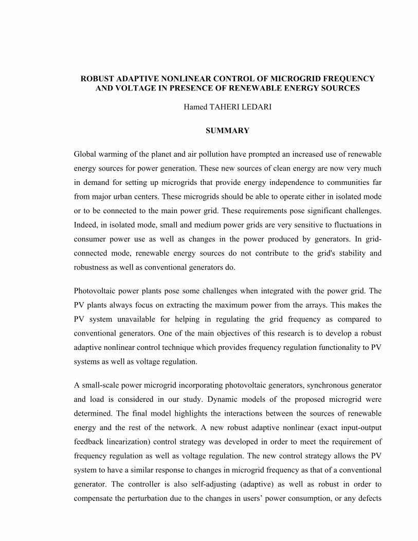
ROBUST ADAPTIVE NONLINEAR CONTROL OF MICROGRID FREQUENCY AND VOLTAGE IN PRESENCE OF RENEWABLE ENERGY SOURCES
Hamed TAHERI LEDARI
SUMMARY
Global warming of the planet and air pollution have prompted an increased use of renewable
energy sources for power generation. These new sources of clean energy are now very much
in demand for setting up microgrids that provide energy independence to communities far
from major urban centers. These microgrids should be able to operate either in isolated mode
or to be connected to the main power grid. These requirements pose significant challenges.
Indeed, in isolated mode, small and medium power grids are very sensitive to fluctuations in
consumer power use as well as changes in the power produced by generators. In grid-
connected mode, renewable energy sources do not contribute to the grid's stability and
robustness as well as conventional generators do.
Photovoltaic power plants pose some challenges when integrated with the power grid. The
PV plants always focus on extracting the maximum power from the arrays. This makes the
PV system unavailable for helping in regulating the grid frequency as compared to
conventional generators. One of the main objectives of this research is to develop a robust
adaptive nonlinear control technique which provides frequency regulation functionality to PV
systems as well as voltage regulation.
A small-scale power microgrid incorporating photovoltaic generators, synchronous generator
and load is considered in our study. Dynamic models of the proposed microgrid were
determined. The final model highlights the interactions between the sources of renewable
energy and the rest of the network. A new robust adaptive nonlinear (exact input-output
feedback linearization) control strategy was developed in order to meet the requirement of
frequency regulation as well as voltage regulation. The new control strategy allows the PV
system to have a similar response to changes in microgrid frequency as that of a conventional
generator. The controller is also self-adjusting (adaptive) as well as robust in order to
compensate the perturbation due to the changes in users’ power consumption, or any defects

VIII
in the MG electrical network. The performance of the proposed solutions was evaluated in
simulation using the Matlab/Simulink. For further verification, a small-scale laboratory
experimental prototype of proposed microgrid was developed in laboratory to implement the
proposed technique.
This research may be regarded as an important basis for the development of microgrid power
station for remote communities isolated from the main power system or large-scale power
network with higher penetration of renewable energy sources.
Keywords: microgrid, photovoltaic, synchronous generator, frequency and voltage regulation, robust adaptive nonlinear control.

CONTRÔLE ROBUSTE NON LINÉAIRE ADAPTATIF DE LA FRÉQUENCE ET LA TENSION DU MICRORÉSEAU EN PRÉSENCE DES SOURCES D'ÉNERGIE
RENOUVELABLES
Hamed TAHERI LEDARI
RÉSUMÉ Le réchauffement climatique de la planète et la pollution de l'air ont incité une utilisation
accrue des sources d'énergie renouvelables pour la production d'électricité. Ces nouvelles
sources d'énergie propre sont maintenant très demandées pour la mise en place d'un micro
réseau qui fournit l'indépendance énergétique aux communautés éloignées des grands centres
urbains. Ces micro réseaux doivent être capables de fonctionner soit en mode isolé ou d'être
connectés au réseau électrique principal. Ces exigences posent des défis importants. En effet,
en mode isolé, petits et moyens réseaux électriques sont très sensibles aux fluctuations de la
consommation d'énergie ainsi que des changements dans la puissance produite par des
générateurs. En mode connecté au réseau, les sources d'énergie renouvelables ne contribuent
pas à la stabilité et la robustesse des réseaux tels que des générateurs conventionnels font.
Centrales photovoltaïques représentent des défis lorsqu'ils sont intégrés avec le réseau
électrique. Les installations photovoltaïques se concentrent toujours sur l'extraction de la
puissance maximale. Cela rend le système de PV plus disponible pour aider à réguler la
fréquence du réseau par rapport aux générateurs conventionnels. L'un des principaux
objectifs de cette recherche est de développer une technique de contrôle non linéaire
adaptative robuste qui fournit des fonctionnalités de régulation de fréquence pour les
systèmes photovoltaïques, ainsi que la régulation de tension.
Un micro réseau à petite échelle est pris en compte dans notre étude incorporant des
générateurs photovoltaïques, générateurs synchrones et la charge. Les modèles dynamiques
du micro réseau proposé ont été déterminés. Le modèle final met en évidence les interactions
entre les sources d'énergie renouvelable et le reste du réseau. Un nouveau stratégie de
contrôle non linéaire adaptatif robuste (exacte d'entrée-sortie rétroaction linéarisation) a été
développé afin de répondre à la fois à l'exigence de régulation de la fréquence ainsi que celle

X
de la tension. La nouvelle stratégie de contrôle permet au système de PV d'avoir une réponse
similaire à des changements dans la fréquence du micro réseau que celle d'un générateur
classique. Le contrôleur est également autoréglage (adaptatif), ainsi que robuste pour
compenser la perturbation due à l'évolution de la consommation d'énergie des utilisateurs, ou
des défauts dans le micro réseau électrique. La performance des solutions proposées a été
évaluée en utilisant la simulation Matlab / Simulink. Pour de plus amples vérifications, un
prototype de laboratoire expérimental du micro réseau petite échelle proposé a été élaborée
en laboratoire pour la mise en œuvre de la technique proposée.
Cette recherche peut être considérée comme une base importante pour le développement de
la centrale du micro réseau pour les collectivités éloignées isolées du réseau principal
d'alimentation ou d'un réseau d'électricité à grande échelle avec une plus forte contribution
des sources d'énergie renouvelables.
Mots clés: micro réseau, photovoltaïque, générateur synchrone, régulation de la fréquence et
la tension, contrôle non linéaire adaptative robuste.

TABLE OF CONTENTS
Page
INTRODUCTION .....................................................................................................................1
CHAPTER 1 LITERATURE REVIEW ..........................................................................11 1.1 Introduction ..................................................................................................................11 1.2 Overview of Microgrid Modeling ................................................................................11 1.3 Overview of MG Control methods ..............................................................................16 1.4 Microgrid testbeds .......................................................................................................31
CHAPTER 2 MATHEMATICAL MODELING .............................................................37 2.1 Introduction ..................................................................................................................37 2.2 Photovoltaic (Cell/module/array) model ......................................................................38 2.3 DC-DC boost converter steady-state analysis: ............................................................45 2.4 Photovoltaic Converter Dynamics ...............................................................................47 2.5 Voltage Source Inverter (VSI) and Space Vector Modulation (SVM) ........................48 2.6 Inverter Voltage and Current Dynamics ......................................................................56 2.7 Bidirectional Converter Voltage and Current Dynamics .............................................58 2.8 Synchronous machine model .......................................................................................60 2.9 Frequency and voltage models.....................................................................................72 2.10 Nonlinear model of the entire system ..........................................................................74 2.11 Conclusion ...................................................................................................................76
CHAPTER 3 CLASSICAL CONTROL OF MICROGRID ............................................77 3.1 Introduction ..................................................................................................................77 3.2 Microgrid System and Control.....................................................................................77
3.2.1 Inverter control.......................................................................................... 78 3.2.2 Battery converter control .......................................................................... 89 3.2.3 Photovoltaic converter control .................................................................. 93
3.3 Results and Discussion ................................................................................................99 3.4 Conclusion .................................................................................................................110
CHAPTER 4 NONLINEAR CONTROL OF MICROGRID ........................................111 4.1 Introduction ................................................................................................................111 4.2 Controller Design .......................................................................................................112
4.2.1 Decoupling and Linearizing Control Law .............................................. 114 4.2.2 Design of the Stabilizing Linear Control Laws ...................................... 117
4.3 Simulation Results and Discussion ............................................................................119 4.3.1 Frequency and Voltage Regulation in MG Islanding ............................. 126 4.3.2 Power Sharing Capabilities ..................................................................... 126
4.4 Experimental Validation ............................................................................................127 4.5 Conclusion .................................................................................................................135

XII
CHAPTER 5 ROBUST ADAPTIVE NONLINEAR CONTROL OF MICROGRID...137 5.1 Introduction ................................................................................................................137 5.2 System configuration and modeling ..........................................................................138 5.3 Proposed control scheme ...........................................................................................141
5.3.1 Decoupling and feedback linearization control laws .............................. 145 5.3.2 Robust and adaptation laws with parameter estimation .......................... 145 5.3.3 Design of stabilizing linear control laws ................................................ 156
5.4 Simulation Results .....................................................................................................157 5.5 Conclusion .................................................................................................................170
CONCLUSION......................................................................................................................171
RECOMMENDATIONS.......................................................................................................171
LIST OF REFERENCES.......................................................................................................175

LIST OF TABLES
Page
Table 1.1 MG modeling and analysis ........................................................................15
Table 1.2 Classical frequency and voltage control of microgrid ...............................26
Table 1.3 Comparison of MPPTs in PV application ..................................................31
Table 1.4 The world's largest photovoltaic power plant projects ..............................36
Table 2.1 Space Vector Modulation ..........................................................................50
Table 3.1 MG parameters used for simulation .........................................................109
Table 4.1 The parameters of control system ............................................................115
Table 4.2 The synchronous generator specifications ...............................................129
Table 4.3 The parameters of microgrid system ........................................................134
Table 5.1 The parameters of microgrid system ........................................................169


LIST OF FIGURES
Page
Figure 0.1 IHS Worldwide Photovoltaic Installation Forecast (Gigawatts) .................3
Figure 0.2 Suggested microgrid system ........................................................................6
Figure 1.1 Microgrid model ........................................................................................12
Figure 1.2 The microgrid structure with two generators in parallel ............................13
Figure 1.3 Configuration of a complete microgrid system .........................................14
Figure 1.4 A typical microgrid control architecture ....................................................16
Figure 1.5 p-f droop characteristics .............................................................................19
Figure 1.6 Traditional P-F and Q-V droop control methods for microgrid ................20
Figure 1.7 Droop control with virtual inductor control ...............................................22
Figure 1.8 The Boston Bar BC hydro microgrid .........................................................32
Figure 1.9 Boralex islanding plant at Senneterre Substation-Hydro Quebec, HQ ......33
Figure 1.10 Converter fed MG at Toronto ....................................................................34
Figure 1.11 Microgrid testbed at Rochester Institute of Technology............................35
Figure 1.12 Microgrid project at Los Alamos, NM ......................................................36
Figure 2.1 Microgrid system .......................................................................................37
Figure 2.2 PV cell equivalent circuit ...........................................................................38
Figure 2.3 Electrical Characteristics of Mitsubishi Electric Photovoltaic Module .....39
Figure 2.4 PV cells configuration in a module ............................................................43
Figure 2.5 PV module configuration in an array .........................................................44
Figure 2.6 DC-DC boost converter .............................................................................45
Figure 2.7 Three-phase two-level voltage-source inverter ..........................................48
Figure 2.8 PWM signal for one switching period .......................................................49
XVI
Figure 2.9 Space vector diagram for the two-level inverter ........................................52
Figure 2.10 Seven-segment switching sequence ...........................................................56
Figure 2.11 PSS and AVR configuration in SG system ................................................61
Figure 2.12 Governor control: Droop governor (a) and speed regulation (b) ...............62
Figure 2.13 Salient Pole Synchronous Machine Model ................................................63
Figure 2.14 Rotor angular position with respect to the reference position ...................71
Figure 2.15 Per-phase equivalent circuit of the three-phase synchronous machine .....71
Figure 3.1 General configuration of the suggested microgrid .....................................78
Figure 3.2 Power flow between two generators ..........................................................79
Figure 3.3 Multi-ratio compensating index.................................................................83
Figure 3.4 Three-phase inverter..................................................................................84
Figure 3.5 Control structure for inverter; frequency loop control ...............................84
Figure 3.6 Control structure for inverter; terminal voltage loop control .....................88
Figure 3.7 Bidirectional DC-DC converter .................................................................89
Figure 3.8 Control structure for battery converter; Voltage loop control ...................93
Figure 3.9 Photovoltaic dc-dc converter .....................................................................94
Figure 3.10 PV converter control; Maximum power point tracker (MPPT) .................94
Figure 3.11 Flowchart of the MPPT based on P&O method ........................................98
Figure 3.12 Terminal voltage performances under load increment ..............................99
Figure 3.13 Active powers; hybrid PV & battery (a), Synchronous generator (b) .....100
Figure 3.14 Reactive powers; hybrid PV & battery (a), Synchronous generator (b) ..101
Figure 3.15 Frequency performance ...........................................................................103
Figure 3.16 Droop performance p* ..............................................................................103
Figure 3.17 Control effort during load step up (a) vd (b) vq ........................................104

XVII
Figure 3.18 PV-battery a.c. current; (a) id; (b) iq .........................................................105
Figure 3.19 PV-battery d.c. current .............................................................................106
Figure 3.20 Energy performance under load change (a) EDC; (b) s2 ...........................107
Figure 3.21 MPPT algorithm performance; (a) PV power; (b) PV voltage ................108
Figure 4.1 Microgrid system .....................................................................................112
Figure 4.2 Exact input-output feedback linearization scheme ..................................117
Figure 4.3 Simulation results of microgrid frequency (p.u.) .....................................121
Figure 4.4 Simulation results of microgrid terminal voltage ....................................121
Figure 4.5 Simulation results in MG islanding mode, active power sharing ............122
Figure 4.6 Simulation results in MG islanding mode, reactive power sharing .........123
Figure 4.7 Simulation results in MG islanding mode, (a) vd, (b) vq ..........................124
Figure 4.8 Simulation results in MG islanding mode, (a) d-axis current, id , (b) q-axis current, iq .................................................................................125
Figure 4.9 Simulation results of MPPT test under insolation ramp changes ............126
Figure 4.10 Simulation results of MPPT performance, control action signal, s1 ........127
Figure 4.11 Simulation results of MPPT performance, battery power during insolation ramp changes ...........................................................................127
Figure 4.12 Hardware setup of MG system ................................................................128
Figure 4.13 Experimental results in microgrid, synchronization of PV generator to synchronous generator, V 100V/div, 10ms/div ...................................130
Figure 4.14 Experimental results of microgrid frequency (p.u.), with and without PV participation in MG islanding mode .....................................130
Figure 4.15 Experimental results of microgrid voltage (p.u.) at AC bus ....................130
Figure 4.16 Experimental results, PV/battery generator ac power, p.u. ......................131
Figure 4.17 Experimental results, synchronous generator ac power, p.u.. ..................131

XVIII
Figure 4.18 Experimental results, DC bus voltage(V) 200V/div, battery voltage 50V/div, phase current(A) 5A/div and DC current (PV and battery discharging current)(A) 5A/div 200ms/div.. ............................................132
Figure 4.19 Experimental results, PV power(W) 100W/div, PV current(A) 2A/div, PV voltage(V) 50V/div 10s/div.. ................................................132
Figure 5.1 System configuration ...............................................................................137
Figure 5.2 Robust adaptive exact input-output feedback linearization scheme ........157
Figure 5.3 Load sharing active power; (a) PV/battery active power; (b) SG active power .................................................................................159
Figure 5.4 Load sharing reactive powers; (a) PV/battery reactive power; (b) SG reactive power ..........................................................................................160
Figure 5.5 SG regulation; (a) SG terminal voltage , (b) speed regulation ................161
Figure 5.6 Inverter current regulation; (a) id , (b) iq ...................................................162
Figure 5.7 Inverter control action; (a) vd , (b) vq .......................................................163
Figure 5.8 Frequency performance ...........................................................................164
Figure 5.9 AC bus voltage performance ...................................................................164
Figure 5.10 Parameter estimation; (a) , (b) .......................................................165
Figure 5.11 MPPT test; (a) insolation ramp change ....................................................166
Figure 5.12 MPPT test; (a) insolation ramp change (b) PV current (c) PV power .....167
Figure 5.13 Frequency comparison between Robust adaptive Nonlinear Control, Nonlinear Control and classical droop control ........................................168
Figure 5.14 AC bus voltage comparison between RANLC (Robust adaptive Nonlinear Control), NLC ( Nonlinear Control) and classical control .....169

LIST OF ABREVIATIONS
AC Alternating Current
ANN Artificial Neural Network
AVR Automatic Voltage Regulator
EMS Energy Management System
DC Direct Current
DE Differential Evolution
DES Distributed Energy Storage
DFIG doubly-Fed Induction Generator
DG Distributed Generation
DQ Direct Quadrature
FA Firefly Algorithm
FLC Fuzzy Logic Control
IC Incremental Conductance
IEEE Institute of Electrical and Electronics Engineers
IM Induction Motor
KCL Kirchhoff's Current Law
KVL Kirchhoff's Voltage Law
MG Microgrid
MIMO Multi-Input Multi-Output
MPPT Maximum Power Point Tracking
PCC Point of Common Coupling
PI Proportional Integral
PLL Phase Lock Loop
P&O Perturb and Observe
PSO Particle Swarm Optimization
PSS Power System Stabilizer
PV Photovoltaic
PWM Pulse Width Modulation
SC Soft Computing

XX
SCM Standard Conditions of Measurement
SG Synchronous Generator
SISO Single-Input Single-Output
SMC Sliding Mode Control
SVM Space Vector Modulation
RE Renewable Energy
VSI Voltage Source Inverter

LIST OF SYMBOLS
Base units
Time s second
Mass kg kilogram
Power w watt
VAR volt-ampere reactive
VA volt-ampere
Voltage V volt
Current A ampere
Angle rad radian
Temperature °C Celsius
K Kelvin
Mechanical units
Friction F Newton/rad/s
Inertia J kgm2
Velocity m/s meter per second
rad/s radian per second
mechanical angular velocity in rad/s
synchronous angular velocity in rad/s
Acceleration rad/s2 radian per second squared
Angle angular position of the rotor in rad
synchronously rotating reference in rad
Torque N.m Newton-meter
mechanical torque in N.m
accelerating torque in N.m
Irradiance w/m2 watt per meter squared

XXII
Electrical units
Velocity electric angular velocity in rad/s
Torque electrical torque in N.m

INTRODUCTION
1. Overview
During recent years, the utilization of renewable energy sources has been promoted quickly
to fulfill increasing energy demand and to deal with global climate change. Due to growing
penetration of renewable energy sources into power grid systems, motivations of studies on
advanced control systems are increasing to support voltage and frequency of microgrid
(Phadke, Thorp et al.) when significant contingencies occur (Ekanayake, Holdsworth et al.
2003). In the traditional grid-connected mode of microgrid (MG), the changes at output of
renewable energy sources (i.e. active or reactive powers) can be transferred to the grid
system. In this case, the frequency and voltage are compensated by the grid. Traditionally,
microgrids are disconnected from the upstream grid when a fault occurs. In this situation, if
active and reactive power generated by renewable sources remain unchanged, it could
increase the risk of instability for the entire microgrid especially when the net amount of
generated power becomes significant (Mauricio, Marano et al. 2009). The imbalance
between generated power and load power causes over frequency or over voltage that can trip
off the inverter integrated into MG design.
More particularly, photovoltaic power plants, as one of the most significant family of
renewably energy resources, pose important challenges when integrated into the microgrid.
Photovoltaic (PV) inverters always focus on extracting maximum power from the PV array
system; this makes the PV system unavailable to contribute in regulating the microgrid
frequency as compared to the conventional generators (Taheri, Akhrif et al. 2012). The
problem of making PV systems have similar behavior as that of the conventional generators
remains a big challenge (Datta, Senjyu et al. 2010).
In this context, this research mainly provides advanced strategies of voltage and frequency
control for islanded microgrid system in the presence of PV generators. This thesis (i) states
the problems that result from integrating PV systems into microgrids, (Saito, Niimura et al.),
2
(ii) gives a literature review of advanced control methodologies of MG frequency and
voltage such as nonlinear, adaptive and robust control, (iii) suggests a nonlinear model of
PV/battery generator, (iv) proposes innovative strategies based on improved linear, nonlinear
and robust adaptive nonlinear control techniques and (v) finally discusses the results
regarding implementing the proposed advanced control using both simulation in
Matlab/Simulink and experimentation in laboratory for validation purposes.
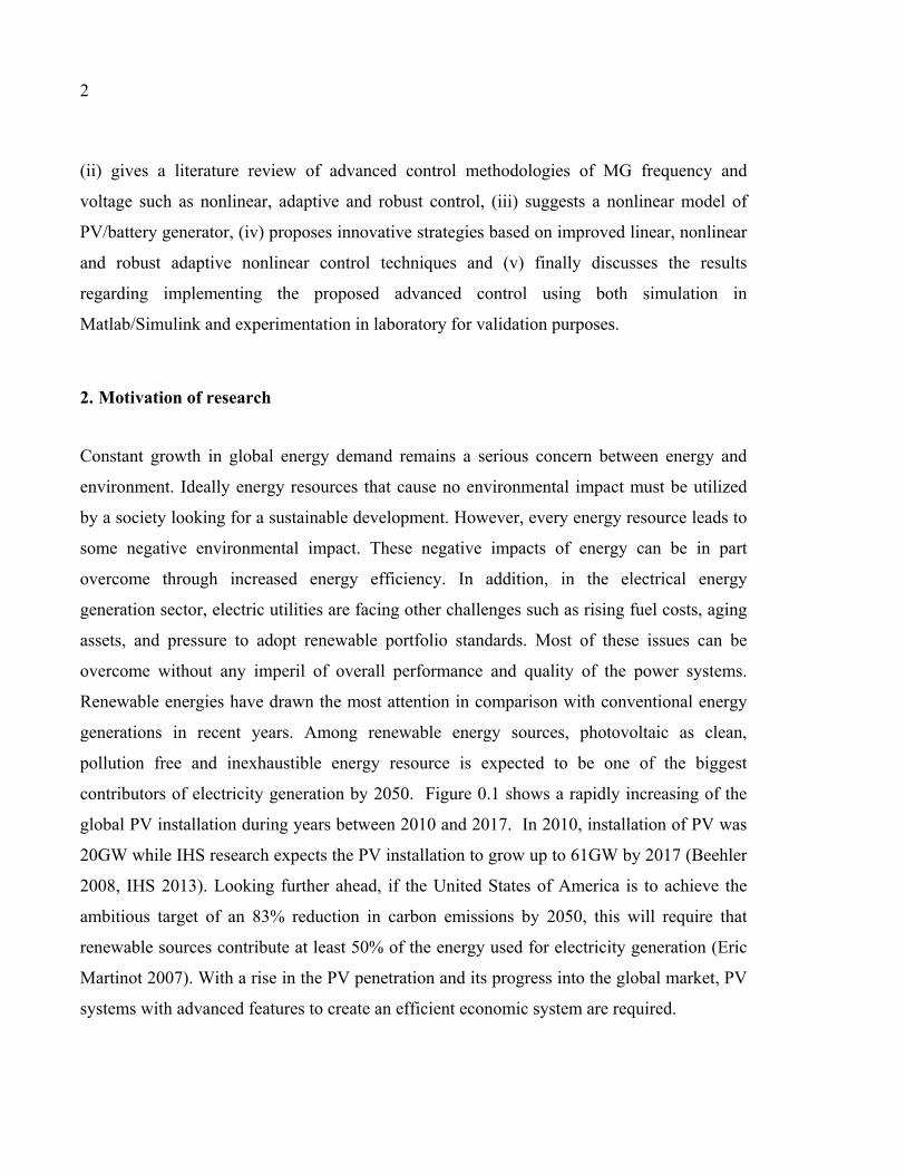
2. Motivation of research
Constant growth in global energy demand remains a serious concern between energy and
environment. Ideally energy resources that cause no environmental impact must be utilized
by a society looking for a sustainable development. However, every energy resource leads to
some negative environmental impact. These negative impacts of energy can be in part
overcome through increased energy efficiency. In addition, in the electrical energy
generation sector, electric utilities are facing other challenges such as rising fuel costs, aging
assets, and pressure to adopt renewable portfolio standards. Most of these issues can be
overcome without any imperil of overall performance and quality of the power systems.
Renewable energies have drawn the most attention in comparison with conventional energy
generations in recent years. Among renewable energy sources, photovoltaic as clean,
pollution free and inexhaustible energy resource is expected to be one of the biggest
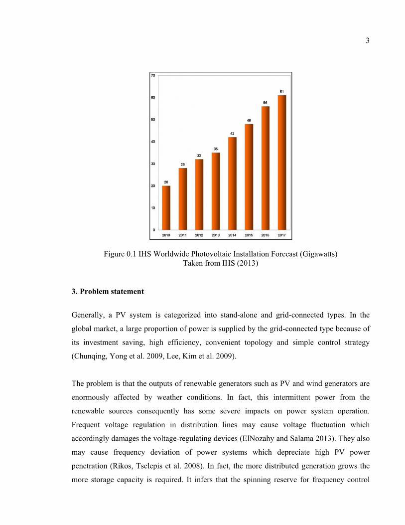
contributors of electricity generation by 2050. Figure 0.1 shows a rapidly increasing of the
global PV installation during years between 2010 and 2017. In 2010, installation of PV was
20GW while IHS research expects the PV installation to grow up to 61GW by 2017 (Beehler
2008, IHS 2013). Looking further ahead, if the United States of America is to achieve the
ambitious target of an 83% reduction in carbon emissions by 2050, this will require that
renewable sources contribute at least 50% of the energy used for electricity generation (Eric
Martinot 2007). With a rise in the PV penetration and its progress into the global market, PV
systems with advanced features to create an efficient economic system are required.
3
Figure 0.1 IHS Worldwide Photovoltaic Installation Forecast (Gigawatts) Taken from IHS (2013)
3. Problem statement
Generally, a PV system is categorized into stand-alone and grid-connected types. In the
global market, a large proportion of power is supplied by the grid-connected type because of
its investment saving, high efficiency, convenient topology and simple control strategy
(Chunqing, Yong et al. 2009, Lee, Kim et al. 2009).
The problem is that the outputs of renewable generators such as PV and wind generators are
enormously affected by weather conditions. In fact, this intermittent power from the
renewable sources consequently has some severe impacts on power system operation.
Frequent voltage regulation in distribution lines may cause voltage fluctuation which
accordingly damages the voltage-regulating devices (ElNozahy and Salama 2013). They also
may cause frequency deviation of power systems which depreciate high PV power
penetration (Rikos, Tselepis et al. 2008). In fact, the more distributed generation grows the
more storage capacity is required. It infers that the spinning reserve for frequency control

4
also decreases. If renewable energies are to provide a huge amount of microgrid power, they
will need to maintain some power in reserve. On the other hand, the sunlight or wind is not
always present or predictable. Therefore, a consideration of energy reserve facilities
supplementing a virtual spinning reserve seems to be one of the challenges of providing
frequency responsiveness and dispatchability to PV or wind systems. In fact, they store
power during normal operation and inject power during a fault, to maintain the proper micro
grid frequency and voltage. These storage facilities are newly deployed as distributed energy
storage (DES). However, they require extra cost and the sophisticated energy management is
necessary (Kakimoto, Takayama et al. 2009, Sow, Akhrif et al. 2011,Watson and Kimball
2011).
Another important challenge of current PV systems is that they are not well designed to
participate in the frequency regulation of the microgrid when it is affected by large
disturbances. Indeed, in conventional power systems, each synchronous generator (SG) could
respond to the frequency deviation because of the kinetic energy stored in rotor. However,
PV generator doesn’t have this rotating part to provide spinning reserve for frequency
regulation. Moreover, the typical concept of maximum power point tracking (MPPT)
conflicts with frequency regulation. Unlike the power deloading concept in conventional
power system, the MPPT algorithm doesn’t leave any power reserve to compensate the
frequency deviation. This results in a significant reduction of the robustness and frequency
regulation capabilities under higher PV penetration into microgrid system. As a consequence,
the frequency may change abruptly due to disturbances and parameters uncertainties in
generation or loads. Therefore, new trends of PV systems in a microgrid require being
equipped with an advanced and robust control unit which is able to contribute not only to
voltage but to frequency regulation as well (Yan, Jianhui et al. 2011). To be able to achieve
high performance renewable sources interacting appropriately with traditional micro power
grids, PV systems require reacting like conventional generators, such as synchronous
generator. Power network needs these types of renewable generators to support both voltage
and frequency regulation. To simultaneously support renewable generators with MPP

5
tracking and frequency regulating, PV systems should operate in conjunction with storage
components to have some power in reserve.
Considering storage devices in parallel with PV systems in a microgrid, the concepts of
energy management become necessary. Intelligent mechanisms are required to make PV and
microgrid interact properly. On the other hand, control techniques used in conventional PV
systems are mainly linear. However, to have PV and storage elements working together,
sophisticated switching power electronics devices are required. In the case when the
application calls for less power losses or large power transfer, it is necessary to use different
types of converters with more power electronics switches. Since the aforementioned system
(hybrid PV-battery generator) has severe nonlinear behavior, the use of a simple linear
controller is not adequate for such applications and doesn’t provide good performances.
4. Objectives of research
The main objective of this research is to make the PV-battery system behave like a
conventional generator e.g. synchronous generator while automatically managing power
sharing between different modules using an advanced and innovative control strategy. This
minimizes the costs and problems associated with the presence of rotating machines. On the
other hand the generated power (active or reactive) by PV-battery system increases when
both the MG frequency and voltage decrease respectively due to load demand increment, and
vice versa.
Specifically, this research aims to:
• ensure high performance voltage and frequency regulation in the presence of
fluctuations and load variations (Objective.1);
• integrate a conventional MPPT to ensure the PV operates at its maximum power point
(Objective.2);
• coordinate the power delivery among different units i.e. PV and battery system in a
MG without the need for a separate energy management system (Objective.3).

6
The overall expected configuration of the microgrid system associated with above-mentioned
objectives is presented in Figure 0.2.
2S
infL
Figure 0.2 Suggested microgrid system
5. Methodology
To achieve the objectives stated in previous section, this study is structured based on
modeling, control design and validation using both simulation and experimental investigation
at GREPCI laboratory. The proposed methodology is briefly described below:
First, in order to integrate photovoltaic, battery, synchronous generator using corresponding
power electronics converters and isolation transformers into a microgrid and to design a
unified controller for this system, a detailed model of the system is required. Hence an
accurate and nonlinear multi-input multi-output (MIMO) dynamical model of system is
extracted based on mathematical relationship among physical components. This model is
used for the design of an advanced control scheme i.e. robust adaptive nonlinear control.
Second, an advanced and innovative voltage and frequency control strategy which is robust,
adaptive and nonlinear is proposed via nonlinear dynamics of system. These controllers are
designed to drive switching converters such that the perturbation, uncertainty and

7
nonlinearity of the system as well as power sharing by battery are taken into account in
control design. To extract the optimum power of PV generator, a maximum power point
tracking (MPPT) algorithm is integrated into the controller.
Finally, validations of the proposed strategy are respectively conducted in two steps;
simulation and laboratory experimentation. To implement the proposed control methods, a
simulation model (see Figure 0.2) of the proposed system is developed in Matlab/Simulink
software. This includes modeling of controllers, PV array, power electronics converters,
lead-acid battery, transformer, load and synchronous generator. Some test methods are
applied to the simulation model to validate the control performance such as sun insolation
variation and load changes. Then, a hardware test bench is developed to verify the
effectiveness of control method. This experimental setup includes a PV array emulator, lead-
acid battery, synchronous generator, induction motor (IM) developed by Lab-Volt, drive
system with speed controller developed by ABB, three-phase transformer, DC-DC converter,
three-phase inverter and load. The developed control scheme is programmed and
implemented using Texas Instrument TMS320F28335 microcontroller. In fact, the C code
generated from the proposed controller through Simulink will be downloaded to the
microcontroller board, where it is executed in real time. The system is tested under different
scenarios in order to ensure the effectiveness of the proposed control methods such as
insolation and load changes.
6. Statement of the originality of the thesis
The lack of a systematic strategy for maintaining the voltage and frequency of microgrid when
PV system largely will be used has motivated the present study, which aims at developing an 8th
order dynamical model of the proposed PV-battery system (the first contribution). The
novelty of this model is the integration of the nonlinear dynamics of the microgrid frequency,
delivering powers and voltages. Using this comprehensive state variables representation, the
second contribution of this thesis is the design of unified multivariable controllers based on
techniques such as an improved linear, a nonlinear (an exact input-output feedback

8
linearization scheme) and a robust adaptive nonlinear control for the hybrid photovoltaic-
battery source in a MG system. These unique controllers (i) guarantee proper voltage and
frequency regulation in the presence of uncertainties, nonlinearities and disturbances (Saito,
Niimura et al.), (ii) integrate a conventional MPPT to ensure the PV operates at its maximum
power point and (iii) coordinate the power sharing among different units of the PV-battery
system.
7. Structure of the thesis
This thesis discusses major topics dealing with contribution of the PV system into the
frequency and voltage regulation of the microgrid system, as follows:
Chapter 1 is dedicated to the review of the recent approaches used for modeling, control and
implementation of microgrid with discussion on their specialties and abilities.
Chapter 2 describes thoroughly the full mathematical modeling of the selected configuration
of PV-battery generator in a MG.
Chapter 3 presents the design of the modified linear control for frequency and voltage
regulation in a microgrid including PV, battery system as well as synchronous generator. The
method is validated using simulation.
Chapter 4 proposes the design of a nonlinear control, based on exact input-output feedback
linearization for frequency and voltage regulation of a hybrid PV-battery system in parallel
with synchronous generator. The proposed nonlinear control is validated using both
simulation and laboratory experimentation.
Chapter 5 presents the design of a robust adaptive nonlinear control for frequency and
voltage support by a hybrid PV-battery system in parallel with synchronous generator. The
simulation result is included for validation of the proposed system.

9
Chapter 6 gives the general conclusions of this work and also highlights several
recommendations for future researches.

10

CHAPTER 1
LITERATURE REVIEW
1.1 Introduction
A literature review pertinent to recent methods on the performance of microgrid and its
control systems in the presence of renewable energy (RE) generators, in particular,
photovoltaic systems are presented in this chapter. Strengths, weaknesses as well as existing
challenges of state-of-the-art methods, categorized into the following four general subjects,
are well addressed.
First, different types of MG models suggested in literature including linear and nonlinear
models are presented. Second, various methods of classical and modern controls with the
contribution of photovoltaic generator into frequency and voltage regulation of the MG are
described. Third, several conventional maximum power point tracking (MPPT) methods,
used to harvest maximum energy from photovoltaic systems, are presented. Last, a set of
experimental testbeds of the MG energized by RE resources is discussed.
1.2 Overview of Microgrid Modeling
Different mathematical models have been so far suggested by researchers for a microgrid
system with various components consisting of power electronics converters, storage devices,
renewable energy sources, conventional generators and loads. The microgrid modeling
changes from one structure to another on the basis of used components. This section reviews
the main models which have been presented to date under the structure of both linear and
nonlinear models.
A first-order transfer function of each microsource in a microgrid consisting of photovoltaic
system, wind turbine, fuel cell, diesel engine generator, battery and flywheel storage system
is suggested in (Senjyu, Nakaji et al. 2005) as:

12
= 1 + (1.1)
where G, T and K represent respectively the transfer function, the time constant and the
transfer function gain of the model of each generator. This method introduces a simple
approximation of microgrid model commonly for large-scale system and its power flow
analysis. The weakness of this method is that the exact dynamics of the system such as power
converter modeling are not considered. In other words this model doesn’t represent the real
behavior of MG to be used for control design. To address this drawback, a bunch of
researches have focused on dynamic modeling of microgird. For example in (Berridge 2010,
Karimi, Davison et al. 2010, Bidram, Davoudi et al. 2013), a microgrid structure, consisting
of a single DC source connected to a voltage-source converter (VSC) with inductive L filter
and passive RLC load, is selected as illustrated in Figure 1.1.
Figure 1.1 Microgrid model Taken from Karimi, Davison et al. (2010)
In these works, the dynamics of MG illustrated in Figure 1.1 is modeled by a nonlinear
equation in d-q (direct-quadrature) frame to obtain the standard state space model. The high
switching frequency harmonics, considered as disturbance signals, are added to the non-
polluted input control signals.

13
The idea of representing microgrid with a DC source is extended for two generators
interfaced in parallel while the passive load is connected at point of common coupling (PCC)
(Marwali and Keyhani 2004, Moradi, Karimi et al. 2010, Babazadeh and Karimi 2011). The
configuration of this MG is illustrated in Figure 1.2. The nonlinear dynamical equations of
microgrid are then obtained by applying Kirchhoffs Voltage Law (KVL) and
Kirchhoffs Current Law (KCL) in dq-frame. These models are used for designing the
decentralized control where each generator is equipped with a separate controller. In these
two previous methods, distributed generators dynamics are neglected by a DC source for the
sake of simplicity. Since the dynamics of DGs affect the system performance especially for
control design, other studies choose a complete configuration as shown in Figure 1.3.
Figure 1.2 The microgrid structure with two generators in parallel Taken from Babazadeh and Karimi (2011)
The microgrid architecture in (Pogaku, Prodanovic et al. 2007, Nejati, Nobakhti et al. 2013)
includes the model of distributed generators such as photovoltaic array, fuel cell and micro-
turbine i.e. synchronous generator in addition to the converter models.

14
Figure 1.3 Configuration of a complete microgrid system Taken from Pogaku, Prodanovic et al. (2007)
In recent years, the contribution of the renewable energy-based generators as of conventional
generators to frequency support of a microgrid has taken some attention. Therefore a
complete microgrid model including the frequency model supported by renewable energy
generators is of interest. In (Sow, Akhrif et al. 2011) authors suggested a nonlinear model of
DFIG-based wind generator to contribute to the primary and secondary frequency support of
MG. In this work, the rotor speed dynamics are added to the dynamics of inverter to increase
inertia of the system. Authors consider a transformer for connecting the DFIG to high voltage
system, while the dynamics of transformer and its parameters such as leakage inductance are
neglected in the model. The model in this work is limited to a very specific application of
wind generator. For other types of RE generators with no rotating part such as photovoltaic
arrays, this model is not effective.
Authors in (Okou, Akhrif et al. 2012) suggest a general frequency dynamics for PV
application independent of the speed dynamics. In fact the inertia is added by deloading the
PV power. The drawback of this approach is that it adds some unknown parameters, such as
the equivalent droop coefficient of power system and the time constant, to the MG model.
Therefore it needs a modern controller to compensate the uncertainties. In addition there
remains a trade-off in meeting both requirements of the MPPT and frequency regulation due
to the lack of an actual storage system.
15
The most recent researches addressed this problem by suggesting Synchroconverters, i.e.,
inverters that mimic synchronous generators (Zhong 2010, Qing-Chang and Weiss 2011,
Qing-Chang, Phi-Long et al. 2014). This model of inverter behaving like a synchronous
generator can be used in a traditional power system where a significant proportion of the
generation is inverter-based. Similar to the previous method, the model poses several
unknown parameters which authors leave the methodology of choosing these parameters and
their impact on real power system as a future work. Therefore, this model remains a
challenge for control design engineers.
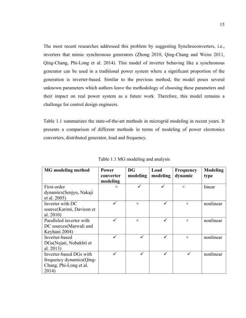
Table 1.1 summarizes the state-of-the-art methods in microgrid modeling in recent years. It
presents a comparison of different methods in terms of modeling of power electronics
converters, distributed generator, load and frequency.
Table 1.1 MG modeling and analysis
MG modeling method Power converter modeling
DG modeling
Load modeling
Frequency dynamic
Modeling type
First-order dynamics(Senjyu, Nakaji et al. 2005)
× × linear
Inverter with DC source(Karimi, Davison et al. 2010)
× × nonlinear
Paralleled inverter with DC sources(Marwali and Keyhani 2004)
× × nonlinear
Inverter-based DGs(Nejati, Nobakhti et al. 2013)
× nonlinear
Inverter-based DGs with frequency dynamics(Qing-Chang, Phi-Long et al. 2014)
nonlinear

16
1.3 Overview of MG Control methods
Microgrid control can be classified into three layers as of the primary, secondary and tertiary
control (De Brabandere, Vanthournout et al. 2007). The primary layer or field level, which is
the main concentration of this thesis, is principally performed on a local control of power
converters ensuring frequency and voltage regulation based on the reference signals received.
On this layer there is no communication among devices. The secondary layer (Katiraei,
Iravani et al. 2008) is responsible for modifying the commanded signals (desired frequency
and voltage) to be sent to the primary level control, according to the grid synchronization
(via phase locked loop PLL), frequency and voltage restoration techniques. The tertiary
control is responsible for dispatching power on the basis of economic and availability of the
generators in distribution network operation. On the other hand, the tertiary control task is the
management of the importation or exportation of active and reactive power to or from the
grid by sending reference signals to the secondary control (Vasquez, Guerrero et al. 2010,
Mohamed and Radwan 2011). Figure 1.4 demonstrates the architecture of a typical microgrid
control.
Figure 1.4 A typical microgrid control architecture Taken from Vasquez, Guerrero et al. (2010)

17
Since this PhD work concentrates on MG islanded mode operation, recent primary control
approaches in a microgrid with participation of renewable energy generators (i.e.
photovoltaic (PV) generator) including frequency and voltage regulation along with MPPT
methods are mainly presented in this section.
Frequency and voltage control strategies: A primary control level
In autonomous (islanded) mode, where the microgrid system is not supported by the
robustness of the main grid, several works have been carried out on MGs’ frequency and
voltage control in recent years. These controllers are categorized into two groups: classical
and modern control approaches which are presented as follow.
A. Classical control
The conventional techniques of the voltage and frequency control without the presence of
communication protocols are based on droop controls (Chandrokar, Divan et al. 1994, Piagi
and Lasseter 2006, Barklund, Pogaku et al. 2008, De and Ramanarayanan 2010). The
conventional droop control of MG is based on mimicking the Synchronous Generator (SG)
operation. In conventional generator like SG, the measured power, P, is changed by droop
control as a function of frequency, P(f). When the output ac power is larger than input
mechanical power of SG, the generator slows down due to its inertia. As a consequence, the
frequency (and on the other hand the phase angle) at SG terminal lowers. In fact, inverter
based MG lacks the inertia. The droop controls in these types of MGs are based on the line
characteristics.
The droop control technique in MGs avoids the requirement of complex and costly
supervisory system. In addition, the plug-and-play feature of each unit makes the expansion
of these systems easier. However, the droop controls have shown some drawbacks such as
dependencies on inverters output impedance and trade-off between the accuracy of power
sharing and voltage/frequency deviation (with respect to nominal set-points). Some following

18
modifications of the droop control based on the line characteristics and power flow between
buses have been proposed to lessen the effect of these problems. Active and reactive powers
(P and Q respectively) flowing between sources ∢ and ∢ with the line impedance
Z=R+jX are calculated as (Yun Wei and Ching-Nan 2009):
= + [ ( − cos( − )) + sin( − )] = + [− sin( − )) + ( − cos( − ))]
(1.2)
For inductive line impedance with negligible relative phase angle (i.e. = 0, ( − )
small) the above equations are simplified to,
≈ [ ( − )] ≈ [ − ]
(1.3)
Therefore, for inductive network the active and reactive power values are controlled directly
by the phase angle and the voltage amplitude respectively. Due to a linear relationship
between the angle and the frequency, the frequency is used in control purposes for the sake
of simplicity (Phadke, Thorp et al. 1983). Therefore, the generator power is controlled by
measured frequency (P(f)). Unlike in SGs where the frequency depends on the rotating
speed, in inverter-based MG the frequency is controlled independently. In addition, the
power measurement is easier than the instantaneous frequency measurement in microgrid
(Arboleya, Diaz et al. 2010). Therefore the drop of frequency as a function of active power is
proposed f(P)
= − ( − ) (1.4)

19
where , , and represent the actual and reference of frequency as well as active power
respectively. The coefficient is the slope of the frequency droop characteristics. Figure 1.5
shows typical droop characteristics.
Figure 1.5 p-f droop characteristics
Similarly, the voltage amplitude of microgrid terminal is controlled by reactive power such
that,
= − ( − ) (1.5)
where , , and represent the actual and reference of voltage amplitude as well as
reactive power. The coefficient is the positive droop gain. Figure 1.6 illustrates the
configuration of the traditional droop control methods based on Q-v and P-f for two VSCs
with sharing a common load.

20
Figure 1.6 Traditional P-F and Q-V droop control methods for microgrid Taken from Hu, Kuo et al. (2011)
In fact, the droop gain is chosen such that to compromise between high gain which causes
system instability due to the big frequency/voltage drop in steady state regime and low value
gain which increases the settling time. Moreover big load change can vary the
frequency/voltage far from its nominal value which reduces the MG stability or even makes
it unstable. This approach poses a steady state frequency/voltage drop with respect to load
changes (Guerrero, Matas et al. 2006, Guerrero, Vasquez et al. 2011). Despite the droop
control being a decentralized control approach, the autonomous power sharing of output
power converters are highly dependent on the inverter output impedances (Tuladhar, Hua et
al. 2000). These impedances are unknown or vary from each design to another (Lee, Chu et
al. 2013). A slow dynamic response of system with conventional droop control is obtained
due to the low pass filter which is used for the calculation of average active and reactive
powers.

21
To remove the static error and to reduce the dependency of the conventional droop on the
load changes, the integral term is added in previous works (Katiraei and Iravani 2006, Lee
and Wang 2008, Haruni, Gargoom et al. 2010, Ray, Mohanty et al. 2010, Jayalakshmi and
Gaonkar 2011, Kasal and Singh 2011) as,
= + ( − ) + , ( − ) (1.6)
= + ( − ) + , ( − ) (1.7)
in which, the parameters , and , are the coefficients of the integral terms. To improve
the transient response of the system, a derivative term is added to the conventional droop
control as, (Goya, Omine et al. 2011).
= + ( − ) + , (1.8)
= + ( − ) + , (1.9)
where the parameters , and , are the coefficients of the derivative terms.This method is
effective for a small microgrid with large load change through avoiding large start-up
transience (Mohamed and El-Saadany 2008). However, the high derivative gain causes noise
amplification in control system. One common approach is to use a washout filter which is in
fact a high pass filter ( ) with time constant and derivative gain . Although
washout filters have been successfully used in many control applications, there is no
systematic way to choose the constants of the washout filters and the control parameters
(Hassouneh, Lee et al. 2004). This causes a trade-off between high frequency attenuation (a
satisfactory damping using ) and the error of the fundamental components ( , high
enough allowing the input signals to pass) (Farahani 2012).

22
Another problem facing the conventional droop control is the active and reactive power (P-
Q) coupling. To overcome this problem a method based on virtual output inductance is
proposed.
According to Equation (1.3), to have a decoupled droop characteristics, line impedance
should be inductive. Therefore, on the control design stage, a virtual inductor is included at
the inverter output without the information of line impedance (Funato, Kamiyama et al. 2000,
Dranga, Funato et al. 2004). The reference voltage in voltage controller of Equation (1.9) is
modified as,
= − (1.10)
where , , , and are the reference and modified reference voltage of the droop
control, virtual inductance and line inverter current. Although this method is effective in
decoupling the active and reactive powers (He and Li 2011, Cheng, Li et al. 2012, Savaghebi,
Jalilian et al. 2012), it causes high frequency noise amplification due to the derivative term as
well as reactive power sharing error due to the increased voltage drop as shown in Equation
(1.10). In (Yun Wei and Ching-Nan 2009), the reactive power control is enhanced by the
estimation of the inductor voltage drop as well as the load estimation. Droop control with
virtual inductor control is shown in Figure 1.7.
Figure 1.7 Droop control with virtual inductor control Taken from Cheng, Li et al. (2012)
23
The previous methods are essentially devoted to the high voltage application of microgrid. In
traditional power system with high voltage (Holland, Kirschvink et al.) transmission line
where ≫ , the voltage is directly controlled by reactive power and frequency is controlled
by active power (conventional P-f and Q-v droop control). However, in low voltage (Vallvé,
Graillot et al.) microgrid where the feeder impedance is not inductive, the line resistance
should not be neglected (Laaksonen, Saari et al. 2005), because ≫ . In case of resistive
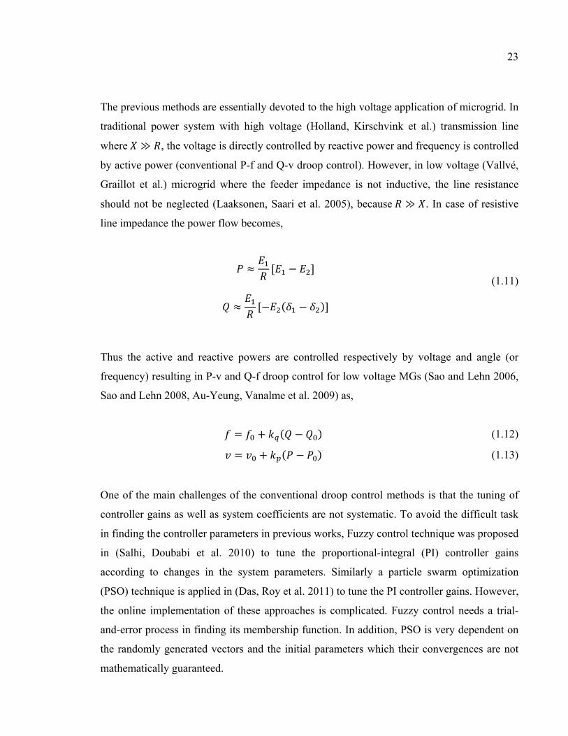
line impedance the power flow becomes,
≈ [ − ] ≈ [− ( − )]
(1.11)
Thus the active and reactive powers are controlled respectively by voltage and angle (or
frequency) resulting in P-v and Q-f droop control for low voltage MGs (Sao and Lehn 2006,
Sao and Lehn 2008, Au-Yeung, Vanalme et al. 2009) as,
= + ( − ) (1.12) = + ( − ) (1.13)
One of the main challenges of the conventional droop control methods is that the tuning of
controller gains as well as system coefficients are not systematic. To avoid the difficult task
in finding the controller parameters in previous works, Fuzzy control technique was proposed
in (Salhi, Doubabi et al. 2010) to tune the proportional-integral (PI) controller gains
according to changes in the system parameters. Similarly a particle swarm optimization
(PSO) technique is applied in (Das, Roy et al. 2011) to tune the PI controller gains. However,
the online implementation of these approaches is complicated. Fuzzy control needs a trial-
and-error process in finding its membership function. In addition, PSO is very dependent on
the randomly generated vectors and the initial parameters which their convergences are not
mathematically guaranteed.

24
In addition to the droop control methods, some other researchers suggest different techniques
based on deloading power and virtual inertia for the inverter-type microgrid system
(Kakimoto, Takayama et al. 2009, Das, Roy et al. 2011). A control method based on simple
fuzzy logic was proposed in (Datta, Senjyu et al. 2011) for the PV–diesel hybrid system to
introduce the frequency control by the PV and to produce the output power command. Three
inputs-frequency deviation (from frequency reference) of the isolated utility, average
insolation, and change of insolation- are considered for fuzzy control. A control method
based on a load power estimator and an energy storage system is proposed for isolated
photovoltaic–diesel hybrid system to provide frequency control. In this method, photovoltaic
power is controlled according to the load variation to minimize the frequency deviations.
Load power is estimated by a minimal-order observer. Then, a load variation index is
calculated. A base photovoltaic power, produced from the available maximum photovoltaic
power using a low-pass filter, is added to the load variation index to generate the command
photovoltaic power. Since the voltage source inverter along with renewable energy sources
(such as PV array generators) are inertia-less, this method of deloading enhances the inertia
of the MG system. The weakness of this method is that the maximum power of PV is not
always available. On the other hand, PV generator permanently operates below the optimal
power to provide a reserve under load power disturbance in order to participate to frequency
regulation. The low pass filter used in this design which slows down the system dynamic
response is another drawback of this technique.
To increase the inertia and avoid the confliction of frequency and MPPT mentioned in
previous publications, frequency regulation in an island and weak power system using large
battery energy storage is discussed in (Kottick, Blau et al. 1993). The sole purpose of
frequency control is dependent on the battery. In (Li, Song et al. 2008), frequency control
was applied to a microgrid consisting of hybrid fuel-cell/wind/PV system. Required power of
the electrolyser system is supplied mainly by the wind and PV, and the hydrogen produced
by the electrolyser system is stored in the hydrogen tank to be converted back to electricity in
the fuel cells. This mechanism emulates storage for the MG system to increase the inertia.

25
In addition to frequency participation through renewable generator, PV inverters which
provide the reactive power to support voltage control have drawn more attention in recent
years (Farivar, Clarke et al. 2011, Jahangiri and Aliprantis 2013,Robbins, Hadjicostis et al.
2013). However there are some drawbacks that prevent the PV inverters to support reactive
power in order to compensate the voltage. Based on the effective IEEE Std. 1547 the utilities
do not accept the PV inverter to inject the reactive power. This conflicts with the unity power
factor inverter although the new IEEE standards try to lessen some of these constraints
(Basso and DeBlasio 2004). In addition, more expensive oversized inverter reduces the profit
of the PV inverter owner. Moreover, the coordination between this type of PV inverter and
other traditional inverters is reduced.
In conclusion to the classical control techniques in microgrid design, these model-free
control works do not explicitly take into account the nonlinear behavior of MG systems
incorporating renewable energy sources and power electronic interfaces. In addition, these
linear controllers are not designed to perform uniformly over a wide range of operating
conditions or in the presence of nonlinearities, uncertainties and disturbances. Moreover, the
different control modules are designed independently. The lack of coordination among the
disparate units makes it a difficult task to meet frequency and voltage regulation as well as
MPPT requirements. In most applications, a complex and often costly energy management
unit is needed. Table 1.2 which summarizes the traditional methods of frequency and voltage
control with their different features is presented below.

26
Table 1.2 Classical frequency and voltage control of microgrid
MG control method MPPT Frequency
control voltage control
P/Q decupling
application
Conventional P-f vs. Q-v droop control (Yun Wei and Ching-Nan 2009)
× HV MG
conventional droop with integral term (Ray, Mohanty et al. 2010)
× HV MG
conventional droop with derivative term (Goya, Omine et al. 2011)
× HV MG
conventional droop with virtual output inductor (Funato, Kamiyama et al. 2000)
× HV MG
conventional P-v and Q-f droop (Sao and Lehn 2006)
× LV MG
Conventional droop P-v with virtual output resistance (Guerrero, Matas et al. 2007)
× LV MG
Modified droop control with soft-computing techniques (Datta, Senjyu et al. 2011)
× HV or LV
MG
Power modulation and virtual inertia control for PV inverter with storage system (Li, Song et al. 2008)
HV or LV
MG
B. Modern control
Among existing modern control methods, those commonly used in power network such as
nonlinear control, adaptive nonlinear control and robust adaptive nonlinear control are
presented in this section.

27
i. Nonlinear control
Recently nonlinear control techniques such as sliding mode control, backstepping and input-
output feedback linearization have drawn interest in power electronics applications since they
offer systematic, powerful and easy-to-implement methods (Marino and Tomei 1996). A
nonlinear frequency and voltage control based on backstepping technique is developed for
PV generator in (Okou, Akhrif et al. 2012). A multi-input multi-output MIMO nonlinear
frequency and voltage control based on feedback linearization technique is developed for
doubly-fed induction generators (DFIG) generator connected to synchronous generator (Sow,
Akhrif et al. 2011). It is shown in these studies that the nonlinear control approach improves
the general system performance in both transient and steady-state regimes since the exact
nonlinearity of system is taken into account in control design. The lack of storage system in
both techniques causes the renewable generator to operate below its maximum power point,
MPP. The effectiveness of these nonlinear control approaches is highly dependent on the
system parameters. On the other hand uncertainties in parameters such as load power,
terminal voltage of SG, line inductance and SG, PV, DFIG model parameters affects the
controller tracking.
ii. Adaptive nonlinear control
The design of adaptive control was introduced in 1950s. The first and most important
applications of adaptive control were in mill industries in Sweden. Another important
application of adaptive control has been the design of autopilots in flight control. The
airplanes operate over a wide range of speeds and altitudes with nonlinear and time-varying
dynamics. The different operating conditions of aircraft lead to the different unknown
parameters in the system model. A sophisticated feedback control needs to be able to learn
about parameter uncertainties. Two adaptive approaches were introduced in the literature;
"direct and indirect" adaptive controls. In indirect adaptive control, the plant parameters are
estimated online and used to calculate the control parameters. In direct adaptive control, the
controller parameters are estimated directly without estimating the plant parameters (Krstic,
Kanellakopoulos et al. 1995, Kaufman, Barkana et al. 1998, Åström and Wittenmark 2013).

28
In a microgrid system with renewable energy integration, the system parameters change due
to the load perturbation or the fluctuation in the intermittent power of renewable generator.
Moreover there are some parameters in the system model which are unknown. An adaptive
control can improve the system performance by estimating the unknown parameters
(Yazdani, Bakhshai et al. 2008). Some applications of adaptive control within a microgrid in
recent years are listed as: the estimation of the grid frequency in a phase-locked loop (PLL)
for active power filtering (Hogan, Gonzalez-Espin et al. 2014), the regulation of the common
DC bus voltage with different renewable energy generators (Dragicevic, Guerrero et al.
2014), the adjustment of the weighted coefficients of active power-frequency droop (Li,
Wang et al. 2015), the load sharing in a parallel-connected DC-DC converters in a DC
microgrid (Augustine, Mishra et al. 2015), the protection and control (Laaksonen, Ishchenko
et al. 2014) and the power balance during transition from grid-connected to islanding mode
in a microgrid (Shi, Sharma et al. 2013). A nonlinear controller based on sliding mode
control with adaptive voltage droop was proposed for a microgrid (Ferreira, Barbosa et al.
2013). The advantage of the adaptive nonlinear control is that it improves system behavior
under both nonlinearities and uncertainties. To the best of our knowledge, no research has
addressed the adaptive nonlinear control of a microgrid integrated with photovoltaic
generators along with storage devices in the literature. Therefore it motivates us to
investigate this subject in the next chapters of this thesis.
iii. Robust adaptive nonlinear control
The adaptive laws and control discussed in previous section are designed with the
assumption that the plant model is free of noise and disturbance. The designed controller is to
be implemented on a practical system that is likely to differ from its mathematical and ideal
models. The actual plant can be corrupted by noising measurement or any external
disturbance. The discrepancies between the developed and real models may affect the system
performance and robustness.
29
The theory of robust adaptive nonlinear control was first presented by Kokotovic and Marino
in 1991 (Kanellakopoulos, Kokotovic et al. 1991). A new robust adaptive nonlinear control
based on backstepping scheme for frequency and voltage regulation was designed for DFIG
wind turbine (Okou and Amoussou 2008). This strategy takes into account the uncertainty,
disturbance and nonlinearity of the system in the control design. However the problems
associated with the microgrid lacking the storage system (i.e. MPPT vs. frequency
confliction) and inertia-less generators such as PV system (i.e. virtual inertia) are not
addressed.
Overview of the recent maximum power point tracking approaches
The low energy conversion efficiency of PV array hinders the widespread use of PV in
power systems. In order to overcome this drawback, maximum power should be extracted
from the PV system. This objective can be achieved by a MPPT which identifies the optimal
operation of the PV systems.
To date, several MPPT techniques have been reported which can be sorted into three
categories; namely the conventional, soft computing and advanced model-based methods.
Among conventional MPPT methods reported in the literature, the hill climbing (Elgendy,
Zahawi et al. 2011, Ahmed, Li et al. 2012, Kumar 2012, Abuzed, Foster et al. 2014), perturb
and observe (P&O) (Femia, Petrone et al. 2004, Liu and Lopes 2004, Femia, Petrone et al.
2005, Khaehintung, Wiangtong et al. 2006, Fangrui, Yong et al. 2008) and incremental
conductance (IC) (Yuansheng, Suxiang et al. 2012, Guan-Chyun, Hung et al. 2013, Latif and
Hussain 2014) are commonly used since they are quite simple to implement and they exhibit
a good convergence speed. However, the oscillation around the MPP is the major drawback
of theses algorithms (Banu, Beniuga et al. 2013). The oscillatory behaviour around the MPP
reduces considerably the system efficiency due to power losses. Moreover, when the
atmospheric condition varies, these methods may be confused since the operating point can
move away from the MPP instead of working around it. In order to minimize the oscillation,
several attempts were made by reducing the perturbation step size. However, a smaller

30
perturbation size affects the tracking speed adversely (Sera, Mathe et al. 2013, Shah and
Joshi 2013).
In order to improve the abovementioned drawback, soft computing (SC) techniques such as
fuzzy logic control (FLC) (Ze, Hongzhi et al. 2010, Chin, Tan et al. 2011, Ze, Hongzhi et al.
2011, Arulmurugan and Suthanthira Vanitha 2013, Roy, Basher et al. 2014), Artificial
Neural-Network (ANN) (Kaliamoorthy, Sekar et al. 2010, Phan Quoc, Le Dinh et al. 2010,
Pachauri and Chauhan 2014), genetic algorithm (Ramaprabha, Gothandaraman et al. 2011,
Daraban, Petreus et al. 2013, Hadji, Gaubert et al. 2014, Mohamed, Berzoy et al. 2014),
differential evolution (DE) (Taheri, Salam et al. 2010, Sheraz and Abido 2012, Taheri, Taheri
et al. 2012), particle swarm optimization (PSO) (Kondo, Phimmasone et al. 2010,
Phimmasone, Kondo et al. 2010) and firefly (FA) (Sundareswaran, Peddapati et al. 2014)
algorithms have attracted much interest over the past years. One of the distinctive features of
the soft-computing MPPT techniques comparing with other MPPT approaches is that they
outperform in global searching during partial shading condition in PV system. Despite of
their effectiveness, SC algorithms are more highly dependent on the complexity of
computing programs (Paul 2013). In FLC MPPT, the membership function is generated
through a time-consuming process. One of the major criticisms of ANN MPPTs is that they
are considered as black boxes. Therefore no satisfactory explanation of their behaviour is
offered. In stochastic techniques the decision variable, either the duty cycle of the power
electronic converter or the reference voltage of the controller, is employed by the random
vectors during the execution of algorithm. Therefore the global MPP convergence cannot be
mathematically guaranteed.
In order to overcome the problems of previous methods, in particular, the oscillatory
behaviour and complexity of existing MPPT algorithms, a new trend of MPPTs based on
model-based approaches has been suggested in very recent years. Sliding mode controller
MPPTs (SMC-MPPTs) (Siew-Chong, Lai et al. 2007, Siew-Chong, Lai et al. 2008, Yan Ping
and Fang Lin 2009, Pradhan and Subudhi 2015) possess robustness of tracking control and

31
stability against internal system parameters and load uncertainties. Adaptive MPPT based on
variable scaling factor has been suggested in using proposed small-signal model (Kui-Jun
and Rae-Young 2012, Kui-Jun and Rae-Young 2012). Robust adaptive sliding mode control
scheme has been developed for MPPT in (MacKunis, Reyhanoglu et al. 2012). Unlike the
MPPTs based on soft computing techniques such as DE, PSO, and FA MPPTs which
outperform under partial shading condition (the existence of the multiple peaks on PV
characteristics), the model-based MPPTs (i.e. nonlinear MPPT controller) suggested in the
literature are not ready for PV system exposed in partial shading condition. Therefore these
types of model-based MPPTs can be improved for global optimization. The comparison of
recent MPPTs is listed in the following table.
Table 1.3 Comparison of MPPTs in PV application
MPPT methods and Criteria
Conventional MPPTs
(P&O, IC, etc.)
Soft-computing MPPTs
(ANN, FLC, DE, PSO,
etc.)
Modern control
(adaptive, SMC,
nonlinear MPPTs)
Convergence in uniform condition
Yes Yes Yes
Convergence in partial shading condition
No Yes No
Design complexity simple complex moderate
Convergence speed vs. accuracy
very low high high
Dependency on initial parameters
moderate high moderate
1.4 Microgrid testbeds
This section lists the recent development in the industrial and academic microgrid testbeds
and example cases as of either remote MG or utility MG supplied by both diesel and
renewable DGs for different applications such as military, remote area, uninterruptable
power supply, emergency power, electric vehicle and residential application.

32
Boston Bar – British Columbia (BC) Hydro, Canada:
Boston Bar substation is connected to BC Hydro grid through a 60Km, 69KV transmission
line and a 14MVA transformer. This traditional transmission faces frequent blackouts due to
climate conditions. To provide improved reliability on rural feeders, a microgrid with three
feeders has been interconnected to the 69KV by a 69KV/25KV substation since 1995. The
MG includes two hydropower generators 8.75 MVA, 0.8pf. Although no physical storage
system is considered in the design of microgrid, the inertia of generators is enlarged (Peralta,
Iosfin et al. 2009). Figure 1.8 demonstrates the configuration of the Boston Bar microgrid.
Figure 1.8 The Boston Bar BC hydro microgrid Taken from Katiraei, Abbey et al. (2008)
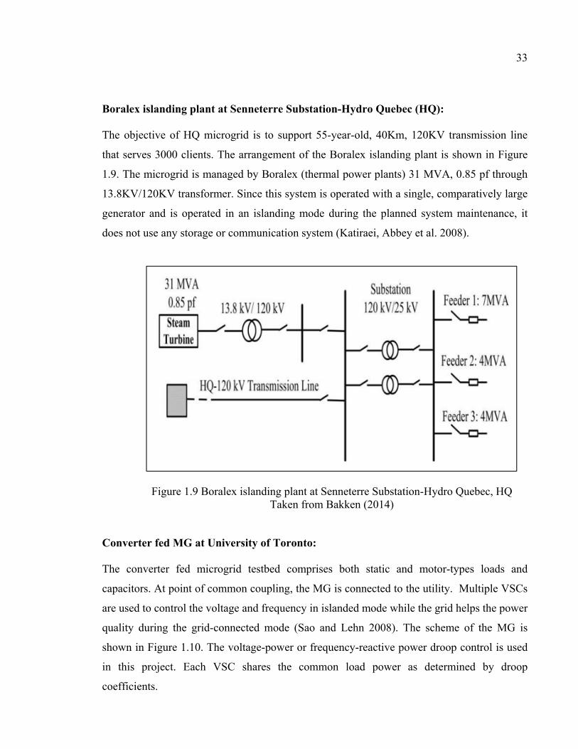
33
Boralex islanding plant at Senneterre Substation-Hydro Quebec (HQ):
The objective of HQ microgrid is to support 55-year-old, 40Km, 120KV transmission line
that serves 3000 clients. The arrangement of the Boralex islanding plant is shown in Figure
1.9. The microgrid is managed by Boralex (thermal power plants) 31 MVA, 0.85 pf through
13.8KV/120KV transformer. Since this system is operated with a single, comparatively large
generator and is operated in an islanding mode during the planned system maintenance, it
does not use any storage or communication system (Katiraei, Abbey et al. 2008).
Figure 1.9 Boralex islanding plant at Senneterre Substation-Hydro Quebec, HQ Taken from Bakken (2014)
Converter fed MG at University of Toronto:
The converter fed microgrid testbed comprises both static and motor-types loads and
capacitors. At point of common coupling, the MG is connected to the utility. Multiple VSCs
are used to control the voltage and frequency in islanded mode while the grid helps the power
quality during the grid-connected mode (Sao and Lehn 2008). The scheme of the MG is
shown in Figure 1.10. The voltage-power or frequency-reactive power droop control is used
in this project. Each VSC shares the common load power as determined by droop
coefficients.

34
Figure 1.10 Converter fed MG at Toronto Taken from Sao and Lehn (2006)
Microgrid testbed at Rochester Institute of Technology (RIT) New York:
This testbed integrates energy production and storage resources within a single
microgrid. The microgrid testbed has several units including wind turbines, solar panels,
400KW fuel cells, 50KWh battery bank, geothermal heating/cooling system with intelligent
energy tracking system and research data center as illustrated in Figure 1.11. The power
generated by RIT microgrid is used for vehicle charging station, building lighting and electric
outlets (RIT, 2015).
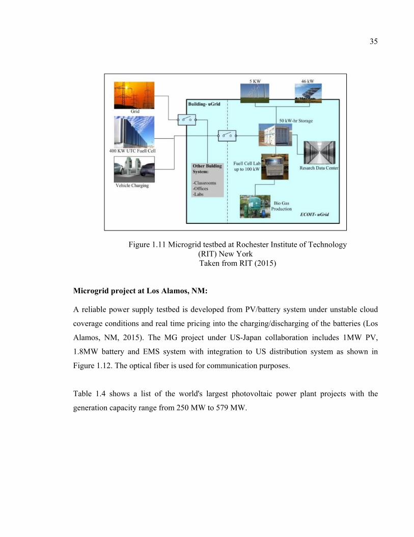
35
Figure 1.11 Microgrid testbed at Rochester Institute of Technology (RIT) New York Taken from RIT (2015)
Microgrid project at Los Alamos, NM:
A reliable power supply testbed is developed from PV/battery system under unstable cloud
coverage conditions and real time pricing into the charging/discharging of the batteries (Los
Alamos, NM, 2015). The MG project under US-Japan collaboration includes 1MW PV,
1.8MW battery and EMS system with integration to US distribution system as shown in
Figure 1.12. The optical fiber is used for communication purposes.
Table 1.4 shows a list of the world's largest photovoltaic power plant projects with the
generation capacity range from 250 MW to 579 MW.

36
Figure 1.12 Microgrid project at Los Alamos, NM Taken from Los Alamos, NM, (2015)
Table 1.4 The world's largest photovoltaic power plant projects
Taken from Dara Jegede (2017)
Photovoltaic power plant projects Country Generation
capacity
Solar Star Projects, California USA 579MW
Desert Sunlight Solar Farm, California USA 550MW
Topaz Solar Farms, California USA 550MW Longyangxia Dam Solar Park, Qinghai China 530 MW Golmud Solar park, Qinghai China 500MW Copper Mountain Solar Facility, Nevada USA 458 MW Charanka Solar Park, Gujurat India 345MW Cestas Solar Farm, Bordeaux France 300 MW Agua Caliente Solar, Arizona USA 290MW California Valley Solar Ranch (CVSR) in San Luis Obispo USA 250MW

CHAPTER 2
MATHEMATICAL MODELING
2.1 Introduction
This chapter presents a number of models associated with the microgrid elements, developed
at GREPCI laboratory during this Ph.D. project. As sketched in Figure 2.1, the model
comprises a PV/battery generator consisting of a photovoltaic array in series with a DC-DC
boost converter, a storage device in series with a bidirectional DC-DC boost converter, a
three-phase DC-AC inverter, smoothing inductors and a step-up transformer. The secondary
of the transformer is connected to an AC load and a synchronous generator (SG) via a
transmission line. This chapter is structured in two general sections as follows: a commonly
used model of a PV system (i.e. PV cell/module/array), power electronic converters (i.e.
modulation techniques, steady-state and dynamic analysis), synchronous generator (i.e.
voltage vs. speed control, the transient and saturated model and swing equation) and
frequency model is described. The model includes a novel nonlinear dynamical model (of 8th
order) of the PV/battery generator along with power conditioning system. This model will be
used for the design of advanced control schemes such as the nonlinear and robust adaptive
nonlinear controllers in next chapters.
2S
Mot
orinfL
Figure 2.1 Microgrid system

38
2.2 Photovoltaic (Cell/module/array) model
2.2.1. Solar cells
Solar cells are constructed by semiconductor materials (e.g. silicones) which form an electric
field positive on backside and negative towards the sun. In the dark, the solar cell treats as a
diode device. If it is connected to an external voltage source, it generates a current DI which
is named diode or dark current. When exposed to the light, photons (solar energy) are
absorbed by the semiconductors and create a current phI
proportional to the incident
irradiance (Lorenzo 1994). Figure 2.2 depicts one of the more commonly used solar cell
equivalent circuit models (Liu and Dougal 2002).
Figure 2.2 PV cell equivalent circuit
This circuit simplifies the PV cell by a model including a current source phI , a diode, the
series and parallel resistances SR and PR respectively. In order to extract the parameters of
the equivalent electrical circuit, it is required to know the PV current-voltage or power-
voltage curve in standard conditions of measurement (SCM) as illustrated in Figure 2.3 (a).
Short-circuit current SCI is the current flowing into PV cell when a short circuit performed at
its terminal. The open-circuit voltage OCV is the maximum voltage that PV cell can generate
when no current flows. The maximum power maxP is the product of the voltage ( mpV ) and

39
current ( mpI ) at the maximum operating point of power-voltage characteristics (see Figure
2.3 (b, c)).
(a)
(b)
Figure 2.3 Electrical Characteristics of Mitsubishi Electric Photovoltaic Module, 260Wp
(a) PV current-voltage curves, (b) Temperature dependence of Isc, Voc and Pmax Taken from PV-MLE260HD, Mitsubishi (2013)

40
(c)
Figure 2.3 Electrical Characteristics of Mitsubishi Electric Photovoltaic Module, 260Wp (c) Irradiance dependence of Isc, Voc and Pmax
Taken from PV-MLE260HD, Mitsubishi (2013)
The output current of the PV cell is represented by Equation (2.1) as:
I = I − I e − 1 − V + IRR (2.1)
where V = . The parameters in Equation (2.1) are introduced as:
I: PV cell output current,
V: PV cell output voltage, I : photo current, I : saturation current of diode, R : series resistance, R : parallel resistance,
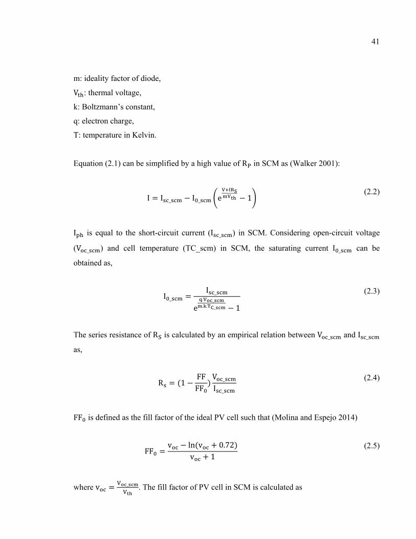
41
m: ideality factor of diode, V : thermal voltage,
k: Boltzmann’s constant,
q: electron charge,
T: temperature in Kelvin.
Equation (2.1) can be simplified by a high value of R in SCM as (Walker 2001):
I = I _ − I _ e − 1 (2.2)
I is equal to the short-circuit current (I _ ) in SCM. Considering open-circuit voltage
(V _ ) and cell temperature (TC_scm) in SCM, the saturating current I _ can be
obtained as,
I _ = I _e . _. . _ − 1 (2.3)
The series resistance of R is calculated by an empirical relation between V _ and I _
as,
R = (1 − FFFF ) V _I _ (2.4)
FF is defined as the fill factor of the ideal PV cell such that (Molina and Espejo 2014)
FF = v − ln(v + 0.72)v + 1 (2.5)
where v = _ . The fill factor of PV cell in SCM is calculated as
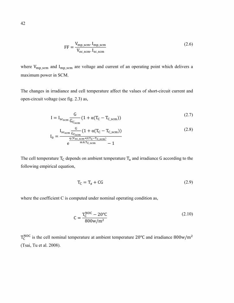
42
FF = V _ . I _V _ . I _ (2.6)
where V _ and I _ are voltage and current of an operating point which delivers a
maximum power in SCM.
The changes in irradiance and cell temperature affect the values of short-circuit current and
open-circuit voltage (see fig. 2.3) as,
I = I GG (1 + α(T − T _ )) (2.7)
I = I (1 + α(T − T _ ))e .( _ β( _ ). . _ − 1
(2.8)
The cell temperature T depends on ambient temperature T and irradiance G according to the
following empirical equation,
T = T + CG (2.9)
where the coefficient C is computed under nominal operating condition as,
C = T − 20800w/m (2.10)
T is the cell nominal temperature at ambient temperature 20 and irradiance 800w/m
(Tsai, Tu et al. 2008).

43
2.2.2. Solar module
The manufacturers provide PV cells into modules including Npm branches in parallel with
Nsm PV cells in series as illustrated in fig. 2.4 in order to achieve the desired output current
and voltage. The PV module current IM is implicitly described in (Chenni, Makhlouf et al.
2007):
= [1 − exp( − + . )] (2.11)
where: = . , module short-circuit current, = . , module open-circuit voltage, = . , module equivalent series resistance, = . , thermal voltage of module,
, PV module voltage.
MI
MV
smN
pmN
Figure 2.4 PV cells configuration in a module

44
Under standard (irradiance 1000W/m2, ambient temperature 25) or normal (irradiance
800W/m2, ambient temperature 20, wind speed 1m/s) conditions, the PV module
characteristics are given by manufacturers as illustrated in fig. 2.3.
2.2.3. Solar array
PV modules are connected in an array with Npa× Nsa elements as depicted in Figure 2.5.
Assuming that the modules are the same and the distribution of the irradiance on all modules
is uniform, the PV array terminal voltage and current are denoted as (Luque and
Hegedus 2011):
= N . = N .
(2.12)
This PV model as the part of microgrid model is developed and implemented in
Matlab/Simulink for simulation purposes.
AI
AV
saN
paN
Figure 2.5 PV module configuration in an array

45
2.3 DC-DC boost converter steady-state analysis:
The DC-DC boost converter circuit consists of a semiconductor power switch, diode and
inductor to transfer the energy from input to output. Control circuitry is added to the boost
converter to handle the energy transfer and to maintain the output in normal operating range.
The inductor stores the energy as a function of current (1Li ):
21 12
1LiLE =
(2.13)
pvUdcU
1L
pvC DCC1s
pviDi
1Li
Figure 2.6 DC-DC boost converter
The slew rate of current through the power switch is limited by the inductor. As a result the
stress on power switch due to the high peak current is limited by inductor. Switching
converters reveal higher efficiency than the linear power supplies which use the resistive
voltage drop to regulate the voltage (the power losses in the form of heat). The switching
regulator has a voltage drop and corresponding current which is 90° phase shift. The energy
as a result can be stored in charging period and recovered in discharge period respectively.
Figure 2.6 shows a simple configuration of a boost (step-up) converter. When the switch
closes, the inductor is in charge mode. The input voltage pvU is across the inductor so that its
current (1Li ) rises linearly at a rate as:

46
1
1
L
U
dt
di pvL = (2.14)
It is seen that the diode prevents the output capacitor voltage ( dcU ) from discharging. If the
switch opens, the inductor current flows into the rectification diode in order to charge the
output capacitor. This results in raising the output voltage at an inductor current rate as:
1
11
L
V
dt
di LL −= (2.15)
In steady state the average inductor voltage (<1LV >=0) is zero (equilibrium point) over the
entire switching cycle (Ts), i.e.,
0)(1
111
0
=+>=< sT
ON
ON
t
L
t
Ls
L dtVdtVT
V (2.16)
This volt-second rule implies that:
ONpvOFFL tUtV =1
(2.17)
Where tON and tOFF are the charge and discharge times of inductor respectively. Consider that
pvLdc UVU +=1
(2.18)
we can simplify the equation as:
pvOFF
ONdc U
t
tU )1( +=
(2.19)

47
Defining duty cycle D as:
OFFON
ON
tt
tD
+=
(2.20)
then the output voltage of boost converter in steady state is formulated as:
pvdc UD
U ]1
1[
−=
(2.21)
2.4 Photovoltaic Converter Dynamics
This section presents a detailed model which considers the converter transient response. A
DC-DC boost converter which connects the PV array to the DC bus is considered in Figure
2.6. The voltage of the capacitor at the terminal of the PV has the following dynamics,
= − 1 + 1
(2.22)
where and are the PV voltage and current, and is the inductor ( ) current. The
PV voltage, the inductor current and the DC bus voltage, are interrelated by the
following formula:
= 1 − 1 + (2.23)
where is a discontinuous signal which defines the converter switch position. The inductor
and capacitors and are considered to be known constants. Equations (2.22) and
(2.23) are essential in the design of a controller that regulates the DC-DC converter's input
voltage to a reference value that corresponds to the maximum power point of the PV system.

48
2.5 Voltage Source Inverter (VSI) and Space Vector Modulation (SVM):
A two-level Voltage Source Inverter (VSI) for three-phase system is considered in this thesis
as illustrated in Figure 2.7. Six power switches, SW1~SW6 with free-wheeling diodes in
parallel are contrived in the inverter. Each switching group consists of two or more power
switch devices (i.e. Insulated-Gate Bipolar Transistors (IGBTs) or MOSFETs) connected in
series depending on the DC input operating voltage level of the inverter. The selection of the
power switching devices depends on the switching frequency range, application power level
and acceptable power losses of the inverter. The desired output voltage of the inverter is
achieved by changing the frequency and amplitude of the reference signal. The comparison
between the references and the carrier waveforms results in Pulse Width Modulation (PWM).
This low level PWM signals from microcontrollers are translated to appropriate high voltage
level through DC-AC inverters. Among PWM techniques sinusoidal PWM (SPWM) and
Space Vector PWM (SVPWM) are known as popular modulation synthesis in inverter
applications.
Figure 2.7 Three-phase two-level voltage-source inverter
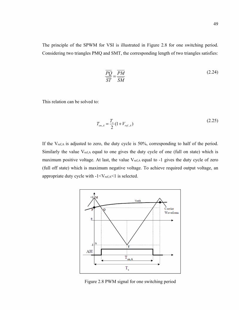
49
The principle of the SPWM for VSI is illustrated in Figure 2.8 for one switching period.
Considering two triangles PMQ and SMT, the corresponding length of two triangles satisfies:
SM
PM
ST
PQ = (2.24)
This relation can be solved to:
)1(2 ,, Aref
sAon V
TT +=
(2.25)
If the Vref,A is adjusted to zero, the duty cycle is 50%, corresponding to half of the period.
Similarly the value Vref,A equal to one gives the duty cycle of one (full on state) which is
maximum positive voltage. At last, the value Vref,A equal to -1 gives the duty cycle of zero
(full off state) which is maximum negative voltage. To achieve required output voltage, an
appropriate duty cycle with -1<Vref,A<1 is selected.
Figure 2.8 PWM signal for one switching period

50
Space vector modulation as one of the preferred real time modulation techniques is widely
used for digital control of VSIs. The operation of the inverter switches can be defined by
switching states. If the upper switches in inverter (Figure 2.7) are on, the switching state is
denoted by "H". As seen in Figure 2.7, the terminal voltage (VA, VB or VC) at each inverter
leg is Vd. Switching state "L" denotes the lower switches conduct with terminal voltage equal
to zero. There are eight states as listed in Table 2.1. For instance, the switching state [HLL]
denotes that the switches S1,S2, and S6 conduct in inverter phases. Two states of [LLL] and
[HHH] are defined as zero states while the others are active states. These active and zero
states can be demonstrated by six active space vectors 1V to 6V forming a hexagon with six
sectors I to VI. with the zero vector 0V on the center of the hexagon.
Table 2.1 Space Vector Modulation
Space vector Switching
state
Switch position
("on")
Vector definition
Zero vector 0V [HHH] or
[LLL]
(S1,S3, S5) or (S4,S6,
S2)
00 =V
Active vector 1V [HLL] (S1,S6, S2) 0
1 3
2 jd eVV =
Active vector 2V [HHL] (S1,S3, S2)
32 3
2 πj
deVV =
Active vector 3V [LHL] (S4,S3, S2)
3
2
3 3
2 πj
deVV =
Active vector 4V [LHH] (S4,S3, S5) πj
deVV3
24 =
Active vector 5V [LLH] (S4,S6, S5)
3
4
5 3
2 πj
deVV =

51
Active vector 6V HLH (S1,S6, S5)
3
5
6 3
2 πj
deVV =
Reference
vector
refV N.A. N.A. θjrefref eVV =
Assuming that the inverter is in three-phase balanced operation, we have the load phase
voltages as,
0)()()( =++ tVtVtV CNBNAN (2.26)
Equation (2.26) denotes that one of the phase voltages is redundant such that the third voltage
can be readily calculated. Therefore it is possible to transform the three-phase voltages to
equivalent two-phase voltages using Clarke transformation as:
−
−−=
)(
)(
)(
.
2
3
2
30
2
1
2
11
3
2)(
)(
tv
tv
tv
tV
tV
CN
BN
AN
β
α
(2.27)
The space vector can be represented in the α-β plane as:
)()( tjVtVV βα += (2.28)
For φφφ sincos je j += and 0=φ ,3
2π and 3
4π substituting Equation (2.27) into (2.28), we
have
++= 3
4
3
2
)()()(3
2 ππj
CN
j
BNAN etVetVtVV (2.29)

52
The phase voltages are calculated for the switching state [HLL] considering the balanced
three-phase system as,
dAN VtV3
2)( = , dBN VtV
3
1)( −= and dCN VtV
3
1)( −=
(2.30)
The space vector 1V therefore can be found by substituting (2.30) into (2.29) as,
01 3
2 jd eVV =
(2.31)
similarly the other active vectors can be derived as,
33
2 )1( π−= rjdr eVV , r=1,2,...,6
(2.32)
the Space vector diagram for the two-phase inverter is illustrated in Figure 2.9,
Figure 2.9 Space vector diagram for the two-level inverter

53
The active and zero vectors are stationary vectors and do not move in space while the
reference vector as illustrated in Figure 2.9 rotates in space at an angularly velocity ( fπω 2= )
where f is the fundamental frequency of the inverter output voltage. The next step is to
determine the duty-cycle time (on-state time) using the reference vector.
Assuming for the sufficiently small sampling time sT , the reference vector refV is constant
during sT . As demonstrated in Figure 2.9 refV can be approximated by two adjacent active
vectors and zero vector. Suppose refV falls into the sector I. Therefore refV can be obtained
by 1V , 2V and 0V . According to the volt-second balance, we have
0021 TVTVTVTV basref ++=
0TTTT bas ++=
(2.33)
where the parameters aT , bT and 0T are defined as the dwell times for the corresponding
vectors ( 1V , 2V and 0V respectively). Solving the equation according to table 2.1 yields
)3
sin(3
θπ −=d
refsa V
VTT
)sin(3
θd
refsb V
VTT = for
30
πθ <≤
bas TTTT −−=0
(2.34)
Defining the modulation index m such that,

54
d
ref
V
Vm
3=
(2.35)
Equation (2.34) can be expressed as,
)3
sin( θπ −= mTT sa
)sin(θmTT sb = for 3
0πθ <≤
bas TTTT −−=0
(2.36)
As the maximum of refV corresponds to the radius of the largest circle in hexagon shown in
Figure 2.9, the maximum magnitude of refV is obtained,
330cos.
3
2max ddref
VVV == °
(2.37)
That is the case of the maximum modulation index, 1max =m . The modulation index for the
space vector modulation is,
10 ≤≤ m (2.38)
The maximum fundamental line-to-line rms voltage modulated by SVM technique is
therefore calculated by,
dref
SVM VV
V 707.02
3max
max == (2.39)
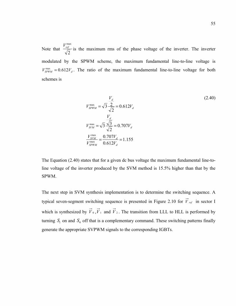
55
Note that 2
maxrefV
is the maximum rms of the phase voltage of the inverter. The inverter
modulated by the SPWM scheme, the maximum fundamental line-to-line voltage is
dSPWM VV 612.0max = . The ratio of the maximum fundamental line-to-line voltage for both
schemes is
155.1612.0
707.0
707.0233
612.02
23
max
max
max
max
==
==
==
d
d
SPWM
SVM
d
d
SVM
d
d
SPWM
V
V
V
V
V
V
V
V
V
V
(2.40)
The Equation (2.40) states that for a given dc bus voltage the maximum fundamental line-to-
line voltage of the inverter produced by the SVM method is 15.5% higher than that by the
SPWM.
The next step in SVM synthesis implementation is to determine the switching sequence. A
typical seven-segment switching sequence is presented in Figure 2.10 for refV in sector I
which is synthesized by 0V , 1V and 2V . The transition from LLL to HLL is performed by
turning 1S on and 4S off that is a complementary command. These switching patterns finally
generate the appropriate SVPWM signals to the corresponding IGBTs.

56
Figure 2.10 Seven-segment switching sequence
2.6 Inverter Voltage and Current Dynamics
A three-phase DC-AC inverter which connects the DC bus to the AC bus at the point of
common coupling (PCC) is illustrated in Figure 2.1. The voltages at the AC terminals of the
inverter, the currents through the filtering inductors ( ) and the voltages at the transformer
primary are related as follows,
= + ( ) (2.41)
where = ( , , ) and = ( , , ) are the three-phase voltage and current at
the inverter output, while ( ) = ( , , ) is the voltage at the transformer primary
side, as illustrated in Figure 2.1. Equation (2.41) is converted in the D-Q reference frame
using the Park transformation as follows, = + − ( ) (2.42)
= − + − ( ) (2.43)
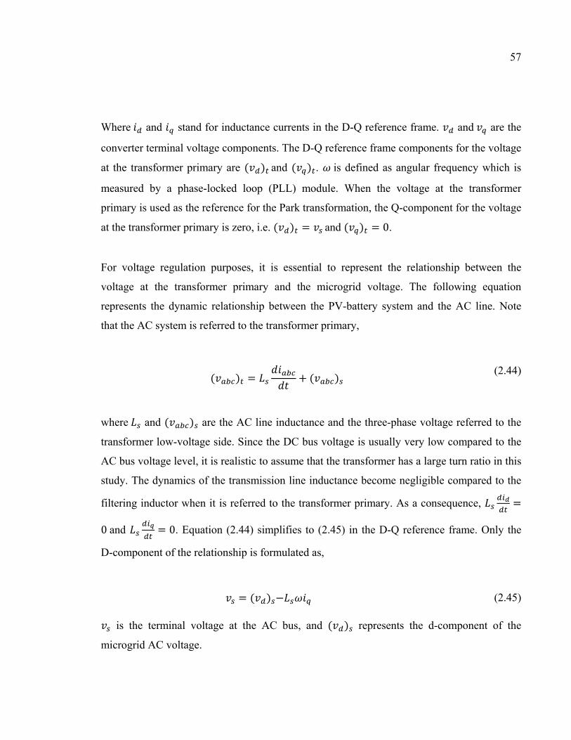
57
Where and stand for inductance currents in the D-Q reference frame. and are the
converter terminal voltage components. The D-Q reference frame components for the voltage
at the transformer primary are ( ) and ( ) . is defined as angular frequency which is
measured by a phase-locked loop (PLL) module. When the voltage at the transformer
primary is used as the reference for the Park transformation, the Q-component for the voltage
at the transformer primary is zero, i.e. ( ) = and ( ) = 0.
For voltage regulation purposes, it is essential to represent the relationship between the
voltage at the transformer primary and the microgrid voltage. The following equation
represents the dynamic relationship between the PV-battery system and the AC line. Note
that the AC system is referred to the transformer primary,
( ) = + ( ) (2.44)
where and ( ) are the AC line inductance and the three-phase voltage referred to the
transformer low-voltage side. Since the DC bus voltage is usually very low compared to the
AC bus voltage level, it is realistic to assume that the transformer has a large turn ratio in this
study. The dynamics of the transmission line inductance become negligible compared to the
filtering inductor when it is referred to the transformer primary. As a consequence, =0and = 0. Equation (2.44) simplifies to (2.45) in the D-Q reference frame. Only the
D-component of the relationship is formulated as,
= ( ) − (2.45)
is the terminal voltage at the AC bus, and ( ) represents the d-component of the
microgrid AC voltage.

58
2.7 Bidirectional Converter Voltage and Current Dynamics
The bidirectional DC-DC converter connected to the battery and the DC bus, as illustrated in
Figure 2.1 plays an important role in energy management in the microgrid. The DC bus
voltage ( ) dynamics are obtained through applying the Kirchhoff Current Law (KCL) at
the DC bus node,
= − − (2.46)
where , and are the diode current in the photovoltaic converter, the inverter input
DC current and the current through the inductor , respectively. Note that is the DC bus
capacitance. This gives in steady state:
= − (2.47)
Applying KVL to the battery converter circuit in Figure 2.1 gives the dynamics of the current
through inductor ,
= − (2.48)
where and are the battery terminal voltage and the converter switching position. The
two switches ( , ) have complementary positions in a manner when one is closed, the
other is open. In order to control the power flow among the PV, the battery, the synchronous
generator and the AC loads, it is essential to find the dynamics of the power exchanged in the
microgrid. These equations will relate the energy stored in the DC bus, the power generated
by the PV system, the power supplied by the battery and the power conveyed to the AC bus.
It can be shown that the energy stored in the DC bus ( ) satisfies the following equation,

59
= − − (2.49)
where = . , and are the power delivered by the PV to the DC bus,
the power delivered from the DC bus to the battery and the power sent to the AC side,
respectively. When the converter losses are ignored, the power at the battery output has the
following expression in terms of the inductor current and the DC bus voltage,
= (2.50)
Differentiating (2.50), multiplying both sides of the equality by and substituting
(2.48) and (2.49) yield,
= ( − − ) + 2 ( − ) (2.51)
Similarly when the DC-AC converter losses are neglected, the power exchanged between the
DC bus and the AC bus is equal to the power expression at the transformer primary. This
power has the following expression,
= 32 ( ( ) + ( ) ) (2.52)
where ( ) = and ( ) = 0 represent the terminal voltage at the primary side of the
transformer.

60
2.8 Synchronous machine model
This section aims to present the general structure of a conventional compensator of a
synchronous generator (SG) including excitation system and speed controller.
2.8.1 AVR, PSS and speed governor modules
One of the traditional excitation controls is the Automatic Voltage Regulator (AVR) that
compensates the terminal voltage. The AVR normally augments the field voltage to restore
the terminal voltage to its pre-fault level. Under large disturbances, due to a three-phase fault,
the terminal voltage of SG could be very low. After the faults are cleared the generator
reconnects to power system; however, this recovery causes post-fault oscillations due to the
energy stored in the generator rotor. Therefore another basic function of the excitation system
is to damp the oscillations. With addition of power system stabilizer (PSS) to the AVR, the
excitation system could eliminate any negative effect of damping post-fault oscillations (due
to the fast recovery of terminal voltage using the AVR).
The commonly used control signal of the PSS is the speed deviation as an additional
feedback signal for introducing a damping torque control component. Generally the PSS
includes the phase compensation module, which provides the phase-lead characteristic to
compensate for the phase lag between the exciter input and the generator electrical torque,
the high-pass wash-out filter, and the gain which determines the amount of damping
introduced by PSS. The PSS can generate a component of electrical torque which is in phase
with the rotor speed deviation. Thus, the oscillations corresponding to the rotor speed can be
detected and damped by the PSS. Figure 2.11 shows the excitation control system which is
combination of the PSS and the AVR.

61
Figure 2.11 PSS and AVR configuration in SG system
The basic function of the speed governor is to adjust prime mover output power for changes
in system speed. If the frequency decreases, due to load increment or loss of generation, the
speed of each connected generator will also decrease. The deviation in speed with respect to
its nominal value will be used to modify the position of the fuel valve. The objective is to
allow each generator to share the load power in interconnected power system. The droop
control and speed regulation are commonly used methods in synchronous generator governor
(see Figure 2.12). The term droop is the amount of the speed change necessary to cause the
prime mover control to move from fully closed to fully open position. In small isolated SGs,
the zero droop is considered such that the governor keeps the valve open until the speed is
restored to its nominal value. Therefore, speed droop is used to control the magnitude of
governor response for a given frequency change so all generators will share response after a
disturbance. On the other hand the definition of the speed regulation refers to the amount of
speed variation that is necessary to cause the output of the synchronous generator to change
from zero output to full output.
In contrast with droop, this term focuses on the output of the generator, rather than the
position of its valves.
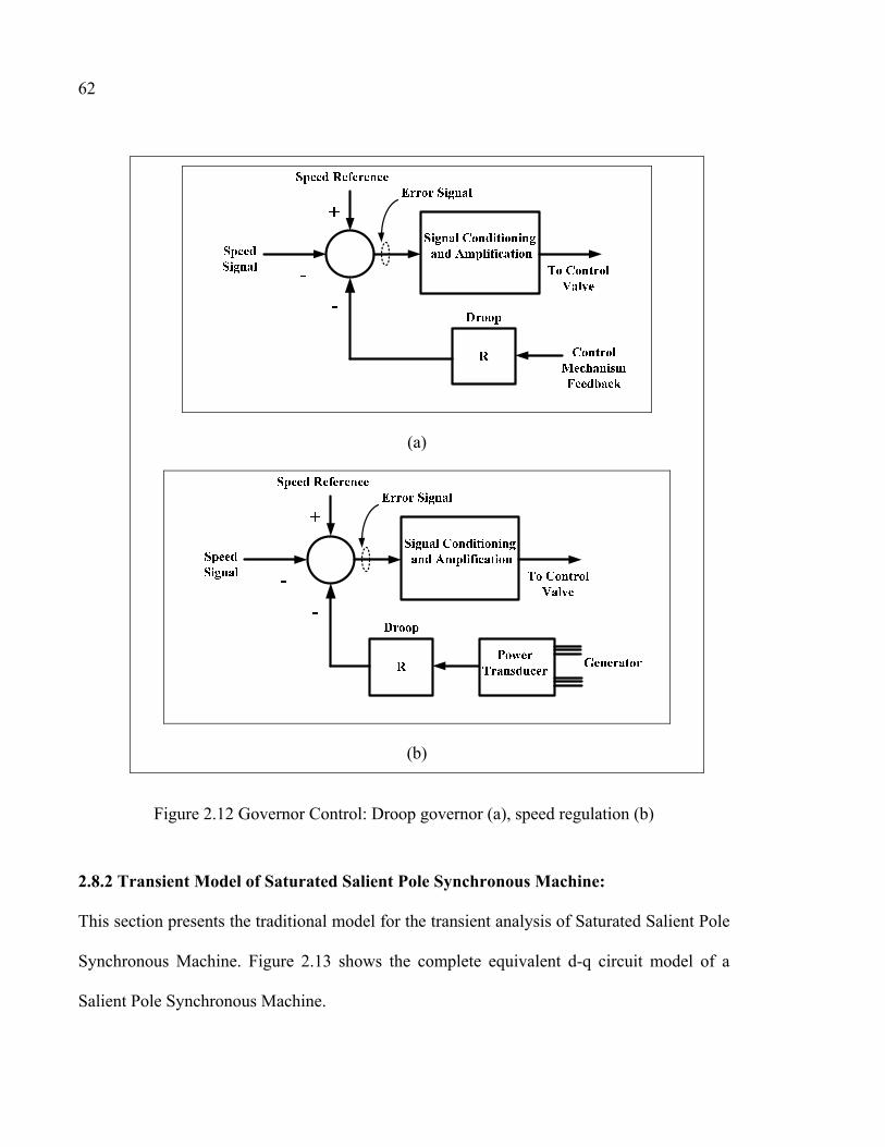
62
(a)
(b)
Figure 2.12 Governor Control: Droop governor (a), speed regulation (b)
2.8.2 Transient Model of Saturated Salient Pole Synchronous Machine:
This section presents the traditional model for the transient analysis of Saturated Salient Pole
Synchronous Machine. Figure 2.13 shows the complete equivalent d-q circuit model of a
Salient Pole Synchronous Machine.

63
qsv kqv
sr dsrλω saL
qscL
sbL
mqL
qrbL
qrcL
kqL1kqr
qsikqi
qssi+
−
(a)
dsv kdv
sr saL
dscL
sbL
mdL
drbL
drcL
kdL1kdr
dsi kdidssi
frr
fdL1
qsrλω
+
+
−
−frv
fdi
(b)
Figure 2.13 Salient Pole Synchronous Machine Model: Equivalent q-axis (a), Equivalent d-axis (b)
The d-q voltage equations in the rotor reference frame remain as follows:
fdb
fdfdfd
kdb
kdkdkd
kqb
kqkqkq
qsb
rds
bdssds
dsb
rqs
bqssqs
pirv
pirv
pirv
pirv
pirv
ψω
ψω
ψω
ψωωψ
ω
ψωωψ
ω
+=
+=
+=
−+=
++=
(2.53)

64
where operator p is the time derivative dtd . The flux linkages incorporating the effect of
saturation are given as follows:
( )( ) ( )
( )( ) ( )
( )( ) ( )
( )( ) ( )
( )satiX
satiXsat
satiX
satiXsat
satiX
satiXsat
satiX
satiXsat
satiX
drckdfdfd
mddrrdrbdrc
drckdkdkd
mqqrrqrbqrc
qrckqkqkq
mddsssbdsc
dscdssads
mqqsssbqsc
qscqssaqs
ψψψψ
ψψψψ
ψψψψ
ψψψψ
ψψ
+=+=
+=
+=
+=+=
+=
+=
+=
1
1
1
(2.54)
The flux linkages qsλ and dsλ have been multiplied by a base frequency bω to yield the d-q
stator flux linkages qsψ and dsψ . The variables qscψ , dscψ and qrcψ are the d, q stator core
and rotor core flux linkages respectively. The variables kdψ and fdψ are the d-axis flux
linkages of the damper and field windings respectively, and kqψ represents the q-axis damper
flux linkage. The machine currents are derived as follows:
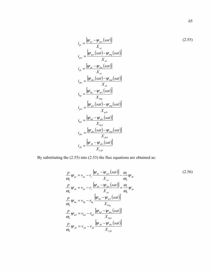
65
( )[ ]
( ) ( )[ ]
( )[ ]
( ) ( )[ ]
( )[ ]
( ) ( )[ ]
( )[ ]
( ) ( )[ ]
( )[ ]fd
drcfdfd
drb
mddrcdrr
kd
drckdkd
qrb
mqqrcqrr
kq
qrckqkq
sb
mddscdss
sa
dscdsds
sb
mqqscqss
sa
qscqsqs
X
sati
X
satsati
X
sati
X
satsati
X
sati
X
satsati
X
sati
X
satsati
X
sati
1
1
1
ψψ
ψψ
ψψ
ψψ
ψψ
ψψ
ψψ
ψψ
ψψ
−=
−=
−=
−=
−=
−=
−=
−=
−=
(2.55)
By substituting the (2.55) into (2.53) the flux equations are obtained as:
( )[ ]
( )[ ]
( )[ ]
( )[ ]
( )[ ]fd
drcfdfdfdfd
b
kd
drckdkdkdkd
b
kq
qrckqkqkqkq
b
qsb
r
sa
dscdssdsds
b
dsb
r
sa
qscqssqsqs
b
X
satrv
p
X
satrv
p
X
satrv
p
X
satrv
p
X
satrv
p
1
1
1
ψψψ
ω
ψψψω
ψψψ
ω
ψωωψψψ
ω
ψωωψψ
ψω
−−=
−−=
−−=
+−−=
−−
−=
(2.56)

66
The unsaturated magnetizing flux in the q and the d axes are as follows:
( ) ( )( ) ( )drrdssmdmd
qrrqssmqmq
iiXunsat
iiXunsat
+=
+=
ψψ
(2.57)
The saturated magnetizing flux in the q and the d axes are given:
( ) ( )( ) ( )
( ) ( )( ) ( )unsatK
unsatK
unsatsat
unsatsat
mdmdmd
mqmqmq
mdmdmd
mqmqmq
ψψψψ
ψψψψψψ
−=Δ
−=ΔΔ−=
Δ−=
1
1
(2.58)
where the mqK and mdK are the saturation factors for magnetizing flux in the q and the d
axes. The total unsaturated magnetizing flux is given as:
( ) ( ) ( )unsatunsatunsat mdmqm22 ψψψ += (2.59)
By substituting the (2.55) into (2.57) the unsaturated flux equations are obtained as:
( )
( ) mddrbsb
mdddrb
drc
sb
dscmddmd
mqqrbsb
mqqqrb
qrc
sb
qscmqqmq
XXX
XXXunsat
XXX
XXXunsat
ψψψψ
ψψψ
ψ
Δ
++
+=
Δ
++
+=
11
11
(2.60)
where

67
++
=
++
=
drbsbmq
mdd
qrbsbmq
mqq
XXX
X
XXX
X
111
1
111
1
(2.61)
The unsaturated core flux equations are given:
( ) ( )( ) ( )( ) ( )( ) ( )drrfdkddrcdrc
qrrkqqrcqrc
dssdsscdsc
qssqsscqsc
iiiXunsat
iiXunsat
iiXunsat
iiXunsat
−+=
−=−=
−=
ψψψψ
(2.62)
By substituting the current equations (2.55) into (2.62) the above unsaturated flux equations
are obtained as:
( )
( )
( ) ( )
( ) ( )qrc
qrbfqkqqrcc
qrb
mq
fq
fq
kq
kqqrccqrc
drcdrbfdkd
drccdrb
md
fd
fd
kd
kddrccdrc
qscsbsasb
mq
sa
qssccqsc
dscsbsasb
md
sa
dssccdsc
XXXX
X
sat
XXXunsat
XXXX
X
sat
XXXunsat
XXXXXunsat
XXXXXunsat
ψψψψ
ψ
ψψψψψ
ψψψ
ψ
ψψψψ
Δ
+++
++=
Δ
+++
++=
Δ
++
+=
Δ
++
+=
111
111
11
11
1111
1111
(2.63)
where

68
++
=
+++
=
++
=
qrbkqqrc
qrcc
drbfdkddrc
drcc
sbsasc
scc
XXX
X
XXXX
X
XXX
X
111
1
1111
1
111
1
1
11
(2.64)
The changes in the flux linkages in the core due to saturation are given as:
( ) ( )( ) ( )( ) ( )( ) ( )unsatK
unsatK
unsatK
unsatK
drcdrdrc
qrcqrqrc
dscsdsc
qscsqsc
ψψψψψψψψ
−=Δ
−=Δ−=Δ
−=Δ
1
1
1
1
(2.65)
The saturated core flux linkages are written as:
( ) ( )( ) ( )( ) ( )( ) ( ) drcdrcdrc
qrcqrcqrc
dscdscdsc
qscqscqsc
unsatsat
unsatsat
unsatsat
unsatsat
ψψψψψψψψψψψψ
Δ−=
Δ−=Δ−=
Δ−=
(2.66)
where the parameter sK is the saturation factor for the stator core and is a function of the
total unsaturated stator core flux linkage as:
( ) ( ) ( )unsatunsatunsat dscqscsc22 ψψψ += (2.67)
The rotor saturation factors drK and qrK are defined similarly.

69
The electromagnetic torque with poles number P is given as:
[ ]dsqsqsdsb
e iiP
T ψψω
−=22
3
(2.68)
2.8.3 Swing equation:
The swing equation neglects all electrical dynamics, considered much faster than mechanical
dynamics. The equation of motion of the synchronous machine rotor that is driven by a prime
mover is given by:
aem TTTdt
dJ =−=
2
2θ
(2.69)
where:
J is the total moment of inertia of the rotor mass in kgm2;
Tm is the mechanical torque supplied by the prime mover in N-m;
Te is the electrical torque output of the alternator in N-m;
θ is the angular position of the rotor in rad.
If mechanical and electrical torques are exactly equal, there can be no angular acceleration,
and this is the case when the machine is in synchronism, i.e.,
em TT = (2.70)
During this period the rotor will move at synchronous speed ωs in rad/s. When there is a
difference between mechanical and electromagnetic torques, the machine accelerates. The
amount of acceleration is proportional to the difference between Tm and Te. This difference is
called the accelerating torque Ta,

70
ema TTT −= (2.71)
We define ωr as the rated mechanical angular velocity of the shaft, in rad/sec such that
2/Pe
r
ωω = (2.72)
where P is the number of poles. We also define a synchronously rotating reference frame as:
αωθ += trref (2.73)
where α is the initial angle. Derivation of Equation (2.73) gives,
rrefdt
d ωθ = (2.74)
This implies that the reference speed is constant. Let us define the rotor mechanical torque
angle, mδ as,
refm θθδ −= (2.75)
Where θ and refθ designate rotor and reference positions respectively. The above relation is
illustrated in Figure 2.14.

71
Figure 2.14 Rotor angular position with respect to the reference position in phase-a of synchronous machine
The position mδ is the angle of the internal voltage of a synchronous machine (see Figure
2.15) and it corresponds to the amount of power that can be transferred. This angle is called
the load angle.
mE δ∠ °∠ 0V
X
Figure 2.15 Per-phase equivalent circuit of the three-phase synchronous machine
We can rewrite the Equation (2.75) as
mrt δαωθ ++= (2.76)
Considering the transient condition, by taking the first derivative of (2.76), we have:

72
mr dt
d
dt
d δωθ += (2.77)
The second derivative results in
mdt
d
dt
d δθ2
2
2
2
= (2.78)
Therefore the Equation (2.78) can be written as
aemm TTT
dt
dJ =−=
2
2δ
(2.79)
Equation (2.79) describes the behavior of the rotor dynamics and hence is known as the
swing equation. For the general case of P-pole machine we have the Equation (2.79) in
electrical radian as,
aeme TTT
dt
d
PJ =−=
2
22 δ
(2.80)
Since 2
2
dt
d
dt
d ee δω = , finally the swing equation for the synchronous machine can be written
as:
aeme TTT
dt
d
PJ =−=ω2
(2.81)
2.9 Frequency and voltage models
The frequency model is essential for the proposed model-based design strategy. Since the
frequency is proportional to the synchronous generator rotor speed, the frequency dynamics
are obtained from the well-known swing equation (i.e. 4-pole machine):

73
12 = − − (2.82)
where , and are the synchronous generator mechanical speed, the inertia and friction
coefficient, respectively. is the synchronous generator output power and is the
mechanical power. The synchronous generator power, the load power and the power
generated by the PV-battery system are related by the algebraic relationship:
= + (2.83)
The mechanical power is provided by a prime mover. It is assumed that the synchronous
generator is equipped with its own automatic voltage regulator (AVR) and speed governor
which has droop characteristics. Therefore, the following relationship between the
mechanical power and the mechanical speed can be assumed,
= − − + = − ∆ + (2.84)
is the reference power for the speed governor of the synchronous generator. Let the
frequency
= = 2
(2.85)
where is the number of pole pairs.
The frequency dynamical model has the following expression:
= 2 − ∆ + − − 32 − (2.86)

74
To considerably reduce the steady state error of the voltage at the transformer primary, an
integrator is added to the voltage control loop. This requires defining a new variable which is
the integral of the voltage deviation from its reference value.
Ω = − (2.87)
The dynamics of this new variable are given by the following equation which is added to the
model presented in this section. dΩ = ( ) − − (2.88)
2.10 Nonlinear model of the entire system
Equations (2.22), (2.23), (2.42), (2.43), (2.49), (2.51), (2.86), and (2.88) represent the
dynamic model of the hybrid PV-Battery generator. This model has eight states and four
inputs/outputs. It can be rewritten in the following closed form,
x = ( ) + ( ) y = ℎ( ) (2.89)
where = [ , , , Ω, , , , ] is the vector of state variables, =[ , , , ] is the vector of control inputs, and = ℎ( ) = [ , Ω, , ] is the vector
of outputs. The nonlinear vector function ( ) and the matrix ( ) are given as:

75
( ) =
− 1 + 11 − 1−( ) − −− − 32( − − 32 ) + 2+ −2 − ∆ + − − 32 −
( ) =
0000000
00 100000
00000−200
000000 10
(2.90)
This model is nonlinear, multivariable and highly coupled with the independent variables , , , Ω, , , and .The model is used in next chapters for designing advanced
nonlinear control.

76
2.11 Conclusion
This chapter firstly described the commonly used models of a PV system (i.e. PV
cell/module/array), power electronic converters (i.e. modulation techniques, steady-state and
dynamic analysis), synchronous generator (i.e. voltage vs. speed control, transient and
saturation model and swing equation) and frequency model. It was followed by proposing a
novel mathematical model (8th order) of a PV-battery generator in a microgrid paralleled with
synchronous generator. This suggested model, in addition to the nonlinear model of PV
array, is nonlinear, multivariable and highly coupled. This model is used for designing an
innovative and advanced control technique.
CHAPTER 3
CLASSICAL CONTROL OF MICROGRID
3.1 Introduction
This chapter proposes a classical control approach based on backstepping control technique
composed of a group of several cascaded control loops. The control strategy will not use the
complete nonlinear model that was presented in chapter 2. To tackle the microgrid (MG)
problems discussed in the introduction of this thesis, the control scheme is structured into
three controller modules: (i) three-phase dc-ac inverter (i.e. decoupled frequency and voltage
controller), (ii) photovoltaic dc-dc converter (i.e. maximum power point tracking controller)
and (iii) battery dc-dc converter (i.e. DC bus voltage controller). The proposed classical
approach offers advantages over existing ones as the PV generator emulates the reaction of a
conventional generator in frequency and voltage regulation. The motivation of the classical
control is to propose a method of MG control which doesn't use the exact nonlinear model
suggested in previous chapter. The frequency, as a global state variable is formulated by a
droop characteristics. The charging or discharging decision is made by a simple algorithm
based on the state of the power of the PV and the load. The simplicity and independence of
the controllers allow for an extension to more complex and large-scale microgrid which is a
significant advantage. The controller performance is evaluated in simulation using the
SimPowerSystems blockset in Simulink/Matlab.
3.2 Microgrid System and Control
The proposed microgrid in this chapter, as presented in Figure 3.1, includes a PV array, a
battery storage, a synchronous generator and a load. The primary objective is that the hybrid
PV-battery system participates in frequency and voltage regulation just as the synchronous
generator does despite the power changes from either the local sources (i.e. insolation
variation) or the load perturbation. This primary objective is associated with the control of
the dc-ac inverter: (i) cascaded frequency and power controller and (ii) cascaded terminal

78
voltage and current controller. It is then followed by designing cascaded control of battery to
regulate the dc bus voltage as well as the battery current. Finally the design of a classical
maximum power point tracker (i.e. Perturb & Observe (P&O) method) and cascaded
controller for the PV system is suggested.
Figure 3.1 General configuration of the suggested microgrid
3.2.1 Inverter control
This section presents the design of frequency and terminal voltage control modules. The
frequency control is based on droop technique along with the design of active power control
module. The reference of the power control module is modified by suggested droop control.
The terminal voltage control is based on backstepping control (Okou 2012) with inner
current control loop.
Frequency control design:
Conventionally, the imbalance in active power between generation and demand in a
microgrid (MG) causes the frequency deviation. Consider the power flow transferred by a
transmission line between two generators as depicted in Figure 3.2,
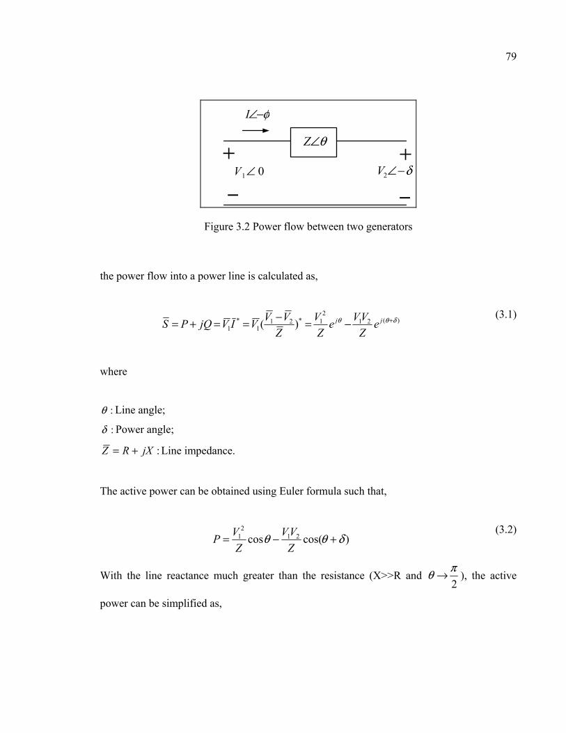
79
01∠V δ−∠2V+
− −
θ∠Z
φ−∠I
+
Figure 3.2 Power flow between two generators
the power flow into a power line is calculated as,
)(212
1*211
*1 )( δθθ +−=−==+= jj e
Z
VVe
Z
V
Z
VVVIVjQPS
(3.1)
where
:θ Line angle;
:δ Power angle;
:jXRZ += Line impedance.
The active power can be obtained using Euler formula such that,
)cos(cos 212
1 δθθ +−=Z
VV
Z
VP
(3.2)
With the line reactance much greater than the resistance (X>>R and 2
πθ → ), the active
power can be simplified as,

80
δsin21
X
VVP =
(3.3)
If the power angle δ is small, then δδ ≅sin . Rewriting the Equation (3.3) gives,
δX
VVP 21≅
(3.4)
Linearizing (3.4) around equivalent points ( 0δ ) using Taylor series, assuming 00 =δ gives,
δΔΓ≅Δ .pP
(3.5)
where coefficient pΓ is given by
X
VVp
02
01 .
=Γ
(3.6)
The active power can be therefore controlled through regulation of the power angle.
Frequency control leads to regulate the power angle and this in turn controls the real power
flow (Alvaro et al. 2011). Assuming linear relationship (Emadi, A. et al. 2004) between the
power angle and frequency ( fΔ=Δ .αδ ), Equation (3.5) can be rewritten as,
fP p ΔΓ≅Δ ..α (3.7)
This observation leads to droop characteristics such that,

81
fkP Δ−=Δ .1 (3.8)
where k1 is the droop gain of the MG characteristics discussed in Chapter 2. The first order
model of frequency deviation with decoupled active power deviation is obtained.
Considering the first-order measurement filters with small time constant T1, the variables ∆ which is the measured frequency is given as:
∆ = 11 + ∆
(3.9)
As illustrated in Figure 3.5, the deviations of active power of the PV-battery (i.e. ∆ ) is
added to the corresponding power produced by conventional generator (i.e. synchronous
generator,∆ ) in order to reduce the deviation in load power (∆ ). The power deviation ∆ is defined as,
∆ = − − ∗
(3.10)
Note that in above formulation, a high efficient converter design with negligible power losses
is assumed to be used. This implies that the apparent power deviation ∆ converges to zero
in steady state when the power balance meets in islanded microgrid.
The proposed control offers both the dynamic and steady state power participation of PV
generator to restore the frequency and voltage. In fact, a bigger compensation coefficient is
needed to damp the initially fast power variation. In case of load increase or decrease,
respectively a high positive or negative equivalent compensating signal is chosen to damp the
deviation to a prescheduled rating range. On the contrary, the slow continuous power
changes need smaller coefficient. On the other hand, very large values of a compensation
index in steady state results in instabilities in the microgrid, while small values cause big
frequency drop so that the inverter trips off. Therefore the selection of a dynamic index plays
an important role in microgrid performance. This section proposes a multi-rate curve so that

82
a dynamic coefficient is chosen to damp both fast and slow power variation. A dead zone
with zero droop is defined for the slight frequency variation, thus the microgrid is maintained
at its rated power.
According to the compensation characteristic shown in Figure 3.3, the proposed curve is
divided into three regions: (i) high load sharing (positive droop), (ii) rated load sharing (zero
droop) and (iii) low load sharing (negative droop). At the beginning of the load increment, a
fast power injection is supported by a big compensating gain (positive). It can therefore
compensate the frequency fluctuation caused by the inrush load power until the deviation is
maintained in an acceptable range. Then the PV generator supports the load by the small
compensating index with its nominal power participation. This strategy provides enough time
for conventional generators to participate into the load power sharing. On the contrary, in a
condition when the load is decreasing or the generation power of the microgrid is higher than
the load power demand, the negative compensating index updates the deviation references to
avoid the over frequency and to maintain power balance. The strategy provides an automatic
feature of load sharing for the PV generation unit. Note that the frequency and angle are
estimated by phase-locked loop (PLL) module.
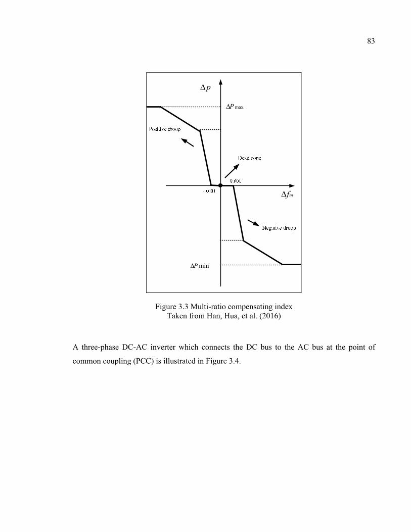
83
pΔ
maxPΔ
mfΔ
minPΔ
Figure 3.3 Multi-ratio compensating index Taken from Han, Hua, et al. (2016)
A three-phase DC-AC inverter which connects the DC bus to the AC bus at the point of
common coupling (PCC) is illustrated in Figure 3.4.

84
Lr
L
LAi
Lr
L L
Lr
LBiLCi
*ad *
bd*cd
pccav pcc
bv pcccv
Figure 3.4 Three-phase inverter
pΔ dv preff
s
1
f
td
L
v
2
)(3
tddf
tdtdq v
dt
di
L
vvi )(
2
3
2
)(3)(
2
3 2 +−ω
mf
refp
*pmfΔ
Figure 3.5 Control structure for inverter; frequency loop control with inner power loop control
85
Power controller design:
To maintain the ac power generated by PV-battery generator close to its reference value, the
output power dynamics are required. The dynamics for the active power have the following
expression,
dp = ( ) + ( ) dp = ( ) + − ( ) + ( )
(3.11)
These power dynamics are nonlinear. Therefore, the following power control law is
proposed.
= ( ) − − + ∗ − ( ) − ( ) − ( ) (3.12)
The parameter is positive gain. Substituting (3.12) into (3.11) gives the following closed
loop dynamics.
dp = − − + ∗ (3.13)
The system represented by (3.13) is stable for any positive gain. The variable is the
reference value for the active power. The reference variable ∗ is modified by the frequency
control module when the frequency deviation becomes large.

86
Terminal voltage controller design:
To maintain the terminal voltage close to its reference value, the following variable which
represents the integral of the voltage deviation is introduced.
Ω = − (3.14)
The dynamics for this new variable have the following expression when the power
expression is substituted.
dΩ = ( ) − − (3.15)
Equation (3.15) is used to find the value of the q-axis current so that the terminal voltage
converges to its reference value. To facilitate the design, the following error variable is
given,
∆ = − ∗ (3.16)
Substituting (3.16) into (3.15) gives the following dynamics,
dΩ = ( ) − ∗ − ∆ − (3.17)
The value that the inductor current must have so that the error dynamics converge to zero
has the following expression,
∗ = − − Ω −( ) + (3.18)

87
The parameter is positive gain. Substituting (3.18) into (3.17) gives the following closed
loop dynamics.
dΩ = − Ω − ∆ (3.19)
The objective is to find the input value so that converges to its reference value ∗ . The
error dynamics have the following expression,
∆ = − + 1 − ∗ (3.20)
This equation is used to find the expression for the control input so that the current error
dynamics converge to zero as,
= − ∆ + Ω + + ∗ (3.21)
The parameter is positive gain. Substituting (3.21) into (3.20) gives the following closed
loop dynamics.
∆ = − ∆ + Ω (3.22)
It is simple to prove that the closed loop system which includes the recursive voltage and
current controllers is stable. The closed loop dynamics have the following form:

88
dΩ = − Ω − ∆
∆ = − ∆ + Ω
(3.23)
The following positive definite Lyapunov function is used:
= Ω + ∆ (3.24)
The derivative of this Lyapunov function has the following expression
= −2 Ω − 2 ∆ (3.25)
The closed loop system (3.23) is therefore asymptotically stable since the (3.25) is negative
definite. As a consequence error signals converge asymptotically to zero. Figure 3.6
demonstrates the structure of the suggested cascaded terminal voltage control based on
backstepping control method (Okou 2012).
fsL
1 svrefsv svΔ *
qi
qiqiΔ qv
df iL ω
ωsL
sdv )(
s
1
VΩ
Figure 3.6 Control structure for inverter (vq); terminal voltage loop control with inner current loop control

89
3.2.2 Battery converter control
A backup system is considered for the proposed microgrid system to reserve power when the
load demand is lower than the generation and to support the microgrid when more generation
power is requested. On the other hand, to avoid the mismatching power between generation
and demand, it is important to use a battery in the microgrid design rather than load dumping
approaches. A DC-DC converter is used to connect the battery to the rest of the microgrid
system at DC bus connection (Figure 3.7).
batU dcU
2L
batC DCC
batiouti2Li
22s
av
ci
eqR21s
Figure 3.7 Bidirectional DC-DC converter
This section presents a control approach to charge and discharge the battery while
contributing into the frequency and voltage regulation introduced in previous section. Figure
3.8 demonstrates a cascaded battery controller consisting of an outer DC bus voltage
regulator and an inner current regulator. The goal to maintain the power balance at DC bus is
obtained by regulating the DC bus voltage. The dc-dc converter model as presented in
chapter 2 is:
= − −
= −
(3.26)

90
Udc controller design:
The Equation (3.26) is used to design this controller. The objective is to find the value the
inductor current must have so that the DC bus voltage converges to its reference
value ∗ . The following error variable is therefore defined to facilitate the design.
∆ = − ∗ ∆ = − ∗
(3.27)
which , ∗ and ∆ are inductor current, its reference and error dynamics. The error
dynamics ∆ have the following expression,
∆ = 1 − 1 − 1
(3.28)
The value that the inductor current must have so that the error dynamics converge to zero has
the following expression,
∗ = − − ∆ − ( 1 − 1 ) (3.29)
The parameter is positive gain. Substituting (3.29) into (3.28) and considering= ∆ + ∗ gives the following closed loop dynamics.
∆ = − ∆ − 1 ∆ (3.30)

91
The system represented by (3.30) is stable for any positive gain. The controller output will
become the input of the inductor current controller. Next section discusses how this
controller equation is obtained.
controller design:
Equation (3.26) is used for the design. The objective of the controller is to maintain the
inductor current to its reference ∗ which is obtained from the previous control module.
The following error variable is defined to facilitate the design.
∆ = − ∗ (3.31)
The error dynamics have the following expression,
∆ = 1 − 1 − ∗ (3.32)
The controller equation is deduced from Equation (3.32). It has the following form,
= [ . ∆ − 1 ∆ + 1 − ∗ ] (3.33)
The parameter is positive gain. Substituting (3.33) into (3.32) gives the following closed
loop dynamics. ∆ = − . ∆ + 1 ∆ (3.34)
It is simple to prove that the closed loop system which includes the recursive voltage and
current controllers is stable. The closed loop dynamics have the following form:

92
∆ = − . ∆ + 1 ∆
∆ = − ∆ − 1 ∆
(3.35)
The following positive definite Lyapunov function is used:
= ∆ + ∆ (3.36)
The derivative of this Lyapunov function has the following expression
= −2 ∆ − 2 ∆ (3.37)
The closed loop system (3.35) is therefore asymptotically stable since the (3.37) is negative
definite. As a consequence error signals converge asymptotically to zero. When the voltage
at DC bus is high, the controller reduces its discharging power by reducing the current
reference and vice versa. As this voltage controller provides the reference for the current
controller, the outer voltage controller should be slower than the inner current controller.
Note that in Figure 3.8 is defined as,
= = − (3.38)
A "seamless" charging-discharging mechanism of the proposed bidirectional dc-dc converter
is based on dc bus voltage regulation. If > the converter controller turns to

93
charging mode that is = 0and is equal to modulation of which is the controller
output. If < , the converter controller turns to discharging mode that is = 0and
is equal to modulation of which is the controller output. On the other hand this leads
to energy balance at the dc bus.
2
1
sLdcsC
1 dcv*dcv
dcvΔ *
2Li
2Li2LiΔ dcCiav
batteqR
1batteqi
Figure 3.8 Control structure for battery converter; Voltage loop control with inner current loop control
3.2.3 Photovoltaic converter control
Because of the nonlinear characteristics of the PV array system and the intermittent condition
of the weather, the PV optimal operating point is unknown and it should be estimated using
maximum power point tracker (MPPT). This process is conducted simultaneously with a
controller (a cascaded regulator) to change the duty cycle which commands the DC-DC
converter connected to the PV array. Figure 3.9 shows the PV converter diagram.
pvUdcU
1L
pvC DCC1s
pviDi
1Libv
Figure 3.9 Photovoltaic dc-dc converter

94
As presented in chapter 2, the model of dc-dc converter is given,
= − 1 + 1
= 1 − 1 +
(3.39)
1
1
sLpvsC
1
pveqR
1
pvv*pvv
pvvΔ
1Lipv
eqi
pvCibvpvi
*
1Li1LiΔ
Figure 3.10 PV converter control; Maximum power point tracker (MPPT), voltage loop control with inner current loop control
Upv controller design:
The Equation (3.39) is used to design this controller. The objective is to find the value the
inductor current must have so that the PV voltage converges to its reference value ∗ given by MPPT module. The following error variable is therefore defined to facilitate the
design.
∆ = − ∗ ∆ = − ∗
(3.40)

95
which , ∗ and ∆ are inductor current, its reference and error dynamics. The error
dynamics ∆ have the following expression,
∆ = − 1 + 1 − ∗ (3.41)
The value that the inductor current must have so that the error dynamics converge to zero has
the following expression,
∗ = − [− . ∆ − 1 + ∗ ] (3.42)
The parameter is positive gain. Substituting (3.42) into (3.41) and considering= ∆ + ∗ give the following closed loop dynamics.
∆ = − . ∆ − 1 ∆ (3.43)
The controller output will become the input of the inductor current controller. Next sections
discuss how this controller equation is obtained.
controller design:
Equation (3.39) is used for the design. The objective of the controller is to maintain the
inductor current to its reference ∗ which is obtained trom the previous control module.
The following error variable is defined to facilitate the design.

96
∆ = − ∗ (3.44)
The error dynamics have the following expression,
∆ = 1 − 1 + − ∗ (3.45)
The controller equation is deduced from Equation (3.45). It has the following form,
= [− . ∆ + 1 ∆ − ( 1 − 1 − ∗ )] (3.46)
The parameter is positive gain. Substituting (3.46) into (3.45) gives the following closed
loop dynamics.
∆ = − . ∆ + 1 ∆ (3.47)
It is simple to prove that the closed loop system which includes the recursive voltage and
current controllers is stable. The closed loop dynamics have the following form:
∆ = − . ∆ + 1 ∆
∆ = − . ∆ − 1 ∆
(3.48)
The following positive definite Lyapunov function is used:

97
= ∆ + ∆ (3.49)
The derivative of this Lyapunov function has the following expression
= −2 ∆ − 2 ∆ (3.50)
The closed loop system (3.48) is therefore asymptotically stable since the (3.50) is negative
definite. As a consequence error signals converge asymptotically to zero. Note that in Figure
3.10 is defined as,
= (3.51)
∗ MPPTdesign:A conventional MPPT (Hua, Chihchiang et al. 1998) is chosen in this chapter to guarantee
that the PV array operates at the optimal voltage while delivers its peak power. The perturb
and observe (P&O) method is probably the most often used MPPT algorithm today, due to its
simplicity and generic nature. It is based on the fact that the derivative of power in function
of voltage is zero at MPP. At an operating point on the P–V curve, if the operating voltage of
the PV array is perturbed in a given direction and 0>Δ pvP , it is known that the perturbation
moved the array’s operating point toward the MPP. The P&O algorithm would then continue
to perturb the PV array voltage in the same direction. If 0<Δ pvP , then the change in
operating point moved the PV array away from the MPP, and the P&O algorithm reverses the
direction of the perturbation. Figure 3.11 demonstrates the P&O operation. Note that k and k-
1 are the actual and previous sampling instances respectively. Since the P&O technique is

98
based on sequential perturbation, unwanted disturbance or noise on sensors could confuse
this MPPT. To avoid this problem, a very mall threshold η is considered in this MPPT
design. As known, the operating point oscillates around the MPP with amplitude of C (see
Figure 3.11). The output of this Upv-reference generator becomes the input of the Upv-
controller whose design was presented in the previous sections.
Figure 3.11 Flowchart of the MPPT based on P&O method
Start
Measure )1( −kvpv
)1( −kipv
)1(* −= kvv pvpv
)1().1()1( −−=− kikvkp pvpvpv
Measure )(kvpv
)(kipv
)(* kvv pvpv =
)().()( kikvkp pvpvpv =
)1()()( −−=Δ kpkpkp pvpvpv
η>Δ )(kppv
Cvv pvpv += **Cvv pvpv −= **
YESNO

99
3.3 Results and Discussion
To validate the proposed control system, a microgrid is simulated in MATLAB/SIMULINK
using its detailed model. Considering the diagram illustrated in Figure 3.1, the microgrid
includes a synchronous generator, photovoltaic array generator, battery unit and load. The
system parameters are presented in Table 3.1. Several scenarios with changes of loads and
insolation are considered in this study in order to examine the performance of the control
system with frequency and voltage control of microgrid and the load sharing capability
between DC and AC microgrid. The synchronous generator is assumed to have its own speed
governor as well as automatic voltage regulator (AVR).
Both active and reactive power of the load increase 20% at time 100s to evaluate the
performance of the frequency and voltage controller.
The amplitude of AC bus voltage at the point of common coupling, PCC is controlled as
shown in Figures 3.12 during adding of the load power (time 100s). Figure 3.12 shows that
the terminal voltage starts to deviate during a transient time 0.8 s after load disturbance at
time 100 s but it maintains at its nominal set point by contribution of reactive power (see
Figure 3.14) from both PV and SG.
Figure 3.12 Terminal voltage performances under load increment
99.8 100 100.2 100.4 100.6 100.80.97
0.975
0.98
0.985
0.99
0.995
1
1.005
Time(s)
AC
bu
s vo
ltag
e(p
u)

100
(a)
(b)
Figure 3.13 Active powers variation; hybrid PV & battery (a), synchronous generator (b) under load increment
90 100 110 120 130 140 150 160 170 1800.08
0.09
0.1
0.11
0.12
0.13
0.14
0.15
0.16
Time(s)
PV
act
ive
pow
er(p
u)
90 100 110 120 130 140 150 160 170 180 1900.08
0.1
0.12
0.14
0.16
0.18
0.2
0.22
0.24
Time(s)
SG
act
ive
pow
er(p
u)
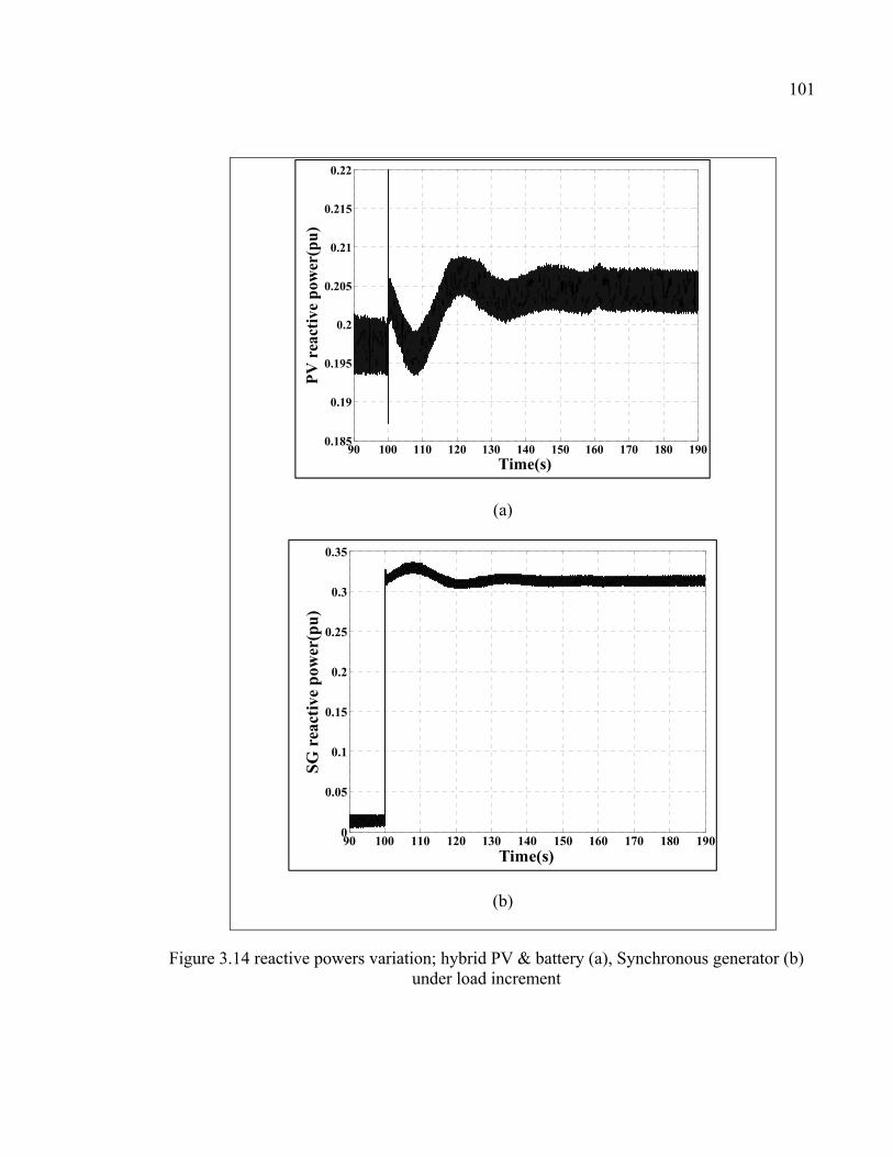
101
(a)
(b)
Figure 3.14 reactive powers variation; hybrid PV & battery (a), Synchronous generator (b) under load increment
90 100 110 120 130 140 150 160 170 180 1900.185
0.19
0.195
0.2
0.205
0.21
0.215
0.22
Time(s)
PV
rea
ctiv
e p
ower
(pu
)
90 100 110 120 130 140 150 160 170 180 1900
0.05
0.1
0.15
0.2
0.25
0.3
0.35
Time(s)
SG
rea
ctiv
e p
ower
(pu
)

102
The generators (PV and SG) increase their output power, both active and reactive power to
support the load active and reactive power increment respectively (see Figure 3.13 and
Figure 3.14). This guarantees the power sharing between different generators.
Figure 3.15 confirms that the frequency is regulated during the increment of load power at
time 100s. Figure 3.15 shows that the frequency starts to deviate after load disturbance at
time 100 s but it maintains at its nominal set point by contribution of active power (see
Figure 3.13) from both PV and SG. Therefore this test shows that PV generator participates
into frequency regulation as that of synchronous generator.
Figure 3.16 shows the droop control output p* which modifies the power reference of the
power control module. It is seen that the small frequency variation is neglected by zero
droop. Larger variation is augmented and added to the power reference. Figure 3.17 indicates
that control efforts vd and vq are bounded during this scenario (load step up).
Figure 3.18 shows the current id and iq during the increase in load power to participate in
active and reactive power regulation. Figure 3.19 shows the total dc current by PV-battery
generator is increased to support frequency and voltage regulation. The energy balance at dc
link is observed in figure 3.20(a). The control effort s2 shown in Figure 3.20(b) is bounded
during the disturbance.

103
Figure 3.15 Frequency performance
Figure 3.16 Droop performance p*
80 100 120 140 160 1800.96
0.965
0.97
0.975
0.98
0.985
0.99
0.995
1
1.005
Time(s)
Fre
qu
ency
(pu
)
60 80 100 120 140 160 180-1
-0.5
0
0.5
1
1.5
2
2.5
3
3.5
4
Time(s)
p*

104
(a)
(b)
Figure 3.17 Control effort during load step up (a) vd (b) vq
90 100 110 120 130 140 150 160 170 180 190-0.85
-0.84
-0.83
-0.82
-0.81
-0.8
-0.79
-0.78
Time(s)
v d
90 100 110 120 130 140 150 160 170 180 1900.5
0.55
0.6
0.65
0.7
0.75
0.8
0.85
0.9
0.95
Time(s)
v q
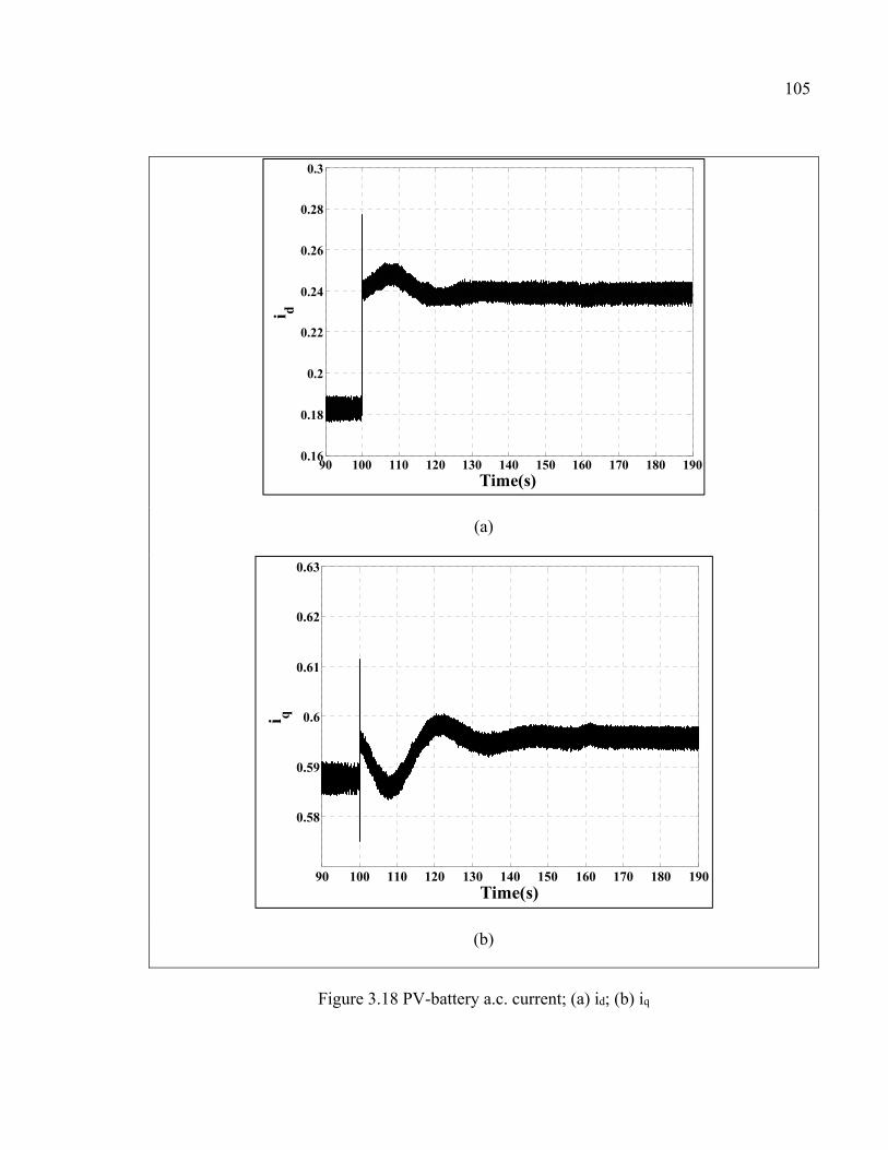
105
(a)
(b)
Figure 3.18 PV-battery a.c. current; (a) id; (b) iq
90 100 110 120 130 140 150 160 170 180 1900.16
0.18
0.2
0.22
0.24
0.26
0.28
0.3
Time(s)
i d
90 100 110 120 130 140 150 160 170 180 190
0.58
0.59
0.6
0.61
0.62
0.63
Time(s)
i q

106
Figure 3.19 PV-battery d.c. current
In addition, to test the PV performance in tracking the efficient power (maximum power
point tracking, MPPT) an insolation step change is applied to the system (1000w/m2 to
600w/m2) at times 96s and (600w/m2 to 1000w/m2) 96.5s. The PV power is tracked as shown
in Figure 3.21 (a) under applied insolation scenario. Figure 3.21 (b) shows the tracking of PV
voltage vpv. Small oscillation is seen on the tracking power due to the drawback of P&O
MPPT during fast insolation changes.
Figure 3.21 (c) demonstrates that the battery power compensates the load power under PV
power changes. The load power sharing is therefore provided by both PV-battery power even
under insolation changes.
90 100 110 120 130 140 150 160 170 180 1900.75
0.8
0.85
0.9
0.95
1
1.05
1.1
1.15
1.2
Time(s)
PV
an
d b
atte
ry c
urr
ent(
pu
)

107
(a)
(b)
Figure 3.20 Energy performance under load change (a) EDC; (b) s2
80 90 100 110 120 130 140 1500.9
0.92
0.94
0.96
0.98
1
1.02
Time(s)
En
ergy
at
DC
lin
k, E
DC
(p
u)
80 90 100 110 120 130 140 1500.218
0.22
0.222
0.224
0.226
0.228
0.23
Time(s)
s 2

108
(a)
(b)
Figure 3.21 MPPT algorithm performance; (a) PV power; (b) PV voltage
95 95.5 96 96.5 97 97.5 98 98.5 990.7
0.75
0.8
0.85
0.9
0.95
1
1.05
Time(s)
pp
v
95 95.5 96 96.5 97 97.50.8
0.85
0.9
0.95
1
1.05
1.1
1.15
1.2
Time(s)
v pv

109
(c)
Figure 3.21 MPPT algorithm performance; (c) battery power
Table 3.1 MG parameters used for simulation
MG Parameters Value
PV terminal capacitor, Cpv 590
Battery terminal capacitor, Cbat 590
DC link capacitor, CDC 1320
Boost converter inductance, L1 1
Battery boost converter inductance, L2 1
Filtering inductance, Lf 1
Nominal frequency, fn 60
Switching frequency, fsw 10
95 95.5 96 96.5 97 97.5-1.2
-1
-0.8
-0.6
-0.4
-0.2
0
0.2
0.4
Time(s)
pb
at

110
Microgrid rated power, Pn 540 W
Microgrid rated voltage, Vn 120 V
STC PV power rating, PMPP 140 W
Speed governor gain, k 0.0017
AVR gain 0.0011
100
5000
10000
1100
10000
1000
3.4 Conclusion
This chapter proposed an islanded microgrid consisting of a PV array, a battery storage and a
synchronous generator. A classical cascaded control approach based on backstepping control
with a group of cascaded control loops was proposed in order for the microgrid to participate
into: (i) voltage and frequency support, (ii) battery control and (iii) PV control. A classical
droop characteristics are suggested for frequency regulation along with the active power
control. The charging or discharging is made by implementing a simple algorithm based on
the state of the PV and load power. In addition an efficient load sharing was guaranteed. The
microgrid was validated using simulation with different scenarios such as static load power
variation (both active and reactive power) as well as insolation changes. The results show
good performance of proposed controller in frequency and voltage control.
CHAPTER 4
NONLINEAR CONTROL OF MICROGRID
4.1 Introduction
This chapter presents the design and implementation of a unified multivariable nonlinear
controller for a hybrid PV/battery system in a microgrid with two sources, as shown in Figure
4.1 consisting of a hybrid photovoltaic-battery source and a conventional synchronous
generator, equipped with its own Automatic Voltage Regulator (AVR) and speed governor.
This nonlinear controller (i.e. exact input-output feedback linearization) is designed using the
exact nonlinear model suggested in chapter 2. The main contributions of the suggested
nonlinear controller are to ensure high performance voltage and frequency regulation in the
presence of fluctuations and load variations and to integrate a conventional MPPT to enable
the PV to operate at its maximum power point. As a result of the proposed control strategy, it
is possible to use the PV-battery system to emulate a conventional synchronous generator
while automatically managing power sharing between the different units in the MG. This
feature minimizes the costs and problems associated with the presence of rotating machines.
The chapter is structured as follows: firstly the control design is presented in terms of
decoupling and linearizing control laws along with the stabilizing linear control laws. It is
followed by simulation studies. Finally, the experimental validations are presented and
discussed.
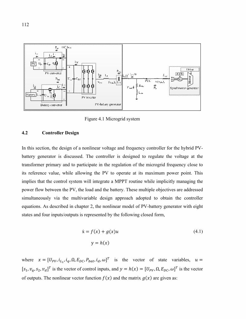
112
2S
infL
Figure 4.1 Microgrid system
4.2 Controller Design
In this section, the design of a nonlinear voltage and frequency controller for the hybrid PV-
battery generator is discussed. The controller is designed to regulate the voltage at the
transformer primary and to participate in the regulation of the microgrid frequency close to
its reference value, while allowing the PV to operate at its maximum power point. This
implies that the control system will integrate a MPPT routine while implicitly managing the
power flow between the PV, the load and the battery. These multiple objectives are addressed
simultaneously via the multivariable design approach adopted to obtain the controller
equations. As described in chapter 2, the nonlinear model of PV-battery generator with eight
states and four inputs/outputs is represented by the following closed form,
x = ( ) + ( ) y = ℎ( ) (4.1)
where = [ , , , Ω, , , , ] is the vector of state variables, =[ , , , ] is the vector of control inputs, and = ℎ( ) = [ , Ω, , ] is the vector
of outputs. The nonlinear vector function ( ) and the matrix ( ) are given as:
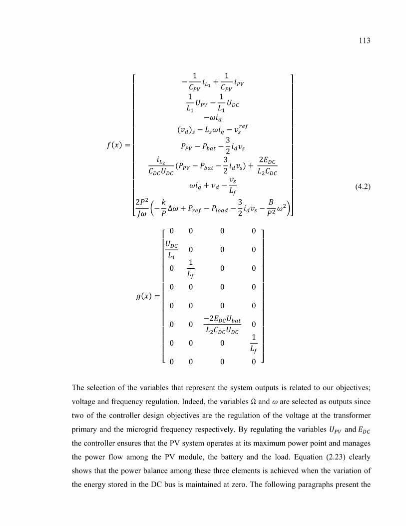
113
( ) =
− 1 + 11 − 1−( ) − −− − 32( − − 32 ) + 2+ −2 − ∆ + − − 32 −
( ) =
0000000
00 100000
00000−200
000000 10
(4.2)
The selection of the variables that represent the system outputs is related to our objectives;
voltage and frequency regulation. Indeed, the variables Ω and are selected as outputs since
two of the controller design objectives are the regulation of the voltage at the transformer
primary and the microgrid frequency respectively. By regulating the variables and
the controller ensures that the PV system operates at its maximum power point and manages
the power flow among the PV module, the battery and the load. Equation (2.23) clearly
shows that the power balance among these three elements is achieved when the variation of
the energy stored in the DC bus is maintained at zero. The following paragraphs present the

114
different steps used to obtain the controller equations using the input-output feedback
linearization technique. This method consists of a change of coordinates and a nonlinear
feedback control law to cancel system nonlinearities, in order to obtain a linear system that
will be mathematically equivalent to (4.1).
4.2.1 Decoupling and Linearizing Control Law
The dynamics of the system outputs are obtained by differentiating each output until at least
one of the inputs appears explicitly in the expression. Differentiating twice the first output
which is the PV voltage ( = ) yields the following equation,
= ( ) + ( ) (4.3)
where ( ) and ( ) are given in Table 4.1. The second output( = Ω), which was
selected to achieve the objective of terminal voltage regulation, is now differentiated until
one input appears in the expression. This gives the following equation,
= ( ) + ( ) (4.4)
Recall that the input signal is the Q-component of the D-Q reference frame representation
of the DC-AC converter terminal voltage. Similarly, the second derivative of the third output ( = E ) gives,
= ( ) + ( ) + ( ) (4.5)
The input signal is the D-component of the D-Q reference frame representation of the
DC-AC converter terminal voltage. The frequency dynamics are obtained to achieve the final
objective; participation in the microgrid frequency regulation. When the output ( = ω) is
differentiated until one input appears, the following equation is obtained:

115
= ( ) + ( ) + ( ) (4.6)
The input variable is the signal that will be used to control the switches of the bidirectional
DC-DC boost converter connected to the battery. Note that the expressions ( ) =( ( ), ( ), ( ), ( )) and ( ) = ( ( ), ( ), ( ), ( ), ( ), ( ))
are given in Table 4.1. The nonlinear model (4.1) is therefore equivalent to the following
form:
= ( )( )( )( ) + ( )0000( )0( )
00( )000( )( )
(4.7)
Table 4.1. The parameters of control system
1( ) = 1 1 − 1 11 − 11
2( ) = − 2 2 − ∆ + − − 32 − 22 + 2
3( ) = − 2 − − 32 − 22 − 32 − 1
4( ) = 2 2 2( + ) + 3 − ∆ +
1( ) = 1 2( ) = − 31( ) = 22
32( ) = −32 − − 32 − 2 2 − − 32 − − 32 2 2
41( ) = 3 2 42( ) = −3 2

116
Equation (4.7) shows the nonlinear and coupled nature of the PV/battery generator's input-
output dynamics. Applying linear control directly to this model without cancelling the system
nonlinearities, as traditionally done in the literature, may result in unsatisfactory steady state
and transient performances, in general. The control laws, which are used to cancel the system
nonlinearities while decoupling the model dynamics, have the following expression:
= ( )0000( )0( )
00( )000( )( )
− ( )− ( )− ( )− ( )
(4.8)
Note that the inverse of the above-mentioned matrix exists as long as its determinant ( ( ) ( ) ( ) ( )) is nonzero or, in other words, when the frequency and voltages
are nonzero. This is indeed the case in any range of operation. This determinant may become
zero when a short circuit occurs at the AC bus( = 0, ( ) = 0). In this case, the input
will be equal to the saturating value = [ , , , ] . For the protection
of inverter under short-circuit fault the gating signals are reset to zero. The vector =( , , , ) is representing the new input that will be used to stabilize the following
decoupled linear system, obtained when (4.8) is substituted in (4.7):
Ω = [ ] (4.9)
It can therefore be concluded that the cancellation of the nonlinear terms relating the old
inputs to the outputs by the nonlinear control law (4.8) has transformed the MIMO
PV/battery generator model into four Single-Input Single-Output (SISO) decoupled linear
systems. This model-based approach provides a systematic approach for obtaining the
controller equations using well known control design methods. The next step of the design is
to obtain the expressions for the new input signals , , , .

117
Remark I: Note that the order of the exactly linearized system (4.9) is 8, which is equal to
the order of the original nonlinear model (4.1). It can therefore be concluded that there are no
hidden internal dynamics.
Remark II: According to (4.8), the controller output signals are continuous-time signals
since they depend on state variables that are continuous-time signals. PWM modules are used
to convert these controller output signals into binary (ON and OFF) signals that are
appropriate to drive the converter switches. This is illustrated in figure 4.2. It is common to
say that controller output signals represent the switches' duty cycles.
Figure 4.2 Exact input-output feedback linearization scheme.
4.2.2 Design of the Stabilizing Linear Control Laws
The following linear expressions are proposed for the stabilizing auxiliary inputs, so that the
output = ( ,Ω, , ) tracks the reference signal = ( , Ω , , ) ,

118
= + + = + + Ω = + + = + + ω
(4.10)
where = − , = Ω − Ω, = − and = ω −ω. , Ω , and
are the reference signals of the PV terminal voltage, which are determined by the MPPT
module, the terminal voltage deviation, the energy stored in the DC bus capacitor ( ) and the angular frequency, respectively. The is the DC bus voltage
reference signal. Note that the references are constant in this application. The controller gains ( = 1,… ,4; = 1,2) are judiciously selected in such a way that the four characteristic
polynomials of the decoupled linear systems obtained when (4.10) is substituted in (4.9) are
Hurwitz polynomials, i.e.
Δ ( ) = + + = 1,… ,4
(4.11)
This ensures that the tracking errors converge to zero. The controller gains and are
tuned in order to obtain good dynamic performance. Considering the desired characteristic
polynomial of the second-order system as,
Δ ( ) = + 2 + (4.12)
and given natural frequency and damping ratio , one can calculate the controller gains so
that,
Δ ( ) = Δ ( ) (4.13)

119
This results into:
= = 2
(4.14)
As mentioned in Equation (4.9), the nonlinear system is converted into four decoupled linear
systems with transfer functions written as,
( ) = 1
(4.15)
Remark III: In practice, it is not necessary to differentiate the output variables in the
implementation of (4.10). For instance, the derivative of is implemented by taking the
right-hand side of the dynamics,
= − 1 + 1
(4.16)
4.3 Simulation Results and Discussion
In this section, the proposed voltage and frequency controller for the PV-battery generator is
first evaluated through simulation. The PV panel, battery, DC-DC converters, DC-AC
converter, transformer, load and synchronous generator illustrated in Figure 4.1 are
represented in Matlab-Simulink using SimPowerSystems blockset elements. Table 4.3
summarizes the microgrid specifications. The PV panel maximum power is 140W at
1000W/m2 with a cell temperature of 25.
The nonlinear controller, AVR and speed governor for the synchronous generator are
implemented using Matlab-Simulink elements. The nonlinear controller gains are obtained as

120
=105, =1100. These characteristics guarantee asymptotical stability and good transient
performance to the system. The PV-battery controller gains, along with the AVR and speed
governor parameters, are summarized in Table 4.3.
Two case studies are considered to evaluate the functionality of the proposed controller.
First, the frequency and voltage regulation capability is evaluated when the microgrid
operates in islanded mode. Next, the power sharing capability is tested and discussed.
4.3.1 Frequency and Voltage Regulation in MG Islanding
The following scenario is used to evaluate the frequency and voltage regulation capability of
the PV-battery generator. The microgrid operates in an islanded mode, and the active and
reactive power demands are changed abruptly at time t = 100 s. In Figures 4.3 through 4.7,
the simulation results are illustrated in per unit (p.u.) using a base power of 440 W and a base
voltage of 120 V. The active and reactive powers are increased by 0.2 p.u. respectively.
Figure 4.3 shows that the frequency begins to deviate at time t = 100 s due to the load
change, but is regulated at its rated value because of the frequency support from both
generators. Figure 4.4 shows that the voltage at the transformer secondary is regulated at its
rated value. Figure 4.5 (a,b) shows the active power sharing between the PV-battery
generator and the synchronous generator respectively. One can notice that the PV-battery
generator provides 0.1 pu of the demanded active power, increasing to 0.147 p.u. to
participate in load active power sharing. Similarly, the SG provides 0.04 p.u. and 0.19 p.u.,
respectively, before and after the load perturbation occurs. Simulation results therefore show
that the PV-battery generator and SG achieve active power participation rates of 25% and
75%, respectively. Figure 4.6 (a,b) shows the reactive power sharing between the PV-battery
generator and the synchronous generator respectively. One can notice that the PV-battery
generator provides 0.15 pu of the demanded reactive power, increasing to 0.19 p.u. to
participate in load reactive power sharing. Similarly, the SG provides 0.05 p.u. and 0.26 p.u.,
respectively, before and after the load perturbation occurs. Simulation results therefore show
that the PV-battery generator and SG achieve reactive power participation rates of 16% and

121
84%, respectively. This confirms that the PV generator behaves like a conventional generator
with a droop characteristic. Control signals vd and vq, shown in Figure 4.7, are bounded. The
d-q currents id and iq increase to provide the required active and reactive power by load as
shown in Figure 4.8.
Figure 4.3 Simulation results of microgrid frequency (p.u.)
Figure 4.4 Simulation results of microgrid terminal voltage
80 100 120 140 160 1800.97
0.975
0.98
0.985
0.99
0.995
1
1.005
Time(s)
Fre
qu
ency
(pu
)
99.8 100 100.2 100.4 100.6 100.80.975
0.98
0.985
0.99
0.995
1
1.005
1.01
1.015
Time(s)
AC
bu
s vo
ltag
e(p
u)

122
(a)
(b)
Figure 4.5 Simulation results in MG islanding mode, active power sharing (a) PV active
power, (b) SG active power
90 100 110 120 130 140 150 160 170 1800.09
0.1
0.11
0.12
0.13
0.14
0.15
0.16
0.17
Time(s)
PV
act
ive
pow
er(p
u)
90 100 110 120 130 140 150 160 170 1800
0.05
0.1
0.15
0.2
0.25
Time(s)
SG
act
ive
pow
er(p
u)

123
(a)
(b)
Figure 4.6 Simulation results in MG islanding mode, reactive power sharing (a) PV reactive
power, (b) SG reactive power
90 100 110 120 130 140 150 160 170 1800.1
0.15
0.2
0.25
Time(s)
PV
rea
ctiv
e p
ower
(pu
)
90 100 110 120 130 140 150 160 170 180-0.05
0
0.05
0.1
0.15
0.2
0.25
0.3
0.35
0.4
Time(s)
SG
rea
ctiv
e p
ower
(pu
)

124
(a)
(b)
Figure 4.7 Simulation results in MG islanding mode, (a) Control action signal, vd , (b) Control action signal, vq
90 100 110 120 130 140 150 160 170 180 190-0.92
-0.91
-0.9
-0.89
-0.88
-0.87
-0.86
-0.85
-0.84
-0.83
-0.82
Time(s)
Vd
90 100 110 120 130 140 150 160 170 1800.5
0.55
0.6
0.65
0.7
0.75
0.8
0.85
0.9
0.95
1
Time(s)
Vq

125
(a)
(b)
Figure 4.8 Simulation results in MG islanding mode, (a) d-axis current, id , (b) q-axis current, iq
100 110 120 130 140 150 1600.2
0.22
0.24
0.26
0.28
0.3
0.32
0.34
Time(s)
i d
90 100 110 120 130 140 150 1600.52
0.54
0.56
0.58
0.6
0.62
0.64
0.66
Time(s)
i q

126
4.3.2 Power Sharing Capabilities
The capability of the proposed control strategy to ensure adequate power sharing among
different components of the microgrid is tested in this section. Two different test scenarios
are used. In the first test, the insolation is changed linearly. The initial insolation is
1000W/m2. At time t = 12 s, the insolation is smoothly decreased from 1000W/m2 to
800W/m2, returning to 1000W/m2 at t = 14 s. Simulation results shown in Figure 4.9
represent the PV power, current and voltage. They demonstrate that the perturbation and
observation (P&O) technique used for the MPPT controller can quickly and accurately track
the maximum operating point of the PV panel. Figure 4.10 illustrates the control signal s1,
which is bounded. Figure 4.11 clearly shows that the battery output power is affected by the
PV power variation.
Figure 4.9 Simulation results of PV maximum power point tracking performance, PV MPPT test under insolation ramp changes, p.u.

127
Figure 4.10 Simulation results of PV maximum power point tracking performance, control action signal, s1 during insolation ramp changes, p.u.
Figure 4.11 Simulation results of PV maximum power point tracking performance, battery power during insolation ramp changes, p.u.
4.4 Experimental Validation
The nonlinear controller is now evaluated experimentally. Figure 4.12 illustrates the
microgrid setup developed in the laboratory. It includes a PV array emulator, a lead-acid
battery pack, a bidirectional DC-DC converter, a unidirectional DC-DC converter, a DC-AC
converter, AC transformers, a synchronous generator, a three-phase load and a four-pole
squirrel cage induction motor. The motor is used to supply the mechanical power required by
the synchronous generator. The induction motor is controlled by the ABB motor drive. The

128
Synchronous Generator (SG) consists of a 4-pole machine rated at 2 kW. Each phase of the
stator winding is accessible via the connection module to allow wye or delta connections.
The rotor winding is connected to two slip rings for external connection to a dc power
source. A squirrel cage damper winding is inserted in the salient-pole rotor to produce
induction-motor action, making the synchronous motor self-starting. The synchronous
generator specification is given in Table 4.2. The solar photovoltaic array consists of 5 panels
in series and 40 panels in parallel. The open circuit voltage of each panel is 9.7V and the
short circuit current is 106mA at 1000W/m2. The PV-battery controller is implemented in a
Texas Instruments TMS320F28335 digital microcontroller. The switching frequency is 10
kHz. The microgrid parameter values for this experimental setup are given in Table 4.3. A
three-phase breaker and the three-lamp method are used to synchronize the PV-battery
generator and synchronous generator. Figure 4.13 shows the AC bus voltage before and after
the synchronization.
Figure 4.12 Hardware setup of MG system

129
Table 4.2. The synchronous generator specifications
Parameters Value
Line voltage 120/208V 60 Hz
Power 1.5 kVA
Speed 1800 r/min
Current 4.2A-AC
Exciter current 0.9 A-DC
Torque 10.6 N.m
Efficiency 79 %
Friction and windage losses 150 W
Iron losses 125 W
Resistance Per Phase At 25°C (77°F)
Stator 0.6 Ω
Rotor 81 Ω
Synchronous Reactance 18.5 Ω
Exciter Inductance 6 H
Physical Characteristics
Moment of Inertia 0.097 kg·m²
Dimensions (H x W x D) 830 x 400 x 605 mm
Net Weight 89 kg
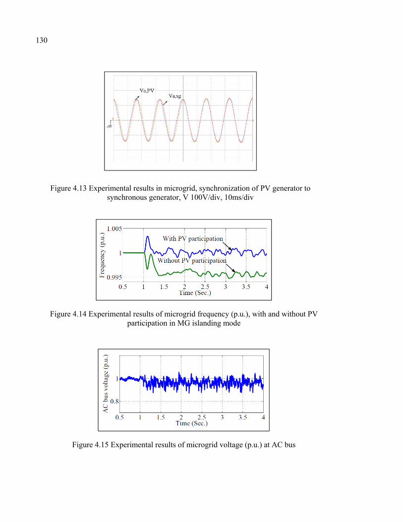
130
Figure 4.13 Experimental results in microgrid, synchronization of PV generator to synchronous generator, V 100V/div, 10ms/div
Figure 4.14 Experimental results of microgrid frequency (p.u.), with and without PV participation in MG islanding mode
Figure 4.15 Experimental results of microgrid voltage (p.u.) at AC bus

131
Figure 4.16 Experimental results, PV/battery generator ac power, p.u.
Figure 4.17 Experimental results, synchronous generator ac power, p.u.
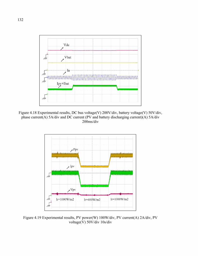
132
Figure 4.18 Experimental results, DC bus voltage(V) 200V/div, battery voltage(V) 50V/div, phase current(A) 5A/div and DC current (PV and battery discharging current)(A) 5A/div
200ms/div
Figure 4.19 Experimental results, PV power(W) 100W/div, PV current(A) 2A/div, PV voltage(V) 50V/div 10s/div

133
A load step change of 0.38 p.u. is applied to the microgrid at the time instant t = 1 s. Figure
4.14 illustrates frequency profiles when the PV-battery is both contributing and not
contributing to the system frequency regulation. It is evident that when the PV-battery
generator controller is used, the frequency steady state error is smaller. The PV/battery
generator therefore improves the frequency profile in steady state. Figure 4.15 demonstrates
that the line voltage at the AC bus is regulated at its nominal value 1 p.u. Figures 4.16 and
4.17 show that the output power of both the PV-battery generator and the synchronous
generator increase simultaneously when the load increases. This clearly demonstrates that
both generators exhibit the same behavior. Figure 4.18 represents the DC current waveform,
which is the sum of the PV current and the battery current. It should be noted that this current
increases when the load power increases. As a consequence, the AC current increases while
the DC bus voltage is regulated at its reference value. These experimental results demonstrate
both the effectiveness and robustness of the proposed model-based nonlinear controller.
Indeed, the system remains stable in spite of changes in MG parameters, such as load power.
Moreover, estimated values for the synchronous generator inertia and speed regulator gains
are used during this experimentation.
The power sharing capability of the proposed controller is also evaluated experimentally. The
PV insolation is changed linearly from 1000W/m2 to 400W/m2 and back to 1000W/m2. The
PV power, the voltage and current waveforms are shown in Figure 4.19. These results clearly
demonstrate the MPPT controller ability to track the maximum PV output power while
adequately managing the power share in the PV-battery generator when the latter contributes
to microgrid frequency and voltage support.

134
Table 4.3. The parameters of microgrid system
MG Parameters Value
PV terminal capacitor, Cpv 590
Battery terminal capacitor, Cbat 590
DC link capacitor, CDC 1320
Boost converter inductance, L1 1
Battery boost converter inductance, L2 1
Filtering inductance, Lf 1
Nominal frequency, fn 60
Switching frequency, fsw 10
Microgrid rated power, Pn 540 W
Microgrid rated voltage, Vn 120 V
STC PV power rating, PMPP 140 W
Controller proportional gain, ki1 25000
Controller derivative gain, ki2 1100
Speed governor gain, k 0.0017
AVR gain 0.0011

135
4.5 Conclusion
This chapter proposes a nonlinear voltage and frequency regulator for a hybrid photovoltaic
(PV)-battery generator through a model-based design approach. First, a multivariable input-
output feedback linearization controller was developed, based on a novel multivariable
nonlinear model which was suggested (see chapter 2) for the PV/battery generator, composed
of a PV panel with its unidirectional DC-DC converter, a lead-acid battery with its
bidirectional DC-DC converter and a DC-AC converter connected to a smoothing
inductance. Then, the proposed controller was evaluated through both simulation study and
hardware experimentation with a microgrid consisting of a PV-battery generator and a
synchronous generator equipped with its own voltage and speed regulators. Simulation and
experimental results demonstrate that the proposed control system allows the PV-Battery
generator to behave like a conventional generator. It provides both frequency and voltage
supports to the microgrid when the load's active and reactive power increases or decreases.
Moreover, an additional module is not required to manage the power between the PV, the
battery and the load. Battery output power changes automatically when the PV power
changes with the insolation, or when the load power demand changes while maintaining the
PV at its maximum power point.

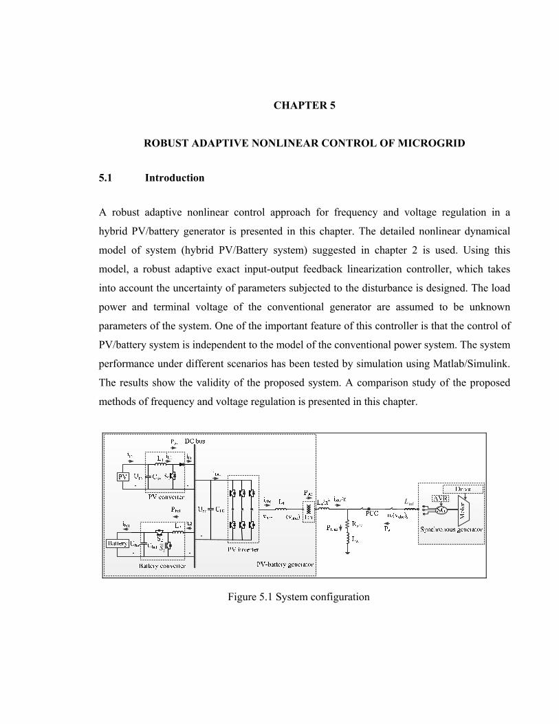
CHAPTER 5
ROBUST ADAPTIVE NONLINEAR CONTROL OF MICROGRID
5.1 Introduction
A robust adaptive nonlinear control approach for frequency and voltage regulation in a
hybrid PV/battery generator is presented in this chapter. The detailed nonlinear dynamical
model of system (hybrid PV/Battery system) suggested in chapter 2 is used. Using this
model, a robust adaptive exact input-output feedback linearization controller, which takes
into account the uncertainty of parameters subjected to the disturbance is designed. The load
power and terminal voltage of the conventional generator are assumed to be unknown
parameters of the system. One of the important feature of this controller is that the control of
PV/battery system is independent to the model of the conventional power system. The system
performance under different scenarios has been tested by simulation using Matlab/Simulink.
The results show the validity of the proposed system. A comparison study of the proposed
methods of frequency and voltage regulation is presented in this chapter.
2S
infL
Figure 5.1 System configuration

138
5.2 System configuration and modeling
To design a robust adaptive nonlinear controller for the hybrid PV/battery system, the
detailed model of system along with interfacing power electronic circuits are needed. Figure
5.1 demonstrates the structure of system suggested in this thesis that is connected to the load
and conventional diesel synchronous generator at the point of common coupling (PCC). With
no loss of generality this system can be extended to a larger scale power system network at
PCC with different sources. The complete nonlinear state-space model of 8th order is
suggested as
)(
).(),(
xhy
uxgxfx
=+= θ
(5.1)
where the vector of the state variables x , the nonlinear vector function ( , )f x θ and the
matrix ( )g x are given as,
1, , , , , , ,
T
PV L q DC bat dx U i i E P i ω = Ω
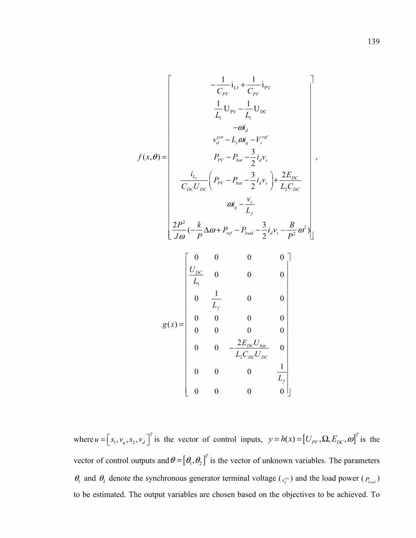
139
2
L1 PV
PV DC1 1
2
22
2
1 1i i
1 1U U
3
2
23
2
2 3( )
2
( , )
PV PV
dsyn refd s q s
PV bat d s
L DCPV bat d s
DC DC DC
sq
f
ref load d s
C C
L L
i
v L i V
P P i v
i EP P i v
C U L C
vi
L
P
f
k BP P v
x
iJ P P
ωω
ωω
θ
ω
ω
− +
−
−− −
− −
− − +
=
−
− Δ + − − −
,
1
2
0 0 0 0
0 0 0
0 0 0
0 0 0 0( )
0 0 0 0
0 0 0
0 0 0
1
0 0 0
1
0
2
DC
f
DC bat
DC DC
f
U
L
L
E U
L C U
L
g x
= −
where 1 2, , ,T
q du s v s v = is the vector of control inputs, [ ]( ) , , ,T
PV DCy h x U E ω= = Ω is the
vector of control outputs and [ ]1 2,Tθ θ θ= is the vector of unknown variables. The parameters
1θ and 2θ denote the synchronous generator terminal voltage ( syndv ) and the load power (
loadP )
to be estimated. The output variables are chosen based on the objectives to be achieved. To

140
meet the objectives of system to participate into voltage and frequency regulation, the
variables Ω and ω are chosen as outputs. On the other hand, in order to satisfy photovoltaic
optimization requirements and to manage power flow among PV, battery and loads, U and E are selected as the secondary objectives. In fact as demonstrated in chapter 2, by
minimizing the variation of reserved energy at DC bus the power balance is achieved among
these elements. The corresponding control action of system are the continuous-time signals
to generate binary signals through PWM modules for IGBT switches of power electronic
converters.
This system is nonlinear, multivariable and highly coupled with its eight state variables.
Moreover it is observed that some parameters are unknown. To handle the parameter
uncertainties subject to disturbance on the one hand, and nonlinearity on the other hand, a
systematic approach based on a robust adaptive nonlinear control strategy is designed for this
application. Next section mainly presents the design of the proposed robust adaptive exact
multivariable input-output feedback linearization for the suggested nonlinear model of PV-
battery system. The main objective of this chapter is to make the closed-loop system behave
like a conventional generator to participate into regulation of voltage as well as frequency.
The main advantages of the proposed model-based control design strategy are that these
highly coupled nonlinear dynamics will be exactly compensated. As a result, the closed-loop
system will behave exactly (and not in an approximate way around the operating point) like a
set of decoupled linear systems that can be easily controlled by linear controllers. Good
transient performances will therefore be achieved. In addition robust adaptive laws (i.e. a
direct adaptive approach) are proposed in this chapter to handle the parameter uncertainty
and disturbances in the system.
Next paragraphs demonstrate the controller design steps based on a robust adaptive exact
input-output feedback linearization technique, consisting of linearizing the nonlinear model
of Equation (5.1), and developing the robust and adaptation laws. The obtained linearized
model is decoupled and therefore a linear controller is used to stabilize the system.

141
5.3 Proposed control scheme
This section discusses the design of a robust adaptive nonlinear controller in order to satisfy
voltage and frequency regulation in the presence of nonlinearity, uncertainty and disturbance.
On the other hand voltages at the PV terminal, DC bus and AC bus need to be controlled to
their set points respectively. Additional control objectives are the regulation of system
frequency close to its nominal value, while allowing the photovoltaic system to operate at its
maximum power point (MPP) and to contribute into power sharing. The latter implies that
the control system will implicitly manage the power flow among the PV, the battery and the
load. These multiple objectives are addressed simultaneously via the proposed multivariable
design approach.
5.3.1 Decoupling and feedback linearization control laws
The dynamics of the system outputs are obtained by differentiating each output until at least
one of the inputs appears explicitly in the expression. When the input appears at the r
derivative of the output, the latter is said to have a relative degree of order r. First it is
assumed that all parameters are known.
The first objective is to control photovoltaic terminal voltage to its optimized value, namely
maximum power point voltage. This value is given by MPPT module, typically a
conventional P&O strategy (see chapter 3). Recall that the vector of state variables is =[ , , , Ω, , , , ] . The first step in the feedback linearization technique is to
apply a nonlinear change of coordinates = Τ( ). In this case the transformation is given
by:

142
)2
3(
2
2
3
11
222
2
8
7
6
5
14
3
2
1
1
ωθωω
ω
ωθ
P
Biv
P
k
J
Pz
z
ivPPz
Ez
ViLz
z
iC
iC
z
Uz
ds
dsbatPV
DC
refsqs
PVPV
LPV
pv
−−−=
=
−−=
=
−−=
Ω=
+−=
=
(5.2)
The output vector = [ , Ω, , ] is expressed in terms of the new variables as =[ , , , ] . The inverse transformation = Τ ( ) is given by:
))(2
(3
2
3
)(1
)1
(
222
2
82
7
6
5
14
3
2
1
1
ωθωω
ωω
θω
P
B
P
k
J
Pz
vP
Ji
z
ivPzP
zE
VzL
i
z
iC
zCi
zU
sd
dsPVbat
DC
refs
sq
PVPV
PVL
pv
−−−−=
=
−+−=
=
+−−=
=Ω
−−=
=
(5.3)
Differentiating the new defined state variables z until at least one of the inputs appears
considering Equation (5.2) gives,

143
dqdf
s
refs
s
s
s
s
s
s
ddsDCDC
bat
s
s
f
srefs
s
s
DCDCDC
LPV
qqf
srefs
DCDC
bat
s
s
DCPV
PVPV
DCPVPV
vvvzJL
Pv
VzL
v
L
v
P
Bz
P
kz
JP
zz
v
vdt
d
zJ
kP
P
kJzzz
P
k
z
JP
J
zP
JP
zz
P
kz
zJ
Pz
zz
vsvvszUCL
U
P
Bz
P
kz
JP
zz
v
vdt
d
L
vVz
L
v
CLz
UC
izP
dt
dz
zz
vvL
Lzz
J
P
JP
zzz
P
kVz
Jz
P
P
Bz
UCL
U
P
kz
P
Jzz
v
Lzz
zz
ssULC
idt
d
CU
LCz
LCz
zz
424147
2
14
2
227272
872
738772
2
7
227
2
287
737
2
4
8
87
322313252
22727
287
2
142
566
65
2277
2
287
71427
2
2272
27287
2714
43
111111
11
2
21
.3
)](2
3
2
3)](
/2[
2)
2([
/2]
2
/2[
4
2
32)](
/2[
2
3)(
2
3)
2()(
)2
/2)((
2
))(2
)2
((3
2
1111
2
ηης
θθθ
ηηςθ
θ
ηςθ
θθ
ης
++=−
−+−−+−−+−−−
−++−+−=
=
++=−−−−
+−−+−+−−−−=
=
+=−−+−+−−
−−−+−+=
=
+=−++−=
=
(5.4)
The vector z in terms of the outputs is given by:
×
+
=
=
d
q
v
s
v
s
z
z
z
z
y
y
y
y
2
1
4241
3231
2
1
4
3
2
1
7
5
3
1
4
3
2
1
00
00
000
000
ηηηη
ηη
ςςςς
(5.5)
Since all four inputs appear in the second derivative of respective outputs, the relative vector
of system is r = 2,2,2,2 . Since ∑ = = 8 the system is fully linearizable and there are
no zero dynamics.

144
The linearizing and decoupling control laws are obtained from (5.5). The following
expression is used to cancel the nonlinear terms that appear in (5.1).
−
=
−
4
3
2
1
4
3
2
1
1
4241
3231
2
1
2
1
00
00
000
000
ςςςς
ηηηη
ηη
v
v
v
v
v
s
v
s
d
q
(5.6)
where v = (v , v , v , v ) is the vector of auxiliary inputs that will be used to stabilize the
following decoupled linear system obtained when (5.6) is substituted in (5.5):
=
4
3
2
1
4
3
2
1
v
v
v
v
y
y
y
y
(5.7)
Therefore the cancellation of the nonlinear dynamics by the nonlinear control law (5.6) has
transformed the MIMO system model into four SISO decoupled linear systems.
The next step of the design is to obtain robust and adaptation laws for online estimation of
conventional generators’ terminal voltage and load power. In fact the uncertain parameter θ
is assumed to be unknown and subjected to disturbances. Thus a robust adaptive mechanism
is proposed to update the nonlinear controller to improve the system responses under real
situation.
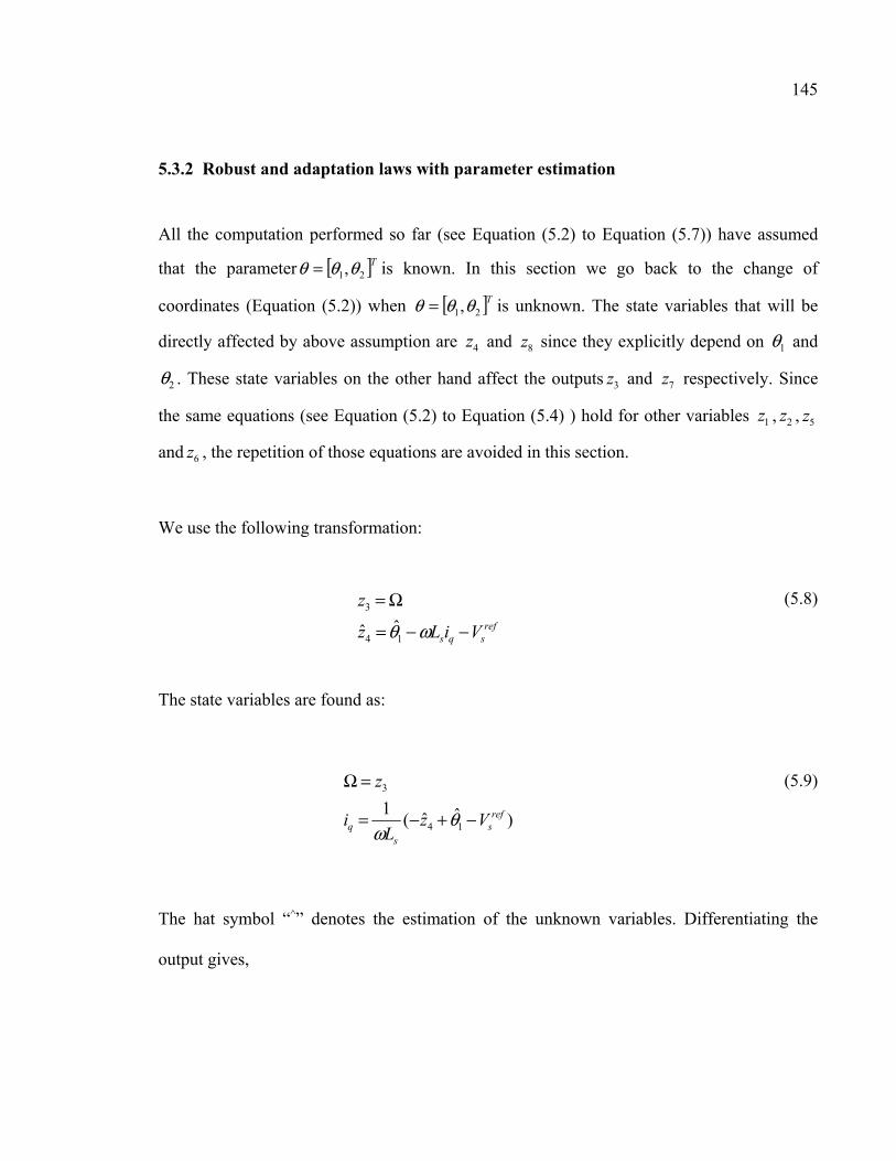
145
5.3.2 Robust and adaptation laws with parameter estimation
All the computation performed so far (see Equation (5.2) to Equation (5.7)) have assumed
that the parameter [ ]T21,θθθ = is known. In this section we go back to the change of
coordinates (Equation (5.2)) when [ ]T21,θθθ = is unknown. The state variables that will be
directly affected by above assumption are 4z and 8z since they explicitly depend on 1θ and
2θ . These state variables on the other hand affect the outputs 3z and 7z respectively. Since
the same equations (see Equation (5.2) to Equation (5.4) ) hold for other variables 1z , 2z , 5z
and 6z , the repetition of those equations are avoided in this section.
We use the following transformation:
refsqs ViLz
z
−−=
Ω=
ωθ14
3
ˆˆ
(5.8)
The state variables are found as:
)ˆˆ(1
14
3
refs
sq Vz
Li
z
−+−=
=Ω
θω
(5.9)
The hat symbol “^” denotes the estimation of the unknown variables. Differentiating the
output gives,

146
( )( )tViLViLz Nrefsqs
refsqs 111113
ˆˆ θθθωθωθ Δ++−−−=−−=Ω=
(5.10)
where θ = − and = + ∆ ( ).The equation (5.10) simplifies to,
( )tzz 1143
~ˆ θθ Δ++= (5.11)
Note that θ , and ∆ ( ) represent the estimation error, the nominal term and the small
variation of the estimated parameter respectively. Differentiating the estimated output 4z ,
one obtains:
( )
( )
qf
sdsds
qs
qsqsqs
qf
sdsds
qsNqs
qf
sdsdsqsqs
qf
dsdsqs
qsqs
vL
LiL
P
Biv
P
k
J
iLP
tJ
iLP
J
iLP
J
iLPz
vL
LiL
P
Biv
P
k
J
iLPt
J
iLPz
vL
LiL
P
Biv
P
k
J
PiL
J
PiLz
vL
iLP
Biv
P
k
J
PiLz
idt
dLiLz
ωωωωω
θω
θω
θω
θ
ωωωωωθθ
θθω
θ
ωωωωω
θω
θ
ωωωθωω
θ
ωωθ
−
+
−−−
+Δ+++=
−+
−−−
+−
Δ++=
−+
−−−+=
+−
−−−−=
−−=
222
2
2
2
2
2
2
2
14
222
2
22
222
14
222
2
2
2
14
222
2
14
14
2
32
2~2ˆ2ˆˆ
2
32ˆˆ
2ˆˆ
2
322ˆˆ
1
2
32ˆˆ
ˆˆ
(5.12)
Defining the control input qv :
+
+
−−−−−
−= 2
222
2
2
2
2
32ˆ2viL
P
Biv
P
k
J
iLP
J
iLP
L
Lv dsds
qsqs
s
fq ωωω
ωθ
ωω
(5.13)

147
the 4z is obtained as:
( )tJ
iLP
J
iLPvz qsqs
2
2
2
2
124
2~2ˆˆ θω
θω
θ Δ+++= (5.14)
Similarly we use the following transformation for the last two states:
ωθω
ω
J
Biv
J
P
J
kPz
z
ds
2
2
3ˆ22ˆ 2
2
8
7
−
+−=
=
(5.15)
The state variables are found as:
))ˆ(2
ˆ(3
222
2
82
7
ωθωω
ωω
P
B
P
k
J
Pz
vP
Ji
z
sd −−−−=
=
(5.16)
Differentiating the output 7z gives,
( )( )2222
22
2
2
7
222
2
7
ˆˆ2
2
32
)2
3(
2
θθθθω
ωωω
ωθωω
ω
+−Δ+−
−−=
−−−==
tJ
P
P
Biv
P
k
J
Pz
P
Biv
P
k
J
Pz
Nds
ds
(5.17)
where θ = − and = + ∆ ( ) one obtains:
( )tJ
P
J
Pzz 2
2
2
2
87
2~2ˆ θ
ωθ
ωΔ−−=
(5.18)

148
where θ , and ∆ ( ) represent the estimation error, the nominal term and the small
variation of the estimated parameter respectively. Differentiating the estimated output 8z ,
( )
( )
−−−
+
+
−−−−−
−−
+Δ
++
++
Δ++−−
+
−=
−−−
++
−−−−
+
−−
−−−−=
222232
4
2222
22
22
2232
4
2232
4
22
2
22
2
2
2
1
222
8
222
2
22
2
222
22
22
22
1
2
2
2
8
2
3ˆ2
3ˆ4
2
3ˆ433
2
3ˆ4~
2
3ˆ4
4~4ˆ2ˆ333ˆ
)2
3(
2
2
3ˆ2
)2
3(
223
33
2
32ˆ3ˆ2ˆ
ωθωθω
ωθωω
ωωω
θθω
θθω
θω
θω
θω
θω
ωω
ωθωω
θω
ωθωω
ω
ωωω
ωθ
ωθ
ω
P
Biv
P
kiv
J
P
P
Biv
P
k
J
BPi
J
LP
L
vi
J
vP
tivJ
Piv
J
P
tJ
BP
J
BP
J
P
J
iPvi
JL
LPv
L
v
J
Pz
P
Biv
P
k
J
Piv
J
P
P
Biv
P
k
J
P
J
Bvi
JL
LP
vL
v
J
Pi
J
LP
L
viv
J
P
J
iP
J
Pz
dsds
dsds
f
sq
s
dsds
dqd
f
sd
f
s
dsds
dsqdf
s
df
sd
s
f
sqs
d
(5.19)
Recall that qv is given in Equation (5.13). By proposing dv as:
−−−
+
+
−−−−
−
−−
−
−−=
222232
4
2222
2
222
2
42
2
3ˆ2
3ˆ4
2
3ˆ4
33
3
3
ωθωθω
ωθωω
ωωω
ωω
P
Biv
P
kiv
J
P
P
Biv
P
k
J
BP
iJ
LP
L
vi
J
vP
viJL
LPv
vP
LJv
dsds
ds
ds
f
sq
s
qdf
s
s
fd
(5.20)
the dynamics of 8z is obtained as,

149
( )tivJ
P
J
BP
ivJ
P
J
BP
J
P
J
iPvz
ds
dsd
2232
4
2
2
2232
4
2
2
2
2
1
2
48
2
3ˆ44
~
2
3ˆ44ˆ2ˆ3ˆ
θθωω
θθωω
θω
θω
Δ
+++
+++−−=
(5.21)
By defining the new variable as:
++=
−=
−=
−=
=
ds
d
qs
ivJ
P
J
BP
J
P
J
iP
J
P
J
iLP
2
3ˆ44
2
3
2
2
232
4
2
2
5
2
4
2
3
2
2
2
1
θωω
ρ
ωρ
ωρ
ωρ
ωρ
the closed loop dynamics of the entire system is formed as,
( )( )
( )( )tvz
tzz
vz
zz
tvz
tzz
vz
zz
2525241348
222287
36
65
2121124
1143
12
21
~ˆˆˆ
~ˆ
~ˆˆ
~ˆ
θρθρθρθρ
θρθρ
θρθρθ
θθ
Δ++++=
Δ++=
==
Δ+++=
Δ++=
==
(5.22)
The state-space representation is obtained as,

150
ΔΔ
+
+
+
=
)(
)(
0
0
00
00
0
01
00
00
ˆ
ˆ
00
00
00
01
00
00
00
~
~
0
0
00
00
0
01
00
00
1000
0000
0100
0000
0010
0000
0001
0000
ˆ
ˆ
00000000
10000000
00000000
00100000
00000000
00001000
00000000
00000010
ˆ
ˆ
2
1
5
2
1
2
1
43
2
1
5
2
1
4
3
2
1
8
7
6
5
4
3
2
1
8
7
6
5
4
3
2
1
t
t
v
v
v
v
z
z
z
z
z
z
z
z
z
z
z
z
z
z
z
z
θθ
ρρ
ρ
θ
θ
ρρ
θθ
ρρ
ρ
(5.23)
Considering the following general form,
z = Az + Bv + ψθ +Wθ + ψ∆θ(t) z = ( , , , z , , , , z ) , θ = θ , θ , θ = θ , θ , ∆θ(t) = (∆θ (t), ∆θ (t))
=
=
=
=
435
2
1
00
00
00
01
00
00
00
,
0
0
00
00
0
01
00
00
,
1000
0000
0100
0000
0010
0000
0001
0000
,
00000000
10000000
00000000
00100000
00000000
00001000
00000000
00000010
ρρρρ
ρψ WBA
(5.24)

151
we choose the auxiliary control input v = −Hz + p(t) where H = (h , h , h , h ) . The
Equation (5.21) is simplified to
= ( − ) + + (5.25)
The gain H is chosen so that A − BHto be Hurwitz. The term p(t) is considered into the
control Equation (5.22) to compensate the perturbation ∆θ(t) and to guarantee the robustness
in control design. The objective in this stage is to obtain the robust and adaptation laws.
Supposing A = A − BH,we define e and ε such that:
e = A e +Wθ, e(0) = 0 (5.26) ε = z − e (5.27)
whereε is the augmented error and e is the error augmentation.
It is easy to show:
ε = A ε + Bp(t) + ψθ + ψ∆θ(t) (5.28)
To determine the robust and adaptation laws, we consider the following Lyapunov candidate:
V = 12 ε Pε + 12θ Γ θ (5.29)

152
where is such that + = − , > 0 and Γ > 0. The derivation of V gives:
V = ε (A P + PA )ε + 2θ ψ Pε + 2∆θ ψ Pε + 2ε PBp(t) + 2θ Γ θ = −ε Qε + 2θ ψ Pε + Γ θ + 2∆θ ψ Pε + 2ε PBp(t) (5.30)
To find the robust and adaptation laws such that V ≤ 0,we choose θ = −θ so that the
adaptation law is obtained as:
θ = −θ = −Γψ Pε (5.31)
where Γ is the vector of positive gains. Using the following relationship,
|X Y| ≤ K4 X X + 1KY Y,X, Y ∈ ℛ , K ∈ ℛ (5.32)
Equation (5.27) is simplified to the inequality as:
V ≤ −ε Qε + 2ε PBp(t) + 1K∆θ ∆θ + Kε Pψψ Pε (5.33)
Choosing robust term p(t) as,
p(t) = −K2 B (B B) ψψ Pε (5.34)

153
the inequality in (5.33) is simplified to:
V ≤ −ε Qε + 1K∆θ ∆θ (5.35)
Bound using Bellman-Gronwall Lemma and Transition Matrix Approach:
The Lyapunov candidate Vsatisfies:
V ≤ −∝ V + 1K ( ) (5.36)
Where ∝ and ( ) are found using inequality (5.35) as
∝= 2ε Qε(ε Pε + θ Γ θ) ( ) = ∆θ ∆θ
The term ( ) is called the perturbation function of inequality (5.36). The perturbed system
with the differential Equation (5.28) is stable if
‖ ( )‖‖V‖ ≤ μ (5.37)
The solution of (5.33) is
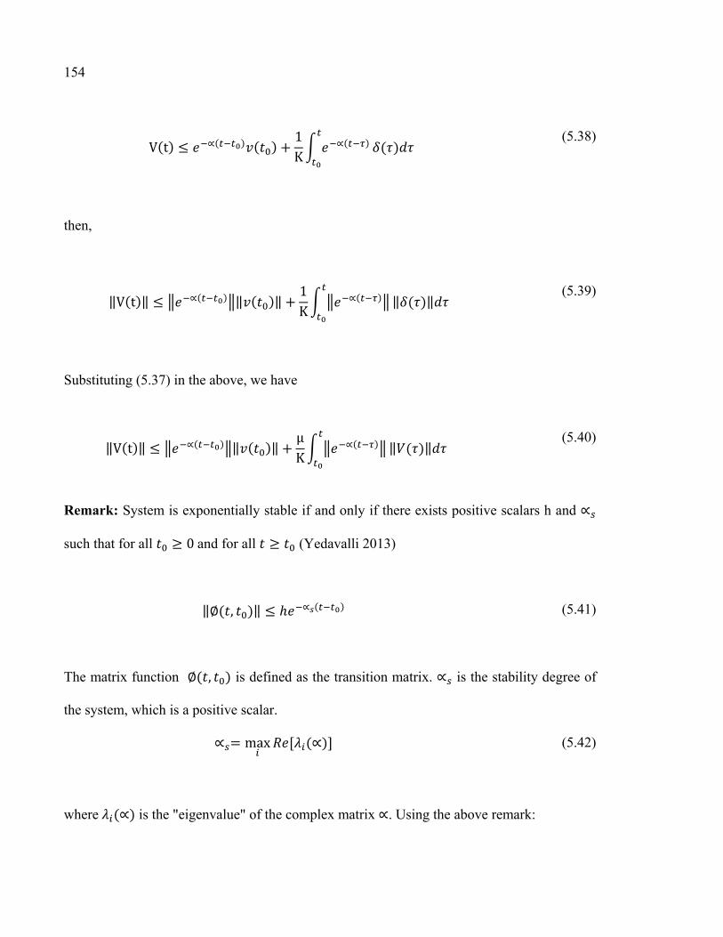
154
V(t) ≤ ∝( ) ( ) + 1K ∝( ) ( ) (5.38)
then,
‖V(t)‖ ≤ ∝( ) ‖ ( )‖ + 1K ∝( ) ‖ ( )‖ (5.39)
Substituting (5.37) in the above, we have
‖V(t)‖ ≤ ∝( ) ‖ ( )‖ + μK ∝( ) ‖ ( )‖ (5.40)
Remark: System is exponentially stable if and only if there exists positive scalars h and ∝
such that for all ≥ 0and for all ≥ (Yedavalli 2013)
‖∅( , )‖ ≤ ℎ ∝ ( ) (5.41)
The matrix function ∅( , ) is defined as the transition matrix. ∝ is the stability degree of
the system, which is a positive scalar. ∝ = max [ (∝)] (5.42)
where (∝) is the "eigenvalue" of the complex matrix ∝. Using the above remark:

155
‖V(t)‖ ≤ h ∝ ( ) ‖ ( )‖ + h. μK ∝ ( ) ‖ ( )‖ (5.43)
that is,
∝ ‖V(t)‖ ≤ h ∝ ‖ ( )‖ + h. μK ∝ ‖ ( )‖ (5.44)
Using the Bellman-Gronwall lemma, which says that when ℎ( ) ≤ + ( ) ℎ( ) then:
ℎ( ) ≤ ( ) (5.45)
with ( ) = . ,we obtain
∝ ‖V(t)‖ ≤ h ∝ ‖ ( )‖ .
(5.46) ‖V(t)‖ ≤ h ( )‖ ( )‖ (5.47)
where β =∝ − .. Choosing μ∗ = ∝
, we have that ∀μ ∈ [0, μ∗), β > 0 and therefore, V(t) → 0 exponentially fast, which implies that the equilibrium state = 0 of (5.24) is
uniformly asymptotically stable (u.a.s) in large.
The stability of the system subject to perturbations is therefore assured. The robust and
adaptation laws are therefore given as,

156
θ = Γψ Pε ε = z − e e = A e +WΓψ Pε, e(0) = 0
p(t) = K2 (B B) B ψψ Pε
(5.48)
The next step of the design is to obtain the expressions for the auxiliary signals that are the
inputs of system (5.7).
5.3.3 Design of stabilizing linear control laws
In order for the outputs to track their respective references, the following stabilizing control
inputs are suggested,
v = h (y − y ) + h (−y ) + p ( ) v = h (y − y ) + h (−y ) + p ( ) v = h (y − y ) + h (−y ) + p ( ) = ℎ ( − ) + ℎ (− ) + p ( ) (5.49)
where y1REF,y2
REF, y3REF and y4
REFare the set-points for the corresponding outputs. The term p( ) is included in (5.49) to assure the robustness of the controller. In order for the tracking
errors to converge to zero, the positive controller gains are appointed such that the
characteristic polynomials of the systems, obtained by substituting (5.49) into (5.7) are
Hurwitz. The configuration of the proposed controller is demonstrated in Figure 5.2.
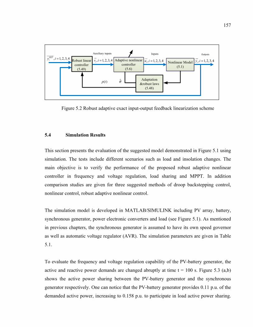
157
Nonlinear Model (5.1)
Adaptive nonlinear controller
(5.6)
, 1,2,3,4iu i =
, 1, 2,3,4iv i =, 1, 2,3,4REF
iy i =
, 1, 2,3,4iy i =
θ
Auxiliary inputs Inputs Outputs
( )p tAdaptation
&robust laws (5.48)
Robust linear controller
(5.49)
Figure 5.2 Robust adaptive exact input-output feedback linearization scheme
5.4 Simulation Results
This section presents the evaluation of the suggested model demonstrated in Figure 5.1 using
simulation. The tests include different scenarios such as load and insolation changes. The
main objective is to verify the performance of the proposed robust adaptive nonlinear
controller in frequency and voltage regulation, load sharing and MPPT. In addition
comparison studies are given for three suggested methods of droop backstepping control,
nonlinear control, robust adaptive nonlinear control.
The simulation model is developed in MATLAB/SIMULINK including PV array, battery,
synchronous generator, power electronic converters and load (see Figure 5.1). As mentioned
in previous chapters, the synchronous generator is assumed to have its own speed governor
as well as automatic voltage regulator (AVR). The simulation parameters are given in Table
5.1.
To evaluate the frequency and voltage regulation capability of the PV-battery generator, the
active and reactive power demands are changed abruptly at time t = 100 s. Figure 5.3 (a,b)
shows the active power sharing between the PV-battery generator and the synchronous
generator respectively. One can notice that the PV-battery generator provides 0.11 p.u. of the
demanded active power, increasing to 0.158 p.u. to participate in load active power sharing.

158
Similarly, the SG provides 0.03 p.u. and 0.175 p.u., respectively, before and after the load
perturbation occurs. Simulation results therefore show that the PV-battery generator and SG
achieve active power participation rates of 26.4% and 73.6%, respectively. Figure 5.4 (a,b)
shows the reactive power sharing between the PV-battery generator and the synchronous
generator respectively. One can notice that the PV-battery generator provides 0.16 p.u. of the
demanded reactive power, increasing to 0.217 p.u. to participate in load reactive power
sharing. Similarly, the SG provides 0.04 p.u. and 0.27 p.u., respectively, before and after the
load perturbation occurs. Simulation results therefore show that the PV-battery generator and
SG achieve reactive power participation rates of 19.86% and 79.04%, respectively. This
confirms that the PV generator behaves like a conventional generator with a droop
characteristic.
Figure 5.5 (a,b) shows that the SG terminal voltage and rotor speed which are considered
unknown in control design.
The d-q currents id and iq increase to provide the required active and reactive power by load
as shown in Figure 5.6. Control signals vd and vq, shown in Figure 5.7, are bounded.
Figure 5.8 confirms that the frequency is regulated during increment of load power at time
100 s. Figure 5.9 shows the regulation of the AC bus voltage. Therefore this test shows that
hybrid PV/battery generator participates into frequency and voltage regulation as that of
synchronous generator.

159
(a)
(b)
Figure 5.3 Load sharing active power; (a) PV/battery active power; (b) SG active power
90 100 110 120 130 140 150 160 170 1800.1
0.11
0.12
0.13
0.14
0.15
0.16
0.17
0.18
Time(s)
PV
act
ive
pow
er(p
u)
90 100 110 120 130 140 150 160 170 1800
0.05
0.1
0.15
0.2
0.25
Time(s)
SG
act
ive
pow
er(p
u)

160
(a)
(b)
Figure 5.4 Load sharing reactive powers; (a) PV/battery reactive power; (b) SG reactive power
90 100 110 120 130 140 150 160 170 1800.12
0.14
0.16
0.18
0.2
0.22
0.24
0.26
Time(s)
PV
rea
ctiv
e p
ower
(pu
)
90 100 110 120 130 140 150 160 170 180-0.05
0
0.05
0.1
0.15
0.2
0.25
0.3
0.35
0.4
Time(s)
SG
rea
ctiv
e p
ower
(pu
)

161
(a)
(b)
Figure 5.5 SG regulation; (a) SG terminal voltage , (b) speed regulation
99 99.5 100 100.5 101 101.5 102 102.5 1030.985
0.99
0.995
1
1.005
Time(s)
SG
ter
min
al v
olta
ge(p
u)
80 100 120 140 160 1800.97
0.975
0.98
0.985
0.99
0.995
1
1.005
1.01
Time(s)
Rot
or s
pee
d(p
u)

162
(a)
(b)
Figure 5.6 inverter current regulation; (a) id , (b) iq
100 110 120 130 140 150 1600.2
0.22
0.24
0.26
0.28
0.3
0.32
0.34
0.36
Time(s)
i d
90 100 110 120 130 140 150 1600.52
0.54
0.56
0.58
0.6
0.62
0.64
0.66
Time(s)
i q

163
(a)
(b)
Figure 5.7 Inverter control action; (a) vd , (b) vq
90 100 110 120 130 140 150 160 170 180 190-0.87
-0.86
-0.85
-0.84
-0.83
-0.82
-0.81
-0.8
-0.79
-0.78
-0.77
Time(s)
Vd
90 100 110 120 130 140 150 160 170 1800.5
0.55
0.6
0.65
0.7
0.75
0.8
0.85
0.9
0.95
1
Time(s)
Vq

164
Figure 5.8 Frequency performance
Figure 5.9 AC bus voltage performance
80 100 120 140 160 1800.97
0.975
0.98
0.985
0.99
0.995
1
1.005
Time(s)
Fre
qu
ency
(pu
)
99.8 100 100.2 100.4 100.6 100.80.985
0.99
0.995
1
1.005
Time(s)
AC
bu
s vo
ltag
e(p
u)

165
(a)
(b)
Figure 5.10 Parameter estimation; (a) 1Θ , (b) 2Θ
99.8 100 100.2 100.4 100.6 100.80.97
0.98
0.99
1
1.01
1.02
1.03
Time(s)
Est
imat
ed v
aria
ble
θ1
100 105 110 115 120 1250.16
0.18
0.2
0.22
0.24
0.26
0.28
0.3
0.32
Time(s)
Est
imat
ed v
aria
ble
θ2

166
According to robust and adaptation laws (see Equation (5.48)), the proposed controller is fed
by unknown parameters 1Θ and 2Θ . The estimation of these parameters is presented in Figure
5.10 (a) and Figure 5.10 (b) respectively. The parameter 1Θ which is the SG terminal voltage
is well estimated at its nominal value. The parameter 2Θ which is the load active power
follows the load step change discussed in previous results. Since the Direct (robust) adaptive
nonlinear controller is used, the precise estimation of unknown variables is not necessary.
The objective of the direct adaptation approach is to estimate the variable such that the
controller tracks the reference under uncertainty. Therefore these results confirm the
proposed controller performance under disturbance and uncertainty.
In addition, to test the PV performance in tracking the efficient power (maximum power
point tracking, MPPT) an insolation ramp change is applied to the system shown in Figure
5.11 (a). The PV optimal power is tracked as shown in Figure 5.12 ("a" and "b") under
applied insolation scenario.
(a)
Figure 5.11 MPPT test; (a) insolation ramp change
0.45 10 15 20 250.3
0.4
0.5
0.6
0.7
0.8
0.9
1
1.1
Time(Sec.)
Inso
lati
on(p
u)
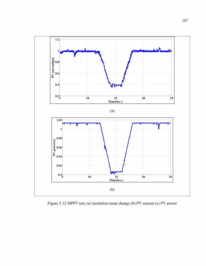
167
(a)
(b)
Figure 5.12 MPPT test; (a) insolation ramp change (b) PV current (c) PV power
5 10 15 20 250.2
0.4
0.6
0.8
1
1.2
Time(Sec.)
PV
cur
rent
(pu)
5 10 15 20 250.9
0.92
0.94
0.96
0.98
1
1.02
Time(Sec.)
PV
pow
er(w
)

168
Comparison studies of modern control vs. classical control
In this section a comparison studies are performed for three suggested methods in this thesis:
droop backstepping control, nonlinear control and robust adaptive nonlinear control. Figure
5.13 shows that the robust adaptive nonlinear control outperforms other methods in
regulation of frequency. The frequency transient is improved compared to classical control
approach. Moreover the steady state error is reduced by modern control. Figure 5.14
indicates an improvement in transient in AC bus voltage regulation using modern control
method compared to the classical control method. These improvements in frequency and
voltage regulation are resulted by accurate active and reactive power support by PV-battery
system as the exact nonlinearity of system with proper estimation of unknown parameters is
taken into account.
Figure 5.13 Frequency comparison between RANLC (Robust adaptive Nonlinear Control),
NLC ( Nonlinear Control) and classical droop control
80 100 120 140 160 1800.96
0.965
0.97
0.975
0.98
0.985
0.99
0.995
1
1.005
Time(s)
Fre
qu
ency
(pu
)
RANLCNLCDroop

169
Figure 5.14 AC bus voltage comparison between RANLC (Robust adaptive Nonlinear
Control), NLC ( Nonlinear Control) and classical control
Table 5.1. The parameters of microgrid system
MG Parameters Value
PV terminal capacitor, Cpv 590
Battery terminal capacitor, Cbat 590
DC link capacitor, CDC 1320
Boost converter inductance, L1 1
Battery boost converter inductance, L2 1
Filtering inductance, Lf 1
99.8 100 100.2 100.4 100.6 100.80.97
0.975
0.98
0.985
0.99
0.995
1
1.005
1.01
1.015
Time(s)
AC
bu
s vo
ltag
e(p
u)
RANLCNLClassic
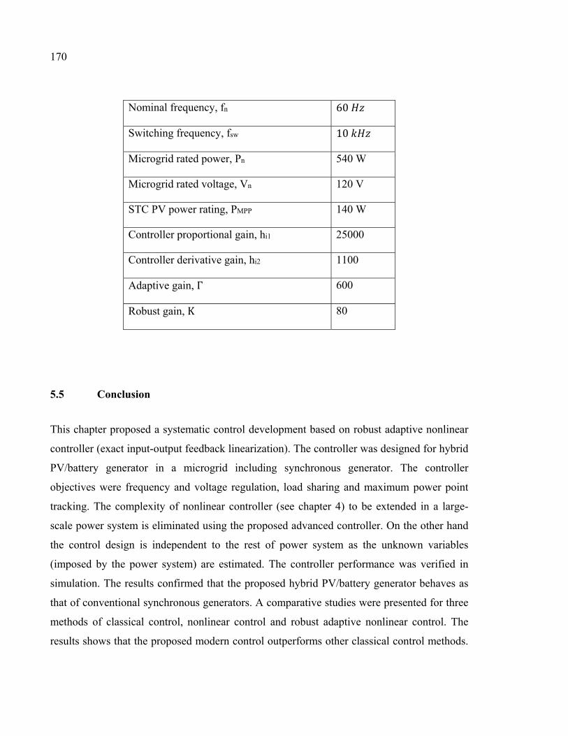
170
Nominal frequency, fn 60
Switching frequency, fsw 10
Microgrid rated power, Pn 540 W
Microgrid rated voltage, Vn 120 V
STC PV power rating, PMPP 140 W
Controller proportional gain, hi1 25000
Controller derivative gain, hi2 1100
Adaptive gain, Γ 600
Robust gain, K 80
5.5 Conclusion
This chapter proposed a systematic control development based on robust adaptive nonlinear
controller (exact input-output feedback linearization). The controller was designed for hybrid
PV/battery generator in a microgrid including synchronous generator. The controller
objectives were frequency and voltage regulation, load sharing and maximum power point
tracking. The complexity of nonlinear controller (see chapter 4) to be extended in a large-
scale power system is eliminated using the proposed advanced controller. On the other hand
the control design is independent to the rest of power system as the unknown variables
(imposed by the power system) are estimated. The controller performance was verified in
simulation. The results confirmed that the proposed hybrid PV/battery generator behaves as
that of conventional synchronous generators. A comparative studies were presented for three
methods of classical control, nonlinear control and robust adaptive nonlinear control. The
results shows that the proposed modern control outperforms other classical control methods.

CONCLUSION
Concluding Remarks:
This research thesis suggested advanced and innovative control strategies to make the PV-
battery system behave like a conventional generator e.g. synchronous generator in voltage
and frequency regulation while automatically managing power sharing between different
modules. This thesis was structured based on modeling, control design and validation using
both simulation and experimental investigation at GREPCI laboratory.
First, an accurate and nonlinear multi-input multi-output (MIMO) dynamical model of
system was extracted. This model was used for the design of a systematic control scheme i.e.
robust adaptive nonlinear control.
Second, a classical control approach consisting of a group of control loops was developed to
tackle the problem associated with frequency and voltage regulation of PV system.
Maximum power point tracking (MPPT) was integrated into the controller. While the results
confirmed that the PV system participates into the frequency and voltage regulation, the
exact system nonlinearity and parameter uncertainty were not taken into account in the
design. The control method needed a power sharing algorithm i.e. charging or discharging
battery power. A simulation was done to validate the controller performance.
Third, a systematic nonlinear voltage and frequency control strategy in which the system
nonlinearity was considered in the design was proposed (according to the proposed MIMO
model). The power sharing was automatically met in the control development. An MPPT was
integrated to extract the maximum PV power. The parameter uncertainties subjected to
disturbance were not considered in this design. The control method was validated using both
simulation and laboratory experimentation.
Fourth, an advanced and innovative voltage and frequency control strategy which is robust,
adaptive and nonlinear is proposed via nonlinear dynamics of system. These controllers are

172
designed to drive switching converters such that the perturbation, uncertainty and
nonlinearity of the system as well as power sharing by battery are taken into account in
control design. To extract the optimum power of PV generator, a maximum power point
tracking (MPPT) algorithm is integrated into the controller. The validations of the proposed
strategy were conducted in simulation. A comparison studies using simulation were
performed to show the effectiveness of the proposed modern control compared to classical
approach.
RECOMMENDATIONS
1) Due to the lack of the synchronous generator (SG) and load models in this thesis, a
primary recommendation might involve integrating the load model and the complete
model of SG (transient-saturation model) to the proposed model in chapter 2;
2) The design and implementation of robust adaptive nonlinear control using the extended
model of hybrid PV-battery-SG is recommended;
3) A model based control for parallel operation of PV inverters, their synchronization and
load sharing in a microgrid are recommended;
4) Fast islanding detection method is recommended;
5) An automatic synchronization between the PV and SG is recommended;
6) The topology of the hybrid PV/battery/SG microgrid system lacks the static transfer
switch. It is recommended to consider a static transfer switch (STS) module at the point
of common coupling (PCC);
7) The design of the control and transfer algorithm for the STS is recommended;
8) It is recommended to develop a nonlinear MPPT method which is suitable for partial
shading situation which PV characteristics impose multiple peaks;
9) It is recommended to develop a model of MG for unbalanced and dynamic loads and to
apply robust adaptive nonlinear control for these loads.


LIST OF REFERENCES
Abuzed, S. A., et al. (2014). Variable PWM step-size for modified Hill climbing MPPT PV converter. Power Electronics, Machines and Drives (PEMD 2014), 7th IET International Conference on. Afghoul, H. and F. Krim (2012). Intelligent energy management in a photovoltaic installation using neuro-fuzzy technique. Energy Conference and Exhibition (ENERGYCON), 2012 IEEE International. Ahmed, A., et al. (2012). Perturbation parameters design for hill climbing MPPT techniques. Industrial Electronics (ISIE), 2012 IEEE International Symposium on. Arboleya, P., et al. (2010). An improved control scheme based in droop characteristic for microgrid converters. Electric Power Systems Research 80(10): pp.1215-1221. Alvaro Laria, Octavian Curea, Jaime Jiménez, Haritza Camblong (2011). Survey on microgrids: Unplanned islanding and related inverter control techniques. Renewable Energy, Volume 36, Issue 8, August 2011, pp. 2052-2061, ISSN 0960-1481 Arulmurugan, R. and N. Suthanthira Vanitha (2013). Intelligent fuzzy MPPT controller using analysis of DC to DC novel buck converter for photovoltaic energy system applications. Pattern Recognition, Informatics and Mobile Engineering (PRIME), 2013 International Conference on. Åström, K. J. and B. Wittenmark (2013). Adaptive control, Courier Corporation. Au-Yeung, J., et al. (2009). Development of a voltage and frequency control strategy for an autonomous LV network with distributed generators. Universities Power Engineering Conference (UPEC), 2009 Proceedings of the 44th International, IEEE. Augustine, S., et al. (2015). Adaptive Droop Control Strategy for Load Sharing and Circulating Current Minimization in Low-Voltage Standalone DC Microgrid. Sustainable Energy, IEEE Transactions on 6(1): pp.132-141. Babazadeh, M. and H. Karimi (2011). Robust decentralized control for islanded operation of a microgrid. Power and Energy Society General Meeting, 2011 IEEE. Bakken, D. (2014). Smart Grids: Clouds, Communications, Open Source, and Automation, CRC Press. Balaguer, I. J., et al. (2011). Control for grid-connected and intentional islanding operations of distributed power generation. IEEE Transactions on Industrial Electronics, Volume 58, Issue 1, pp. 147-157.

176
Banu, I. V., et al. (2013). Comparative analysis of the perturb-and-observe and incremental conductance MPPT methods. Advanced Topics in Electrical Engineering (ATEE), 2013 8th International Symposium on. Barklund, E., et al. (2008). Energy management in autonomous microgrid using stability- constrained droop control of inverters. Power Electronics, IEEE Transactions on 23(5): pp. 2346-2352. Basso, T. S. and R. DeBlasio (2004). IEEE 1547 series of standards: interconnection issues. Power Electronics, IEEE Transactions on p. 19(5): pp.1159-1162. Baudoin, S., et al. (2012). A review of voltage and frequency control strategies for islanded microgrid. System Theory, Control and Computing (ICSTCC), 2012 16th International Conference. Bayindir, R., et al. (2015). Investigation on North American Microgrid Facility. International Journal of Renewable Energy Research (IJRER) 5(2): pp.558-574. Beehler, J. G. C. a. M. E. (2008). Implementing Smart grid communications. Burns and McDonnell Tech brief. Berridge, K. C. (2010). Robert Zajonc: The Complete Psychologist. Emot Rev 2(4): pp.348- 352. Bhatt, R. and B. Chowdhury (2011). Grid frequency and voltage support using PV systems with energy storage. North American Power Symposium (NAPS), 2011. Bidram, A., et al. (2013). Distributed Cooperative Secondary Control of Microgrids Using Feedback Linearization. Power Systems, IEEE Transactions on 28(3): pp.3462-3470. Branco, C. G., et al. (2013). Proposal of three-phase high-frequency transformer isolation UPS topologies for distributed generation applications." IEEE Transactions on Industrial Electronics, Volume 60, Issue 4, pp. 1520-1531. Chandrokar, M., et al. (1994). Control of distributed UPS systems. Power Electronics Specialists Conference, PESC'94 Record., 25th Annual IEEE. Chen, C.-L., et al. (2010). Design of parallel inverters for smooth mode transfer microgrid applications. IEEE Transactions on Power Electronics, Volume 25, Issue 1, pp. 6-15. Chen, X. and Y. Li (2014). An islanding detection algorithm for inverter-based distributed generation based on reactive power control. IEEE Transactions on Power Electronics, Volume 29, Issue 9, pp. 4672-4683.

177
Cheng, J., et al. (2012). Analysis of power decoupling mechanism for droop control with virtual inductance in a microgrid. Dianli Xitong Zidonghua(Automation of Electric Power Systems) 36(7): pp.27-32. Chenni, R., et al. (2007). A detailed modeling method for photovoltaic cells. Energy 32(9): pp.1724-1730. Chin, C. S., et al. (2011). Optimization of partially shaded PV array using fuzzy MPPT. Humanities, Science and Engineering (CHUSER), 2011 IEEE Colloquium on. Chunqing, Q., et al. (2009). Deadbeat decoupling control of three-phase photovoltaic grid- connected inverters. Mechatronics and Automation, 2009. ICMA 2009. IEEE International Conference. Daraban, S., et al. (2013). A novel global MPPT based on genetic algorithms for photovoltaic systems under the influence of partial shading. Industrial Electronics Society, IECON 2013 - 39th Annual Conference of the IEEE. Dara Jegede (2016). The world's largest photovoltaic power stations. 2016 available http://www.imeche.org/news/news-article/top-10-solar-photovoltaic-plants-in-the- world [Accessed: 22 April 2017]. Das, D. C., et al. (2011). PSO based frequency controller for wind-solar-diesel hybrid energy generation/energy storage system. Energy, Automation, and Signal (ICEAS), 2011 International Conference on, IEEE. Datta, M., et al. (2010). A voltage and frequency control approach by grid-connected MW class PV systems. Electrical Machines and Systems (ICEMS), 2010 International Conference on, IEEE. Datta, M., et al. (2011). A frequency-control approach by photovoltaic generator in a PV– diesel hybrid power system. Energy Conversion, IEEE Transactions on 26(2): pp.559-571. De Araujo Ribeiro, R. L., et al. (2012). A Robust Adaptive Control Strategy of Active Power Filters for Power-Factor Correction, Harmonic Compensation, and Balancing of Nonlinear Loads. IEEE Transactions on Power Electronics, Volume 27, Issue 2, pp. 718-730. De Brabandere, K., et al. (2007). Control of Microgrids. Power Engineering Society General Meeting, 2007. IEEE. De, D. and V. Ramanarayanan (2010). Decentralized parallel operation of inverters sharing unbalanced and nonlinear loads. Power Electronics, IEEE Transactions on 25(12): pp.3015-3025.

178
Dragicevic, T., et al. (2014). Supervisory control of an adaptive-droop regulated dc microgrid with battery management capability. Power Electronics, IEEE Transactions on 29(2): pp.695-706. Dranga, O., et al. (2004). Stability analysis of power circuit comprising virtual inductance. Circuits and Systems, 2004. ISCAS'04. Proceedings of the 2004 International Symposium on, IEEE. Ekanayake, J., et al. (2003). Control of DFIG wind turbines. Power Engineer 17(1): pp.28- 32. Elgendy, M. A., et al. (2011). Dynamic behaviour of hill-climbing MPPT algorithms at low perturbation rates. Renewable Power Generation (RPG 2011), IET Conference on. ElNozahy, M. and M. Salama (2013). Technical impacts of grid-connected photovoltaic systems on electrical networks—A review. Journal of Renewable and Sustainable Energy 5(3): pp.032702. Emadi, Ali, Abdolhosein Nasiri, and Stoyan B. Bekiarov (2004). Uninterruptible power supplies and active filters. CRC press. Eric Martinot, C. D., Liu Weiliang, and Chai Qimin (2007). Renewable Energy Future: Targets, Scenarios, and Pathways. Annual Review of Environment and Resources. Fangrui, L., et al. (2008). Comparison of P&O and hill climbing MPPT methods for grid- connected PV converter. Industrial Electronics and Applications, 2008. ICIEA 2008. 3rd IEEE Conference on. Farahani, M. (2012). Damping of subsynchronous oscillations in power system using static synchronous series compensator. Generation, Transmission & Distribution, IET 6(6): pp.539-544. Farivar, M., et al. (2011). Inverter VAR control for distribution systems with renewables. Smart Grid Communications (SmartGridComm), 2011 IEEE International Conference on. Femia, N., et al. (2004). Optimizing duty-cycle perturbation of P&O MPPT technique. Power Electronics Specialists Conference, 2004. PESC 04. 2004 IEEE 35th Annual. Femia, N., et al. (2005). Optimization of perturb and observe maximum power point tracking method. Power Electronics, IEEE Transactions on 20(4): pp.963-973. Ferreira, R. A., et al. (2013). Analysis of non-linear adaptive voltage droop control method applied to a grid connected DC microgrid. Power Electronics Conference (COBEP), 2013 Brazilian, IEEE.

179
Funato, H., et al. (2000). Transient performance of power circuit including virtual inductance realized by fully digital controlled variable active-passive reactance (VAPAR). Power Electronics Specialists Conference, 2000. PESC 00. 2000 IEEE 31st Annual, IEEE. Gayaka, S. and B. Yao (2011). Output feedback based adaptive robust fault-tolerant control for a class of uncertain nonlinear systems. Journal of Systems Engineering and Electronics, Volume 22, Issue 1, pp. 38-51. Goya, T., et al. (2011). Frequency control in isolated island by using parallel operated battery systems applying H∞ control theory based on droop characteristics. Renewable Power Generation, IET 5(2): pp.160-166. Grillo, S., et al. (2012). Optimal management strategy of a battery-based storage system to improve renewable energy integration in distribution networks. IEEE Transactions on Smart Grid, Volume 3, Issue 2, pp. 950-958. Guan-Chyun, H., et al. (2013). Photovoltaic Power-Increment-Aided Incremental- Conductance MPPT With Two-Phased Tracking. Power Electronics, IEEE Transactions on 28(6): pp. 2895-2911. Guerrero, J. M., et al. (2006). Wireless-Control Strategy for Parallel Operation of Distributed-Generation Inverters. Industrial Electronics, IEEE Transactions on 53(5): pp.1461-1470. Guerrero, J. M., et al. (2007). Decentralized control for parallel operation of distributed generation inverters using resistive output impedance. Industrial Electronics, IEEE Transactions on, 54(2): pp.994-1004. Guerrero, J. M., et al. (2011). Hierarchical Control of Droop-Controlled AC and DC Microgrids; A General Approach Toward Standardization. Industrial Electronics, IEEE Transactions on 58(1): pp.158-172. Hadji, S., et al. (2014). Experimental analysis of genetic algorithms based MPPT for PV systems. Renewable and Sustainable Energy Conference (IRSEC), 2014 International. Haruni, A., et al. (2010). Dynamic operation and control of a hybrid wind-diesel stand alone power systems. Applied Power Electronics Conference and Exposition (APEC), 2010 Twenty-Fifth Annual IEEE, IEEE. Hassouneh, M., et al. (2004). Washout filters in feedback control: Benefits, limitations and extensions. American Control Conference, 2004. Proceedings of the 2004, IEEE. Han, Hua, et al. (2016) Review of power sharing control strategies for islanding operation of AC microgrids. IEEE Transactions on Smart Grid 7.1 (2016): pp.200-215.

180
He, J. and Y. W. Li (2011). Analysis, design, and implementation of virtual impedance for power electronics interfaced distributed generation. Industry Applications, IEEE Transactions on 47(6): pp.2525-2538. Hogan, D. J., et al. (2014). Adaptive resonant current-control for active power filtering within a microgrid. Energy Conversion Congress and Exposition (ECCE), 2014 IEEE. Holland, R. A., et al. (2008). Bats use magnetite to detect the earth's magnetic field. PLoS ONE 3(2): pp. e1676, 1671-1676. Hong-Chan, C., et al. (2010). A novel electric energy management strategy applied in hybrid PV system. Power Electronics Electrical Drives Automation and Motion (SPEEDAM), 2010 International Symposium. Hu, S.-H., et al. (2011). Droop-controlled inverters with seamless transition between islanding and grid-connected operations. Energy Conversion Congress and Exposition (ECCE), 2011 IEEE, IEEE. Hua, Chihchiang, Jongrong Lin, and Chihming Shen (1998). Implementation of a DSP- controlled photovoltaic system with peak power tracking. IEEE Transactions on Industrial Electronics 45.1 (1998): 99-107. IHS (2013). PV installations in 2012 and 2013. Accessed 2016. technology.ihs.com IMS Research (2011). available http://www.pv-tech.org/news/1778 [Accessed: 2012]. Jahangiri, P. and D. C. Aliprantis (2013). Distributed Volt/VAr Control by PV Inverters. Power Systems, IEEE Transactions on 28(3): pp.3429-3439. James G. Cupp and Mike E. Beehler (2008). Implementing Smart grid communications,
Burns and McDonnell Tech brief [Online] Available: http://www.smartgridnews.com/artman/uploads/1/article-smartgrid-part2-084.pdf, [Accessed: 2012]
Jayalakshmi, N. and D. Gaonkar (2011). Performance study of isolated hybrid power system with multiple generation and energy storage units. Power and Energy Systems (ICPS), 2011 IEEE International Conference. Kakimoto, N., et al. (2009). Power modulation of photovoltaic generator for frequency control of power system. Energy Conversion, IEEE Transactions on 24(4): pp.943- 949.

181
Kaliamoorthy, M., et al. (2010). Solar powered single stage boost inverter with ANN based MPPT algorithm. Communication Control and Computing Technologies (ICCCCT), 2010 IEEE International Conference. Kanellakopoulos, I., et al. (1991). An extended direct scheme for robust adaptive nonlinear control. Automatica 27(2): pp.247-255. Karimi, H., et al. (2010). Multivariable Servomechanism Controller for Autonomous Operation of a Distributed Generation Unit: Design and Performance Evaluation. Power Systems, IEEE Transactions on 25(2): pp.853-865. Kasal, G. K. and B. Singh (2011). Voltage and frequency controllers for an asynchronous generator-based isolated wind energy conversion system. Energy Conversion, IEEE Transactions on 26(2): pp.402-416. Katiraei, F., et al. (2008). Planned islanding on rural feeders—utility perspective. Power and Energy Society General Meeting-Conversion and Delivery of Electrical Energy in the 21st Century, 2008 IEEE, IEEE. Katiraei, F., et al. (2008). Planned islanding on rural feeders; utility perspective. Power and Energy Society General Meeting - Conversion and Delivery of Electrical Energy in the 21st Century, 2008 IEEE. Katiraei, F. and M. R. Iravani (2006). Power management strategies for a microgrid with multiple distributed generation units. Power Systems, IEEE Transactions on 21(4): pp.1821-1831. Katiraei, F., et al. (2008). Microgrids management. Power and Energy Magazine, IEEE 6(3): pp.54-65. Kaufman, H., et al. (1998). Direct adaptive control algorithms: theory and applications, Springer Science & Business Media. Khaehintung, N., et al. (2006). FPGA Implementation of MPPT Using Variable Step-Size P&O Algorithm for PV Applications. Communications and Information Technologies, 2006. ISCIT '06. International Symposium on. Kim, A.-R., et al. (2013). SMES application for frequency control during islanded microgrid operation. Physica C: Superconductivity pp. 282-286. Kirubakaran, K., et al. (2011). DSP-controlled power electronic interface for fuel-cell-based distributed generation. IEEE Transactions on Power Electronics, Volume 26, Issue 2, pp. 3853-3864.

182
Kondo, Y., et al. (2010). Verification of efficacy of PSO-based MPPT for photovoltaics. Electrical Machines and Systems (ICEMS), 2010 International Conference on. Kottick, D., et al. (1993). Battery energy storage for frequency regulation in an island power system. Energy Conversion, IEEE Transactions on 8(3): pp.455-459. Krstic, M., et al. (1995). Nonlinear and adaptive control design, Wiley. Kui-Jun, L. and K. Rae-Young (2012). An adaptive maximum power point tracking scheme based on a variable scaling factor for photovoltaic systems. Vehicle Power and Propulsion Conference (VPPC), 2012 IEEE. Kui-Jun, L. and K. Rae-Young (2012). An Adaptive Maximum Power Point Tracking Scheme Based on a Variable Scaling Factor for Photovoltaic Systems. Energy Conversion, IEEE Transactions on 27(4): pp.1002-1008. Kumar, R. (2012). Dependence of hill climbing MPPT algorithm on ADC and Digital filter parameters. Power Electronics (IICPE), 2012 IEEE 5th India International Conference on. Laaksonen, H., et al. (2014). Adaptive Protection and Microgrid Control Design for Hailuoto Island. Laaksonen, H., et al. (2005). Voltage and frequency control of inverter based weak LV network microgrid. Future Power Systems, 2005 International Conference. Latif, T. and S. R. Hussain (2014). Design of a charge controller based on SEPIC and buck topology using modified Incremental Conductance MPPT. Electrical and Computer Engineering (ICECE), 2014 International Conference on. Lasseter, R. H. and P. Paigi (2004). Microgrid: a conceptual solution. Power Electronics Specialists Conference, 2004. PESC 04. 2004 IEEE 35th Annual, IEEE. Lee, C. T., et al. (2013). A New Droop Control Method for the Autonomous Operation of Distributed Energy Resource Interface Converters. Power Electronics, IEEE Transactions on 28(4): pp.1980-1993. Lee, D.-J. and L. Wang (2008). Small-signal stability analysis of an autonomous hybrid renewable energy power generation/energy storage system part I: time-domain simulations. Energy Conversion, IEEE Transactions on 23(1): pp.311-320. Lee, S.-W., et al. (2009). A tranformerless grid-connected photovoltaic system with active and reactive power control. Power Electronics and Motion Control Conference, 2009. IPEMC'09. IEEE 6th International, IEEE.

183
Lee, T.-L. and P.-T. Cheng (2007). Design of a new cooperative harmonic filtering strategy for distributed generation interface converters in an islanding network. IEEE Transactions on Power Electronics, Volume 22, Issue 5, pp. 1919-1927. Li, P., et al. (2015). Dynamic Power Conditioning Method of Microgrid Via Adaptive Inverse Control. Power Delivery, IEEE Transactions PP(99): pp.1-9. Li, X., et al. (2008). Frequency control in micro-grid power system combined with electrolyzer system and fuzzy PI controller. Journal of Power Sources 180(1): pp.468-475. Liu, S. and R. A. Dougal (2002). Dynamic multiphysics model for solar array. Energy Conversion, IEEE Transactions on 17(2): pp.285-294. Liu, X. and L. A. C. Lopes (2004). An improved perturbation and observation maximum power point tracking algorithm for PV arrays. Power Electronics Specialists Conference, 2004. PESC 04. 2004 IEEE 35th Annual. Lorenzo, E. (1994). Solar electricity: engineering of photovoltaic systems, Earthscan/James & James. Luque, A. and S. Hegedus (2011). Handbook of photovoltaic science and engineering, John Wiley & Sons. MacKunis, W., et al. (2012). Robust and adaptive maximum power point tracking for standalone photovoltaic systems using a sliding mode control approach. Industrial Electronics and Applications (ICIEA), 2012 7th IEEE Conference on. Majumder, R., et al. (2012). Power sharing and control in distributed generation with wireless sensor networks. IEEE Transactions on Smart Grid, 3(2): pp. 618-634. Mariam, L., et al. (2013). A review of existing microgrid architectures. Journal of Engineering 2013. Marino, R. and P. Tomei (1996). Nonlinear control design: geometric, adaptive and robust, Prentice Hall International (UK) Ltd. Marwali, M. N. and A. Keyhani (2004). Control of distributed generation systems-Part I: Voltages and currents control. Power Electronics, IEEE Transactions on 19(6): pp.1541-1550. Mauricio, J. M., et al. (2009). Frequency regulation contribution through variable-speed wind energy conversion systems. Power Systems, IEEE Transactions on 24(1): pp.173- 180.
184
Mengi, O. O. and I. H. Altas (2011). A fuzzy decision making energy management system for a PV/Wind renewable energy system. Innovations in Intelligent Systems and Applications (INISTA), 2011 International Symposium on. Microgrid project at Los Alamos, NM.(2015). www.losalamosnm.us [Accessed 2015]. Microgrid test-bed at Rochester Institute of Technology (RIT) New York.(2015). www.rit.edu [Accessed 2015]. Milosevic, M. and G. Andersson (2005). Generation control in small isolated power systems. Power Symposium, 2005. Proceedings of the 37th Annual North American, IEEE. Mitsubishi Electric Solar solutions. (2013). http://www.mitsubishielectricsolar.com/images/uploads/documents/specs/MLE_260 Wp_Spec_Sheet_Feb2013_lr.pdf [Accessed 2016]. Mohamed, A. A. S., et al. (2014). Optimized-fuzzy MPPT controller using GA for stand- alone photovoltaic water pumping system. Industrial Electronics Society, IECON 2014 - 40th Annual Conference of the IEEE. Mohamed, Y. A. R. I. and E. F. El-Saadany (2008). Adaptive Decentralized Droop Controller to Preserve Power Sharing Stability of Paralleled Inverters in Distributed Generation Microgrids. Power Electronics, IEEE Transactions on 23(6): pp.2806- 2816. Mohamed, Y. A. R. I. and A. A. Radwan (2011). Hierarchical Control System for Robust Microgrid Operation and Seamless Mode Transfer in Active Distribution Systems. Smart Grid, IEEE Transactions on 2(2): pp.352-362. Molina, M. and E. Espejo (2014). Modeling and simulation of grid-connected photovoltaic energy conversion systems. International Journal of Hydrogen Energy 39(16): pp.8702-8707. Moradi, R., et al. (2010). Robust decentralized control for islanded operation of two radially connected DG systems. Industrial Electronics (ISIE), 2010 IEEE International Symposium on. Nejati, A., et al. (2013). Voltage and frequency control of an islanded electronically-coupled distributed generation unit. Energy Conversion Congress and Exposition (ECCE), 2013 IEEE. Nikkhajoei, H. and R. H. Lasseter (2009). Distributed generation interface to the CERTS microgrid. IEEE Transactions on Power Delivery, 24(3): pp. 1598-1608.

185
Okou, A., et al. (2012). Nonlinear control strategy insuring contribution of PV generator to voltage and frequency regulation. Power Electronics, Machines and Drives (PEMD 2012), 6th IET International Conference on, IET. Okou, F. A., et al. (2010). A robust adaptive controller for a DFIG wind turbine with grid voltage and frequency support. Control Applications (CCA), 2010 IEEE International Conference on. Okou, F. A. and A. A. Amoussou (2008). A robust adaptive controller for a three-phase three-level neutral-point clamped rectifier. Electrical and Computer Engineering, 2008. CCECE 2008. Canadian Conference. Ota, T., et al. (2007). Study of load frequency control for a microgrid. Power Engineering Conference, 2007. AUPEC 2007. Australasian Universities, IEEE. Pachauri, R. K. and Y. K. Chauhan (2014). Hydrogen generation/pressure enhancement using FC and ANN based MPPT assisted PV system. Computational Intelligence on Power, Energy and Controls with their impact on Humanity (CIPECH), 2014 Innovative Applications of. Pappu, V. A. K., et al. (2010). Implementing frequency regulation capability in a solar photovoltaic power plant. North American Power Symposium (NAPS), 2010. Paul, S. (2013). Comparison of MPPT using GA-Optimized ANN employing PI controller with GA-Optimized ANN employing fuzzy controller for PV system. Sustainable Energy and Intelligent Systems (SEISCON 2013), IET Chennai Fourth International Conference on. Peralta, J., et al. (2009). BC Hydro perspective on distribution islanding for customer reliability improvement. Integration of Wide-Scale Renewable Resources Into the Power Delivery System, 2009 CIGRE/IEEE PES Joint Symposium. Phadke, A., et al. (1983). A new measurement technique for tracking voltage phasors, local system frequency, and rate of change of frequency. Power Apparatus and Systems, IEEE Transactions on(5): pp.1025-1038. Phan Quoc, D., et al. (2010). The new MPPT algorithm using ANN-based PV. Strategic Technology (IFOST), 2010 International Forum on. Phimmasone, V., et al. (2010). Evaluation of extracted energy from PV with PSO-based MPPT against various types of solar irradiation changes. Electrical Machines and Systems (ICEMS), 2010 International Conference on. Piagi, P. and R. H. Lasseter (2006). Autonomous control of microgrids. Power Engineering Society General Meeting, 2006. IEEE, IEEE.

186
Pogaku, N., et al. (2007). Modeling, Analysis and Testing of Autonomous Operation of an Inverter-Based Microgrid. Power Electronics, IEEE Transactions on 22(2): pp.613- 625. Pourmousavi, S., et al. (2012). Impact of high penetration of PV generation on frequency and voltage in a distribution feeder. North American Power Symposium (NAPS), 2012, IEEE. Pradhan, R. and B. Subudhi (2015). Double Integral Sliding Mode MPPT Control of a Photovoltaic System. Control Systems Technology, IEEE Transactions on PP(99): pp.1-1. Qing-Chang, Z., et al. (2014). Self-Synchronized Synchronverters: Inverters Without a Dedicated Synchronization Unit. Power Electronics, IEEE Transactions on 29(2): pp.617-630. Qing-Chang, Z. and G. Weiss (2011). Synchronverters: Inverters That Mimic Synchronous Generators. Industrial Electronics, IEEE Transactions on 58(4): pp.1259-1267. Ramaprabha, R., et al. (2011). Maximum power point tracking using GA-optimized artificial neural network for Solar PV system. Electrical Energy Systems (ICEES), 2011 1st International Conference on. Ray, P. K., et al. (2010). Dynamic modeling and control of renewable energy based hybrid system for large band wind speed variation. ISGT Europe. Rikos, E., et al. (2008). Stability and power quality issues in microgrids under weather disturbances. Selected Topics in Applied Earth Observations and Remote Sensing, IEEE Journal of 1(3): pp.170-179. Robbins, B. A., et al. (2013). A Two-Stage Distributed Architecture for Voltage Control in Power Distribution Systems. Power Systems, IEEE Transactions on 28(2): pp.1470- 1482. Roy, R. B., et al. (2014). Fuzzy logic based MPPT approach in a grid connected photovoltaic system. Software, Knowledge, Information Management and Applications (SKIMA), 2014 8th International Conference on. Saito, N., et al. (2009). Trade-off analysis of autonomous microgrid sizing with PV, diesel, and battery storage. Power & Energy Society General Meeting, 2009. PES'09. IEEE, IEEE. Salhi, I., et al. (2010). Fuzzy control of micro hydro power plants. Power Electronics, Machines and Drives (PEMD 2010), 5th IET International Conference on, IET.

187
Samadi, A., et al. (2012). Reactive Power Dynamic Assessment of a PV System in a Distribution Grid. Energy Procedia 20: pp. 98-107. Sao, C. K. and P. W. Lehn (2006). Intentional islanded operation of converter fed microgrids. Power Engineering Society General Meeting, 2006. IEEE, IEEE. Sao, C. K. and P. W. Lehn (2008). Control and Power Management of Converter Fed Microgrids. Power Systems, IEEE Transactions on 23(3): pp.1088-1098. Savaghebi, M., et al. (2012). Secondary Control Scheme for Voltage Unbalance Compensation in an Islanded Droop-Controlled Microgrid. Smart Grid, IEEE Transactions on 3(2): pp.797-807. Senjyu, T., et al. (2005). A hybrid power system using alternative energy facilities in isolated island. Energy Conversion, IEEE Transactions on 20(2): pp.406-414. Senjyu, T., et al. (2009). A control method for small utility connected large PV system to reduce frequency deviation using a minimal-order observer. Energy Conversion, IEEE Transactions on 24(2): pp. 520-528. Sera, D., et al. (2013). On the Perturb-and-Observe and Incremental Conductance MPPT Methods for PV Systems. Photovoltaics, IEEE Journal of 3(3): pp.1070-1078. Şerban, I. and C. Marinescu (2011). Aggregate load-frequency control of a wind-hydro autonomous microgrid. Renewable Energy 36(12): pp. 3345-3354. Shah, K. B. and L. P. Joshi (2013). Comparative analysis of incremental conductance base MPPT for multi-string photovoltaic system. Engineering (NUiCONE), 2013 Nirma University International Conference on. Shahgholian, G., et al. (2009). Nonlinear Control Techniques in Uninterruptible Power Supply Inverter: A Review. Computer and Electrical Engineering, 2009. ICCEE '09. Second International Conference on. Shayeghi, H., et al. (2009). Load frequency control strategies: A state-of-the-art survey for the researcher. Energy Conversion and Management 50(2): pp. 344-353. Sheraz, M. and M. A. Abido (2012). An efficient MPPT controller using differential evolution and neural network. Power and Energy (PECon), 2012 IEEE International Conference on. Shi, D., et al. (2013). Adaptive control of distributed generation for microgrid islanding. Innovative Smart Grid Technologies Europe (ISGT EUROPE), 2013 4th IEEE/PES, IEEE.
188
Siew-Chong, T., et al. (2008). Indirect Sliding Mode Control of Power Converters Via Double Integral Sliding Surface. Power Electronics, IEEE Transactions on 23(2): pp.600-611. Siew-Chong, T., et al. (2007). A Fast-Response Sliding-Mode Controller for Boost-Type Converters With a Wide Range of Operating Conditions. Industrial Electronics, IEEE Transactions on 54(6): pp.3276-3286. Sow, T., et al. (2011). Control strategy insuring contribution of DFIG-Based wind turbines to primary and secondary frequency regulation. IECON 2011 - 37th Annual Conference on IEEE Industrial Electronics Society. Sundareswaran, K., et al. (2014). MPPT of PV Systems Under Partial Shaded Conditions Through a Colony of Flashing Fireflies. Energy Conversion, IEEE Transactions on 29(2): pp. 463-472. Taheri, H., et al. (2010). A novel Maximum Power Point tracking control of photovoltaic system under partial and rapidly fluctuating shadow conditions using Differential Evolution. Industrial Electronics & Applications (ISIEA), 2010 IEEE Symposium on. Taheri, H., et al. (2013). Contribution of PV generators with energy storage to grid frequency and voltage regulation via nonlinear control techniques. Industrial Electronics Society, IECON 2013 - 39th Annual Conference of the IEEE. Taheri, H., et al. (2013). Nonlinear Frequency and Voltage Regulation in a PV-Battery- Diesel Microgrid. Eighth International Conference and Exhibition on Ecological Vehicles and Renewable Energies, Monaco. Taheri, H., et al. (2012). Contribution of Three-Phase Photovoltaic Grid-Connected Power Systems to Grid Frequency Regulation. Proceedings of the 2nd International Conference on Systems and Control, Marrakech, Morocco. Taheri, S., et al. (2012). Modified Maximum Power Point tracking (MPPT) of grid-connected PV system under partial shading conditions. Electrical & Computer Engineering (CCECE), 2012 25th IEEE Canadian Conference on. Tonkoski, R., et al. (2012). Impact of high PV penetration on voltage profiles in residential neighborhoods. Sustainable Energy, IEEE Transactions on 3(3): pp. 518-527. Tsai, H.-L., et al. (2008). Development of generalized photovoltaic model using MATLAB/SIMULINK. Proceedings of the world congress on Engineering and computer science.

189
Tuladhar, A., et al. (2000). Control of parallel inverters in distributed AC power systems with consideration of line impedance effect. Industry Applications, IEEE Transactions on. 36(1): pp.131-138. Vallvé, X., et al. (2007). Micro storage and demand side management in distributed PV grid- connected installations. Electrical Power Quality and Utilisation, 2007. EPQU 2007. 9th International Conference on, IEEE. Vasquez, J. C., et al. (2010). Hierarchical control of intelligent microgrids. Industrial Electronics Magazine, IEEE 4(4): pp.23-29. Venketraman, S., et al. (2004). Choosing a nonlinear controller for a series resonant DC-DC converter. Power Electronics Systems and Applications, 2004. Proceedings. 2004 First International Conference. Walker, G. (2001). Evaluating MPPT converter topologies using a MATLAB PV model. Journal of Electrical & Electronics Engineering, Australia 21(1): pp.49. Watson, L. D. and J. W. Kimball (2011). Frequency regulation of a microgrid using solar power. Applied Power Electronics Conference and Exposition (APEC), 2011 Twenty-Sixth Annual IEEE, IEEE. Yan, D., et al. (2011). A unified power controller for photovoltaic generators in microgrid. Electric Utility Deregulation and Restructuring and Power Technologies (DRPT), 2011 4th International Conference on, IEEE. Yan Ping, J. and L. Fang Lin (2009). An improved sliding mode controller for boost converter in solar energy system. Industrial Electronics and Applications, 2009. ICIEA 2009. 4th IEEE Conference on. Yang, F., et al. (2008). Robust Adaptive Control of Conjugated Polymer Actuators. Control Systems Technology, IEEE Transactions on 16(4): pp. 600-612. Yazdani, D., et al. (2008). A nonlinear adaptive synchronization techniquefor grid- connected distributed energy sources. Power Electronics, IEEE Transactions on 23(4): pp.2181-2186. Ye, Z., et al. (2012). Energy management strategy of islanded microgrid based on power flow control. Innovative Smart Grid Technologies (ISGT), 2012 IEEE PES. Yedavalli, R. K. (2013). Robust control of uncertain dynamic systems: a linear state space approach. Springer Science & Business Media.

190
Yuansheng, X., et al. (2012). Research on Constant Voltage with Incremental Conductance MPPT Method. Power and Energy Engineering Conference (APPEEC), 2012 Asia- Pacific. Yun Wei, L. and K. Ching-Nan (2009). An Accurate Power Control Strategy for Power- Electronics-Interfaced Distributed Generation Units Operating in a Low-Voltage Multibus Microgrid. Power Electronics, IEEE Transactions on 24(12): pp.2977- 2988. Ze, C., et al. (2011). Self-Adjusting Fuzzy MPPT PV System Control by FPGA Design. Power and Energy Engineering Conference (APPEEC), 2011 Asia-Pacific. Ze, C., et al. (2010). FPGA-based PV systems fuzzy MPPT control algorithm. Fuzzy Systems and Knowledge Discovery (FSKD), 2010 Seventh International Conference on. Zhong, Q.-C. (2010). Four-quadrant operation of AC machines powered by inverters that mimic synchronous generators. Power Electronics, Machines and Drives (PEMD 2010), 5th IET International Conference on.