RiskIArbitrage Strategies: A New Concept for AssetLiability Management, Optimal Fund Design and Optimal Portfolio Selection in a

Dynamic, Continuous-Time Framework Part 11: Securities and Derivatives Markets

Hans-Fredo List Swiss Reinsurance Company

Mythenquai 50160, CH-8022 Zurich Telephone: +411285 2351 Facsimile: +41 1 285 4179

Mark H.A. Davis Tokyo-Mitsubishi International plc 6 Broadgate, London EC2M 2AA

Telephone: +44 171 577 2714 Facsimile: +44 171 577 2888

Abstract. Assefiiability management, optimal fund design and optimal portfolio selection have been key issues of interest to the (re)insurance and investment banking communities, respectively, for some years - especially in the design of advanced risk-transfer solutions for clients in the Fortune 500 group of companies. AFIR 1996 publications dealing with these topics were, e.g., Optimal Fund Design for Investors with Holding Constraints (Vol. I , p. 245), Optimal Porlfolio and Optimal Trading in a Dynamic Continuous Time Framework (Vol. I , p. 275), Mean-Variance Portfolio Selection under Porlfolio Insurance (Vol. I , p. 347), Baseline for Exchange Rate - Risks of an International Reinsurer (Vol. I . , p. 399, Optimizing Investment and Contribution Policies of a Defined Benefit Pension Fund (Vol. I , p. 593), Continuous-Time Pension Fund Modelling (Vol. I , p. 609), Linear Approach for Solving Large-Scale Porlfolio Optimization Problems in a Lognormal Market (Vol. 11, p. 1019), Options as an Asset Class (Vol. 11, p. 1413), Optioned Porlfolios: The Trade-08 between Expected and Guaranteed Returns (Vol. 11, p. 1443), Optimal Optioned Porlfolios with Confidence Limits on Shorlfall Constraints (Vol. 11, p. 1497), among others. Taking up some of the new ideas and approaches in this literature we introduce the concept of limited risk arbitrage investment management in a general dzyusion type securities and derivatives market and characterize the corresponding trading and portfolio management strategies (risk/arbitrage strategies) as the solutions of a stochastic control problem with constraints on instantaneous investment risk, future portfolio risk dynamics, portfolio time decay dynamics and portfolio value appreciation dynamics. Part 11: Securities and Derivatives Markets shows how an efficient allocation of risk can be achieved by investing in a portfolio of securities and non-redundant (i.e., securities market completing) financial options.

Kevwords. Limited risk arbitrage investment management, instantaneous investment risk, future risk dynamics, time decay dynamics, value appreciation dynamics, risklarbitrage strategies, strategy space transformation, market parametrization, maximum principle, convex duality, Markovian characterization, market prices of risk, completion premium, target wealth, required wealth, transformation premium, canonical solution, CS (constraint set) projection, DC (drawdown control) transform.

Contents.

Part I: Securities Markets (separate paper) 1 . Introduction 2. Securities Markets, Trading and Portfolio Management

- Complete Securities Markets - Bond Markets - Stock Markets - Trading Strategies - Arrow-Debreu Prices - Admissibility - Utility Functions - Liability Funding - Asset Allocation - General Investment Management - Incomplete Securities Markets - Securities Market Completions - Maximum Principle - Convex Duality - Markovian Characterization

3. Contingent Claims and Hedging Strategies - Hedging Strategies - Mean Self-Financing Replication - Partial Replication - American Options - Market Completion With Options

Appendix: References

Part 11: Securities and Derivatives Markets 4. Derivatives Risk Exposure Assessment and Control

- Market Completion With Options - Limited Risk Arbitrage - Complete Securities Markets - Options Portfolio Characteristics - Hedging With Options

5. Riswbit rage Strategies - Limited Risk Arbitrage Investment Management - Strategy Space Transformation - Market Parametrization - Unconstrained Solutions - Maximum Principle - Convex Duality - Markovian Characterization - RiskIArbitrage Strategies - Dynamic Programming - Drawdown Control - Partid Observation

Appendix: References

4. Derivatives Risk Exposure Assessment and Control

Market Com~letion With O~tions. Recall from Parf I: Securities Markets: Within the class of general assets [i.e., assets with RCLL semimartingale price processes dV(t) = o(t)dW(t) + dA(t) where o E R , R = K(o) @ KL(o) and A(t) is of class VF (variation finie)] in the incomplete securities market model

a( t ) = ~ ( t ) ~ ~ ( t ) - ' [ ~ ( t ) - r(t)l,]

1 1 P(t) = .xP(- [ a ( s ) T d ~ ( s ) - [ lla(s)lrds) E [ ~ X P ( ~ [lla(S)lrdS)l< 0 (4.1)

S(t) = P(t)D(t) considered here contingent claims are compatible with the equilibrium bond and stock prices [i.e., after discounting with the risk-neutral discount factor D(t) their value processes are continuous martingales under the minimax local martingale measure ?ti," ] and can therefore

be written in the form

with the (partial) replication strategy 0 eKL(o) and the additional parameters w,,o, E K(o) . The first term in this representation is the value process of a purely tradable (attainable) asset while the second term characterizes a totally non-tradable asset in this financial economy. The above decomposition is unique up to constants. Furthermore, every compatible asset (with non-constant associated value process) is either purely tradable (attainable) or totally non-tradable. It also follows that the minimal equivalent martingale measure is necessarily

E(q) = E[P(H)l,], q E @ , and m(t) = W(t) + [a(s)ds (4.3)

and that any equivalent martingale measure ijj for the equilibrium security price processes is related to this minimal (in terms of its distance to the reference probability x measured in units of relative entropy) martingale measure via

[We therefore call the quantity B T v V I V V =-=bTQe

'h XVxV XVxV ' "'Yv EK(o)

a completion premium.] Moreover, among all equivalent martingale measures for the equilibrium bond and stock price processes the minimal equivalent martingale measure is characterized by the property that for every totally non-tradable asset the stochastic differential equation

dV(t) = ol(t)To,(t)dt + wl(t)TdB(t) (4.5) holds with the same coefficients w, , a , E K(o) and any (related to each other via the Girsanov theorem) x - and E - Brownian motions B(t) . Note that all the results about option

pricing and hedging derived above in the securities market completion EsyV (t) also apply in

this originally given incomplete market model 5(t) [with respect to the minimal equivalent

martingale measure it and the corresponding Girsanov transform w(t) of the exogenous sources W(t) of securities market uncertainty], i.e., we have the derivatives value processes

1 Vvc (t) = - E[D(T)C~F~ ] (European options) (4.6a)

D(t) 1

Vvc (t) = -E[D(T,)c(T,)~F~] (American options) (4.6b) D(t)

with associated risk minimizing replication costs dCVC (t) = dLc(t) , CVC (0) = VVC (0) , (4.7)

and their Markovian characterization

with corresponding boundary conditions V(T, P) = h(P) for European options and V(r,, P) = h ( ~ , , P) for American options where

as well as the associated unique risk minimizing replication strategies v c = W , (4.10)

but the obtained results are not necessarily consistent with the investor's overall risk management objectives Uc(t,c) and u V ( V ) . Note also that not attainable (i.e., totally non- tradable with respect to a given incomplete set of underlying bonds and stocks) contingent claims are suitable candidates for a securities market completion in which subsequently an optimal (in the sense of Arrow and Debreu) allocation of investment risk is feasible.

Part 11: Securities and Derivatives Markets: Ross [43], Arditti and John [44] and John [45, 461 have analyzed the properties of such securities market completions with derivatives and the structure of the associated options markets in a finite state space setting: (1) A complete (fully efficient) financial market can be achieved by writing ordinary call and put options on a single portfolio of the basic securities - bonds and stocks. (2) Almost any portfolio formed with these basic securities in the market can be chosen for this purpose, i.e., the set of such (maximally) efficient funds is open and dense in portfolio space. The results of a similar analysis carried out by Green and Jarrow [47], Nachrnan [48] and Duan, Moreau and Sealey [49] for general state spaces are: (1) Ordinary call and put options on the bonds and stocks in the market and on portfolios of such ordinary call and put bond and stock options are sufficient to provide a complete financial market (in the limit). (2) If in a large underlying securities market returns are generated by a linear factor structure, then ordinary call and put options on a well-diversified securities market index and on portfolios of such ordinary call and put index options provide a complete financial market (in the limit).

If the prices of the underlying securities - bonds and stocks - follow a diffusion process, then the price processes of corresponding contingent claims are also of the diffusion type. Moreover, Krasa and Werner [6] have recently implemented a general equilibrium model which includes options markets and shown that because in a Pareto efficient equilibrium only relative spot prices are determined an appropriate choice of the levels of absolute prices makes contingent claims to real-world substitutes for Arrow securities. Equilibrium diffusion type price processes for such a heterogeneous securities and derivatives market can then be derived along the lines of Huang [3], Duffie [4], Duffie and Huang [5], Huang [7] and Karatzas, Lehoczky and Shreve [a]. Note however that even if the corresponding market structure is dynamically complete (i.e., the number of traded assets including derivatives equals the number of exogenous sources of market uncertainty) there are always multiple inefficient equilibria in which some of the contingent claims are redundant in addition to a Pareto efficient equilibrium (indeterminacy of equilibria for a fixed securities market configuration). Furthermore, Zipkin [50] has recently reinforced the diffusion process model for equilibrium securities prices from a risk exposure assessment point of view. Using the total positivity property of a diffusion money market rate process r(t) he has been able to show that in such an equilibrium model the Cox, Ingersoll and Ross [5 1,521 measure

of interest rate risk exposure for discount bonds increases with the time T- t to maturity (i.e., long bonds are riskier than short bonds) whereas in equilibrium models with state processes that are not of the diffusion type there may be discount bonds which do not have this property. In these diffusion type equilibrium models interest rate risk exposure is therefore characterized by the time to maturity of the traded securities (discount bonds) and independent of the details of a particular model specification.

Limited Risk Arbitrage. The value process V(t,S(t)) of a general contingent claim in a Markovian securities market setting with state variables

dS(t) = A(t)dt + B(t)dW(t)

[i.e., the prices P(t) of the basic traded assets - bonds and stocks - and in the case of an incomplete securities market the additional market state variables Q(t)] follows the stochastic differential equation

and is therefore completely characterized by the corresponding sensitivities (derivatives risk parameters)

av @ = - (theta), A = VV (delta) and r = v2V (gamma) (4.14)

at with respect to the underlying securities market variables and time. The (conditional) first and second order moments of an infinitesimal option value increment are then

av 1 E[~vIF,] = [- + A'VV + - t r ( B ~ ~ ~ ~ V ) ] d t

at 2 (4.1 5)

V[dVIF,] = I I v v ~ B ~ ~ ~ ~ ~ whereas for the underlying securities market variables

E[dSIFt] = Adt and v[~sIF,] = ~B'd t (4.16) holds. In addition, we define the option value appreciation rate

(lambda) which shows how fast the option value changes in an infinitesimal trading interval [t, t + dt] with an associated rate of change

in the underlying securities market variables. Defining the above derivatives risk/return characteristics in the obvious way for the underlying bonds and stocks we are now going to focus on general investment management and asset allocation problems

[ ~ ( t ) = c(t) or ~ ( t ) = ti, (t) ] with limited risk arbitrage objectives

[ ~ ( t ) ~ ~ ( t ) l I S , 0 I t I H (instantaneous investment risk) (4.20a)

Iv(t)'T(t)l I y , 0 < t < H (future portfolio risk dynamics) (4.20b)

~ ( t ) ~ @ ( t ) > 9 , 0 < t 5 H (portfolio time decay dynamics) (4.20~)

v(t)' ~ ( t ) 2 h , 0 I t < H (portfolio value appreciation dynamics) (4.20d)

[e,(t) = v,(t)X,(t)] involving portfolios v(t) = [v,(t) ... v,(t) ... vL(t)]T of bonds and stocks as well as options, i.e., at the general task of achieving an efficient [in terms of an investor's utility functions Uc(t,c) and uV(V) and riswarbitrage parameters 6 , y , 9 and h ] allocation of risk in a (diffusion type) securities and derivatives market

dX(t) = C(t)dt + D(t)dW(t)

t )

x,(t>%.l(t) ... xL(t)&N(t)

and asset value appreciation dynamics

with associated [expressed in terms of the underlying securities market model (t,S(t))] instantaneous investment risk, future derivatives risk dynamics, options time decay dynamics

A(t) = , @(t) = and A(t) = (4.22)

[where A,(t) = V,X,(t,S(t)) is the delta ( N -vector), Ti(t) = ~ t ~ , ( t , S ( t ) ) the gamma

( N x N -matrix), etc. of traded asset Xi(t,S(t)) in the market, 1 I i I L , assediability management - with the focus on the asset side in this paper, see also Baseline for Exchange Rate - Rish ofan International Reinsurer, AFIR 96, Vol. I, p. 3951.

Comvlete Securities Markets. In the special case of a complete underlying securities market dP = Adt + BdW (4.23)

with additional (redundant) options

[ N + 1 < i < L ] where we have L > N we can write the above portfolios in the form

.=[::I (4.25)

and thus derive the representation dV = [vT[c - rX] + Vr - c]dt + vTDdW

= [vPT[A - rp]+ vXTbXT[A- rp] + ~r -c]dt +[vPTB+ vXTAXTB]dW (4.26)

= [ ( v ~ A ) ~ [ A - rP] + Vr - c]dt + ( v ~ A ) ~ B ~ w for the portfolio value dynamics. In this (in practical applications important) case the general investment management and asset allocation problem

with a corresponding instantaneous investment risk control objective Iv(t)'b(t)l< S , 0 < t l H , (4.28)

[where the feasible trading strategies v(t) also have to satisfy the other limited risk arbitrage constraints] hence leads to an equality constraint

v(t)'A(t) = S ,,,, (t) , 0 < t l H , (4.29)

for the portfolio delta. The individual portfolio positions can then for instance be determined as the solutions of an additional (independent) optimization problem with linear constraints

v(t)'b(t) = S,,,, (t) , 0 l t l H (4.30a)

(~(t)~l-( t ) l l y , 0 I t I H (future portfolio risk dynamics) (4.30b)

~ ( t ) ~ @ ( t ) 2 9, 0 l t < H (portfolio time decay dynamics) (4.30~)

~ ( t ) ~ A ( t ) 2 h , 0 < t < H (portfolio value appreciation dynamics) (4.30d) in strategy space. We shall therefore kom now on assume that L < N and the volatility matrix C(t) has full rank which allows us to define the associated market prices of risk

A(t) = ~ ( t ) ~ ~ ( t ) - ' [ ~ ( t ) - r(t)l,] (4.3 1)

with the asset price covariance matrix K(t) = C ( t ) ~ ( t ) ~ .

Options Portfolio Characteristics. While the important idea of constraining investment risk and at the same time maximizing portfolio return has been successfully applied in the securities or traditional financial markets current research in quantitative finance seems to be focused more on the issue of eliminating or reducing derivatives risk exposure by hedging contingent claims on a single-instrument basis than on the task of optimally solving derivatives risk exposure assessment and control problems in a portfolio context. Among the exceptions in the recent finance literature Sears and Trennepohl [53] is an early attempt to analyze option risk characteristics from a portfolio (consisting of stocks and corresponding European call options) point of view. They combine a simple CAPM framework with the

Black & Scholes option pricing model to derive option betas (systematic risk coefficients) and study the effects of diversification when an investor's portfolio includes long positions in call options. Modulo leverage and intrinsic value effects, i.e., higher expected levels of risk as well as higher variance of portfolio risk about these expectations and much greater importance of the cross-sectional component (see Elton and Gruber [54]) of expected risk, the well-known properties of diversified stock or bond portfolios are shared by portfolios that include options. In this context note that the return process of a contingent claim is

[dS = Adt + BdW] with first and second order moments

Furthermore, if c(t) is a fbnd withdrawal rate and v(t) a portfolio of securities and corresponding contingent claims, then the associated return process is

[dX = Cdt + DdW] with first and second order moments

Therefore the above constraints I ~ ( t ) ~ ~ ( t ) l s G and Iv(t)'r(t)( s y , o 5 t s H , (4.36)

on both the instantaneous investment risk and the future portfolio risk dynamics very effectively control the cumulative (conditional) variance

of the portfolio return process over the entire investment horizon. Booth, Tehranian and Trennepohl 1551 later analyze the effectiveness of securities and derivatives portfolio selection rules and the relative importance of efficient (under these rules) options portfolios versus pure stock and fixed income investments. They find that stochastic dominance algorithms, i.e., SSD, TSD, SSDR and TSDR (see Whitmore [56], Levy and Kroll [57, 581 and Jean [59]), which place only few restrictions on an investor's utility functions and on asset return distributions are suitable general options portfolio selection rules and illustrate the importance of investments in heterogeneous derivatives portfolios by the large relative proportion of portfolios that include contingent claims in the dominant (efficient) set under these rules.

Hedging With Outions. More recently Lamberton and Lapeyre [60] have included derivatives into their basket of securities used to hedge index options with few underlying assets. In our setting the price process of these hedging assets would be X(t) , the discount factor ~ ( t ) , the

risk-neutral probability measure ij and the associated Brownian motion B(t) where

~ ( t ) = c(t), q = f and B(t) = w(t) (4.38a) in a complete and

~ ( t ) = irYv (t), Qi = fsYv and B(t) = ws (t) (4.38b)

in an incomplete underlying securities market [and the relevant securities market completion parameter C,," (t) is uniquely determined by the investor's overall risk management objectives

Uc(t,c) and UV(v) 1. The discounted value process associated with a self-financing trading strategy v(t) is then

and given an index option with value process I(t) the corresponding lack of hedging at time t is

L',(t) = D(t)[I(t) - VCv(t)] . (4.40)

If we now set c = I(0) , we have L',(O) = 0. Furthermore, note that L',(t) is a square-

integrable martingale under q and E[L',(T)'] = E[< L', >,] holds for the residual risk at option maturity (see also Bouleau and Lamberton [42]). The unique risk minimizing (partial) replication strategy v, (t) for the index option then minimizes the quadratic variation < L: >, over the hedge horizon [O,T] and has the representation

v,(t) = A(t)[~(t),A(t)]-'b(t) (4.41) where

D(t)X(t) = x+ [A(s)d@s) and D(t)I(t) = c + b(s),di)(s) (4.42)

[A(s) = D(s)I,(s)X(s)]. The above approach to hedging with options however does not take into consideration the derivatives risk characteristics (inherent in the included contingent claims) of the applied hedging strategies. This could be done in our framework by allowing only replication strategies v(t) that satisfy appropriate constraints

I ~ ( t ) ~ ~ ( t ) l < 6 and I~(t)~l-(t)l i y , 0 5 t < T, (4.43) on instantaneous investment risk and future risk dynamics.

Finally, instead of requiring our investment management and asset allocation strategies v(t) to be of the strictly limited risk type, i.e.,

I ~ ( t ) ~ ~ ( t ) l s 6 and I ~ ( t ) ~ r ( t ) l s y , o s t 5 H , (4.44) with narrow bands 6 and y it may be advantageous in some situations to allow wider bands and to apply an impulse control technique similar to Jeanblanc [61] that keeps the derivatives risk parameters within the narrow bands at a certain cost. Moreover, Grossman and Zhou [62] point out another constraint on portfolio management strategies v(t) that is important when the investments include contingent claims in addition to stocks and bonds (leverage effects). They define the stochastic process

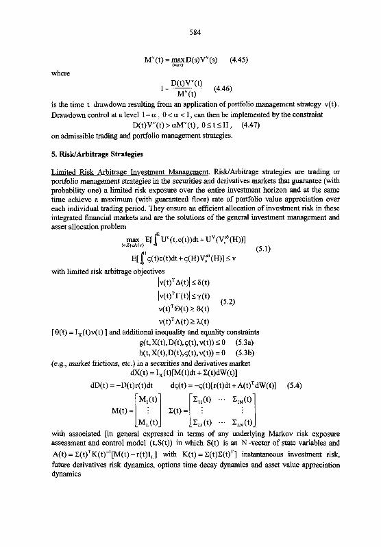
where

is the time t drawdown resulting from an application of portfolio management strategy v(t) . Drawdown control at a level 1 - a , 0 i a < 1, can then be implemented by the constraint

D(t)Vv(t) > aMv(t) , 0 5 t l H , (4.47) on admissible trading and portfolio management strategies.

5. RisWArbitrage Strategies

Limited Risk Arbitrage Investment Management. RisWArbitrage strategies are trading or portfolio management strategies in the securities and derivatives markets that guarantee (with probability one) a limited risk exposure over the entire investment horizon and at the same time achieve a maximum (with guaranteed floor) rate of portfolio value appreciation over each individual trading period. They ensure an efficient allocation of investment risk in these integrated financial markets and are the solutions of the general investment management and asset allocation problem

with limited risk arbitrage objectives

IvWT~(t)l 2 6(t)

v( t ) '~( t ) 2 I(t) [e(t) = I,(t)v(t) ] and additional inequality and equality constraints

g(t,X(t), D(t),~(t),v(t)) 0 (5.34 h(t,X(t),D(t),~(t),v(t)) = 0 (5.3b)

(e.g., market fictions, etc.) in a securities and derivatives market dX(t) = I,(t)[M(t)dt + C(t)dW(t)]

dD(t) = -D(t)r(t)dt dq(t) = -<(t)[r(t)dt +A(t)TdW(t)] (5.4)

M(t) =

with associated [in general expressed in terms of any underlying Markov risk exposure assessment and control model (t,S(t)) in which S(t) is an N -vector of state variables and

A(t) = ~ ( t ) ~ I C ( t ) - l [ ~ ( t ) -r(t)l,] with K(t) = ~ ( t ) ~ ( t ) ~ ] instantaneous investment risk, future derivatives risk dynamics, options time decay dynamics and asset value appreciation dynamics

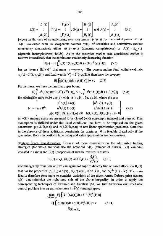
[where in the case of an under ing securities market

and A(t) = [:;I (5.5)

t,S(t)) for the market prices of risk

A(t) associated with the exogenous sources W(t) of securities and derivatives market uncertainty alternatively either A(t) = a(t) (dynamic completeness) or A(t) = GSrv (t)

(dynamic incompleteness) holds]. As in the securities market case considered earlier it follows immediately that the continuous and strictly decreasing function

H(Y) = f S ( ~ ) I ~ ( ~ Y S + S V Y 1 (5.6)

has an inverse [H(Y)]-' that maps v?_T-) yv. The corresponding fund withdrawal rate

c,(t) = IC(t, y,q(t)) and final wealth V,' = I ~ ( ~ ~ S ( H ) ) then have the property

E[E(t)c.(t)dt +s(H)v,'] = v . (5.7)

Furthermore, we have the familiar upper bound

E[ f Uc(t,c(t))dt + uv(v:(~))] I E[f~ ' ( t , c~( t ) )d t + Uv(V,')] (5.8)

for admissible pairs (c,0) EA(v) with v(t) EN,, 0 I t I H ,where the sets

1 InT~(t)l I ~ ( t ) InTr(t)l ~ ( t )

N, = n E R ~ : nT@(t) 2 9(t) n T ~ ( t ) 2 h(t) I (5.9) g(t, Wt), D(t),~(t), n) 5 0 h(t, X(9, D(t),~(t), n) = 0

in v(t) - strategy space are assumed to be closed (with non-empty interior) and convex. This assumption is fulfilled under the usual conditions that have to be imposed on the given constraints g(t,X,D, z,n) and h(t, X, D, z, n) in non-linear optimization problems. Note that in the absence of these additional constraints the origin n = 0 is feasible if and only if the guaranteed floors on portfolio time decay and value appreciation are non-positive.

Stratew S ~ a c e Transformation. Because of these constraints on the admissible trading strategies [for which we shall use the notations v(t) (number of assets), B(t) (amount

invested in assets) and 8(t) (proportion of wealth invested in assets),

interchangeably from now on] we can again not hope to directly find an asset allocation 0,(t)

that has the properties (c,,0,) EA(v), v,(t) EN, , 0 I t I H , and V,'.ev(H) = V,' . The main idea is therefore once more to consider variations of the given Arrow-Debreu price system ~ ( t ) that minimize the right-hand side of the above inequality. In order to apply the corresponding techniques of Cvitanic and Karatzas [63] we fust transform our stochastic control problem into an equivalent one in 8(t) - strategy space

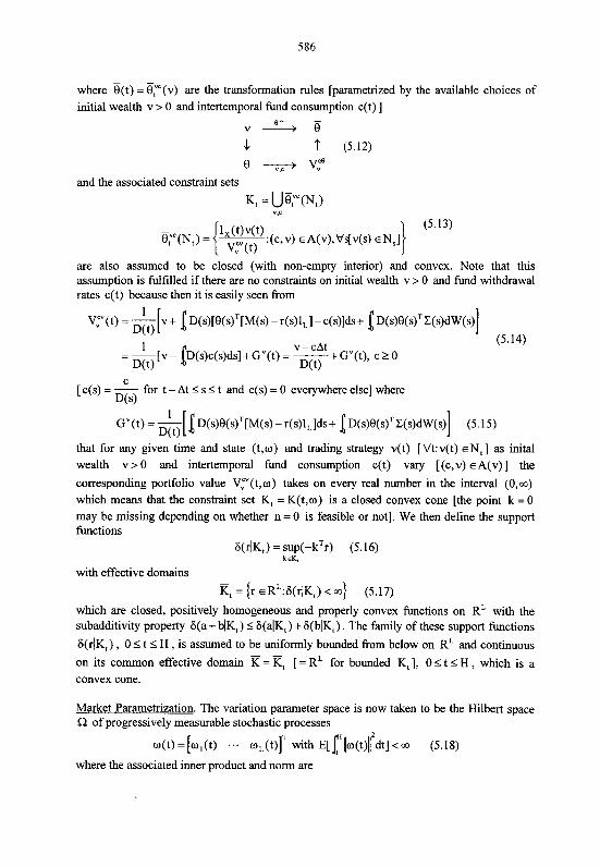
where g(t) = F ( v ) are the transformation rules [parametrized by the available choices of initial wealth v > 0 and intertemporal fund consumption c(t) ]

v"" G J '? (5.12)

@ -G+ Ye and the associated constraint sets

Kt = U ~ ? ( N , ) V,C

are also assumed to be closed (with non-empty interior) and convex. Note that this assumption is fulfilled if there are no constraints on initial wealth v > 0 and fund withdrawal rates c(t) because then it is easily seen from

[ C(S) = for t - At I s t and c(s) = 0 everywhere else] where D(s)

that for any given time and state (t ,o) and trading strategy v(t) [ Vt:v(t) EN, 1 as inital wealth v > 0 and intertemporal fund consumption c(t) vary [(c,v) EA(v)] the

corresponding portfolio value Vy(t,o) takes on every real number in the interval (0,m) which means that the constraint set Kt = K(t,w) is a closed convex cone [the point k = 0 may be missing depending on whether n = 0 is feasible or not]. We then define the support functions

6(rlK,) = sup(-kTr) (5.16) ksK,

with effective domains - K, = {r e ~ ~ : G ( r l K , ) < a } (5.17)

which are closed, positively homogeneous and properly convex functions on R~ with the subadditivity property &(a+ blK,) I S ( a l ~ , ) +S(blK,). The family of these support functions

S ( r l ~ , ) , 0 2 t 2 H , is assumed to be uniformly bounded from below on RL and continuous

on its common effective domain K = K, [= RL for bounded Kt], 0 5 t 5 H , which is a convex cone.

Market Parametrization. The variation parameter space is now taken to be the Hilbert space Q of progressively measurable stochastic processes

w(t) = [w,(t) wL(t)IT with ~[%llw(t)l(dt] < m (5.18)

where the associated inner product and norm are

(w,,w,)= ~ [ ~ w , ( t ) ~ m ~ ( t ) d t ] and 1lw/1= J(W.W). (5.19)

The combined stochastic processes G(w(t)lK,), w E R , are assumed to also be progressively

measurable whenever w(t) ~ f t , 0 I t < H , holds. Moreover, all constant stochastic processes w(t) = w with this property are assumed to belong to the set

For a variation parameter o E fi we next consider the financial market with interest rates

r, (t) = r(t) +G(o(t)lK,) (5.21)

and securities and derivatives price processes

dXp (t) = dx , (t) + X, (t)[w,(t) + G(o(t)lK,)]dt . (5.22)

If c(t) is a fund withdrawal rate and g(t) a trading strategy, then with these asset price dynamics and money market rates the associated portfolio value process is

dV, = [V,GT[M -rl, + o ] + ~ , [ r +G(wlK)]-c]dt + v , G T ~ d w (5.23)

= [V,r -c]dt + ~ , [ 6 ~ o +G(olK)]dt + v,gT&@ [where the factorization with respect to the portfolio value in the second drift term of the above sum is crucial in the following considerations and the reason for choosing g(t) - strategy space]. Note also that with our different notations for trading and portfolio management strategies [i.e., v(t) , 0(t) and g(t) ] we have the equivalent representations

dV = vTdx + [V - vTx]rdt - cdt

= [vT[l,M - rX] + Vr - c]dt + vT1,Cdw

= [oTIM - rl,] + ~r -c]dt +BTZdw (5.24)

= [VgT[M - TI,] + Vr - c]dt + VGTCdw

= [Vr - c]dt + vgTCdB of the associated portfolio value process in the originally given securities and derivatives market. Let for an initial wealth v > 0 now A, (v) be the set of all pairs (c,8) consisting of

a fund withdrawal rate c(t) and a trading strategy g(t) which are admissible in the financial

market parametrized by w(t) and A(v) be the set of all feasible pairs, i.e., originally

admissible pairs (c,G) EA(v) that have the property 8(t) € K t , 0 2 t 2 H . Then we have

A(v) c A, (v) (5.25)

and for every feasible pair (c,8) E A(v),

Vf(t) t V:'(t) , (5.26)

because of the fact that G(t)Io(t) +G(w(t)lK,) 2 0.

Unconstrained Solutions. Furthermore, the general investment management and asset allocation problem

max E[ f uc(t,c(t))dt + U' (v::(H))] (c.%&(v) (5.27)

in the o( t ) -parametrized securities and derivatives market

where c:(t) = I=(~ ,H: - ' (v )~ (t))

V; = I~(H:-I(V)~: (H)) H: (Y) = EI~S:(~)~C(~,~F:(~))~~+~:(H)I~(~S:(H))I (5.30)

[and in the incomplete case the associated Arrow-Debreu price system q: (t) and minimax

local martingale measure f: are again uniquely determined by the investor's utility functions

Uc(t,c) and u V ( v ) ] . If for this optimal o(t)- asset allocation B,"(t) (which is unconstrained) furthermore

@(t) E Kt and B,"(t)Im(t) +6(w(t)lKt) = 0 (5.31)

holds, then the feasible pair (c: ,B,") E A(v) is a solution of the constrained stochastic control problem in the originally given securities and derivatives market and in familiar control theory notation

and

satisfies - ~(v,~:,~,")=~,(v,c:,8,")=~~~,(~.~:,8,m)=V(~)=v,(~)=minv,(~) Sd2 (5.34)

whereas in general only J ( V , C , ~ ) 5 ;$J,(v,c,~), (c,% EA(v), and V(V) 5 ~IIJV,(V) (5.35)

holds.

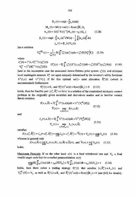
Maximum Principle. If on the other hand c(t) is a fund withdrawal rate and V, a final wealth target such that for a market parametrization o( t )

y p l g,(t)c(t)dt+s.(WvHl= E[ g . ( t M t ) d t + * . ( ~ ) v ~ l = v (5.36)

holds, then there exists a trading strategy q ( t ) that satisfies (c,B,") EA,(v) and

v:: (H) = VH as well as F ( t ) E Kt and B,"(t)T~(t) +6(o(t)lKt) = 0 (see [63] for details).

Therefore the corresponding asset allocation is feasible, i.e., (c,8,") E A(v), and sufficient in

the originally given securities and derivatives market, i.e., v , " ~ (H) = VH . It is optimal if

~ ( t ) = 1~( t ,~ ; (~)5 , ( t ) ) and vH = I~(H;(v)~,(H)) (5.37) holds for some variation parameter C(t) because then

~(v,c,B,") = V,(v). (5.38)

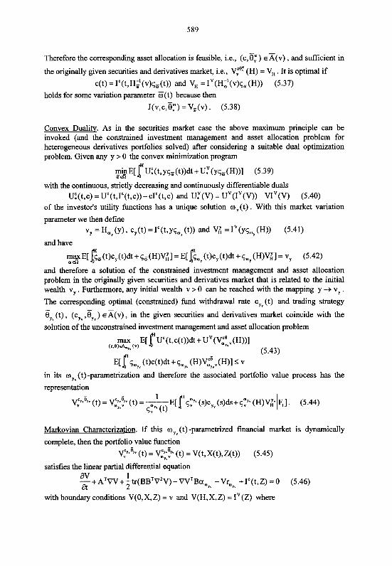
Convex Duality. As in the securities market case the above maximum principle can be invoked (and the constrained investment management and asset allocation problem for heterogeneous derivatives portfolios solved) after considering a suitable dual optimization problem. Given any y > 0 the convex minimization program

with the continuous, strictly decreasing and continuously differentiable duals Uf(t,c) = Uc(t,Ic(t,c))-cIc(t,c) and U:(V) = u ~ ( I ~ ( v ) ) - v I ~ ( v ) (5.40)

of the investor's utility functions has a unique solution oy( t ) . With this market variation

parameter we then define

vy = Hml (Y), cy(t) = I"(~,YS,~ (t)) and Vi = IV(y5,, (H)) (5.41)

and have

d;,(t)cy ( t )d t+s i (wvi l= ~ [ d ; , , ( t ) c y ( W +5- ( H ) ~ i l = vy (5.42)

and therefore a solution of the constrained investment management and asset allocation problem in the originally given securities and derivatives market that is related to the initial wealth v, . Furthermore, any initial wealth v > 0 can be reached with the mapping y -+ v, . The corresponding optimal (constrained) fund withdrawal rate cyv (t) and trading strategy - 8,- (t) , (c," ,8,J EA(v), in the given securities and derivatives market coincide with the

solution of the unconstrained investment management and asset allocation problem

in its o (t) -parametrization and therefore the associated portfolio value process has the

representation 1

(t) = ;-- E[ r 5:" (s)cyv (s)ds+ q:yv ( H ) v ~ ] . (5.44) G,'" (t)

Markovian Characterization. If this a," (t)-parametrized financial market is dynamically

complete, then the portfolio value function

v y ~ " (t) = v$" (t) = V(t,X(t),Z(t)) (5.45)

satisfies the linear partial differential equation av 1 -+A'W +-tr(BBTVZV)- W T B a m Y v - Vr, +Ic(t,Z) = 0 (5.46) at 2

with boundary conditions V(0, X, Z) = v and V(H, X, Z) = I (Z) where

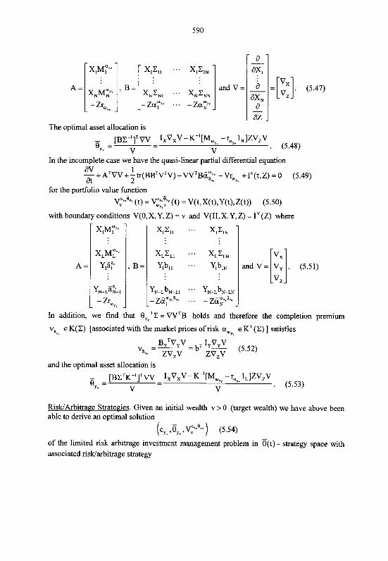
The optimal asset allocation is

(5.48)

In the incomplete case we have the quasi-linear partial differential equation av 1 - + A ~ W + - ~ ~ ( B B ~ V ~ V ) - V V ~ B & ~ ' ~ -Vr, +Ic(t,Z) = 0 (5.49) at 2

for the portfolio value function

~ 2 % " (t) = v,':::" (t) = V(t,X(t),Y(t),Z(t)) (5.50)

with boundary conditions V(O,X,Y,Z) = v and V(H,X,Y,Z) = IV(z) where

and V =

In addition, we find that BYvTC = VV'B holds and therefore the completion premium

v, E K(C) [associated with the market prices of risk aaYv E KL(C) ] satisfies

RisWArbitra~e Strategies. Given an initial wealth v > 0 (target wealth) we have above been able to derive an optimal solution

c , y " , v " ) (5.54)

of the limited risk arbitrage investment management problem in B(t) - strategy space with associated riswarbitrage strategy

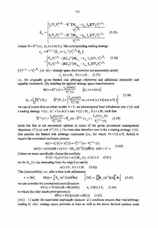
I x x v v v~~~~~ -K-'[M, -ray" I, ]ZV,V,~' .~Y~

,25" - (5.55)

I,v,v>"~ - K - ~ [ M , ~ ~ -ray" ~ J Z V , V ~ ~ ~ ~

p 5 ,

[where 6 = g" (v) , (c, v) E A(v) 1. The corresponding trading strategy = gvcyv-'(e,v) = 1 ~ - y ~ 2 5 ~ e , ~ 1

v ~ "

[V,"'"yv = v," '~~~ ] in v(t) - strategy space does however not necessarily satisfy v , " ( t ) ~ N , , O I t S H , (5.57)

i.e., the originally given limited risk arbitrage objectives and additional inequality and equality constraints. [By recalling the applied strategy space transformation

- - 9(t) = y ( v ) = I (t)v(t) [(c,v) E ~ ( v ) ]

V:'(t)

- (5.58)

K, = ~ B ; " ( N , ) B,"(N,) = lx(t)v(t) .(c,v) ~A(v),V$v(s) EN,] ",F

we can of course find an initial wealth v'> 0 , an intertemporal fund withdrawal rate cl(t) and a trading strategy v'(t) , (c', v') EA(v') and vl(t) EN, , 0 I t I H , such that

holds but this is not necessarily optimal in terms of the given investment management objectives U"(t,c) and u"(v) .] The main idea therefore now is for a trading strategy v'(t) that satisfies the limited risk arbitrage constraints [i.e., for which Vt:vt(t) EN^ holds] to require the associated stochastic process

x(t) = x::(t) = x:.'(t) = v y ' ( t ) - V y " (t) (5.60)

dx(t) = x(t)r(t)dt + (a ' (t) - 1)9yv (t)'~(t)dB(t), x(0) = v'-v

[where we more specifically choose the portfolio 9'(t) = I,(t)vl(t) = a'(t)BYv(t), a ' ( t ) 2 0 (5.61)

on the 9," (t) -ray emanating from the origin] to satisfy

x(t) 2 0 , 0 I t I H . (5.62) This [admissibility, i.e., after a time scale adjustment

t -+ (M), M(t) = [g, ( ~ ) ~ W d $ s ) [(M), = [I19, ( s ) ~ W l r d s ] (5.63)

we can consider the constrained asset allocation dV(t) = V(t)r(t)dt +9(t)dT(t) a, S B(t) 2 b, (5.64)

in which the risky asset's price process is dP(t) = P(t)[r(t)dt +dT(t)] (5.65)

[o(t) = 1 ] under the equivalent martingale measure Q? ] condition ensures that risklarbitrage trading in v(t) - strategy space performs at least as well as the above derived optimal asset

allocation in B(t) - strategy space [in terms of the given investment management objectives

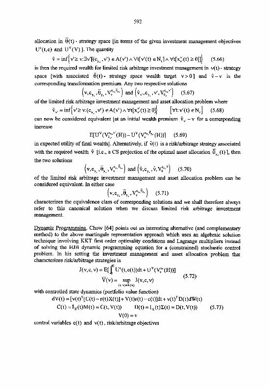
Uc(t,c) and u"(v) 1. The quantity

i = inf(vl> v:3vq[(cyv ,v1) sA(v t ) A Vt[vt(t) E N J A ~t[x:(t) > o]]] (5.66)

is then the required wealth for limited risk arbitrage investment management in v(t) - strategy

space [with associated B(t) - strategy space wealth target v > 0 ] and i - v is the corresponding transformation premium. Any two respective solutions

[v,cyv,~yv,~~'yv)and(iv.,c,,v~,~~~~v~) (5.67)

of the limited risk arbitrage investment management and asset allocation problem where

i,, = inf vq> v:(cyv ,vt ) EA(V') A b't[x:(t) L 011 [vt:vl(t) EN^] (5.68)

can now be considered equivalent [at an initial wealth premium i,. - v for a corresponding

increase

E[U' (V;;:"(H)) - U' (v,'"~" (H))] (5.69)

in expected utility of final wealth]. Alternatively, if G(t) is a risklarbitrage strategy associated

with the required wealth O [i.e., a CS projection of the optimal asset allocation 8," (t) 1, then

the two solutions

(v,cy~,~,v,~~"y)and(i,cyv,&~~i) (5.70)

of the limited risk arbitrage investment management and asset allocation problem can be considered equivalent. In either case

[ v c y y v ) (5.71)

characterizes the equivalence class of corresponding solutions and we shall therefore always refer to this canonical solution when we discuss limited risk arbitrage investment management.

Dynamic Proaamminq. Chow [64] points out an interesting alternative (and complementary method) to the above martingale representation approach which uses an algebraic solution technique involving KKT first order optimality conditions and Lagrange multipliers instead of solving the HJB dynamic programming equation for a (constrained) stochastic control problem. In his setting the investment management and asset allocation problem that characterizes risklarbitrage strategies is

J(v,c,v) = ~ [ f uC(t,c(t))dt +u'(v~(H))] - (5.72) V(v)= sup J(v,c,v)

( C . V ) ~ ( " )

with controlled state dynamics (portfolio value function) dV(t) = [ ~ ( t ) ~ [ c ( t ) - r(t)X(t)] + V(t)r(t) - c(t)]dt + ~ ( t ) ~ ~ ( t ) d ~ ( t )

C(t) = I,(t)M(t) = C(t,V(t)) D(t) = I,(t)Z(t) = D(t,V(t)) (5.73)

V(0) = v control variables c(t) and v(t) , risklarbitrage objectives

~ ( t ) ~ ~ ( t ) 2 h(t) and additional inequality and equality constraints

g(t,V(t),c(t),v(t)) < 0 (5.75)

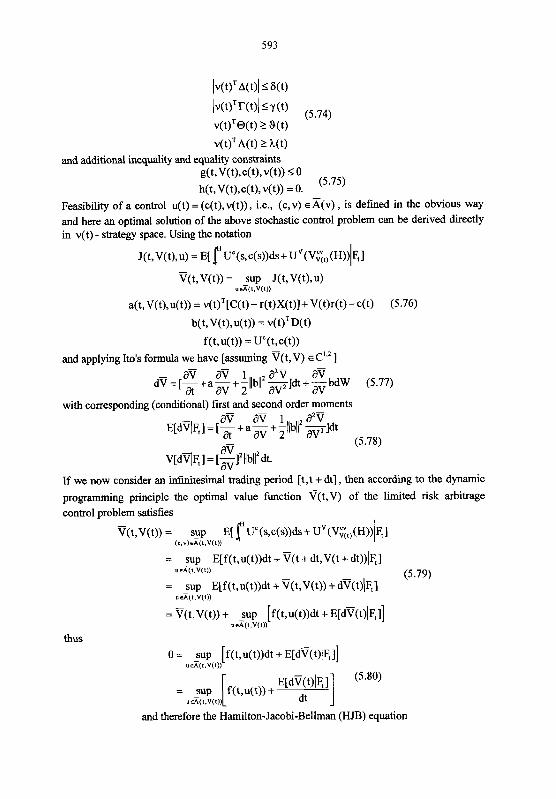
h(t, V(t),c(t), v(t)) = 0. Feasibility of a control u(t) = (c(t), v(t)) , i.e., (c, v) E A(v) , is defined in the obvious way and here an optimal solution of the above stochastic control problem can be derived directly in v(t) - strategy space. Using the notation

and applying Ito's formula we have [assuming V(t, V) E ClS2 ]

a'ir a'ir 1 a2V aV d'ir = [-+a-+-llb112 --~-]dt +-bdW (5.77) a av 2 av av

with corresponding (conditional) first and second order moments aV aV 1 a2V

E[dqF,] = [-+a - + -\lb))2 --~-]dt * (5.78) aV

v[dVl~,] = [-1211blrdt. av If we now consider an infmitesimal trading period [t, t + dt] , then according to the dynamic

programming principle the optimal value function V(t,v) of the limited risk arbitrage control problem satisfies

thus 0 = sup [f(t,u(t))dt + ~[dV(t) l~,]]

"S(I.V(~))

and therefore the Hamilton-Jacobi-Bellman (HJB) equation

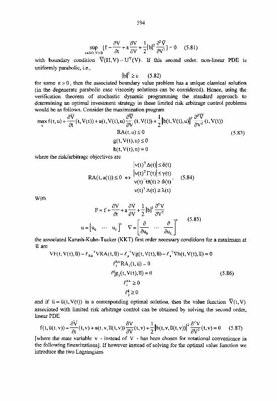
- av aV 1 a2V sup [f+-+a-+-Ilbllz-1-0 (5.81)

u e A ( t , ~ ( t ) ) aV 2 aV2 - with boundary condition V(H,V) = u"(v). If this second order, non-linear PDE is uniformly parabolic, i.e.,

Ilblr 2 E (5.82) for some E > 0 , then the associated boundary value problem has a unique classical solution (in the degenerate parabolic case viscosity solutions can be considered). Hence, using the verification theorem of stochastic dynamic programming the standard approach to determining an optimal investment strategy in these limited risk arbitrage control problems would be as follows. Consider the maximization program

aV aV 1 a2V m y f(t, u) + ~ ( t , ~ ( t ) ) + a ( t , ~ ( t ) , u ) -(t, av ~ t ) ) + -llb(t,~(t),u)ll 2 z ( t , ~ ( t ) )

M ( t , u) 5 0 (5.83)

g(t,V(t),u) 2 0 h(t,V(t),u) = 0

where the risklarbitrage objectives are

Iv(t)'~(t)l5 6(t)

RA(t,u(t)) 2 0 t, /v(t)Tr(t)/ Y (1) (5.84) v(t)T@(t) 2 S(t)

v( t ) '~( t ) 2 h(t)

With

the associated Karush-Kuhn-Tucker (KKT) first order necessary conditions for a maximum at - u are

v~( t ,v ( t ) , i i ) - e M T v u ( t , i i ) - egTVg(t,v(t),ii) -e,Tvh(t,v(t),u) = o e p " ~ ~ , ( t , u ) = 0

eq 2 0

and if ii = E(t,V(t)) is a corresponding optimal solution, then the value function V(t,V) associated with limited risk arbitrage control can be obtained by solving the second order, linear PDE

[where the state variable v - instead of V - has been chosen for notational convenience in the following linearizations]. If however instead of solving for the optimal value function we introduce the two Lagrangians

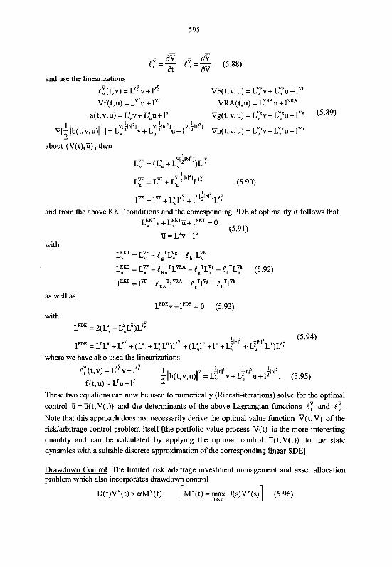
and use the linearizations

e:(t,v) = L'$V+VY VF(~,V,U) = L ~ V + L ~ U + lW

Vf(t,u) = LVfu+lvf VRA(t,u) = LVRAu+1-

a ( t , v , u ) = ~ ~ , v + ~ u + ~ ~ ~ g ( t , v , u ) = L ~ V + L ? u + P (5.89) 1 V+!bl1l v[f#bl21 ~[flbl l ' l

~ [~ / lb ( t ,v .u ) l r ] = Lv v + L, u+ 1 Vh(t,v,u) = L ~ v + L ~ u + ~ "

about (V(t), ti), then

LY = (C" + L,

and from the above KKT conditions and the corresponding PDE at optimality it follows that

These two equations can now be used to numerically (Riccati-iterations) solve for the optimal control ii = ii(t,V(t)) and the determinants of the above Lagrangian functions ey and e!. Note that this approach does not necessarily derive the optimal value function V(t, V) of the riswarbitrage control problem itself [the portfolio value process V(t) is the more interesting quantity and can be calculated by applying the optimal control ti(t,V(t)) to the state dynamics with a suitable discrete approximation of the corresponding linear SDE].

Drawdown Control. The limited risk arbitrage investment management and asset allocation problem which also incorporates drawdown control

D(t)Vv(t) > a t ) [ ~ ' ( t ) = r n a x ~ ( s ) ~ ~ ( $ ] 05sSt (5.96)

at a level 1 - a , 0 < a < 1, can be solved by applying a simple strategy space transformation. Following Cvitanic and Karatzas [65] given such a control level 1 -a we consider the set A: (v) of feasible pairs (c,e') such that the constrained stochastic functional equation

a ~ ' a M ' dv' = [(v' --)O*~[M - rl,] + V'r -c]dt +(v' --)B*~UW

D D (5.97) DV' > aM' ~ ' ( 0 ) = v

has a unique strong (non-negative) solution. Note that for any fund withdrawal rate c(t) and

any RN -valued progressively measurable stochastic process p(t) with

e'(t) = K(t)-'C(t)p(t) (5.98) the above SFE has a unique strong solution

with the property

M?(t) = III~D(s)v:"'(s) = -[~(s)c(s)ds+vex~[(l -a)$(f)] (5.100)

[and that the optimal trading strategies for limited risk arbitrage investment management without drawdown control satisfy OYv(t) =K( t ) - '~ ( t )B( t )~W(t ) ] . Furthermore, if we

compare the stochastic functional equation related to drawdown control with the evolution equation

dV = [0T[M-rl ,]+Vr-c]dt+8TUW, V(0) = v , (5.101) for the portfolio value process used so far, then with a fund withdrawal rate c(t) and a trading

strategy ~ ' ( t ) such that ( c , ~ ' ) EA:(v) by applying the transformation

a~ 0(t) = (v,?' (t) - -

D(t) (t))t3'(t) (5.102)

we find

V,?(t) = V:"'(t). (5.103)

Since the risWarbitrage constraint sets Kt in 6(t) - strategy space are convex cones it is also

clear that (c,e) EA(v). If we therefore (using our equivalent notations for trading strategies) consider the convex cones

R, = P;'(K,) Pt(p) = K(t)-' C(t)p(t) (5.104)

[Kt = {... %(t) ...} with &,(t) = g;(v) 1, then for a progressively measurable process

[ v,? (t) t 0 , 0 I t I H 1. We can thus now define the set (v) A(v) of feasible pairs

(c, 8) for which (c, c) EX: (v) holds with the DC transform

of trading strategy O(t) [given initial wealth v > 0 and fund withdrawal rate c(t) ] and solve the limited risk arbitrage investment management and asset allocation problem with these admissible controls. If (c;" ,Byv ) EX (v) is a corresponding optimal solution, then the

associated portfolio value process satisfies the drawdown constraint at level 1 -a . Note that the relevant constraint sets in 8(t) - strategy space are

KP = TP (Kt) aM:%(t) - T: (R) = (v:" (t) - ------

=Pa oPlt(R,) D(t) )o:,(t) (5.109)

which can be seen to be closed (with non-empty interior) and convex subsets of the riskkirbitrage constraint cones Kt . This is the case because for fixed O'(t) such that

~ t : v ' ( t ) EN, holds as initial wealth v > 0 and intertemporal fund consumption c(t) vary

[ ( c , ~ ' ) E ~ : ( v ) ] the term

MY' (t) D(s)v:&' (s) = max (5.110)

D(~)v?' (t) 'J~'~"(t)v:,e' (t) 1

takes on every value in the interval [I,-). Consequently, the norms Ilgv,(t)ll of the a

corresponding trading strategies - aM'"e' O ( t ) = ( 1 0 ) (5.11 1)

D(~)V?. (t)

[Vy ' ( t ) = ~ > ' ~ ~ ( t ) and Mid'(t) = M;%(t)] take on every value in the interval

(0,(l-a)ll0*(t)ll]. Since the set I,(t)(Nt) of these trading strategies O'(t) is closed (with

non-empty interior) and convex the above conclusion follows.

Partial Observation. In a scenario where the information available to investors in the securities and derivatives market (i.e., the observed asset prices) only partially reflects the history of this market (Karatzas and Xue [66]) we consider a probability space (R, @, x ) with

two (augmented) filtrations { F , ) ~ ~ ~ and {G~),,, that satisfy the usual conditions. The

exogenous sources W(t) of market uncertainty are adapted to the filtration {G,) which therefore records the market history and the coefficients r(t), M(t) and C(t) of the securities and derivatives market model are assumed to be progressively measurable with

respect to {G,} . The filtration {F,} is generated by the asset prices X(t) and thus (in a

Markovian setting) records the market information available to investors. Fund withdrawal rates c(t) and trading strategies O(t) are assumed to be progressively measurable with

respect to {F,} which means that the associated portfolio value processes ~ : ~ ( t ) are also

{F,} -adapted. This follows from the fact that with ~ ( t ) = E[M(~)/F,] and a square root . .

i ( t ,X) of the asset price covariance matrix K(t,X) = C ( t , X ) ~ ( t , x ) ~ the {F,} -adapted

stochastic processes

2, (t) = X,(t) - X,(O) - [X,(s)~,(s)ds (5.1 12)

are continuous, square-integrable {F, ] -martingales that can be represented in the form

with an {F, } - Brownian motion ~ ( t ) . The asset price processes are then

and the value process of an investor's securities and derivatives portfolio evolves according to the linear stochastic differential equation

dV(t) = [ ~ ( t ) ~ [ ~ ( t ) - r(t)l,] + V(t)r(t) -c(t)]dt + ~ ( t ) ~ i ( t , x ( t ) ) d ~ ( t ) . (5.1 15) After this reduction of the partial observations setting to a market model with complete

observations [i.e., all relevant stochastic processes are adapted to the filtration {F,} representing the market information available to investors] we can apply a Girsanov transformation of probability measure

A(t) = i ( t , x ( t ) ) - l [ ~ ( t ) - r(t)l,]

and then solve the limited risk arbitrage investment management and asset allocation problem (with drawdown control) in a dynamically complete financial market.

Final Remark

With our papers RisIdArbitrage Strategies: A New Concept for Asset/Liability Management, Optimal Fund Design and Optimal Porrfolio Selection in a Dynamic, Continuous-Time Framework Part I: Securities Markets and Part 11: Securities and Derivatives Markets we have outlined a very general and powerhl, yet still implementable asset/liability management (ALM) model which focusses on the asset (corporate and investment banking) side. In the paper Baseline for Exchange Rate - Risks of an International Reinsurer, AFIR 1996, Vol. I, p. 395, the liability (reinsurance) side was given equal attention. However, to do so, a significant model extension (optimal control of Markov jump diffusion processes) was necessary. We plan to present such a more sophisticated ALM framework in two forthcomming AFIR publications along the following lines:

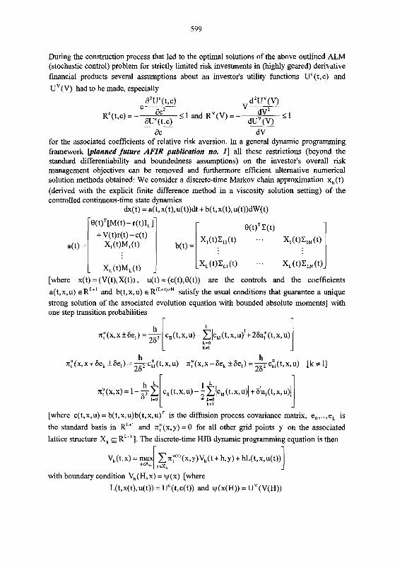
During the construction process that led to the optimal solutions of the above outlined ALM (stochastic control) problem for strictly limited risk investments in (highly geared) derivative financial products several assumptions about an investor's utility functions Uc(t,c) and

u V ( v ) had to be made, especially

d2~ ' ( t t , c ) c-

dZuV(V)

R'(~,c)=- aC2 5 1 and R ~ ( v ) = - v~ auc(t,c) d u V ( v ) 'I & dV

for the associated coefficients of relative risk aversion. In a general dynamic programming framework [planned future AFZR publication no. I ] all these restrictions (beyond the standard differentiability and boundedness assumptions) on the investor's overall risk management objectives can be removed and furthermore efficient alternative numerical solution methods obtained: We consider a discrete-time Markov chain approximation xh(t) (derived with the explicit finite difference method in a viscosity solution setting) of the controlled continuous-time state dynamics

[where x(t) = (V(t),X(t)) , u(t) = (c(t),e(t)) are the controls and the coefficients

a(t,x,u) €RL+' and b(t,x,u) E R ' ~ " ) " ~ satisfy the usual conditions that guarantee a unique strong solution of the associated evolution equation with bounded absolute moments] with one step transition probabilities

r 1

[where c(t, x, u) = b(t, x, u) b(t, x, u ) ~ is the diffusion process covariance matrix, e, ,. . , e, is

the standard basis in RL" and x:(x,y) = 0 for all other grid points y on the associated

lattice structure X, E RLt' 1. The discrete-time HJB dynamic programming equation is then

I

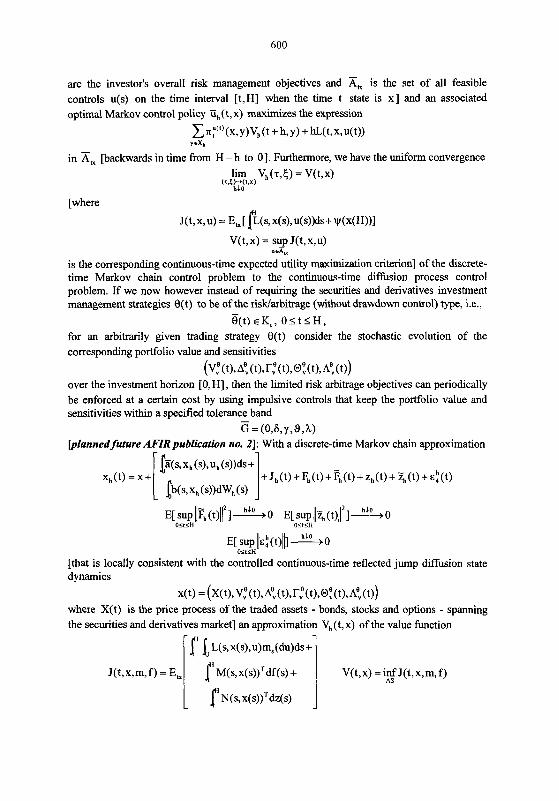
are the investor's overall risk management objectives and A, is the set of all feasible controls u(s) on the time interval [t,H] when the time t state is x] and an associated optimal Markov control policy Tih(t,x) maximizes the expression

Z ~ : " ' ( X , Y ) V ~ ( ~ + h,y) +h~(t,x,u(t)) YE%

in A, [backwards in time fiom H - h to 01. Furthermore, we have the uniform convergence

V(t,x) = sup J(t,x,u) u G . .

is the corresponding continuous-time expected utility maximization criterion] of the discrete- time Markov chain control problem to the continuous-time diffusion process control problem. If we now however instead of requiring the securities and derivatives investment management strategies 8(t) to be of the riswarbitrage (without drawdown control) type, i.e.,

for an arbitrarily given trading strategy O(t) consider the stochastic evolution of the

over the investment horizon [O,H], then the limited risk arbitrage objectives can periodically be enforced at a certain cost by using impulsive controls that keep the portfolio value and sensitivities within a specified tolerance band

G = ( 0 , 6 , ~ , 9 , ~ [planned future AFZRpublication no. 21: With a discrete-time Markov chain approximation

[that is locally consistent with the controlled continuous-time reflected jump diffusion state dynamics

x(t) = (~(t),~,e(t),~:(tt,r,e(t),@:(t),~:(t)) where X(t) is the price process of the traded assets - bonds, stocks and options - spanning the securities and derivatives market] an approximation Vh (t, x) of the value function

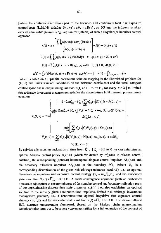
[where the continuous reflection part of the bounded and continuous total risk exposure control costs (L,M,N) satisfies N(t, y)Tr 2 0, r eR(y), on aG and the infimum is taken over all admissible (relaxedfsingular) control systems] of such a singular (or impulse) control approach

Z(s, x(s), u)m,(du)ds + x(t) = x+ I + J(t) + F(t) + z(t)

s,x(s))dW(s)

I

~ ( t ) = C r , < ( t ) ri E R ( ~ , ) , y, EX f,(t)20, df,(t)20 i=l

z(t) = [r(s)d~d(s), r(s) E R(x(s)) [PAW a.e.1 1z-b = [ 4(s,ad~d(s)

[which is based on a Lipschitz continuous solution mapping in the Skorokhod problem for (G,R) and under standard conditions on the diffusion coefficients and the usual compact

control space has a unique strong solution x(t) E G , 0 5 t 5 H , for every x E G ] to limited risk arbitrage investment management satisfies the discrete-time HJB dynamic programming equation

V,(t,x) = min

V, (H, x) = 0.

By solving this equation backwards in time from tkb-, [tkb = HI to 0 we can determine an

optimal Markov control policy ii,(t,x) [which we denote by i$(du) in relaxed control

notation], the corresponding (optimal) intertemporal singular control impulses ATh(t,x) and

the necessary reflection impulses AZ,(t,x) at the boundary aG, (where G, is a

corresponding discretization of the given risklabitrage tolerance band G), i.e., an optimal discrete-time impulsive risk exposure control strategy (ii, = Ei, , ?, ,z,) and the associated

state evolution Tl, (t) E G, , 0 5 t < H . A weak convergence argument [with an embedded time scale adjustment to ensure tightness of the singular control and boundary reflection parts of the approximating discrete-time state dynamics x,(t) ] then also establishes an optimal solution of the initially given continuous-time impulsive limited risk arbitrage investment management problem, i.e., a continuous-time optimal impulsive risk exposure control strategy (m, T,z) and the associated state evolution x(t) E G , 0 < t < H . The above outlined HJB dynamic programming framework (based on the Markov chain approximation technique) also turns out to be a very convenient setting for a full extension of the concept of

limited risk arbitrage investment management to a financial market with discontinuous securities and derivatives price processes. Such a generalization and extension then implements an optimal combination of continuous risWarbitrage control (i.e., expected utility maximization under given risk exposure constraints) and impulsive risk exposure control (i.e., minimization of the exposure control costs associated with a given risky trading or portfolio management strategy).

Appendix: References

[ l ] I. Karatzas, Optimization Problems in the Theory of Continuous Trading, SIAM Journal Control and Optimization 27, 1221 - 1259 (1 989) [2] J. C. Cox and C.-F. Huang, Optimal Consumption and Portfolio Policies when Asset Prices Follow a Diffusion Process, Joumal of Economic Theory 49,33-83 (1989) [3] C.-F. Huang, Information Structure and Equilibrium Asset Prices, Journal of Economic Theory 35,33-71 (1985) [4] D. Duffie, Stochastic Equilibria: Existence, Spanning Number, and the 'No Expected Financial Gain from Trade' Hypothesis, Econometrica 54,1161-1 183 (1 986) [5] D. Duffie and C.-F. Huang, Implementing Arrow-Debreu Equilibria by Continuous Trading of Few Long-Lived Securities, Econometrica 53,1337-1356 (1985) [6] S. Krasa and J. Werner, Equilibria with Options: Existence and Indeterminacy, Journal of Economic Theory 54,305-320 (1991) [7] C.-F. Huang, An Intertemporal General Equilibrium Asset Pricing Model: The Case of Diffusion Information, Econometrica 55, 11 7-142 (1 987) [8] I. Karatzas, J. P. Lehoczky and S. E. Shreve, Existence and Uniqueness of Multi- Agent Equilibrium in a Stochastic, Dynamic Consumption/Investrnent Model, Mathematical Operations Research 15,80-128 (1990) [9] A. Hindy and C.-F. Huang, Intertemporal Preferences for Uncertain Consumption: A Continuous Time Approach, Econometrica 60,781-801 (1992) [lo] H. Foellmer and M. Schweizer, A Microeconomic Approach to Diffusion Models for Stock Prices, Mathematical Finance, Vol. 3, No. 1, 1-23 (1993) [I 11 D. B. Madan and F. Milne, Option Pricing With V. G. Martingale Components, Mathematical Finance, Vol. 1, No. 4, 39-55 (1991) [12] I. Karatzas, J. P. Lehoczky and S. E. Shreve, Equilibrium Models with Singular Asset Prices, Mathematical Finance, Vol. 1, No. 3, 11-29 (1991) [13] P. H. Dybvig and C.-F. Huang, Nonnegative Wealth, Absence of Arbitrage, and Feasible Consumption Plans, Revue of Financial Studies 1, 377-401 (1988) [14] D. C. Heath and R. A. Jarrow, Arbitrage, Continuous Trading, and Margin Requirements, Journal of Finance 42,1129-1 142 (1987) [15] R. A. Jarrow and D. B. Madan, A Characterization of Complete Security Markets on a Brownian Filtration, Mathematical Finance, Vol. 1, No. 3,31-43 (1991) [16] M. Chatelain and C. Stricker, On Componentwise and Vector Stochastic Integration, Mathematical Finance, Vol. 4, No. 1, 57-65 (1994) [I71 C. Stricker, Arbitrage et Lois de Martingale, Annales de I'Institut Henri Poincare 26, 45 1-460 (1990) [18] F. Delbaen, Representing Martingale Measures When Asset Prices Are Continuous and Bounded, Mathematical Finance, Vol. 2, No. 2, 107-130 (1992) [19] P. Lakner, Martingale Measures for a Class of Right-Continuous Processes, Mathematical Finance, Vol. 3, No. 1,43-53 (1993)

[20] K. I. Amin and R. A. Jarrow, Pricing Options on Risky Assets in a Stochastic Interest Rate Economy, Mathematical Finance, Vol. 2, No. 4,217-237 (1992) [21] S. T. Cheng, On the Feasibility of Arbitrage-Based Option Pricing When Stochastic Bond Prices Are Involved, Journal of Economic Theory 53, 185-198 (1991) [22] D. Heath, R. A. Jarrow and A. Morton, Bond Pricing and the Term Structure of Interest Rates: A New Methodology for Contingent Claims Valuation, Econornetrica 60, 77- 105 (1992) [23] R. J. Brenner and J. L. Denny, Arbitrage Values Generally Depend on a Parametric Rate of Return, Mathematical Finance, Vol. 1, No. 3,45-52 (1991) [24] D. Duffle and L. G. Epstein, Stochastic Differential Utility, Econornetrica 60, 353- 394 (1992) [25] J. B. Detemple and F. Zapatero, Optimal Consumption-Portfolio Policies With Habit Formation, Mathematical Finance, Vol. 2, No. 4,251-274 (1992) [26] S. Wang, The Integrability Problem of Asset Prices, Journal of Economic Theory 59, 199-213 (1993) [27] H. He and H. Leland, On Equilibrium Asset Price Processes, Revue of Financial Studies 6,593-617 (1993) [28] H. He and C.-F. Huang, Consumption-Portfolio Policies: An Inverse Optimal Problem, Journal of Economic Theory 62,257-293 (1994) [29] I. Karatzas, J. P. Lehoczky, S. E. Shreve, and G.-L. Xu, Utility Maximization in an Incomplete Market, SIAM Journal Control and Optimization 29,703-730 (1989) [30] H. He and N. D. Pearson, Consumption and Portfolio Policies with Incomplete Markets and Short-Sale Constraints: The Infinite Dimensional Case, Journal of Economic Theory 54,259-304 (1991) [31] S. D. Jacka, A Martingale Representation Result and an Application to Incomplete Financial Markets, Mathematical Finance, Vol. 2, No. 4,239-250 (1992) [32] H. Foellmer and D. Sondermann, Hedging of Non-redundant Contingent Claims, Contributions to Mathematical Economics 1986 [33] M. Schweizer, Risk-Minimality and Orthogonality of Martingales, Stochastics 30, 123-131 (1990) [34] R. J. Elliott and H. Foellmer, Orthogonal Martingale Representation, Stochastic Analysis, Academic Press 1991 [35] H. Foellmer and M. Schweizer, Hedging of Contingent Claims under Incomplete Information, Applied Stochastic Analysis, Gordon and Breach 1991 [36] M. Schweizer, Option Hedging for Semimartingales, Stochastic Processes and their Applications 37,339-363 (1991) [37] M. Schweizer, Martingale Densities for General Asset Prices, Journal of Mathematical Economics 21,363-378 (1992) [38] J. P. Ansel and C. Stricker, Lois de Martingale, Densites et Decomposition de Foellmer Schweizer, Annales de 1'Institut Henri Poincare 28, 375-392 (1992) [39] N. Hofinann, E. Platen and M. Schweizer, Option Pricing Under Incompleteness and Stochastic Volatility, Mathematical Finance, Vol. 2, No. 3, 153-187 (1992) [40] D. B. Colwell and R. J. Elliott, Discontinuous Asset Prices and Non-Attainable Contingent Claims, Mathematical Finance, Vol. 3, No. 3,295-308 (1993) [41] W. Schachermayer, A Counterexample to Several Problems in the Theory of Asset Pricing, Mathematical Finance, Vol. 3, No. 2,217-229 (1993) [42] N. Bouleau and D. Lamberton, Residual Risks and Hedging Strategies in Markovian Markets, Stochastic Processes and their Applications 33, 13 1-150 (1989) [43] S. A. Ross, Options and Efficiency, Quarterly Journal of Economics 90, 75-89 (1976)

[44] F. D. Arditti and K. John, Spanning the State Space with Options, Journal of Financial and Quantitative Analysis 15, 1-9 (1980) [45] K. John, Efficient Funds in a Financial Market with Options: A New Irrelevance Proposition, Journal of Finance 36,685-695 (1981) [46] K. John, Market Resolution and Valuation in Incomplete Markets, Journal of Financial and Quantitative Analysis 19,29-44 (1984) [47] R. C. Green and R. A. Jarrow, Spanning and Completeness in Markets with Contingent Claims, Journal of Economic Theory 41,202-210 (1987) [48] D. C. Nachman, Spanning and Completeness with Options, Revue of Financial Studies 1, 31 1-328 (1988) [49] J.-C. Duan, A. F. Moreau and C. W. Sealey, Spanning With Index Options, Journal of Financial and Quantitative Analysis 27,303-309 (1992) [50] P. Zipkin, The Relationship Between Risk and Maturity in a Stochastic Setting, Mathematical Finance, Vol. 2, No. 1,33-46 (1992) [5 11 J. Cox, J. Ingersoll and S. Ross, Duration and the Measurement of Basis Risk, Journal of Business 52,5 1-61 (1979) [52] J. Cox, J. Ingersoll and S. Ross, A Theory of the Term Structure of Interest Rates, Econometrics 53,385-407 (1985) [53] R. S. Sears and G. L. Trennepohl, Measuring Portfolio Risk in Options, Journal of Financial and Quantitative Analysis 17,391-409 (1982) [54] E. Elton and M. Gruber, Risk Reduction and Portfolio Size: An Analytical Solution, Journal of Business 50,415-437 (1977) [55] J. R. Booth, H. Tehranian and G. L. Trennepohl, Efficiency Analysis and Option Portfolio Selection, Journal of Financial and Quantitative Analysis 20,435-450 (1985) [56] G. A. Whitmore, Third Degree Stochastic Dominance, American Economic Review 60,457-459 (1970) [57] H. Levy and Y. Kroll, Ordering Uncertain Options with Borrowing and Lending, Journal of Finance 33,553-574 (1 978) [58] H. Levy and Y. Kroll, Efficiency Analysis with Borrowing and Lending, Review of Economics and Statistics 61, 125-1 30 (1 979) [59] W. H. Jean, The Geometric Mean and Stochastic Dominance, Journal of Finance 35, 151-158 (1980) [60] D. Lamberton and B. Lapeyre, Hedging Index Options With Few Assets, Mathematical Finance, Vol. 3, No. 1,25-41 (1993) [61] M. Jeanblanc-Picque, Impulse Control Method and Exchange Rate, Mathematical Finance, Vol. 3, No. 2, 161-177 (1993) [62] S. J. Grossman and Z. Zhou, Optimal Investment Strategies for Controlling Drawdowns, Mathematical Finance, Vol. 3, No. 3,241-276 (1993) [63] J. Cvitanic and I. Karatzas, Convex Duality in Constrained Portfolio Optimization, Annals of Applied Probability 2,767-8 18 (1 992) [64] G. C. Chow, Optimal Control Without Solving the Bellman Equation, Journal of Economic Dynamics and Control 17,621-630 (1993) [65] J. Cvitanic and I. Karatzas, On Poruolio Optimization Under Drawdown Constraints, Department of Statistics, Columbia University, New York, 1994 [66] I. Karatzas and X.-X. Xue, A Note on Utility Maximization Under Partial Observation, Mathematical Finance, Vol. 1, No. 2, 57-70 (1991) [67] I. Karatzas and S. E. Shreve, Brownian Motion and Stochastic Calculus, Graduate Texts in Mathematics, Springer 1991

[68] P. Protter, Stochastic Integration and Dlfjerential Equations: A New Approach, Applications of Mathematics, Springer 1990 [69] R. S. Liptser and A. N. Shiryayev, Statistics of Random Processes I: General Theory, Applications of Mathematics, Springer 1977 [70] R. S. Liptser and A. N. Shiryayev, Statistics of Random Processes II: Applications, Applications of Mathematics, Springer 1978 [71] A. N. Shiryayev, Probability, Graduate Texts in Mathematics, Springer 1984 [72] J. Jacod and A. N. Shiryayev, Limit Theorems for Stochaslic Processes, Grundlehren der mathematischen Wissenschaften, Springer 1987 [73] R. J. Elliott, Stochastic Calculus and Applications, Applications of Mathematics, Springer I982 [74] S. N. Ethier and T. G. Kurtz, Markov Processes: Characterization and Convergence, Wiley 1986 [75] W. H. Fleming and H. M. Soner, Controlled Markov Processes and Viscosity Solutions, Applications of Mathematics, Springer 1993 [76] M. S. Bazaraa, H. D. Sherali and C. M. Shetty, Nonlinear Programming: Theory and Algorithms, Wiley 1993 [77] K. Yosida, Functional Analysis, Springer 1980 [78] W. Rudin, Functional Analysis, International Series in Pure and Applied Mathematics, McGraw-Hill 1991