Journal of

Marine Science and Engineering

Article

Optimal Damping Concept Implementation for Marine Vessels’Tracking Control

Evgeny I. Veremey

�����������������

Citation: Veremey, E.I. Optimal

Damping Concept Implementation

for Marine Vessels’ Tracking Control.

J. Mar. Sci. Eng. 2021, 9, 45. https://

doi.org/10.3390/jmse9010045

Received: 26 November 2020

Accepted: 29 December 2020

Published: 4 January 2021

Publisher’s Note: MDPI stays neu-

tral with regard to jurisdictional clai-

ms in published maps and institutio-

nal affiliations.

Copyright: © 2021 by the author. Li-

censee MDPI, Basel, Switzerland.

This article is an open access article

distributed under the terms and con-

ditions of the Creative Commons At-

tribution (CC BY) license (https://

creativecommons.org/licenses/by/

4.0/).

Computer Applications and Systems Department, Saint-Petersburg State University, Universitetskii Prospekt 35,Petergof, 198504 Saint Petersburg, Russia; e_veremey@mail.ru

Abstract: This work presents the results of studies related to the design of stabilizing feedbackconnections for marine vessels moving along initially given trajectories. As is known, in mathematicalformalization, this question leads to a problem of tracking control synthesis for nonlinear and non-autonomous plants. To provide desirable stability and performance features of the closed-loopsystems to be synthesized, it is appropriate to use an optimization approach. Unlike the knownsynthesis methods, which are usually used within the framework of this approach, it is proposed toimplement the optimal damping concept first developed by V.I. Zubov in the early 60s of the lastcentury. Modern interpretation of this concept allows constructing numerically effective proceduresof control law synthesis taking into account its applicability in a real-time regime. Central attentionis focused on the questions connected with practical adaptation of the optimal damping methods formarine control systems. The operability and effectiveness of the proposed approach are illustratedby a practical example of tracking control design.

Keywords: marine vessel; tracking controller; stability; functional; optimal damping

1. Introduction

The nonlinear tracking control of modern marine vessels is one of the most practicallysignificant and theoretically considerable problems in the area of automatic control analysisand design. In particular, tracking control systems are widely used in different branchessuch as hydrography, inspection of marine constructions, wreck investigation, underwatercable laying, and so on [1,2]. Central theoretical and practical background of trackingcontrol for various moving plants is presented in [3–5] and other fundamental works.

Various issues associated with the design of tracking controllers for marine surfacevessels have already been extensively researched and presented in numerous publications(for example, [1,2,6–16]). To evaluate the state of the art in marine tracking control, let usaddress some modern works presenting this direction of research.

Currently, it is possible to use various ideas to design nonlinear tracking control lawsthat are reflected in numerous publications, for example, [7,8,13–16]. However, let us notethat the mentioned works are not directly oriented to the application of the optimizationtechnique. This makes it difficult to provide the desired dynamic features of the closed-loop connections. Now, it seems to be quite evident that the most effective analyticaland numerical tool for feedback connections design is the optimization approach. Severalaspects of nonlinear tracking control optimization technique are presented in multitudinousscientific publications, including such popular monographs as [4,5,17–21]. As for thesimplest stabilization problem, the autopilots with multipurpose structures of optimizedcontrol laws are discussed in detail in [22–26].

The sliding mode control technique for marine control applications is discussedin [1,2,6,8]. This direction seems to be quite constructive, but poorly applicable, since itleads to intensive wear of the actuators.

J. Mar. Sci. Eng. 2021, 9, 45. https://doi.org/10.3390/jmse9010045 https://www.mdpi.com/journal/jmse

J. Mar. Sci. Eng. 2021, 9, 45 2 of 15

As for the model predictive control (MPC) approach [9], its most significant disadvan-tage is the large dimension of the minimization problem that is solved at each step of thecontrol process.

Notably, the complexity of this problem is vast because of the many dynamic require-ments, restrictions, and conditions that must be satisfied by the chosen control actions.

It should be noted that many scientific works devoted to the tracking control formarine vessels use linear time invariant models of their motion. However, such models arenot quite adequate for the problems of deep maneuvering control in angle and positionaldynamic variables. Respectively, one of the most important practical difficulties requiringconsideration in the design process is the account of nonlinearity and non-autonomy of thecontrol plant model. In most cases, this problem is a source of dynamic instability and poorperformance for various systems that were designed based only on linear approximations.

As for the aforementioned optimization approach, its advantages are determinedby the flexibility and convenience of modern optimization methods with respect to therelevant practical demands for control design implementation. Certain analytical andnumerical methods are used now to compute the optimal controllers for nonlinear andnon-autonomous systems subject to various given performance indices. Nevertheless, thereis no saying that the optimization approach is recognized overall as a universal instrumentto be put into practice for marine tracking controllers design. This can be explained by thepresence of some disadvantages connected with computational troubles. Therefore, thereexists a vital necessity to develop persistently analytical and numerical methods of controllaws design based on optimization ideology adapting to the specific problems for variousmarine applications.

At present time, numerous approaches are used for a practical solution of theseproblems [1–12,17,18]. Usually, they are based on Pontryagin’s maximum principle, onBellman’s dynamic programming principle, on finite-dimensional approximation in therange of model predictive control (MPC) technique, etc. Unfortunately, all these approachesare connected with the huge extent of calculations that essentially impedes their implemen-tation both for laboratory design activity and real-time regimes of control.

The existence of numerical difficulties motivates us to use other approaches that allowavoiding the aforementioned shortcomings. This work focuses on a different concept thatcan be applied to design tracking controllers using the theory of optimal damping (OD).This theory, which was first proposed and developed by V.I. Zubov in his works [19–21],provides effective analytical and numerical methods for control calculations with essentiallyreduced computational consumptions with respect to classical techniques. We believe thatthis theory was ahead of its time and was undeservedly underutilized for practical controlproblem solving. This work is one of the attempts to overcome this omission, taking intoaccount the impressive development of modern computer technologies.

In this article, special attention is paid to the control of marine vessels in terms of theforward speed and heading angle. We are considering the regime of the acceleration in or-der to achieve the specified forward speed with one-time turn along the heading. To achievedesirable stability and performance features of the reference motion, the correspondenttracking controllers were designed based on the OD technique.

The main contribution of this paper is determined by the following statements. First,we propose to use the OD concept to design tracking controllers for marine vessel speedand heading. This has not been the case before. Second, we discuss a new methodologyfor selecting the functional to be damped, taking into account the desirable features ofthe closed-loop system in the range of the optimization technique. Hereby, the choice ofthis functional as the basis is argued by the guarantee asymptotic stability and the desiredquality of control processes. Third, we point to the possibility of applying the OD approachto a wide class of nonlinearities in the mathematical model of the vessel. It is noted thatthis approach can be implemented in real-time regime of a ship’s motion. The practicalapplicability and effectiveness of the proposed technique is illustrated by a controllerdesign for a transport marine ship.

J. Mar. Sci. Eng. 2021, 9, 45 3 of 15

The novelty of the proposed approach with respect to other works lies in the univer-sality and flexibility of proposed nonlinear non-autonomous control laws based on ODcomputational procedure, which can be implemented in a real-time regime of functioningfor marine control plants.

In general, the present study is an extension of the multipurpose approach proposedin [22–27] and developed in [28] with respect to the marine autopilot control laws with thenovel structure, taking into account actuators’ time delays.

This article is organized as follows. In Section 2, the optimal damping concept for con-trol law synthesis for nonlinear non-autonomous systems is discussed, taking into accountcertain specific stability and performance requirements for marine control applications.The known background is presented, and the novel ways are proposed to provide tracingcontrollers synthesis. Section 3.1 is devoted to the OD synthesis problem statement for theforward speed tracking controller and for the tracking autopilot. Central attention is paidto the presentation of mathematical models of the control plant and dynamic requirementsfor the quality of the closed-loop connection. Section 3.2 presents an exhaustive novelsolution for the mentioned synthesis problem based on the optimal damping concept. InSection 3.3, a practical example of tracking controller synthesis is presented to illustrate theapplicability and effectiveness of the proposed approach. Finally, Section 4 concludes thearticle by discussing the overall results of the investigation and indicates how these resultscan be further developed.

2. Materials and Methods

As mentioned above, the essence of this paper involves developing an optimal damp-ing technique of tracking control law synthesis for marine vessels with nonlinear andnon-autonomous models. In this section, let us first consider the background and someessential features of the OD approach that define the methodological basis of the study.

First of all, let us introduce a commonly used nonlinear robot-like model of the controlplant, which represents marine vessel motion for various regimes of its operation [1,2,6]:

M.ν+ C(ν)ν+ D(ν)ν+ g(η) = Guτ+ d,

.η = J(η)ν,

(1)

where vector ν ∈ Rn presents velocities defined in a plant-fixed frame and vector η ∈ Rn

contains position dynamical parameters (displacements and angles) in an Earth-fixedframe. External disturbances and controls are presented by the vectors d ∈ Rn and τ ∈ Rm,respectively. Let us accept that the inertia matrix is positive definite: M = MT > 0,the matrix of Coriolis-centripetal terms is skew-symmetrical: C(ν) = −CT(ν), and thedamping matrix D(ν) > 0 is positive definite but non-symmetrical. Vector g(η) representsgravitational and buoyancy forces and moments, J(η) is the matrix of rotations, and thematrix Gu with the constant components reflects controls allocation.

Let us provide a transformation of the body-fixed frame representation (1) to theEarth-fixed one with respect to the vector η. Following [1], this can be done using thefollowing notations:

Mη(η) := J−T(η)MJ−1(η),Cη(ν,η) := J−T(η)

[C(ν)−MJ−1(η)

.J(η)

]J−1(η),

Dη(ν,η) := J−T(η)D(ν)J−1(η), gη(η) := J−T(η)g(η),τη := J−T(η)Guτ, dη = J−T(η)d.

(2)

In accordance with (2), initial model (1) of the plant takes the form:

..η = −M−1

η (η)((Cη(ν,η) + Dη(ν,η))

.η+ gη(η) − τη − dη

), ν = J−1(η)

.η . (3)

J. Mar. Sci. Eng. 2021, 9, 45 4 of 15

The essence of the tracking control problem is to provide given desirable motionη = ηd(t) of the vessel, using the following state feedback

τ = τ(η,ν,ηd(t)), (4)

which is a nonlinear non-autonomous tracking controller.Within mathematical formalization, controller (4) must be implemented to provide the

zero equilibrium with respect to the tracking error e(t) := η(t)− ηd(t) for the closed-loopsystem (3), (4), where d(t) ≡ 0. Naturally, this equilibrium point must be asymptoticallystable to guarantee that e(t)→ 0 as t→ ∞ . Let us especially note that the mentionedclosed-loop system is nonautonomous, if we have no constant reference motion ηd(t).This gives reasons for us to require the uniform asymptotic stability in global (UGAS) orlocal (UAS) form. An additional requirement is that the controller (4) provides the desireddynamical features for the closed-loop system (3), (4) under the action of an admissiblecontrol τ ∈ Tu.

To set the perform of the controller (4) synthesis, we assume that the vector functionsηd(t), ν(t) := J−1(ηd(t))

.ηd(t), and the corresponding τd(t) are given. These functions

satisfy Equations (1) or (3), i.e., we have:

M.νd(t) + C(νd(t))νd(t) + D(νd(t))νd(t) + g(ηd(t)) ≡ Guτd(t),.

ηd(t) ≡ J(ηd(t))νd(t).(5)

Let introduce the following additional notations:

~x :=

(~x1~x2

)=

(ν

η

), f(

~x) :=

(−M−1[C(ν) + D(ν)]ν−M−1g(η)

J(η)ν

), B :=

(M−1Gu

0

)which allows us to present Equations (1) and (5) as

.~x = f(

~x) + Bτ,

.xd ≡ f(xd) + Bτd, (6)

supposing that d(t) ≡ 0.Let us also consider deflections

x :=~x− xd =

(x1x2

):=(

eνe

):=(ν− νdη− ηd

), u := τ− τd (7)

of the vessel dynamical parameters from the desirable motion.Then, we can present equations of the vessel in the deflections from the desirable

motion. Using notations (7) on the base of (6), we obtain

.x = α(t, x) + Bu, (8)

where

α(t, x) = α(t, e, eν) :=(−M−1[C(eν + νd(t)) + D(eν + νd(t))](eν + νd(t))−M−1g(e + ηd(t))

J(e + ηd(t))(eν + νd(t))

)−(

−M−1[C(νd(t)) + D(νd(t))]νd(t)−M−1g(ηd(t))J(ηd(t))νd(t)

).

(9)

It is a matter of simple calculations to check that equation (6) has zero equilibriumposition, which must be stabilized by the choice of the controller u = u(t, x). If thiscontroller is found, then the tracking feedback (4) can be presented as

τ = τ(t,ν,η) = τ(η,ν,ηd) = u(t, x) + τd(t), x :=(ν− νd(t)η− ηd(t)

). (10)

J. Mar. Sci. Eng. 2021, 9, 45 5 of 15

As for the desirable dynamic features of the closed-loop connection, the most widelyused formalized approach is based on minimizing the following integral functional:

J = J(t, x, u) =∞∫

t0

f (τ, x, u) dτ,

that determines the quality of control processes for a closed-loop system. Here, subintegralfunction f is positive definite, i.e., f (t, x, u) ≥ 0 ∀t ≥ t0, ∀x, ∀u, f = 0⇔ x = 0, u = 0.However, as is well known, there are certain difficulties in directly implementing thisapproach, which are determined by the huge extent of calculations that essentially impedestheir practical implementation.

We propose to overcome the mentioned obstacles using a novel technique based onthe OD concept, connected to the OD problem for the synthesis of the control u. To statethis problem, firstly, let us introduce the functional to be damped as follows:

L = L(t, x, u) = V(t, x) +t∫

t0

f0(τ, x, u) dτ, (11)

where V = V(t, x) is a Lyapunov function candidate, and f0 is a positively defined function.Let us additionally accept that the function V satisfies the following conditions:

α1(‖x‖) ≤ V(t, x) ≤ α2(‖x‖)∀x ∈ Br ⊂ En, ∀t ≥ t0, (12)

where α1,α2 ∈ K are comparison functions [4].The essence of the OD approach consists of the control generation as a function from

the current values of variables t, x in the form

u0 = u0(t, x) = argminu∈U

W(t, x, u) (13)

where U ⊂ Em is the metric compact set, and W is a rate of the functional L change alongthe motions of the plant (8):

W(t, x, u) :=dLdt

∣∣∣∣(8)

=dVdt

∣∣∣∣(8)

+ f0(t, x, u) =∂V∂t

(t, x) +∂V∂x

(t, x)α(t, x) +∂V∂x

(t, x)Bu + f0(t, x, u).

In other words, it is necessary to find OD controller (13), using an admissible setU ⊂ Em such that ∀u ∈ U : τd(t) + u(t, x) ∈ Tu, ∀t ≥ 0.

We can specify three possible ways to solve this optimization problem:

(a) The first way is based on the direct numerical calculation of the vectors u = u0(t, x)providing the pointwise minimization of the function W by the choice of u for currentpoints (t, x). Let us especially notice that this variant is universal in nature and can beapplied to generate a control signal for real-time regime of motion.

(b) The second way involves the possibility of an analytical solution to the problem (13).Naturally, this is the most preferred way, but such a situation is quite rare, althoughan example of its practical application will be given below.

(c) The third way reduces the problem (13) to a numerical solution of a nonlinear systemof finite equations. In fact, if we have u0(t, x) ∈ intU ∀t ≥ 0, ∀x ∈ Br, then withnecessity we obtain

dWdu

∣∣∣∣u=u0(t,x)

= 0 ⇒[

∂V∂x

(t, x)B +∂F∂u

(t, x, u)]

u=u0(t,x)= 0. (14)

Using the necessary condition (14), one can solve the following nonlinear system

a(t, x, u) = b(t, x)

J. Mar. Sci. Eng. 2021, 9, 45 6 of 15

for any point (t, x) with respect to the vector u, where a(t, x, u) = col[ai(t, x)], b(t, x) =col[bi(t, x)],

ai(t, x, u) :=[

∂F∂u

(t, x, u)]

i, bi(t, x) := −

[∂V∂x

(t, x)B]

i, i = 1, n.

Based on [4,5], it can be shown that if the function V = V(t, x) is such that W(t, x, u0(t, x))≤ −α3(‖x‖) ∀x ∈ Br, ∀t ≥ t0, where α3 ∈ K, then the function V is control Lyapunovfunction (CLF) for the plant (8), and the zero equilibrium for the closed-loop system (8),(13) is UAS.

3. Results

This section is devoted to a practical implementation of the proposed OD approach tononlinear tracking controllers design for marine vessels. Particular attention is given to theforward speed tracking control law with initially given reference signal.

3.1. Tracking Control Problem for Marine Vessels

To consider the problems of tracking control for marine applications, let us accept thefollowing widely used [1,2] nonlinear dynamical model of a marine vessel:

dVxdt = Tv(Vx,ξ, u1) + Th(Vx,ξ),

dVydt = h2(Vx,ξ), dω

dt = h3(Vx,ξ),dϕdt = ω, dδ

dt = u2.

(15)

Here, the following notations are used: Vx, Vy, andω are the projections of the veloc-

ity vectors on the axes of a vessel-fixed frame Oxyz (Figure 1); ξ :=(

Vy ω ϕ δ)T is

the auxiliary vector of dynamical parameters; ϕ is the heading angle, and δ is the verticalrudder deflection. The functions Tv and Th represent hydrodynamical forces, which areproduced by the ship’s engine and the water resistance correspondingly.

J. Mar. Sci. Eng. 2021, 9, x FOR PEER REVIEW 7 of 16

x φ xe Oe ye ze ω y z

O (x,y)

224 Figure 1. Earth-fixed and vessel-fixed coordinate frames. 225

Assuming that the number of the screw rotations is proportional to a reference surge 226 speed, the function ),,( 1uVT xv ξ determining a trust force of the screw can be presented 227 in the form 228

),(~),(),,( 12

11 ξξξ xxxv VuVuuVT γ+β+α≡ , (16)

We accept here that const≡α , and that the variables β and γ~ are treated as 229 known functions of the dynamical parameters ξ,xV . 230

Let us introduce new vector varia-231 bles ( )Txxx VhVhV 0),(),(:),( 312 ξ= ξξξh , ( )T1000=b , and, taking into account 232 (16), we can rewrite nonlinear model (1) of the vessel dynamic as follows: 233

.),(

),,(),(

2

12

1

uVdtd

VuVudtVd

x

xxx

bξhξ

ξξ

+=

γ+β+α= (17)

Now we specify a certain reference motion )(tVxρ , )(tρξ , )(1 tu ρ , and )(2 tu ρ of the 234 plant (17), satisfying the identities 235

.),(

),,(),(

2

121

ρρρρ

ρρρρρρρ

+≡

γ+β+α≡

uVdt

d

VuVudt

dV

x

xxx

bξhξ

ξξ (18)

Using systems (17) and (18), we can present equations of vessel dynamic in deflec-236 tions from the desirable reference motion of the form 237

( ) ( )

( ) ,),(

),,(

),(

22

112

11

ρρρρ

ρρ

ρρρρρ

++++=+

++γ+

++++β++α=+

uuVVdt

d

dtd

VV

uuVVuudt

dV

dtdV

xx

xx

xxxx

bξξhξξ

ξξ

ξξ

(19)

where 238

ρρρρ −=−=−=−= 222111 :,:,:,: uuuuuuVVV xxx ξξξ . (20)

One can see that )(tVV xx ρρ = , )(tρρ = ξξ , )(11 tuu ρρ = , and )(22 tuu ρρ = are known 239 functions of t : using new correspondent notations 111 ,, hγβ , we can rewrite (19) as fol-240 lows: 241

Figure 1. Earth-fixed and vessel-fixed coordinate frames.

The control signals u1 and u2 must be composed by the automatic control system tobe designed. The first of them determines a reference surge speed of the vessel, and thesecond one presents a reference speed of the rudders’ deflections.

Assuming that the number of the screw rotations is proportional to a reference surgespeed, the function Tv(Vx,ξ, u1) determining a trust force of the screw can be presented inthe form

Tv(Vx,ξ, u1) ≡ αu21 + β(Vx,ξ)u1 + γ(Vx,ξ), (16)

We accept here that α ≡ const, and that the variables β and γ are treated as knownfunctions of the dynamical parameters Vx,ξ.

J. Mar. Sci. Eng. 2021, 9, 45 7 of 15

Let us introduce new vector variables h(Vx,ξ) :=(

h2(Vx,ξ) h1(Vx,ξ) ξ3 0)T ,

b =(

0 0 0 1)T , and, taking into account (16), we can rewrite nonlinear model (1) of

the vessel dynamic as follows:

dVxdt = αu2

1 + β(Vx,ξ)u1 + γ(Vx,ξ),dξdt = h(Vx,ξ) + bu2.

(17)

Now we specify a certain reference motion Vxρ(t), ξρ(t), u1ρ(t), and u2ρ(t) of theplant (17), satisfying the identities

dVxρdt ≡ αu2

1ρ + β(Vxρ,ξρ)u1ρ + γ(Vxρ,ξρ),dξρdt ≡ h(Vxρ,ξρ) + bu2ρ.

(18)

Using systems (17) and (18), we can present equations of vessel dynamic in deflectionsfrom the desirable reference motion of the form

dVxdt +

dVxρdt = α

(u1 + u1ρ

)2+ β(Vx + Vxρ,ξ+ ξρ)

(u1 + u1ρ

)+

+γ(Vx + Vxρ,ξ+ ξρ),dξdt +

dξρdt = h(Vx + Vxρ,ξ+ ξρ) + b(u2 + u2ρ) ,

(19)

where

Vx := Vx −Vxρ, ξ :=¯ξ − ξρ, u1 := u1 − u1ρ, u2 := u2 − u2ρ. (20)

One can see that Vxρ = Vxρ(t), ξρ = ξρ(t), u1ρ = u1ρ(t), and u2ρ = u2ρ(t) areknown functions of t: using new correspondent notations β1, γ1, h1, we can rewrite (19)as follows:

dVxdt = αu2

1 + β1(t, Vx,ξ)u1 + γ1(t, Vx,ξ),dξdt = h1(t, Vx,ξ) + bu2

(21)

stating that the resulting system (21) has a zero-equilibrium position.Let us especially note that, unlike (17), this system is not only nonlinear, but also

non-autonomous. This is due to the explicit introduction of the time-dependent referencesignals into the vessel dynamics equations.

The purpose of the control design procedure is to construct the following stabilizingfeedback controllers in deviations:

u1 = u1(t, Vx,ξ), u2 = u2(t, Vx,ξ), (22)

such that the zero equilibrium of the closed-loop connection (21), (22) is asymptoticallystable. This means that if the motion of the initial plant (15) takes place under the action oftracking controllers of the form

u1 = u1ρ(t) + u1(t, Vx,ξ), u2 = u2ρ(t) + u2(t, Vx,ξ), (23)

starting in some neighborhood of the point {Vxρ(0), ξρ(0)}, then this motion tends to thereference one as t becomes infinite.

As for the performance of control processes, they are usually formalized mathemati-cally using certain functionals, which are given on the motions of the closed-loop system(21), (22). Currently, the commonly used approach to design stabilizing controllers (22) issetting and solving the following optimization problem

J = J(u1, u2)→ min{u1,u2}∈U

(24)

J. Mar. Sci. Eng. 2021, 9, 45 8 of 15

based on the integral functional

J = J(u1, u2) =

∞∫t0

f ∗(t, Vx(t),ξ(t), u1(t), u2(t)) dt, (25)

where U is the set of admissible pairs {u1, u2} and subintegral function f ∗ is positivedefinite for all its arguments.

In contrast to the problems (24), (25) with traditional methods of its solving, asmentioned above, we propose to use novel approach based on the OD concept.

Let us especially note that both the solution of the problem (24) and the solution of theOD problem significantly depend on the initially given mathematical model (21) of a marinevessel. Naturally, this is evidence that this model cannot be formed accurately, which raisesvery important questions about the robust features of the closed-loop system to be designed.This problem is quite solvable for various types of marine vessels: the paper [29] is anexample. However, the study of the robust features of tracking OD controllers presents anindependent problem to be addressed in future studies.

3.2. Forward Speed OD Tracking Controller Design

In general, the synthesis of the two stabilizing controllers (22) using OD techniquecan be carried out simultaneously. Nevertheless, one can also apply a combined approachto the feedback design for the considered plant (21) with two control channels. In therange of this approach, the first control is formed based on the OD problem, and thesecond one can be designed in any other way, providing desirable performance features.However, a joint closed-loop system must have zero equilibrium, and this motion must beasymptotically stable.

Realizing this idea, let us accept the dynamic controller for rudders (marine autopilot)in the following form:

dzdt = γz(t, z, Vx,ξ),u2 = gz(t, z, Vx,ξ),

(26)

where z ∈ Eν is the state vector of this controller.In particular, the feedback (26) may have a multipurpose structure, which is presented

in detail in [22,27] for linear time-invariant case. Its implementation taking into accountcontrol time-delay is investigated in the paper [28].

The equations of the control plant now take the form

dVxdt = αu2

1 + β1(t, Vx,ξ)u1 + γ1(t, Vx,ξ),dξdt = h1(t, Vx,ξ) + bgz(t, z, Vx,ξ),dzdt = γz(t, z, Vx,ξ).

(27)

In order to synthesize a feedback for the first control channel, i.e., design the ODforward speed stabilizing controller, let us introduce the functional to be damped as

L = L(t, Vx,ξ, z, u1) = V(Vx,ξ, z) +t∫

t0

λ21u2

1 dτ. (28)

Let us take as a Lyapunov function candidate the following sum of quadratic forms:

V = V(Vx,ξ, z) = λ2V2x + ξTQξ+ zTQ1z, Q > 0, Q1 > 0. (29)

Based on (28), (29), we can state the correspondent OD problem of the form

W(t, Vx,ξ, z, u1)→ minu1∈U1

(30)

J. Mar. Sci. Eng. 2021, 9, 45 9 of 15

where the rate W of the functional L change is determined as follows:W = W(t, Vx,ξ, z, u1) := dL

dt

∣∣∣(27)

= dVdt

∣∣∣(27)

+ λ21u2

1 = ∂V∂Vx

dVxdt + ∂V

∂ξdξdt + ∂V

∂zdzdt + λ2

1u21

= 2λ2Vx[αu2

1 + β1(t, Vx,ξ)u1 + γ1(t, Vx,ξ)]+ 2ξTQ dξ

dt + 2zTQ1dzdt + λ2

1u21.

(31)

Let us solve the problem (30), taking into account (31) and assuming that the extremeis achieved at the inner point of the set U1: with necessity we obtain

dWdu1

= 2λ2Vx(2αu1 + β1(t, Vx,ξ)) + 2λ21u1 = 0

that determines the following controller

u1 = u10(t, Vx,ξ) = −λ2Vxβ1(t, Vx,ξ)2λ2Vxα+ λ2

1. (32)

Since, according to formulae (15)–(21), we have

β1 = β1(t, Vx,ξ) := 2αu1ρ(t) + β(Vx + Vxρ(t),ξ+ ξρ(t)) ,

β(Vx + Vxρ(t),ξ+ ξρ(t)) = β0

√(Vx + Vxρ(t))

2 +(Vy + Vyρ(t)

)2, β0 = const ,

we arrive from (32) at the following OD controller:

u10(t, Vx,ξ) = −λ2Vx

(2αu1ρ(t) + β0

√(Vx + Vxρ(t))

2 +(Vy + Vyρ(t)

)2)

2λ2Vxα+ λ21

, (33)

where Vy =(

1 0 0 0)ξ, Vyρ(t) =

(1 0 0 0

)ξρ(t).

It is necessary to note that if the value u10(t, Vx,ξ) is out of an inner part of theadmissible set U1, we must use the control signal u1 = 0.01Pρu1ρ(t) · sign(u10(t, Vx,ξ))instead of (33).

It is necessary to note that practical problems involve situations where the right partof the equation for forward speed has a more complex structure than for the system (17).In general, this equation can be presented as

dVx

dt= Fx(Vx,

¯ξ, u1).

which results in the correspondent equation for the system (21) in deflections:

dVx

dt= Gx(t, Vx,ξ, u1),

where Gx(t, Vx,ξ, u1) := Fx(Vx + Vxρ(t),ξ+ ξρ(t), u1 + u1ρ(t)

)− Fx

(Vxρ(t),ξρ(t), u1ρ(t)

).

In this case, instead of (31) we have

W(t, Vx,ξ, z, u1) = 2λ2VxGx(t, Vx,ξ, u1) + 2ξTQdξdt

+ 2zTQ1dzdt

+ λ21u2

1.

and the analytical search for stationary points of the function W becomes problematic.Nevertheless, it is always possible to consider a question about the numerical solution ofOD problem (30) for each aggregate of fixed parameters t, Vx,ξ. Moreover, it is alwayspossible to pose a finite dimensional minimization problem

u1 = un10(t, Vx,ξ) = arg min

u1∈U1n

(g1(t, Vx,ξ, u1) + λ2

1u21

), (34)

on the finite net U1n ⊂ U1 for any compact set U1. This problem should be solved at thetime t for the fixed parameters t, Vx(t),ξ(t). Obviously, with a sufficiently large number

J. Mar. Sci. Eng. 2021, 9, 45 10 of 15

of points for the set U1n, the solution of the problem (34) tends to solution for the sameproblem on the set U1.

Finally, in accordance with formula (23), we can compose the tracking controller ofthe form

u1 = u01(t, Vx,ξ) := u1ρ(t) + u10(t, Vx,ξ),

where the stabilizing part u10(t, Vx,ξ) is determined by equality (33). One can see that theresulting representation for OD forward speed tracking controller is as follows:

u1 = u01(t, Vx, Vy) =λ2

1u1ρ(t)− λ2(Vx −Vxρ(t))β0

√Vx2 + Vy2

2λ2α(Vx −Vxρ(t)

)+ λ2

1. (35)

The current values of the dynamic parameters Vx(t), Vy(t) must be measured toimplement the controller (35).

3.3. Numerical Example of OD Tracking Controller Synthesis

To illustrate a practical implementation of the proposed OD approach, let us considera practical example of forward speed tracking controller design for the transport ship witha displacement of 3500 tons, a length of 110 m, a width of 14 m, and an immersion of 5 m.As a mathematical model of the plant, let us accept equations (17), which are presentedin [1,2] with the given functions β(Vx,ξ), γ(Vx,ξ), h(Vx,ξ) and parameter α.

First, we define the reference motion of the ship as a partial solution of system (17)with the initial conditions Vx(0) = 2 m/s, ξ(0) = 0. Let us accept the reference forwardspeed control as follows:

u1ρ(t) ={

2 + 0.08t, i f 0 ≤ t ≤ 100s,10, i f t ≥ 100s.

(36)

To determine the reference control for the rudders, let us initially construct a modelfeedback as a controller

um = k1xm1 + k2xm2 + k3(xm3 −ϕz) + k4xm4 := kmxm − k3ϕz, (37)

fulfilling the command-heading signal ϕz. The basis item kmxm in (37) stabilizes LinearTime Invariant (LTI) plant

dxm

dt= Amxm + bmum (38)

which is a result of the plant (17) linearization in the neighborhood of the origin for a fixedforward speed Vx. Let us especially notice that the linear model (38) is used only for thesynthesis of controller (37) but is not used for simulation and for performance indicescomputation: controller (37) closes full initial model (17) of the vessel.

Accepting Vx = 10 m/s , we obtain

Am =

a11 a12 0 b1a21 a22 0 b20 1 0 00 0 0 0

, bm =

0001

a, 11 = −0.0936, a12 = −6.34, b1 = −0.190,a21 = −0.00480, a22 = −0.717, b2 = 0.0160.

We design the basis control um = kmxm for plant (38) with aforementioned parametersas the Linear Quadratic Regulator (LQR) optimal controller with respect to the functional

Jm = J(um) =

∞∫0

(xT

mQmxm + λmu2m

)dt, (39)

where Qm = diag(

0 1.975 0.0250 0), λm = 60. Let us especially remark that the

choice of the presented parameters for the functional (39) is determined by the initially

J. Mar. Sci. Eng. 2021, 9, 45 11 of 15

given requirements to a dynamic quality of the control processes for the nonlinear timevarying system. These requirements provide desirable settling time and overshoot for theclosed-loop connection.

As a result of computations, we get the constant vector km =(

k1 k2 k3 k4),

wherek1 = 0.00234, k2 = −0.0495, k3 = −0.0204, k4 = −0.0497.

Let us substitute the reference heading control u1ρ(t) and the rudders feedback control

u2 = k1ξ1 + k2ξ2 + k3(ξ3 −ϕz) + k4ξ4, ϕz = 90◦, (40)

into Equation (17). After integration, we obtain the functions u2ρ = u2ρ(t), Vxρ = Vxρ(t),and ξρ = ξρ(t) =

(Vyρ(t) ωρ(t) ϕρ(t) δρ(t)

)T , which determine given reference motionof the vessel. The graphs of aforementioned functions are presented in Figures 2 and 3.

J. Mar. Sci. Eng. 2021, 9, x FOR PEER REVIEW 12 of 16

0 50 100 150 200 250 3000

2

4

6

8

10

12

t (sec)

u 1p (m

/s)

0 50 100 150 200 250 300-0.5

0

0.5

1

1.5

2

2.5

t (sec)

u 2p (g

rad/

s)

0 50 100 150 200 250 300-5

0

5

10

15

20

25

30

35

40

t (sec)

δ p (gra

d), 3

Vxp

(m/s

)

δp(t)

3Vxp(t)

352 Figure 2. Graphs of the reference functions )(1 tu ρ , )(2 tu ρ , )(tVxρ , and )(tρδ . 353

0 50 100 150 200 250 3000

10

20

30

40

50

60

70

80

90

100

t (sec)

yaw

p (gra

d)

0 50 100 150 200 250 300-2

-1.8

-1.6

-1.4

-1.2

-1

-0.8

-0.6

-0.4

-0.2

0

t (sec)

Vyp

(m/s

)

0 50 100 150 200 250 300-0.2

0

0.2

0.4

0.6

0.8

1

t (sec)

ω p (gra

d/s)

354 Figure 3. Graphs of the reference functions )(tρϕ , )(tVyρ , and )(tρω . 355

To provide simulation process, instead of (23), (26), we accept the following simple 356 feedback control law for a marine autopilot: 357

δ+ϕ−ϕ+ω+= 43212 )( kkkVku zy , (41)

where zϕ is the command-heading signal. This controller, corresponding to (40), can be 358 directly used for actuators of the vertical rudders. 359

Thus, one can see that, as a result, initial control plant (17) is closed by the tracking 360 controllers (35) and (41). The current values of the dynamic parameters )(tVx , )(tVy , )(tω , 361

)(tϕ , and )(tδ must be measured by the corresponding sensors for the actual imple-362 mentation of these controllers. 363

For simulation of the closed-loop system dynamics, the following parameters values 364 are accepted: 1002 =λ , 12

1 =λ , 00462.0=α , 00322.00 −=β . In addition, let us take into 365 account the restrictions 35)( =≤δ mdt and c/3)(2

=≤ mutu . 366 To illustrate the practical applicability of the proposed approach, let us simulate the 367

control processes for the closed-loop connection. The aim is to make the proposed ap-368 proach comparable to other methods. This determined the choice of design parameters 369 and regimes of vessel’s motion. These regimes represent the most popular options for 370 movement on quiet water and under the action of sea waves. 371

The results of simulation are presented in Figures 4–6 as the graphs of correspond-372 ing functions, which reflect control signals and the vessel’s state variables for the transi-373 ent process. This process is determined by the aforementioned reference motion, which is 374

Figure 2. Graphs of the reference functions u1ρ(t), u2ρ(t), Vxρ(t), and δρ(t).

J. Mar. Sci. Eng. 2021, 9, x FOR PEER REVIEW 12 of 16

0 50 100 150 200 250 3000

2

4

6

8

10

12

t (sec)

u 1p (m

/s)

0 50 100 150 200 250 300-0.5

0

0.5

1

1.5

2

2.5

t (sec)

u 2p (g

rad/

s)

0 50 100 150 200 250 300-5

0

5

10

15

20

25

30

35

40

t (sec)

δ p (gra

d), 3

Vxp

(m/s

)

δp(t)

3Vxp(t)

352 Figure 2. Graphs of the reference functions )(1 tu ρ , )(2 tu ρ , )(tVxρ , and )(tρδ . 353

0 50 100 150 200 250 3000

10

20

30

40

50

60

70

80

90

100

t (sec)

yaw

p (gra

d)

0 50 100 150 200 250 300-2

-1.8

-1.6

-1.4

-1.2

-1

-0.8

-0.6

-0.4

-0.2

0

t (sec)

Vyp

(m/s

)

0 50 100 150 200 250 300-0.2

0

0.2

0.4

0.6

0.8

1

t (sec)

ω p (gra

d/s)

354 Figure 3. Graphs of the reference functions )(tρϕ , )(tVyρ , and )(tρω . 355

To provide simulation process, instead of (23), (26), we accept the following simple 356 feedback control law for a marine autopilot: 357

δ+ϕ−ϕ+ω+= 43212 )( kkkVku zy , (41)

where zϕ is the command-heading signal. This controller, corresponding to (40), can be 358 directly used for actuators of the vertical rudders. 359

Thus, one can see that, as a result, initial control plant (17) is closed by the tracking 360 controllers (35) and (41). The current values of the dynamic parameters )(tVx , )(tVy , )(tω , 361

)(tϕ , and )(tδ must be measured by the corresponding sensors for the actual imple-362 mentation of these controllers. 363

For simulation of the closed-loop system dynamics, the following parameters values 364 are accepted: 1002 =λ , 12

1 =λ , 00462.0=α , 00322.00 −=β . In addition, let us take into 365 account the restrictions 35)( =≤δ mdt and c/3)(2

=≤ mutu . 366 To illustrate the practical applicability of the proposed approach, let us simulate the 367

control processes for the closed-loop connection. The aim is to make the proposed ap-368 proach comparable to other methods. This determined the choice of design parameters 369 and regimes of vessel’s motion. These regimes represent the most popular options for 370 movement on quiet water and under the action of sea waves. 371

The results of simulation are presented in Figures 4–6 as the graphs of correspond-372 ing functions, which reflect control signals and the vessel’s state variables for the transi-373 ent process. This process is determined by the aforementioned reference motion, which is 374

Figure 3. Graphs of the reference functions ϕρ(t), Vyρ(t), andωρ(t).

To provide simulation process, instead of (23), (26), we accept the following simplefeedback control law for a marine autopilot:

u2 = k1Vy + k2ω+ k3(ϕ−ϕz) + k4δ, (41)

where ϕz is the command-heading signal. This controller, corresponding to (40), can bedirectly used for actuators of the vertical rudders.

Thus, one can see that, as a result, initial control plant (17) is closed by the trackingcontrollers (35) and (41). The current values of the dynamic parameters Vx(t), Vy(t),ω(t),

J. Mar. Sci. Eng. 2021, 9, 45 12 of 15

ϕ(t), and δ(t) must be measured by the corresponding sensors for the actual implementa-tion of these controllers.

For simulation of the closed-loop system dynamics, the following parameters valuesare accepted: λ2 = 100, λ2

1 = 1, α = 0.00462, β0 = −0.00322. In addition, let us take intoaccount the restrictions

∣∣δ(t)∣∣ ≤ dm = 35◦ and |u2(t)| ≤ um = 3 ◦/c.To illustrate the practical applicability of the proposed approach, let us simulate

the control processes for the closed-loop connection. The aim is to make the proposedapproach comparable to other methods. This determined the choice of design parametersand regimes of vessel’s motion. These regimes represent the most popular options formovement on quiet water and under the action of sea waves.

The results of simulation are presented in Figures 4–6 as the graphs of correspondingfunctions, which reflect control signals and the vessel’s state variables for the transientprocess. This process is determined by the aforementioned reference motion, which isrealized with the help of the designed tracking controllers. Initial conditions for all variablesare zero with the exception of forward speed and heading angle. By these variables, theinitial conditions Vx(0) = 4 m/s and ϕ(0) = −10◦ are accepted to distinguish them fromthe reference motion.

J. Mar. Sci. Eng. 2021, 9, x FOR PEER REVIEW 13 of 16

realized with the help of the designed tracking controllers. Initial conditions for all vari-375 ables are zero with the exception of forward speed and heading angle. By these variables, 376 the initial conditions smVx /4)0( = and 10)0( −=ϕ are accepted to distinguish them 377 from the reference motion. 378

0 50 100 150 200 250 3000

2

4

6

8

10

t (sec)

u 1 (m/s

)

u1b(t)

u1p(t)

0 50 100 150 200 250 300-1.5

-1

-0.5

0

0.5

1

t (sec)

u 1 (m/s

)

u1(t)

379 Figure 4. First control signals )(11 tuu b= , )(1 tu ρ , and )()()( 111 tututu ρ−= . 380

0 50 100 150 200 250 300

2

4

6

8

10

t (sec)

Vx (m

/s)

Vxb(t)

Vxp(t)

0 50 100 150 200 250 300

0

0.5

1

1.5

2

t (sec)

Vx (m

/s)

Vx(t)

381 Figure 5. Forward speed )(tVV xbx = , )(tVxρ , and )()()( tVtVtV xxx ρ−= . 382

0 50 100 150 200 250 300-10

0

10

20

30

40

t (sec)

δ (g

rad)

δb(t)

δp(t)

0 50 100 150 200 250 300

-2

-1

0

1

2

3

4

t (sec)

δ(gr

ad)

δ(t)

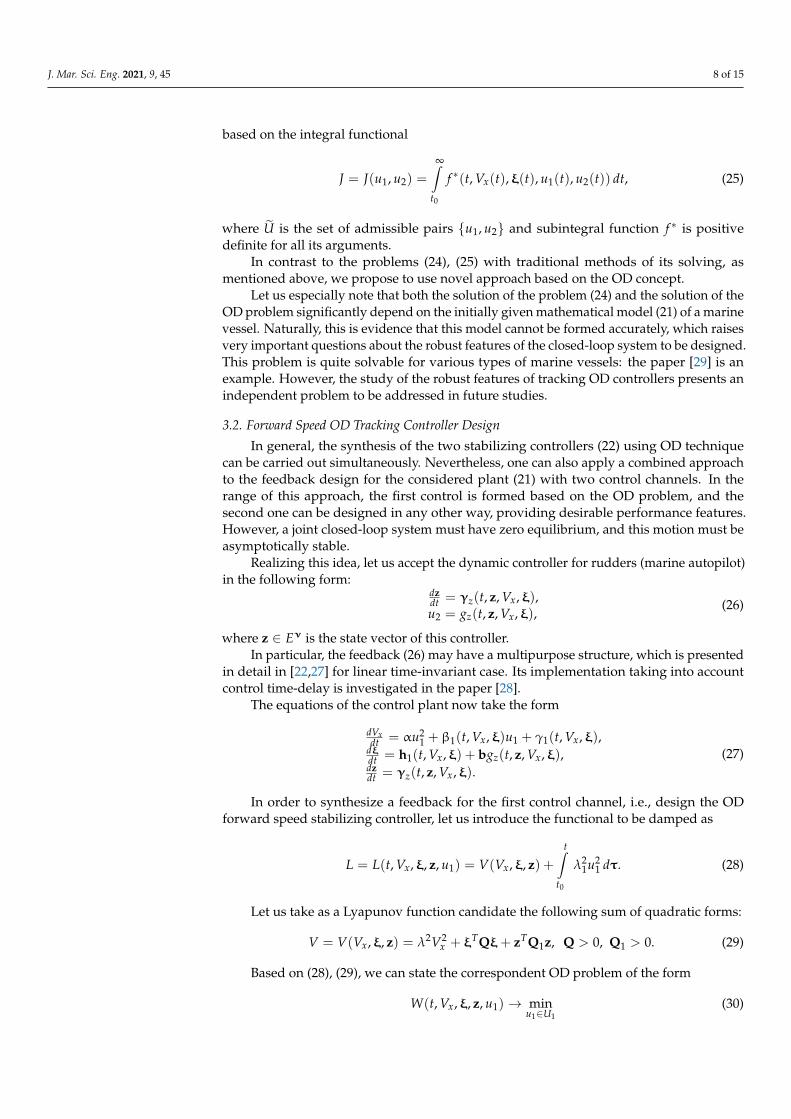
383 Figure 6. Rudders deflections )(tbδ=δ , )(tρδ , and )()()( ttt ρδ−δ=δ . 384

Figure 4. First control signals u1 = u1b(t), u1ρ(t), and u1(t) = u1(t)− u1ρ(t).

J. Mar. Sci. Eng. 2021, 9, x FOR PEER REVIEW 13 of 16

realized with the help of the designed tracking controllers. Initial conditions for all vari-375 ables are zero with the exception of forward speed and heading angle. By these variables, 376 the initial conditions smVx /4)0( = and 10)0( −=ϕ are accepted to distinguish them 377 from the reference motion. 378

0 50 100 150 200 250 3000

2

4

6

8

10

t (sec)

u 1 (m/s

)

u1b(t)

u1p(t)

0 50 100 150 200 250 300-1.5

-1

-0.5

0

0.5

1

t (sec)

u 1 (m/s

)

u1(t)

379 Figure 4. First control signals )(11 tuu b= , )(1 tu ρ , and )()()( 111 tututu ρ−= . 380

0 50 100 150 200 250 300

2

4

6

8

10

t (sec)

Vx (m

/s)

Vxb(t)

Vxp(t)

0 50 100 150 200 250 300

0

0.5

1

1.5

2

t (sec)

Vx (m

/s)

Vx(t)

381 Figure 5. Forward speed )(tVV xbx = , )(tVxρ , and )()()( tVtVtV xxx ρ−= . 382

0 50 100 150 200 250 300-10

0

10

20

30

40

t (sec)

δ (g

rad)

δb(t)

δp(t)

0 50 100 150 200 250 300

-2

-1

0

1

2

3

4

t (sec)

δ(gr

ad)

δ(t)

383 Figure 6. Rudders deflections )(tbδ=δ , )(tρδ , and )()()( ttt ρδ−δ=δ . 384

Figure 5. Forward speed Vx = Vxb(t), Vxρ(t), and Vx(t) = Vx(t)−Vxρ(t).

J. Mar. Sci. Eng. 2021, 9, 45 13 of 15

J. Mar. Sci. Eng. 2021, 9, x FOR PEER REVIEW 13 of 16

realized with the help of the designed tracking controllers. Initial conditions for all vari-375 ables are zero with the exception of forward speed and heading angle. By these variables, 376 the initial conditions smVx /4)0( = and 10)0( −=ϕ are accepted to distinguish them 377 from the reference motion. 378

0 50 100 150 200 250 3000

2

4

6

8

10

t (sec)

u 1 (m/s

)

u1b(t)

u1p(t)

0 50 100 150 200 250 300-1.5

-1

-0.5

0

0.5

1

t (sec)

u 1 (m/s

)

u1(t)

379 Figure 4. First control signals )(11 tuu b= , )(1 tu ρ , and )()()( 111 tututu ρ−= . 380

0 50 100 150 200 250 300

2

4

6

8

10

t (sec)

Vx (m

/s)

Vxb(t)

Vxp(t)

0 50 100 150 200 250 300

0

0.5

1

1.5

2

t (sec)

Vx (m

/s)

Vx(t)

381 Figure 5. Forward speed )(tVV xbx = , )(tVxρ , and )()()( tVtVtV xxx ρ−= . 382

0 50 100 150 200 250 300-10

0

10

20

30

40

t (sec)

δ (g

rad)

δb(t)

δp(t)

0 50 100 150 200 250 300

-2

-1

0

1

2

3

4

t (sec)

δ(gr

ad)

δ(t)

383 Figure 6. Rudders deflections )(tbδ=δ , )(tρδ , and )()()( ttt ρδ−δ=δ . 384 Figure 6. Rudders deflections δ = δb(t), δρ(t), and δ(t) = δ(t)− δρ(t).

Let us note that the dynamical quality of the presented transient process seems to bequite satisfactory. In addition, it is suitable to illustrate the dynamics of the closed-loopconnection under the action of sea wave external disturbance. Figure 7 shows the samecontrol process for the forward speed Vx, taking into account presence the approximaterepresentation of sea waves with an intensity of 5 on the Beaufort scale.

J. Mar. Sci. Eng. 2021, 9, x FOR PEER REVIEW 14 of 16

0 50 100 150 200 250 300

2

4

6

8

10

t (sec)

Vx (m

/s)

0 50 100 150 200 250 300

0

0.5

1

1.5

2

t (sec)

Vx (m

/s)

Vxb(t)

Vxp(t)

Vx(t)

385 Figure 7. Forward speed )(tVV xbx = , )(tVxρ , and )()()( tVtVtV xxx ρ−= under sea waves action. 386

Let us note that the dynamical quality of the presented transient process seems to be 387 quite satisfactory. In addition, it is suitable to illustrate the dynamics of the closed-loop 388 connection under the action of sea wave external disturbance. Figure 7 shows the same 389 control process for the forward speed xV , taking into account presence the approximate 390 representation of sea waves with an intensity of 5 on the Beaufort scale. 391

Finally, let us analyze the stability of the closed-loop system (17), (35), (41) with 392 synthesized tracking controllers. One can easily see that in order to provide aforemen-393 tioned analysis, it is sufficient to consider the zero-equilibrium stability for the 394 closed-loop system (27), (33) presented in deflections from the reference motion. 395

It is obvious that systems (27), (33) have zero equilibrium, and to investigate its sta-396 bility features, let us introduces the following Lyapunov function candidate: 397

xSxSξξx 122)( TT

xVVV =+λ== ,

λ=

S00

S2

1 ,

=

ξx xV

: . (42)

Here, the symmetrical matrix 0S > is a solution of the algebraic Riccati equation, 398 which is used in the range of LQR controller (37) synthesis: 399

−

−

−

−−−

=

98.222.197.2141.0

22.127.159.2102.0

97.259.204.7243.0

141.0102.0243.00107.0

S .

Let us notice that the introduced function )(xV satisfy the relationships 400

( ) ( ) ( )xxx 21 α≤≤α V , 5E∈∀x , (43)

with the following K-class functions: 401

( ) ( ) ( ) ( ) ,, 21max2

21min1 xSxxSx ⋅σ=α⋅σ=α

where 00115.0min =σ and 100max =σ are the minimum and maximum eigenvalues of 402 the matrix 1S , respectively. 403

Using the additional function ( ) K∈≡α xx3 , one can check if the following ine-404 quality is valid 405

( )xx 3)33(),27(

),( α−≤=dtdVtW , xBt ∈∀≥∀ x,0 , (44)

where xB is a box, determined by the relationships: 406

Figure 7. Forward speed Vx = Vxb(t), Vxρ(t), and Vx(t) = Vx(t)−Vxρ(t) under sea waves action.

Finally, let us analyze the stability of the closed-loop system (17), (35), (41) withsynthesized tracking controllers. One can easily see that in order to provide aforementionedanalysis, it is sufficient to consider the zero-equilibrium stability for the closed-loop system(27), (33) presented in deflections from the reference motion.

It is obvious that systems (27), (33) have zero equilibrium, and to investigate itsstability features, let us introduces the following Lyapunov function candidate:

V = V(x) = λ2V2x + ξTSξ = xTS1x, S1 =

(λ2 00 S

), x :=

(Vxξ

). (42)

Here, the symmetrical matrix S > 0 is a solution of the algebraic Riccati equation,which is used in the range of LQR controller (37) synthesis:

S =

0.0107 −0.243 −0.102 −0.141−0.243 7.04 2.59 2.97−0.102 2.59 1.27 1.22−0.141 2.97 1.22 2.98

.

J. Mar. Sci. Eng. 2021, 9, 45 14 of 15

Let us notice that the introduced function V(x) satisfy the relationships

α1(‖x‖) ≤ V(x) ≤ α2(‖x‖), ∀x ∈ E5, (43)

with the following K-class functions:

α1(‖x‖) = σmin(S1) · ‖x‖2, α2(‖x‖) = σmax(S1) · ‖x‖2,

where σmin = 0.00115 and σmax = 100 are the minimum and maximum eigenvalues of thematrix S1, respectively.

Using the additional function α3(‖x‖) ≡ ‖x‖ ∈ K, one can check if the followinginequality is valid

W(t, x) =dVdt

∣∣∣∣(27), (33)

≤ −α3(‖x‖), ∀t ≥ 0, ∀x ∈ Bx, (44)

where Bx is a box, determined by the relationships:

Bx(t) ={

x ∈ E5 : |xi| ≤ xim(t), i = 1, 5}

,

x1m(t) = 0.01Pρ|Vxρ(t)|, x2m(t) = 0.01Pρ∣∣Vyρ(t)

∣∣,x3m(t) = 0.01Pρ|ωρ(t)|, x4m(t) = 0.01Pρ|ϕρ(t)|,

x5m(t) = 0.01Pρ|δρ(t)| .

Here, the variable Pρ determines the relative width of the box Bx compared to thecurrent values of the reference signals. This variable was increased to such a value that thecondition (44) was met. The obtained value Pρ = 25% seems to be still admissible in therange of (43), (44) [4,5], determining the region of the local uniform asymptotic stability forthe reference motion, which is realized by tracking controllers (35), (41).

4. Discussion

The main goal of this work was to propose constructive methods for marine trackingcontrollers’ design taking into account the real conditions of a vessel’s motions. We focusedour main attention on a situation where the rudders’ deflections and the forward speed arepresented by initially given reference signals to be realized using tracking feedback controls.

This problem can be solved using different popular optimization approaches (Bell-man’s theory, MPC technique, sliding mode control, etc.). Nevertheless, we propose anew specific method for tracking controllers’ design, which ensures the desirable referencemotion of the vessel along the forward speed and heading angle.

This method is based on the optimal damping concept, which has certain advantagesrelated to the practical requirements for the dynamic features of a closed-loop connection.The main advantage of the aforementioned approach is that the numerical solution of theoptimization problems is essentially simplified. In contrast to well-known approaches [1–4],we applied OD tracking feedback as a control law with special features that allow it to beadjusted and implemented in real-time regime of motion.

The main result of this study is the development of the optimal damping concept toensure its practical applicability and effectiveness that is illustrated by a controller designfor a transport ship.

The investigations presented above could be further developed to consider the robustfeatures of the tracking control laws, information about the measurement noise, and thepresence of transport delays [24]. The results of the executed research could also beimplemented to provide desirable reference motion of the dynamic positioning systemsfor marine vessels [26,27]. Certain attention may be given to the multipurpose controllaws applications [22–25]. As for direct development of this study, it is possible to also useOD controller for the vertical rudders. The extension of the proposed approach to various

J. Mar. Sci. Eng. 2021, 9, 45 15 of 15

robotic systems is also of considerable interest. The scope of the proposed approach mayadditionally include remotely operated vehicles [11] and offshore structures [12].

Funding: This research was funded by the Russian Foundation for Basic Research (RFBR) controlledby the Government of Russian Federation, research project number 20-07-00531.

Acknowledgments: The author expresses his sincere gratitude to A.P. Zhabko for the interest to thetopic of this study and for the high-level professional suggestions.

Conflicts of Interest: The authors declare no conflict of interest.

References1. Fossen, T.I. Guidance and Control of Ocean Vehicles; John Wiley & Sons Ltd.: New York, NY, USA, 1994.2. Do, K.D.; Pan, J. Control of Ships and Underwater Vehicles. Design for Underactuated and Nonlinear Marine Systems; Springer: London,

UK, 2009.3. Jarjebowska, E. Model-Based Tracking Control of Nonlinear Systems; CRC Press, Taylor & Francis Group: Boca Raton, FL, USA, 2012.4. Khalil, H.K. Non-Linear Systems; Prentice Hall: Englewood Cliffs, NJ, USA, 2002.5. Slotine, J.; Li, W. Applied Nonlinear Control; Prentice Hall: Englewood Cliffs, NJ, USA, 1991.6. Fossen, T.I. Handbook of Marine Craft Hydrodynamics and Motion Control; John Wiley & Sons, Ltd.: New York, NY, USA, 2011.7. Reyes-Bayes, R.; Donaire, A.; van der Shaft, A.; Jayawardhana, B.; Perez, T. Tracking Control of Marine Craft in the port-

Hamiltonian Framework: A Virtual Differential Passivity Approach. In Proceedings of the 17th European Control Conference(ECC 2019), Naples, Italy, 25—28 June 2019; pp. 1636–1641.

8. Liu, Y.; Bu, R.; Gao, X. Ship Trajectory Tracking Control Systems Design Based on Sliding Mode Control Algorithm. Pol. Marit.Res. 2018, 25, 26–34. [CrossRef]

9. Guerreiro, B.J.; Silvestre, C.; Cunha, R.; Pascoal, A. Trajectory tracking nonlinear model predictive control for autonomous surfacecraft. IEEE Trans. Control. Syst. Techol. 2014, 22, 2160–2175. [CrossRef]

10. Hammound, S. Ship Motion Control Using Multi-Controller Structure. J. Marit. Res. 2012, 55, 184–190.11. Capocci, R.; Dooly, G.; Omerdi’c, E.; Coleman, J.; Newe, T.; Toal, D. Inspection-Class Remotely Operated Vehicles—A Review. J.

Mar. Sci. Eng. 2017, 5, 13. [CrossRef]12. Ramos, R.L. Linear Quadratic Optimal Control of a Spar-Type Floating Offshore Wind Turbine in the Presence of Turbulent Wind

and Different Sea States. J. Mar. Sci. Eng. 2018, 6, 151. [CrossRef]13. Roy, S.; Shome, S.N.; Nandy, S.; Ray, R.; Kumar, V. Trajectory Following Control of AUV: A Robust Approach. J. Inst. Eng. India

Ser. C 2013, 94, 253–265. [CrossRef]14. Ye, J.; Roy, S.; Codjevac, M.; Baldi, S. A Switching Control Perspective on the Offshore Construction Scenario of Heavy-Lift

Vessels. IEEE Trans. Control Syst. Technol. 2020, 29, 1–8. [CrossRef]15. He, W.; He, X.; Zoo, M.; Li, H. PDE Model-Based Boundary Control Design for a Flexible Robotic Manipulator With Input

Backlash. IEEE Trans. Control Syst. Technol. 2019, 27, 790–797. [CrossRef]16. He, W.; Gao, H.; Zhou, C.; Yang, C. Reinforcement Learning Control of a Flexible Two-Link Manipulator: An Experimental

Investigation. IEEE Trans. Syst. Man Cybern. Syst. 2020. [CrossRef]17. Lewis, F.L.; Vrabie, D.L.; Syrmos, V.L. Optimal Control; John Wiley & Sons, Ltd.: New York, NY, USA, 2012.18. Geering, H.P. Optimal Control with Engineering Applications; Springer-Verlag: Berlin/Heidelberg, Germany, 2007.19. Zubov, V.I. Oscillations in Nonlinear and Controlled Systems; Sudpromgiz: Leningrad, USSR, 1962. (In Russian)20. Zubov, V.I. Theory of Optimal Control of Ships and Other Moving Objects; Sudpromgiz: Leningrad, USSR, 1966. (In Russian)21. Zubov, V.I. Theorie de la Commande; Mir: Moscow, USSR, 1978.22. Veremey, E.I. Synthesis of multiobjective control laws for ship motion. Gyroscopy Navig. 2010, 1, 119–125. [CrossRef]23. Veremey, E.I. Dynamical Correction of Control Laws for Marine Ships’ Accurate Steering. J. Mar. Sci. Appl. 2014, 13, 127–133.

[CrossRef]24. Veremey, E.I. Optimization of filtering correctors for autopilot control laws with special structures. Optim. Control Appl. Methods

2016, 37, 323–339. [CrossRef]25. Veremey, E.I. Special Spectral Approach to Solutions of SISO LTI H-Optimization Problems. Int. J. Autom. Comput. 2019, 16,

112–128. [CrossRef]26. Veremey, E.I. Separate Filtering Correction of Observer-Based Marine Positioning Control Laws. Int. J. Control 2017, 90, 1561–1575.

[CrossRef]27. Sotnikova, M.V.; Veremey, E.I. Dynamic Positioning Based on Nonlinear MPC. IFAC Proc. Vol. (IFAC Pap.) 2013, 9, 31–36.

[CrossRef]28. Veremey, E.I.; Pogozhev, S.V.; Sotnikova, M.V. Multipurpose Control Laws Synthesis for Actuators Time Delay. J. Mar. Sci. Eng.

2020, 8, 477. [CrossRef]29. Chen, M.; Ge, S.S.; How, B.V.; Choo, Y.S. Robust adaptive position mooring control for marine vessels. IEEE Trans. Control Syst.

Technol. 2013, 21, 395–409. [CrossRef]