Risk sensitive asset allocation - UNSW Business SchoolPesaranandTimmermann(1995)examinedtherobust-ness of the evidence on predictability of US stock returns with respect to seven factors:dividendyield,earnings-priceratio,1monthT-billrate,12monthT-bill

Journal of Economic Dynamics & Control24 (2000) 1145}1177

Risk sensitive asset allocation

Tomasz R. Bielecki!,*, Stanley R. Pliska", Michael Sherris#

!Department of Mathematics, The Northeastern Illinois University, 5500 North St. Louis Avenue,Chicago, IL 60625-4699, USA

"Department of Finance, University of Illinois at Chicago, 601 S. Morgan St., Chicago,IL 60607-7124, USA

#Faculty of Commerce and Economics, University of New South Wales, Sydney, NSW 2052, Australia

Received 1 August 1998; accepted 14 April 1999

Abstract

This paper develops a continuous time modeling approach for making optimal assetallocation decisions. Macroeconomic and "nancial factors are explicitly modeled asGaussian stochastic processes which directly a!ect the mean returns of the assets. Weemploy methods of risk sensitive control theory, thereby using an in"nite horizonobjective that is natural and features the long run expected growth rate and theasymptotic variance as two measures of performance, analogous to the mean return andvariance, respectively, in the single period Markowitz model. The optimal strategy isa simple function of the factor levels, and, even with constraints on the portfolioproportions, it can be computed by solving a quadratic program. Explicit formulas canbe obtained, as is illustrated by an example where the only factor is a Vasicek-typeinterest rate and where there are two assets: cash and a stock index. The methods arefurther illustrated by studies of two data sets: U.S. data with two assets and up to threefactors, and Australian data with three assets and three factors. ( 2000 Elsevier ScienceB.V. All rights reserved.

JEL classixcation: G11; H20; C63

Keywords: Optimal asset allocation; Risk sensitive control

*Corresponding author.E-mail addresses: [email protected] (T.R. Bielecki), [email protected] (S.R. Pliska), m.sherris@

unsw.edu.au (M. Sherris).

0165-1889/00/$ - see front matter ( 2000 Elsevier Science B.V. All rights reserved.PII: S 0 1 6 5 - 1 8 8 9 ( 9 9 ) 0 0 0 1 7 - 2

1. Introduction

During recent years there has been a number of empirical studies providingevidence that macroeconomic and "nancial variables such as unemploymentrates and market-to-book ratios can be useful for forecasting returns for assetcategories. For example, Pesaran and Timmermann (1995) examined the robust-ness of the evidence on predictability of US stock returns with respect to sevenfactors: dividend yield, earnings-price ratio, 1 month T-bill rate, 12 month T-billrate, in#ation rate, change in industrial production, and monetary growth rate.Backtesting a simple switching strategy, they provided evidence that stockreturn predictability &could have been exploited by investors in the volatilemarkets of the 1970s'. In a more recent paper, Pesaran and Timmermann (1998)extended and generalized their "rst paper's recursive modeling strategy. Theyfocused their analysis on simulating &investors' search in the &real time' fora model that can forecast stock returns. Their new key idea was to divide the setof potential regressors into three categories expressing di!erent degrees offorecasting importance. Once again their "ndings provided evidence of predicta-bility of stock returns, this time in the UK's stock market, that can be exploitedby investors. Patelis (1997) concluded US excess stock returns can be predictedby looking at "ve monetary policy factors along with dividend yield, an interestrate spread, and the one-month real interest rate. Ilmanen (1997) showed thatthe excess returns of long term T-bond are a!ected by term spread, real yield,inverse wealth, and momentum factors. Furthermore, the bibliographies in thesepapers cite numerous additional, similar studies.

Some of these studies proceeded from their statistical conclusions to investi-gate whether return predictability can be exploited with dynamic investmentstrategies in order to achieve signi"cant pro"ts. All such investigations involvedbacktests of relatively simple, ad hoc trading rules. For instance, Ilmanen (1997)showed two dynamic strategies would have provided excess returns well inexcess of two benchmark static strategies. In one dynamic strategy the investoris long the T-bond if and only if its predicted excess return is positive.In the other, the position in the T-bond is proportional to the predicted excessreturn. This and other studies reinforce the view that dynamic asset allocationmodels which incorporate "nancial and economic factors can be useful forinvestors.

Meanwhile, there has been considerable research involving stochastic processmodels of assets combined with optimal consumption and/or investment deci-sions by economic agents. In some cases the models also include stochasticprocess models of factors. The famous study by Lucas (1978) has all theright elements: discrete time stochastic assets which are a!ected by factorlevels, a Markovian factor process, and economic agents who choose portfoliopositions and consumption levels so as to maximize the expected discountedutility of their consumption over an in"nite planning horizon. Merton (1971),

1146 T.R. Bielecki et al. / Journal of Economic Dynamics & Control 24 (2000) 1145}1177

Karatzas (1996), and other researchers used stochastic control theory to developcontinuous time portfolio management models where the assets are modeled asstochastic processes but "nancial and economic factors are ignored. Much morerelevant to the present paper is the one by Merton (1973), because he provideda continuous time asset management model featuring stochastic factors. Usingthe necessary conditions emerging from the dynamic programming functionalequation, he was able to establish some important "nancial economic principles.Merton's formulation was very general and abstract, and he did not provide anyexplicit calculations, concrete examples, or computational results.

Given Merton's groundwork and the empirical literature indicated above,one would logically expect there to be a large literature on continuous time,optimal portfolio management models which explicitly incorporate stochasticfactors and the mechanisms by which they a!ect asset returns, but the oppositeis the case. Apparently the theoretical and computational di$culties are toogreat. With the objective of either maximizing expected utility of terminal wealthor maximizing expected discounted utility of consumption over an in"niteplanning horizon, Merton's approach entails the solution of a partial di!erentialequation. However, explicit solutions are known only for a few special cases, andthe pde's can be solved numerically only for very small problems. Meanwhile,the implications of Merton's (1973) work for economic equilibrium have beeninvestigated in a variety of papers, among which the studies by Breeden (1979)and Cox et al. (1985) are noteworthy.

Kim and Omberg (1996), Canestrelli (1998), and Canestrelli and Pontini(1998) studied some simple, special cases of Merton's (1973) model where theinvestor's objective is to maximize expected (HARA or power) utility of wealthat a "xed, "nite date. They derived via a Riccati equation explicit solutions forthe value function and optimal trading strategy. Brennan and Schwartz (1996)and Brennan et al. (1997) studied a similar model, but they used numericalmethods to solve the dynamic programming functional equation (i.e., the Hamil-ton}Jacobi}Bellman partial di!erential equation) for the value function andoptimal trading strategy. But with only three factors, the pde has three statevariables and so they were already near the maximum that can be accommod-ated with a numerical approach.

Brandt (1998) and Campbell and Viceira (1999) worked directly with discretetime variations of Merton's (1973) model. Campbell and Viceira dealt witha model that is similar to Kim and Omberg's except that the investor's objectiveis to maximize expected utility of consumption over an in"nite planning hor-izon. Brandt (1998), also in discrete time, worked with the objective of maximiz-ing expected utility of consumption over a "nite planning interval. The set offeasible portfolio and consumption decisions was allowed to vary according toan observable forecasting process which, unfortunately, was not explicitly speci-"ed. Brandt developed a computational procedure involving the conditionalmethod of moments and the Euler equations that represent the "rst order

T.R. Bielecki et al. / Journal of Economic Dynamics & Control 24 (2000) 1145}1177 1147

optimality conditions. However, no proof was provided that this procedure isoptimal or even approximately optimal.

In short, the literature demonstrates that for concrete applications of Mer-ton's (1973) approach it is di$cult to obtain explicit characterizations of theoptimal strategies, even for simple models involving only a few factors. Andthese computational di$culties are not rescued by the modern approach whichavoids dynamic programming by using risk neutral probability measures (seeKaratzas (1996), Korn (1997), or Pliska (1986,1997)), because the inclusion ofstochastic factors means the resulting securities market model is incomplete (inthe sense of Magill and Quinzii (1996)). However, as will be argued in this paper,the computational di$culties can be ameliorated by adopting a new kind ofportfolio optimization objective or criterion.

The mathematical theory in this paper was introduced in Bielecki and Pliska(1999). Our model resembles the one developed by Merton (1973) in that factorsare modeled as stochastic processes which explicitly a!ect the asset returns.However, instead of maximizing the expected utility of terminal wealth or theexpected utility of consumption, the objective now is to maximize the portfolio'slong run growth rate adjusted by a measure of the portfolio's average volatility.This &risk sensitive' criterion corresponds to an in"nite horizon objective, and sothe optimal strategies are simpler, depending on the factor levels but not ontime. Moreover, the optimal strategies can be computed by solving simplequadratic programs, and so models with dozens or even hundreds of factors aretractable. An interesting feature of the theoretical results presented in Bieleckiand Pliska (1999) is that investment strategies that are optimal for the in"nitehorizon objective are universally optimal, i.e., they are optimal within any "niteplanning horizon for the type of asset allocation problems considered here.

It should be mentioned that the optimal strategies which emerge from our risksensitive dynamic asset management model resemble, at least for the case ofa single risky asset, the proportional strategies studied by Ilmanen (1997) andothers. Hence the ideas in this paper provide a sound, theoretical footing fordynamic investment strategies which previously have been selected only on anad hoc basis.

This paper is not the "rst to apply a risk sensitive optimality criterion toa "nancial problem. Lefebvre and Montulet (1994) studied a model for a "rm'soptimal mix between liquid and non-liquid assets; the calculus of variationsapproach was used to derive an explicit expression for the optimal division.Fleming (1995) used risk sensitive methods to obtain two kinds of asymptoticresults. In the "rst he considered a conventional, "nite horizon portfolio modeland studied certain limits as the coe$cient of risk aversion tends to in"nity. Inthe second he studied the long-term growth rate for conventional models withtransaction costs and HARA utility functions. Finally, Carino (1987) used risksensitive linear/quadratic/Gaussian control theory (see Whittle, 1990) to solvea particular discrete time, Lucas-type problem.


In summary, the purpose of this paper is to demonstrate that the risk sensitivedynamic asset management model of Bielecki and Pliska (1999) is a practical,tractable approach for making optimal asset allocation decisions. A preciseformulation of this model as well as the main results will all be found inSection 3. First, however, Section 2 will discuss and explain the risk sensitivecriterion that is a fundamental element of the model.

Section 4 is devoted to a special case of a simple asset allocation modelfeaturing a Vasicek type short interest rate and a stock index that is a!ected bythe level of interest rates. This example is completely solved; explicit formulas forthe optimal trading strategies and the optimal objective value are obtained. Inorder to develop understanding and economic intuition, the e!ects of individualparameters in these mathematical expressions are studied. Not only does thisexample illustrate the main ideas of Sections 2 and 3, but it will also be ofindependent interest to "nancial economists because it is one of the few modelsin the literature to provide explicit results and formulas for a concrete version ofMerton's (1973) model.

The Bielecki}Pliska methodology is further illustrated in the next two sec-tions where it is applied to two sets of monthly economic/"nancial data. InSection 5 the model is applied to US data, the same data that Brennan et al.(1997) studied. Section 6 is devoted to Australian data. In both cases thestatistical ability of our factors for forecasting asset returns is very limited, andyet the results are surprisingly good. This suggests that incorporation of betterfactors, such as those in the empirical studies cited above, would yield attractivestrategies for dynamic asset allocation.

2. The risk sensitive criterion

In order to introduce and explain the risk sensitive criterion, let <(t) denotethe time-t value of a portfolio and consider the measure of performance

lim inft?=

(1/c)t~1ln E(<(t))c, c(1, cO0.

This was used by Grossman and Zhou (1993) and Cvitanic and Karatzas (1994)to study a classical portfolio problem under a drawdown constraint. Note thatletting cP0 this becomes, in the limit, the same as the objective of maximizingthe portfolio's long-run expected growth rate (the Kelly criterion), whereas forc'1 it is not clear how to meaningfully interpret this criterion, although itresembles expected utility with an isoelastic or power utility function.

However, suppose this expression is rewritten as

Jh :"lim inft?=

(!2/h)t~1 ln Ee~(h@2)-/ V(t),


where h'!2, hO0, and where & :"' means &dexned as'. SubstitutingC(t)"ln<(t) enables one to establish a connection with the recently developedliterature on risk sensitive optimal control (e.g., see Whittle (1990)), where C(t)plays the role of a cumulative cost. This means that if we adopt, as we shall, theobjective of maximizing Jh, then many of the techniques that have recently beendeveloped for risk sensitive control can potentially be applied to our portfoliomanagement problem.

Moreover, as is well understood in the risk sensitive control literature,a power expansion [in powers of h, for h close to 0] of the quantity!2h lnEe~h

2 -/ V(t) yields

!

2

hln Ee~h

2 -/ V(t)"E ln<(t)!h4var(ln<(t))#O(h2), (2.1)

where O(h2) will typically depend on t. Hence Jh can be interpreted as thelong-run expected growth rate minus a penalty term, with an error that isproportional to h2. Furthermore, the penalty term is proportional to theasymptotic variance, a quantity that was studied by Konno et al. (1993) in thecase of a conventional, multivariate geometric Brownian motion model ofsecurities. The penalty term is also proportional to h, so h should be interpretedas a risk sensitivity parameter or risk aversion parameter, with h'0 and h(0corresponding to risk averse and risk seeking investors, respectively. Moreover,in the risk averse case maximizing Jh protects an investor interested in maximiz-ing the expected growth rate of the capital against large deviations of therealized rate from the expectations. The special case of h"0 will be referred toas the risk null case1, and note this is the same as the classical Kelly criterion,that is

J0"lim inf

t?=

t~1E ln<(t).

Some insight into the risk sensitive criterion can be obtained by consideringthe case where the process <(t) is a simple geometric Brownian motion withconstant parameters k and p. A simple calculation gives

Jh"k!1

2p2!

h4p2,

so the approximation mentioned above is, in this case, exact (which means thatthe term O(h2) is in fact equal to 0), with the asymptotic variance being preciselythe same as the square of the usual volatility.

1Whittle (1990) used the term risk neutral rather than risk null in this case. We chose the latterterminology in order to avoid a possible confusion with the term risk neutral used in the asset pricingcontext.


Additional insight about the risk sensitive criterion can be obtained bycomparing it with the objective under the classical single period Markowitzmodel. Ignoring the higher order terms and interpreting h as a Lagrangemultiplier, it is apparent that the problem of choosing a trading strategy so as tomaximize Jh is the same as maximizing the growth rate subject to a constraintthat the asymptotic volatility is equal to a "xed value. Hence maximizing Jh fora range of h will derive the &risk sensitive frontier', exactly analogous to thee$cient frontier in the Markowitz model. There are only two di!erences. First,the risk sensitive frontier lives in an asymptotic space corresponding to in"nitehorizon measures of mean return and variance rather than single periodmeasures. Second, the asymptotic frontier that is computed may not be exactlyequal to the true asymptotic frontier, due to the higher order terms in the Taylorseries expansion of Jh.

Naturally, if the investor has a very clear, speci"c planning horizon, then theexpected utility of terminal wealth should probably be maximized (assumingthat the results can be computed) and our risk adjusted performance measureshould not be used. However, for many important problems, especially themanagement of mutual funds, our risk adjusted growth rate criterion is ideal, forit captures both the portfolio's growth rate and the portfolio's average volatilityover an extended period of time.

3. Formulation of the model and the main results

We will develop a model consisting of m52 securities and n51 factors.Let (X, MF

tN,F, P) be the underlying probability space. Denoting by S

i(t) the

price of the ith security and by Xj(t) the level of the jth factor at time t, we

consider the following market model for the dynamics of the security prices andfactors:

dSi(t)

Si(t)

"(a#AX(t))idt#

m`n+k/1

pik

d=k(t), S

i(0)"s

i'0, i"1, 2,2,m,

(3.1)

dX(t)"(b#BX(t)) dt#K d=(t), X(0)"x, (3.2)

where=(t) is a Rm`n valued standard Brownian motion process with compo-nents =

k(t), X(t) is the Rn valued factor process with components X

j(t),

the market parameters a, A, R :"[pij], b, B, K :"[j

ij] are matrices of appro-

priate dimensions, and (a#Ax)i

denotes the ith component of the vectora#Ax.

Let h(t) denote an Rn valued investment process or strategy whose compo-nents are h

i(t), i"1,2,2,m.


Dexnition 3.1. An investment process h(t) is admissible if the following condi-tions are satis"ed:(i) h(t) takes values in a given subset s of Rm, and +m

i/1hi(t)"1, and

(ii) h(t) satis"es appropriate measurability and integrability conditions, as ex-plained in Bielecki and Pliska (1999).

The class of admissible investment strategies will be denoted by H.

Let now h(t) be an admissible investment process and consider the solution<(t) of the following stochastic di!erential equation:

d<(t)"m+i/1

hi(t)<(t)Cki

(X(t)) dt#m`n+k/1

pik

d=k(t)D, <(0)"v'0, (3.3)

where ki(x) is the ith coordinate of the vector a#Ax for x3Rn. The process<(t)

represents the investor's capital at time t, and hi(t) represents the proportion of

capital that is invested in security i, so that hi(t)<(t)/S

i(t) represents the number

of shares invested in security i, just as in, for example, Section 3 of Karatzas andKou (1996).

In this paper we shall investigate the following family of risk sensitizedoptimal investment problems, labeled as (Ph):

for h3(0,R), maximize the risk sensitized expected growth rate

Jh(v, x; h( ) )) :"lim inft?=

(!2/h)t~1ln Eh( > )[e~(h@2) -/ V(t)D<(0)"v,X(0)"x]

(3.4)

over the class of all admissible investment processes h( ) ),subject to Eqs. (3.2) and (3.3),

where E is the expectation with respect to P. The notation Eh( > ) emphasizes thatthe expectation is evaluated for the process<(t) generated by Eq. (3.3) under theinvestment strategy h(t).

Before we can present the main results pertaining to these investment prob-lems, we need to introduce the following notation, for h50 and x3Rn:

Kh(x) :" infh|s, 1{h/1

[(1/2)(h/2 #1)h@RR@h!h@(a#Ax)]. (3.5)

It is perhaps interesting to observe that Eq. (3.5) is a &local' optimizationproblem which amounts to maximization of the instantaneous return (i.e.,h@(a#Ax)) on the portfolio penalized by the portfolio's instantaneous volatility(i.e., the other term in Eq. (3.5)).


We also need to make the following assumptions:

Assumption (A1). The investment constraint set s satisxes one of the following twoconditions:(a) s"Rn, or(b) s"Mh3Rn: h

1i4h

i4h

2i, i"1,2,2,mN, where h

1i(h

2iare xnite constants.

Assumption (A2). For h'0,

lim@@x@@?=

Kh(x)"!R.

Assumption (A3). The matrix KK@ is positive dexnite.

Assumption (A4). The matrix RK@ equals 0.

Remark 3.1. (i) Note that if RR@ is positive de"nite and if Ker(A)"0, thenassumption (A2) is implied by assumption (A1)(a).

(ii) These assumptions are su$cient for the results below to be true, but, aswill be seen for the example considered in the next section, Assumption (A2) isnot necessary, in general.

(iii) Assumption (A4) says that the residuals of the factors are uncorrelatedwith the residuals of the assets. This assumption, which may be realistic for someapplications, but not for others, is discussed further in the concluding section.

Theorems 3.1}3.4, which were proved in Bielecki and Pliska (1999), contain keyresults that will be used in this paper.

Theorem 3.1. Assume (A1)}(A4) and xx h'0.Let Hh(x) denote a minimizing selector in Eq. (3.5), which means that Hh(x)

satisxes the following equation

Kh(x)"(1/2)(h/2 #1)Hh(x)@RR@Hh(x)!Hh(x)@(a#Ax).

Then the investment process hh is optimal for problem (Ph), where for all t50

hh(t) :"Hh(X(t)). (3.6)

Theorem 3.2. Assume (A1)}(A4), xx h'0, and consider problem Ph. Let hh(t) be asin Theorem 3.1. Then

(a) For all v'0 and x3Rn we have

Jh(v, x; hh( ) ))" limt?=

(!2/h)t~1 lnEhh( > )[e~(h@2) -/V(t)D<(0)"v, X(0)"x]

":o(h).


(b) The constant o(h) in (a) is the unique non-negative constant which is a part ofthe solution (o(h), v(x;h)) to the following equation:

o"(b#Bx)@gradxv(x)

!(h/4)n+

i,j/1

Lv(x)

Lxi

Lv(x)

Lxj

n`m+k/1

jikjjk#(1/2)

n+

i,j/1

L2v(x)

LxiLx

j

n`m+k/1

jikjjk

!Kh(x),

v(x)3C2(Rn), lim@@x@@?=

v(x)"R,

o"const., (3.7)

where gradxv(x) denotes the gradient of v(x).

The key point of the "rst equality in (a) is, of course, that the optimal objectivevalue is given by an ordinary lim rather than the lim inf as in Eq. (3.4). The keypoint of the second equality in (a) is that the optimal objective value doesnot depend on either the initial amount of the investor's capital (v) or onthe initial values of the underlying economic factors (x), although it depends,of course, on the investor's attitude towards risk (encoded in the value of h).The key point of (b) is that the optimal objective value is characterized in termsof the Eq. (3.7). The example in the next section illustrates how to solve thesystem (3.7).

Notice that in the preceding two theorems we had h'0. It remains toconsider the case corresponding to h"0. This is the classical problem ofmaximizing the portfolio's expected growth rate, that is, the growth rate underthe log-utility function (see, e.g. Karatzas, 1996). This problem, which will belabeled P

0, is exactly the same as Ph for h'0 except that now2

J0(v,x; h( ) )) :"lim inf

t?=

t~1Eh( > ) [ ln<(t)D<(0)"v, X(0)"x].

It turns out that to solve P0

it is necessary to make three additionalassumptions:

Assumption (B1). For each h50 the function Kh(x) (see Eq. (3.5)) is quadratic andof the form:

Kh(x)"(1/2)x@K1(h)x#K

2(h)x#K

3(h),

2This criterion comes about by setting h"0 in Eq. (2.1).


where K1(h), K

2(h), and K

3(h) are functions of appropriate dimension depending

only on h.

Assumption (B2). For each h50 the matrix K1(h) is symmetric and negative

dexnite.

Assumption (B3). The matrix B in Eq. (3.2) is stable.

Remark 3.2. (a) Assumption (B1) is satis"ed if, e.g. the matrix RR@ is non-singularand if s"Rn. As will be seen in the next section, non-singularity of RR@ is nota necessary condition for (B1) to hold.

(b) It follows from Section 5.5 in Bank et al. (1983) that limhs0Ki(h)"K

i(0) for

i"1, 2, 3.(c) Note the Assumption (B2) implies that Assumption (A2) is satis"ed.(d) Assumption (A1) was su$cient in the case h'0 in order to provide for

appropriate smoothness of the function Kh(x). Here, we make a strongerAssumption (B1) and therefore the Assumption (A1) is no longer needed.

Theorem 3.3. Assume (A3), (A4), and (B1)}(B3). Then the optimal strategy for P0

isas in Theorem 3.1 with h"0 and the optimal objective value o(0) is as in Theorem3.2(b) with h"0. Moreover, the optimal objective values for problems (Ph), h'0,converge to the optimal objective value for the risk null problem P

0when the

risk-aversion parameter converges to zero.

The next result characterizes the portfolio's expected growth rate under theoptimal investment strategy for the risk aversion level h'0; this will be used inthe next section where the motivation behind establishing this result will becomeapparent. We denote this growth rate by oh, which is to be distinguished fromthe optimal objective value o(h), as in Theorem 3.2.

Theorem 3.4. Assume (A3), (A4), and (B1)}(B3), xx h'0, let Hh(x) be as inTheorem 3.1, and suppose that Hh(x) is an azne function and that

lim@@x@@?=

[(1/2)Hh(x)@RR@Hh(x)!Hh(x)@(a#Ax)]"!R. (3.8)

Consider the equation

oh"(b#Bx)@ gradxvh,0(x)#(1/2)

n+

i,j/1

L2vh,0(x)

LxiLx

j

n`m+k/1

jikjjk

! [(1/2)Hh(x)@RR@Hh(x) ! Hh(x)@(a#Ax)],

vh,0(x)3C2(Rn), lim@@x@@?=

vh,0(x)"R,

oh"const. (3.9)


Then there exists a solution (oh, vh,0) to the preceding equation, the constant oh isunique, and we have

J0(v,x; hh( ) ))"oh (3.10)

for all (v, x)3(0,R)]Rn, where hh( ) ) is dexned as in Eq. (3.6).

4. Example: Asset allocation with Vasicek interest rates

In this section we present a simple example which not only illustrates the ideasdeveloped in the preceding sections, but also is of independent interest in its ownright. We study a model of an economy where the mean returns of the stockmarket are a!ected by the level of interest rates. Consider a single risky asset, saya stock index, that is governed by the stochastic di!erential equation

dS1(t)

S1(t)

"(k1#k

2r(t)) dt#p d=

1(t), S

1(0)"s'0,

where the spot interest rate r( ) ) is governed by the classical &Vasicek' process

dr(t)"(b1#b

2r(t)) dt#j d=

2(t), r(0)"r'0.

Here k1, k

2, b

1, b

2, p, and j are "xed, scalar parameters, to be estimated,

while=1

and=2

are two independent Brownian motions. We assume b1'0

and b2(0 in all that follows. We make no assumptions about the signs

of k1

and k2; readers looking for the risk premium to be constant should

expect k2"1, whereas we obtained k

2(0 in our empirical studies reported

below.The investor can take a long or short position in the stock index as well as

borrow or lend money, with continuous compounding, at the prevailing interestrate. It is therefore convenient to follow the common approach and introducethe &bank account' process S

2, where

dS2(t)

S2(t)

"r(t) dt.

Thus S2(t) represents the time-t value of a savings account when S

2(0)"1 dollar

is deposited at time-0. This enables us to formulate the investor's problemas in the preceding sections, for there are m"2 securities S

1and S

2, there

is n"1 factor X"r, and we can set b"b1, B"b

2, a"(k

1, 0)@, A"(k

2, 1)@,

K"(0, 0, j)@, and

R"Ap 0 0

0 0 0B.


With only two assets it is convenient to describe the investor's tradingstrategy in terms of the scalar valued function Hh(r), which is interpreted as theproportion of capital invested in the stock index, leaving the proportion1!Hh(r) invested in the bank account. We suppose for simplicity that there areno special restrictions (e.g., short sales constraints, borrowing restrictions, etc.)on the investor's trading strategy, so the investment constraint set s is taken tobe the whole real line.

In view of Theorem 3.1 the optimal trading strategy is easy to work out. With(see Eq. (3.5))

Kh(r)"infh|R

[(1/2) (h/2#1) (h, 1!h)RR@(h,1!h )@!(h,1!h) (a#Ar)],

it follows that the optimal trading strategy is hh(t)"[hI h(t),1!hI h(t)]@, wherehI h(t)"Hh(r(t)) and

Hh(r)"k1#k

2r!r

(h/2#1)p2, (4.1)

in which case

Kh(r)"!r!(k

1#k

2r!r)2

(h#2)p2.

It is interesting to note the obvious similarity between this optimal strategyand the well known results (see Merton (1971) or Karatzas (1996)) for the case ofconventional, complete models of securities markets and power utility functions.In particular, when k

2"0, so the mean returns of the stock market are

independent of the interest rates, the expressions for the trading strategies areidentical. Another special case of interest is when k

2"1, so that the &market risk

premium' (k1#k

2r!r)/p is constant. Here the results are somewhat boring, in

that Hh is constant with respect to r and Kh(r) is linear in r.More interesting is the study of o(h), our measure of performance under the

optimal trading strategy (see Theorem 3.2). In view of Eq. (3.7) this is obtained aspart of the solution (o, v) of the equation

o"1

2j2vA(r)#(b

1#b

2r) v@(r)!(h/4)j2(v@(r))2!Kh(r), (4.2)

where v is a unique (up to a constant) function satisfying lim@r@?=

v(r)"R. Tosolve this, we conjecture that a solution is obtained with v having the quadraticform

v(r)"ar2#br#c

for suitable constants a, b, and c. Substituting this and the expression forKh(r) into Eq. (4.2) and then collecting terms, we see that the quadratic terms


cancel out if and only if

j2ha2!2b2a!

(k2!1)2

(h#2)p2"0.

This quadratic equation in a has two roots, one of which is positive, while theother is negative. However, the requirement that lim

@r@?=v(r)"R is satis"ed

only for the positive root, so recalling our assumption that b2(0 it follows that

for the value of a we should take (for future purposes it is convenient to denotethe dependence on h and j)

a(h, j)"b2#Jb2

2#hj2(k

2!1)2/[(h#2)p2]

j2h. (4.3)

The linear terms on the right-hand side of Eq. (4.2) cancel if and only if thevalue of b is

b(h, j)"1#2k

1(k

2!1)/[(h#2)p2]#2b

1a(h, j)

Jb22#hj2(k

2!1)2/[(h#2)p2]

. (4.4)

Thus Eq. (4.2) does indeed have a solution with v as indicated; this solution isunique up to the constant c, the value of which does not matter. The value ofo(h, j) will then equal the remaining terms on the right-hand side of Eq. (4.2), i.e.

o(h, j)"j2a(h, j)#b1b(h, j)!

j2h[b(h, j)]2

4#

k21

(h#2)p2. (4.5)

Remark 4.1. Note that the above results are valid also in the case when k2"1.

The assumption (A2) is not satis"ed in this case since limr?~=

Kh(r)"R.

It is interesting to consider the risk null case, because here o(0) will turn out tobe the long-run expected growth rate under the strategy that is optimal whenh"0. Using L'Hospital's rule we compute the limits

a(0, j)"limhs0

a(h, j)"!

(k2!1)2

4b2p2

,

b(0,j)"limhs0

b(h, j)"b1(k

2!1)2

2b22p2

!

1

b2

!

k1(k

2!1)

b2p2

,

o(0,j)"limhs0

o(h, j)"!

b1

b2

#

[k1!(b

1/b

2)(k

2!1)]2

2p2!

j2(k2!1)2

4b2p2

.

(4.6)

Note that each of the three terms is non-negative. The Vasicek interest ratehas a limiting distribution with a mean equal to the so-called &mean reversion'


level !b1/b

2, which is the "rst term. The second term equals the contribu-

tion to the long-run expected growth rate due to trading in the stock index,assuming the interest rate is the constant mean reversion level. The thirdterm equals the contribution to the long-run expected growth rate due to thevolatility of the interest rate.

Another quantity of interest is the long-run expected growth rate whichresults from using the strategy hh(t) that is optimal for a particular value of h,a quantity that will be denoted by oh(j). Of course, o

0(j)"o(0, j), which is given

by Eq. (4.6), whereas for h'0 we use Theorem 3.4 and obtain the quantity oh(j)by solving for the constant o and the function v such that lim

@r@?=v(r)"R and

o"1

2j2vA(r)#(b

1#b

2r)v@(r)![(1/2)(Hh(r), 1!Hh(r))RR(Hh(r),

1!Hh(r))@!(Hh(r), 1!Hh(r))(a#Ar)]. (4.7)

We solve Eq. (4.7) in exactly the same way as Eq. (4.2), obtaining

oh(j)"!

b1

b2

#

2(h#1)

(h#2)2p2C[k1!(b

1/b

2)(k

2!1)]2!

j2(k2!1)2

2b2

D. (4.8)

Note that the second and third terms, respectively, of Eqs. (4.6) and (4.8) di!er bythe factor 4(h#1)/(h#2)2. This factor is strictly less than one for all h'0, soo(0, j)'oh(j) for all h'0. Thus the optimal expected growth rate when h"0 isgreater than when h is positive, as anticipated.

Remark 4.2. At this point we want to emphasize one more time that the mainadvantage of the risk-sensitive approach to dynamic asset allocation over theclassical log-utility approach is that the risk-sensitive approach provides anoptimal compromise between maximization of the capital expected growth rateand controlling the investment risk, given the investor's attitude towards riskencoded in the value of h. Even though the long-run expected growth rate of thecapital under h

0( ) ) is greater than under hh( ) ), if h'0, the asymptotic risk of

investment decreases with increasing values of h (see the discussion below, aswell as our numerical results that conclude this section).

Still another quantity of interest is (4/h)[oh!o(h)] which, by Eq. (2.1) can beinterpreted as an estimate of the asymptotic variance of ln<(t) under thestrategy that is optimal for the particular value of h. In general, this is a messyformula when expressed in terms of the original data; no simpli"cations seempossible. However, there is interest in computing o@(0, j) :"/

`o(h,j)/h Dh/0

, becausewhen h"0 the asymptotic variance under the optimal trading strategy will belimhs0 (4/h)[oh!o(h)]"!4o@(0, j). After lengthy, tedious calculations using


L'Hospital's rule and so forth, we obtained

o@(0, j)"!

[k1!(b

1/b

2)(k

2!1)]2

4p2

#

j2(k2!1)2

32b32p4

[j2(k2!1)2#4b2

2p2]

!

j24b2

2p4

[p2#k1(k

2!1)!(b

1/b

2)(k

2!1)2]2.

Note that each of the three terms is non-positive, as desired.Our various calculations can be reconciled with classical continuous time

optimal portfolio models (e.g., Merton, 1971; Karatzas, 1996) by consideringvarious limits as the data parameter jP0. This is because in the long-run whenj"0 the interest rate is essentially equal to the constant mean reverting value!b

1/b

2, in which case the drift coe$cient in the SDE for the stock index is the

constant k1!k

2b1/b

2. Hence, for instance, we have

limj?0

a(h, j)"!

(k2!1)2

2(h#2)b2p2

,

limj?0

b(h, j)"!

1

b2

!

2k1(k

2!1)!(b

1/b

2)(k

2!1)2

b2(h#2)p2

,

limj?0

o(h, j)"!

b1

b2

#

[k1!(b

1/b

2)(k

2!1)]2

(h#2)p2,

limj?0

oh(j)"!

b1

b2

#

2(h#1)[k1!(b

1/b

2)(k

2!1)]2

(h#2)2p2.

Note that when j"0 then our optimal strategy is the same as that whichemerges from the classical models when the objective is to maximize expectedutility of terminal wealth under a power utility function.

We now provide some numerical calculations that are intended to generatesome economic intuition about our asset allocation problem. Throughout weenvision time units in years and set b

1"0.05 and b

2"!1, so the mean

reverting interest rate is 5% per annum. We also set k1"0.1#(b

1/b

2)k

2so that

the stock index's drift coe$cient is always 0.1 whenever the interest rate is at themean reverting level. Finally, the volatility parameter for the stock index isalways taken to be p"0.2. Thus if the interest rate is "xed at the mean revertinglevel, then the stock index evolves like ordinary geometric Brownian motion andhas a long run expected growth rate equal of 8% per annum and an asymptoticvariance equal to 0.04.


Fig. 1. Rho(theta) for selected mean return sensitivities.

This leaves two unspeci"ed parameters: j and k2. For Figs. 1}3 we "x

j"0.02 and consider the e!ect of the interest rate sensitivity parameter k2.

Fig. 1 shows three graphs of the function o(h) corresponding to, from top tobottom, respectively, k

2"!1, k

2"0, and k

2"1. The numerical values are

expressed as percentages; the value of h varies between 0 and 6.0. Although thefunction o(h) involves the factor (k

2!1) raised to the "rst power, it turns out for

our chosen parameters that the value of o(h) when k2"1#d is not much

di!erent when k2"1!d, for all d'0 and h'0. Hence, roughly speaking, the

greater the sensitivity of the stock index risk premium (k1#k

2r!r)/p to the

interest rate, the greater the optimal objective value o(h).Fig. 2 shows three graphs of the function oh corresponding to, from top to

bottom, respectively, k2"!1, k

2"0, and k

2"1. It is interesting to compare

these values with 8%, the long run expected growth rate of the stock index itselfwhen the interest rate is "xed at the mean reverting level. Note that k

2enters the

equation for oh only as part of the factor (k2!1)2.

Fig. 3 shows three graphs of the estimated asymptotic variance correspondingto, from top to bottom, respectively, k

2"!1, k

2"0, and k

2"1. Plotted is

the quantity (4/h)[oh!o(h)], with oh and o(h)] expressed as percentages. It is


Fig. 2. Growth rate versus theta for selected mean return sensitivities.

Fig. 3. Asymptotic variance versus theta for selected mean return sensitivities.


interesting to compare these values with 4.0, the asymptotic variance for thestock index itself when the interest rate is "xed at the mean reverting level. Aswith oh, the estimated asymptotic variances are more sensitive to the value ofDk

2!1D than to the value of Dk

2D itself.

We also "xed k2"0 and studied the e!ect of the interest rate volatility

parameter j. We generated graphs of o(h), oh, and the estimated asymptoticvariances, respectively, for three di!erent values of j: 0, 0.02, and 0.04. Theresulting three graphs turned out to be qualitatively almost identical toFigs. 1}3, respectively, except that the curves labeled k

2"!1,0, and 1 should

be relabeled j"0.04, 0.02, and 0, respectively. In other words, with all three"gures, the bigger the value of j, the bigger the value of the correspondingfunction. Hence it seems that the greater the volatility of the interest rate,the greater the investment opportunities, although these opportunities will beaccompanied by greater volatilities.

5. Experiments with US data

In this section we backtest a two-asset model using data from the assetallocation study by Brennan et al. (1997). They had monthly data from January1974 to December 1994 for the T-bill short rate, a long term T-bond rate,the monthly returns for an index of US equities, and the dividend yields for thesame equity index. We augmented these data with similar numbers fromJanuary 1995 through November 1997. Our main objective for this and thefollowing section is to illustrate how to implement our risk sensitive assetallocation model.

A secondary objective for our empirical work is to see if risk sensitive tradingstrategies do better than more conventional ones, in spite of the fact that ourchoice of three factors is very poor for the purpose of predicting stock returns.When we regressed next month's returns against the three factors, the R2 andadjusted R2 turned out to be only 0.038 and 0.026, respectively. Moreover,although the coe$cients for the short rate and the dividend yield were statist-ically signi"cant at the 95% level, the intercept and the coe$cient for thelong rate were not signi"cant. On the other hand, Kandel and Stambaugh(1996) used a one-period optimization model for a Bayesian investor to concludethat weak regression results (such as ours) should nevertheless &exert asubstantial in#uence on the investor's portfolio decision'. If this is true ingeneral, then we should expect our risk sensitive strategies to outperformconventional ones.

We compare four kinds of trading strategies, each of which starts with $1000in January 1983. The data prior to 1983 were used for some of the strategies tomake initial estimates of parameters. First are the constant proportion strat-egies, where each month the division of wealth between the stock index and cash


Table 1Constant proportion strategies for US data

Stock Mean Volatility Sharpe Final Annualproportion return (%) (%) ratio wealth ($) turnover (%)

0.0 6.77 0.57 0.00 2,657 0.00.1 7.85 1.49 0.72 3,081 3.30.2 8.93 2.83 0.76 3,563 5.90.3 10.03 4.22 0.77 4,106 7.70.4 11.13 5.61 0.78 4,719 8.80.5 12.25 7.01 0.78 5,406 9.20.6 13.38 8.41 0.79 6,174 8.80.7 14.51 9.81 0.79 7,030 7.70.8 15.66 11.21 0.79 7,979 5.90.9 16.82 12.61 0.80 9,027 3.31.0 17.98 14.01 0.80 10,181 0.01.1 19.16 15.42 0.80 11,446 4.01.2 20.35 16.82 0.81 12,826 8.81.3 21.55 18.22 0.81 14,324 14.31.4 22.76 19.63 0.81 15,944 20.61.5 23.98 21.03 0.82 17,686 27.61.6 25.22 22.43 0.82 19,551 35.41.7 26.46 23.83 0.83 21,535 43.91.8 27.72 25.24 0.83 23,634 53.21.9 28.99 26.64 0.83 25,841 63.32.0 30.26 28.04 0.84 28,145 74.2

is rebalanced to a speci"ed proportion. Di!erent proportions were evaluated,ranging between 0 and 2.0. Table 1 shows for each proportion the correspondingportfolio's mean annual return, volatility, Sharpe ratio, "nal (November 1997)dollar value, and average annual turnover. The last measure is the percentage ofthe portfolio's value that is shifted between assets due to the rebalancing process;it is included in order to give some indication of the possible transaction costs.Fig. 4 shows a graph of the mean annual return versus the volatility for values ofthe stock proportion ranging from about 0.13 to about 1.50.

The second kind of trading strategies are 0-factor, risk sensitive strategies.These are the strategies resulting from our model when you take the matrixA"0 in Eq. (3.1). In particular, for the purposes of this section, this is the sameas taking k

2"0 in the Vasicek model of the preceding section. Consequently,

the optimal proportion (4.1) reduces to the well known formula resulting fromthe portfolio management problem where the investor's objective is to maximizeexpected iso-elastic utility of wealth at a speci"ed ("nite) planning horizon (seeMerton (1971), Karatzas (1996), and Eq. (41) of Kandel and Stambaugh (1996);the value of h depends in a simple way on the risk aversion parameter in the


Fig. 4. Mean return versus volatility for US data.

utility function). For this reason, our 0-factor risk sensitive strategies can also bethought of as classical, Merton-type stochastic control strategies.

In our backtesting experiment we are interested in whether the Merton-typestrategies fare better than the benchmark constant proportion strategies. If so,this would be evidence for the merits of the risk sensitive control approach(and stochastic control theory approaches, in general), irrespective of anyopportunity to use factors for predicting asset returns. This is because the factorlevels are ignored for the purpose of estimating the value of the parametersk1

and p. In particular, only the stock index returns prior to 1983 wereused for initial estimates of these two parameters. Moreover, each monthon a rolling basis the most recently observed return was added to the data setfor the purpose of updating the parameter estimates, and then the new portfolioproportions were computed from Eq. (4.1) and implemented. However, inorder to facilitate a comparison with the benchmark constant proportionstrategies described earlier, we imposed lower and upper bounds on thestock index proportion of 0 and 2.0, respectively. This means that if theproportion coming from expression (4.1) was lower (respectively, higher) than0 (resp. 2.0), then the proportion actually implemented during the monthwas 0 (resp. 2.0).

We backtested the 0-factor risk sensitive strategies for di!erent values of h, asshown in Table 2. Fig. 4 shows a graph of the mean return versus the volatility ash ranges from about 1 to 23.


Table 20-Factor risk sensitive strategies for US data

Mean Volatility Sharpe Final AnnualTheta return (%) (%) ratio wealth ($) turnover (%)

0 29.47 27.62 0.82 26,071 89.31 28.53 26.81 0.81 24,162 122.52 26.45 25.25 0.78 20,082 138.73 24.76 23.90 0.75 17,217 138.34 22.89 22.57 0.71 14,365 139.36 20.29 18.71 0.72 12,027 119.38 18.23 15.96 0.72 10,050 104.2

10 16.19 13.33 0.71 8,216 84.612 14.80 11.42 0.70 7,113 69.015 13.34 9.40 0.70 6,068 54.120 11.82 7.26 0.70 5,091 39.625 10.87 5.91 0.69 4,541 31.230 10.22 4.99 0.69 4,191 25.840 9.39 3.81 0.69 3,773 19.150 8.88 3.08 0.69 3,533 15.175 8.19 2.11 0.68 3,226 10.0

The third kind of strategy is our risk sensitive control strategy where the shortrate is the only factor, as in the preceding section. To backtest this kind ofstrategy we estimated p as for the 0-factor strategies, but now instead ofestimating k

1from just the sample of historical returns we estimated both k

1and

k2

by regressing in a rolling, month-to-month fashion the stock index returns ofprior months against the T-bill short rate at the beginning of the correspondingmonths. The parameters k

1and k

2were taken to be the regression intercept and

slope, respectively. This risk sensitive control strategy was backtested for di!er-ent values of h, as shown in Table 3. Fig. 4 shows a graph of portfolio meanreturn versus volatility as h ranges from about 2.5 to about 50.

Finally, the fourth kind of strategy we backtested is our risk sensitive controlstrategy where there are three factors: both interest rates and the stock indexdividend yield. We included this kind of strategy in spite of the fact that ourAssumption (A4) was violated in this case. In particular, although the residualsof the two interest rate factors are virtually uncorrelated with the residuals of thestock index, the residuals of the dividend yield factor are highly correlated withthe stock index residuals, just as one would anticipate. Nevertheless, we thoughtthere might be some interesting things to learn by proceeding with the backtestas if Assumption (A4) were realistic.

The backtest was conducted just like the backtest of the one factor, risksensitive strategies, only now the estimates of k

1and k

2(the latter now being

a 3-component vector) were updated each month by conducting a regression




0 28.86 27.43 0.81 24,492 123.11 28.30 26.76 0.80 23,563 151.32 28.02 25.97 0.82 23,528 177.03 27.14 25.12 0.81 21,912 196.94 25.85 24.15 0.79 19,469 199.96 23.13 22.05 0.74 15,215 205.38 20.49 19.05 0.72 12,232 197.2

10 17.80 16.25 0.68 9,432 175.912 15.99 14.16 0.65 7,855 154.215 14.27 11.70 0.64 6,600 123.620 12.53 9.04 0.64 5,470 92.225 11.44 7.37 0.63 4,832 73.530 10.70 6.22 0.63 4,426 61.240 9.75 4.74 0.63 3,941 45.750 9.17 3.84 0.63 3,663 36.575 8.39 2.61 0.62 3,309 24.4



0 28.60 20.60 1.06 31,550 484.71 27.18 19.64 1.04 27,461 499.72 25.55 18.48 1.02 23,375 506.13 23.86 17.45 0.98 19,585 490.44 22.01 16.34 0.93 16,059 473.26 19.55 14.30 0.89 12,403 429.08 16.81 12.16 0.83 9,125 379.7

10 15.03 10.28 0.80 7,472 332.512 13.88 8.84 0.80 6,564 291.115 12.59 7.28 0.80 5,645 240.320 11.25 5.63 0.79 4,790 186.225 10.41 4.60 0.79 4,311 152.030 9.83 3.88 0.79 4,005 128.440 9.10 2.97 0.78 3,640 98.050 8.64 2.42 0.77 3,430 79.275 8.03 1.68 0.75 3,160 53.6

with all three factors as independent variables. This kind of strategy was backtes-ted for di!erent values of h, as shown in Table 4. Fig. 4 shows a graph of eachportfolio's mean return versus its volatility as h ranges from about 0 to about 50.


In conclusion, it should be clear that it is easy to implement risk sensitivestrategies in a practical way. The continuous time theory is readily transformedto a discrete time context by proceeding on a rolling basis to use statisticalmethods for updating parameters, to use these updated parameters and newfactor values to compute new asset proportions, and to rebalance accordingly.On the other hand, it remains unclear from these preliminary experimentswhether risk sensitive strategies with underlying factors do better than moreconventional strategies, especially when transaction costs are considered. As canbe seen from Fig. 4, which ignores transaction costs, the 3-factor strategies didconsistently better than the others, by margins which are noteworthy at thehigher volatilities. On the other hand, the 0-factor and 1-factor risk sensitivestrategies did worse than the benchmark constant proportion strategies at alllevels of volatility. The performance of risk sensitive strategies will be discussedfurther in the following two sections.

6. Experiments with Australian data

In this section we back test some 3-asset, 3-factor risk sensitive strategies withmonthly Australian data from January 1981 to July 1997. The three assets arethe All Industrials index, the All Resources index (these are indexes of disjointsets of stocks), and cash. The three factors are the 90 day Australian bank billrate (which determines the short interest rate for the cash asset), the 10 yearAustralian Treasury bond rate, and the dividend yield for the All Ordinariesstock index.

We regressed each month's returns of the All Industrials against the month-beginning values of the three factors, giving R2"0.022 and only the interceptsigni"cant at the 95% level. In a similar regression of the All Resources,R2"0.047 and the intercept and two interest rate coe$cients were signi"cant atthe 95% level. Thus our ability to forecast returns of Australian stocks iscomparable to what it was for the US market.

We also conducted an (approximate) asymptotic test for the presence ofsample correlations between the residuals of the asset returns and the factorchanges. We thereby could not reject the null hypothesis of no correlationbetween the short interest rate changes and each of the two index residuals, soour Assumption (A4) is satis"ed if the short rate is the only factor. However, thecorrelations between the dividend yield changes and each of the two indexresiduals are signi"cantly negative, while the correlations between the 10 yearbond yield changes and the index residuals are negative at a much lower level ofsigni"cance. Hence our tests of strategies involving these last two factors mustbe viewed with caution.

In a fashion similar to what we did with our US data (see the precedingsection), we compared three kinds of strategies by doing backtests assuming the


Table 5Constant proportion e$cient frontier for Australia (proportions 50)

Proportion (%)Mean Volatility Sharpe Final Annual

Allindustrials

Allresources

Cash return(%)

(%) ratio wealth($)

turnover(%)

100 0 0 18.9 16.19 0.45 7,431 0.098.8 0 1.2 18.81 16 0.45 7,393 0.592.6 0 7.4 18.34 15 0.45 7,185 2.786.4 0 13.6 17.88 14 0.45 6,972 4.780.2 0 19.8 17.41 13 0.45 6,754 6.373.9 0 26.1 16.94 12 0.45 6,533 7.667.7 0 32.3 16.48 11 0.45 6,310 8.761.5 0 38.5 16.02 10 0.45 6,085 9.455.2 0 44.8 15.56 9 0.45 5,858 9.848.9 0 51.1 15.09 8 0.44 5,632 9.942.6 0 57.4 14.63 7 0.44 5,406 9.636.3 0 63.7 14.17 6 0.44 5,181 9.129.9 0 70.1 13.71 5 0.43 4,956 8.223.4 0 76.6 13.23 4 0.42 4,731 7.016.7 0 83.3 12.75 3 0.40 4,502 5.59.3 0 90.7 12.22 2 0.33 4,254 3.30 0 100 11.55 1.33 0.00 3,952 0.0

portfolios all start with $1000 in January 1985, using the data prior to 1985 forinitial estimates of the parameters, as necessary. We also considered two sets ofconstraints on the portfolio proportions: (1) all three proportions are non-negative (i.e., no short sales or borrowing) and (2) all three proportions aregreater than or equal to one (so, e.g. starting with a dollar you can borrowa dollar, go short one dollar in one index, and go long three dollars in the other).

For a benchmark we computed the e$cient frontier with respect to all feasibleconstant proportion strategies with monthly rebalancing. Of course this is a verytough benchmark, because a priori the investor will not know what proportionswill give rise to an outcome on the e$cient frontier. Nevertheless, we computedfor selected volatilities the feasible portfolio proportions that maximize themean annual return. The results for proportions 50 are given in Tables 5}7and for 51 in Tables 8}10. Tables 5 and 8 show the results for the two sets ofconstraints. Note that for the case of nonnegative proportions, the e$cientfrontier involves putting nothing in the All Resources, with all the funds dividedbetween cash and the All Industrials.

The second kind of strategies are the 0-factor risk sensitive strategies. Thesecorrespond to setting the matrix A"0 in Eq. (3.1), thereby giving riseto a geometric Brownian motion model for the pair of stock indexes. Just like


Table 60-Factor risk sensitive strategies for Australia (proportions 50)


0 18.12 15.68 0.42 6,905 56.91 18.76 15.23 0.48 7,453 54.92 18.74 14.89 0.49 7,488 56.03 18.59 14.55 0.49 7,412 56.94 18.40 14.27 0.48 7,302 57.16 18.31 13.89 0.49 7,273 54.88 18.08 13.63 0.48 7,134 52.9

10 17.82 13.39 0.47 6,966 49.412 17.63 13.22 0.46 6,844 44.415 17.61 12.30 0.50 6,961 41.320 17.10 10.79 0.52 6,764 43.725 16.14 9.48 0.49 6,203 41.030 15.36 8.13 0.48 5,788 34.440 14.44 6.28 0.47 5,325 25.550 13.88 5.15 0.46 5,047 20.275 13.12 3.65 0.45 4,677 13.4

Table 73-Factor risk sensitive strategies for Australia (proportions 50)


0 17.82 16.35 0.39 6,588 198.11 17.54 16.12 0.38 6,426 205.42 17.65 15.52 0.40 6,593 211.73 18.28 14.39 0.47 7,244 207.34 18.73 13.62 0.53 7,714 204.26 19.15 12.58 0.61 8,217 205.18 19.24 11.95 0.65 8,381 205.7

10 19.27 11.45 0.68 8,473 203.712 19.17 11.07 0.69 8,425 196.815 19.10 10.48 0.73 8,423 180.420 18.70 9.76 0.74 8,153 162.425 17.98 9.16 0.71 7,605 149.930 17.22 8.46 0.68 7,061 139.540 15.85 7.39 0.59 6,153 119.550 14.90 6.31 0.54 5,598 101.675 13.81 4.38 0.53 5,033 68.7

the 0-factor strategies that were described in the preceding section, the para-meters R and a here are estimated from the monthly returns by computingsimple sample means, variances, and covariances, and they are updated monthlyon a rolling basis. Then each month the updated parameters are substituted into


Table 8Constant proportion e$cient frontier for Australia (proportions 5!1)

Proportion (%)Mean Volatility Sharpe Final Annual

Allindustrials

Allresources

Cash return(%)

(%) ratio wealth($)

turnover(%)

300 !100 !100 30.1 36.76 0.50 10,813 182.6289.2 !89.2 !100 29.73 36 0.51 10,742 168.2269.8 !78.4 !91.4 28.66 34 0.50 10,702 141.0254 !73.4 !80.6 27.59 32 0.50 10,652 119.2238.1 !69.2 !68.9 26.53 30 0.50 10,513 99.4222.2 !64.6 !57.6 25.47 28 0.50 10,292 81.7206.4 !60.1 !46.3 24.43 26 0.50 10,001 66.0190.4 !55.4 !35 23.39 24 0.49 9,649 52.0174.6 !50.9 !23.7 22.36 22 0.49 9,247 40.0158.7 !46.2 !12.5 21.33 20 0.49 8,805 30.0142.8 !41.6 !1.2 20.32 18 0.49 8,331 22.3126.8 !37 10.2 19.31 16 0.49 7,836 20.6110.9 !32.4 21.5 18.31 14 0.48 7,327 19.895 !27.8 32.8 17.31 12 0.48 6,812 19.279 !23.2 44.2 16.32 10 0.48 6,297 18.463 !18.5 55.5 15.34 8 0.47 5,787 16.946.8 !13.8 67 14.35 6 0.47 5,287 14.430.3 !9 78.7 13.35 4 0.45 4,794 10.612.3 !3.8 91.5 12.27 2 0.36 4,279 4.9

Table 90-Factor risk sensitive strategies for Australia (proportions 5!1)


0 27.18 33.78 0.46 9,229 312.01 26.87 32.38 0.47 9,469 291.12 26.39 31.61 0.47 9,294 273.33 25.54 30.92 0.45 8,747 270.54 25.53 30.20 0.46 8,918 248.06 24.11 29.16 0.43 7,954 212.48 23.62 26.53 0.46 8,852 182.9

10 23.09 24.62 0.47 9,153 166.512 22.53 22.65 0.49 9,256 149.215 21.12 19.53 0.49 8,761 118.820 18.95 15.46 0.48 7,648 88.625 17.56 12.70 0.48 6,932 70.330 16.60 10.76 0.47 6,433 57.140 15.38 8.27 0.47 5,803 41.950 14.64 6.75 0.47 5,424 33.375 13.63 4.70 0.46 4,922 22.1


Table 103-Factor risk sensitive strategies for Australia (proportions 5!1)


0 30.19 36.55 0.51 11,267 937.51 32.75 32.95 0.65 17,941 910.72 32.47 30.43 0.69 19,384 868.23 32.47 28.62 0.73 20,759 822.34 32.24 27.13 0.76 21,416 784.16 31.64 24.95 0.81 21,693 689.78 30.53 23.10 0.82 20,584 601.3

10 29.59 21.66 0.84 19,541 542.312 28.07 20.43 0.81 17,365 493.015 25.50 18.60 0.75 14,029 444.720 21.93 15.99 0.65 10,284 368.625 19.83 13.39 0.62 8,683 305.530 18.51 11.32 0.62 7,811 256.140 16.82 8.68 0.61 6,745 192.750 15.79 7.05 0.61 6,132 154.575 14.40 4.87 0.60 5,353 103.2

the right-hand side of Eq. (3.5) in order to compute the portfolio proportions forthe coming month. The portfolio is rebalanced accordingly. These 0-factor risksensitive strategies were backtested for selected values of h and the two sets ofconstraints. The results are presented in Tables 6 and 9.

The third and "nal kind of strategies we backtested are 3-factor risk sensitivestrategies. The variances and covariances were estimated in the same way as wasdone for the 0-factor strategies, but the a vector and the A matrix in Eq. (3.1)were updated monthly by doing regressions. Again, the 3-factor proportionswere implemented monthly after computing the minimizing selector in Eq. (3.5).Thus our backtests of 3-factor strategies with Australian data were conducted inthe same general way that was done in the experiments with US data, asdescribed in the preceding section. The results for selected values of the riskaversion parameter h and for the two sets of constraints are displayed inTables 7 and 10.

In order to compare the three kinds of strategies, we constructed graphsshowing, for each kind of strategy, how the portfolio's mean annual returnvaried with respect to its volatility. Thus Fig. 5 shows three graphs, all forthe case where the portfolio proportions are required to be nonnegative.Fig. 6 shows a similar picture for the case where each proportion is only requiredto be greater than or equal to minus one (i.e., !100%). In both cases the3-factor risk sensitive strategies generally perform better than the 0-factor


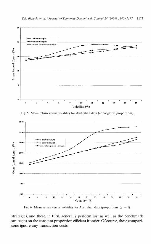
Fig. 5. Mean return versus volatility for Australian data (nonnegative proportions).

Fig. 6. Mean return versus volatility for Australian data (proportions 5!1).

strategies, and these, in turn, generally perform just as well as the benchmarkstrategies on the constant proportion e$cient frontier. Of course, these compari-sons ignore any transaction costs.


7. Discussion, 5nal remarks, and future research

In this paper we have shown how a risk sensitive criteria can be applied tooptimal asset allocation decision making. Expected returns are assumed to bedriven by speci"c factors, in this case interest rates and dividend yields. Theapproach developed takes advantage of any predictability in expected returnsarising from these factors. Expected returns on the asset classes are time varying.The optimal strategy is then determined using rolling regressions to estimatethe dynamics for asset returns. The risk sensitive criterion is based on in"nitehorizon measures of mean return and variance. In contrast to approaches toasset allocation using factor models currently in the literature, the risk sensitiveapproach readily allows the use of any number of factors and asset classes in theasset allocation optimisation.

The results from applying the approach to both USA and Australian data inbacktests are very encouraging. Using the mean-variance e$cient frontier asa basis for comparison of various strategies shows that dynamic strategiesoutperform constant proportion strategies and using factor models canprovide further enhancement in performance. Dynamic strategies lead to higherturnover and potentially higher transaction costs. This requires further invest-igation but use of futures rather than spot markets for physical assets, especiallyat the asset class level, will mean that transaction costs will be lower thanotherwise.

Throughout this paper we have been maintaining the assumption that resid-uals of the price processes and the residuals of the factor processes are notcorrelated. In terms of our model of Section 3, this assumption amounts torequiring that RK@"0. This assumption may or may not be reasonable, depend-ing upon the circumstances. For instance, based on the data that we collected forour empirical studies, with equities for assets this assumption is very reasonableif the short interest rate is the only factor, it is marginally reasonable ifa long-term interest rate is added as a factor, but it is clearly unreasonable ifdividend yield is added as a factor.

However, it is important to keep in mind that our assumption is not the sameas the assertion that changes in factor levels are uncorrelated with asset returns.This can be clearly seen by considering our Vasicek example. Suppose, forinstance, that the short rate is below the mean reversion level, a situation that isbullish for the stock. Then over a coming time interval the stock's return is likelyto be above average and the interest rate is likely to increase, and so our modelwill demonstrate a positive correlation between stock returns and interest ratemovements. This positive correlation exists in spite of our RK@"0 assumptionbeing satis"ed.

Nevertheless, it must be admitted it is very desirable to extend our presentmodel to cases where our RK@"0 assumption is not satis"ed. Presently ourtrading strategies do not account for interactions (correlations) between the


randomness underlying the price processes and the randomness underlying thefactor process, such as interactions one would "nd between the short rate factorand bonds with medium or long maturities. In general, if such interactions arenot negligible, then they will need to be accounted for in the optimal tradingstrategy via the so-called hedging term.

We shall brie#y illustrate this point by slightly extending the simple assetallocation model of Section 4. Speci"cally, consider the following extension ofthis model:

dS1(t)

S1(t)

"(k1#k

2r(t)) dt#p

1d=

1(t)#p

2d=

2(t), S

1(0)"s'0,

dr(t)"(b1#b

2r(t)) dt#j

1d=

1(t)#j

2d=

2(t), r(0)"r'0.

We conjecture (this will be studied in a future paper) that for this model theoptimal trading strategy is hh(t)"[hI h(t),1!hI h(t)]@, where hI h(t)"Hh(r(t)) and

Hh(r)"k1#k

2r!r

(h/2#1)p2#(h/2)

/@(r)(j1p1#j

2p2)

(h/2#1)p2,

and where the function /(r) is derived from an equation similar to (but morecomplicated than) Eq. (4.2). The second term in the above expression for Hh(r)hedges against the interactions between randomness underlying the price forma-tion block of the model, and the randomness underlying the factor dynamics.Note that in the model of Section 4 we postulated p

1"p, p

2"0, j

1"0, and

j2"j; this implies j

1p1#j

2p2"0, thereby eliminating the hedging term from

the formula for the optimal strategy. A challenging problem for future researchis to develop a model along these lines where interest rates of di!erent maturitiesare the factors and where there are "xed income asset categories correspondingto these same maturities.

Acknowledgements

We are grateful to M.J.P. Selby for helpful editorial suggestions.

References

Bank, B., Guddat, J., Klatte, D., Kummer, B., Tammer, K., 1983. Non-Linear Parametric Optimiza-tion. Birkhauser, Basel.

Bielecki, T.R., Pliska, S.R., 1999. Risk sensitive dynamic asset management. Journal of AppliedMathematics and Optimization 39, 337}360.


Brandt, M.W., 1998. Estimating portfolio and consumption choice: a conditional Euler equationsapproach. Working Paper. The Wharton School, University of Pennsylvania.

Breeden, D.T., 1979. An intertemporal asset pricing model with stochastic consumption andinvestment opportunities. Journal of Financial Economics 7, 265}296.

Brennan, M.J., Schwartz, E.S., 1996. The use of treasury bill futures in strategic asset allocationprograms. IFA Working Paper 229-1996. London Business School.

Brennan, M.J., Schwartz, E.S., Lagnado, R., 1997. Strategic asset allocation. Journal of EconomicDynamics and Control 21, 1377}1403.

Campbell, J.Y., Viceira, L.M., 1999. Consumption and portfolio decisions when expected returns aretime varying. Quarterly Journal of Economics 14(2) (May 1999) 433}495.

Canestrelli, E., 1998. Applications of multidimensional stochastic processes to "nancial investments.Working Paper. Dipartimento di Matematica Applicata ed Informatica, Universita &Ca' Foscari'di Venezia.

Canestrelli, E., Pontini, S., 1998. Inquiries on the applications of multidimensional stochasticprocesses to "nancial investments. Working Paper. Dipartimento di Matematica Applicata edInformatica, Universita &Ca' Foscari' di Venezia.

Carino, D.R., 1987. Multiperiod security markets with diversely informed agents. Ph.D. dissertation,Stanford University.

Cox, J.C., Ingersoll, J., Ross, S.A., 1985. An intertemporal general equilibrium model of asset prices.Econometrica 36, 363}384.

Cvitanic, J., Karatzas, I., 1994. On portfolio optimization under &drawdown' constraints, IMAPreprint No. 1224, University of Minnesota.

Fleming, W.H., 1995. Optimal investment models and risk sensitive stochastic control. In: Davis, M.,et al. (Eds.), Mathematical Finance. Springer, New York, pp. 75}88.

Grossman, S.J., Zhou, Z., 1993. Optimal investment strategies for controlling drawdowns.Mathematical Finance 3, 241}276.

Ilmanen, A., 1997. Forecasting U.S. bond returns. The Journal of Fixed Income, June,22}37.

Kandel, S., Stambaugh, R.F., 1996. On the predictability of stock returns: an asset allocationperspective. The Journal of Finance 51, 385}424.

Karatzas, I., 1996, Lectures on the Mathematics of Finance. American Mathematical Society,Providence, RI.

Karatzas, I., Kou, S.G., 1996. On the pricing of contingent claims under constraints. Annals ofApplied Probability 6, 321}369.

Kim, T.S., Omberg, E., 1996. Dynamic nonmyopic portfolio behavior. The Review of FinancialStudies 9, 141}161.

Konno, H., Pliska, S.R., Suzuki, K.I., 1993. Optimal portfolios with asymptotic criteria. Annals ofOperations Research 45, 184}204.

Korn, R., 1997. Optimal Portfolios. World Scienti"c, Singapore.Lefebvre, M., Montulet, P., 1994. Risk sensitive optimal investment policy. International Journal of

Systems Science 22, 183}192.Lucas, R.E., 1978. Asset prices in an exchange economy. Econometrica 46, 1429}1445.Magill, M., Quinzii, M., 1996. Theory of Incomplete Markets. The MIT Press, Cambridge,

MA.Merton, R.C., 1971. Optimum consumption and portfolio rules in a continuous time model. Journal

of Economic Theory 3, 373}413.Merton, R.C., 1973. An intertemporal capital asset pricing model. Econometrica 41, 866}887.Patelis, A.D., 1997. Stock return predictability and the role of monetary policy. The Journal of

Finance 52, 1951}1972.Pesaran, M.H., Timmermann, A., 1995. Predictability of stock returns: robustness and economic

signi"cance. The Journal of Finance 50, 1201}1228.


Pesaran, M.H., Timmermann, A., 1998. A recursive modelling approach to predicting UK stockreturns. Working Paper. Trinity College, Cambridge.

Pliska, S.R., 1986. A stochastic calculus model of continuous trading: optimal portfolios. Mathemat-ics of Operations Research 11, 371}384.

Pliska, S.R., 1997. Introduction to Mathematical Finance: Discrete Time Models. Blackwell,Oxford.

Whittle, P., 1990. Risk Sensitive Optimal Control. Wiley, New York.


Documents

Risk sensitive asset allocation - UNSW Business SchoolPesaranandTimmermann(1995)examinedtherobust-ness of the evidence on predictability of US stock returns with respect to seven factors:dividendyield,earnings-priceratio,1monthT-billrate,12monthT-bill