Embed Size (px)
Citation preview
Commodity Return Predictability ∗
Regina Hammerschmid†
University of Zurich
Swiss Finance Institute
October 30, 2017
ABSTRACT
The futures curve of an aggregate commodity portfolio is time-varying and changes from
upward (contango) to downward sloping (backwardation) which implies negative or positive
expected returns. The basis arises as a natural fundamental to predict commodity returns.
However, the empirical evidence on the aggregate portfolio level is very weak. I construct
a factor based on different forward rates along the futures curve and find that commodity
returns are predictable. Economic fundamentals, such as industrial production or global trade,
positively predict aggregate commodity returns and used jointly with this forward rates factor
significantly improve overall predictability in- and out-of-sample. I find evidence that expected
aggregate commodity returns are procyclical. When economic activity is high, the commodity
yield curve tends to be inverted and expected returns are high.
Keywords: Commodities, Return Predictability, Economic Fundamentals
JEL Classification: G11; G12; G17
∗I am grateful to Jens Jackwerth, Harald Lohre, Per Östberg, and Adriano Tosi for helpful comments.†Correspondence Information: University of Zurich, Plattenstrasse 32, 8032 Zurich, Switzerland;
I. Introduction
Expected returns of an aggregate commodity portfolio are driven by the shape of the under-
lying commodity yield curve which relates the current futures price to the spot price and the
remaining time to maturity. The futures curve changes from upward (contango) to downward
sloping (backwardation) which implies negative or positive expected returns on commodity fu-
tures. Figure 1 shows the significant extent to which the futures curve of an aggregate commodity
portfolio is time-varying. At the end of December 2008 the average futures price was increasing
with maturity and higher than the average spot price across 32 different commodities implying
an upward sloping yield curve (or contango). Conversely, at the end of April 2014 the commodity
yield curve was inverted (or in backwardation) which refers to a situation when average futures
prices are lower than the spot price. Interestingly, when looking at the economic activity around
these two dates, one finds that December 2008 was marked as a recession and April 2014 as an
expansionary period by the NBER business cycle dating.1 Further, the 12-month growth rate of
world industrial production was -11.16 % and 3.27 % respectively.
[Figure 1 about here.]
My main contribution is to show that aggregate commodity returns are predictable, both in-
and out-of-sample, using factors directly derived from the yield curve of an aggregate commodity
portfolio. Further, I find that the shape of the aggregate yield curve is strongly related to eco-
nomic activity and thus, I argue that expected commodity returns are procyclical. In contrast to
existing studies investigating individual commodity markets,2 I focus on the predictability of ag-
gregate returns similar to tradable commodity indices such as the SP-GSCI. Hong and Yogo (2012)
concentrate on the predictive power of futures’ markets open interest for aggregate commodity
returns and Gargano and Timmermann (2014) only investigate the predictability of aggregate
spot returns. Szymanowska, de Roon, Nijman, and van den Goorbergh (2014) document the
existence of spot and term risk premia in commodity futures returns. However, they do not pre-
dict aggregate returns, but instead aim to price different commodity risk factors. I contribute
to the literature by explicitly using information of the term structure of futures prices to predict
aggregate commodity returns and further relating it to economic fundamentals.
1For further information on NBER business cycle dates see http://www.nber.org/cycles.html2Gorton, Hayashi, and Rouwenhorst (2012) provide a good overview of individual commodity yield factors and
empirically test their predictability for commodity returns.
1
First, this paper examines whether returns of an aggregate commodity portfolio are pre-
dictable. No arbitrage implies that in contango (backwardation) futures prices are expected to
decrease (increase) and the roll yield is negative (positive). However, the main point is how to
best model the aggregate commodity yield curve and in particular its time-variation in order to
forecast future commodity returns. The basis, i.e. the difference between the current futures and
spot price, arises as a natural fundamental to predict returns on commodity futures. However, the
corresponding empirical evidence is very weak. I construct a factor which uses information along
the whole commodity futures curve. This forward rates factor significantly predicts commodity
futures returns across maturities and horizons. Further, I apply a principal component analysis
to the commodity basis of different maturities and I identify three factors which correspond to
the level, slope and curvature of the commodity yield curve. In particular, the curvature factor
significantly predicts commodity futures returns.
Second, this paper investigates how aggregate commodity returns relate to economic fun-
damentals. The focus is on rationalizing the time-variation of the commodity yield curve. I
document that economic fundamentals positively predict aggregate commodity futures returns
and using them jointly with these yield curve factors significantly raises overall predictability in-
and out-of-sample. Moreover, I find evidence that expected returns on commodity futures are
procyclical. When economic activity is high, the commodity yield curve tends to be inverted
and expected commodity returns are high. Hence, economic activity seems to be an important
determinant of an aggregate commodity portfolio’s yield curve.
I argue that the procyclical nature of expected commodity returns is driven by the time-
variation in industrial production where commodities are needed as production inputs. That is,
higher economic activity increases the demand for commodities as production inputs, which in
turn raises the spot price and reduces existing inventories. As a result, the commodity yield curve
gets inverted (backwardation) and expected returns on commodity futures are high and positive.
Conversely, a decrease in economic activity implies low expected commodity returns due to a
decrease in commodity demand and a fall in spot prices. Moreover, the analysis of commodity
sector returns shows that returns of commodities which are demanded as production inputs are
very sensitive to economic activity, whereas other commodities which are rather relevant for food
than industrial production are less affected by current economic conditions. These characteristics
2
translate to cross-sectional differences in marginal effects when using economic fundamentals to
predict future commodity sector returns.
This paper is structured as follows. Section II discusses different theories about the commodity
yield curve and their implications for return predictability. Section III describes the commodity
futures market data and the construction of the key predictor variables. In Section IV, I present
the main empirical results on the predictability of aggregate commodity returns as well as their
relation to economic fundamentals. Section V encompasses further empirical robustness analysis
and Section VI presents results on the predictability of commodity sector returns. Section VII
concludes.
II. Literature Review
The theory of storage states that the commodity futures price is a function of spot price,
storage costs and convenience yield (Working (1933), Kaldor (1939), Brennan (1958)).3 It is de-
rived from the cost-of-carry model and the no-arbitrage condition to price a commodity futures
contract. This theory postulates that commodity inventories react to changes in commodity sup-
ply and determine the shape of the futures curve. For example, in times of a commodity supply
surplus the spot price will decrease and inventories build up which implies that the storage costs
exceed the convenience yield. As a result the futures price will be higher than the spot price and
the futures curve upward sloping (contango). Conversely, a supply shortage will decrease inven-
tories and lead to an inverted futures curve (backwardation). Gorton, Hayashi, and Rouwenhorst
(2012) find empirical evidence that the level of physical inventories predict commodity futures
returns. Further, they show that the basis reflects the state of inventories and thus also predicts
returns.
In fact, the basis arises as a natural predictor for (individual) commodity returns. Fama and
French (1987) run classical regressions where they use the forward-spot spread, i.e. the basis,
to predict either futures returns or spot price changes. The empirical evidence for time-varying
expected returns depends on the type of commodity: it is strong for agriculturals and weak for
metals. Alternatively, Erb and Harvey (2006) and Fuertes, Miffre, and Rallis (2010) show that
a portfolio trading strategy which sorts on the basis—going long backwardated commodities and
3The convenience yield is the benefit one earns from physically holding the commodity to avoid stockouts orproduction disruptions.
3
shorting the ones in contango—can generate significant abnormal returns. In a similar vein,
Szymanowska, de Roon, Nijman, and van den Goorbergh (2014) find that the basis spread is a
significant risk factor which prices the cross-section of commodity returns. Yang (2013) shows
that investment shocks can explain the basis spread and thus provides a macroeconomic risk-based
explanation. Regarding the question of time-variation in the commodity yield curve, Bailey and
Chan (1993) identify idiosyncratic and common factors in the variability of the basis whose relative
importance depends on a commodity’s storability. They argue that macroeconomic fundamentals
cause common basis variability across different commodity markets.
According to the theory of normal backwardation commodity futures are used by hedgers to
transfer the price risk to speculators (Keynes (1930), Hicks (1939), Cootner (1960)). The inequal-
ity between short and long position of hedgers, which is known as hedging pressure, requires the
intervention of speculators to restore equilibrium in the futures market and hence, they demand
a risk premium as compensation. This theory postulates that the hedging pressure of commodity
producers and consumers determines the shape of the futures curve. For example, if hedgers are
net short, speculators must be net long. Since the latter demand positive expected returns on
their long positions, the futures price will be lower than the spot price and the commodity market
is in backwardation. Conversely, if hedgers are net long, speculators will demand positive returns
on their short positions which implies an upward sloping futures curve (contango). Empirically
the hedging pressure can predict returns on individual (mostly agricultural) commodity futures
(Chang (1985), Bessembinder (1992), de Roon, Nijman, and Veld (2000)).
These theories focus on futures prices of individual commodities and the resulting character-
istics can explain the cross-sectional differences in commodity returns. However, it is not obvious
how these individual yield factors affect the futures curve and returns on an aggregate commodity
portfolio.4 Idiosyncratic effects probably average out and the focus of this paper is on common
time-series variation instead of cross-sectional heterogeneity. In a similar vein, Hong and Yogo
(2012) show that open interest in futures markets is a better predictor for aggregate returns than
the hedging pressure or the basis, which holds true for different asset classes. They argue that
open interest contains information about future economic activity which is not fully revealed by
4For example, the role of inventories is different for perishable or non-perishable commodities. While perishablegoods cannot be stored and have a high convenience yield, non-perishable commodities will cause higher storagecosts. Similarly, the hedging pressure for agriculturals will be strongly influenced by seasonality or wheather risk,whereas these factors are less important for commodities that can be produced throughout the year.
4
prices alone, since asset prices initially underreact to macroeconomic news. In line with the results
in this paper, they find that expected commodity returns are procyclical. However, Hong and
Yogo (2012) do not relate their results to the term structure of futures prices. Open interest is a
transaction quantity which might not contain the same information as an aggregate yield curve.
Furthermore, there is little evidence how economic fundamentals, such as global trade or
industrial production, affect the time-series variation in aggregate commodity returns. Gargano
and Timmermann (2014) use some macroeconomic variables to predict commodity spot returns.
However, their focus is more on out-of-sample predictability and multivariate approaches, rather
than on rationalizing the cyclical properties of aggregate commodity futures returns. Still, the
relation of commodity returns to economic fundamentals might be important for producers who
want to hedge future price risk, as well as financial investors who expect positive returns on their
commodity portfolios. In this vein, the objective of this paper is to understand how a sudden
decrease in global trade or industrial production affects the average pricing of commodities.
III. Data and Variable Definitions
The aggregate commodity portfolio consists of 32 different commodities spread across 5 sectors
(Energy, Grains and Oilseeds, Livestock, Metals, Softs) and covers a broad commodity market
universe. For each commodity, I collect daily settlement prices of all individual futures contracts
available on Bloomberg. I select only liquid contracts by neglecting those contracts with zero
trading volume for at least one year prior to expiration. Table I lists all commodities grouped by
sector together with the exchange on which they are traded, the corresponding Bloomberg ticker
symbol, the year of the first recorded observation and the delivery months used. The data set
is comparable to the ones used by Gorton, Hayashi, and Rouwenhorst (2012), Hong and Yogo
(2012) and Szymanowska, de Roon, Nijman, and van den Goorbergh (2014). I choose January
1975 as the starting date since price data for nearly half of the 32 commodities is available from
this date onwards. The sample period ends in August 2015.
Data on open interest, i.e. the quantity of futures contracts outstanding, as well as long and
short positions of commercial traders (hedgers) for each futures contract is published in the Com-
mitment of Traders reports issued by the Commodity Futures Trading Commission (CFTC). The
corresponding CFTC codes for each individual commodity are listed in the last column of Table I.
5
Note that the CFTC data starts in January 1986. Further, I use data on trading volume for each
commodity futures contract which is also taken from Bloomberg. As proxies for economic funda-
mentals I use monthly OECD aggregate data for industrial production, total exports and imports
as well as the composite leading indicator and business confidence index.5 Since commodities
are traded worldwide, I choose OECD aggregate variables instead of macroeconomic variables for
individual countries. Data on economic fundamentals is from the OECD database and starts in
January 1975, except for data on exports and imports which is only available since January 1980.
A. Commodity returns
The h-month return of a fully collateralized long position in a commodity futures contract
with maturity T in excess of the risk-free rate is
rx(n)t+h =
Ft+h,T − Ft,T
Ft,T(1)
where Ft,T is the futures price at the end of month t which matures at the end of month T . I
assume that at time t, Ft,T is invested as collateral at the risk-free rate and hence, the futures
position is fully collateralized. Individual futures contracts are rolled over to the next maturity
contract n = T − t months before delivery. The roll-over is done end of month and prices are
backwards ratio adjusted. To analyze the term structure of returns, I calculate returns with
different times to maturity and use n = 1, 2, 3, 4 months before delivery to roll over each contract
to the next nearest contract. Further, I calculate returns over various holding periods, where
h = 1, 3, 6, 9, 12 months, to analyze the effect of different forecasting horizons.
First, I calculate h-month returns with maturity n, rx(n)t+h, for each individual commodity.
Second, I calculate an equal weighted average return within each sector and third, I equal weight
each sector return to obtain the return on an aggregate commodity futures portfolio. As a result no
sector will dominate even if the number of commodities within each sector varies over time. Panel
A of Table II reports summary statistics for the 1-month aggregate commodity returns across
different maturities. The average monthly excess return of this aggregate commodity portfolio
is nearly 30 basis points with a monthly volatility of well over 3 %. Moreover, these returns are
5The OECD composite leading indicator aggregates various economic variables of all OECD countries and isconstructed to anticipate economic turning points around 6 to 9 months ahead.
6

negatively skewed, have a kurtosis of over 5 and very low first-order autocorrelations. Overall,
there is little unconditional variation between returns of different maturities. In addition to the
statistics reported in Table II, the correlation between these monthly aggregate commodity returns
and the SP-GSCI index returns is 0.8, and 0.92 with the DJ-UBS commodity index, respectively.
B. Predictor variables
The predictor variables are divided into three groups. The first group consists of commodity
fundamentals which directly relate to the futures curve. The second group comprises additional
commodity-specific variables such as hedging pressure or open interest growth in the futures
market. The third group contains economic fundamentals.
B.1. Commodity fundamentals
The basis or forward-spot spread relates the current futures price to the spot price. The
n-month basis of a commodity future is given by
basis(n)t =
(
Ft,T
St
)1
(T −t)
− 1 (2)
where n = T − t = 1, 2, 3, 4 months before delivery. For the spot price St, I use the nearest-to-
maturity futures contract. The basis is positive if the commodity market is in contango (upward
sloping yield curve) and negative in times of backwardation (downward sloping yield curve).
Alternatively, the forward rate relates two futures prices with different maturities. The n-
month forward rate of a commodity future is defined as
forward(n)t =
(
Ft,T
Ft,T −1
)
− 1 (3)
where forward(1)t = basis
(1)t holds and n = T − t = 1, 2, 3, 4 months before delivery. For longer
maturities, the forward rate corresponds to a linear interpolation of the futures curve.
First, I calculate the basis and forward rates for each individual commodity and for different
maturities, with n = 1, 2, 3, 4 months to delivery. To aggregate within sectors I use the median
basis and median forward rates, which is less sensitive to outliers. Across sectors I compute
equally weighted averages of sector basis and sector forward rates, similar to Hong and Yogo
7
(2012). Panel A of Table II also reports summary statistics for the aggregate commodity basis
and forward rates across different maturities. The average basis over the whole sample period from
1975 to 2015 is positive which implies that the commodity market was on average in contango.
However, the basis volatility indicates quite some time-series variation. Overall, the basis and
forward rates across different maturities seem to be highly correlated since there is little variation
across the unconditional moments. Figure 2 shows a time-series plot of the aggregate commodity
basis with maturity 1 and 4 months. At first glance, there is a substantial amount of variation
both across time and across maturities with some significant spikes. In general, the basis tends
to be in contango during turbulent economic times, such as the oil crises in the late 1970s or the
recent financial crisis.
[Figure 2 about here.]
To explain common time-series variation in the term structure of the aggregate commodity
basis, I apply a principal component analysis to the basis of different maturities. The first three
principal component factors explain nearly 99 % of basis variation.6 Figure 3 shows the loadings of
each individual PC factor. Obviously, the first factor captures the average level of the basis across
maturities. The second factor negatively loads on the short-end and positively on the long-end of
the commodity yield curve and thus, represents the slope of the futures curve. The third factor is
dominated by the negative loading of the 2-month basis which seems to drive the curvature of the
commodity yield curve. The fourth PC factor is rather irrelevant in explaining basis variation.
[Figure 3 about here.]
B.2. Additional predictors
Besides commodity fundamentals, there are other variables known to predict commodity re-
turns. First, I calculate the volatility of commodity returns as the standard deviation of daily
returns over the past 12 months. Second, I use commodity spot price changes which are equal to
futures returns at expiration, i.e. with zero months to maturity. For both variables, the return
volatility as well as spot price changes, I first equally weight within each sector and then, equally
weight across sectors to get aggregate versions of each variable.
6The first PC factor explains 84 %, the second 11 % and the third about 4 % of basis variation.
8
Hedging pressure is a measure of supply and demand imbalances in the commodity futures
market. It is defined as the ratio of the difference between the number of short and long hedge
positions held by commercial traders relative to the total number of hedge positions held by
commercial traders in a specific commodity futures market. To aggregate within each sector, I
sum all individual short and long positions across all commodities in that sector and calculate
the sector hedging pressure. Then I compute the aggregate commodity market hedging pressure
as an equally weighted average of sector hedging pressures, similar to Hong and Yogo (2012).
Open interest in a specific commodity market is defined as the total number of futures contracts
outstanding. Similarly, trading volume is defined as the total number of futures contracts traded
on a day and in a specific commodity market. For both variables, I first aggregate within each
sector by summing the total number of futures (outstanding or traded) across all commodities
in that sector. Next, I calculate monthly growth rates of sector open interest and sector volume.
Finally, the aggregate growth rate of commodity market open interest or volume is an equally
weighted average of growth rates for each sector. Following Hong and Yogo (2012), I smooth
these monthly growth rate series by taking a 12-month geometric average within each time series
which are then referred to commodity market open interest or commodity market volume.
Panel B of Table II reports summary statistics for these additional commodity specific pre-
dictor variables. Note that the sample period for these variables is restricted to January 1986
to August 2015 because of the CFTC data availability. The average 12-month volatility of daily
commodity futures returns is about 25 % and the average spot price change is 60 basis points
which is twice as high as the average futures returns with higher maturity. The average hedging
pressure is significantly positive which implies that on average hedgers in the commodity market
are net short. Further, total open interest and trading volume in the aggregate commodity fu-
tures market is growing, since the average 12-month growth rate of open interest is 0.7 % and the
average 12-month growth rate of trading volume is 1.52 %.
B.3. Macroeconomic variables
The last group contains different economic fundamentals, namely OECD aggregate industrial
production (IP), total exports (EXP) and imports (IMP), the composite leading indicator (CLI)
and the business confidence index (BCI). For all 5 variables, I calculate monthly growth rates
and corresponding summary statistics are reported in Panel C of Table II. The monthly growth
9
rate of industrial production has a mean of 0.17 % implying that total OECD output is slowly
growing over time. Total exports and imports are growing as well with an average growth rate
of 0.56 % and 0.65 %, respectively. In contrast, the average monthly changes of the composite
leading indicator as well as the business confidence index is basically zero. The latter observation
is expected because the indicators are detrended.
IV. Empirical Results
The first part of the empirical analysis addresses the question whether returns of an aggregate
commodity portfolio are predictable. The focus is on testing the predictive power of three different
measures derived from the commodity yield curve, namely the basis, the forward rates and the
PC-factors extracted from the basis. The second part examines the relation between aggregate
commodity returns and economic fundamentals. I investigate how commodity returns as well as
the commodity yield curve vary with economic activity.
A. Predicting aggregate commodity returns
A.1. Basis regressions
The first variable to predict returns of a portfolio of commodity futures is an aggregate version
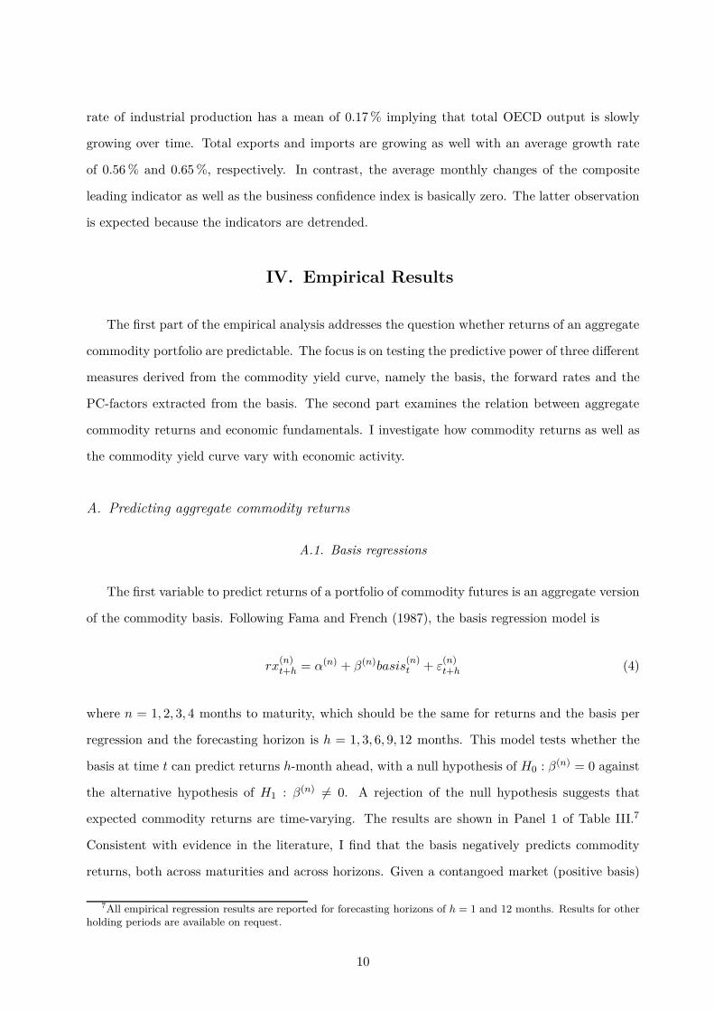
of the commodity basis. Following Fama and French (1987), the basis regression model is
rx(n)t+h = α(n) + β(n)basis
(n)t + ε
(n)t+h (4)
where n = 1, 2, 3, 4 months to maturity, which should be the same for returns and the basis per
regression and the forecasting horizon is h = 1, 3, 6, 9, 12 months. This model tests whether the
basis at time t can predict returns h-month ahead, with a null hypothesis of H0 : β(n) = 0 against
the alternative hypothesis of H1 : β(n) 6= 0. A rejection of the null hypothesis suggests that
expected commodity returns are time-varying. The results are shown in Panel 1 of Table III.7
Consistent with evidence in the literature, I find that the basis negatively predicts commodity
returns, both across maturities and across horizons. Given a contangoed market (positive basis)
7All empirical regression results are reported for forecasting horizons of h = 1 and 12 months. Results for otherholding periods are available on request.
10
the futures price is thus expected to fall, or alternatively, if the futures market is in backwardation
(negative basis) expected returns are positive, which is in line with the expected behaviour of the
roll yield. However, the statistical evidence for the predictive power of the commodity basis on
the aggregate level is very weak. The only slope coefficient which is significant at the 10 % level
is found for the 2-month maturity and 1-month forecasting horizon.8
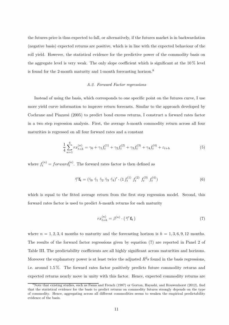
A.2. Forward Factor regressions
Instead of using the basis, which corresponds to one specific point on the futures curve, I use
more yield curve information to improve return forecasts. Similar to the approach developed by
Cochrane and Piazzesi (2005) to predict bond excess returns, I construct a forward rates factor
in a two step regression analysis. First, the average h-month commodity return across all four
maturities is regressed on all four forward rates and a constant
1
4
4∑
n=1
rx(n)t+h = γ0 + γ1f
(1)t + γ2f
(2)t + γ3f
(3)t + γ4f
(4)t + εt+h (5)
where f(n)t = forward
(n)t . The forward rates factor is then defined as
γ̂′ft = (γ̂0 γ̂1 γ̂2 γ̂3 γ̂4)′ · (1 f(1)t f
(2)t f
(3)t f
(4)t ) (6)
which is equal to the fitted average return from the first step regression model. Second, this
forward rates factor is used to predict h-month returns for each maturity
rx(n)t+h = β(n) ·
(
γ̂′ ft
)
(7)
where n = 1, 2, 3, 4 months to maturity and the forecasting horizon is h = 1, 3, 6, 9, 12 months.
The results of the forward factor regressions given by equation (7) are reported in Panel 2 of
Table III. The predictability coefficients are all highly significant across maturities and horizons.
Moreover the explanatory power is at least twice the adjusted R2s found in the basis regressions,
i.e. around 1.5 %. The forward rates factor positively predicts future commodity returns and
expected returns nearly move in unity with this factor. Hence, expected commodity returns are
8Note that existing studies, such as Fama and French (1987) or Gorton, Hayashi, and Rouwenhorst (2012), findthat the statistical evidence for the basis to predict returns on commodity futures strongly depends on the typeof commodity. Hence, aggregating across all different commodities seems to weaken the empirical predictabilityevidence of the basis.
11
indeed predictable when considering information along the whole futures curve instead of just one
specific tenor point. Importantly this forward rates factor is the same for all regressions, meaning
that a single linear combination of forward rates forecasts aggregate commodity returns at all
maturities.
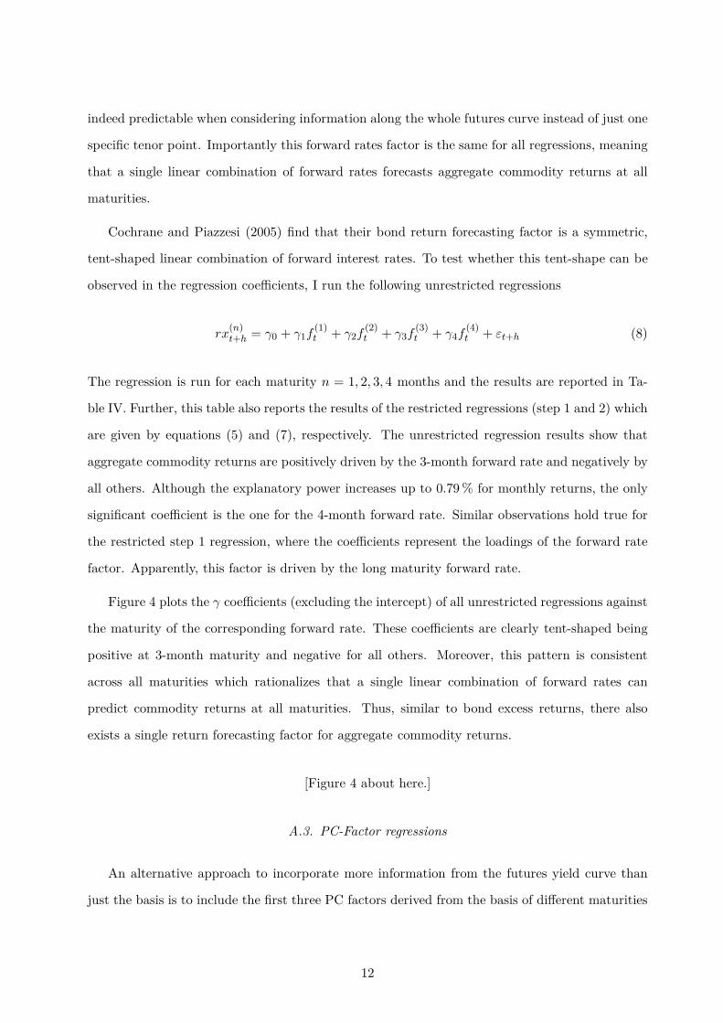
Cochrane and Piazzesi (2005) find that their bond return forecasting factor is a symmetric,
tent-shaped linear combination of forward interest rates. To test whether this tent-shape can be
observed in the regression coefficients, I run the following unrestricted regressions
rx(n)t+h = γ0 + γ1f
(1)t + γ2f
(2)t + γ3f
(3)t + γ4f
(4)t + εt+h (8)
The regression is run for each maturity n = 1, 2, 3, 4 months and the results are reported in Ta-
ble IV. Further, this table also reports the results of the restricted regressions (step 1 and 2) which
are given by equations (5) and (7), respectively. The unrestricted regression results show that
aggregate commodity returns are positively driven by the 3-month forward rate and negatively by
all others. Although the explanatory power increases up to 0.79 % for monthly returns, the only
significant coefficient is the one for the 4-month forward rate. Similar observations hold true for
the restricted step 1 regression, where the coefficients represent the loadings of the forward rate
factor. Apparently, this factor is driven by the long maturity forward rate.
Figure 4 plots the γ coefficients (excluding the intercept) of all unrestricted regressions against
the maturity of the corresponding forward rate. These coefficients are clearly tent-shaped being
positive at 3-month maturity and negative for all others. Moreover, this pattern is consistent
across all maturities which rationalizes that a single linear combination of forward rates can
predict commodity returns at all maturities. Thus, similar to bond excess returns, there also
exists a single return forecasting factor for aggregate commodity returns.
[Figure 4 about here.]
A.3. PC-Factor regressions
An alternative approach to incorporate more information from the futures yield curve than
just the basis is to include the first three PC factors derived from the basis of different maturities
12
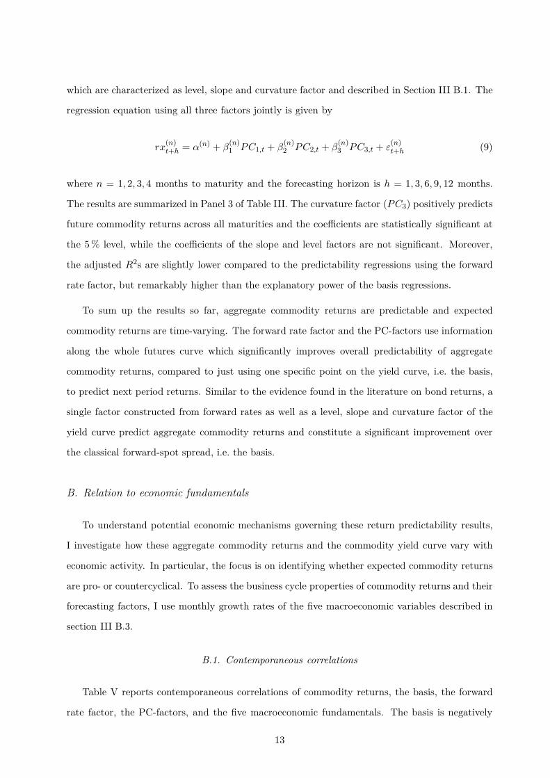
which are characterized as level, slope and curvature factor and described in Section III B.1. The
regression equation using all three factors jointly is given by
rx(n)t+h = α(n) + β
(n)1 PC1,t + β
(n)2 PC2,t + β
(n)3 PC3,t + ε
(n)t+h (9)
where n = 1, 2, 3, 4 months to maturity and the forecasting horizon is h = 1, 3, 6, 9, 12 months.
The results are summarized in Panel 3 of Table III. The curvature factor (PC3) positively predicts
future commodity returns across all maturities and the coefficients are statistically significant at
the 5 % level, while the coefficients of the slope and level factors are not significant. Moreover,
the adjusted R2s are slightly lower compared to the predictability regressions using the forward
rate factor, but remarkably higher than the explanatory power of the basis regressions.
To sum up the results so far, aggregate commodity returns are predictable and expected
commodity returns are time-varying. The forward rate factor and the PC-factors use information
along the whole futures curve which significantly improves overall predictability of aggregate
commodity returns, compared to just using one specific point on the yield curve, i.e. the basis,
to predict next period returns. Similar to the evidence found in the literature on bond returns, a
single factor constructed from forward rates as well as a level, slope and curvature factor of the
yield curve predict aggregate commodity returns and constitute a significant improvement over
the classical forward-spot spread, i.e. the basis.
B. Relation to economic fundamentals
To understand potential economic mechanisms governing these return predictability results,
I investigate how these aggregate commodity returns and the commodity yield curve vary with
economic activity. In particular, the focus is on identifying whether expected commodity returns
are pro- or countercyclical. To assess the business cycle properties of commodity returns and their
forecasting factors, I use monthly growth rates of the five macroeconomic variables described in
section III B.3.
B.1. Contemporaneous correlations
Table V reports contemporaneous correlations of commodity returns, the basis, the forward
rate factor, the PC-factors, and the five macroeconomic fundamentals. The basis is negatively
13
correlated with industrial production, export and import growth. On the other hand, the forward
rate factor and the curvature factor (PC3) are both positively correlated with all five economic fun-
damentals. The idea is that forecasted commodity returns should inherit the cyclical behaviour of
their forecasting factors. For example, the basis negatively predicts aggregate commodity returns
and it is negatively correlated with economic fundamentals, which would suggest a procyclical
behaviour of expected commodity returns. In times of economic growth, the commodity basis will
be low or even negative (backwardation) and thus predict positive returns on commodity futures.
The intuition is easier when looking at the other two dominant return forecasting factors. The
forward rate as well as the curvature factor positively predict aggregate commodity returns and
are positively correlated with economic fundamentals, hence, expected returns should be procycli-
cal. Nevertheless, these contemporaneous correlations and the subsequent deductions are just a
first indication that expected returns on an aggregate commodity portfolio might be procyclical.
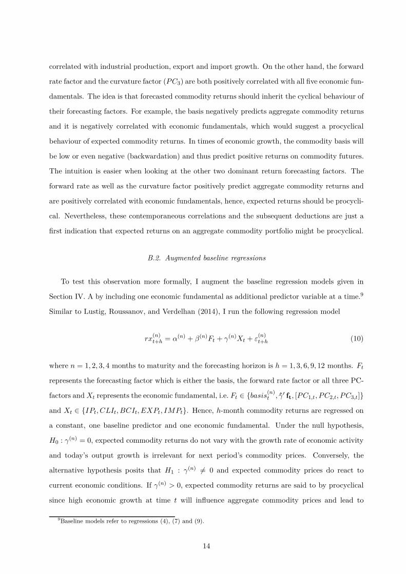
B.2. Augmented baseline regressions
To test this observation more formally, I augment the baseline regression models given in
Section IV. A by including one economic fundamental as additional predictor variable at a time.9
Similar to Lustig, Roussanov, and Verdelhan (2014), I run the following regression model
rx(n)t+h = α(n) + β(n)Ft + γ(n)Xt + ε
(n)t+h (10)
where n = 1, 2, 3, 4 months to maturity and the forecasting horizon is h = 1, 3, 6, 9, 12 months. Ft
represents the forecasting factor which is either the basis, the forward rate factor or all three PC-
factors and Xt represents the economic fundamental, i.e. Ft ∈ {basis(n)t , γ̂′ ft, [PC1,t, PC2,t, PC3,t]}
and Xt ∈ {IPt, CLIt, BCIt, EXPt, IMPt}. Hence, h-month commodity returns are regressed on
a constant, one baseline predictor and one economic fundamental. Under the null hypothesis,
H0 : γ(n) = 0, expected commodity returns do not vary with the growth rate of economic activity
and today’s output growth is irrelevant for next period’s commodity prices. Conversely, the
alternative hypothesis posits that H1 : γ(n) 6= 0 and expected commodity prices do react to
current economic conditions. If γ(n) > 0, expected commodity returns are said to by procyclical
since high economic growth at time t will influence aggregate commodity prices and lead to
9Baseline models refer to regressions (4), (7) and (9).
14
positive expected returns h-month ahead. Alternatively, γ(n) < 0 suggests that expected returns
of an aggregate commodity portfolio are countercyclical.
Table VI summarizes the results of these macroeconomic predictability regressions. The
columns labelled “Model” refer to one of the three baseline factors and the rows specify the
corresponding economic fundamental. For each combination of forecasting factors, the table re-
ports results for maturities, n, of 1 and 4 months, as well as a forecasting horizon, h, of 1 (Panel A)
and 12 months (Panel B).10 First, economic fundamentals positively predict aggregate commodity
returns. Their predictive power holds across maturities and it is strongest for short forecasting
horizons, i.e. at a monthly horizon all γ(n) coefficients are highly significant at a 5 % level. On
average the explanatory power given by the adjusted R2 slightly increases with the remaining
time to maturity, n, implying that prices of commodity futures with longer time to maturity
are more sensitive to current economic conditions. Second, using the forward rate factor or the
PC-factors jointly with economic fundamentals raises overall predictability as measured by the
R2adj to 7 %. In terms of baseline factors, the weakest one is the basis which is never significant
and hardly adds any predictive power while the forward rate factor is the most dominant baseline
predictor and its marginal significance is not reduced compared to the baseline model. Regarding
the economic fundamentals, the monthly changes of the composite leading indicator as well as the
business confidence index have the strongest predictive power and their coefficients are significant
across all different specifications.
Economically, these results imply that expected aggregate commodity returns are positive,
when industrial production or global trade increases. For example, a 1 % increase in total OECD
industrial production predicts positive returns of over 70 basis points for the next month for an
aggregate commodity portfolio. Note that these returns are already in excess of the risk-free rate
and without leverage, since futures positions are fully collateralized. Similarly, a monthly growth
rate of 1 % in global exports or imports of goods and services corresponds to expected monthly
commodity returns of nearly 15 basis points. Further, commodity prices are expected to increase
when managers are more confident about future business developments or when different economic
variables, aggregated to a composite leading indicator, point at higher economic activity.
From these findings I conclude that expected returns of an aggregate commodity portfolio are
procyclical. In economic terms, this means that an increase in global economic activity raises
10Further results are available on request.
15
the demand for commodities as production inputs. Consequently, a higher commodity demand
pushes up commodity spot prices and reduces existing inventories since commodity supply is
rather inelastic and it is difficult to adjust production immediately. Moreover, higher economic
activity raises commodity spot prices more than futures prices due to the fact that production
inputs are needed immediately and not n months in the future. Hence, the commodity yield curve
gets inverted (backwardation) and expected returns are high. Conversely, in times of economic
downturn the demand for commodities as production inputs decreases which in turn leads to a
fall in spot prices and a rise in inventory levels. This decrease in commodity demand, due to a
decline in industrial production, affects spot prices more strongly than futures prices which results
in an upward sloping commodity yield curve (contango). Hence, aggregate commodity returns
are expected to be low. Overall, these results show that expected returns on commodity futures
move in sync with economic activity and can thus be classified as procyclical.
C. Out-of-sample return predictability
Previous results and observations rely on in-sample return predictability analysis. They doc-
ument that commodity returns are predictable and some promising predictor variables have been
identified, such as the forward rate factor or different economic fundamentals. However, to fur-
ther use these results for investment purposes, one needs a proper out-of-sample backtest of these
models and variables. That is, I use the first 10 years of data, i.e. January 1975 to December
1984, to calibrate the model and estimate the regression parameters. Using these coefficient es-
timates together with the December 1984 observation of the predictor variables, I obtain the
first out-of-sample return forecast for January 1985 (forecasting horizon of 1 month). After one
month, I re-estimate the model with extended data from January 1975 to January 1985, to predict
the out-of-sample return for the next month. This iterative procedure is repeated every month
over an expanding data window to get consistent out-of-sample forecasts that are free from any
forward-looking bias. Hence, out-of-sample forecasts can be evaluated from January 1985 to
August 2015.
In order to investigate the reliability of the baseline predictors as well as the economic fun-
damentals for possible investment purposes, I estimate out-of-sample commodity return forecasts
using regression equation (10) for n = 1, 2, 3, 4 months to maturity and a forecasting horizon of
16
h = 1, 3, 6, 9, 12 months. Note that the forward rate factor and the PC-factors are re-estimated
each month to avoid any in-sample overfitting. To evaluate these out-of-sample return forecasts I
use the Campbell and Thompson (2008) R2OOS statistic, which compares the forecast accuracy of a
given predictive (regression) model relative to the historical average return forecast. In particular,
a positive R2OOS indicates that the model-based return forecast has a lower mean squared forecast
error than the historical average forecast, i.e. it is more accurate, and vice-versa if the R2OOS is
negative. To test whether the model based return forecasting improvement is also statistically
significant, I rely on the Clark and West (2007) MSFE-adjusted test statistic.11
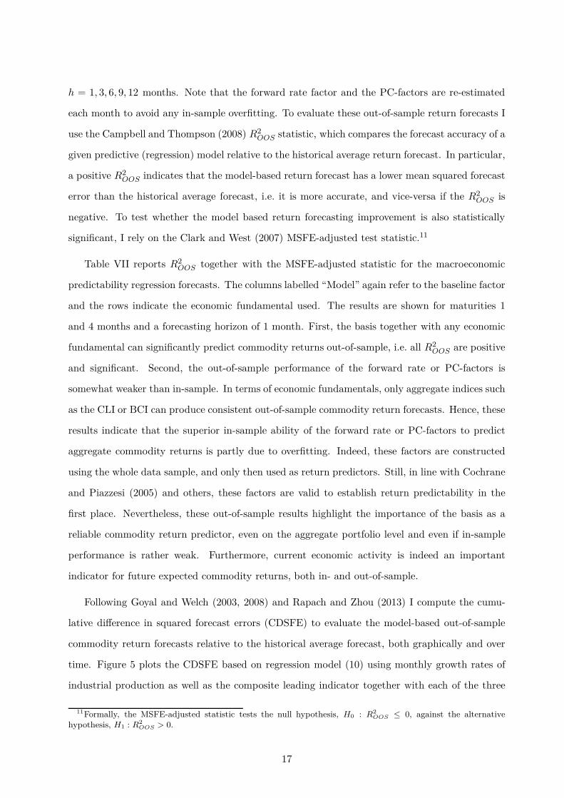
Table VII reports R2OOS together with the MSFE-adjusted statistic for the macroeconomic
predictability regression forecasts. The columns labelled “Model” again refer to the baseline factor
and the rows indicate the economic fundamental used. The results are shown for maturities 1
and 4 months and a forecasting horizon of 1 month. First, the basis together with any economic
fundamental can significantly predict commodity returns out-of-sample, i.e. all R2OOS are positive
and significant. Second, the out-of-sample performance of the forward rate or PC-factors is
somewhat weaker than in-sample. In terms of economic fundamentals, only aggregate indices such
as the CLI or BCI can produce consistent out-of-sample commodity return forecasts. Hence, these
results indicate that the superior in-sample ability of the forward rate or PC-factors to predict
aggregate commodity returns is partly due to overfitting. Indeed, these factors are constructed
using the whole data sample, and only then used as return predictors. Still, in line with Cochrane
and Piazzesi (2005) and others, these factors are valid to establish return predictability in the
first place. Nevertheless, these out-of-sample results highlight the importance of the basis as a
reliable commodity return predictor, even on the aggregate portfolio level and even if in-sample
performance is rather weak. Furthermore, current economic activity is indeed an important
indicator for future expected commodity returns, both in- and out-of-sample.
Following Goyal and Welch (2003, 2008) and Rapach and Zhou (2013) I compute the cumu-
lative difference in squared forecast errors (CDSFE) to evaluate the model-based out-of-sample
commodity return forecasts relative to the historical average forecast, both graphically and over
time. Figure 5 plots the CDSFE based on regression model (10) using monthly growth rates of
industrial production as well as the composite leading indicator together with each of the three
11Formally, the MSFE-adjusted statistic tests the null hypothesis, H0 : R2OOS ≤ 0, against the alternative
hypothesis, H1 : R2OOS > 0.
17
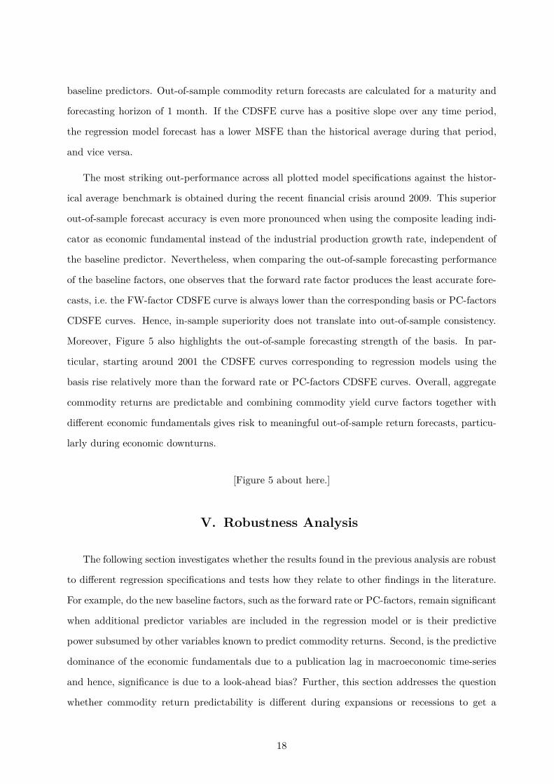
baseline predictors. Out-of-sample commodity return forecasts are calculated for a maturity and
forecasting horizon of 1 month. If the CDSFE curve has a positive slope over any time period,
the regression model forecast has a lower MSFE than the historical average during that period,
and vice versa.
The most striking out-performance across all plotted model specifications against the histor-
ical average benchmark is obtained during the recent financial crisis around 2009. This superior
out-of-sample forecast accuracy is even more pronounced when using the composite leading indi-
cator as economic fundamental instead of the industrial production growth rate, independent of
the baseline predictor. Nevertheless, when comparing the out-of-sample forecasting performance
of the baseline factors, one observes that the forward rate factor produces the least accurate fore-
casts, i.e. the FW-factor CDSFE curve is always lower than the corresponding basis or PC-factors
CDSFE curves. Hence, in-sample superiority does not translate into out-of-sample consistency.
Moreover, Figure 5 also highlights the out-of-sample forecasting strength of the basis. In par-
ticular, starting around 2001 the CDSFE curves corresponding to regression models using the
basis rise relatively more than the forward rate or PC-factors CDSFE curves. Overall, aggregate
commodity returns are predictable and combining commodity yield curve factors together with
different economic fundamentals gives risk to meaningful out-of-sample return forecasts, particu-
larly during economic downturns.
[Figure 5 about here.]
V. Robustness Analysis
The following section investigates whether the results found in the previous analysis are robust
to different regression specifications and tests how they relate to other findings in the literature.
For example, do the new baseline factors, such as the forward rate or PC-factors, remain significant
when additional predictor variables are included in the regression model or is their predictive
power subsumed by other variables known to predict commodity returns. Second, is the predictive
dominance of the economic fundamentals due to a publication lag in macroeconomic time-series
and hence, significance is due to a look-ahead bias? Further, this section addresses the question
whether commodity return predictability is different during expansions or recessions to get a
18
better understanding of the cyclicality of expected commodity returns. Last and most relevant
for investors is the analysis on predicting commodity index returns.
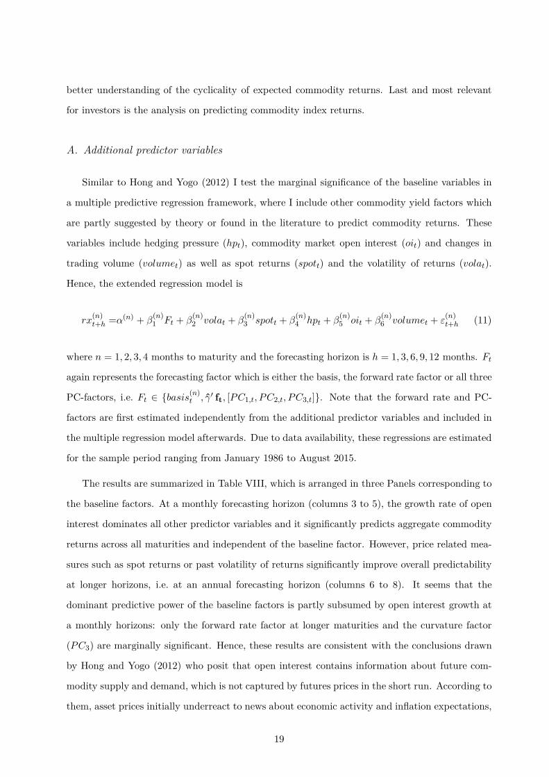
A. Additional predictor variables
Similar to Hong and Yogo (2012) I test the marginal significance of the baseline variables in
a multiple predictive regression framework, where I include other commodity yield factors which
are partly suggested by theory or found in the literature to predict commodity returns. These
variables include hedging pressure (hpt), commodity market open interest (oit) and changes in
trading volume (volumet) as well as spot returns (spott) and the volatility of returns (volat).
Hence, the extended regression model is
rx(n)t+h =α(n) + β
(n)1 Ft + β
(n)2 volat + β
(n)3 spott + β
(n)4 hpt + β
(n)5 oit + β
(n)6 volumet + ε
(n)t+h (11)
where n = 1, 2, 3, 4 months to maturity and the forecasting horizon is h = 1, 3, 6, 9, 12 months. Ft
again represents the forecasting factor which is either the basis, the forward rate factor or all three
PC-factors, i.e. Ft ∈ {basis(n)t , γ̂′ ft, [PC1,t, PC2,t, PC3,t]}. Note that the forward rate and PC-
factors are first estimated independently from the additional predictor variables and included in
the multiple regression model afterwards. Due to data availability, these regressions are estimated
for the sample period ranging from January 1986 to August 2015.
The results are summarized in Table VIII, which is arranged in three Panels corresponding to
the baseline factors. At a monthly forecasting horizon (columns 3 to 5), the growth rate of open
interest dominates all other predictor variables and it significantly predicts aggregate commodity
returns across all maturities and independent of the baseline factor. However, price related mea-
sures such as spot returns or past volatility of returns significantly improve overall predictability
at longer horizons, i.e. at an annual forecasting horizon (columns 6 to 8). It seems that the
dominant predictive power of the baseline factors is partly subsumed by open interest growth at
a monthly horizons: only the forward rate factor at longer maturities and the curvature factor
(PC3) are marginally significant. Hence, these results are consistent with the conclusions drawn
by Hong and Yogo (2012) who posit that open interest contains information about future com-
modity supply and demand, which is not captured by futures prices in the short run. According to
them, asset prices initially underreact to news about economic activity and inflation expectations,
19
which is better captured by open interest, since prices adjust only after a few months. Further-
more, the hedging pressure is never significant neither at the monthly or annual horizon nor at
short or long maturities. Although the coefficients are positive (which is in line with the theory
of normal backwardation, i.e. net short positions by hedgers imply positive expected returns on
commodity futures), their predictive power is obviously subsumed by more dominant variables.
Thus, the theory of normal backwardation is less relevant for describing expected returns, at least
on the aggregate commodity market level. Nevertheless, the explanatory power of the extended
regression model is more than doubled with adjusted R2s of over 3 %, compared to the baseline
regression models.
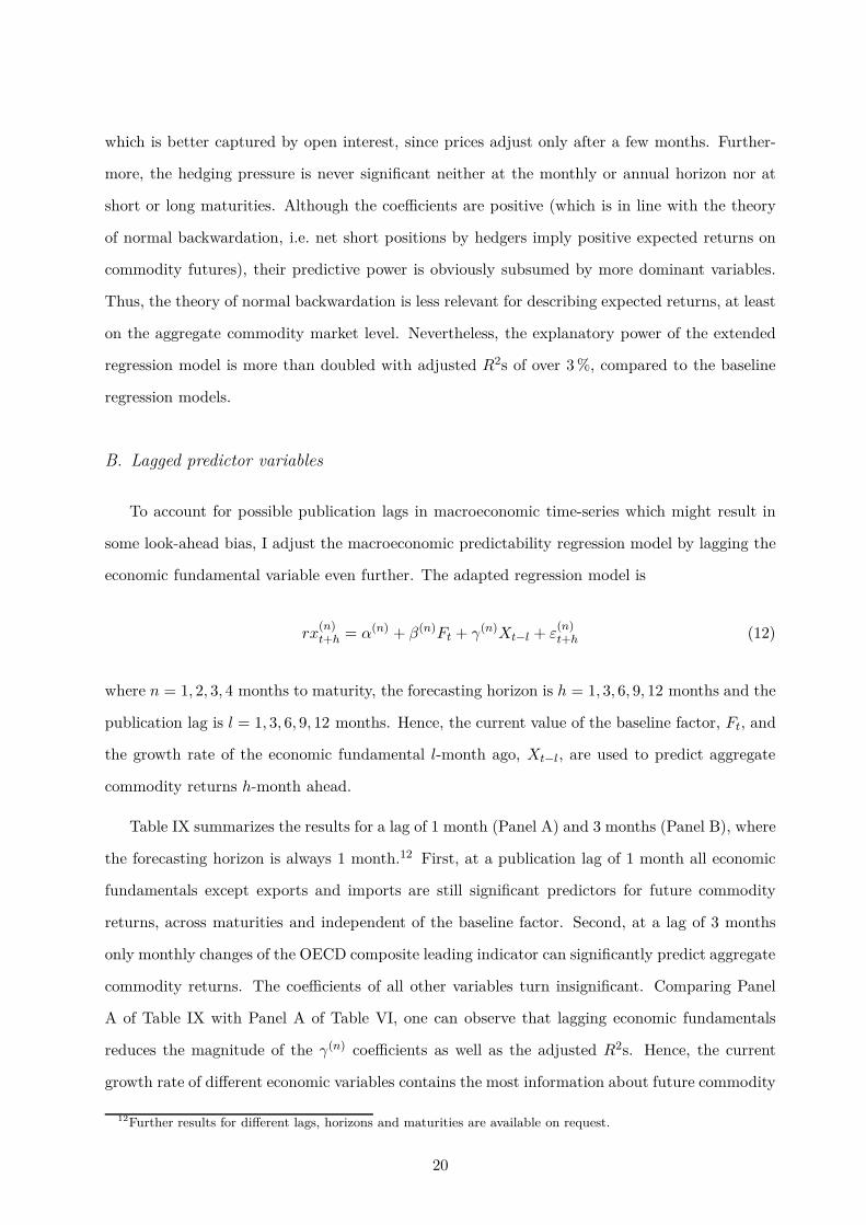
B. Lagged predictor variables
To account for possible publication lags in macroeconomic time-series which might result in
some look-ahead bias, I adjust the macroeconomic predictability regression model by lagging the
economic fundamental variable even further. The adapted regression model is
rx(n)t+h = α(n) + β(n)Ft + γ(n)Xt−l + ε
(n)t+h (12)
where n = 1, 2, 3, 4 months to maturity, the forecasting horizon is h = 1, 3, 6, 9, 12 months and the
publication lag is l = 1, 3, 6, 9, 12 months. Hence, the current value of the baseline factor, Ft, and
the growth rate of the economic fundamental l-month ago, Xt−l, are used to predict aggregate
commodity returns h-month ahead.
Table IX summarizes the results for a lag of 1 month (Panel A) and 3 months (Panel B), where
the forecasting horizon is always 1 month.12 First, at a publication lag of 1 month all economic
fundamentals except exports and imports are still significant predictors for future commodity
returns, across maturities and independent of the baseline factor. Second, at a lag of 3 months
only monthly changes of the OECD composite leading indicator can significantly predict aggregate
commodity returns. The coefficients of all other variables turn insignificant. Comparing Panel
A of Table IX with Panel A of Table VI, one can observe that lagging economic fundamentals
reduces the magnitude of the γ(n) coefficients as well as the adjusted R2s. Hence, the current
growth rate of different economic variables contains the most information about future commodity
12Further results for different lags, horizons and maturities are available on request.
20
prices. However, even with a publication lag of one month most results in terms of statistical
significance continue to hold, albeit with smaller economic magnitude. Moreover, the regression
coefficients of lagged economic fundamentals are all positive, implying that expected aggregate
commodity returns are procyclical.
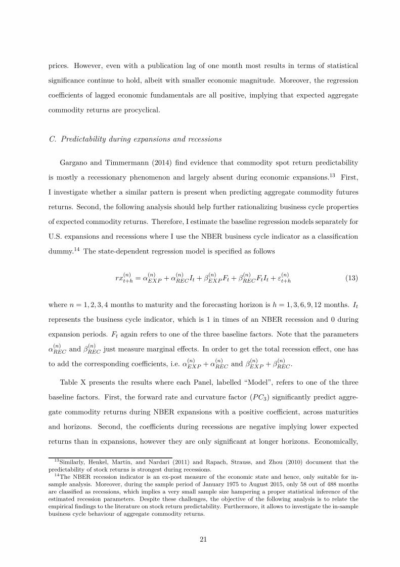
C. Predictability during expansions and recessions
Gargano and Timmermann (2014) find evidence that commodity spot return predictability
is mostly a recessionary phenomenon and largely absent during economic expansions.13 First,
I investigate whether a similar pattern is present when predicting aggregate commodity futures
returns. Second, the following analysis should help further rationalizing business cycle properties
of expected commodity returns. Therefore, I estimate the baseline regression models separately for
U.S. expansions and recessions where I use the NBER business cycle indicator as a classification
dummy.14 The state-dependent regression model is specified as follows
rx(n)t+h = α
(n)EXP + α
(n)RECIt + β
(n)EXP Ft + β
(n)RECFtIt + ε
(n)t+h (13)
where n = 1, 2, 3, 4 months to maturity and the forecasting horizon is h = 1, 3, 6, 9, 12 months. It
represents the business cycle indicator, which is 1 in times of an NBER recession and 0 during
expansion periods. Ft again refers to one of the three baseline factors. Note that the parameters
α(n)REC and β
(n)REC just measure marginal effects. In order to get the total recession effect, one has
to add the corresponding coefficients, i.e. α(n)EXP + α
(n)REC and β
(n)EXP + β
(n)REC .
Table X presents the results where each Panel, labelled “Model”, refers to one of the three
baseline factors. First, the forward rate and curvature factor (PC3) significantly predict aggre-
gate commodity returns during NBER expansions with a positive coefficient, across maturities
and horizons. Second, the coefficients during recessions are negative implying lower expected
returns than in expansions, however they are only significant at longer horizons. Economically,
13Similarly, Henkel, Martin, and Nardari (2011) and Rapach, Strauss, and Zhou (2010) document that thepredictability of stock returns is strongest during recessions.
14The NBER recession indicator is an ex-post measure of the economic state and hence, only suitable for in-sample analysis. Moreover, during the sample period of January 1975 to August 2015, only 58 out of 488 monthsare classified as recessions, which implies a very small sample size hampering a proper statistical inference of theestimated recession parameters. Despite these challenges, the objective of the following analysis is to relate theempirical findings to the literature on stock return predictability. Furthermore, it allows to investigate the in-samplebusiness cycle behaviour of aggregate commodity returns.
21

these results indicate that aggregate commodity returns are expected to be positive and high
during economic expansions, whereas they tend to be low or partly even negative during re-
cessions. Hence, expected commodity returns are clearly procyclical, increasing with economic
activity and decreasing during downturns, which is consistent with the evidence found when using
different economic fundamentals to predict returns. Third, it seems that aggregate commodity
return predictability is an expansionary phenomenon which is clearly in contrast to the findings
on stock return predictability. Of course the weak statistical significance of estimated recession
coefficients is partly due to the small sample size, however studies on the state-dependencies of
stock returns are prone to the same problem. Still, the results are different and I find that the
predictability of commodity returns is strongest during expansions and their business cycle be-
haviour is procyclical. Furthermore, the adjusted R2s of these state-dependent regressions are
significantly higher than the ones of the baseline regressions. Hence, the explanatory power of the
baseline factors seems to increase if we account for the economic state when predicting aggregate
commodity returns. Last, the coefficients of the basis are insignificant across all maturities and
horizons, implying that the basis cannot predict aggregate commodity returns even if we account
for state-dependencies. Thus, using information along the whole futures curve significantly im-
proves the in-sample predictive power and allows to analyze state-dependencies and the business
cycle behaviour of expected commodity returns.
D. Predicting commodity index returns
To test the relevance of these identified commodity return predictors for investors, I use the
baseline factors together with the economic fundamentals to predict returns on commodity indices.
That is, I estimate the macroeconomic predictability regression model given by equation (10), but
instead of forecasting returns on a constructed commodity portfolio I use monthly returns on the
SP-GSCI as well as the DJ-UBS commodity index. Note that these indices are not available for
different maturities, since they are always rolled over to the nearest contract.
Panel A of Table XI presents the results for predicting monthly SP-GSCI returns. First, the
aggregate commodity basis significantly predicts SP-GSCI returns. The coefficients are negative
which is in line with the expected roll yield, i.e. positive returns in a backwardated futures
market and negative returns when the commodity market is in contango. Interestingly, the
22
aggregate basis can predict expected returns on a commodity index but not on its own commodity
portfolio. Second, the coefficients of the forward rate and curvature (PC3) factor are all highly
significant, positive and their magnitude is remarkably higher than the corresponding coefficients
when predicting aggregate commodity returns (see Panel A of Table VI). This implies that the
information along the aggregate futures curves seems to be very relevant for commodity index
returns. Third, all economic fundamentals, except export growth, significantly predict monthly
returns on the SP-GSCI and their marginal effect is stronger than for aggregate commodity
returns (i.e. the γ coefficients in Table XI are twice the size of the γ(n) coefficients in Table VI).
Moreover, all coefficients are positive implying that commodity index returns are also procyclical
and increase with economic activity. Overall, the explanatory power, i.e. adjusted R2s, of these
macroeconomic predictability regressions is very similar when predicting aggregate commodity
returns or commodity index returns.
Panel B of Table XI reports results for predicting monthly returns on the DJ-UBS commodity
index. Due to data availability the sample period is shorter and starts in January 1991 to August
2015. Although the marginal effects of all baseline factors are insignificant, all economic funda-
mentals, expect export growth, are highly relevant for predicting returns on this index. Similarly,
their coefficients are positive and DJ-UBS commodity index returns are also procyclical. To sum
up, the macroeconomic predictive regression model also allows to forecast monthly returns of
tradable commodity indices.
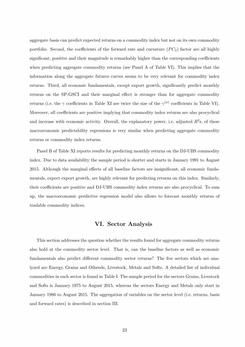
VI. Sector Analysis
This section addresses the question whether the results found for aggregate commodity returns
also hold at the commodity sector level. That is, can the baseline factors as well as economic
fundamentals also predict different commodity sector returns? The five sectors which are ana-
lyzed are Energy, Grains and Oilseeds, Livestock, Metals and Softs. A detailed list of individual
commodities in each sector is found in Table I. The sample period for the sectors Grains, Livestock
and Softs is January 1975 to August 2015, whereas the sectors Energy and Metals only start in
January 1986 to August 2015. The aggregation of variables on the sector level (i.e. returns, basis
and forward rates) is described in section III.
23
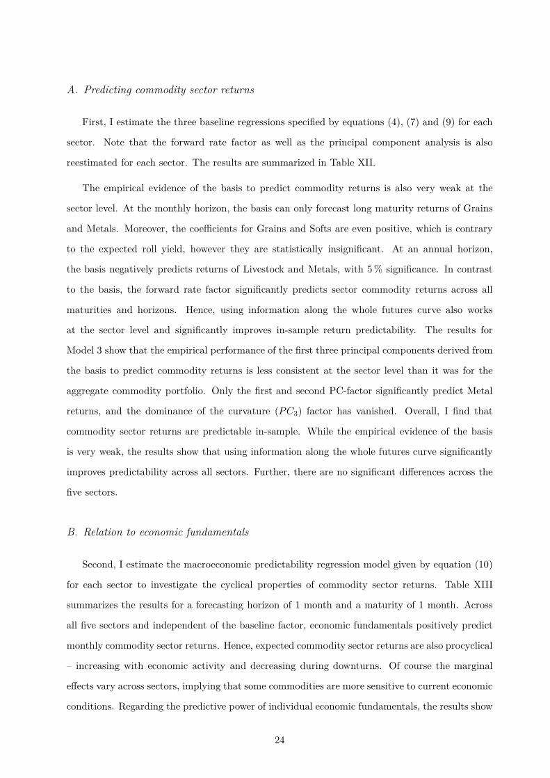
A. Predicting commodity sector returns
First, I estimate the three baseline regressions specified by equations (4), (7) and (9) for each
sector. Note that the forward rate factor as well as the principal component analysis is also
reestimated for each sector. The results are summarized in Table XII.
The empirical evidence of the basis to predict commodity returns is also very weak at the
sector level. At the monthly horizon, the basis can only forecast long maturity returns of Grains
and Metals. Moreover, the coefficients for Grains and Softs are even positive, which is contrary
to the expected roll yield, however they are statistically insignificant. At an annual horizon,
the basis negatively predicts returns of Livestock and Metals, with 5 % significance. In contrast
to the basis, the forward rate factor significantly predicts sector commodity returns across all
maturities and horizons. Hence, using information along the whole futures curve also works
at the sector level and significantly improves in-sample return predictability. The results for
Model 3 show that the empirical performance of the first three principal components derived from
the basis to predict commodity returns is less consistent at the sector level than it was for the
aggregate commodity portfolio. Only the first and second PC-factor significantly predict Metal
returns, and the dominance of the curvature (PC3) factor has vanished. Overall, I find that
commodity sector returns are predictable in-sample. While the empirical evidence of the basis
is very weak, the results show that using information along the whole futures curve significantly
improves predictability across all sectors. Further, there are no significant differences across the
five sectors.
B. Relation to economic fundamentals
Second, I estimate the macroeconomic predictability regression model given by equation (10)
for each sector to investigate the cyclical properties of commodity sector returns. Table XIII
summarizes the results for a forecasting horizon of 1 month and a maturity of 1 month. Across
all five sectors and independent of the baseline factor, economic fundamentals positively predict
monthly commodity sector returns. Hence, expected commodity sector returns are also procyclical
– increasing with economic activity and decreasing during downturns. Of course the marginal
effects vary across sectors, implying that some commodities are more sensitive to current economic
conditions. Regarding the predictive power of individual economic fundamentals, the results show
24

that monthly changes in the OECD composite leading indicator as well as the business confidence
index can significantly predict next month commodity returns of all sectors. While expected
returns of Energy and Metals are very sensitive to aggregate economic conditions, with CLI or
BCI coefficients of around 10, the corresponding coefficients of Grains and Softs are only around 5
and Livestock returns are the least sensitive with coefficients of only 2. Further, monthly growth
rates of global industrial production significantly predict commodity returns of the sectors Energy,
Metals and Softs, while growth rates of world exports and imports can predict returns of Energy
and Softs only. On the other hand, commodity returns of the sectors Grains and Livestock are
less affected by economic conditions.
These cross-sectional differences in sensitivities to economic conditions across commodity sec-
tors are consistent with the economic explanation for the cyclical properties of commodity returns.
That is, higher economic activity increases the demand for commodities as production inputs,
which in turn raises the spot price and reduces existing inventories. As a result, the commodity
yield curve gets inverted (backwardation) and expected returns on commodity futures are high
and positive. For this mechanism to work, the effect on commodity demand and the consequent
reaction of commodity spot prices and inventories is essential. I posit that this effect is much
stronger for commodities serving as production inputs for different industries. This is certainly
the case for Energy and Metals and to a certain degree also for Softs (which contains for ex-
ample Ethanol, Cotton or Sugar). On the other hand Grains and Oilseeds as well as Livestock
are not used as inputs for industrial production and hence the demand for these commodities is
rather inelastic to changes in production. Moreover, the demand for raw materials needed for
food production, which are basically Grains and Livestock, does not vary with economic activity
or the business cycle. Thus, these differences in commodity demand caused by time-variation
in industrial production translate to different marginal effects of economic fundamentals in the
predictability of commodity sector returns. While returns of Energy, Metals and Softs are very
sensitive to economic conditions with highly significant γ coefficients, returns of Grains and Live-
stock do not react to changes in economic activity.
Third, I estimate out-of-sample forecasts for commodity sector returns using again regression
equation (10). I use the first 10 years of data as an initial in-sample estimate, which is for
the sectors Grains, Livestock and Softs January 1975 to December 1984 and for Energy and
Metals it is January 1986 to December 1995. Then, out-of-sample forecasts are evaluated using
25
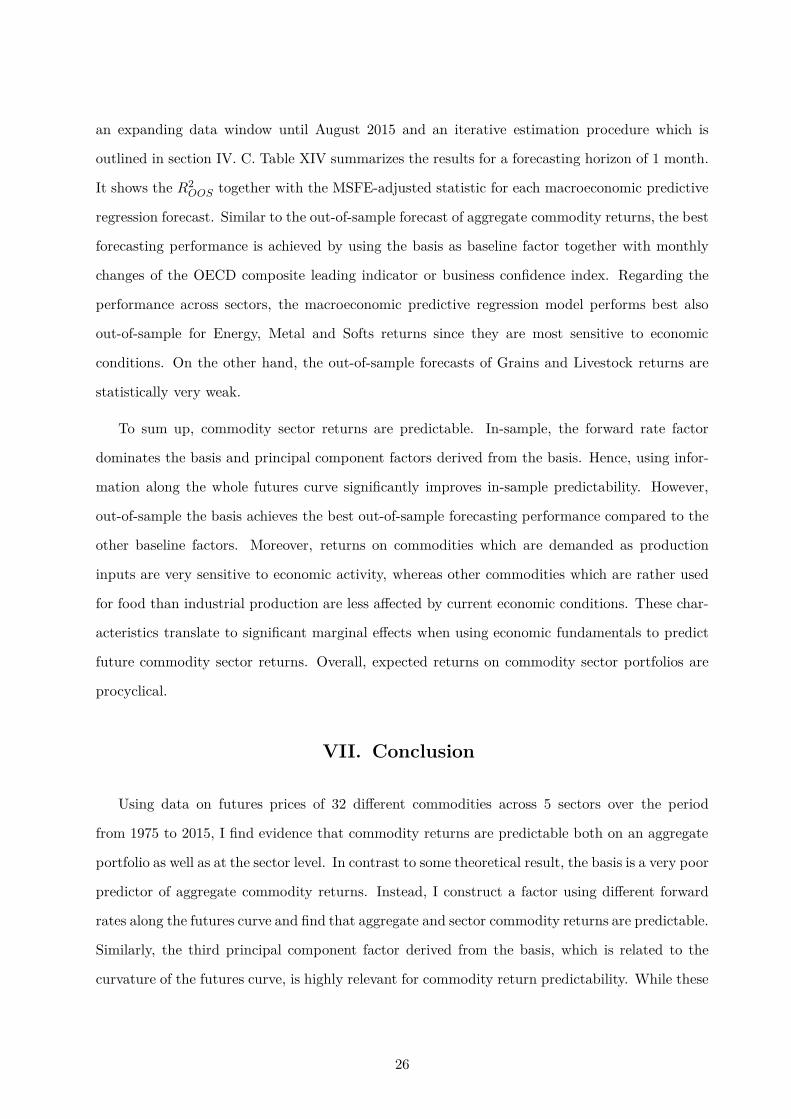
an expanding data window until August 2015 and an iterative estimation procedure which is
outlined in section IV. C. Table XIV summarizes the results for a forecasting horizon of 1 month.
It shows the R2OOS together with the MSFE-adjusted statistic for each macroeconomic predictive
regression forecast. Similar to the out-of-sample forecast of aggregate commodity returns, the best
forecasting performance is achieved by using the basis as baseline factor together with monthly
changes of the OECD composite leading indicator or business confidence index. Regarding the
performance across sectors, the macroeconomic predictive regression model performs best also
out-of-sample for Energy, Metal and Softs returns since they are most sensitive to economic
conditions. On the other hand, the out-of-sample forecasts of Grains and Livestock returns are
statistically very weak.
To sum up, commodity sector returns are predictable. In-sample, the forward rate factor
dominates the basis and principal component factors derived from the basis. Hence, using infor-
mation along the whole futures curve significantly improves in-sample predictability. However,
out-of-sample the basis achieves the best out-of-sample forecasting performance compared to the
other baseline factors. Moreover, returns on commodities which are demanded as production
inputs are very sensitive to economic activity, whereas other commodities which are rather used
for food than industrial production are less affected by current economic conditions. These char-
acteristics translate to significant marginal effects when using economic fundamentals to predict
future commodity sector returns. Overall, expected returns on commodity sector portfolios are
procyclical.
VII. Conclusion
Using data on futures prices of 32 different commodities across 5 sectors over the period
from 1975 to 2015, I find evidence that commodity returns are predictable both on an aggregate
portfolio as well as at the sector level. In contrast to some theoretical result, the basis is a very poor
predictor of aggregate commodity returns. Instead, I construct a factor using different forward
rates along the futures curve and find that aggregate and sector commodity returns are predictable.
Similarly, the third principal component factor derived from the basis, which is related to the
curvature of the futures curve, is highly relevant for commodity return predictability. While these
26

factors derived from the whole futures curve significantly improve in-sample predictability, the
basis achieves the best out-of-sample forecasting performance.
Second, I find evidence that expected aggregate commodity returns are procyclical and that
the time-variation in the commodity yield curve is strongly linked to the business cycle. Eco-
nomic fundamentals, such as industrial production or global trade, positively predict aggregate
and sector commodity returns. Using economic fundamentals jointly with these yield curve factors
significantly raises overall predictability in- and out-of-sample. I argue that higher economic ac-
tivity increases the demand for commodities as input factors, which in turn raises commodity spot
prices and lowers inventories. As a result, the commodity yield curve gets inverted (backwarda-
tion) and expected returns on commodity futures are high. Results on sector return predictability
show that commodities which are demanded as production inputs, such as Energy and Metals,
are very sensitive to changes in economic activity, whereas other commodities which are rather
used for food than industrial production are less affected by current economic conditions. These
characteristics translate to cross-sectional differences in marginal effects when using economic
fundamentals to predict future commodity sector returns.
27
References
Bailey, W., and K.C. Chan, 1993, Macroeconomic influences and the variability of the commodity futures
basis, Journal of Finance 48, 555–573.
Bessembinder, H., 1992, Systematic risk, hedging pressure, and risk premiums in futures markets, Review
of Financial Studies 5, 637–667.
Brennan, M.J., 1958, The supply of storage, The American Economic Review 48, 50–72.
Campbell, J.Y., and S.B. Thompson, 2008, Predicting excess stock returns out of sample: can anything
beat the historical average?, Review of Financial Studies 21, 1509–1531.
Chang, E.C., 1985, Returns to speculators and the theory of normal backwardation, Journal of Finance
40, 193–208.
Clark, T.E., and K.D. West, 2007, Approximately normal tests for equal predictive accuracy in nested
models, Journal of Econometrics 138, 291–311.
Cochrane, J.H., and M. Piazzesi, 2005, Bond risk premia, The American Economic Review 95, 138–160.
Cootner, P.H., 1960, Returns to speculators: Telser versus Keynes, Journal of Political Economy 68,
396–404.
de Roon, F.A., T.E. Nijman, and C. Veld, 2000, Hedging pressure effects in futures markets, Journal of
Finance 55, 1437–1456.
Erb, C.B., and C.R. Harvey, 2006, The strategic and tactical value of commodity futures, Financial
Analysts Journal 62, 69–97.
Fama, E.F., and K.R. French, 1987, Commodity futures prices: some evidence on forecast power, premiums,
and the theory of storage, Journal of Business 60, 55–73.
Fuertes, A.M., J. Miffre, and G. Rallis, 2010, Tactical allocation in commodity futures markets: combining
momentum and term structure signals, Journal of Banking & Finance 34, 2530–2548.
Gargano, A., and A. Timmermann, 2014, Forecasting commodity price indexes using macroeconomic and
financial predictors, International Journal of Forecasting 30, 825–843.
Gorton, G.B., F. Hayashi, and K.G. Rouwenhorst, 2012, The fundamentals of commodity futures returns,
Review of Finance 17, 35–105.
Goyal, A., and I. Welch, 2003, Predicting the equity premium with dividend ratios, Management Science
49, 639–654.
28
Goyal, A., and I. Welch, 2008, A comprehensive look at the empirical performance of equity premium
prediction, Review of Financial Studies 21, 1455–1508.
Henkel, S.J., J.S. Martin, and F. Nardari, 2011, Time-varying short-horizon predictability, Journal of
Financial Economics 99, 560–580.
Hicks, J.R., 1939, Value and capital. (Oxford: Clarendon Press).
Hong, H., and M. Yogo, 2012, What does futures market interest tell us about the macroeconomy and
asset prices?, Journal of Financial Economics 105, 473–490.
Kaldor, N., 1939, Speculation and economic stability, The Review of Economic Studies 7, 1–27.
Keynes, J.M., 1930, A treatise on money. (London Macmillan).
Lustig, H., N. Roussanov, and A. Verdelhan, 2014, Countercyclical currency risk premia, Journal of Fi-
nancial Economics 111, 527–553.
Newey, W.K., and K.D. West, 1987, A simple, positive semi-definite, heteroskedasticity and autocorrelation
consistent covariance matrix, Econometrica 55, 703–708.
Rapach, D.E, J.K. Strauss, and G. Zhou, 2010, Out-of-sample equity premium prediction: combination
forecasts and links to the real economy, Review of Financial Studies 23, 821–862.
Rapach, D.E., and G. Zhou, 2013, Forecasting stock returns, in Handbook of Economic Forecasting (Else-
vier, Amsterdam ).
Szymanowska, M., F. de Roon, T. Nijman, and R. van den Goorbergh, 2014, An anatomy of commodity
futures risk premia, Journal of Finance 69, 453–482.
Working, H., 1933, Price relations between July and September wheat futures at Chicago since 1885, Wheat
Studies of the Food Research Institute 9, 187–238.
Yang, F., 2013, Investment shocks and the commodity basis spread, Journal of Financial Economics 110,
164–184.
29
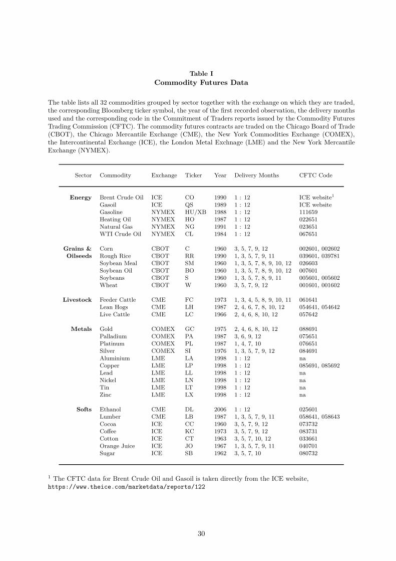
Table I
Commodity Futures Data
The table lists all 32 commodities grouped by sector together with the exchange on which they are traded,the corresponding Bloomberg ticker symbol, the year of the first recorded observation, the delivery monthsused and the corresponding code in the Commitment of Traders reports issued by the Commodity FuturesTrading Commission (CFTC). The commodity futures contracts are traded on the Chicago Board of Trade(CBOT), the Chicago Mercantile Exchange (CME), the New York Commodities Exchange (COMEX),the Intercontinental Exchange (ICE), the London Metal Exchnage (LME) and the New York MercantileExchange (NYMEX).
Sector Commodity Exchange Ticker Year Delivery Months CFTC Code
Energy Brent Crude Oil ICE CO 1990 1 : 12 ICE website1
Gasoil ICE QS 1989 1 : 12 ICE websiteGasoline NYMEX HU/XB 1988 1 : 12 111659Heating Oil NYMEX HO 1987 1 : 12 022651Natural Gas NYMEX NG 1991 1 : 12 023651WTI Crude Oil NYMEX CL 1984 1 : 12 067651
Grains & Corn CBOT C 1960 3, 5, 7, 9, 12 002601, 002602Oilseeds Rough Rice CBOT RR 1990 1, 3, 5, 7, 9, 11 039601, 039781
Soybean Meal CBOT SM 1960 1, 3, 5, 7, 8, 9, 10, 12 026603Soybean Oil CBOT BO 1960 1, 3, 5, 7, 8, 9, 10, 12 007601Soybeans CBOT S 1960 1, 3, 5, 7, 8, 9, 11 005601, 005602Wheat CBOT W 1960 3, 5, 7, 9, 12 001601, 001602
Livestock Feeder Cattle CME FC 1973 1, 3, 4, 5, 8, 9, 10, 11 061641Lean Hogs CME LH 1987 2, 4, 6, 7, 8, 10, 12 054641, 054642Live Cattle CME LC 1966 2, 4, 6, 8, 10, 12 057642
Metals Gold COMEX GC 1975 2, 4, 6, 8, 10, 12 088691Palladium COMEX PA 1987 3, 6, 9, 12 075651Platinum COMEX PL 1987 1, 4, 7, 10 076651Silver COMEX SI 1976 1, 3, 5, 7, 9, 12 084691Aluminium LME LA 1998 1 : 12 naCopper LME LP 1998 1 : 12 085691, 085692Lead LME LL 1998 1 : 12 naNickel LME LN 1998 1 : 12 naTin LME LT 1998 1 : 12 naZinc LME LX 1998 1 : 12 na
Softs Ethanol CME DL 2006 1 : 12 025601Lumber CME LB 1987 1, 3, 5, 7, 9, 11 058641, 058643Cocoa ICE CC 1960 3, 5, 7, 9, 12 073732Coffee ICE KC 1973 3, 5, 7, 9, 12 083731Cotton ICE CT 1963 3, 5, 7, 10, 12 033661Orange Juice ICE JO 1967 1, 3, 5, 7, 9, 11 040701Sugar ICE SB 1962 3, 5, 7, 10 080732
1 The CFTC data for Brent Crude Oil and Gasoil is taken directly from the ICE website,https://www.theice.com/marketdata/reports/122
30
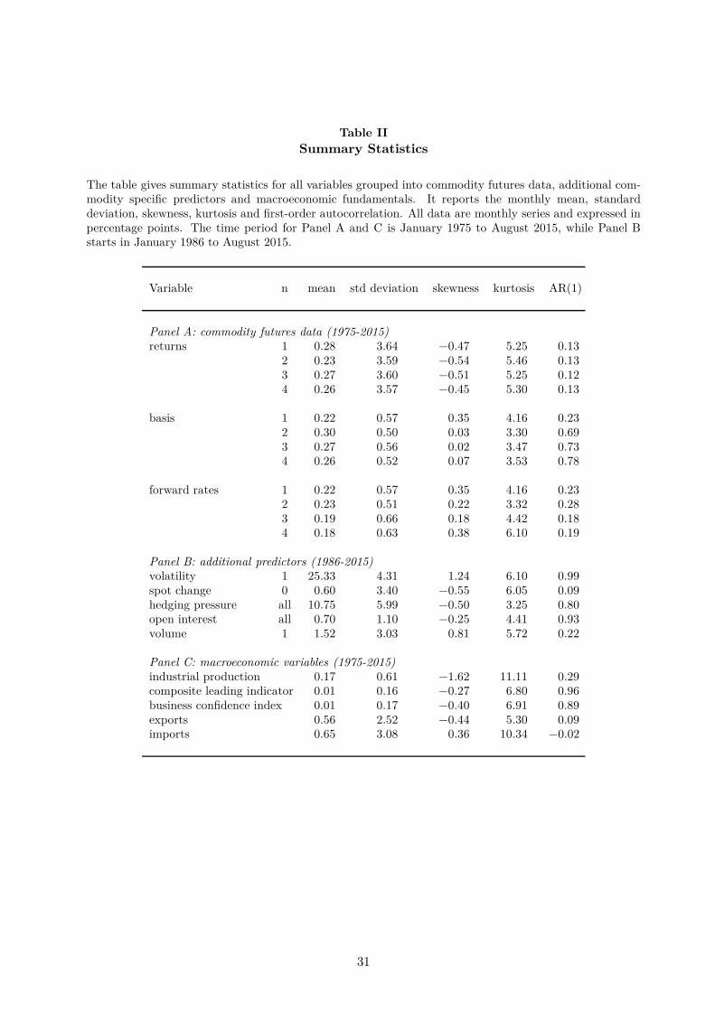
Table II
Summary Statistics
The table gives summary statistics for all variables grouped into commodity futures data, additional com-modity specific predictors and macroeconomic fundamentals. It reports the monthly mean, standarddeviation, skewness, kurtosis and first-order autocorrelation. All data are monthly series and expressed inpercentage points. The time period for Panel A and C is January 1975 to August 2015, while Panel Bstarts in January 1986 to August 2015.
Variable n mean std deviation skewness kurtosis AR(1)
Panel A: commodity futures data (1975-2015)returns 1 0.28 3.64 −0.47 5.25 0.13
2 0.23 3.59 −0.54 5.46 0.133 0.27 3.60 −0.51 5.25 0.124 0.26 3.57 −0.45 5.30 0.13
basis 1 0.22 0.57 0.35 4.16 0.232 0.30 0.50 0.03 3.30 0.693 0.27 0.56 0.02 3.47 0.734 0.26 0.52 0.07 3.53 0.78
forward rates 1 0.22 0.57 0.35 4.16 0.232 0.23 0.51 0.22 3.32 0.283 0.19 0.66 0.18 4.42 0.184 0.18 0.63 0.38 6.10 0.19
Panel B: additional predictors (1986-2015)volatility 1 25.33 4.31 1.24 6.10 0.99spot change 0 0.60 3.40 −0.55 6.05 0.09hedging pressure all 10.75 5.99 −0.50 3.25 0.80open interest all 0.70 1.10 −0.25 4.41 0.93volume 1 1.52 3.03 0.81 5.72 0.22
Panel C: macroeconomic variables (1975-2015)industrial production 0.17 0.61 −1.62 11.11 0.29composite leading indicator 0.01 0.16 −0.27 6.80 0.96business confidence index 0.01 0.17 −0.40 6.91 0.89exports 0.56 2.52 −0.44 5.30 0.09imports 0.65 3.08 0.36 10.34 −0.02
31
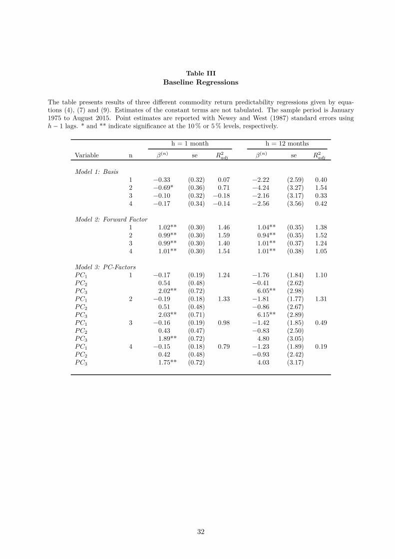
Table III
Baseline Regressions
The table presents results of three different commodity return predictability regressions given by equa-tions (4), (7) and (9). Estimates of the constant terms are not tabulated. The sample period is January1975 to August 2015. Point estimates are reported with Newey and West (1987) standard errors usingh − 1 lags. * and ** indicate significance at the 10 % or 5 % levels, respectively.
h = 1 month h = 12 months
Variable n β(n) se R2adj β(n) se R2
adj
Model 1: Basis1 −0.33 (0.32) 0.07 −2.22 (2.59) 0.402 −0.69* (0.36) 0.71 −4.24 (3.27) 1.543 −0.10 (0.32) −0.18 −2.16 (3.17) 0.334 −0.17 (0.34) −0.14 −2.56 (3.56) 0.42
Model 2: Forward Factor1 1.02** (0.30) 1.46 1.04** (0.35) 1.382 0.99** (0.30) 1.59 0.94** (0.35) 1.523 0.99** (0.30) 1.40 1.01** (0.37) 1.244 1.01** (0.30) 1.54 1.01** (0.38) 1.05
Model 3: PC-FactorsP C1 1 −0.17 (0.19) 1.24 −1.76 (1.84) 1.10P C2 0.54 (0.48) −0.41 (2.62)P C3 2.02** (0.72) 6.05** (2.98)P C1 2 −0.19 (0.18) 1.33 −1.81 (1.77) 1.31P C2 0.51 (0.48) −0.86 (2.67)P C3 2.03** (0.71) 6.15** (2.89)P C1 3 −0.16 (0.19) 0.98 −1.42 (1.85) 0.49P C2 0.43 (0.47) −0.83 (2.50)P C3 1.89** (0.72) 4.80 (3.05)P C1 4 −0.15 (0.18) 0.79 −1.23 (1.89) 0.19P C2 0.42 (0.48) −0.93 (2.42)P C3 1.75** (0.72) 4.03 (3.17)
32
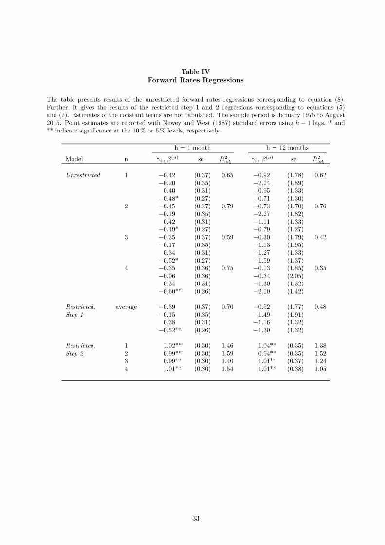
Table IV
Forward Rates Regressions
The table presents results of the unrestricted forward rates regressions corresponding to equation (8).Further, it gives the results of the restricted step 1 and 2 regressions corresponding to equations (5)and (7). Estimates of the constant terms are not tabulated. The sample period is January 1975 to August2015. Point estimates are reported with Newey and West (1987) standard errors using h − 1 lags. * and** indicate significance at the 10 % or 5 % levels, respectively.
h = 1 month h = 12 months
Model n γi , β(n) se R2adj γi , β(n) se R2
adj
Unrestricted 1 −0.42 (0.37) 0.65 −0.92 (1.78) 0.62−0.20 (0.35) −2.24 (1.89)
0.40 (0.31) −0.95 (1.33)−0.48* (0.27) −0.71 (1.30)
2 −0.45 (0.37) 0.79 −0.73 (1.70) 0.76−0.19 (0.35) −2.27 (1.82)
0.42 (0.31) −1.11 (1.33)−0.49* (0.27) −0.79 (1.27)
3 −0.35 (0.37) 0.59 −0.30 (1.79) 0.42−0.17 (0.35) −1.13 (1.95)
0.34 (0.31) −1.27 (1.33)−0.52* (0.27) −1.59 (1.37)
4 −0.35 (0.36) 0.75 −0.13 (1.85) 0.35−0.06 (0.36) −0.34 (2.05)
0.34 (0.31) −1.30 (1.32)−0.60** (0.26) −2.10 (1.42)
Restricted, average −0.39 (0.37) 0.70 −0.52 (1.77) 0.48Step 1 −0.15 (0.35) −1.49 (1.91)
0.38 (0.31) −1.16 (1.32)−0.52** (0.26) −1.30 (1.32)
Restricted, 1 1.02** (0.30) 1.46 1.04** (0.35) 1.38Step 2 2 0.99** (0.30) 1.59 0.94** (0.35) 1.52
3 0.99** (0.30) 1.40 1.01** (0.37) 1.244 1.01** (0.30) 1.54 1.01** (0.38) 1.05
33
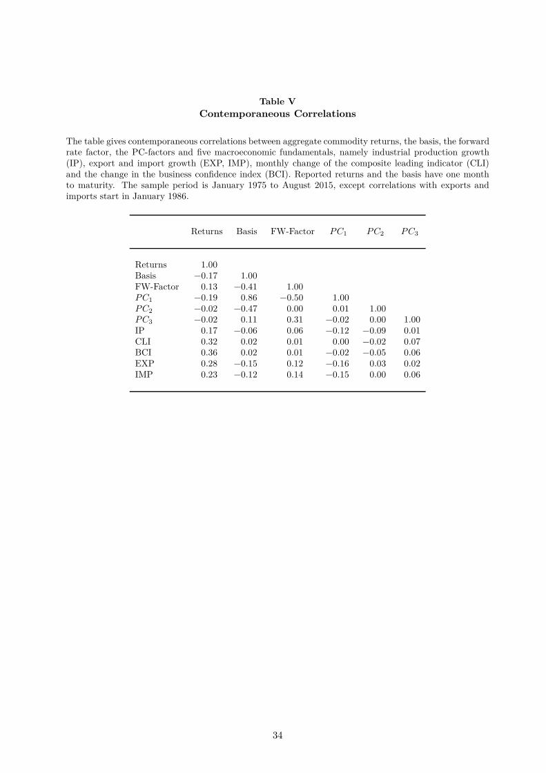
Table V
Contemporaneous Correlations
The table gives contemporaneous correlations between aggregate commodity returns, the basis, the forwardrate factor, the PC-factors and five macroeconomic fundamentals, namely industrial production growth(IP), export and import growth (EXP, IMP), monthly change of the composite leading indicator (CLI)and the change in the business confidence index (BCI). Reported returns and the basis have one monthto maturity. The sample period is January 1975 to August 2015, except correlations with exports andimports start in January 1986.
Returns Basis FW-Factor P C1 P C2 P C3
Returns 1.00Basis −0.17 1.00FW-Factor 0.13 −0.41 1.00P C1 −0.19 0.86 −0.50 1.00P C2 −0.02 −0.47 0.00 0.01 1.00P C3 −0.02 0.11 0.31 −0.02 0.00 1.00IP 0.17 −0.06 0.06 −0.12 −0.09 0.01CLI 0.32 0.02 0.01 0.00 −0.02 0.07BCI 0.36 0.02 0.01 −0.02 −0.05 0.06EXP 0.28 −0.15 0.12 −0.16 0.03 0.02IMP 0.23 −0.12 0.14 −0.15 0.00 0.06
34
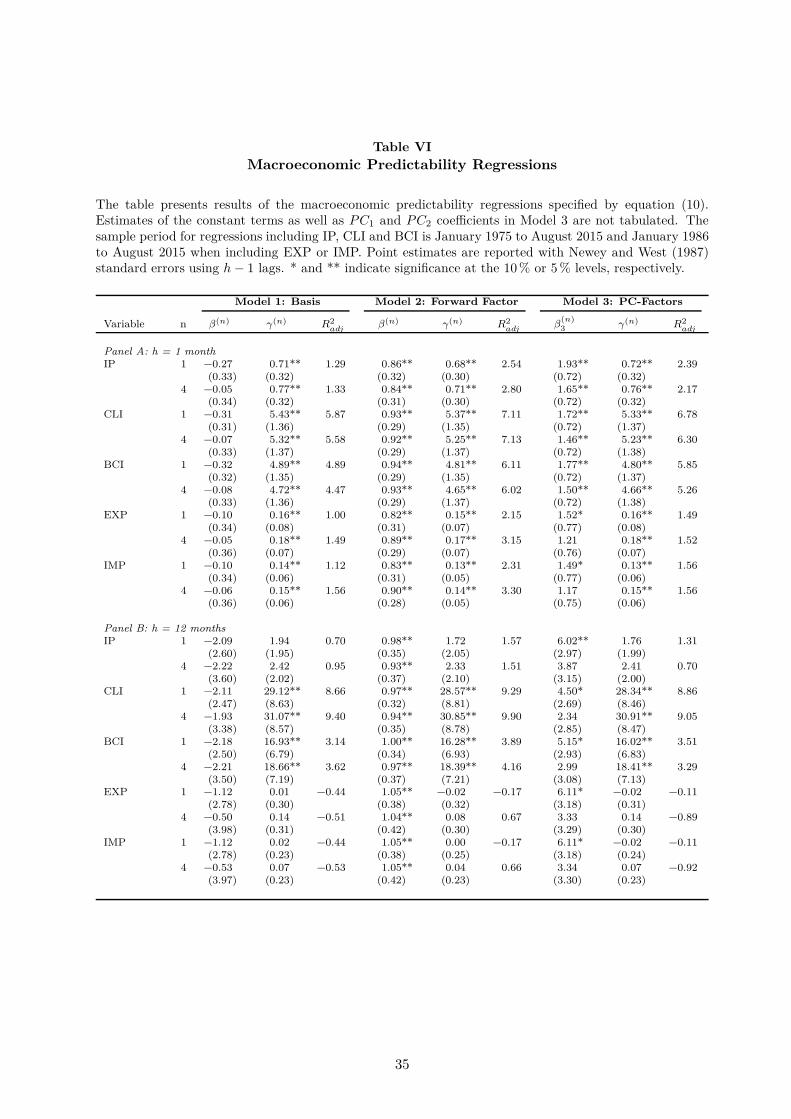
Table VI
Macroeconomic Predictability Regressions
The table presents results of the macroeconomic predictability regressions specified by equation (10).Estimates of the constant terms as well as P C1 and P C2 coefficients in Model 3 are not tabulated. Thesample period for regressions including IP, CLI and BCI is January 1975 to August 2015 and January 1986to August 2015 when including EXP or IMP. Point estimates are reported with Newey and West (1987)standard errors using h − 1 lags. * and ** indicate significance at the 10 % or 5 % levels, respectively.
Model 1: Basis Model 2: Forward Factor Model 3: PC-Factors
Variable n β(n) γ(n) R2adj
β(n) γ(n) R2adj
β(n)3 γ(n) R2
adj
Panel A: h = 1 month
IP 1 −0.27 0.71** 1.29 0.86** 0.68** 2.54 1.93** 0.72** 2.39(0.33) (0.32) (0.32) (0.30) (0.72) (0.32)
4 −0.05 0.77** 1.33 0.84** 0.71** 2.80 1.65** 0.76** 2.17(0.34) (0.32) (0.31) (0.30) (0.72) (0.32)
CLI 1 −0.31 5.43** 5.87 0.93** 5.37** 7.11 1.72** 5.33** 6.78(0.31) (1.36) (0.29) (1.35) (0.72) (1.37)
4 −0.07 5.32** 5.58 0.92** 5.25** 7.13 1.46** 5.23** 6.30(0.33) (1.37) (0.29) (1.37) (0.72) (1.38)
BCI 1 −0.32 4.89** 4.89 0.94** 4.81** 6.11 1.77** 4.80** 5.85(0.32) (1.35) (0.29) (1.35) (0.72) (1.37)
4 −0.08 4.72** 4.47 0.93** 4.65** 6.02 1.50** 4.66** 5.26(0.33) (1.36) (0.29) (1.37) (0.72) (1.38)
EXP 1 −0.10 0.16** 1.00 0.82** 0.15** 2.15 1.52* 0.16** 1.49(0.34) (0.08) (0.31) (0.07) (0.77) (0.08)
4 −0.05 0.18** 1.49 0.89** 0.17** 3.15 1.21 0.18** 1.52(0.36) (0.07) (0.29) (0.07) (0.76) (0.07)
IMP 1 −0.10 0.14** 1.12 0.83** 0.13** 2.31 1.49* 0.13** 1.56(0.34) (0.06) (0.31) (0.05) (0.77) (0.06)
4 −0.06 0.15** 1.56 0.90** 0.14** 3.30 1.17 0.15** 1.56(0.36) (0.06) (0.28) (0.05) (0.75) (0.06)
Panel B: h = 12 months
IP 1 −2.09 1.94 0.70 0.98** 1.72 1.57 6.02** 1.76 1.31(2.60) (1.95) (0.35) (2.05) (2.97) (1.99)
4 −2.22 2.42 0.95 0.93** 2.33 1.51 3.87 2.41 0.70(3.60) (2.02) (0.37) (2.10) (3.15) (2.00)
CLI 1 −2.11 29.12** 8.66 0.97** 28.57** 9.29 4.50* 28.34** 8.86(2.47) (8.63) (0.32) (8.81) (2.69) (8.46)
4 −1.93 31.07** 9.40 0.94** 30.85** 9.90 2.34 30.91** 9.05(3.38) (8.57) (0.35) (8.78) (2.85) (8.47)
BCI 1 −2.18 16.93** 3.14 1.00** 16.28** 3.89 5.15* 16.02** 3.51(2.50) (6.79) (0.34) (6.93) (2.93) (6.83)
4 −2.21 18.66** 3.62 0.97** 18.39** 4.16 2.99 18.41** 3.29(3.50) (7.19) (0.37) (7.21) (3.08) (7.13)
EXP 1 −1.12 0.01 −0.44 1.05** −0.02 −0.17 6.11* −0.02 −0.11(2.78) (0.30) (0.38) (0.32) (3.18) (0.31)
4 −0.50 0.14 −0.51 1.04** 0.08 0.67 3.33 0.14 −0.89(3.98) (0.31) (0.42) (0.30) (3.29) (0.30)
IMP 1 −1.12 0.02 −0.44 1.05** 0.00 −0.17 6.11* −0.02 −0.11(2.78) (0.23) (0.38) (0.25) (3.18) (0.24)
4 −0.53 0.07 −0.53 1.05** 0.04 0.66 3.34 0.07 −0.92(3.97) (0.23) (0.42) (0.23) (3.30) (0.23)
35
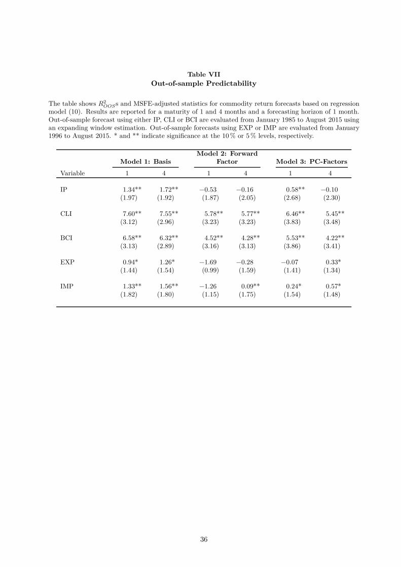
Table VII
Out-of-sample Predictability
The table shows R2OOSs and MSFE-adjusted statistics for commodity return forecasts based on regression
model (10). Results are reported for a maturity of 1 and 4 months and a forecasting horizon of 1 month.Out-of-sample forecast using either IP, CLI or BCI are evaluated from January 1985 to August 2015 usingan expanding window estimation. Out-of-sample forecasts using EXP or IMP are evaluated from January1996 to August 2015. * and ** indicate significance at the 10 % or 5 % levels, respectively.
Model 2: Forward
Model 1: Basis Factor Model 3: PC-Factors
Variable 1 4 1 4 1 4
IP 1.34** 1.72** −0.53 −0.16 0.58** −0.10(1.97) (1.92) (1.87) (2.05) (2.68) (2.30)
CLI 7.60** 7.55** 5.78** 5.77** 6.46** 5.45**(3.12) (2.96) (3.23) (3.23) (3.83) (3.48)
BCI 6.58** 6.32** 4.52** 4.28** 5.53** 4.22**(3.13) (2.89) (3.16) (3.13) (3.86) (3.41)
EXP 0.94* 1.26* −1.69 −0.28 −0.07 0.33*(1.44) (1.54) (0.99) (1.59) (1.41) (1.34)
IMP 1.33** 1.56** −1.26 0.09** 0.24* 0.57*(1.82) (1.80) (1.15) (1.75) (1.54) (1.48)
36
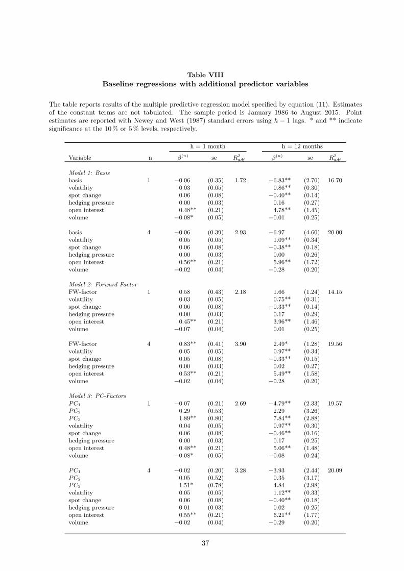
Table VIII
Baseline regressions with additional predictor variables
The table reports results of the multiple predictive regression model specified by equation (11). Estimatesof the constant terms are not tabulated. The sample period is January 1986 to August 2015. Pointestimates are reported with Newey and West (1987) standard errors using h − 1 lags. * and ** indicatesignificance at the 10 % or 5 % levels, respectively.
h = 1 month h = 12 months
Variable n β(n) se R2adj β(n) se R2
adj
Model 1: Basisbasis 1 −0.06 (0.35) 1.72 −6.83** (2.70) 16.70volatility 0.03 (0.05) 0.86** (0.30)spot change 0.06 (0.08) −0.40** (0.14)hedging pressure 0.00 (0.03) 0.16 (0.27)open interest 0.48** (0.21) 4.78** (1.45)volume −0.08* (0.05) −0.01 (0.25)
basis 4 −0.06 (0.39) 2.93 −6.97 (4.60) 20.00volatility 0.05 (0.05) 1.09** (0.34)spot change 0.06 (0.08) −0.38** (0.18)hedging pressure 0.00 (0.03) 0.00 (0.26)open interest 0.56** (0.21) 5.96** (1.72)volume −0.02 (0.04) −0.28 (0.20)
Model 2: Forward FactorFW-factor 1 0.58 (0.43) 2.18 1.66 (1.24) 14.15volatility 0.03 (0.05) 0.75** (0.31)spot change 0.06 (0.08) −0.33** (0.14)hedging pressure 0.00 (0.03) 0.17 (0.29)open interest 0.45** (0.21) 3.96** (1.46)volume −0.07 (0.04) 0.01 (0.25)
FW-factor 4 0.83** (0.41) 3.90 2.49* (1.28) 19.56volatility 0.05 (0.05) 0.97** (0.34)spot change 0.05 (0.08) −0.33** (0.15)hedging pressure 0.00 (0.03) 0.02 (0.27)open interest 0.53** (0.21) 5.49** (1.58)volume −0.02 (0.04) −0.28 (0.20)
Model 3: PC-FactorsP C1 1 −0.07 (0.21) 2.69 −4.79** (2.33) 19.57P C2 0.29 (0.53) 2.29 (3.26)P C3 1.89** (0.80) 7.84** (2.88)volatility 0.04 (0.05) 0.97** (0.30)spot change 0.06 (0.08) −0.46** (0.16)hedging pressure 0.00 (0.03) 0.17 (0.25)open interest 0.48** (0.21) 5.06** (1.48)volume −0.08* (0.05) −0.08 (0.24)
P C1 4 −0.02 (0.20) 3.28 −3.93 (2.44) 20.09P C2 0.05 (0.52) 0.35 (3.17)P C3 1.51* (0.78) 4.84 (2.98)volatility 0.05 (0.05) 1.12** (0.33)spot change 0.06 (0.08) −0.40** (0.18)hedging pressure 0.01 (0.03) 0.02 (0.25)open interest 0.55** (0.21) 6.21** (1.77)volume −0.02 (0.04) −0.29 (0.20)
37
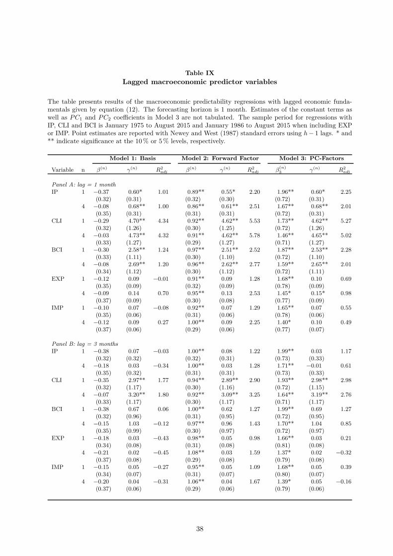
Table IX
Lagged macroeconomic predictor variables
The table presents results of the macroeconomic predictability regressions with lagged economic funda-mentals given by equation (12). The forecasting horizon is 1 month. Estimates of the constant terms aswell as P C1 and P C2 coefficients in Model 3 are not tabulated. The sample period for regressions withIP, CLI and BCI is January 1975 to August 2015 and January 1986 to August 2015 when including EXPor IMP. Point estimates are reported with Newey and West (1987) standard errors using h − 1 lags. * and** indicate significance at the 10 % or 5 % levels, respectively.
Model 1: Basis Model 2: Forward Factor Model 3: PC-Factors
Variable n β(n) γ(n) R2adj β(n) γ(n) R2
adj β(n)3 γ(n) R2
adj
Panel A: lag = 1 monthIP 1 −0.37 0.60* 1.01 0.89** 0.55* 2.20 1.96** 0.60* 2.25
(0.32) (0.31) (0.32) (0.30) (0.72) (0.31)4 −0.08 0.68** 1.00 0.86** 0.61** 2.51 1.67** 0.68** 2.01
(0.35) (0.31) (0.31) (0.31) (0.72) (0.31)CLI 1 −0.29 4.70** 4.34 0.92** 4.62** 5.53 1.73** 4.62** 5.27
(0.32) (1.26) (0.30) (1.25) (0.72) (1.26)4 −0.03 4.73** 4.32 0.91** 4.62** 5.78 1.46** 4.65** 5.02
(0.33) (1.27) (0.29) (1.27) (0.71) (1.27)BCI 1 −0.30 2.58** 1.24 0.97** 2.51** 2.52 1.87** 2.53** 2.28
(0.33) (1.11) (0.30) (1.10) (0.72) (1.10)4 −0.08 2.69** 1.20 0.96** 2.62** 2.77 1.59** 2.65** 2.01
(0.34) (1.12) (0.30) (1.12) (0.72) (1.11)EXP 1 −0.12 0.09 −0.01 0.91** 0.09 1.28 1.68** 0.10 0.69
(0.35) (0.09) (0.32) (0.09) (0.78) (0.09)4 −0.09 0.14 0.70 0.95** 0.13 2.53 1.45* 0.15* 0.98
(0.37) (0.09) (0.30) (0.08) (0.77) (0.09)IMP 1 −0.10 0.07 −0.08 0.92** 0.07 1.29 1.65** 0.07 0.55
(0.35) (0.06) (0.31) (0.06) (0.78) (0.06)4 −0.12 0.09 0.27 1.00** 0.09 2.25 1.40* 0.10 0.49
(0.37) (0.06) (0.29) (0.06) (0.77) (0.07)
Panel B: lag = 3 monthsIP 1 −0.38 0.07 −0.03 1.00** 0.08 1.22 1.99** 0.03 1.17
(0.32) (0.32) (0.32) (0.31) (0.73) (0.33)4 −0.18 0.03 −0.34 1.00** 0.03 1.28 1.71** −0.01 0.61
(0.35) (0.32) (0.31) (0.31) (0.73) (0.33)CLI 1 −0.35 2.97** 1.77 0.94** 2.89** 2.90 1.93** 2.98** 2.98
(0.32) (1.17) (0.30) (1.16) (0.72) (1.15)4 −0.07 3.20** 1.80 0.92** 3.09** 3.25 1.64** 3.19** 2.76
(0.33) (1.17) (0.30) (1.17) (0.71) (1.17)BCI 1 −0.38 0.67 0.06 1.00** 0.62 1.27 1.99** 0.69 1.27
(0.32) (0.96) (0.31) (0.95) (0.72) (0.95)4 −0.15 1.03 −0.12 0.97** 0.96 1.43 1.70** 1.04 0.85
(0.35) (0.99) (0.30) (0.97) (0.72) (0.97)EXP 1 −0.18 0.03 −0.43 0.98** 0.05 0.98 1.66** 0.03 0.21
(0.34) (0.08) (0.31) (0.08) (0.81) (0.08)4 −0.21 0.02 −0.45 1.08** 0.03 1.59 1.37* 0.02 −0.32
(0.37) (0.08) (0.29) (0.08) (0.79) (0.08)IMP 1 −0.15 0.05 −0.27 0.95** 0.05 1.09 1.68** 0.05 0.39
(0.34) (0.07) (0.31) (0.07) (0.80) (0.07)4 −0.20 0.04 −0.31 1.06** 0.04 1.67 1.39* 0.05 −0.16
(0.37) (0.06) (0.29) (0.06) (0.79) (0.06)
38
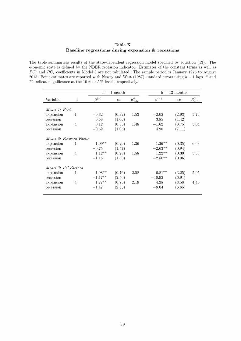
Table X
Baseline regressions during expansion & recessions
The table summarizes results of the state-dependent regression model specified by equation (13). Theeconomic state is defined by the NBER recession indicator. Estimates of the constant terms as well asP C1 and P C2 coefficients in Model 3 are not tabulated. The sample period is January 1975 to August2015. Point estimates are reported with Newey and West (1987) standard errors using h − 1 lags. * and** indicate significance at the 10 % or 5 % levels, respectively.
h = 1 month h = 12 months
Variable n β(n) se R2adj β(n) se R2
adj
Model 1: Basisexpansion 1 −0.32 (0.32) 1.53 −2.02 (2.93) 5.76recession 0.58 (1.06) 3.85 (4.42)expansion 4 0.12 (0.35) 1.48 −1.62 (3.75) 5.04recession −0.52 (1.05) 4.90 (7.11)
Model 2: Forward Factorexpansion 1 1.09** (0.29) 1.36 1.26** (0.35) 6.63recession −0.75 (1.57) −2.63** (0.94)expansion 4 1.12** (0.28) 1.58 1.22** (0.39) 5.58recession −1.15 (1.53) −2.50** (0.96)
Model 3: PC-Factorsexpansion 1 1.98** (0.76) 2.58 6.81** (3.25) 5.95recession −1.17** (2.56) −10.92 (6.91)expansion 4 1.77** (0.75) 2.19 4.28 (3.58) 4.46recession −1.47 (2.55) −8.04 (6.65)
39
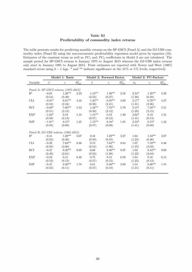
Table XI
Predictability of commodity index returns
The table presents results for predicting monthly returns on the SP-GSCI (Panel A) and the DJ-UBS com-modity index (Panel B) using the macroeconomic predictability regression model given by equation (10).Estimates of the constant terms as well as P C1 and P C2 coefficients in Model 3 are not tabulated. Thesample period for SP-GSCI returns is January 1975 to August 2015 whereas the DJ-UBS index returnsonly start in January 1991 to August 2015. Point estimates are reported with Newey and West (1987)standard errors using h − 1 lags. * and ** indicate significance at the 10 % or 5 % levels, respectively.
Model 1: Basis Model 2: Forward Factor Model 3: PC-Factors
Variable β γ R2adj β γ R2
adj β3 γ R2adj
Panel A: SP-GSCI returns (1975-2015)IP −0.85 1.26** 2.23 1.13** 1.30** 2.58 2.34* 1.28** 2.28
(0.54) (0.49) (0.53) (0.47) (1.30) (0.49)CLI −0.91* 6.81** 4.42 1.33** 6.95** 4.69 2.17* 6.76** 4.37
(0.52) (2.24) (0.50) (2.21) (1.31) (2.26)BCI −0.89* 7.60** 5.53 1.32** 7.70** 5.79 2.15* 7.58** 5.51
(0.51) (2.13) (0.50) (2.12) (1.29) (2.15)EXP −1.02* 0.18 1.18 1.15** 0.19 1.30 2.62* 0.19 1.21
(0.58) (0.13) (0.57) (0.12) (1.41) (0.13)IMP −1.01* 0.15* 1.25 1.15** 0.16* 1.35 2.53* 0.15* 1.22
(0.58) (0.09) (0.57) (0.09) (1.41) (0.09)
Panel B: DJ-UBS returns (1991-2015)IP −0.41 1.28** 3.07 0.44 1.29** 3.27 1.64 1.34** 3.07
(0.52) (0.46) (0.59) (0.45) (1.23) (0.46)CLI −0.39 7.63** 8.86 0.72 7.63** 9.04 1.07 7.59** 8.46
(0.50) (2.00) (0.54) (1.96) (1.25) (2.03)BCI −0.37 8.39** 9.89 0.66 8.36** 9.97 1.03 8.42** 9.60
(0.49) (2.01) (0.53) (1.98) (1.22) (2.04)EXP −0.53 0.15 0.40 0.75 0.15 0.59 1.64 0.16 0.15
(0.52) (0.12) (0.57) (0.12) (1.22) (0.12)IMP −0.47 0.26** 1.78 0.61 0.26** 2.00 1.54 0.26** 1.55
(0.52) (0.11) (0.57) (0.10) (1.21) (0.11)
40
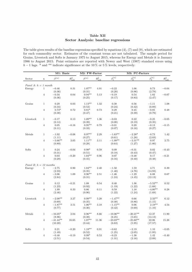
Table XII
Sector Analysis: baseline regressions
The table gives results of the baseline regressions specified by equations (4), (7) and (9), which are estimatedfor each commodity sector. Estimates of the constant terms are not tabulated. The sample period forGrains, Livestock and Softs is January 1975 to August 2015, whereas for Energy and Metals it is January1986 to August 2015. Point estimates are reported with Newey and West (1987) standard errors usingh − 1 lags. * and ** indicate significance at the 10 % or 5 % levels, respectively.
M1: Basis M2: FW-Factor M3: PC-Factors
Sector n β(n) R2adj
β(n) R2adj
β(n)1 β
(n)2 β
(n)3 R2
adj
Panel A: h = 1 month
Energy 1 −0.46 0.31 1.07** 4.91 −0.22 1.06 0.73 −0.04(0.36) (0.31) (0.20) (0.96) (2.79)
4 −0.34 0.04 0.94** 5.13 −0.19 0.54 1.82 −0.07(0.36) (0.25) (0.17) (0.83) (2.47)
Grains 1 0.29 0.03 1.13** 1.32 0.38 0.56 −1.11 1.08(0.34) (0.53) (0.24) (0.42) (0.89)
4 0.73* 0.72 0.81* 0.73 0.29 0.45 −0.85 0.48(0.38) (0.47) (0.21) (0.39) (0.79)
Livestock 1 −0.17 0.13 1.09** 1.36 −0.03 0.22 −0.25 −0.05(0.14) (0.39) (0.08) (0.19) (0.35)
4 0.05 −0.16 0.95** 0.79 −0.01 0.20 −0.13 −0.15(0.11) (0.33) (0.07) (0.16) (0.27)
Metals 1 −1.02 −0.08 0.97** 2.29 −1.63** −2.28* −0.73 1.42(1.11) (0.27) (0.61) (1.28) (2.03)
4 −3.66** 3.05 1.11** 3.11 −1.99** −3.31** 0.97 2.75(0.89) (0.28) (0.64) (1.27) (1.80)
Softs 1 0.24 −0.04 0.98* 0.59 0.09 −0.31 0.02 −0.43(0.31) (0.51) (0.18) (0.43) (0.47)
4 0.03 −0.20 1.04** 0.96 0.07 −0.48 0.17 −0.21(0.29) (0.45) (0.16) (0.40) (0.48)
Panel B: h = 12 months
Energy 1 −2.75 0.90 1.04** 2.40 −1.50 1.59 4.71 0.39(2.33) (0.35) (1.40) (4.76) (14.93)
4 −3.06 1.09 0.96** 2.51 −1.46 −1.29 6.08 0.67(2.84) (0.31) (1.24) (4.45) (12.13)
Grains 1 0.12 −0.21 1.08 0.54 0.40 1.36 −5.52** 0.52(1.23) (0.92) (1.19) (1.22) (1.68)
4 1.99 0.33 0.86 0.11 0.59 1.18 −4.80** 0.28(2.46) (0.90) (1.22) (1.24) (1.69)
Livestock 1 −2.08** 3.27 0.99** 5.28 −1.47** 0.66 2.33** 6.12(0.69) (0.35) (0.48) (0.86) (1.15)
4 −1.87** 3.51 1.06** 3.18 −1.15** 0.06 2.18** 4.54(0.77) (0.30) (0.42) (0.69) (1.10)
Metals 1 −16.05* 2.04 0.96** 8.66 −19.06** −20.21** 12.37 11.90(8.96) (0.38) (6.25) (5.65) (14.13)
4 −41.44** 16.65 1.07** 11.36 −23.03** −25.60** 22.06 15.26(10.20) (0.44) (6.63) (5.95) (17.57)
Softs 1 0.21 −0.20 1.18** 0.91 −0.62 −2.19 1.10 −0.05(1.49) (0.52) (1.25) (2.05) (1.95)
4 −0.48 −0.19 0.99* 0.53 −0.23 −1.38 1.42 −0.40(2.51) (0.54) (1.31) (2.16) (2.09)
41
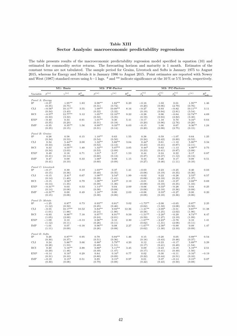
Table XIII
Sector Analysis: macroeconomic predictability regressions
The table presents results of the macroeconomic predictability regression model specified in equation (10) andestimated for commodity sector returns. The forecasting horizon and maturity is 1 month. Estimates of theconstant terms are not tabulated. The sample period for Grains, Livestock and Softs is January 1975 to August2015, whereas for Energy and Metals it is January 1986 to August 2015. Point estimates are reported with Neweyand West (1987) standard errors using h−1 lags. * and ** indicate significance at the 10 % or 5 % levels, respectively.
M1: Basis M2: FW-Factor M3: PC-Factors
Variable β(n) γ(n) R2adj
β(n) γ(n) R2adj
β(n)1
β(n)2
β(n)3
γ(n) R2adj
Panel A: Energy
IP −0.37 1.95** 1.83 0.98** 1.82** 6.29 −0.16 1.02 0.01 1.95** 1.46(0.35) (0.75) (0.31) (0.72) (0.20) (0.96) (2.79) (0.76)
CLI −0.56* 10.11** 3.55 1.09** 10.09** 8.16 −0.27 0.93 −0.82 10.11** 3.11(0.34) (3.43) (0.32) (3.32) (0.19) (0.94) (2.81) (3.54)
BCI −0.57* 12.77** 5.12 1.05** 12.10** 9.22 −0.28 0.96 −0.64 12.74** 4.69(0.33) (3.32) (0.32) (3.35) (0.19) (0.94) (2.82) (3.40)
EXP −0.40 0.33 0.91 1.01** 0.30 5.41 −0.17 1.18 0.70 0.34* 0.64(0.35) (0.20) (0.31) (0.18) (0.20) (0.96) (2.76) (0.20)
IMP −0.35 0.35** 1.56 0.99** 0.33** 6.03 −0.15 1.06 0.67 0.36** 1.24(0.35) (0.15) (0.31) (0.14) (0.20) (0.98) (2.75) (0.15)
Panel B: Grains
IP 0.28 0.58 0.15 1.18** 0.63 1.55 0.38 0.59 −1.07 0.64 1.25(0.34) (0.53) (0.54) (0.50) (0.24) (0.42) (0.89) (0.53)
CLI 0.34 5.44** 2.00 1.32** 5.88** 3.64 0.44* 0.61 −1.10 5.80** 3.34(0.33) (2.06) (0.52) (2.12) (0.23) (0.41) (0.87) (2.11)
BCI 0.33 4.55** 1.40 1.32** 5.07** 3.05 0.44* 0.62 −1.13 4.99** 2.75(0.34) (2.03) (0.53) (2.09) (0.23) (0.41) (0.87) (2.08)
EXP 0.49 0.18 0.71 1.01* 0.17 1.53 0.44 0.24 0.22 0.17 0.87(0.41) (0.14) (0.60) (0.13) (0.27) (0.47) (1.12) (0.14)
IMP 0.47 0.09 0.33 1.00* 0.08 1.15 0.44 0.26 0.17 0.09 0.51(0.41) (0.10) (0.60) (0.09) (0.27) (0.46) (1.11) (0.10)
Panel C: Livestock
IP −0.17 0.39 0.19 1.03** 0.37 1.41 −0.03 0.23 −0.25 0.40 0.03(0.15) (0.36) (0.40) (0.35) (0.08) (0.19) (0.35) (0.36)
CLI −0.15 2.41* 0.67 1.08** 2.54* 1.99 −0.02 0.22 −0.28 2.53* 0.57(0.14) (1.40) (0.39) (1.41) (0.08) (0.18) (0.35) (1.37)
BCI −0.15 2.56* 0.79 1.08** 2.67* 2.10 −0.01 0.22 −0.27 2.68** 0.69(0.14) (1.35) (0.39) (1.36) (0.08) (0.18) (0.35) (1.33)
EXP −0.31** 0.03 0.53 1.14** 0.04 2.09 −0.06 0.33* −0.28 0.04 0.25(0.14) (0.08) (0.38) (0.08) (0.08) (0.18) (0.36) (0.08)
IMP −0.31** 0.00 0.49 1.16** 0.00 2.03 −0.06 0.33* −0.27 0.00 0.20(0.15) (0.06) (0.38) (0.06) (0.08) (0.18) (0.36) (0.06)
Panel D: Metals
IP −1.25 0.87* 0.73 0.93** 0.81* 3.02 −1.73** −2.08 −0.65 0.87* 2.25(1.12) (0.50) (0.25) (0.46) (0.62) (1.32) (2.08) (0.50)
CLI −0.55 10.17** 10.52 0.84** 9.93** 12.36 −1.21** −2.09* −0.51 9.87** 11.38(1.01) (1.88) (0.24) (1.90) (0.58) (1.25) (2.02) (1.90)
BCI −0.93 8.88** 7.18 0.97** 8.91** 9.59 −1.51** −2.20* −0.29 8.74** 8.47(1.05) (2.00) (0.24) (2.01) (0.59) (1.27) (2.19) (1.99)
EXP −1.09 0.10 −0.13 0.96** 0.10 2.30 −1.67** −2.23* −0.78 0.10 1.41(1.12) (0.11) (0.26) (0.11) (0.62) (1.31) (2.08) (0.11)
IMP −1.01 0.07 −0.18 0.96** 0.08 2.27 −1.67** −2.38* −0.99 0.09 1.47(1.11) (0.09) (0.26) (0.08) (0.62) (1.30) (2.10) (0.09)
Panel E: Softs
IP 0.26 0.87** 0.95 0.78 0.84** 1.46 0.15 −0.20 0.05 0.88** 0.54(0.30) (0.37) (0.51) (0.36) (0.18) (0.43) (0.48) (0.37)
CLI 0.24 5.86** 3.66 0.88* 5.79** 4.20 0.12 −0.23 −0.17 5.89** 3.29(0.28) (1.53) (0.49) (1.51) (0.17) (0.41) (0.49) (1.54)
BCI 0.20 5.16** 2.88 0.88* 5.11** 3.45 0.09 −0.23 −0.18 5.19** 2.51(0.29) (1.48) (0.49) (1.47) (0.17) (0.41) (0.49) (1.50)
EXP −0.14 0.16* 0.29 0.84 0.16* 0.77 0.02 0.30 −0.11 0.16* −0.19(0.31) (0.10) (0.80) (0.09) (0.22) (0.44) (0.51) (0.10)
IMP −0.19 0.15* 0.51 0.85 0.15* 0.97 0.01 0.37 −0.14 0.15* 0.07(0.30) (0.08) (0.79) (0.08) (0.22) (0.43) (0.50) (0.08)
42
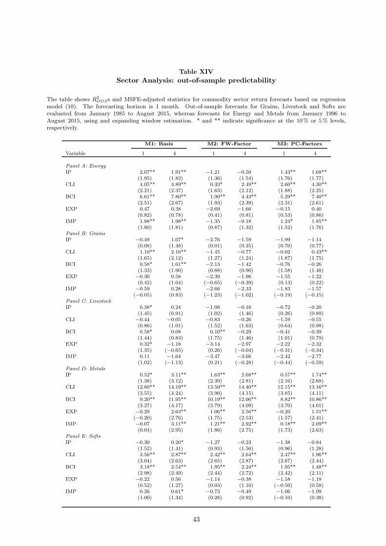
Table XIV
Sector Analysis: out-of-sample predictability
The table shows R2OOSs and MSFE-adjusted statistics for commodity sector return forecasts based on regression
model (10). The forecasting horizon is 1 month. Out-of-sample forecasts for Grains, Livestock and Softs areevaluated from January 1985 to August 2015, whereas forecasts for Energy and Metals from January 1996 toAugust 2015, using and expanding window estimation. * and ** indicate significance at the 10 % or 5 % levels,respectively.
M1: Basis M2: FW-Factor M3: PC-Factors
Variable 1 4 1 4 1 4
Panel A: Energy
IP 2.07** 1.91** −1.21 −0.50 1.43** 1.68**(1.95) (1.82) (1.36) (1.54) (1.76) (1.77)
CLI 4.05** 4.89** 0.33* 2.49** 2.60** 4.30**(2.21) (2.37) (1.63) (2.12) (1.88) (2.25)
BCI 6.61** 7.80** 1.90** 4.43** 5.29** 7.40**(2.51) (2.67) (1.93) (2.39) (2.31) (2.61)
EXP 0.47 0.38 −2.69 −1.66 −0.15 0.40(0.82) (0.78) (0.41) (0.81) (0.53) (0.86)
IMP 1.88** 1.98** −1.35 −0.18 1.24* 1.85**(1.80) (1.81) (0.87) (1.32) (1.52) (1.76)
Panel B: Grains
IP −0.49 1.07* −2.76 −1.59 −1.99 −1.14(0.08) (1.48) (0.01) (0.35) (0.70) (0.77)
CLI 1.10** 2.16** −1.45 −0.77 −0.02 0.43**(1.65) (2.12) (1.27) (1.24) (1.87) (1.75)
BCI 0.58* 1.61** −2.13 −1.42 −0.76 −0.26(1.33) (1.90) (0.88) (0.90) (1.58) (1.48)
EXP −0.30 0.58 −2.39 −1.96 −1.55 −1.22(0.42) (1.04) (−0.65) (−0.39) (0.13) (0.22)
IMP −0.59 0.28 −2.66 −2.33 −1.83 −1.57(−0.05) (0.83) (−1.23) (−1.02) (−0.19) (−0.15)
Panel C: Livestock
IP 0.38* 0.24 −1.08 −0.16 −0.72 −0.20(1.45) (0.91) (1.02) (1.46) (0.26) (0.89)
CLI −0.44 −0.05 −0.83 −0.26 −1.59 −0.55(0.86) (1.01) (1.52) (1.63) (0.64) (0.98)
BCI 0.58* 0.08 0.10** −0.29 −0.41 −0.39(1.44) (0.83) (1.75) (1.46) (1.01) (0.79)
EXP 0.32* −1.18 −3.14 −2.97 −2.22 −2.32(1.35) (−0.65) (0.26) (−0.04) (−0.31) (−0.34)
IMP 0.11 −1.64 −3.47 −3.66 −2.42 −2.77(1.02) (−1.13) (0.21) (−0.28) (−0.44) (−0.59)
Panel D: Metals
IP 0.52* 3.11** 1.63** 2.68** 0.57** 1.74**(1.38) (3.12) (2.39) (2.81) (2.16) (2.68)
CLI 12.80** 14.19** 13.50** 14.40** 12.15** 13.16**(3.55) (4.24) (3.90) (4.15) (3.85) (4.11)
BCI 9.20** 11.95** 10.19** 12.06** 8.82** 10.86**(3.27) (4.17) (3.79) (4.09) (3.70) (4.01)
EXP −0.29 2.63** 1.06** 2.56** −0.20 1.51**(−0.20) (2.76) (1.75) (2.53) (1.57) (2.41)
IMP −0.07 3.11** 1.21** 2.92** 0.18** 2.09**(0.04) (2.95) (1.86) (2.75) (1.73) (2.63)
Panel E: Softs
IP −0.30 0.20* −1.27 −0.23 −1.38 −0.84(1.52) (1.41) (0.93) (1.56) (0.96) (1.28)
CLI 3.56** 2.87** 2.42** 2.64** 2.47** 1.96**(3.04) (2.63) (2.65) (2.87) (2.67) (2.44)
BCI 3.18** 2.54** 1.95** 2.24** 1.95** 1.48**(2.98) (2.49) (2.44) (2.72) (2.42) (2.11)
EXP −0.22 0.56 −1.14 −0.38 −1.58 −1.18(0.52) (1.27) (0.03) (1.10) (−0.50) (0.58)
IMP 0.26 0.61* −0.73 −0.49 −1.06 −1.09(1.00) (1.34) (0.28) (0.92) (−0.10) (0.38)
43
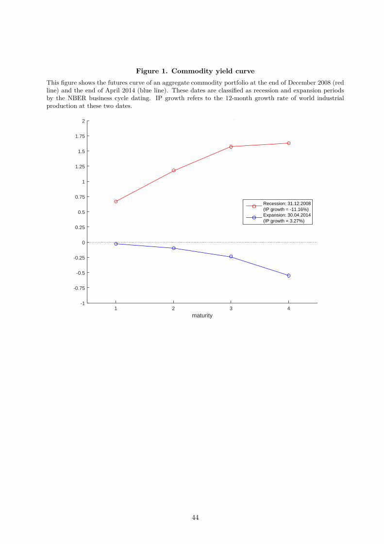
Figure 1. Commodity yield curve
This figure shows the futures curve of an aggregate commodity portfolio at the end of December 2008 (redline) and the end of April 2014 (blue line). These dates are classified as recession and expansion periodsby the NBER business cycle dating. IP growth refers to the 12-month growth rate of world industrialproduction at these two dates.
maturity1 2 3 4
-1
-0.75
-0.5
-0.25
0
0.25
0.5
0.75
1
1.25
1.5
1.75
2Term structure of Commodity Basis
Recession: 31.12.2008(IP growth = -11.16%)Expansion: 30.04.2014(IP growth = 3.27%)
44
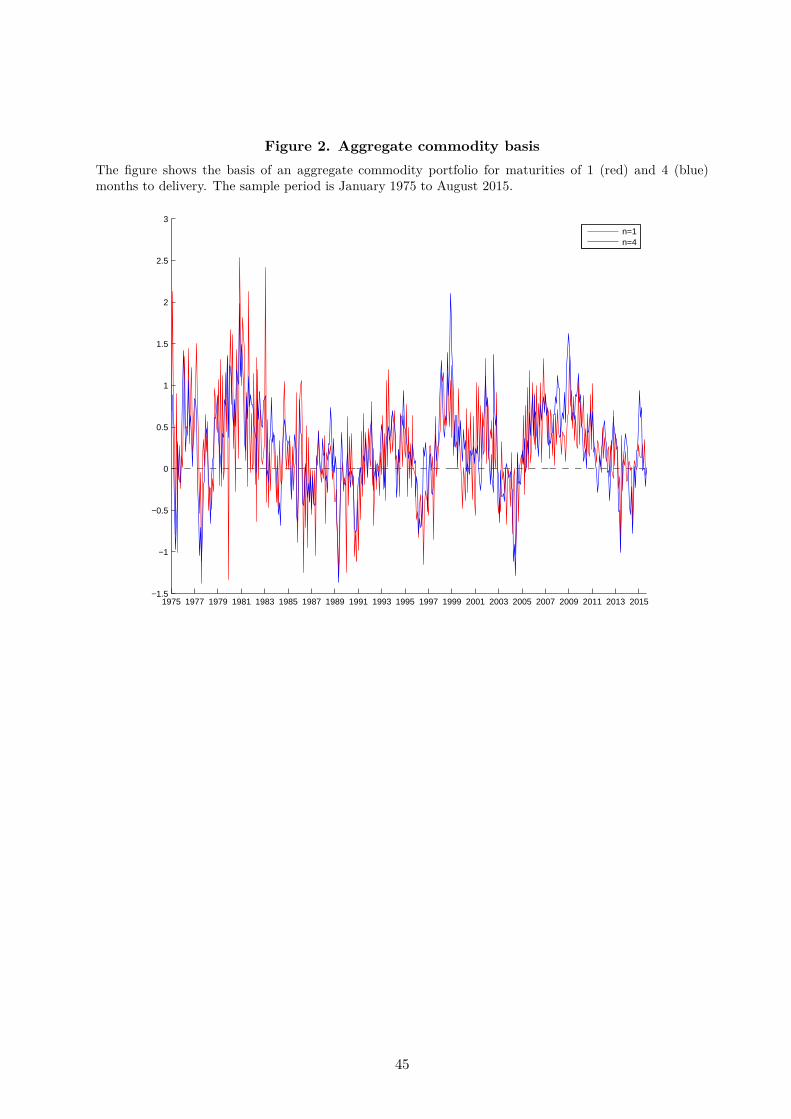
Figure 2. Aggregate commodity basis
The figure shows the basis of an aggregate commodity portfolio for maturities of 1 (red) and 4 (blue)months to delivery. The sample period is January 1975 to August 2015.
1975 1977 1979 1981 1983 1985 1987 1989 1991 1993 1995 1997 1999 2001 2003 2005 2007 2009 2011 2013 2015−1.5
−1
−0.5
0
0.5
1
1.5
2
2.5
3Basis
n=1n=4
45
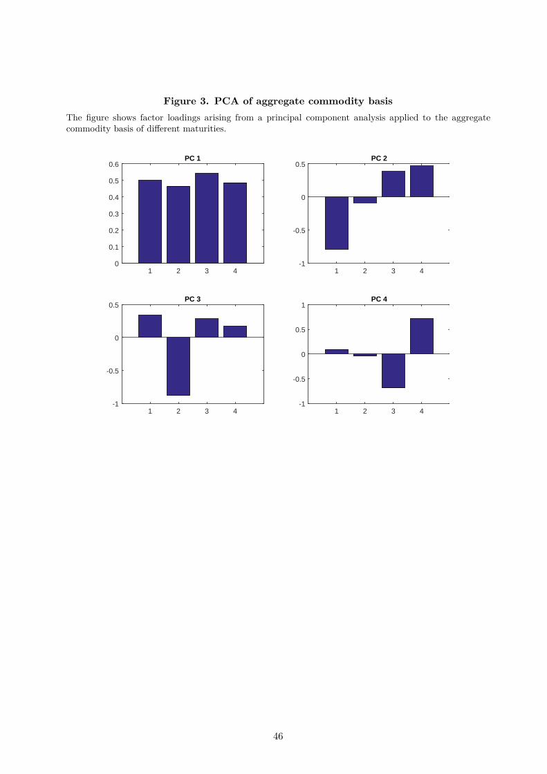
Figure 3. PCA of aggregate commodity basis
The figure shows factor loadings arising from a principal component analysis applied to the aggregatecommodity basis of different maturities.
1 2 3 40
0.1
0.2
0.3
0.4
0.5
0.6PC 1
1 2 3 4-1
-0.5
0
0.5PC 2
1 2 3 4-1
-0.5
0
0.5PC 3
(Basis, 1975)
1 2 3 4-1
-0.5
0
0.5
1PC 4
46
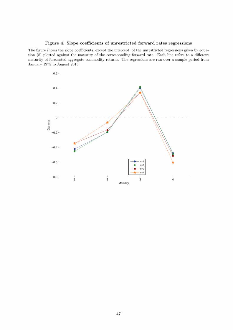
Figure 4. Slope coefficients of unrestricted forward rates regressions
The figure shows the slope coefficients, except the intercept, of the unrestricted regressions given by equa-tion (8) plotted against the maturity of the corresponding forward rate. Each line refers to a differentmaturity of forecasted aggregate commodity returns. The regressions are run over a sample period fromJanuary 1975 to August 2015.
1 2 3 4−0.8
−0.6
−0.4
−0.2
0
0.2
0.4
0.6
Maturity
Gam
ma
n=1
n=2
n=3
n=4
47
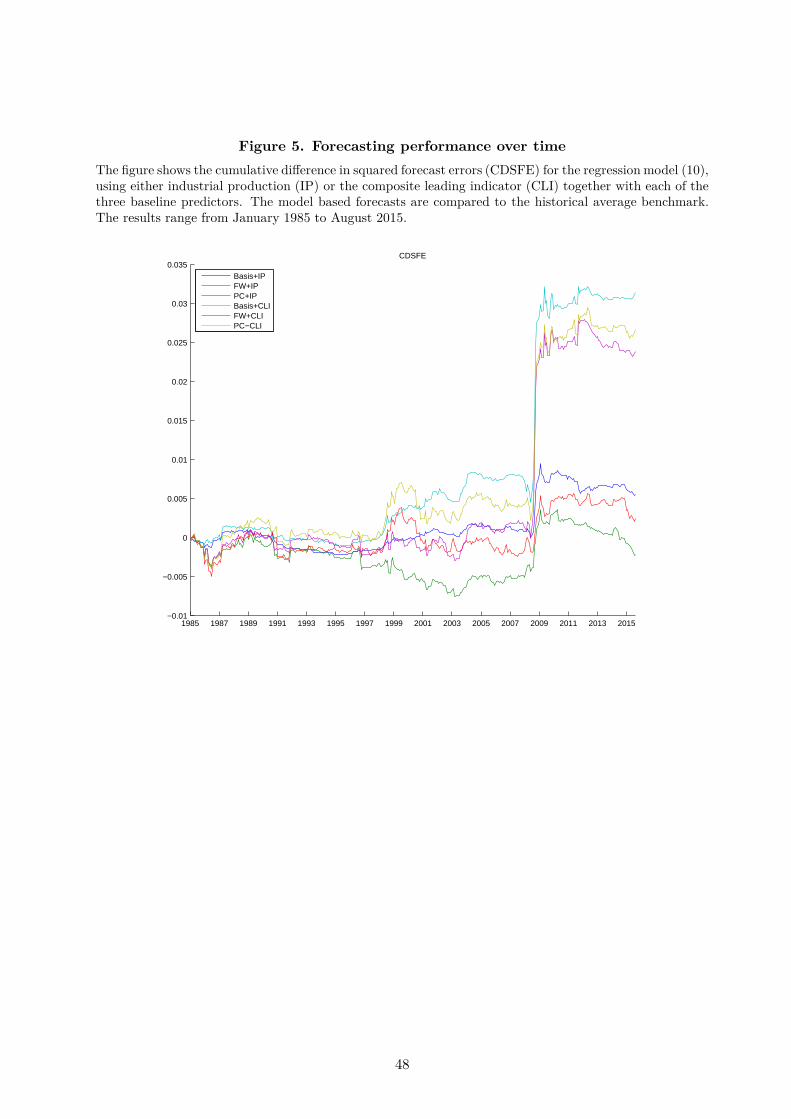
Figure 5. Forecasting performance over time
The figure shows the cumulative difference in squared forecast errors (CDSFE) for the regression model (10),using either industrial production (IP) or the composite leading indicator (CLI) together with each of thethree baseline predictors. The model based forecasts are compared to the historical average benchmark.The results range from January 1985 to August 2015.
1985 1987 1989 1991 1993 1995 1997 1999 2001 2003 2005 2007 2009 2011 2013 2015−0.01
−0.005
0
0.005
0.01
0.015
0.02
0.025
0.03
0.035CDSFE
Basis+IPFW+IPPC+IPBasis+CLIFW+CLIPC−CLI
48