Richardson Extrapolation-based DiscretizationUncertainty Estimation for Computational Fluid

Dynamics

Tyrone S. PhillipsGraduate Research Assistant

Department of Aerospace and Ocean EngineeringVirginia Tech

Blacksburg, Virginia 24061Email: tphilli6@vt.edu

Christopher J. RoyProfessor

Department of Aerospace and Ocean EngineeringVirginia Tech

Blacksburg, Virginia 24061Email: cjroy@vt.edu

ABSTRACT

This study investigates the accuracy of various Richardson extrapolation-based discretization error and un-certainty estimators for problems in computational fluid dynamics. Richardson extrapolation uses two solutionson systematically refined grids to estimate the exact solution to the partial differential equations and is accurateonly in the asymptotic range (i.e., when the grids are sufficiently fine). The uncertainty estimators investigated arevariations of the Grid Convergence Index and include a globally averaged observed order of accuracy, the Factorof Safety method, the Correction Factor method, and Least-Squares methods. Several 2D and 3D applications tothe Euler, Navier-Stokes, and Reynolds-Averaged Navier-Stokes with exact solutions and a 2D turbulent flat platewith a numerical benchmark are used to evaluate the uncertainty estimators. Local solution quantities (e.g. density,velocity, and pressure) have much slower grid convergence on coarser meshes than global quantities resulting innon-asymptotic solutions and inaccurate Richardson extrapolation error estimates; however, an uncertainty esti-mate may still be required. The uncertainty estimators are applied to local solution quantities to evaluate accuracyfor all possible types of convergence rates. Extensions were added where necessary for treatment of cases wherethe local convergence rate is oscillatory or divergent. The conservativeness and effectivity of the discretizationuncertainty estimators are used to assess the relative merits of the different approaches.

1 IntroductionComputational Fluid Dynamics, or CFD, has enormous potential to impact the analysis, design, and optimization of

engineering systems. The predictive capability of CFD depends not only on the validity of the sub-models employed (e.g.,turbulence, chemistry, multi-phase flow) and the uncertainties present in the system and surroundings, but also on the abilityto reliably estimate and reduce numerical errors. While there are several sources of numerical error in a CFD computation,the largest and most difficult to estimate is usually the error related to the resolution of the spatial grid, i.e., the spatialdiscretization error.

For a solution solved on a grid with spacing h, the discretization error, εh, is defined as the difference between the exactsolution to the discrete equations, uh, and the exact solution to the PDEs, u,

εh = uh− u. (1)

1

Accepted in ASME Journal of Fluids Engineering, 2014

The exact exact solution to the discrete equations, uh, assumes that round-off error, iterative error, and other sources ofnumerical error are zero (or negligible relative to discretization error). Richardson extrapolation uses a sequence of solutionsto estimate discretization error and can be applied to almost any type of computational simulation as well as to both localand global quantities. The method is not code intrusive and is applied as a post processing step. For smooth solutions withno discontinuities, the exact solution can be written in terms of a power series expansion, u = uh−∑

∞p=p f

αphp, which canbe used to rewrite Eq. 1 as

εh =∞

∑p=p f

αphp = αp f hp f +HOT. (2)

For a fully verified code, the formal order of accuracy, p f , is determined by the chosen discretization scheme and is theexponent of the first term in the series. If discontinuities are present, the formal order of the discretization scheme is reduced.A formal order of one is expected for a non-linear discontinuity and ps/(ps + 1) for a linear discontinuity where ps is theformal order for a smooth problem, see Banks et al. [1] for more discussion. To reasonably approximate the discretizationerror, the Higher Order Terms (HOT) are dropped reducing Eq. 2 to

εh ≈ εh = αp f hp f . (3)

The exclusion of the HOT introduces the assumption that numeric solutions are asymptotic (i.e., HOT � αp f hp f ) forthe estimated discretization error, εh, to accurately approximate the true discretization error, εh. Richardson extrapolationis formulated to solve for the unknowns in Eq. 3, αp f and εh, using solutions on two systematically refined grids (see dis-cussion in Section 2). This further extends the requirement of an asymptotic solution to not only the solution on which thediscretization error is to be estimated but also to any additional solutions used in the extrapolation. In practice, for Eq. 3 tobe accurate, all sources of numerical error must be negligible relative to discretization error, the solver should be verifiedto match the expected order of accuracy of the discretization scheme, and the two numerical solutions used to estimate thediscretization error must be asymptotic. (While not accurate for a power series expansion, Richardson extrapolation can beapplied to a solution with discontinuities but the expected order of accuracy is reduced from what would be found for smoothproblems.) If any of the assumptions are not met, then the solution can exhibit a different order of convergence and a differenttype of convergence toward the exact solution. The observed order of accuracy requires three solutions on systematicallyrefined grids to compute and is related to four different types of convergence: monotonic convergence, monotonic diver-gence, oscillatory convergence, and oscillatory divergence. Monotonic convergence and monotonic divergence occur whenthe difference between solutions computed on successively finer grids decreases and increases, respectively. Oscillatoryconvergence and oscillatory divergence occur when the difference between solutions on successively finer grids decreasesand increases, respectively, and changes sign (i.e., the convergence is not monotone). The observed order of accuracy istypically used to determine the reliability of a Richardson extrapolation error estimate where an observed order of accuracynear the formal order of accuracy is indicative of a near asymptotic solution.

Multiple solutions in the asymptotic range are often difficult to achieve for practical engineering applications; in suchcases, the discretization error estimates are often unreliable (i.e., there is uncertainty in the discretization error estimate). Toaccount for this additional uncertainty, the estimated discretization error is modified using an absolute value to create a +/-band centered about the fine grid numerical solution. To improve the probability that the exact solution to the PDEs lies withinthis uncertainty band, the uncertainty is often multiplied by a factor of safety. The Grid Convergence Index (GCI) was initiallydeveloped by Roache [2] for uniform reporting of grid convergence studies and has evolved into a discretization uncertaintyestimator recommended by ASME [3] and AIAA [4]. The GCI uncertainty estimate is computed by multiplying the absolutevalue of the Richardson extrapolation error estimate by a factor of safety where the factor of safety is determined based onknowledge of the nearness to the asymptotic range. For the GCI, Roache [5] does not give an explicit way to determinenearness to the asymptotic range but discusses expected asymptotic behavior and leaves the interpretation of nearness up tothe implementer of the GCI. The other methods investigated in this study are based on Richardson extrapolation and followsimilar formulations to the GCI with variations including factor of safety choice, proximity to the asymptotic range, et cetera.

The GCI and several variants have been evaluated over a wide range of applications. See for example, Roache [5], Loganand Nitta [6], Cadafalch et al. [7], and Xing and Stern [8]. Most studies focus on uncertainty estimation for global quantitiesand prescribe the reliability of the uncertainty estimate as the solutions achieve asymptotic convergence. The convergenceof local solution quantities is much more “noisy” and it is much more difficult to reach asymptotic solutions because thediscretization error at a given node or cell depends on every other node or cell in the domain to varying degrees dependingon the application. This noisy convergence results in more frequent oscillatory convergence/divergence and monotone di-vergence. Most studies discard oscillatory convergence and divergence as these types of convergence do not fit within thetheory of Richardson extrapolation. For engineering applications, it is difficult to achieve asymptotic convergence for local

2

solution quantities; however, an estimate of the discretization uncertainty may be desired. A few non-asymptotic points cancause order of accuracy problems in the entire domain due to the transport of error and can prevent the implementation ofRichardson extrapolation as it is normally implemented for local quantities. This paper focuses on evaluating several exist-ing uncertainty estimators for local solution quantities regardless of the type of convergence and relates the reliability of theuncertainty estimators to a distance metric (a metric which indicates how close to the asymptotic range the solution is). Theerror and uncertainty estimators are evaluated using a set of applications with exact solutions to the Euler, Navier-Stokes,and Reynolds-Averaged Navier-Stokes (RANS) equations and a numerical benchmark solution for the RANS equations.

2 Discretization Error and Uncertainty EstimationRichardson extrapolation is derived from Eq. 3 by eliminating the coefficient αp f and estimating the discretization error

in the fine grid solution using two systematically refined grids with spacing h1 = h, and h2 = rh

εh =urh−uh

rp f −1. (4)

For a grid to be systematically refined the grid spacing must be decreased by a constant factor in all coordinate directionsand the grid quality must stay the same or improve. The constant factor is the grid refinement factor r which is the relativechange is grid spacing from the coarse grid to the fine grid where r > 1. Roache [5] recommends that r > 1.1 to reducethe effects of other sources of numerical error. See Oberkampf and Roy [9] for more discussion regarding systematic gridrefinement.

The reliability of the discretization error estimate depends on both solutions being asymptotic which can be determinedby calculating the observed order of accuracy of the solution p. If the solutions are asymptotic then p ≈ p f . An additionalcoarser solution with grid spacing is required to calculate observed order of accuracy

p =ln(

ur2h−urhurh−uh

)ln(r)

. (5)

The coarser solution must also be asymptotic which further increases the grid requirements for an accurate estimate ofdiscretization error. Equation 5 assumes that the refinement factor between the fine and medium grids are the same, r =h2/h1 = h3/h2.

A set of solutions can exhibit four different types of convergence. The convergence ratio [10] is defined as

R =ur2h−urh

urh−uh. (6)

The different types of convergence are(i) Monotonic convergence: 0 < R < 1(ii) Monotonic divergence: 1 < R(iii) Oscillatory convergence: −1 < R < 0(iv) Oscillatory divergence: R <−1

Some discretization error estimators use the formal order of accuracy and some use the observed order of accuracy. Toeasily clarify which error estimator is prescribed to use which order of accuracy, Eq. 4 is rewritten as a general function ofthe order of accuracy

εh(p) =urh−uh

rp−1. (7)

The error estimate approaches infinity as p→ 0 and results in an unrealistically large error estimate. The observed order ofaccuracy should be limited to some small positive number, pl . In our earlier work, we recommended limiting the minimumobserved order of accuracy to 0.5 based on extensive testing with various exact solutions [11]. To also allow for error anduncertainty estimation for oscillatory converging solutions (where p is undefined), we recommend setting p = 0.5 unlessprescribed otherwise for a given error or uncertainty estimator.

3

2.1 Grid Convergence IndexThe Grid Convergence Index (GCI) was developed by Roache [2] as a method for uniform reporting of CFD results but

has since evolved into an uncertainty estimator. Most current implementations of the GCI take the general form of a factorof safety multiplied by the absolute value of the discretization error estimate

U = FS |εh(p)| (8)

where FS is the factor of safety. Roache [5] gives two different implementations of the GCI depending on the number ofavailable solutions and the observed order of accuracy

if solutions on only two grids are available

UGCI−2g = 3.0∣∣εh(p f )

∣∣ (9)

if solutions on more than two grids are available and the observed order of accuracy is near the formal order of accuracy

U = 1.25 |εh(p)| . (10)

The two grid error estimator is EGCI−2g = εh(p f ). Roache limited p ≤ p f (Ref. [5]) and provided a discussion on a varietyof considerations and studies evaluating and applying the GCI [12]. The use of a factor of safety of 1.25 for the GCI requiresthat the observed order of accuracy is near the formal order and requires the judgment of the user based on the results of thegrid convergence study. Oberkampf and Roy [9] suggest an implementation of the GCI that defines which factor of safety touse depending on the observed order of accuracy for p f = 2

UGCI−OR ={

1.25∣∣εh(p f )

∣∣ , 1.8≤ p≤ 2.23.0 |εh(pOR)| , f or all other values (11)

where pOR = min(max(0.5, p), p f ) and pOR = 0.5 for oscillatory convergence. The error estimator is

EGCI−OR ={

εh(p f ), 1.8≤ p≤ 2.2εh(pOR), f or all other values. (12)

2.2 Global Averaging Method (GCI-glb)Cadafalch et al. [7] used a global average of observed order of accuracy from the domain. First, the nodes are classified

as Richardson nodes, oscillatory nodes, or converged nodes

Richardson Nodes: (ur2h−urh)(urh−uh) > 0Oscillatory Nodes: (ur2h−urh)(urh−uh) < 0.

Converged nodes are nodes where the above product is below a specific tolerance and are treated the same as Richardsonnodes. In their study, no converged nodes were found so the classification was omitted.

Cadafalch et al. [7] computed a global observed order of accuracy by averaging the observed orders of accuracy at theRichardson nodes. They also placed no restriction on the local observed orders of accuracy to prevent either an averageabove the formal order of accuracy or below zero. The averaging method is modified for our study to prevent global ordersof accuracy outside an acceptable range, the local orders of accuracy were limited between 0.05 and p f , thus allowing anuncertainty estimate to be obtained at all points regardless of local convergence rates.

pglb =1N

N

∑i=1

min(max(0.05, pi) , p f ) (13)

where N is the number of grid cells or nodes. The global average uncertainty estimator is

UGCI−glb = 1.25∣∣εh(

pglb)∣∣ (14)

and the error estimator is Eglb = εh(

pglb).

4

2.3 Correction Factor Method (CF)The Correction Factor method (CF) developed by Stern et al. [10] and later modified by Wilson et al. [13] is defined as

UCF =

[9.6(1−CF)2 +1.1

]|εh(pCF)| , 0.875 < CF ≤ 1.125

[2 |1−CF |+1] |εh(pCF)| , 0 < CF ≤ 0.875[2 |1−CF |+1] |εh(pCF)| , CF > 1.125

(15)

where

CF =r p−1rp f −1

. (16)

The correction factor method removes the choice of factor of safety based on the implementers judgement required by theGCI method by writing the factor of safety as a function of the correction factor term CF . This term is used to indicate howfar from asymptotic convergence the solution is in a way that is independent of the formal order of accuracy. The asymptoticfactor of safety is 1.1 which occurs when CF = 1.

The method is modified for this study to allow uncertainty estimates at all points by adding a lower limit to the observedorder of accuracy pCF = max(0.5, p) and setting pCF = 0.5 for oscillatory solutions. The correction factor is also modifiedso that CF = (rpCF −1)/(rp f −1). Stern at al. [10] prescribed different treatment for oscillatory converging solutions wherethe uncertainty is half the difference between the maximum and minimum solution values

UCF =12|max(uh,urh,ur2h)−min(uh,urh,ur2h)| . (17)

2.4 Factor of Safety Method (FS)The Factor of Safety method (FS) developed by Xing and Stern [8] varies the factor of safety as a function of the

normalized order of accuracy P = p/p f which, similar to the CF method, is used to indicate how far from asymptoticconvergence the solution is in a formal order of accuracy independent manner. The FS method is defined as

UFS ={

[FS1P+FS0(1−P)] |εh(pFS)| , 0 < P≤ 1[FS1P+FS2(P−1)] |εh(pFS)| , P > 1 (18)

where FS0 = 2.45, FS1 = 1.6, and FS2 = 14.8. The asymptotic factor of safety is 1.6 which occurs when P = 1. Observedorders of accuracy greater than the formal order are not limited to the formal order because the FS method includes treatmentfor such cases but the method is modified for this study by adding a lower limit pFS = max(0.5, p) and setting pFS = 0.5 foroscillatory solutions. Also P = pFS/p f . Xing and Stern [8] also proposed the discretization error estimator EFS = P |εh(pFS)|.

2.5 Least Squares Method (LSQ-09, LSQ-10)Eca and Hoekstra [14, 15] developed a least squares approach to smooth the variations in local observed order of accu-

racy. Using Eq. 3, an error function is created

S(u,α, p) =

(ng

∑k=1

[uk−

(u+αh p

k

)]2)1/2

(19)

where p is the least squares observed order of accuracy, uk is the kth solution on a grid with spacing hk, and ng is the totalnumber of grids. The derivatives of S with respect to u, α, p are set to zero resulting in a set of three equations solved usingthe false-position root finding method

α =ng ∑

ngk=1 ukhp

k −(∑

ngk=1 uk

)(∑

ngk=1 hp

k

)ng ∑

ngk=1 h2p

k −(

∑ngk=1 h p

k

)(∑

ngk=1 h p

k

) (20)

5

u =∑

ngk=1 uk−α∑

ngk=1 hp

kng

(21)

ng

∑k=1

ukh pk ln(hk)− u

ng

∑k=1

hpk ln(hk)−α

ng

∑k=1

h2pk ln(hk) = 0. (22)

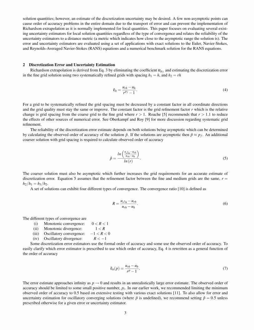
The least squares approach requires at least four solutions. The discretization error and uncertainty estimator, labeled LSQ-09, are subject to different conditions depending on the value of p for p f = 2

ULSQ−09 =

1.25|εLSQ|+Us, 0.95≤ p≤ 2.05min(1.25|εLSQ|+Us,1.25∆M), 0 < p≤ 0.95max(1.25|εLSQ|+Us,1.25∆M), p≥ 2.05∆M, f or all other values

(23)

where εLSQ = αhp1 , Us is the RMS of the fit, and

∆M = max(∣∣ui−u j

∣∣), 1≤ i≤ ng, 1≤ j ≤ ng. (24)

The least squares method was modified in Eca [16] to correct some of the deficiencies in the LSQ-09 method. Thismethod labeled LSQ-10 estimates the discretization uncertainty using two additional error functions based on fixed-exponentpower series expansions. The additional error functions were added to account for cases where the least squares observedorder of accuracy is greater than the formal order ε2

LSQ = αh2k , and where the least squares observed order of accuracy is not

near the formal order of accuracy ε12LSQ = α1hk +α2h2

k . If observed order of accuracy does not fit the above conditions thenε∆M = ∆M/(rpm −1) is used where pm = 1 for p f = 2. Uncertainty estimation for p f = 2 is outlined in Ref. [16] as

ULSQ−10 =

1.25|εLSQ|+Us, 0.95≤ p≤ 2.05min(1.25|εLSQ|+Us,3|ε12

LSQ|+U12s ), 0 < p≤ 0.95

max(1.25|εLSQ|+Us,3|ε2LSQ|+U2

s ), p≥ 2.053|ε∆M |, f or all other values,

(25)

where U12s and U2

s are the RMS of the least squares fit for ε12LSQ and ε2

LSQ, respectively.

3 Analysis3.1 Reliability Metrics

To provide an assessment of the accuracy of the discretization error and uncertainty estimates, the effectivity index [17]for each solution variable is computed as

θL2 =||εh||L2

||εh||L2

. (26)

The discrete L2-norm is computed using

|| f ||L2 =

√1N

N

∑i=1

f 2i (27)

where f is any vector of length N. The L2-norms in this paper are computed for a data set which is composed of a localsolution variable on the computational domain with N grid nodes. The effectivity index should converge to one as the grid isrefined for an accurate error estimate.

6

The primary metric for reliability of the uncertainty estimators is conservativeness where an uncertainty estimate isconsidered conservative if the estimate is greater than the absolute value of the exact error

U > |εh|. (28)

The generally accepted goal of conservativeness for a discretization uncertainty estimator is that 95 percent of all estimatesshould be conservative. To compare how accurately the uncertainty estimate compares to the exact error, an equivalenteffectivity index is computed in a manner similar to the effectivity index for discretization error

ψL2 =||U ||L2

||εh||L2

. (29)

The uncertainty effectivity index is meant to compare how closely the uncertainty estimates bound the exact error. Conserva-tiveness is the most important metric; however, choosing a factor of safety of 1000 may result in a 100 percent conservativeuncertainty estimator but would not provide meaningful information about the uncertainty. The over-estimation of the uncer-tainty would be reflected in the uncertainty effectivity index. As a point of reference, the ideal uncertainty estimator shouldhave a conservativeness greater than 95 percent and an uncertainty effectivity index approaching one as the mesh is refined.

3.2 Distance from the Asymptotic RangeTo assess the reliability of the discretization error and uncertainty estimators suitable for many simulations of varying

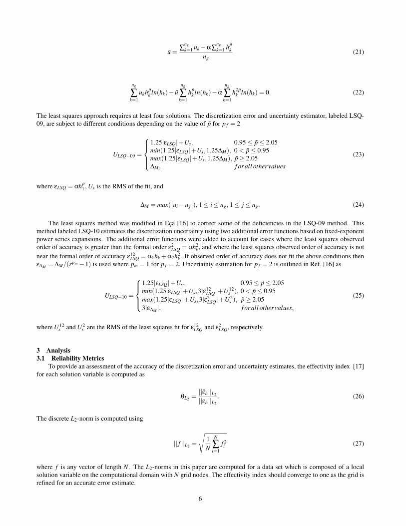
complexity, the reliability metrics should be plotted versus a metric which can be correlated to the confidence in the error oruncertainty estimate. The primary metric for confidence is the observed order of accuracy, where an exact estimate resultswhen p = p f with a high degree of confidence and with degrading confidence as the difference between observed order andformal order increases. This metric is referred to as a distance metric, and ideally, the metric should correlate the reliabilitymetrics for a wide range of problems so that for a given distance from asymptotic convergence the estimates can be said to bereliable. Some possible metrics not based on order of accuracy include cell size or cell count used by Phillips and Roy [11]since these values are commonly used as the absicca for discretization error or order of accuracy plots for a grid convergencestudy. Cell size and cell count are specific only to the set of systematically refined grids for a given application so make apoor choice for correlating reliability metrics for several applications. The correction factor was used as a distance metricby Stern et al. [13] but different refinement factors result in different correction factors making CF a poor choice. Otherpossible distance metrics considered include the global order of accuracy defined in Eq. 13, the FS method parameter P, theglobal deviation from the formal order developed by Phillips and Roy [18], and the percent of monotonically convergingnodes. The FS method parameter P is modified for this study by averaging over the local estimates

P =1N

N

∑i=1

Pi. (30)

The global deviation from the formal order of accuracy computes the average distance from the formal order of accuracyaveraged over the entire domain

∆ p = min

(1N

N

∑i=1

min(∣∣p f − pi

∣∣ ,4p f),0.95p f

). (31)

The observed order of accuracy pi for this distance metric is an empirically modified calculation of the observed order ofaccuracy using absolute values to include the effects of oscillatory converging nodes

p =ln(∣∣∣ ur2h−urh

urh−uh

∣∣∣)ln(r)

. (32)

The percent of Richardson nodes as defined in Section 2.2 was used by Cadafalch et al. [7] as a measure of reliability. Thisdefinition includes monotonically diverging nodes which are not asymptotic, so instead monotonically diverging nodes areexcluded and only the percent of monotonically converging nodes is considered as a distance metric instead. That is thepercentage of all nodes for a given solution variable with a convergence ratio in the range 0 < R < 1.

7

Fig. 1. Comparison of data for two different uncertainty estimators with quadratic fit and bounds for less scatter (top row) and more scatter(bottom row)

3.3 Data representation

The reliability metrics are computed for over 700 data points for six different discretization error estimators and sixdifferent uncertainty estimators. To more clearly present the data, a quadratic regression fit of the reliability metrics versusthe distance metric is computed for each error and uncertainty estimator. The purpose of the regression fit is to capturehow the reliability metrics behave as solutions approach the asymptotic range. Equally important, is how much scatter ispresent in the reliability metrics where more scatter indicates less predicatiblity from application to application and a lessreliable error or uncertainty estimator. To represent the scatter in the data, the 95 percent confidence bound for the quadraticregression fit is computed. The confidence bounds on the regression fit are meant only for comparison purposes to comparethe asymptotic behavior and scatter in the reliability metrics for each error and uncertainty estimator. For the error anduncertainty effectivity index, the regression fit is computed for the inverse effectivity index versus the distance metric. Thisis done because of the range of the data. Several different plotting styles were compared and the inverse of the effectivityindex presented the data best with the most accurate regression fit and confidence bounds. For illustrative purposes only,Fig. 1 shows the raw data for the inverse uncertainty effectivity index and the conservativeness of the uncertainty estimatoralong with the resulting quadratic fit and confidence bounds for two different uncertainty estimators. The distance metricused is the global deviation from the formal order. The inverse uncertainty effectivity index for two different uncertaintyestimators have similar asymptotic behavior but have different amounts of scatter in the data. For conservativeness, only thelower bound is needed because the upper bound is not meaningful. Both the asymptotic behavior and scatter in the data areaccurately represented by the confidence bounds.

4 Applications

Solutions to various applications are computed using three different finite volume solvers with a formal order of accuracyof two. The solvers include an in-house 2D, structured, Euler solver; Loci-Chem, a 3D, unstructured, Reynolds AveragedNavier-Stokes (RANS) solver [19]; and PARNASSOS, a 3D, structured, incompressible RANS solver [20]. All simulationswere performed in double precision and the iterative residuals were converged to machine zero, thus round-off and iterativeerror may be neglected. The finite volume solution is piecewise constant over a cell so the solution is assumed to be locatedat the geometric cell center which is a second-order approximation and a local fourth-order least squares curve-fit is usedto interpolate the cell-centered values to the nodes. The discretization error and uncertainty is estimated at every coincidentnode for a given grid triplet (or grid quadruplet for the LSQ methods) for local solution variables (e.g. density, pressure, andvelocity). A summary of all solutions and grid triplets are given in Table 1.

8

Table 1. Summary of Numerical Solutions

Application Equation Set Variables Grid Triplets Total Estimates

Subsonic MMS Euler ρ, p, u, v 11 44

Supersonic MMS Euler ρ, p, u, v 11 44

Ringleb’s Flow Euler ρ, p, u, v 7 28

Supersonic Vortex Flow Euler ρ, p, u, v 11 44

Loci-Chem MMS RANS BSL-kε ρ, p, u, v, w 4 20

(hexahedral cube RANS BSL-kω ρ, p, u, v, w 4 20

and curvilinear) Euler ρ, p, u, v, w 4 20

NS ρ, p, u, v, w 4 20

NS: Extrapolation BC ρ, p, u, v, w 4 20

NS: Farfield BC ρ, p, u, v, w 4 20

NS: Inflow BC ρ, p, u, v, w 4 20

Loci-Chem MMS RANS BSL-kε ρ, p, u, v, w 4 20

(prismatic cube RANS BSL-kω ρ, p, u, v, w 4 20

and curvilinear) Euler ρ, p, u, v, w 4 20

NS ρ, p, u, v, w 4 20

NS: Extrapolation BC ρ, p, u, v, w 4 20

NS: Farfield BC ρ, p, u, v, w 4 20

NS: Inflow BC ρ, p, u, v, w 4 20

Loci-Chem MMS RANS BSL-kε ρ, p, u, v, w 4 20

(tetrahedral cube RANS BSL-kω ρ, p, u, v, w 4 20

and curvilinear) Euler ρ, p, u, v, w 4 20

NS ρ, p, u, v, w 4 20

NS: Extrapolation BC ρ, p, u, v, w 4 20

NS: Farfield BC ρ, p, u, v, w 4 20

NS: Inflow BC ρ, p, u, v, w 4 20

Loci-Chem MMS RANS BSL-kε ρ, p, u, v, w 4 20

(hybrid cube, RANS BSL-kω ρ, p, u, v, w 3 15

curvilinear, and) Euler ρ, p, u, v, w 4 20

highly curvilinear) NS ρ, p, u, v, w 4 20

NS: Extrapolation BC ρ, p, u, v, w 4 20

NS: Farfield BC ρ, p, u, v, w 4 20

NS: Inflow BC ρ, p, u, v, w 4 20

PARNASSOS MMS (Cartesian) INS BSL-kω p, u, v 6 18

PARNASSOS MMS (stretched) INS BSL-kω p, u, v 6 18

PARNASSOS MMS (non-orthogonal) INS BSL-kω p, u, v 6 18

Turbulent Flat Plate RANS Spalart-Allmaras ρ, p, u, v 2 8

9

4.1 Euler Solver4.1.1 Manufactured Solutions

Two applications include the supersonic and a subsonic manufactured solution used in Ref. [21]. The basic manufacturedsolution function is

f (x,y) = a0 +a1sin(

b1xπ

L+ c1π

)+a2sin

(b2yπ

L+ c2π

)(33)

where the coefficients a, b, c are coefficients to control the magnitude, period, and phase shift of the solution and L isthe reference length of one. The magnitude a0 for density, x-velocity, y-velocity, and pressure are 1.0kg/m3, 800.0m/s,800.0m/s, and 100,000.0Pa for the supersonic manufactured solution and 1.0kg/m3, 70.0m/s, 90.0m/s, and 100,000.0Pafor the subsonic manufactured solution. The periods range from 0.5 and 2.0 for all solution variables.

Two sets of grids for each manufactured solution are also used to investigate the effect of refinement factor on error anduncertainty estimation. The finest grid for the first grid set is 513x513. This grid is successively coarsened by a factor oftwo to create seven grid levels where the coarsest is 17x17. The second set includes the first nine grids in the first set plusan additional set which when combined with the first set results in refinement factors of 4/3 and 3/2 instead of refinementfactors of two and two between the fine and medium and medium and coarse grids, e.g. 513x513, 385x385, and 257x257instead of 513x513, 257x257, and 129x129.

4.1.2 Supersonic Vortex FlowSupersonic vortex flow [22] consists of a flow around a 90 degrees annulus

ρ(r) = ρi

(1+ γ−1

2 M2i

(1− R2

ir2

)) 1γ−1

u(y,r) = yUr , v(x,r) =− xU

r , P = ργ

γ,

Ui = Miργ−1

2i , U = UiRi

r .

(34)

The flow field is defined as a function of variables at the inner radius of the annulus denoted by the subscript i. The innerradius Ri is 2.0m, the outer radius is 3.0m, the inner density ρi is 1.0kg/m3, and the inner Mach number Mi is 2.0. The finestgrid is 513x257 and is successively coarsened by a factor of two to generate a family of grids where the coarsest is 9x5. Asecond intermediate grid set was also created in the same manner as for the manufactured solutions.

4.1.3 Ringleb’s FlowRingleb’s flow is an inviscid flow around a 180 degree turn [23]. The flow can be supersonic, subsonic, or both depending

on the domain chosen. For this study, a supersonic-only region was chosen. Ringleb’s flow is governed by the stream function

ψ =1q

sin(θ) (35)

where θ is the flow angle and q is the normalized velocity. A total of six grids were generated for Ringleb’s flow from thefinest grid of 257x257 using a refinement factor of two to create five grid levels. An intermediate grid set was also created.

4.2 PARNASSOS4.2.1 Manufactured Solutions

A manufactured solution is used from the 2006 and 2008 Lisbon uncertainty analysis workshops [24]. The manufacturedsolution is for the BSL-kω RANS turbulence model

u = er f (η)v = 1

σ√

π

(1− eη2

)Cp = 0.5ln

(2x− x2 +0.25

)ln(4y3−3y2 +1.25

)νt = 0.25(νt)max η4

νe2−η2ν

k = kmaxη2νe1−η2

ν

(36)

10

Fig. 2. PARNASSOS Cartesian, stretched, and non-orthogonal grids

where Cp is the coefficient of pressure, η = σy/x, ην = σνy/x, σ = 4, σν = 2.5σ, kmax = 0.001, (νt)max = 103ν, and ω = k/νt .The manufactured solution is designed to resemble a boundary layer and is computed on three different grid topologies shownin Fig. 2. Each grid topology has 16 grid levels with grids created in increments of 20 (i.e. 101x101, 121x121, . . . , 401x401).The grids are combined to created a total of 6 grid triplets per grid topology with three variables per solution. In total, thereare 54 grid triplets included in the data set with discretization error estimated for x-velocity, y-velocity, and pressure.

4.3 Loci-CHEM4.3.1 Manufactured Solutions

Several manufactured solutions are used to compute 3D, steady-state solutions to the Euler, Navier-Stokes, and RANSequations with two-equation turbulence models. The manufactured solutions used for code verification of Loci-CHEM arediscussed in [25, 26]. The manufactured solutions include one Euler solution, BSL-kω and BSL-kε RANS solutions, andfour Navier-Stokes solutions which include extrapolation, farfield, and inflow boundary conditions. Three different gridtopologies are used with two different levels of complexity. These grid topologies include hexahedral, tetrahedral, andprismatic grid cells plus a hybrid combination of each on a Cartesian domain, a curvilinear domain, and a highly skewedcurvilinear domain [26]. A few examples are shown in Fig. 3. The grid sizes are 65x65x65, 33x33x33, 17x17x17, and9x9x9. There are a total of two grid triplets per grid topology for seven manufactured solutions with 5 solution variableseach for a total of 555 grid triplets.

Fig. 3. Samples of the Loci-CHEM computational grids showing the (a) Cartesian tetrahedral grid, (b) curvilinear prismatic grid, (c) highlyskewed curvilinear hexahedral grid, and (d) the curvilinear hybrid grid

4.3.2 Turbulent Flat PlateA numerical benchmark solution computed for a zero pressure gradient, turbulent flat plate for the RANS equations

computed using the Spalart-Allmaras turbulence model [27] is used to evaluate the error and uncertainty estimators in placeof an exact solution. The flat plate has a non-dimensional length L of 2 and the Reynolds number at L = 1 is 5,000,000. The

11

Fig. 4. Turbulent flat plate setup and the 69x49 grid

domain and boundary conditions are shown in Fig. 4. The finest grid used for error and uncertainty estimation is 545x385and is successively coarsened by a factor of two to create a total of five grids. A numerical benchmark was created by Phillipset al. [21] using the same computational domain and grid topology as the grids used for error and uncertainty estimation.The numerical benchmark grid dimensions are 2177x1537 nodes and computed using Loci-CHEM. The benchmark solutionwas created using the guidelines included in Phillips et al. [21] which require for a benchmark solution that (1) the numericalbenchmark has been shown to be in the asymptotic convergence range and (2) that the code used to generate the benchmarksolution has passed all order of accuracy code verification tests for all options exercised in the benchmark problem. Bothof these conditions were satisfied for the numerical benchmark and documented by Phillips et al. [21]. The numericalbenchmark was developed with the purpose of evaluating discretization error and uncertainty estimates. The error due tothe presence of discretization error in the benchmark solution is estimated by propagating the estimated discretization errorin the numerical benchmark through the discretization error estimate calculations discussed in this paper. The error in erroreffectivity index computed using Richardson extrapolation with the formal order of accuracy is about 0.1. The numericalbenchmark discretization error has negligible effect on all other computational grids coarser than the 545x385 grid.

5 Results5.1 Distance Metric

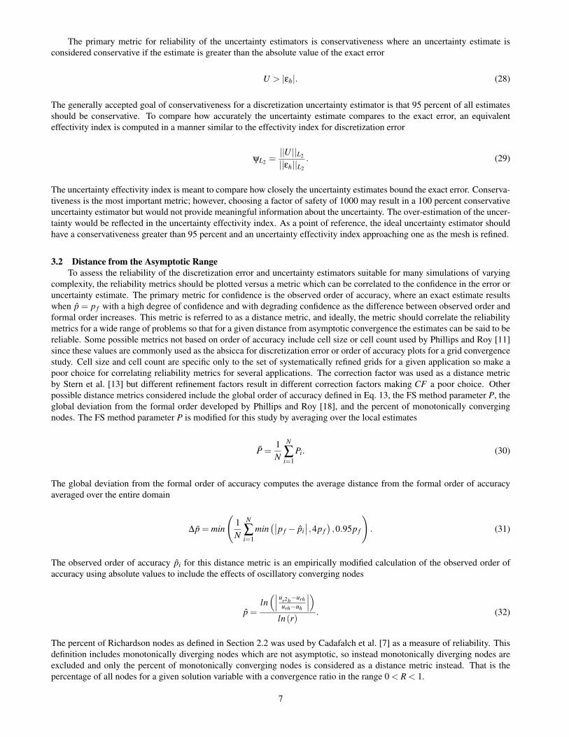
The global observed order of accuracy, the FS method distance metric, global deviation from the formal order, andpercent of monotonically converging nodes are compared in Fig. 5. The error effectivity index for Richardson extrapolationusing the formal order of accuracy (Eq. 4) for all local solution variables in the test data set is plotted for each distancemetric.

The effectivity index should approach one as the solutions become more asymptotic. For the four distance metricsconsidered, an asymptotic solution occurs at zero for the global deviation from the formal order, 100 percent for the percentof monotonically converging nodes, the formal order of accuracy (two for all cases) for the global order of accuracy, andP = 1 for the Factor of Safety method parameter. The ideal distance metric should show decreasing scatter in the datacentered about an inverse effectivity index of one as the data approaches the asymptotic range. Shown in Fig. 5, the globaldeviation from the formal order, percent of monotonically converging nodes, and the global order of accuracy resemble tovarying degrees the expected trend. The distance metric P does not show a clear trend. This is because pFS is not limited toa maximum of p f , and results in the average of P roughly clustering around P = 1. Of the three other distance metrics thathave the particular trend sought, the global deviation from the formal order shows the clearest trend in inverse effectivityindex with significantly reduced scatter as the distance metric approaches zero and no scatter at ∆ p = 0 which is preferred.The percent of monotonically converging nodes and global order of accuracy still have some scatter at asymptotic solutionconvergence (i.e. 100 percent monotonically converging nodes and pglb = p f ). The reason that the global deviation fromthe formal order performs the best is because orders of accuracy greater than one and less than one are treated as equally farfrom the asymptotic range. This treatment is prefered since observed orders of accuracy greater than the formal order andless than the formal order are equally non-asymptotic. The difference is that the signs of the higher order terms allow forerror cancelation or error addition. For an observed order of accuracy greater than the formal order, the first two terms of thehigher order terms will tend to have the same sign, and for orders of accuracy lower than the formal order, the first two termswill tend to have the opposite signs. The percent of monotonically converging nodes is good but not the best choice becauseobserved orders of accuracy greater than the formal order are considerably non-asymptotic but are counted as asymptoticallowing for a misleading more asymptotic distance metric. In a similar manner, the calculation of the global observed orderlimits orders of accuracy greater than the formal order to equal the formal order. This again allows for a misleading moreasymptotic distance metric. Comparison of the distance metric with the uncertainty effectivity index and conservativenessshowed similar trends.

12

Fig. 5. Comparison of the effectivity index for Richardson extrapolation versus various distance measures

5.2 Discretization Error EstimatesDiscretization error estimators are compared in Fig. 6 comparing Richardson extrapolation using a) the formal order of

accuracy, b) the observed order of accuracy, c) observed order of accuracy modifications pOR, d) globally averaged observedorder of accuracy, e) observed order of accuracy modifications pCF , f) and the discretization error estimator proposed byXing and Stern [8]. The least-square fit confidence bounds, computed as described in Section 3.3, for all seven applicationsare compared for a total of about 1.6 million error estimates combined into a total of 777 error effectivity index data points.The use of Richardson extrapolation using the formal order of accuracy is the most accurate error estimator where the datais symmetric about an inverse effectivity index of one for the full range of ∆p. The scatter in the data decreases resultingin more reliable discretization error estimates as solutions approach the asymptotic range (i.e. as ∆p approaches zero). Theother five error estimators use an observed order of accuracy which results in an overestimate of the discretization error dueto the observed order of accuracy factor of safety. The observed order factor of safety refers to the implicit factor of safetydue to the use of the observed order of accuracy εh(p) = FSpεh(p f ) where FSp = rp f −1

rp−1 . (Note that FSp is the inverse ofCF .) The use of the different orders of accuracy results in varying differences in the inverse effectivity index. There arenegligible differences between error estimates which use p, pOR, and pCF . The use of pglb results in slightly more accurateerror estimates compared to εh(p) as well as reduced scatter. The reduced scatter is due to use of a single value of orderof accuracy and observed order factor of safety instead of point-wise variations in the observed order. No error estimatorwas given for the CF method; however, Richardson extrapolation using the observed order of accuracy pCF is included tocompare the effects of not limiting the observed order of accuracy to the formal order. There is no noticable differencebetween limiting the observed order to the formal order or not limiting the observed order. The same order of accuracy isused for the FS method as the CF method; however, the use of P compensates for the underestimate of discretization errorwhen pFS > p f and the overestimate of discretization error when pFS < p f . The use of P results in more accurate errorestimates compared to εh(p) and is the second most accurate error estimator compared.

5.3 Discretization Uncertainty EstimationThe inverse uncertainty effectivity index and the conservativeness are shown in Fig. 7 for the discretization uncertainty

estimators. The inverse uncertainty effectivity index for the GCI-2g method is the same as the error effectivity index forεh(p f ) (Fig. 6a), except that it is shifted by a factor of a third due to the presence of the factor of safety (FS = 3). Similarly,the other uncertainty estimators also approach their inverse factor of safety as p→ p f . The use of the observed order ofaccuracy results in a similar trend as the discretization error estimators which overestimate the uncertainty for non-asymptoticsolutions. The GCI-OR, CF, and FS method all have nearly identical observed orders of accuracy. The differences in thesemethods is due almost exclusively to the choice of factor of safety. The most conservative uncertainty estimators are theLSQ methods which are very similar; however, the uncertainty effectivity index for the LSQ-10 method is significantlyimproved over the LSQ-09 method and results in a much more accurate uncertainty estimate. The LSQ-10 uncertaintyestimator still overestimates the uncertainty considerably more than any of the other uncertainty estimators except the LSQ-

13

Fig. 6. Error effectivity indices for discretization error estimators

Fig. 7. Uncertainty effectivity index and conservativeness for discretization uncertainty estimators

09. The FS, GCI-OR, and GCI-2g uncertainty estimators are the next most conservative estimators. The FS and GCI-ORmethods have very similar trends regarding the uncertainty effectivity index but the FS method is slightly more conservative.The GCI-2g uncertainty estimator is less conservative than both the FS and GCI-OR methods and the uncertainty is alsooverestimated for more asymptotic solutions. The variable factor of safety used both by the FS and GCI-OR method offer anadvantage over a constant factor of safety of three at the cost of one additional solution. The next best uncertainty estimatoris the GCI-glb method which does not compare well to the conservativeness goal of 95 percent for solutions far from theasymptotic range. The poor performance of the method is due primarily to the use of a constant factor of safety of 1.25 whereincreasing the factor of safety would significantly improve performance. It is important to note that the use of the globalobserved order of accuracy compared to the local observed order of accuracy for the same constant factor of safety improvesthe conservativeness for non-asymptotic solutions and results in an uncertainty effectivity index closer to one (results notshown). The use of a global observed order of accuracy could be used with any of the other uncertainty estimators to likewiseimprove both the accuracy and conservativeness. The uncertainty estimator which performs the worst for conservativenessis the CF method; however, the CF method has an uncertainty effectivity index closest to one as ∆p approaches zero.

To add an additional level of comparison between the conservativeness of each uncertainty estimator, the overall con-servativeness is computed for every uncertainty estimate included in the study for approximately 1.6 million estimates andis independent of the distance measure. The results are shown in Table 2 and are sorted from the highest conservativeness tothe lowest. The conservativeness of the absolute value of Richardson extrapolation using the formal order of accuracy is also

14

Table 2. Overall conservativeness of each uncertainty estimator

Estimator All Data p > 0.5 only

# Data 1.6 Million 1.3 Million

LSQ-09 97.7% −

FS 97.5% 97.4%

LSQ-10 97.0% −

GCI-OR 95.8% 95.3%

GCI-2g 95.2% 97.0%

GCI-glb 92.6% 92.4%

CF 89.7% 90.3%

|εh(p f )| 49.8% 52.4%

included for comparison and is expected to be 50 percent as discussed by Roache [5] and Oberkampf and Roy [9]. The LSQ,FS, GCI-OR, and GCI-2g methods all meet the 95 percent conservativeness goal. To show the effects of the modificationsto the observed order of accuracy (setting oscillatory nodes to 0.5 and limiting orders of accuracy to a minimum of 0.5) thatwere implemented to estimate the uncertainty at diverging and oscillatory nodes, the uncertainty estimators were applied toonly the data with p > 0.5. This represents about 83 percent of all the data. The FS, GCI-OR, and GCI-glb methods showa very slight decrease in conservativeness and the CF method shows a very slight increase in conservativeness. The mostsignificant change is in the GCI-2g method which had an increased conservativeness of almost two percent points makingit one of the better performers with 97 percent conservativeness. The lack of change between including and excluding thespecific data supports our modifications to the uncertainty estimators for oscillatory nodes. Furthermore, it also supportsour hypothesis that local solutions are, in practice, non-asymptotic and uncertainty estimates for monotonically convergingnodes are as reliable as diverging, oscillatory converging or oscillatory diverging nodes.

The CF method was the only uncertainty estimator other than the LSQ methods which specified treatment for oscillatorynodes given in Eq. 17. All other GCI methods were modified for this study to assign a value of 0.5 to the order of accuracy ofoscillatory nodes to compute an uncertainty estimate. The lower limit of 0.5 was applied to the CF method to compare the twodifferent treatments of oscillatory nodes. The resulting overall conservativeness for the CF method was 91.5 percent whichis only a slight increase in percent over Eq. 17. There was little change in the overall trends of the uncertainty effectivityindex.

6 ConclusionRichardson extrapolation-based discretization error and uncertainty estimators were applied to several different appli-

cations with a focus on uncertainty estimation for local solution quantities. The estimators were applied to all coincidentgrid nodes including diverging and oscillating nodes. All nodes were included to thoroughly investigate the behavior ofeach estimator because it is not always possible to have local solutions in the asymptotic range; however, a conservativeestimate of discretization uncertainty is still desirable, and as demonstrated herein, is possible. The reliability of the errorand uncertainty estimates was quantified using the error effectivity index, the uncertainty effectivity index, and the overallconservativeness of the uncertainty estimates. The global deviation from the formal order of accuracy was the distance mea-sure used to correlate the effectivity indices and conservativeness. A total of 777 grid triplets and a total of 1.6 million localestimates were examined.

Overall there was a general trade-off between the accuracy of the error and uncertainty estimates and the conservative-ness. The most accurate uncertainty estimator (e.g. effectivity index closest to one) was the CF method but it was also theleast conservative. The LSQ methods were the most conservative but significantly overestimated the uncertainty comparedto the other methods. The LSQ-10 was much more accurate than the LSQ-09 method with nearly identical conservativenessand should be used instead of the LSQ-09 method. The LSQ-10 and the FS method were very similar in terms of conser-vativeness. The LSQ-10 method was more conservative for less asymptotic solutions but the overall conservativeness of theFS method was 0.5 percent better. The FS method was more accurate than the LSQ-10 with an uncertainty effectivity indexcloser to one and had significantly less scatter in the metrics. The LSQ and the FS methods perform similarly and eithercould be applied successfully for accurate uncertainty estimation; however, the FS method requires only three solutions andis easier to implement than the LSQ methods which require at least four solutions. If only two solutions are available, theGCI-2g method should be used as the overall conservativeness met the 95 percent conservativeness goal for this data set and

15

has been reliably applied to a wide range of applications.It was also observed that the use of a global order of accuracy improved the conservativeness and accuracy of the

uncertainty estimator and decreased the scatter in the data in the effectivity index. While the GCI-glb did not perform wellcompared to the other uncertainty estimators due to the constant factor of safety of 1.25, the use of a global order of accuracyfor local estimates would improve the overall performance of the other uncertainty estimators considered.

The uncertainty estimators were evaluated using simple Euler and Navier-Stokes solutions which are relatively easy toreach the asymptotic range. The uncertainty estimators should be evaluated further using more realistic problems; however,the lack of exact solutions makes the evaluation of the uncertainty estimators more ambiguous and is a current topic ofresearch.

References[1] Banks, J. W., Aslam, T., and Rider, W. J., 2008. “On sub-linear convergence for linearly degenerate waves in capturing

schemes”. Journal of Computational Physics.[2] Roache, P. J., 1994. “Perspective: A method of uniform reporting of grid refinement studies”. J of Fluid Eng, 116(3),

pp. 405–413.[3] Celik, I. B., Ghia, U., Roache, P. J., Freitas, C. J., Coleman, H. W., and Raad, P. E., 2008. “Procedure for estimation

and reporting of uncertainty due to discretization in cfd applications”. J of Fluid Eng, 130(7), pp. 78001–78005.[4] Cosner, R. R., Oberkampf, W. L., Rumsey, C. L., Rahaim, C. P., and Shih, T. I.-P., 2006. AIAA committee on standards

for computational fluid dynamics: Status and plans. AIAA-2006-889.[5] Roache, P. J., 2009. Fundamentals of Verification and Validation. Hermosa Publishers, Albuquerque, NM.[6] Logan, R. W., and Nitta, C. K., 2006. “Comparing 10 methods for solution verification, and linking to model valida-

tion”. JACIC, 3, pp. 354–373.[7] Cadafalch, J., Perez-Segarra, C. D., Consul, R., and Oliva, A., 2002. “Verification of finite volume computations on

steady-state fluid flow and heat transfer”. J Fluid Eng, 124(1), pp. 11–21.[8] Xing, T., and Stern, F., 2010. “Factors of safety for richardson extrapolation”. J Fluid Eng, 132(6), p. 61403.[9] Oberkampf, W. L., and Roy, C. J., 2010. Verification and Validation in Scientific Computing. Cambridge University

Press Cambridge.[10] Stern, F., Wilson, R. V., Coleman, H. W., and Paterson, E. G., 2001. “Comprehensive approach to verification and

validation of cfd simulations - part 1: Methodology and procedures”. J Fluid Eng, 126(4), pp. 793–802.[11] Phillps, T. S., Derlaga, J. M., and Roy, C. J., 2012. “Numerical benchmark solutions for laminar and turbulent flows”.

AIAA-2012-3074.[12] Roache, P. J., 2003. Error bars for cfd. AIAA-2003-408.[13] Wilson, R., Shao, J., and Stern, F., 2004. “Discussion: Criticisms of the correction factor verification method”. J Fluid

Eng, 126(4), pp. 704–706.[14] Eca, L., and Hoekstra, M., 2002. An evaluation of verification procedures for cfd applications. 24th Symposium on

Naval Hydrodynamics, Fukuoka, Japan, July 8-13.[15] Eca, L., and Hoekstra, M., 2009. “Evaluation of numerical error estimation based on grid refinement studies with the

method of the manufactured solutions”. Computers and Fluids, 38(8), pp. 1580–1591.[16] Eca, L., 2010. Uncertainty quantification for cfd. Personal communication.[17] Ainsworth, M., and Oden, J. T., 2000. A Posteriori Error Estimation in Finite Element Analysis. Wiley, New York.[18] Phillips, T. S., and Roy, C. J., 2013. “A new extrapolation-based uncertainty estimator for computational fluid dynam-

ics”. AIAA-2013-0260.[19] Luke, E. A., Tong, X., Wu, J., and Cinnella, P., 2010. Chem 3.2: A finite-rate viscous chemistry solver – the user guide.

Tetra Research Corporation.[20] Hoekstra, M., and Eca, L., 1998. Parnassos: An efficient method for ship stern flow calculation. Proc. 3rd Osaka

Colloquium, Osaka, Japan, pp. 331-357.[21] Phillps, T. S., and Roy, C. J., 2011. “Residual methods for discretization error estimation”. AIAA-2011-3870.[22] Ollivier-Gooch, C., Nejat, A., and Michalak, K., 2009. “Obtaining and verifying high-order unstructured finite volume

solutions to the euler equations”. AIAA Journal, 47(4), pp. 2105–2120.[23] Satav, V., Hixon, R., Nallasamy, M., and Sawyer, S., 2005. “Validation of a computational aeroacoustics code for

nonlinear flow about complex geometries using ringleb’s flow”. AIAA-2005-2871.[24] Eca, L., and Hoekstra, M., 2005. Workshops on cfd uncertainty analysis. Maretec, http://maretec.inst.utl.pt.[25] Veluri, S. P., 2010. “Code verification and numerical accuracy assessment for finite volume cfd codes”. PhD thesis,

Virginia Tech.[26] Veluri, S. P., Roy, C. J., and Luke, E. A., 2012. “Comprehensive code verification techniques for finite volume cfd

codes”. Comput Fluids, 70(30), pp. 59–72.

16

[27] Rumsey, C. L., Smith, B. R., and Huang, G. P., 2010. “Description of a website resource for turbulence modeling,verification and validation”. AIAA-2010-4742.

17