Revisiting Random Walk Hypothesis in Indian Stock Market-An Empirical Study on Bombay Stock Exchange

Swapan Sarkar Assistant Professor of Commerce

Harimohan Ghose College, Kolkata e-mail : swapansarkar22@gmail.com

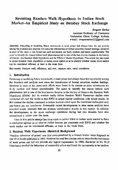
Abstract: Predicting or modeling future movements in asset prices had always been the top priority among the investors and analysts ever since the introduction offonnal securities market dealings. However in most of the cases it was found that such movements are fairly random and hence unpredictable. The quest to identify the reason behind such phenomenon led to two of the best known theories in the history of finance - the Random Walk Hypothesis and the Efficient Market Hypothesis. This article has attempted to revisit Random Walk Hypothesis in Indian stock market so as to identify whether Indian stock mark.et can be considered efficient, at least in the weak fonn.

Key-words: Random walk, efficiency, unit root, variance ratio, serial correlation.

1- Introduction Predicting or modeling future movements in asset prices had always been the top priority among the investors and analysts ever since the introduction of formal securities market dealings. However in most of the cases such efforts were found to be useless as price movements are fairly random and hence unpredictable. The quest to identify the reason behind such phenomenon Jed to one of the best known theories in the history of finance-the Random Walk Hypothesis (RWH). But do markets really follow Random Walk? Numerous studies were

conducted all over the world to test RWH in actual market conditions with mixed results. In this context the studies conducted in Indian bourses relied upon the traditional techniques only and hence are not conclusive. Fortunately recent developments in time series analysis have provided ample measures that can produce corroborative results in this respect. In addition the developments in the stock exchange operations during last two decades have also necessitated a relook over the issue.

Thus in this article attempt has been made to revisit RWH in Indian stock market to form a conclusive opinion as to whether Indian bourses are consistent with RWH and whether the stock market can be considered efficient, at least in the weak form.

2- Random Walk Hypothesis; Historical Background 'Random behaviour of prices' was first conceptuali7.ed by a French broker Jules Regnault in one of his books published in 1863. However he used the concept only to describe the movement of stock prices and did not provide any logical explanation. In 1900, Bachelier in his Ph.D dissertation studied the behaviour of commodity prices and found the movements to be random.

55

Business Studiu-Vol: XXXV & XXXVI, 2014 & 2015

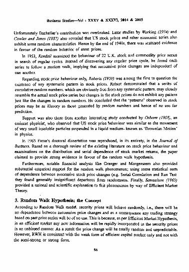
Unfortunately Bachelier's contribution was overlooked. Later studies by Working (1934) and Cowles and Jones (1937) also revealed that US stock prices and other economic series also exhibit some random characteristics. Hence by the end of 1940s, there was scattered evidence in favour of the random behavior of asset prices.

In 1953, Kendall examined the behaviour of 22 U.K. stock and commodity price series in search of regular cycles. Instead of discovering any regular price cycle, he found each series to follow a random walk, implying that successive price changes are independent of

one another.

Regarding stock price behaviour only, Roberts (1959) was among the first to question the existence of any systematic pattern in stock prices. Robert demonstrated that a series of cumulative random numbers, which are obviously free from any systematic pattern, may closely resemble the actual stock price series but changes in the stock prices do not exhibit any pattern just like the changes in random numbers. He concluded that the 'patterns' observed in stock prices may be as illusory as those generated by random numbers and hence of no use for prediction.

Support was also there from another interesting study conducted by Osborn (1959), an eminent physicist, who observed that US stock price behaviour was similar to the movement of very small insoluble particles suspended in a liquid medium- known as 'Brownian Motion' in physics.

In 1965 Fama's doctoral dissertation was reproduced, in its entirety, in the Journal of Business. Based on a thorough review of the existing literature on stock price behaviour and examinations on the distribution and serial dependence of stock market returns, the paper claimed to provide strong evidence in favour of the random walk hypothesis.

Furthermore, notable financial analysts like Granger and Morgenstern also provided substantial empirical support for the random walk phenomenon; using some statistical tests of dependence between successive stock price changes ( e.g. Serial Correlation and Run Test they found generally insignificant departures from randomness. Finally, Samuelson (1965) provided a rational and scientific explanation to this phenomenon by way of Efficient Market Theory.

3. Random Walk Hypothesis; the Concept

According to Random Walk model, security prices will behave randomly, i.e., there will be no dependence between successive price changes and as a consequence any trading strategy based on past price series will be of no use. This is because, as per Efficient Market Hypothesis, in an efficient market any new information will be rapidly incorporated in the security prices in an unbiased manner. As a result the price change will be totally random and unpredictable. However, RWH is consistent with the weak form of efficient capital market only and not with the semi-strong or strong form.

56

Swapan Sarkar

4. Literature Review Studies in International Context

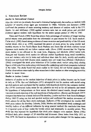
After the initial era (as already discussed in historical background), the studies on random walk behavior of security prices again got momentum in 1980s. Porterba and Summers (1988) confirmed the presence of mean reverting tendency and absence of random walk in the U.S. Stocks. Lo and McKinney (1988) applied variance ratio test on stock prices and provided evidence against random walk hypothesis for the entire sample period of I 962 to 1985.

Fama and French (1988) found that almost forty percentage of variation of longer holding period returns were predictable from the information on past returns for U.S. Stock markets. Culler et al. (1990) found strong evidence of mean reversion and predictability of the US stock market return. Kim et at. (1991) examined the pattern of stock prices by using weekly and monthly returns in five Pacific-Basin Stock Markets and found that all stock markets except Japanese stock market did not follow random walk. Olowe (1999) showed that the Nigerian stock market is not efficient in the weak form. Shiguang and Michelle (2001) tested both Shanghai and Shenzen stock market for efficient market hypothesis using serial correlation, runs and variance ratio test to index and individual share data for daily, weekly and monthly frequencies and found that Chinese stock markets were not weak form efficient. Chakraborty (2006) investigated the stock price behaviour of Sri Lankan stock market using daily closing figures ofMilanka Price Index along with twenty-five underlying individual companies included in the index. The study found that stock market in Sri Lanka did not follow random walk. Similar observations were made by other researchers in their studies on other emerging securities market in recent times.

Studies in Indian Context

Instances of studies on the random behaviour of stock prices in Indian bourses can be found as early as 1970s. Rao and Mukherjee (1971) attempted to test the random walk model using spectral analysis and concluded that the random walk hypothesis held for the company studied. Ray (1976) constructed index series for six industries as well as for all industries and tested the hypothesis of independence on these series. He obtained mixed results, though evidence was more towards rejection of the null hypothesis of independence. Sharma and Kennedy (1977) compared the behaviour of stock indices of the Bombay, London and New York Stock Exchanges during 1963-73 using run test and spectral analysis and confirmed the random movement of stock indices for all the three stock exchanges. Kulkarni (1978) investigated the weekly RBI stock price indices for Bombay, Calcutta, Delhi, Madras and Ahmedabad stock exchanges and monthly indices of six different industries by using spectral method. He concluded that there is a repeated cycle of four weeks for weekly prices and seasonality in monthly prices. This study has thus rejected the hypothesis that stock price changes were random. Barua (1981) analyzed daily price changes of 20 securities and Economic nmes index from July 1977 to June 1979. He found no dependence in individual security price changes but the market index

57

Business Studie,._Vol : XXXV & XXXVI, 2014 & 2015

exhibited significant serial dependence. Sharma (1983) analyzed weekly returns of 23 actively traded stocks in BSE over the period 1973-78. The integrated moving average from the random walk model was fitted on the series and was found to be an adequate representation of price changes except for two stocks. These are the stocks for which no adjustment was made for rights and bonus issues. In a more comprehensive study, Gupta (1985) tested random walk hypothesis using daily and weekly share prices of 39 shares together with the Economic Times and Financial Express indices of share prices. He concluded that the Indian stock markets might be termed as competitive and 'weakly' efficient in pricing shares. Ramachandran (1985) tested weekend prices of 60 stocks covering the period 1976-81 for the weak form of EMH. He used filter rule tests in addition to runs and serial correlation tests and found support for the:weak form of EMH. In a more recent study Rao (1988) examined weekend price data over the period July I 982 to June 1987 for ten blue chip companies by means of serial correlation analysis, runs tests and tilter rules only to confirm the weak form of efficiency. Yalawar (1988) studied the monthly closing prices of 122 stocks listed on the Bombay Stock Exchange during the period I 963-82. He used Spearman 's rank correlation test and runs test and found that only 21 out of 122 lag I correlation coefficients were significant at 5% level thereby supporting the weak form efficiency. Obeidul/ah (1991) used weekly prices covering the period 1985-88 and examined serial correlation and runs. He found significant support for the weak form of EMH.

Poshakwa/e (1996) studied the daily prices of BSE National Index for the period 1987-94 to test existence of day of the week effect in BSE. He used K-S Goodness of Fit test, serial correlation test and run test and found that weekend effect is evident thus rejecting any possibility of weak form efficiency. Pandey (2003) in his study on NSE indices used the daily and weekly values of three leading indices namely CNX DEFTY, CNX NIFTY and CNX NIFTY JUNIOR for the period 1996-2002. He performed autocorrelation analyses and runs test and concluded that the series of stock indices in the India Stock Market are biased random time series. In a more recent attempt, Srinivasan (2010) studied the daily closing values of CNX NIFTY and the BSE SENSEX for the period 1st July 1997 to 31st August 2010 using more advanced test techniques like ADF test and PP test. The results confirmed that the return series does not contain any unit root and hence the market is not efficient in the weak form. Mishra (2010) also confirmed the same results on both BSE and NSE as documented by Srinivasan (2010).

5. Objective of the Study

As evident from the discussion in the literature review section, while the studies on foreign stock exchanges always relied upon advance test techniques, the studies conducted on Indian bourses used mostly the traditional test techniques ( except in a few recent cases). Therefore, the general belief that Indian bourses do satisfy the RWH and accordingly are efficient in weak form is quite doubtful. Moreover the recent development measures by stock exchanges and

58

Swapan Sarkar

capital market regulator, i.e., SEBI have also changed the scenario a lot. Hence the primary objective of the study will be

• To reassess the validity of RWH in Indian stock market with a special reference to the Bombay Stock Exchange (BSE) by applying advanced statistical techniques in addition to the traditional techniques,

against the secondary objective to justify the weak form efficiency of BSE and of Indian Stock market.

6. Sample and Data To achieve the stated objective, this study has considered four major indices of Bombay Stock Exchange namely BSE 30 (popularly known as SENSEX), BSE 100, BSE 200 and BSE 500.

The four indices are selected because of their popularity and extensive use as benchmark to represent mid-cap, small-cap and large-cap companies by most of the mutual funds and industry experts.

The period of the study has been taken to be the period starting from 01.04.2005 up to 31.03.2015 for each index.

Daily closing index values were collected for each of the four indices for the above specified period to calculate the daily returns on each index. The data-source used for this purpose is the official website of BSE.

The return is calculated as the logarithmic difference between two consecutive prices in a series, yielding continuously compounded returns. The reasons to take logarithm returns are justified by both theoretically and empirically.

Theoretically, logarithmic returns are analytically more tractable. On the other hand, empirically logarithmic returns are more likely to be normally distributed which is a prior condition of many standard statistical tests employed in analyzing financial time series. Daily index returns (R,) are calculated as:

R1 = Ln (11 / 11_1 ), Where, R1 = return at period t; 11 = Index value at the end of period t.

Statistical tests are applied on th., return series calculated as above.

7. Methodology The study has considered a few advanced test techniques less familiar in this kind of studies conducted on Indian bourses, along with the popular and well known techniques. The popular list includes Serial or Auto Correlation Test and Run Test whereas the advanced techniques include Ljung-Box (Q) Statistic, Unit Root tests and Variance Ratio test. These are discussed below.

SeriaVAuto Correlation Test

Serial correlation (also called Auto-correlation) measures the correlation between price changes in consecutive time periods. Hence, a serial correlation that is positive and statistically

59

Business Studies-Vol : XXXV & XXXVI, 2014 & 2015

significant could be viewed as an evidence of price momentum in markets and would suggest that returns in a period are more likely to be positive (negative) if the prior period's returns were positive (negative). Similarly a negative serial correlation, which is statistically significant, could be an evidence of price reversal. But if the serial correlation is found to be zero or statistically insignificant, it will confirm independence of successive price changes which is the

pre condition for a random walk.

Serial/Auto correlation function for the series Y, is measured by the following formula:

. . rf-k+t (Y, - Y) (Y,-k - Y) Auto-correlationatlagk,1.e., ACF(k) = rf=tCY, -Y)2

mean ofY and n = length of the series.

The standard error of ACF (k) is given by:

1 SeACF(k) = _ r:::--;:

vn-k When n is sufficiently large, i.e., n .? 50, it is reduced to

1 SeACF(k) = yn

where y = sample

To test whether ACF (k) is significantly different from zero, t statistic is calculated as:

ACF(k) t=---

SeACF(k)

If t statistic is found to be significant, it confirms independence of successive price changes and hence random walk of return series.

Ljung-Box (Q) Statistic

Ljung-Box portmanteau statistic (Q) is used to test the joint hypothesis that all

autocorrelations up to a certain lag are simultaneously equal to zero. The Ljung-Box Q

m •2

statistic is given by: Q* = T(T + 2) '\' ...!..!_-x;. where T =no.of observations LT-k k=l

and ,k= k-th autocorrelation.

Under the null hypothesis of zero autocorrelation at the first m autocorrelations, the Ljung­Box Q-statistic is also distributed as Chi-squared with degrees of freedom equal to the number

of autocorrelations (m). Existence of significant Q statistic is a clear indication of the series being non-random with successive changes being non-independent.

60

Swapan Sarkar

Run Test

Though Serial Correlation based test techniques are quite useful, it requires a basic assumption that the series follows normal distribution. Hence for any series which does not follow normal distribution, the serial correlation test results cannot be conclusive. Here arises the importance of Run Test which is a non-parametric test in which the number of sequences of consecutive positive and negative returns is tabulated and compared against its sampling distribution under the random walk hypothesis. A run is defined as the repeated occurrence of the same value or category of a variable. Stock price runs can be positive, negative, or have no change. The length is how often a run type occurs in succession. Under the null hypothesis that successive outcomes are independent, the total expected number of runs is distributed as normal with

the following mean (µ) and S.D. ( cr):

N(N + 1) - tf=t nf µ= N

_ tf=1[If=1 nf + N(N + 1)] - 2N(If=1 nf - N3 ) 112 cr - [ N 2(N - 1) ]

Where n, is the number of runs of type i and N stands for total number of price changes. The test for serial dependence is carried out by comparing the actual number of runs, a, in the return series,

to the expected number µ. The resultant z statistic is:

Z= ar-µ (J

If the Z statistic is found to be insignificant, random walk of the return series is confirmed.

Unit Root Tests

These tests are used to identify whether a given time series is non-stationary or not. A series is said to be non-stationary if it has a time varying (i.e. dependent on time) mean or time varying variance or both. By contrast, a weak stationary time series has both its mean and variance constant over time. Such a time series will tend to return to its mean (mean reversion) and fluctuations around the mean will have broadly constant amplitude:

A Random Walk Model is necessarily a non-stationary process. However, there are three different forms of random walk.

(i) Pure Random Walk: A pure random walk is defined as Y, = Y ., + u, where the value ofY at time t is equal to its previous value and a random shock. This is also known as random walk without drift (or without intercept). Since E(u,) = 0, E(Y,) = Y0 and V(Y,) = tcr1, i.e., a pure random walk has a constant mean but its variance is dependent on time. Thus a pure random walk is a non-stationary process.

61

Business Studiet-Vol : XXXV & XXXVI, 2014 & 2015

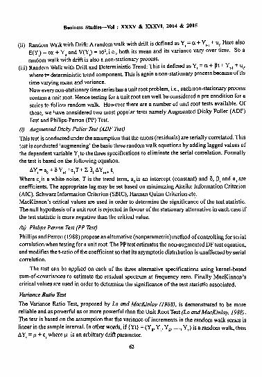
(ii) Random Walk with Drift: A random walk with drift is defined as Y, = OL + Y,_1 + u,. Here also E(Y,) = tOL + y O and V(Y,) = to', i.e., both its mean and its variance vary over time. So a random walk with drift is also a non-stationary process.

(iii) Random Walk with Drift and Deterministic Trend: This is defined as Y, = OL + ~t + Y,_, + u,, where t= deterministic trend component. This is again a non-stationary process because of its time varying mean and variance. Now every non-stationary time series has a unit root problem, i.e., each non-stationary process contain a unit root. Hence testing for a unit root can well be considered a pre condition for a series to follow random walk. However there are a number of unit root tests available. Of these, we have considered two most popular tests namely Augmented Dicky Fuller (ADF) Test and Philips-Perron (PP) Test.

(i) Augmented Dicky Fuller Test (ADF Test)

This test is conducted under the assumption that the errors (residuals) are serially correlated. This test is conducted 'augmenting' the basic three random walk equations by adding lagged values of the dependent variable Y, to the three specifications to eliminate the serial correlation. Formally the test is based on the following equation.

liY,= a,+ 6 Y,_1 +a,T+ :E ~; liY,.;+ £, Where £,is a white noise, Tis the trend term, a0 is an intercept (constant) and 6, ~; and a, are coefficients. The appropriate lag may be set based on minimizing Akaike Information Criterion (AIC), Schwarz Information Criterion (SBIC), Hannan Quinn Criterion etc. MacKinnon's critical values are used in order to determine the significance of the test statistic. The null hypothesis ofa unit root is rejected in favour of the stationary alternative in each case if the test statistic is more negative than the critical value.

(ii) Philips Perron Test (PP TesQ

Phillips and Perron ( 1988) propose an alternative (nonparametric) method of controlling for serial correlation when testing for a unit root. The PP test estimates the non-augmented OF test equation, and modifies the I-ratio of the coefficient so that its asymptotic distribution is unaffected by serial correlation.

The test can be applied on each of the three alternative specifications using kernel-based sum-of-covariances to estimate the residual spectrum at frequency zero. Finally MacKinnon's critical values are used in order to determine the significance of the test statistic associated.

Variance Ratio Test

The Variance Ratio Test, proposed by Lo and MacKinlay (1988), is demonstrated to be more reliable and as powerful as or more powerful than the Unit Root Test (Lo and MacKinlay, 1988).

The test is based on the assumption that the variance of increments in the random walk series is linear in the sample interval. In other words, if {Yt} = (Y 0, Y,, Y 2, •••• , Y Tl is a random walk, then a Y, = µ + £, where µ is an arbitrary drift parameter.

62

Swapan Sarkar

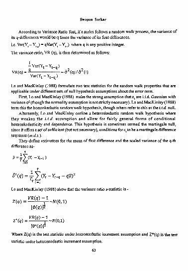
According to Variance Ratio Test, if a series follows a random walk process, the variance of its q-differences would be q times the variance of its first differences.

i.e. Var(Y, - v, .. ) = qVar(Y, - Y,.,) where q is any positive integer.

The variance ratio, VR (q), is then determined as follows:

Lo and MacKinlay (1988) formulate two test statistics for the random walk properties that are applicable under different sets of null hypothesis assumptions about the error term.

First, Lo and MacKinlay (1988) make the strong assumption that E, are i.i.d. Gaussian with variance a'(though the normality assumption is not strictly necessary). Lo and MacKinlay (1988) term this the homoskedastic random walk hypothesis, though others refer to this as the i.i.d null.

Alternately, Lo and MacKinlay outline a heteroskedastic random walk hypothesis where they weaken the i. i.d. assumption and allow for fairly general forms of conditional heteroskedasticity and dependence. This hypothesis is sometimes termed the martingale null, since it offers a set of sufficient (but not necessary), conditions for E, to be a martingale difference sequence (m.ds.).

They define estimators for the mean of first difference and the scaled variance of the q-th difference as-

- 1 r µ=ricr. -r,_,J t=l

BZ(q) = f i (Y, - l',-q - qµ)Z q t=l

Lo and Mac Kin lay (1988) show that the variance ratio z-statistic is -

VR(q)-1 Z(q) = 1 -N(O, 1)

[!Zi(q)Jz

Z"(q) = VR(q) -/ -N(0,1) [!Zi"(q)]!

Where Z( q) is the test statistic under homoscedastic increment assumption and Z*( q) is the test

statistic under heteroscedastic increment assumption.

63

Business Studies-Vol : XXXV & XXXVI, 2014 & 2015

Here f/l (q) and f/l* (q) are defined as -

"'( ) = 2(2q-l)(q-1) ., q 3qT

q-1 2

Q)'(q) = L [2(q - jl t U) j=I q

Where 8 U) is defined as -

t U) = { i: (y,_, - µ)'(y, - ~)·} /{ i: (y,_, - µ)2}2 t=J+l t•j+1

Now if the test statistics are found to be statistically significant it will indicate that the return

series do not follow random walk.

8. Data Analysis and Findings Descriptive Statistics For the purpose of analysis the study has employed E-views 7 and SPSS 11.5. The descriptive statistics of return series for indices have been reported in Table 1 below. The results relating to descriptive statistic show that all the four BSE Indices are negatively skewed with very low mean and variance suggesting lower expected returns and risk. The measure of kurtosis (more than 3 in all cases) suggests that the daily index return series in BSE have fatter tails than the normal distribution over the period. This is termed as Lepta-kurtosis, or simply 'fat tails'. Jarque-Bera (JB) statistic with significant p value indicates that the return series are not normal.

Table-1: Descriptive Statistics for the Indices under Study

Indices N Minimum Maximum

BSE30 2483 -0.11604 0.159900

BSEI00 2483 -0.11689 0.154902

BSE200 2483 -0.11345 0.151082

BSE500 2483 -0.11096 0.146179

Note: ** S1gmficant at I% level.

Results of Tests Applied

Serial Correlation Test Results

Mean Std. Skewness Kurtosis Deviation

0.000581 0.015645 -0.08819 11.13530

0.000577 0.015581 -0.10542 11.13168

0.000559 0.015334 -0.17289 11.14690

0.000555 0.015071 -0.26738 11.11535

Jarque-Bera

6850.421 ••

6845.705**

6979.111**

6843.243**

Serial Correlation test has been applied on all the four selected index return series under BSE up to 16 lags. The findings are shown under Table 2. The results reveal that the serial correlation

64

Swapan Sarkar

coefficients at lag I are significant at I% level for all four indices. The same are also significant at some higher lags (8 and 14). Existence of such significant correlation clearly indicates that the return series under study do not exhibit random behaviour.

Tuble-2: Results of Serial Correlation Test and Ljung-Box (Q) Statistic

SENSEX BSEI00

Lag AC Q-Stat Prob AC Q-Stat Prob AC

I 0.074 .. 13.714 o•• 0.09 .. 20.124 o•• 0.099**

2 -0.032 16.334 o•• -0.015 20.667 0" -0.006

3 -0.022 17.569 0.001** -0.009 20.878 0" -0.003

4 -0.03 19.882 0.001** -0.031 23.258 o•• -0.03

5 -0.018 20.682 0.001 .. -0.015 23.846 0" -0.014

6 -0.032 23.253 0.001** -0.029 25.936 0" -0.027

7 0.015 23.778 0.001 .. 0.022 27.132 0" 0.026

8 0.058 .. 32.151 o•• l.058' 35.471 0" K).057"

9 0.02 33.118 0" 0.028 37.419 0" 0.029

10 0.011 33.445 0" 0.013 37.82 0" 0.014

II -0.009 33.632 0" -0.013 38.222 0" -0.013

12 0.006 33.71 0.001 .. 0.004 38.266 0" 0.006

13 0.025 35.222 0.001•• 0.028 40.197 0" 0.03

14 0.046' 40.444 0" J.054' 47.498 0" 0.056"

15 0.006 40.536 0" 0.012 47.86 0" 0.014

16 0.005 40.603 0.001** 0.011 48.143 0" 0.014

Note: "' Significant at 5o/o level and ** Significant at 1% level

Ljung-Box (Q) Statistic Test Results

BSE200 BSE500

Q-Stat Prob AC Q-Stat

24.585 o•• 0.111** 30.736

24.673 0" 0.002 30.748

24.689 0" 0.008 30.912

26.901 o•• -0.026 32.531

27.375 0" -0.011 32.839

29.256 0" -0.025 34.374

30.889 0" 0.029 36.502

39.065 0" 0.057** 44.739

41.192 0" 0.031 47.145

41.707 0" 0.016 47.801

42.139 0" -0.011 48.111

42.239 0" 0.008 48.271

44.427 0" 0.031 50.7

52.295 0" 0.06** 59.608

52.785 0" 0.015 60.161

53.255 0" 0.016 60.801

Prob

o•• 0"

0"

o•• 0"

0"

0"

0"

0"

0"

0"

0"

0"

0"

0"

0"

The results of Q statistic have also been reported in Table 2. The findings suggest that the Q statistic is significant at I% level for all the lags for each of the indices under study. This is a clear indication that all the index return series have failed to exhibit any random movement.

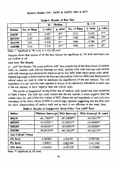
Run Test Results

The descriptive statistics of the selected index returns in the study shows that the return series have significant Jarque-Berra statistics thereby clearly indicating that they do not follow normal distribution. Hence use of a non parametric run test becomes more meaningful. Thus Run Test has been used as a complementary test to the serial correlation test. Both median values and Zero value have been used as the cut-off point. The results of Run Test have been incorporated under Table 3 as follows-

65

Business Studieo-Vol : XXXV & XXXVI, 2014 & 2015

Table-3· Results of Run Test

K= Median K- 0

Indices No. of Runs Z value p value No. of Runs Z value p value

BSE30 IIS7 -3.432 o•• 1147 -3.542 o•• BSE100 1147 -3.834 o•• 1103 -5.098 o•• BSE200 1241 -4.476 o•• 1094 -5.384 o•• BSES00 1115 -5.118 o•• 1092 -5.432 o••

Note: ** S1gmficant at I% level, K = Cut off pomt

Analysis shows that returns of all the four indices are significant at I% level and hence are

not random at all.

Unit Root '.lest Results (i) A.DF Test Results: The study performs ADF Test considering all the three forms of random walk, i.e., random walk without intercept (or drift), random walk with intercept and random walk with intercept and deterministic trend on all the four BSE index return series under study. Optimal lag length is determined by the Schwarz Information Criterion (SBC) and MacKinnon 's critical values are used in order to determine the significance of the test statistic. The null hypothesis of a unit root has been rejected in favour of the stationary alternative in each case if the test statistic is more negative than the critical value.

The results of Augmented Dickey-Fuller test of random walk model has been presented in Table 4 below. The ADF test result reveals that the test statistic is more negative than the critical value for each of the four indices of BSE. Hence the null hypothesis of unit root (non stationary) of the index returns of BSE is convincingly rejected, suggesting that the BSE does not show characteristics of random walk and as such is not efficient in the weak form.

Table-4: Results of Augmented Dicky-Fuller Test (ADF Test)

Indices Wiithout Intercept With Intercept With intercept & trend

BSE30 -46.17849** -46.22848** -46.22671 ••

BSEI00 -45.45553•• -45.50354** -45.49969**

BSE200 -45.02542** -45.07091 •• -45.06480**

BSES00 -44.49320** -44.53856** -44.53272**

Test Critical Values

1% level -2.565894 -3.432791 -3.961742

5% level -1.94051 -2.862504 -3.411618

10% level -1.616614 -2.567328 -3.127680

Note: •• S1gmficant at I% level.

66

Swapan Sarkar

(ii) Phillips-Perron (PP) Test Results

This study has perfonned PP test as a confinnatory data analysis. PP test has been perfonned on all the BSE index return series under study. Optimal bandwidth is detennined by the Newey­West Criterion using Bartlett kernel and MacKinnon's one sided p values are used in order to determine the significance of the test statistic. Finally, the null hypothesis of a unit root has been rejected in favour of the stationary alternative in each case if the test statistic is more negative than the critical value.

The results of Philips-Perron (1988) test of random walk model has been presented in Table 5. The PP test results reveal that the test statistic is more negative than the critical value for all the four indices of BSE. Hence, the results strongly reject the null hypothesis of unit root (non stationary) of index returns of BSE thereby suggesting that BSE index returns do not show any characteristics of random walk.

Table-5: Results of Philips-Perron Test (PP Test)

Indices Without Intercept

BSE30 -46.07181**

BSElO0 -45.33234**

BSE200 -44.96365**

BSES00 -44.52292**

Test Critical Values

1% level -2.565894

5% level -1.94051

10% level -1.616614

Note: ** Significant at I% level.

Variance Ratio Test Results

With Intercept With intercept & trend

-46.16583** -46.19295**

-45.36751 •• -45.36277**

-44.96703** -44.97413**

-44.54336** -44.53629**

-3.432791 -3.961742

-2.862504 -3.411618

-2.567328 -3.127680

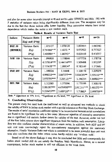
The study performs Variance Ratio Test for both the assumptions of homoscedastic and heteroscedastic increments. Moreover, the variance ratio is calculated for intervals ( q) of 2, 4, 8 and 16. For each interval, we report, the estimate of the variance ratio, VR (q), and the test statistics for the null hypotheses of homoscedastic {Z(q)) and heteroscedastic, {Z*(q)} increments' random walks. The results have been reported in Table 6 below.

Empirical evidences obtained from the variance ratio test indicate that the random walk hypothesis under the homoscedastic increment assumption is rejected at 1 %, 5% or 10% level for all the four BSE index return series ( except for m=8 and m= 16 under SENS EX and for m=8 under BSE 100) as the Z statistics of variance ratios are significantly different from one.

Similarly the empirical findings also reveal that the null hypothesis of random walks under the assumption of heteroscedastic increments is also rejected for all the index returns for m=2

67

Business Studie5-Vol : XXXV & XXXVI, 2014 & 2015

and also for some other intervals (except m=8 and m=l6 under SENSEX and BSE 100) with z statistics of variance ratios being significantly different from one. The exception may be due to the fact that those indices offer better liquidity. Thus successive returns have serial

dependence which makes the series a non random walk.

Tabl~· Results of Variance Ratio Test

Indices Variance Ratio m=2 m=4 m=8 m=l6

Z(q) and Z*(q)

BSE 30 Variance Ratio 1.075137 1.070130 1.001954 1.063383

(SENSEX) Z(q) 3.744060* .. 1.66721* 0.032922 0.717527

Z*(q) 2.405004** 1.86792* 0.020100 0.436927

BSE 100 Variance Ratio 1.090850 1.118044 1.077736 1.170716

Z(q) 4.527014*** 3.144114*** 1.309498 1.93259*

Z*(q) 2.755678*** 1.88874* 0.783149 1.173663

BSE 200 Variance Ratio 1.100326 1.14448 1.120174 1.229239

Z(q) 4.999232*** 3.847377*** 2.024393** 2.59511 o••• Z*(q) 2.970795*** 2.265121 •• 1.196234 1.569855***

BSE 500 Variance Ratio 1.112085 1.175594 1.175199 1.308578

Z(q) 5.581587*** 4.676958*** 2.951311*** 3.493273***

Z*(q) 3.223435*** 2.689728*** 1.71862* 2.098758**

Note: * Significant at 10% level, **Significant at 5% level, *** Significant at I% level

9. Concluding Observations

The present study has used both the traditional as well as advanced test methods to check the validity ofRWH in Indian stock market with a special reference to Bombay Stock Exchange. The results of serial correlation coefficient appear to be inconclusive because serial correlations are found to be significant for only a few cases. Moreover rejection of normality assumption due to significant J-B statistic further deters the validity of the test. However, under run test all the four index returns show significant departure from the random walk assumption. Ljung­Box test also confirins similar characteristics of return series. In addition, both ADF and PP unit root tests convincingly reject the non-stationary assumption against the stationary alternative. Finally Variance Ratio test which is considered to be more powerful than unit root tests also confirms that the index return series hardly exhibit any 'random walk'.

Based on all the above findings it may thus be concluded that BSE and consequently the Indian stock market still do not satisfy the Random Walk Hypothesis. Hence, as a natural consequence, Indian stock market is still not efficient in the weak forin.

68

Swapan Sarkar

References .... (1981). "Likelihood Ratio Statistics for Autoregressive Time Series with Unit Root", &onometrica, 49,

1057-1072 . . . . .. ( I 988b ). "Permanent and Temporary Components of Stock Prices", Juurna/ of Political Economy, 96,

246-273. Bachelier, L. (1900) trans. James Boness. "Theory of Speculation", in Cootner (1964), 17-78.

Barua, S.K. (198 I). ''Tho Short run Price Behaviour of Securities- Somo Evidence of Efficiency on Indian Capital market", Vikalpa, 6(2).

Barua, S.K. and Raghunathan, V. (1987). "Inefficiency and Speculation in the Indian Capital Market'', Vikalpa, 12(3), 53-58.

Barua, S.K., Raghunathan, V. and Venna, J.R. (I 994). "Research on Indian Capital market: A Review", Vikalpa, 19(1), 15-31.

Chakraborty, M. (2006). "On validity of Random Walk Hypothesis in· Colombo Stock Exchange, Sri Lanka", Decision, 33(1), 135-161.

Cowles, A. and Jones, H. ( I 937). "Some A Posteriori Probabilities in Stock Market Action", &onometri.ca, 5, 280-294.

Cutler, D.M., Porterba, J.M. and Summers, L.H. (1990). "Speculative dynamics and the role of feedback traders", Ainerican Economic Review, 80 (2), 63-68.

Daniel, S. and Samuel, L. (2006). ''The Efficiency of Selected African Stock Markets", Finance India, xx (2), 553-571.

David, W. (I 997). "Variance Ratio tests of random walks in Australian Stock Market Indices", Working Paper, Unionvorsity of Western Australia.

Dickey, D. A. and Fuller, W. A. (1979). "Distribution of the estimates for autoregressive time series with a unit root", Journal of American Statistical Association, 14, 427-431.

Fama, E. (1965). "The Behavior of Stock Market Prices", Juurnal of Business, 38, 34-105.

Fama, E. and French, K. (1988a). "Dividend Yields and Expected Stock Returns", Journal of Financial Economics, 22, 3-25.

Gupta, O.P. (1985). Behaviour of Share Prices in India: A Test of Market Efficiency, National, New Delhi.

Kendall, M. (1953). "The Analysis of Economic Time Series", Juurnal of the Royal Statistical Society, Series A, 96, 11-25.

Kim, M.J., Nelson, R.C. and Startz. (1991). "Mean reversion in stock prices? A reappraisal· of the empirical evidence", The Review of Economic Studies, SB, 515-528.

Kulkarni N. S. (1978). "Share Price Behaviour in India: A Spectral Analysis of Random Walk Hypothesis", Sankhya, The Indian Journal of Statistics, 40 (D), 135-162.

Lo, A. W. and MacKinlay, A.C. (1988). "Stock market prices do not follow random walks: Evidence from a simple specification test", The Review of Financial Studies, 1 (1), 4Hi6.

Mishra, P.K. (2010). "Indian Capital M•.rlcet- Revisiting Market Efficiency", http://www.ssm.com (last accessed on 25.06.2016). '

Obaidullah, M. (1991). "The Price/Earnings Ratio Anomaly in Indian Stock Markets", Decision, 18, 183.

69

Business Studies-Vol: XXXV & XXXVI, 2014 & 2015

Olowe. (1999). "Weak Fonn Efficiency of the Nigerian Stock Market: Further Evidence", African Development Review, 11 (I), 54-68.

Osborne, M.F.M. (1959). "Brownian Motion in the Stock Market'', Operations Research, 1, 145-173.

Pandey, A. (2003). "Efficiency of Indian Stock Market'', A Part of Project Report, Indira Gandhi Institute of Development and Research (IGIDR), Mumbai, India.

Phillips, P. and Perron, P. (1988). "Testing for a Unit Root in Time Series Regression", Biometrica, 75, 335-346.

Poshakwale, S. (I 996). "Evidence on Woak Fonn Efficiency and Day of tho Woek Effect in the Indian Stock Market", Finance India, X (3), September. 1996.

Poterba, J. and Summers, L. (1988). "Mean Reversion in Stock Prices: Evidence and Implications", Journal of Financial Economics, 22, 27-59.

Ramachandran, J. (1985). "Behaviour of Stock Market Prices, Trading Rules, Infonnation & Market Efficiency", Doctoral Dissertation, Indian Institute of Management, Ahmadabad.

Rao, K.N. (1988). "Stock Market Efficiency: The Indian Experience", Proceedings of National Seminar on Indian Securities Market: Thrust and Challenges, March 24-26, 1988, University of Delhi.

Rao, N.K. and Mukherjee, K. (1971). "Random Walk Hypothesis: An Empirical Study", hthaniti, 14 (I & 2), 49-53.

Ray, D. (1976). "Analysis of Security Prices in India", Sanlchya, 38 (C), 149-164.

Roberts, H. (1959). "Stock Market 'Pattoms' and Financial Analysis: Methodological Suggestions", Journal of Finance, 44, 1-10.

Samuelson, P. (1965} "Proof That Properly Anticipated Prices Fluctuate Randomly", Industrial Management Review, 6, 41-49.

Sharma, J.L. (1983). "Efficient Capital Markets and Random Character of Stock Price Behaviour in a Developing Economy", Indian Economic Journal, 31(2), 53-70.

Sharma, J.L. and Kennedy, R.E. (1977). "A Comparative Analysis of Stock Price Behaviour on the Bombay, London and New York Stock Exchanges", Journal of Financial and Quantitative Analysis, Sep. 1977.

Shiguang. Ma and Michelle, L.B. (2001). "Are China's Stock Markets Really Weak fonn Efficient?", A.de/aide Australia Discussion Paper, Centre for International Economic Studies, 119, 1-47.

Srinivasan, P. (20 IO). "Testing Weak Fonn Efficiency oflndian Stock Markets", AP JRBM, I (2), November 2010.

Working. H. (1934). "A Random Difference Series for Use in the Analysis of Time Series". Journal of the American Statistical Association, 29, 11-24.

Yalawar, Y.B. (1988). "Bombay Stock Exchange: Rates of Return and Efficiency", Indian Economic Journal, 36(4), 68-121.

70