revision of NBER Working Paper No. 9018 (June 2002)

Child Labor: The Role of Income Variability and Credit Constraints

Across Countries*

Rajeev H. Dehejia Department of Economics and SIPA

Columbia University and NBER

Roberta Gatti Development Research Group

The World Bank

This version: June 2003

Keywords: child labor; financial markets development; poverty.

JEL codes: J22, G1, O16.

*We thank Jagdish Bhagwati, David Dollar, and Alan Krueger for helpful conversations, Kathleen Beegle, Maria Solededad Martinez Peria, Antonio Spilimbergo and seminar participants at the World Bank, the Inter-American Development Bank, and at the LACEA 2002 meetings for useful comments, and Sergio Kurlat for excellent research assistance. All errors are our own. Dehejia thanks the National Bureau of Economic Research and the Industrial Relations Section, Princeton University, for their kind hospitality. The opinions expressed here do not necessarily represent those of the World Bank or its member countries. Address correspondence to rd247@columbia.edu.

Child Labor: The Role of Income Variability and Credit Constraints Across Countries Rajeev Dehejia and Roberta Gatti JEL No. J22, G1, O16

ABSTRACT

This paper examines the relationship between child labor and access to credit at a cross-

country level. Even though this link is theoretically central to child labor, so far there has

been little work done to assess its importance empirically. We measure child labor as a

country aggregate, and credit constraints are proxied by the extent of financial

development. These two variables display a significant negative relationship, which is

particularly strong in the sample of low income countries. We show this relationship to

be robust to selection on observables (by controlling for a wide range of variables such as

GDP per capita, urbanization, initial child labor, schooling, fertility, legal institutions,

inequality, and openness), and to selection on unobservables (by allowing for fixed

effects). Moreover, we find that, in the absence of developed financial markets,

households appear to resort substantially to child labor in order to cope with income

variability. This suggests that smoothing of income shocks is one of the channels through

which financial development affects child labor and that, as a result, policies aimed at

widening households’ access to credit could be effective in reducing the extent of child

labor.

Rajeev Dehejia Roberta Gatti Department of Economics and SIPA Development Research Group Columbia University The World Bank , MC3-353 420 W. 118th Street, Room 1022 1818 H Street, N.W. New York, NY 10027 Washington, DC 20433 and NBER rgatti@worldbank.org rd247@columbia.edu

1

1. Introduction

Child labor has been a concern of policy since at least the 19th Century (see Basu (1999),

Section 2.2), and the debate on which policies should be employed to reduce it − ranging

from legislative bans on child labor, to trade sanctions against countries that use child

labor, to schooling subsidies for children − is long-standing. As troubling as child labor is

per se, it is essential to investigate its economic determinants in order to inform policy

choices and identify their welfare implications.

The evidence and existing literature suggest a strong link between child labor and

poverty (Krueger (1996)). In 1995 there were an estimated 120 million children engaged

in full-time paid work (see ILO (1996)). In the same year, the incidence of child labor

was 2.3% among countries in the upper quartile of GDP per capita, and 34% among

countries in the lowest quartile of GDP per capita. If this link is causal and there are no

market inefficiencies, we would expect promoting general economic development to

reduce child labor. However, other mechanisms can also account for the observed

relationship between child labor and poverty. In particular, market failures – which are

arguably more common where poverty is widespread – or externalities might be the

actual cause of child labor. For example, if private returns to education are lower than

social returns, child labor can be inefficiently high. In this case, government intervention

in the specific market where the inefficiency occurs is to be preferred (Grootaert and

Kanbur, (1995)).

The work in this paper goes in this direction. In particular, we explore the nexus

between child labor and one possible source of inefficiency − credit constraints. The

basic intuition is that child labor creates a trade-off between current and future income.

Putting children to work raises current family income, but by interfering with children’s

human capital development, it reduces future income. In this context, credit constraints

can play an important role, by preventing households from optimally trading off current

income against future returns. By entering the job market, a child immediately

contributes to household income, but, to the extent that current work displaces schooling,

this carries a future cost in terms of reduced earnings potential. Access to credit also

2

allows households to also smooth transitory earnings shocks without recourse to child

labor.

Even though access to credit is central to child labor theoretically, there has been

little work done to assess its importance empirically (see Brown, Deardorff, and Stern

(2001)). In this paper, we pursue a cross-country strategy. We measure child labor as a

country aggregate, and credit constraints are proxied by the extent of financial

intermediation at the country level. These two variables display a strong negative

(unconditional) relationship (see Figure 1). Of course, to determine the strength of the

relationship we must control for other potentially important covariates. The existing

literature on child labor provides some guidance. Most empirical studies on child labor

suggest income is a crucial variable. Likewise, the literature suggests that schooling,

fertility patterns, ruralization, and openness might also be important determinants of child

labor.

Our results show a strong link between child labor and access to credit even after

controlling for a range of other variable and using a range of estimation techniques. We

also find that income variability has a sizeable, positive impact on child labor in countries

where financial markets are underdeveloped, but this is not the case when financial

markets are developed. This suggests that households resort to their children’s work to

cope with income shocks and that access to credit might effectively cut households’

demands on children’s time. We then focus on the subset of low-income countries –

countries which have both less developed financial markets and a greater prevalence of

child labor and, as such, are of greater policy interest. We find that the relationship

between financial development and child labor is robustly and significantly negative, and

sizeable. Moreover, this association persists after allowing for country fixed effects,

suggesting that improvements in financial development are strongly associated with

decreases in child labor within countries.

The cross-country strategy we pursue in this paper has a number of strengths.

First, there is a substantial amount of variation in the prevalence of child labor across

countries and over time. Moreover, much of this variation can be explained by factors

(such as laws, institutions and openness) that inherently vary at the country level. Among

these, is the extent of access to credit, which is itself influenced by a country’s financial

3

institutions. Of course there is also significant within-country variation that is best

understood using microeconometric evidence. However, in the absence of policy

experiments, it is notoriously difficult to find satisfactory direct measures of access to

credit directly at the disaggregated, household level. Furthermore, microeconometric

findings are typically country-specific, while the evidence we present here has the

advantage of representing trends that can be generalized to many countries and

encompass a relatively long time span (1950 to 1995).

Though our approach has its strengths, we view our paper as being

complementary to micro-data empirical work examining the relationship between credit

constraints and child labor. Indeed, three such papers have been written subsequent to the

present work (Beegle, Dehejia, and Gatti (2002), Edmonds (2002), and Guarcello et al.,

(2002)).

Our results are important for a number of reasons. First, we establish the

empirical relevance of a significant strand of the theoretical literature on child labor by

highlighting the significant negative relationship between the development of financial

markets and child labor. Second, we show that this relationship holds even after

controlling for a wide range of covariates which include income levels (usually identified

as the major determinant of child labor) and for country fixed effects. Finally, our results

clearly point to a policy mechanism – widening access to credit – that might help to

alleviate the problem of child labor and that, to some extent, is independent of raising per

capita income and solving the more complex problem of general economic development.

The paper is organized as follows. Section 2 reviews the relevant literature.

Section 3 describes the data and presents our results. Section 4 examines the robustness

of our results. Section 5 concludes.

2. Review of the Literature

The empirical literature on child labor is vast (see Brown, Deardorff, and Stern (2001)),

and the more recent theoretical literature is also substantial (see Basu (1999)). In this

section, we highlight the papers that are essential to our empirical strategy.

4

2.1 The Modeling Framework

Basu (1999) partitions the theoretical literature on child labor into two groups −

papers that examine intra-household bargaining (between parents, or parents and

children) and those that examine extra-household bargaining (where the household is a

single unit and bargains with employers).

In the intra-household bargaining framework, child labor is the outcome of a

bargaining process between members of the household, for example parents and children

(see Bourguignon and Chiappori (1994) and Moehling (1995)) or the father and the

mother (who is assumed to care for the children more than the father, see Galasso

(1999)). The weight that each member receives can depend upon his or her contribution

to the family’s resources. Collectively, child labor may be desirable because it contributes

to the family income, and it may be desirable to the child because it increases his or her

weight in the family decision function. Within this framework the key variables are those

that determine the relative bargaining strength of different members of the household.

This could include wealth, the number, age, and gender of children, and earnings (wages)

if an individual were to work (regardless of whether this is observed or not).

The extra-household bargaining framework considers each household as a unitary

entity (see, amongst others, Becker (1964) and Gupta (1998)). The motivation behind this

approach is that children’s bargaining power is inherently very limited, so that parents

determine to what extent a child works without necessarily considering the child’s

welfare.1 The parents and the employer bargain about the child’s wage and the fraction of

that wage to be paid as food to the child. Within this framework the key variables are

those that determine the relative bargaining strength of the household vis à vis the

employer. These also include household wealth variables as well as access to credit.

1 However, if parents are altruistic, they face a meaningful trade-off between the benefit of child labor and its cost. We will discuss this mechanism in detail in Section 2.2.

5

2.2 The Role of Access to Credit

The role of credit markets in determining the extent of child labor has been

addressed by a recent strand of the theoretical literature (Parsons and Goldin (1989),

Baland and Robinson (2000), Ranjan (1999, 2001) and Rosati and Tzannatos (2000)).

Analytically, this question is closely related to the literature on bequests within altruistic,

unitary models of the family à la Becker (1974). That literature has highlighted that the

non-negativity constraint in bequests can lead to an inefficient allocation of resources

within the family (see for example Becker and Murphy (1988)). In particular, if parents

care about their children but bequests are at a corner, child labor is not generally efficient.

The basic intuition is that child labor creates a trade-off between current and future

income. Putting children to work raises current family income, but by interfering with

children’s human capital development, it reduces future income. This future income is, of

course, realized by the children and not the parents. Thus, if there are positive bequests,

parents can compensate themselves for foregone current income by reducing bequests.

Conversely, if bequests are at a corner – which is more likely to occur for poorer

households – parents will tend to draw on child labor too heavily.

Even if conditions exist for an efficient allocation of child labor from an

intergenerational perspective (i.e., bequests are positive), parents might still choose an

inefficiently high level of labor for their children if they cannot borrow to smooth their

consumption over time, i.e. if the intragenerational allocation of resources is constrained.

The following model, adapted from Baland and Robinson (2000), illustrates this point

analytically.

Consider a two-period model where the parent and the child live

contemporaneously. In each period the parent supplies labor inelastically, earning income

A. In period 1, the parent decides how much to save for the following period, s, as well as

the extent to which his child will work, ]1,0[∈cl . When working in period 1, the child

earns lc, which the parent can appropriate completely. In period 2, the child, now an

adult, will supply one unit of labor, which will earn her an income of )1( clh − , where h is

the human capital accumulated in period 1. h(·) is decreasing in lc and is strictly concave,

with h(0)=1.

6

We assume that the parent is altruistic. He cares about his own consumption in

periods 1 and 2, 1pc and 2

pc respectively, and, to the extent λ, about the child’s utility.

Because of altruism, in period 2 the parent might want to leave a bequest b to the child.

For simplicity, parental utility is additively separable and there is no intertemporal

discount. The child is selfish and cares only about her own consumption cc (for further

simplicity, the child only consumes in period 2).

The parent’s utility function is

)()()( 21ccppp cWcucuW λ++=

where )( cc cW is the child’s utility function and u(·) and Wi(·) are concave and well-

behaved functions.

The parent’s budget constraints in periods 1 and 2 are:

slAc cp −+=1

and

sbAc p +−=2 .

The child’s budget constraint is

blhc cc +−= )1( .

In order to illustrate how inefficiently high child labor might emerge if individuals

cannot borrow, we focus on the case where bequests are positive but 0≥s .2 The first

order conditions are as follows:

(1) with respect to b )()(' '2ccp cWcu λ= if b>0

(2) with respect to s )(')(' 21pp cucu ≥ if s>0

(3) with respect to lc )1(')()(' '1cccp lhcWcu −= λ

In this setup, the chosen level of child labor is efficient when the marginal return

to time spent in school equals its marginal cost (the opportunity cost of child labor). Here

the return to education is )1( clh − and the opportunity cost of child labor is lc. Efficient

2 For simplicity, we allow only transfers from the parent to the child.

7

child labor is therefore defined by 1)1(' =− clh . Conversely, child labor is inefficiently

high if 1)1(' >− clh . Baland and Robinson (2000) show that if s=0 (i.e. if the borrowing

constraint is actually binding), the parent will choose to make his child work too much. If

in period 1 the parent wished he could borrow but cannot do so, his consumption will be

lower and its marginal utility higher than optimal, )(')(' 21pp cucu > . Substituting for

)(' 2pcu from (1) and )(' 1

pcu from (3), it easily follows that 1)1(' >− clh . Intuitively, if the

parent cannot smooth consumption between period 1 and 2 through borrowing, he will

use child labor to increase consumption in period 1 at the expense of his child’s human

capital accumulation.

This model suggests that the availability of credit should be a factor that predicts

the incidence of child labor. Moreover, finding evidence of such an effect will imply that

the child labor we observe is in fact inefficiently high. In the context of our cross-country

work, we will use the degree of development of financial markets in a country as a

measure of the credit constraints that individuals face.

2.3 Empirical Work

At the cross-country level, much work has gone into creating a uniform definition

of child labor. Two significant efforts in this direction are Ashagrie (1993) and Grootaert

and Kanbur (1995). These previous analyses are more concerned with measuring the

extent of child labor than with estimating the effect of various country characteristics on

the degree of child labor. More recently, there have been a number of studies examining

the relationship between child labor and specific factors contributing to child labor.

Krueger (1996) establishes a strong negative relationship between the prevalence of child

labor and national income, a finding which is confirmed in the present study. Krueger

also shows that there is little evidence (at least in the United States) that the support for

banning imports made with child labor is linked to the potential benefits to domestic rent

seekers (i.e., unskilled labor, who might benefit from such a ban). Cigno, Rosati, and

Guarcello (2002) examine the relationship between globalization (trade) and child labor.

Rogers and Swinnerton (2001) examine the relationship between income distribution and

8

child labor, arguing that increasing the equality of income distribution does not

necessarily lead to reductions in child labor.

At the level of micro data, there is a range of empirical studies that examine the

causes of child labor. In a recent volume, Grootaert and Patrinos (1999) review findings

from Côte D’Ivoire, Colombia, Bolivia, and the Philippines. Other authors have

examined child labor in Ghana (Canagarajah and Coulombe (1997)) and Vietnam

(Edmonds and Pavcnik (2001)). A consistent finding is that child labor is associated with

poverty. This, of course, is what we would anticipate, and it underlines the necessity of

controlling for income in our empirical analysis. Among other determinants of child labor

at the individual level are the child’s age and gender, education and employment of the

parents, and rural versus urban location. From this list, it is of course difficult at the

aggregate level to control for household-specific attributes such as gender composition

and age, but we can control for education and the degree of urbanization of a country.

Three recent papers, Beegle, Dehejia, and Gatti (2002), Edmunds (2002), and

Guarcello et al. (2002), examine the link between credit constraints and child labor using

micro data. All of these works find evidence for the role of credit constraints. As

suggested in the introduction, we view the current paper as being complementary to these

other papers as we are able to examine between-country variation and to address issues

(such as the development of financial markets) that are not easily captured at the

disaggregated level but that we can show to be relevant for child labor.

A related set of papers have examined the link between child labor and credit

constraints indirectly. The literature on the causes of child labor has noted a link between

household assets and child labor (see Grootaert and Patrinos (1999) and Brown,

Deardorff, and Stern (2001)). To the extent that assets can serve as collateral for

borrowing, this link suggests that access to credit might play a role. Of course, the

evidence is indirect, and might also be picking up wealth effects. There are also papers

that examine the link between credit and schooling choices. Jacoby and Skoufias (1997)

examine the completeness of credit markets in a dataset of six Indian villages. They find

that households are not fully able to insure themselves against unanticipated idiosyncratic

income shocks and, as a result, reduce schooling. Jacoby (1994), using data from Peru,

finds that children in households with lower levels of income and durable goods

9

(consequently, presumably with a lower access to credit) are more likely to repeat grades

at school. Flug, Spilimbergo, and Wachtenheim (1998) examine the effect of financial

development on schooling using cross-sectional country data, and find a negative and

significant effect. These papers are complementary to the present study, because – as

shown by Ravallion and Wodon (2000) for data from Bangladesh – schooling and child

labor are not necessarily one-for-one substitutes.

3. Data, Specification, and Results

The availability of child labor data (see below) allows us to build a panel for 172

countries for the years 1950-60, 70, 80, 90, 95. For this dataset we first estimate a

parsimonious specification where we control for some basic determinants of child labor.

We then add to this specification our variable of interest (a proxy for the availability of

credit within a country), and investigate whether access to credit is effective in

dampening risk by adding to the specification a measure of income volatility. In the next

section, we perform a number of robustness checks, which include estimating our

specification without outliers, adding to the regression a number of other variables that, if

not accounted for, might generate an omitted variable problem, and allowing for fixed

effects.

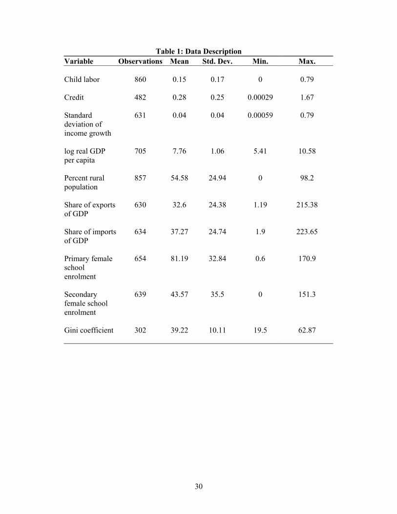
3.1 Data Description

We measure the extent of child labor (CHILDLAB) as the percentage of the

population in the 10-14-age range that is actively engaged in work. These data were

compiled by the ILO and are available at ten-year intervals starting from 1950 for 172

countries. “Active population” includes people who worked (for wage or salary, in cash

or in kind as well as for family unpaid work) for at least one hour during the reference

period (ILO (1996)). The structure of the data does not allow us to infer the intensity of

child labor, so that we cannot distinguish between light child work (that some might

argue to be beneficial for adolescents) and full-time labor that might seriously conflict

with human capital accumulation. Moreover, like most official data on child labor, these

10

data are likely to suffer from underreporting, as work by children is illegal or restricted

by law in most countries and children are often employed in the informal sector. These

problems notwithstanding, the ILO data has the advantage of being adjusted on a basis of

the internationally accepted definitions, thereby allowing cross-countries comparisons

over time (Ashagrie (1993)).

As a proxy for the absence of credit constraints we use the ratio of private credit

issued by deposit-money banks to GDP (the variable CREDIT, which we refer to

interchangeably as “access to credit” or “financial development”). This variable isolates

credit issued to the private sector (as opposed to credit issued to governments and public

enterprises) and captures the degree of activity of financial intermediaries that is most

relevant to our investigation: the channeling of savings into lending (Beck, Demirguc-

Kunt, and Levine (1999)). Indirect evidence suggests that financial development might be

a good proxy for the extent of credit constraints faced by households in an economy. For

example, using data on nearly 3,000 small- and medium-sized firms and 48 countries

from the World Business Environment Survey dataset, Beck et al. (2002) show that

financial development is negatively and significantly correlated with the degree of firms’

financing constraints (a correlation of -0.20, significant at 1%).3 As it is likely that small

and medium enterprises face financing problems similar to those of households, this

evidence lends support to our use of this proxy. Not surprisingly, financial development

is also negatively correlated with the spread between lending and deposit rates, which is

often interpreted as a measure of the cost of intermediation to households and firms (in

our sample, the correlation is –0.24, significant at 5%).

We should point out that financial intermediation has an effect not only on

households, but also on the producer side of the economy. As such our access to credit

proxy embodies both of these effects, and can be interpreted more broadly as capturing

the effect of financial development (see King and Levine (1993) and Rajan and Zingales

(1998)). To the extent that improved access to credit might lead to an increased demand

for child labor from firms, any negative relationship we uncover should be viewed as a

3 More precisely, it is correlated with enterprise managers’ perceptions about how large an obstacle financing issues are for their business. For more details, see Beck et al. (2002).

11

lower-bound estimate of the effect of financial development on the household supply of

child labor.

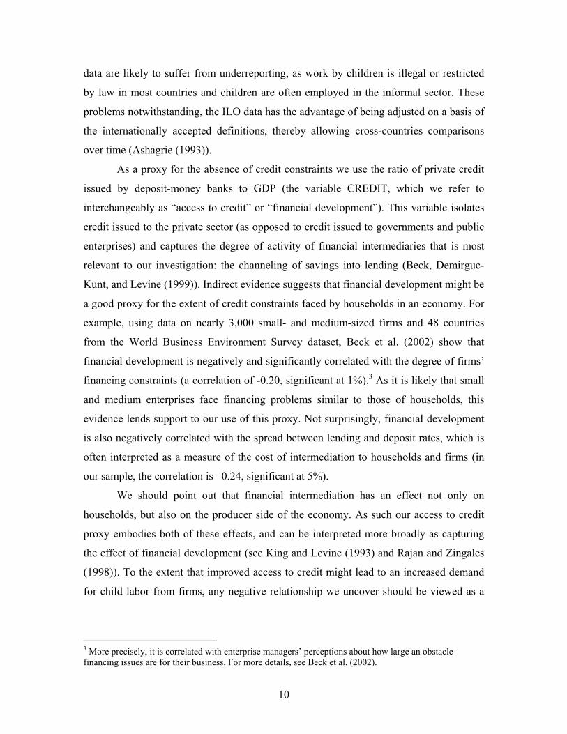
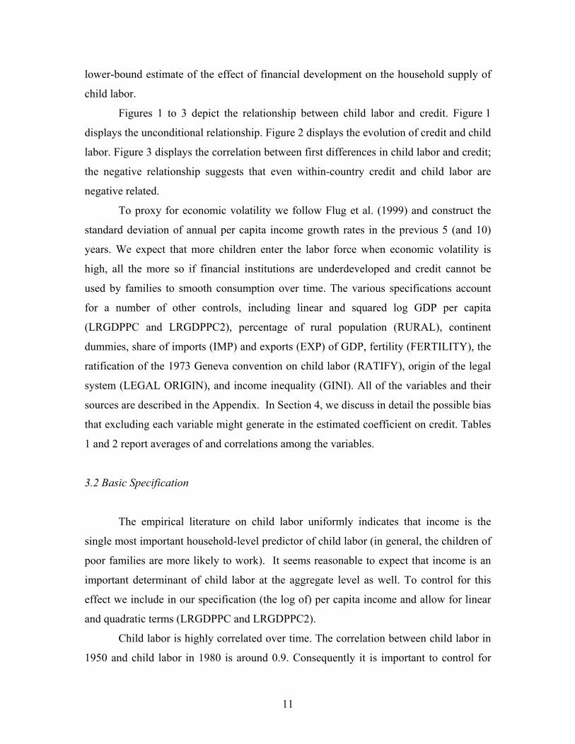
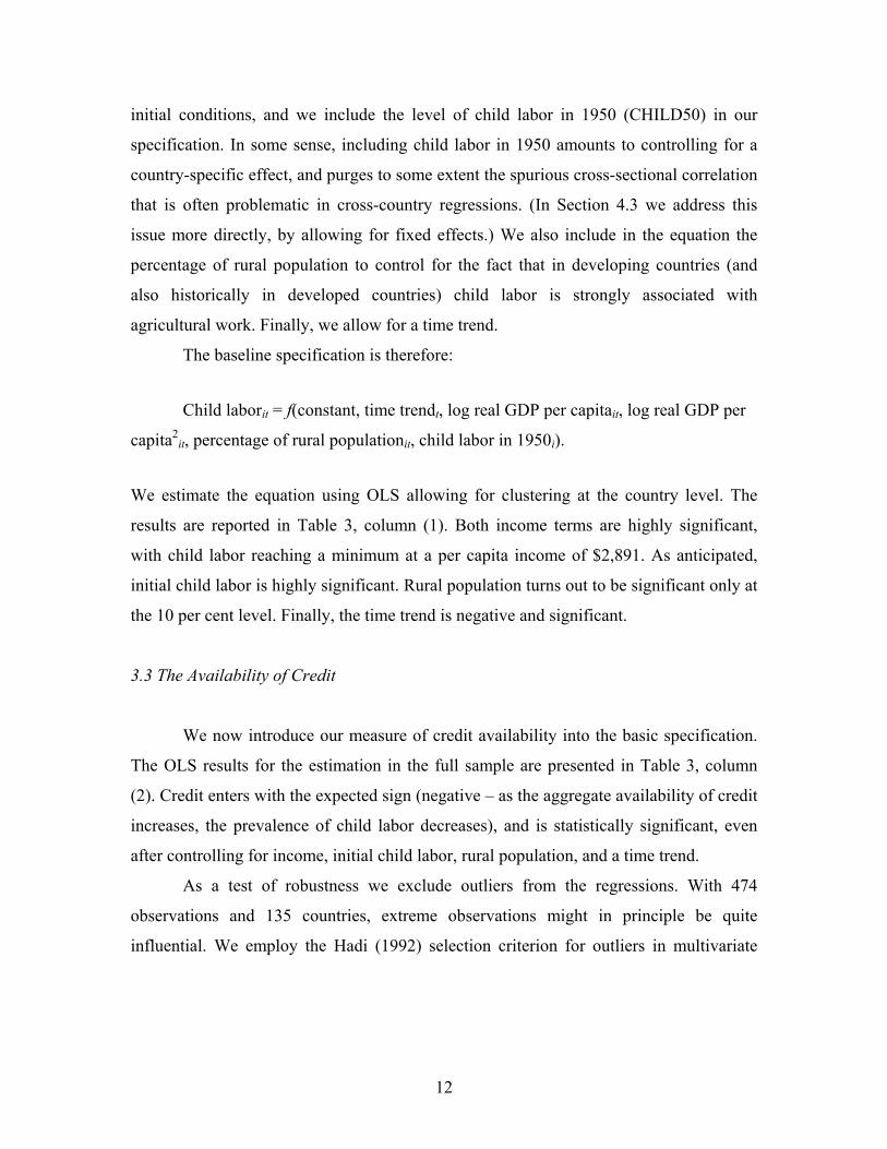
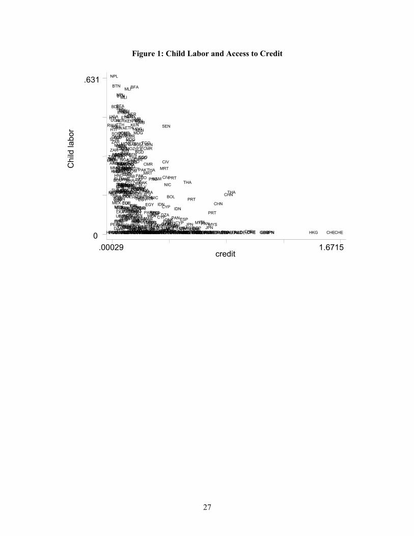
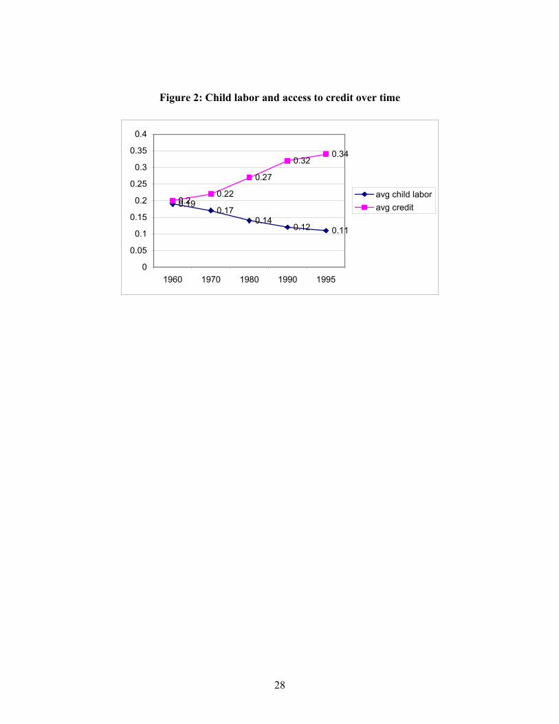
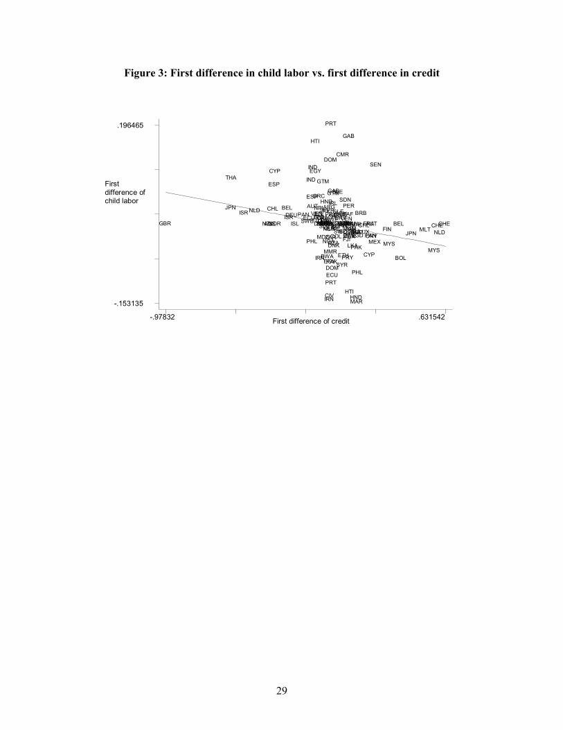
Figures 1 to 3 depict the relationship between child labor and credit. Figure 1

displays the unconditional relationship. Figure 2 displays the evolution of credit and child

labor. Figure 3 displays the correlation between first differences in child labor and credit;

the negative relationship suggests that even within-country credit and child labor are

negative related.

To proxy for economic volatility we follow Flug et al. (1999) and construct the

standard deviation of annual per capita income growth rates in the previous 5 (and 10)

years. We expect that more children enter the labor force when economic volatility is

high, all the more so if financial institutions are underdeveloped and credit cannot be

used by families to smooth consumption over time. The various specifications account

for a number of other controls, including linear and squared log GDP per capita

(LRGDPPC and LRGDPPC2), percentage of rural population (RURAL), continent

dummies, share of imports (IMP) and exports (EXP) of GDP, fertility (FERTILITY), the

ratification of the 1973 Geneva convention on child labor (RATIFY), origin of the legal

system (LEGAL ORIGIN), and income inequality (GINI). All of the variables and their

sources are described in the Appendix. In Section 4, we discuss in detail the possible bias

that excluding each variable might generate in the estimated coefficient on credit. Tables

1 and 2 report averages of and correlations among the variables.

3.2 Basic Specification

The empirical literature on child labor uniformly indicates that income is the

single most important household-level predictor of child labor (in general, the children of

poor families are more likely to work). It seems reasonable to expect that income is an

important determinant of child labor at the aggregate level as well. To control for this

effect we include in our specification (the log of) per capita income and allow for linear

and quadratic terms (LRGDPPC and LRGDPPC2).

Child labor is highly correlated over time. The correlation between child labor in

1950 and child labor in 1980 is around 0.9. Consequently it is important to control for

12

initial conditions, and we include the level of child labor in 1950 (CHILD50) in our

specification. In some sense, including child labor in 1950 amounts to controlling for a

country-specific effect, and purges to some extent the spurious cross-sectional correlation

that is often problematic in cross-country regressions. (In Section 4.3 we address this

issue more directly, by allowing for fixed effects.) We also include in the equation the

percentage of rural population to control for the fact that in developing countries (and

also historically in developed countries) child labor is strongly associated with

agricultural work. Finally, we allow for a time trend.

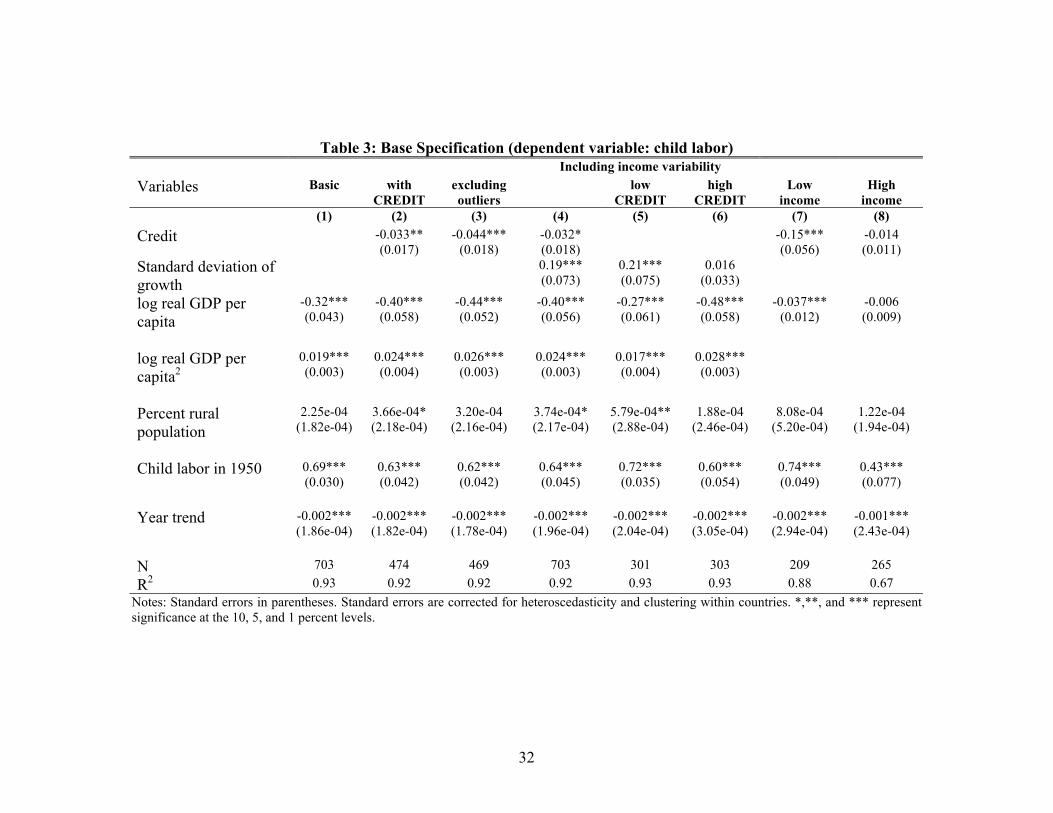
The baseline specification is therefore:

Child laborit = f(constant, time trendt, log real GDP per capitait, log real GDP per

capita2it, percentage of rural populationit, child labor in 1950i).

We estimate the equation using OLS allowing for clustering at the country level. The

results are reported in Table 3, column (1). Both income terms are highly significant,

with child labor reaching a minimum at a per capita income of $2,891. As anticipated,

initial child labor is highly significant. Rural population turns out to be significant only at

the 10 per cent level. Finally, the time trend is negative and significant.

3.3 The Availability of Credit

We now introduce our measure of credit availability into the basic specification.

The OLS results for the estimation in the full sample are presented in Table 3, column

(2). Credit enters with the expected sign (negative – as the aggregate availability of credit

increases, the prevalence of child labor decreases), and is statistically significant, even

after controlling for income, initial child labor, rural population, and a time trend.

As a test of robustness we exclude outliers from the regressions. With 474

observations and 135 countries, extreme observations might in principle be quite

influential. We employ the Hadi (1992) selection criterion for outliers in multivariate

13

regressions.4 Four countries (Myanmar, Hong Kong, Switzerland, and Zaire) are

identified as outliers in this context. We rerun the OLS specification without these

outliers. For OLS the magnitude of the coefficient of credit increases by 30%, and the

significance of the estimate is even stronger.

Our results confirm that the availability of credit – as proxied by financial

development – plays a significant role in explaining child labor. However, there are

several pathways through which this effect could operate, none of which is explicitly

captured by the specifications considered so far. For example, access to credit obviously

has an effect economic growth and long-run income, but by controlling for the level of

GDP per capita, we are accounting for this effect to some extent. In Table 3, columns (4)

to (6), we explore one possible mechanism − smoothing income shocks.

As outlined in Section 2, families might resort to sending their children to work to

help cope with negative income shocks. If credit is widely available, households can

instead borrow to smooth income variability and might not need to disrupt their

children’s education (or leisure time). When we introduce our measure of income

volatility (SDGROW5, the standard deviation of annual GDP growth in the previous 5

years) into the specification, we see that the estimated coefficient is large and highly

significant, suggesting that households indeed use child labor to cope with income

volatility.5 In principle, though, the variability of income should affect child labor mostly

in those countries where credit is not accessible. To investigate this possible effect, we

split the sample into high and low credit groups, using the mean or credit as the cutoff. In

Table 3, column (5), we see that for the low credit group, income variability enters the

specification significantly and the magnitude of the coefficient is substantial. Instead, for

the high credit group (columns (6)), the effect of income volatility on child labor is small

and not significantly different from zero.

The magnitude of the estimated coefficient on credit in the full sample is small,

relative for example to the effect of GDP per capita. For the OLS estimates, a one

standard deviation increase in access to credit is associated with a decrease of five per

4 Hadi’s (1992) technique is particularly useful to identify outliers in a multivariate regression setting and is based on a procedure that recursively defines distance of an observation from a cluster of observations in the model.

14

cent of a standard deviation in child labor. In contrast, the magnitude of the effect of GDP

per capita is much larger. If a country were to move from the 5th to the 10th percentile of

GDP per capita in 1995 (i.e., from $504 to $618), child labor would decrease by 3

percentage points, on a base prevalence of child labor of 39% for that level of income. In

contrast, moving between the same percentiles of access to credit would lead only to a

0.1 percentage point decrease in child labor. However, as we will see below, the

magnitude of the effect is much larger for the subsample of low-income countries. As

well, it is plausibly easier to increase household access to credit than to induce general

economic development, so it might be reasonable to consider larger increases in the level

of access to credit.6 For example, a move from the 25th to the 75th percentile of access to

credit would bring about a one percentage point, or 7 percent, decrease in child labor.

In columns (7) and (8), we examine our results for the sub-samples of rich and

poor countries (where we split the data by mean GDP per capita). This is a natural

dimension along which to search for heterogeneity in the effect of credit. We would

imagine the effect to be greater for poorer countries, where improvements in access to

credit are presumably extending the basic infrastructure of financial markets. Instead the

effect of access to credit in richer countries is presumably higher-order and less likely to

affect households. This is confirmed by our results in Table 3, columns (7) and (8). The

effect of credit is significant in both sub-samples, but is more than four times as large for

the sample of poor countries (and one third the magnitude for the rich sample).7

Thus, for the countries of greatest policy interest – poorer countries, which have

both a lower level of financial development and higher child labor – the magnitude of the

effect of credit is five times larger than for the overall sample. A move from the 25th to

the 75th percentile of credit is associated with a 5 percentage point decrease in child labor,

or a 17 percent reduction in child labor among low-income countries. In our subsequent

5 Results are virtually the same when instead of SDGROW5 we use SDGROW10, the standard deviation of annual GDP growth in the previous 10 years. 6 More precisely, though it is also difficult to increase the level of financial development of a country, it is presumably easier to increase household access to credit, which is the underlying variable of interest, for example by targeting credit to poorer households with children. 7 Splitting the sample by income levels inherently accounts for non-linearities in the relationship between income and child labor. Therefore we control for income linearly in the specifications run on the two sub-samples.

15

tables and discussion, we focus our attention on the low-income countries, since these are

the countries of greatest interest with respect to child labor.

4. Robustness Checks

A significant concern regarding our results in Section 3 is whether the effect of credit

availability on child labor reflects an actual link between the two variables or is instead

driven by spurious or omitted factors. Because of the interrelatedness of macro-level

variables, this is a typical concern with cross country regressions. To be able to rule out

these potential problems, we extend the empirical framework in several directions to

check for the robustness of our results. First, we consider the robustness of our results to

implementing Tobit estimation. Second, we consider additional control variables (hence

examine sensitivity to selection on observables). Third, we consider fixed-effects models

(hence examine sensitivity to selection on unobservables).

4.1 The Mass Point at Zero Child Labor

One important feature of data on child labor is the presence of a substantial

proportion of zeros. Of the 703 data points used in Table 3, column (1), over 20 percent

are zero. The OLS assumption of linearity (and implicitly normality for the standard

errors) might not be appropriate for this sample. Thus, we reestimate the specifications in

Table 3 using a Tobit, which explicitly allows for a mass point in the distribution of the

dependent variable.

In Table 4, column (1), we see that the sign and magnitude of the coefficients in

basic specification is very similar to Table 3, column (1). Likewise, in column (2), the

sign of the credit coefficients is the same as in Table 3, column (2), but the magnitude of

the impact is doubled. In column (3), we see again that the coefficient is not at all

sensitive to discarding outliers from the sample. In columns (4) to (6) we reexamine the

impact of aggregate income volatility on child labor. For the full and low-credit samples

the magnitude of the impact is essentially unchanged from Table 3, but for the high-credit

countries, income volatility now contributes significantly (though at the 10 percent level)

16

to child labor. However, the coefficient for the standard deviation of income growth is

much larger for low-income countries.

Finally, in columns (7) and (8) we consider the split-sample results. For the low-

income countries, the Tobit results are virtually identical to OLS. This is not surprising,

since so few of the observations are at the mass point. In contrast, for the high-income

sample, the credit effect is much larger in magnitude.

4.2 Additional Controls

We now subject our result to a battery of additional controls. In particular, we

focus on our results for the low-income sample, since this is the sample of greatest

interest. Our interest is not to interpret the additional coefficients causally, since some of

the variables we add are potentially endogenous with respect to child labor. The

additional controls are intended instead to confirm that the significance of credit is not

simply attributable to omitted variable bias. These estimates are reported in Table 5.

First, in order to control for systematic differences in the child labor intercept, we

add continent dummies (Table 5, column (1)). The magnitude of the credit variable

decreases only slightly, and remains significant at the 1 percent level. We retain continent

dummies in all of our specifications in Table 5.

We then control for primary and secondary (female) school enrollment (Table 5,

column (2)). The availability of education gives rise to an important inter-temporal trade-

off in the time allocation of children. Time spent in schoolwork may displace time spent

in work, but also creates a stream of future returns to education. Of course, schooling is

not a full-time activity, so this tradeoff may not be very extreme – schooling and child

labor might co-exist at the expense of leisure activities (see Ravallion and Wodon

(2000)). For both primary and secondary schooling we find negative, albeit insignificant,

effects. The magnitude of the credit effect is unchanged.

We next control for the level of fertility. Fertility is strongly tied to child labor.

Larger, poorer families might need to send their children to work to help support the

family. On the other hand, couples might want to have more children if they think that the

children can bring a net increase in family income and if child labor is a widespread

17

phenomenon in their community. When fertility is included in the regression, the effect

of fertility is positive and highly significant. The magnitude of the coefficient on credit in

the OLS decreases somewhat, but remains significant at the 5 percent level. In column

(4), when we control for both schooling and fertility, the former is insignificant and the

latter significant. The credit coefficient is slightly smaller than column (1), but still

significant at the 5 percent level.

A potential source of spurious correlation for the credit estimates are legal

institutions, which both influence the development of financial intermediation and the

enforcement of child labor laws. We proxy for this effect by including dummy variables

that identify the historic origins – British, French, etc. – of the countries’ legal systems.

None of these dummies is significant, individually or jointly (column (5)). The credit

effect is slightly larger, and still significant at the 1 percent level.

In order to control more directly for a country’s commitment to fight against child

labor, we include in the specification a dummy (RATIFY) indicating whether the country

has ratified the 1973 ILO convention against child labor – also known as the Minimum

Age Convention – which specifies fifteen years of age as the cutoff age for participating

in economic activity.8 Note that only 93 out of the 207 countries originally in our sample

have ratified the convention (the US, for example, is not a signatory to the convention).

When RATIFY is included in the regression, the magnitude and significance of the credit

variable is virtually unchanged. The RATIFY dummy is insignificant.

We also consider variables measuring the openness of the economy (exports and

exports-plus-imports as percentages of GDP). If “all good things go together”, the

prevalence of child labor might simply reflect openness of the economies, while, at the

same time, more open countries might also be those with more developed financial

markets. Moreover, recent microeconomic evidence from Vietnam suggests that “greater

market integration appears to be associated with less child labor” (Edmonds and Pavcnik

(2001)). Interestingly, the coefficients on import and export shares, though negative, are

not significant. The credit variable remains significant in both sets of estimates.

The degree of income inequality (as measured by the Gini coefficient) is a

potentially important source of spurious correlation in the regression (for example, the

8 Convention concerning Minimum Age for Admission to Employment no.138, 1973, ILO, Geneva.

18

correlation table highlights that the Gini coefficient displays a significant unconditional

correlation with both child labor and credit). The Gini coefficient enters the regression

negatively and significantly. The estimated credit effect is on average larger than in

column (1) and significant at the 1 per cent level.

Finally, we consider a full set of controls simultaneously: continent and legal

origin dummies, fertility, import and export share, and ratification of the ILO convention.

We exclude the schooling variables, since they are insignificant in the presence of a

fertility control, and the Gini coefficient, since this is available only for a small set of

countries. The credit coefficient remains robust in magnitude and significance.

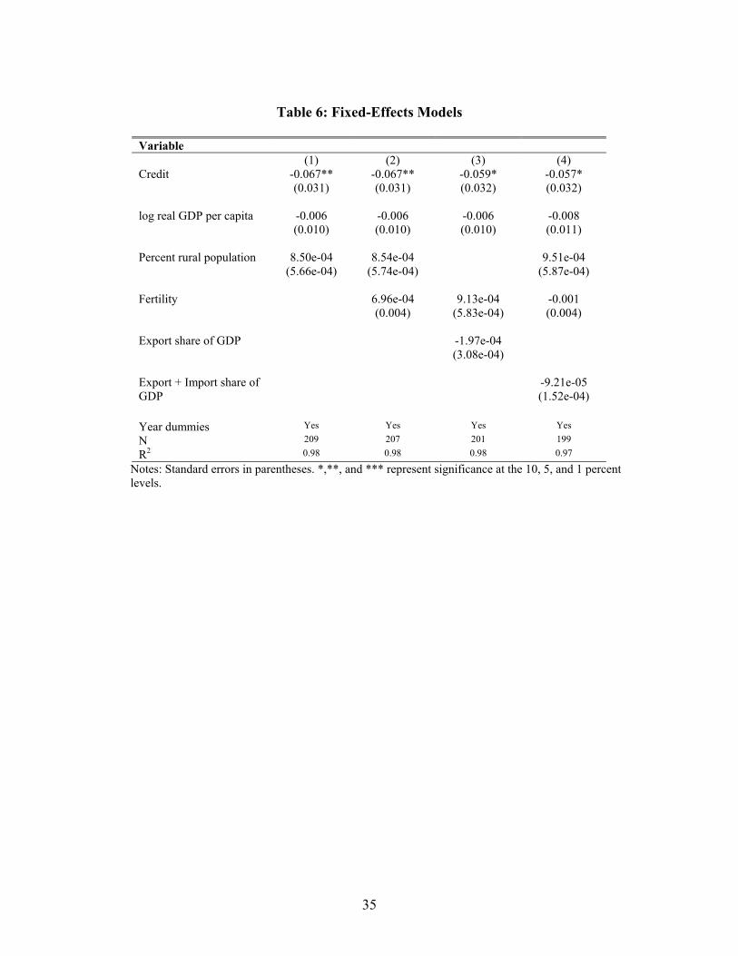
4.3 Selection on Unobservables

In this section we examine the sensitivity of our estimates to the possibility of

selection on unobservables. Because of the panel-data structure of the dataset, we can

control for selection on unobservables by including in our linear regression model fixed

effects, that allow us to control for time-invariant selection effects (Table 6). The results,

of course, remain exposed to time-varying omitted variables.

When introducing country and year fixed-effects, the magnitude of estimated

coefficient of credit smaller (column (1)). However, the effect of credit remains

significant at the 5 percent level. In contrast, the effect of log GNP per capita is now

greatly diminished in magnitude and statistical significance: it is one tenth of the OLS

estimate in Table 3, column (7). A shift from the 25th to the 75th percentile of credit

would lead to a six percent decrease in child labor, whereas the corresponding shift for

GDP per capita would lead only to a two percent decrease in child labor.

When we include additional time varying controls such as fertility, export and

export-plus-import share, and individually and simultaneously, the magnitude of the

coefficient remains similar to column (1). The fact that the level of statistical significant

decreases (to the 10% level) is not, inherently, very surprising, given that we are allowing

for country and year fixed effects for a sample of less than 80 countries with at most 5

data points each.

19

5. Conclusion

In this paper we have investigated the relationship between child labor and access to

credit across countries. The theoretical literature has highlighted the importance of this

relationship, suggesting that, in presence of credit constraints, (inefficiently high) child

labor might arise whenever parents are prevented from trading off resources

intertemporally. Our empirical results confirm the existence of a significant association

between child labor and the share of private credit issued by banks to GDP, which we

interpret as a proxy of access to credit. This relationship is particularly large, robust, and

significant in the sample of poor countries, which have both less developed financial

markets and greater child labor and, as such, are of greater policy interest. We also

provide evidence that strong financial markets dampen the impact of income variability

on child labor, which would otherwise be sizeable.

As with most work on cross-country data, caution must be used in interpreting the

estimated coefficients causally. There are many potential sources of spurious correlation

and selection. We subjected our result to a wide array of robustness checks, including

adding a range of controls (linear and squared income, share of rural population,

continent dummies, fertility, primary and secondary school enrollment, import and

exports shares, and ratification of the 1973 ILO convention on child labor), and

considering fixed effects. The relationship remains strong under all of these alternatives.

These results are important for two reasons. First, they lend empirical support to

the recent strand of the theoretical literature that highlights the role of credit constraints in

determining child labor. Second, they open an important policy window on alleviating the

problem of child labor. In this context, increasing household access to credit can be an

effective tool in reducing the extent of child labor, and has distinct advantages over other

remedies. Compared to legal restrictions and direct bans, it can decrease child labor

without lowering household welfare, and it is arguably simpler and can have a more

immediate impact than general economic development.

20

REFERENCES

Ashagrie, Kebebew (1993). “Statistics on Child Labor,” Bulletin of Labor Statistics, No.

3. Geneva: International Labor Organization.

Baland, Jean-Marie, and James Robinson (2000). “Is Child Labor Inefficient?,” Journal

of Political Economy, 108, 663-679.

Basu, Kaushik (1999). “Child Labor: Cause, Consequence, and Cure with Remarks on

International Labor Standards,” Journal of Economic Literature, 37, 1083-1119.

Beck, Thorsten, Asli Demirguc-Kunt and Ross Levine (1999). “A New Database on

Financial Development and Structure,” World Bank Policy Research Paper No. 2146.

Beck, Thorsten, Asli Demirguc-Kunt and Vojislav Maksimov (2002). “Financing

Patterns around the World; the Role of Institutions,” mimeo., The World Bank.

Becker, Gary (1964). Human Capital, New York: Columbia University Press.

--------- (1974). “A Theory of Social Interactions,” Journal of Political Economy, 82,

1063-93.

--------- and Kevin Murphy (1988). “The Family and the State,” Journal of Law and

Economics, 31, 1-18.

Beegle, Kathleen, Rajeev Dehejia, and Roberta Gatti (2002). “Do Households Resort to

Child Labor to Cope with Income Shocks?” Columbia University Working Paper No.

0203-12.

Bhagwati, Jagdish (1995). “Trade Liberalization and ‘Fair Trade’ Demands: Addressing

the Environment and Labor Standards Issues,” World Economy, 18, 745-759.

21

Bourguignon, Francois, and Pierre-Andre Chiappori (1994). “The Collective Approach to

Household Behavior,” in The Measurement of Household Welfare, Richard Blundell, Ian

Preston, and Ian Walker, eds. Cambridge: Cambridge University Press.

Brown, Drusilla, Alan Deardorff, and Robert Stern (2001). “Child Labor: Theory,

Evidence, and Policy,” School of Public Policy Discussion Paper No. 474, University of

Michigan.

Canagarajah, Roy and Harold Coulombe (1997). “Child Labor and Schooling in Ghana,”

Human Development Technical Report (Africa Region), The World Bank, Washington.

Central Intelligence Unit. The World Factbook 1995-96. Washington: Brassey’s.

Cigno, Alessandro, Furio Rosati and Lorenzo Guarcello (2002). “Does Globalization

Increase Child Labor?,” World Development, 30, 1579-1589.

Collingsworth, Terry, William Goold, and Pharis Harvey (1994). “Time for a New

Global Deal,” Foreign Affairs, 73, 8-13.

Deininger, Klaus and Lyn Squire (1996). “A New Dataset Measuring Income Inequality,”

World Bank Economic Review, 10, 565-91.

Edmonds, Eric and Nina Pavcnik (2001). “Does Globalization Increase Child Labor?

Evidence from Vietnam,” Manuscript, Dartmouth College.

--------- (2002). “Is Child Labor Inefficient?” Manuscript, Dartmouth College.

Flug, Karnit, Antonio Spilimbergo and Eric Wachtenheim (1999). “Investment in

Education: Do Economic Volatility and Credit Constraints Matter?” Journal of

Development Economics, 55, no. 2.

22

Galasso, Emanuela (1999). “Intra-Household Allocation and Child Labor in Indonesia,”

mimeo., Boston College.

Grootaert, Christian, and Ravi Kanbur (1995). “Child Labor: An Economic Perspective,”

International Labor Review, 134, 187-203.

--------- and Harry Patrinos (1999). The Policy Analysis of Child Labor: A Comparative

Study, New York: St. Martin’s Press.

Guarcello, Lorenzo, Fabrizia Mealli, and Furio Camillo Rosati (2002). “Household

Vulnerability and Child Labor: The Effect of Shocks, Credit Rationing and Insurance,”

Manuscript, Innocenti Research Center, UNICEF.

Gupta, Manash (1998). “Wage Determination of a Child Worker: A Theoretical

Analysis,” forthcoming Review of Development Economics.

Hadi, Ali (1992). “Identifying Multiple Outliers in Multivariate Data,” Journal of the

Royal Statistical Society. Series B, 54, 761-771.

ILO (1996). Economically Active Population: Estimates and Projections, 1950-2010.

Geneva.

Jacoby, Hanan (1994). “Borrowing Constraints and Progress Through School: Evidence

from Peru,” Review of Economics and Statistics, 76, 151-160.

---------, and Emmanuel Skoufias (1997). “Risk, Financial Markets, and Human Capital

in a Developing Country,” Review of Economic Studies, 64, 311-335.

King, Robert, and Ross Levine (1993). “Finance and Growth: Schumpeter Might Be

Right,” American Economics Review, 108, 717-737.

23

Krueger, Alan (1996). “Observations on International Labor Standards and Trade,”

National Bureau of Economic Research, Working Paper No. 5632.

La Porta, Rafael, Florencio Lopez-de-Silanes, Andrei Shleifer, and Robert Vishny

(1998). “The Quality of Government,” Journal of Law, Economics, and Organization,

15, 222-279.

Moehling, Carolyn (1995). “The Intra-household Allocation of Resources and the

Participation of Children in Household Decision-Making: Evidence from Early Twentieth

Century America,” Manuscript, Northwestern University.

Parsons, Donald, and Claudia Goldin (1989). “Parental Altruism and Self-Interest: Child

Labor Among Late Nineteenth-Century American Families,” Economic Inquiry, 24, 637-

659.

Rajan, Raghuram, and Luigi Zingales (1998). “Financial Dependence and Growth,”

American Economic Review, 88, 559-586.

Ranjan, Priya (1991). “An Economic Analysis of Child Labor,” Economics Letters, 64,

99-105.

--------- (2001). “Credit Constraints and the Phenomenon of Child Labor,” Journal of

Development Economics, vol.64.

Ravallion, M. and Q. Wodon (2000). “Does Child Labour Displace Schooling? Evidence

on Behavioral Responses to an Enrollment Subsidy,” The Economic Journal, 110, 158-

175.

Rogers, Carol and Kenneth Swinnerton (2001). “Inequality, Productivity and Child

Labor: Theory and Evidence,” Manuscript.

24

Rosati, Furio Camillo and Zafiris Tzannatos (2000). “Child Labor in Vietnam,”

Manuscript, The World Bank.

Srinivasan, T.N. (1996). “International Trade and Labor Standards from an Economic

Perspective,” in Challenges to the New World Trade Organization, Pitou van Dijck and

Gerrit Faber, eds. The Hague: Kluwer.

Summers, Robert and Heston, Alan. (1991). “The Penn World Table (Mark 5): An

Expanded Set of International Comparisons, 1950-1988,” Quarterly Journal of

Economics, 106, 327-368.

The World Bank (2001). World Development Indicators, Washington DC.

25

APPENDIX: Data Description and Sources

CHILDLABOR Share of the active population between age 10 and 14 over total population between 10 and 14. Active population includes people who, during the reference period, performed “some work” for wage or salary, in cash or in kind. The notion of “some work” is interpreted as work for at least 1 hour during the reference period. Source: ILO.

CREDIT Private credit by deposit money banks to GDP. Source:

Beck, Demirguc-Kunt and Levine (1999). Ln(GDPPC) Natural logarithm of real GDP per capita in constant

dollars, chain Index, expressed in international prices, base 1985. Source: Summers-Heston, years 1960-1990.

RURAL Rural population, as % of total population. Source: World

Development Indicators, World Bank. SDGROW5 Standard deviation of per capita GDP growth over the

previous 5 years. SCH_PRIF Gross primary female school enrollment (%). Gross

enrollment ratio is the ratio of total enrollment, regardless of age, to the population of the age group that officially corresponds to the level of education shown. Source: World Development Indicators, World Bank.

SCH_SECF Gross secondary female school enrollment (%). Gross

enrollment ratio is the ratio of total enrollment, regardless of age, to the population of the age group that officially corresponds to the level of education shown. Source: World Development Indicators, World Bank.

FERT Fertility rate, total births per woman. Total fertility rate

represents the number of children that would be born to a woman if she were to live to the end of her childbearing years and bear children in accordance with prevailing age-specific fertility rates. Source: World Development Indicators, World Bank.

EXP Share of exports on GDP. Source: World Development

Indicators, World Bank.

26

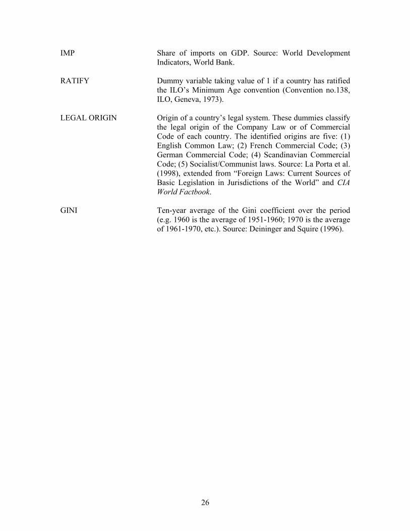
IMP Share of imports on GDP. Source: World Development Indicators, World Bank.

RATIFY Dummy variable taking value of 1 if a country has ratified

the ILO’s Minimum Age convention (Convention no.138, ILO, Geneva, 1973).

LEGAL ORIGIN Origin of a country’s legal system. These dummies classify

the legal origin of the Company Law or of Commercial Code of each country. The identified origins are five: (1) English Common Law; (2) French Commercial Code; (3) German Commercial Code; (4) Scandinavian Commercial Code; (5) Socialist/Communist laws. Source: La Porta et al. (1998), extended from “Foreign Laws: Current Sources of Basic Legislation in Jurisdictions of the World” and CIA World Factbook.

GINI Ten-year average of the Gini coefficient over the period

(e.g. 1960 is the average of 1951-1960; 1970 is the average of 1961-1970, etc.). Source: Deininger and Squire (1996).

27

Figure 1: Child Labor and Access to Credit

child

credit.00029 1.6715

0

.631

EGY MAR

PHL EGY SLV

CRI

PAK

HND

MAR

PHL ECU SLV

AUT

PRY PHL

IRN ECU

HND SYR

DZA

IRL

SLE

PRY

NOR GRC

CRI

NGA

PAK

BEN

GRC

PRY SLV

IRN

ZWE

EGY

BLZ VEN MYS

BLZ HUNTTO

COL

LBR

EGY PRY

GTM

TTO

CRI

IRL

ZWE

ZWE CMR

COL

PANMUS

SAU

MEX ECU

NGA

PER MYS

PAK

FRA

CMR

SDN

PER

NIC

ECU

BOL

FJI

MOZ

PAK

SAU TTO

CMR

DOM

ZAFHUN SWE ESP

HND MEX

DZA

NGA HTI

SLV

SWE

GHA

SLE

FJI PAN

AUT

MEX

CRI

BGD

ESP

ECU

PHL SYR

ISRDNK ESP

DOM

MUS

SOM

GTM

SDN

DOM GRC

CYP

ESP

GNB

GBR

SYR

MDG

NGA

FRA

CRI DNK

AUT

FJI NZL

URY FIN

ISL CHL

GTM

IDN COL

NIC

MEX

IND

HTI

COL

JAM

CMR

SWE

SLV

CAN

BOL IDN

VEN

SVK

ZAR

CHL

LBR DOM

FRA DNK

VEN

BOL

SUR ISL

THA

PRY

GTM

SYR JAM

SLE MEX

FIN

PHL

NLD NZL

TGO

HND

IRL

TGO

GBR IRN

CIV

ISLISR

SEN

HND

CHL

SEN

CAN SUR ISR

PER

IND GTM

FJI

BGD

NOR

GHA

CIV

THA

CHL

VEN

NLD

GHA

MDG

GHA

COG

CYPNOR

ARG

IRL

IND

SWE ISRISL CANDZA

MDG

KORAUS ZAF

BHS

ARG

AUS TUN

DNK

IDN

BGR JAM NZL

ESP

AUSBRB

CIV CIV

COG

BRB ZAF

IND

TUN

RWA

AUS MAR URY

LAO MAR

BOL

NIC

URY

KEN NER

URY

LAO

USANZL KOR

HTI

GRC

SDN

MYSUSA

BRA

BGD

KEN

TUR

NOR

GNQ

KEN KEN GMB

JPN

UGA

NLDKOR

UGA GMB

PER GRC GBR

RWA

MYS

DOM

TTO VEN

BWA KHM

PER

MMR

JPNJOR

LVA

PNG

PNG

BHR USA

GUY

MMR

ARG AUT

ZMB

SWE

BWA

BRB

SWZ

LKA LUX

MUS

NER

UKR

EGY

POL

MDG

ISR FINBEL FIN JAM AUS

PRT

ARG TTO

BELPOL

CAF

NER

COG

BDI

FRA

BWA

BRBMUS

HTI

BEL

URY

BDI

MRT

NLD

PRT

HRV ZAF

BOL

PRTMNG BEL FRANZLCAN

LKA JAM

DNK

GAB

CAN AUT

PAN

GMB

IDN

MWI

IRL

RWA

TUR

MRT

BRA SWZ

COG

PRTBLR

GAB

GUY LUX

ZAR TGO

NLD

MMR

LKA ISLFINSURMDA

BRA

NOR

THA

RUS EST

BDI NER

ZMB

SEN

MLI

SOM

USA

NPL

LKA PRT

LKA

SEN

BEL

NPL

CAF

DEU

SLB

MLI

GUY JOR

NPL

JPN

SLE GAB

MYS

TCD MWI

BHR SVN

SWZ

ARM USA

HTI

MLT

GAB

LUX

BFA

GUY

NAM

BTN

MLT CHE

NPL BTN

JOR

TCD

LUX CHE

SAU

LSO

ITAITA

LSO

BFA

MLT ITA JPNITA CHE

ZAR

BDI

GBRGBRJPN

LSO

SLB

THA

MLT

ETH

LUX

ETH

BHR

CHN

CHN

MMR

CHE

SGP

CHESGP

ZAR

HKG SGPSGP

ETH

PAN

SDN

BHSLBN

LBY PAN

IRQ

LTU

CYP

CYP

SDN

BHS ANT DEUDEU

CYP

DEU

PAK AFG

KAZ

IND

IRQ IRN

CZE

ETH

DEU

Chi

ld la

bor

28

Figure 2: Child labor and access to credit over time

0.190.17

0.140.12 0.11

0.20.22

0.27

0.320.34

0

0.05

0.1

0.15

0.2

0.25

0.3

0.35

0.4

1960 1970 1980 1990 1995

avg child laboravg credit

29

Figure 3: First difference in child labor vs. first difference in credit

Firstdifference ofchild labor

First difference of credit-.97832 .631542

-.153135

.196465

GBR

JPN

THA

ISR NLD

NZLAUS

CHL

ESP

NOR

CYP

BEL

ISRDEUISL

PANSWEECU

IND

PHL

ESP

AUT

IND

HTI

EGY

TTOVENTTO

GRC

BDINPL

IRN

DNKCRISAURWAKOR

GTM

LKA

MDG

FINSLV

SLV

BHSAUSITA

HND

BHR

BWA

NGA

PER

NER

ARG

IRN

NZL

CIV

EGY

GUYGRC

MMR

DOM

PRT

PRT

ZAR

PRY

PAK

ECU

SWE

DOM

CRI

GTM

IRL

DZA

GAB

DNK

COG

BDI

COL

NORIRL

SLE

SLEGHA

SWZ

URYCAN

SDN

SYR

JAM

CMR

ETH

LUXGBRBOL

SDN

KEN

FJI

VENUSA

PRY

ZAF

GAB

PER

MEXUSAMUS

HTI

DEU

ZWEJAMCAN

LKA

ISLIDNFRASUR

HND

PAK

MAR

SGPBGD

PHL

BRB

CHLLUX

FRA

CYP

PANURY

AUT

MEX

SEN

FIN

MYS

BEL

BOL

JPNMLT

MYS

CHENLD

CHE

30

Table 1: Data Description Variable Observations Mean Std. Dev. Min. Max. Child labor

860 0.15 0.17 0 0.79

Credit

482 0.28 0.25 0.00029 1.67

Standard deviation of income growth

631 0.04 0.04 0.00059 0.79

log real GDP per capita

705 7.76 1.06 5.41 10.58

Percent rural population

857 54.58 24.94 0 98.2

Share of exports of GDP

630 32.6 24.38 1.19 215.38

Share of imports of GDP

634 37.27 24.74 1.9 223.65

Primary female school enrolment

654 81.19 32.84 0.6 170.9

Secondary female school enrolment

639 43.57 35.5 0 151.3

Gini coefficient

302 39.22 10.11 19.5 62.87

31

Table 2: Correlations Among the Variables

Variable CHILD LABOR CREDIT SDGROW5 LRGDPPC RURAL EXP IMP SCH_PRIF SCH_PRIF GINI FERTILITY Child labor 1 Credit -0.46 1

Standard deviation of income growth 0.16 -0.27 1

log real GDP per capita -0.81 0.62 -0.23 1

Percent rural population 0.75 -0.45 0.13 -0.82 1

Export share of GDP -0.24 0.14 0.16 0.18 -0.27 1

Import share of GDP -0.13 0.07 0.14 0.03 -0.11 0.9 1

Primary female school enrolment -0.49 0.23 0.06 0.48 -0.34 0.15 0.08 1

Secondary female school enrolment -0.78 0.57 -0.22 0.84 -0.71 0.13 0.01 0.48 1

Gini coefficient 0.31 -0.33 0.31 -0.38 0.26 0.04 0.11 0.11 -0.46 1

Fertility 0.81 -0.5396 0.1952 -0.8433 0.6710 -0.1746 -0.0299 -0.5618 -0.8370 0.4523 1.0000

32

Table 3: Base Specification (dependent variable: child labor)

Including income variability Variables Basic with

CREDIT excluding outliers

low CREDIT

high CREDIT

Low income

High income

(1) (2) (3) (4) (5) (6) (7) (8) Credit -0.033**

(0.017) -0.044***

(0.018) -0.032* (0.018)

-0.15*** (0.056)

-0.014 (0.011)

Standard deviation of growth

0.19*** (0.073)

0.21*** (0.075)

0.016 (0.033)

log real GDP per capita

-0.32*** (0.043)

-0.40*** (0.058)

-0.44*** (0.052)

-0.40*** (0.056)

-0.27*** (0.061)

-0.48*** (0.058)

-0.037*** (0.012)

-0.006 (0.009)

log real GDP per capita2

0.019*** (0.003)

0.024*** (0.004)

0.026*** (0.003)

0.024*** (0.003)

0.017*** (0.004)

0.028*** (0.003)

Percent rural population

2.25e-04 (1.82e-04)

3.66e-04* (2.18e-04)

3.20e-04 (2.16e-04)

3.74e-04* (2.17e-04)

5.79e-04** (2.88e-04)

1.88e-04 (2.46e-04)

8.08e-04 (5.20e-04)

1.22e-04 (1.94e-04)

Child labor in 1950 0.69***

(0.030) 0.63*** (0.042)

0.62*** (0.042)

0.64*** (0.045)

0.72*** (0.035)

0.60*** (0.054)

0.74*** (0.049)

0.43*** (0.077)

Year trend -0.002***

(1.86e-04) -0.002*** (1.82e-04)

-0.002*** (1.78e-04)

-0.002*** (1.96e-04)

-0.002*** (2.04e-04)

-0.002*** (3.05e-04)

-0.002*** (2.94e-04)

-0.001*** (2.43e-04)

N 703 474 469 703 301 303 209 265 R2 0.93 0.92 0.92 0.92 0.93 0.93 0.88 0.67

Notes: Standard errors in parentheses. Standard errors are corrected for heteroscedasticity and clustering within countries. *,**, and *** represent significance at the 10, 5, and 1 percent levels.

33

Table 4: Tobit Specification (dependent variable: child labor) Including income variability Variables Basic with

CREDIT excluding outliers

low CREDIT

high CREDIT

Low income

High income

(1) (2) (3) (4) (5) (6) (7) (8) Credit -0.077***

(0.026) -0.076***

(0.026) -0.080***

(0.027) -0.14***

(0.059) -0.058***

(0.022) Standard deviation of growth

0.20*** (0.074)

0.19*** (0.077)

0.069* (0.038)

log real GDP per capita

-0.17*** (0.042)

-0.21*** (0.061)

-0.24*** (0.059)

-0.20*** (0.060)

-0.20*** (0.064)

-0.29*** (0.048)

-0.036 (0.20)

-0.030 (0.30)

log real GDP per capita2

0.008*** (0.003)

0.011*** (0.004)

0.013*** (0.004)

0.011*** (0.004)

0.012*** (0.004)

0.016*** (0.003)

Percent rural population

6.42e-05 (2.19e-04)

3.28e-04 (2.62e-04)

3.09e-04 (2.60e-04)

3.15e-04 (2.60e-04)

4.31e-04 (2.99e-04)

1.82e-04 (3.36e-04)

8.74e-04* (5.12e-04)

2.02e-04 (2.74e-04)

Child labor in 1950

0.77*** (0.028)

0.69*** (0.038)

0.69*** (0.038)

0.69*** (0.039)

0.75*** (0.036)

0.67*** (0.049)

0.75*** (0.051)

0.54*** (0.068)

Year trend -0.003***

(2.14e-04) -0.003*** (2.25e-04)

-0.003*** (2.23e-04)

-0.003*** (2.28e-04)

-0.002*** (2.17e-04)

-0.003*** (3.65e-04)

-0.002*** (2.99e-04)

-0.003*** (3.60e-04)

N 703 474 469 457 301 303 209 265 Obs. with child labor=0

152 107 104 96 21 92 4 103

Notes: Standard errors in parentheses. Standard errors are corrected for heteroscedasticity and clustering within countries. *,**, and *** represent significance at the 10, 5, and 1 percent levels. Marginal coefficients are reported for Tobit estimates.

34

Table 5: Robustness Checks (OLS, dependent variable: child labor)

(1) (2) (3) (4) (5) (6) (7) (8) (9) (10) Credit -0.13***

(0.056)

-0.13** (0.058)

-0.10** (0.051)

-0.11** (0.050)

-0.16*** (0.055)

-0.13** (0.059)

-0.13** (0.060)

-0.19*** (0.048)

-0.14*** (0.057)

-0.13** (0.056)

log real GDP per capita

-0.022 (0.016)

-0.027* (0.016)

-0.019 (0.015)

-0.028* (0.016)

-0.005 (0.015)

-0.020 (0.017)

-0.018 (0.016)

-0.041** (0.020)

-0.021 (0.016)

-0.002 (0.014)

Percent rural population

0.001* (5.65e-04)

8.34e-04 (6.08e-04)

0.001** (5.30e-04)

9.71e-04* (5.40e-04)

0.002*** (4.87e-

04)

0.001* (5.82e-04)

0.001** (5.75e-04)

0.001* (5.25e-04)

0.001* (5.58e-

04)

0.002*** (4.88e-04)

Child labor in 1950

0.71*** (0.049)

0.68*** (0.059)

0.67*** (0.046)

0.66*** (0.054)

0.67*** (0.052)

0.71*** (0.051)

0.71*** (0.052)

0.66*** (0.057)

0.71*** (0.051)

0.64*** (0.049)

Primary female school

-2.31e-04 (2.65e-04)

-1.72e-04 (2.64e-04)

Secondary female school

-2.58e-04 (3.13e-04)

9.84e-05 (3.62e-04)

Fertility 0.011*** (0.005)

0.013** (0.006)

0.012*** (0.005)

Export share of GDP

-1.38e-04 (2.61e-04)

-2.52e-04 (4.14e-04)

Export + Import share of GDP

-1.40e-04 (1.71e-04)

Gini coefficient -0.002*** (8.59e-04)

Ratified ILO Convention

0.011 (0.011)

0.011 (0.011)

Region dummies

yes yes yes yes yes yes yes yes yes yes

Year dummies yes yes yes yes yes yes yes yes yes yes Legal origin dummies

no no no no yes no no no no yes

N 209 175 207 174 209 201 201 84 201 199 R2 0.90 0.91 0.8979 0.91 0.90 0.89 0.89 0.89 0.91 0.90

Notes: Standard errors in parentheses. Standard errors are corrected for heteroscedasticity and clustering within countries. *,**, and *** represent significance at the 10, 5, and 1 percent levels.

35

Table 6: Fixed-Effects Models

Variable (1) (2) (3) (4) Credit -0.067**

(0.031) -0.067** (0.031)

-0.059* (0.032)

-0.057* (0.032)

log real GDP per capita -0.006

(0.010) -0.006 (0.010)

-0.006 (0.010)

-0.008 (0.011)

Percent rural population 8.50e-04

(5.66e-04) 8.54e-04

(5.74e-04) 9.51e-04

(5.87e-04) Fertility 6.96e-04

(0.004) 9.13e-04

(5.83e-04) -0.001 (0.004)

Export share of GDP -1.97e-04

(3.08e-04)

Export + Import share of GDP

-9.21e-05 (1.52e-04)

Year dummies Yes Yes Yes Yes

N 209 207 201 199

R2 0.98 0.98 0.98 0.97

Notes: Standard errors in parentheses. *,**, and *** represent significance at the 10, 5, and 1 percent levels.