Reusable Software Infrastructure for

Stream Processing

by

Robert Soule

A dissertation submitted in partial fulfillment

of the requirements for the degree of

Doctor of Philosophy

Department of Computer Science

Courant Institute of Mathematical Sciences

New York University

May 2012

Professor Robert Grimm

c© Robert Soule

All Rights Reserved, 2012

Abstract

Developers increasingly use streaming languages to write their data processing applications. While

a variety of streaming languages exist, each targeting a particular application domain, they are all

similar in that they represent a program as a graph of streams (i.e. sequences of data items) and

operators (i.e. data transformers). They are also similar in that they must process large volumes

of data with high throughput. To meet this requirement, compilers of streaming languages must

provide a variety of streaming-specific optimizations, including automatic parallelization. Tradi-

tionally, when many languages share a set of optimizations, language implementors translate the

source languages into a common representation called an intermediate language (IL). Because

optimizations can modify the IL directly, they can be re-used by all of the source languages,

reducing the overall engineering effort. However, traditional ILs and their associated optimiza-

tions target single-machine, single-process programs. In contrast, the kinds of optimizations that

compilers must perform in the streaming domain are quite different, and often involve reasoning

across multiple machines. Consequently, existing ILs are not suited to streaming languages.

This thesis addresses the problem of how to provide a reusable infrastructure for stream pro-

cessing languages. Central to the approach is the design of an intermediate language specifically

for streaming languages and optimizations. The hypothesis is that an intermediate language

designed to meet the requirements of stream processing can assure implementation correctness;

reduce overall implementation effort; and serve as a common substrate for critical optimizations.

In evidence, this thesis provides the following contributions: (1) a catalog of common streaming

optimizations that helps define the requirements of a streaming IL; (2) a calculus that enables

reasoning about the correctness of source language translation and streaming optimizations; and

(3) an intermediate language that preserves the semantics of the calculus, while addressing the

implementation issues omitted from the calculus. This work significantly reduces the effort it

takes to develop stream processing languages by making optimizations reusable across languages,

and jump-starts innovation in language and optimization design.

iii

Acknowledgments

First, and foremost, I would like to thank my advisor, Robert Grimm. I have been very fortunate

to work with Robert since I was a master’s student, and it is largely based on his encouragement

and support that I pursued my doctoral degree. Robert has a remarkable ability to distill

our research into succinct points, a tireless commitment to clarity, and an annoying knack for

(usually) being right. He not only always expects the best from me, but taught me to expect the

best from myself. I will always be grateful for his guidance and friendship.

I would like to thank Martin Hirzel, who has been my co-advisor for the past several years.

Martin is a fantastic researcher, and a dedicated mentor. He was always available when I needed

help, and has an amazing capacity to articulate complex ideas clearly. I greatly appreciate the

incredible amount of time and effort that Martin put into my development as a researcher, as

well as his unending patience.

Saman Amarasinghe supported me as a visiting student at MIT during the summer of 2011,

and has continued to mentor me over the past year. I wish to thank him for the wonderful

opportunity to learn from him, and for agreeing to serve on my thesis committee. I am also

obliged to my additional committee members: Jinyang Li and Benjamin Goldberg.

It has been my pleasure to work with Michael Gordon. I appreciate Mike’s vast experience

with stream processing, as well as unparalleled ability to roast a leg of lamb.

This thesis focuses on language support for distributed stream processing. I was introduced to

streaming during my internship at IBM Research, and my interest grew during my two and half

years spent as a co-op working with the System S team. This thesis would not have been possible

without my co-authors: Henrique Andrade, Bugra Gedik, Vibhore Kumar, Scott Schneider,

Huayong Wang, Kun-Lung Wu, and Qiong Zou. I would particularly like to thank Bugra for

sharing his experience with System S, and for serving on my thesis proposal committee. John

Field, Yoonho Park, Rodric Rabbah, and Martin Vechev provided me with invaluable feedback on

early versions of this work. I would also like to thank Nagui Halim for giving me the opportunity

to work with such a talented group of people, as well as for his encouragement of my research.

iv

I would like to express my gratitude to my other collaborators during my time in graduate

school. I greatly enjoyed working with Nalini Belaramani, Mike Dahlin, and Petros Maniatis. I

would like to give a special thanks to Nikolaos Michalakis, my co-author and office-mate during

my first years of school. And, of course, Leslie Cerve, without whom nothing would get done on

the 7th floor of 719 Broadway.

I would like to thank my family: my mom, my grandma, aunt Nilda, and mother-in-law Agda

for their love and support. Thank you to the Antonio family: Peter, Deli, Jonathan, and Julia

for being so understanding when I missed countless birthday parties and barbecues because I

was working.

Finally, I dedicate this thesis to my wife, Susie, for encouraging me to pursue my dreams, for

always offering a sympathetic ear, and for providing a constant source of love. And, of course,

to our two babies on the way, who are adding extra inspiration to finish!

v

Table of Contents

Abstract iii

Acknowledgments iv

List of Figures xiii

List of Tables xiv

1 Introduction 1

1.1 This Dissertation . . . . . . . . . . . . . . . . . . . . . . . . . . . . . . . . . . . . 2

1.2 Evaluation . . . . . . . . . . . . . . . . . . . . . . . . . . . . . . . . . . . . . . . . 4

1.3 Research Contributions . . . . . . . . . . . . . . . . . . . . . . . . . . . . . . . . 5

2 Stream Processing Optimizations 6

2.0.1 Background . . . . . . . . . . . . . . . . . . . . . . . . . . . . . . . . . . . 8

2.1 Operator Reordering (a.k.a. hoisting, sinking, rotation, pushdown) . . . . . . . . . . . . 10

2.1.1 Example . . . . . . . . . . . . . . . . . . . . . . . . . . . . . . . . . . . . . 10

2.1.2 Profitability . . . . . . . . . . . . . . . . . . . . . . . . . . . . . . . . . . . 10

2.1.3 Safety . . . . . . . . . . . . . . . . . . . . . . . . . . . . . . . . . . . . . . 11

2.1.4 Variations . . . . . . . . . . . . . . . . . . . . . . . . . . . . . . . . . . . . 11

2.1.5 Dynamism . . . . . . . . . . . . . . . . . . . . . . . . . . . . . . . . . . . 13

2.2 Redundancy Elimination (a.k.a. subgraph sharing, multi-query optimization) . . . . . . . 13

2.2.1 Example . . . . . . . . . . . . . . . . . . . . . . . . . . . . . . . . . . . . . 13

2.2.2 Profitability . . . . . . . . . . . . . . . . . . . . . . . . . . . . . . . . . . . 14

2.2.3 Safety . . . . . . . . . . . . . . . . . . . . . . . . . . . . . . . . . . . . . . 14

2.2.4 Variations . . . . . . . . . . . . . . . . . . . . . . . . . . . . . . . . . . . . 15

2.2.5 Dynamism . . . . . . . . . . . . . . . . . . . . . . . . . . . . . . . . . . . 16

2.3 Operator Separation (a.k.a. decoupled software pipelining) . . . . . . . . . . . . . . . . 16

vi

2.3.1 Example . . . . . . . . . . . . . . . . . . . . . . . . . . . . . . . . . . . . . 16

2.3.2 Profitability . . . . . . . . . . . . . . . . . . . . . . . . . . . . . . . . . . . 17

2.3.3 Safety . . . . . . . . . . . . . . . . . . . . . . . . . . . . . . . . . . . . . . 17

2.3.4 Variations . . . . . . . . . . . . . . . . . . . . . . . . . . . . . . . . . . . . 18

2.3.5 Dynamism . . . . . . . . . . . . . . . . . . . . . . . . . . . . . . . . . . . 19

2.4 Fusion (a.k.a. superbox scheduling) . . . . . . . . . . . . . . . . . . . . . . . . . . . . 19

2.4.1 Example . . . . . . . . . . . . . . . . . . . . . . . . . . . . . . . . . . . . . 19

2.4.2 Profitability . . . . . . . . . . . . . . . . . . . . . . . . . . . . . . . . . . . 19

2.4.3 Safety . . . . . . . . . . . . . . . . . . . . . . . . . . . . . . . . . . . . . . 20

2.4.4 Variations . . . . . . . . . . . . . . . . . . . . . . . . . . . . . . . . . . . . 20

2.4.5 Dynamism . . . . . . . . . . . . . . . . . . . . . . . . . . . . . . . . . . . 21

2.5 Fission (a.k.a. partitioning, data parallelism, replication) . . . . . . . . . . . . . . . . . . 22

2.5.1 Example . . . . . . . . . . . . . . . . . . . . . . . . . . . . . . . . . . . . . 22

2.5.2 Profitability . . . . . . . . . . . . . . . . . . . . . . . . . . . . . . . . . . . 22

2.5.3 Safety . . . . . . . . . . . . . . . . . . . . . . . . . . . . . . . . . . . . . . 23

2.5.4 Variations . . . . . . . . . . . . . . . . . . . . . . . . . . . . . . . . . . . . 24

2.5.5 Dynamism . . . . . . . . . . . . . . . . . . . . . . . . . . . . . . . . . . . 25

2.6 Placement (a.k.a. layout) . . . . . . . . . . . . . . . . . . . . . . . . . . . . . . . . . 25

2.6.1 Example . . . . . . . . . . . . . . . . . . . . . . . . . . . . . . . . . . . . . 25

2.6.2 Profitability . . . . . . . . . . . . . . . . . . . . . . . . . . . . . . . . . . . 26

2.6.3 Safety . . . . . . . . . . . . . . . . . . . . . . . . . . . . . . . . . . . . . . 27

2.6.4 Variations . . . . . . . . . . . . . . . . . . . . . . . . . . . . . . . . . . . . 27

2.6.5 Dynamism . . . . . . . . . . . . . . . . . . . . . . . . . . . . . . . . . . . 28

2.7 Load Balancing . . . . . . . . . . . . . . . . . . . . . . . . . . . . . . . . . . . . . 28

2.7.1 Example . . . . . . . . . . . . . . . . . . . . . . . . . . . . . . . . . . . . . 28

2.7.2 Profitability . . . . . . . . . . . . . . . . . . . . . . . . . . . . . . . . . . . 29

2.7.3 Safety . . . . . . . . . . . . . . . . . . . . . . . . . . . . . . . . . . . . . . 29

2.7.4 Variations . . . . . . . . . . . . . . . . . . . . . . . . . . . . . . . . . . . . 30

vii

2.7.5 Dynamism . . . . . . . . . . . . . . . . . . . . . . . . . . . . . . . . . . . 31

2.8 State Sharing (a.k.a. synopsis sharing, double-buffering) . . . . . . . . . . . . . . . . . . 31

2.8.1 Example . . . . . . . . . . . . . . . . . . . . . . . . . . . . . . . . . . . . . 31

2.8.2 Profitability . . . . . . . . . . . . . . . . . . . . . . . . . . . . . . . . . . . 31

2.8.3 Safety . . . . . . . . . . . . . . . . . . . . . . . . . . . . . . . . . . . . . . 32

2.8.4 Variations . . . . . . . . . . . . . . . . . . . . . . . . . . . . . . . . . . . . 32

2.8.5 Dynamism . . . . . . . . . . . . . . . . . . . . . . . . . . . . . . . . . . . 33

2.9 Batching (a.k.a. train scheduling, execution scaling) . . . . . . . . . . . . . . . . . . . . 34

2.9.1 Example . . . . . . . . . . . . . . . . . . . . . . . . . . . . . . . . . . . . . 34

2.9.2 Profitability . . . . . . . . . . . . . . . . . . . . . . . . . . . . . . . . . . . 34

2.9.3 Safety . . . . . . . . . . . . . . . . . . . . . . . . . . . . . . . . . . . . . . 35

2.9.4 Variations . . . . . . . . . . . . . . . . . . . . . . . . . . . . . . . . . . . . 35

2.9.5 Dynamism . . . . . . . . . . . . . . . . . . . . . . . . . . . . . . . . . . . 36

2.10 Algorithm Selection (a.k.a. translation to physical query plan) . . . . . . . . . . . . . . 36

2.10.1 Example . . . . . . . . . . . . . . . . . . . . . . . . . . . . . . . . . . . . . 36

2.10.2 Profitability . . . . . . . . . . . . . . . . . . . . . . . . . . . . . . . . . . . 36

2.10.3 Safety . . . . . . . . . . . . . . . . . . . . . . . . . . . . . . . . . . . . . . 37

2.10.4 Variations . . . . . . . . . . . . . . . . . . . . . . . . . . . . . . . . . . . . 37

2.10.5 Dynamism . . . . . . . . . . . . . . . . . . . . . . . . . . . . . . . . . . . 38

2.11 Load Shedding (a.k.a. admission control, graceful degradation) . . . . . . . . . . . . . . 39

2.11.1 Example . . . . . . . . . . . . . . . . . . . . . . . . . . . . . . . . . . . . . 39

2.11.2 Profitability . . . . . . . . . . . . . . . . . . . . . . . . . . . . . . . . . . . 39

2.11.3 Safety . . . . . . . . . . . . . . . . . . . . . . . . . . . . . . . . . . . . . . 40

2.11.4 Variations . . . . . . . . . . . . . . . . . . . . . . . . . . . . . . . . . . . . 40

2.11.5 Dynamism . . . . . . . . . . . . . . . . . . . . . . . . . . . . . . . . . . . 41

2.12 Discussion . . . . . . . . . . . . . . . . . . . . . . . . . . . . . . . . . . . . . . . . 41

2.12.1 How to specify streaming applications . . . . . . . . . . . . . . . . . . . . 41

2.12.2 How streaming optimizations enable each other . . . . . . . . . . . . . . . 43

viii

2.12.3 How streaming optimizations interact with traditional compilers . . . . . 44

2.12.4 Dynamic optimization for streaming systems . . . . . . . . . . . . . . . . 45

2.12.5 Assumptions, stated or otherwise . . . . . . . . . . . . . . . . . . . . . . . 46

2.12.6 Metrics for streaming optimization profitability . . . . . . . . . . . . . . . 47

2.13 Requirements for a Streaming IL . . . . . . . . . . . . . . . . . . . . . . . . . . . 48

2.14 Chapter Summary . . . . . . . . . . . . . . . . . . . . . . . . . . . . . . . . . . . 49

3 The Brooklet Calculus for Stream Processing 50

3.1 Notation . . . . . . . . . . . . . . . . . . . . . . . . . . . . . . . . . . . . . . . . . 52

3.2 Brooklet . . . . . . . . . . . . . . . . . . . . . . . . . . . . . . . . . . . . . . . . . 52

3.2.1 Brooklet Program Example: IBM Market Maker . . . . . . . . . . . . . . 53

3.2.2 Brooklet Syntax . . . . . . . . . . . . . . . . . . . . . . . . . . . . . . . . 53

3.2.3 Brooklet Semantics . . . . . . . . . . . . . . . . . . . . . . . . . . . . . . . 54

3.2.4 Brooklet Execution Function . . . . . . . . . . . . . . . . . . . . . . . . . 56

3.2.5 Brooklet Summary . . . . . . . . . . . . . . . . . . . . . . . . . . . . . . . 57

3.3 Language Mappings . . . . . . . . . . . . . . . . . . . . . . . . . . . . . . . . . . 57

3.3.1 CQL and Stream-Relational Algebra . . . . . . . . . . . . . . . . . . . . . 57

3.3.2 StreamIt and Synchronous Data Flow . . . . . . . . . . . . . . . . . . . . 62

3.3.3 Sawzall and MapReduce . . . . . . . . . . . . . . . . . . . . . . . . . . . . 66

3.3.4 Translation Correctness . . . . . . . . . . . . . . . . . . . . . . . . . . . . 70

3.4 Optimizations . . . . . . . . . . . . . . . . . . . . . . . . . . . . . . . . . . . . . . 70

3.4.1 Operator Fission . . . . . . . . . . . . . . . . . . . . . . . . . . . . . . . . 70

3.4.2 Operator Fusion . . . . . . . . . . . . . . . . . . . . . . . . . . . . . . . . 72

3.4.3 Reordering of Operators . . . . . . . . . . . . . . . . . . . . . . . . . . . . 73

3.4.4 Optimizations Summary . . . . . . . . . . . . . . . . . . . . . . . . . . . . 75

3.5 Chapter Summary . . . . . . . . . . . . . . . . . . . . . . . . . . . . . . . . . . . 75

4 From a Calculus to an Intermediate Language for Stream Processing 76

4.1 Maintaining Properties of the Calculus . . . . . . . . . . . . . . . . . . . . . . . . 77

ix

4.1.1 Brooklet Abstractions and their Rationale . . . . . . . . . . . . . . . . . . 77

4.1.2 River Concretizations and their Rationale . . . . . . . . . . . . . . . . . . 78

4.1.3 Maximizing Concurrency while Upholding Atomicity . . . . . . . . . . . . 80

4.1.4 Bounding Queue Sizes . . . . . . . . . . . . . . . . . . . . . . . . . . . . . 81

4.2 Making Language Development Economic . . . . . . . . . . . . . . . . . . . . . . 83

4.2.1 Brooklet Treatment of Source Languages . . . . . . . . . . . . . . . . . . 83

4.2.2 River Implementation of Source Languages . . . . . . . . . . . . . . . . . 85

4.2.3 River Translation Source . . . . . . . . . . . . . . . . . . . . . . . . . . . 86

4.2.4 River Translation Target . . . . . . . . . . . . . . . . . . . . . . . . . . . . 87

4.2.5 River Translation Specification . . . . . . . . . . . . . . . . . . . . . . . . 88

4.3 Safe and Portable Optimizations . . . . . . . . . . . . . . . . . . . . . . . . . . . 90

4.3.1 Brooklet Treatment of Optimizations . . . . . . . . . . . . . . . . . . . . . 90

4.3.2 River Optimization Support . . . . . . . . . . . . . . . . . . . . . . . . . . 91

4.3.3 Fusion Optimizer . . . . . . . . . . . . . . . . . . . . . . . . . . . . . . . . 92

4.3.4 Fission Optimizer . . . . . . . . . . . . . . . . . . . . . . . . . . . . . . . 93

4.3.5 Placement Optimizer . . . . . . . . . . . . . . . . . . . . . . . . . . . . . . 95

4.3.6 When to Optimize . . . . . . . . . . . . . . . . . . . . . . . . . . . . . . . 96

4.4 Runtime Support . . . . . . . . . . . . . . . . . . . . . . . . . . . . . . . . . . . . 97

4.4.1 Streaming Runtime . . . . . . . . . . . . . . . . . . . . . . . . . . . . . . . 98

4.4.2 Runtime Adaptation . . . . . . . . . . . . . . . . . . . . . . . . . . . . . . 98

4.4.3 Variables and Operators . . . . . . . . . . . . . . . . . . . . . . . . . . . . 99

4.5 Evaluation . . . . . . . . . . . . . . . . . . . . . . . . . . . . . . . . . . . . . . . . 100

4.5.1 Support for Existing Languages . . . . . . . . . . . . . . . . . . . . . . . . 100

4.5.2 Suitability for Optimizations . . . . . . . . . . . . . . . . . . . . . . . . . 102

4.5.3 Concurrency . . . . . . . . . . . . . . . . . . . . . . . . . . . . . . . . . . 105

4.6 Chapter Summary . . . . . . . . . . . . . . . . . . . . . . . . . . . . . . . . . . . 107

5 Related Work 108

5.1 Streaming Languages . . . . . . . . . . . . . . . . . . . . . . . . . . . . . . . . . . 108

x

5.2 Surveys on Stream Processing . . . . . . . . . . . . . . . . . . . . . . . . . . . . . 108

5.3 Semantics of Stream Processing . . . . . . . . . . . . . . . . . . . . . . . . . . . . 108

5.4 Continuous Queries . . . . . . . . . . . . . . . . . . . . . . . . . . . . . . . . . . . 109

5.5 Intermediate Language for Streaming . . . . . . . . . . . . . . . . . . . . . . . . . 109

5.6 Economic Source-Language Development . . . . . . . . . . . . . . . . . . . . . . 110

5.7 Streaming Optimizations . . . . . . . . . . . . . . . . . . . . . . . . . . . . . . . . 110

6 Limitations and Future Work 112

7 Conclusion 115

Bibliography 130

Appendices 131

A CQL Translation Correctness 132

A.1 Background on CQL Formal Semantics . . . . . . . . . . . . . . . . . . . . . . . . 132

A.1.1 CQL Function Environment. . . . . . . . . . . . . . . . . . . . . . . . . . 132

A.1.2 CQL Execution Semantics Function. . . . . . . . . . . . . . . . . . . . . . 134

A.1.3 CQL Input and Output Translation. . . . . . . . . . . . . . . . . . . . . . 135

A.2 CQL Main Theorem and Proof . . . . . . . . . . . . . . . . . . . . . . . . . . . . 137

A.3 Detailed Inductive Proof of CQL Correctness . . . . . . . . . . . . . . . . . . . . 138

B StreamIt Mapping Details 147

C StreamIt Translation Correctness 150

C.1 Background on StreamIt Formal Semantics . . . . . . . . . . . . . . . . . . . . . 150

C.1.1 StreamIt Function Environment. . . . . . . . . . . . . . . . . . . . . . . . 150

C.1.2 StreamIt Intermediate Algebra. . . . . . . . . . . . . . . . . . . . . . . . . 151

C.1.3 StreamIt Execution Semantics Function. . . . . . . . . . . . . . . . . . . . 153

C.1.4 StreamIt Input and Output Translation. . . . . . . . . . . . . . . . . . . . 156

C.2 StreamIt Main Theorem and Proof . . . . . . . . . . . . . . . . . . . . . . . . . . 157

xi

C.3 Detailed Inductive Proof of StreamIt Correctness . . . . . . . . . . . . . . . . . . 158

D Data Parallelism Optimization Correctness 161

E Fusion Optimization Correctness 162

F Selection Hoisting Optimization Correctness 163

xii

List of Figures

2.1 Pipeline, task, and data parallelism in stream graphs. . . . . . . . . . . . . . . . 9

2.2 Interactions of streaming optimizations. . . . . . . . . . . . . . . . . . . . . . . . 43

3.1 Brooklet syntax and semantics. . . . . . . . . . . . . . . . . . . . . . . . . . . . . 53

3.2 CQL semantics on Brooklet. . . . . . . . . . . . . . . . . . . . . . . . . . . . . . . 58

3.3 StreamIt round-robin split and join semantics on Brooklet. . . . . . . . . . . . . 65

3.4 Sawzall semantics on Brooklet. . . . . . . . . . . . . . . . . . . . . . . . . . . . . 66

4.1 Algorithm for assigning shared variables to equivalence classes. . . . . . . . . . . 81

4.2 Algorithm for implementing back-pressure. . . . . . . . . . . . . . . . . . . . . . 82

4.3 Example source code in original languages and their River dialects. . . . . . . . . 84

4.4 Stack of layers for executing River. . . . . . . . . . . . . . . . . . . . . . . . . . . 97

4.5 Structural view for the CQL and StreamIt benchmarks in River. . . . . . . . . . 100

4.6 Speedup and scaleup of benchmarks after optimization in River. . . . . . . . . . 103

4.7 River locking experiments . . . . . . . . . . . . . . . . . . . . . . . . . . . . . . . 106

A.1 CQL input and output translation. . . . . . . . . . . . . . . . . . . . . . . . . . . 136

A.2 CQL translation correctness, structural induction base. . . . . . . . . . . . . . . . 137

A.3 CQL translation correctness, structural induction step. . . . . . . . . . . . . . . . 142

C.1 StreamIt index transforms for a filter. . . . . . . . . . . . . . . . . . . . . . . . . 154

C.2 StreamIt index transforms for a split-join. . . . . . . . . . . . . . . . . . . . . . . 155

C.3 StreamIt input and output translation. . . . . . . . . . . . . . . . . . . . . . . . . 156

C.4 StreamIt translation correctness. . . . . . . . . . . . . . . . . . . . . . . . . . . . 157

xiii

List of Tables

2.1 The optimizations cataloged in this survey. . . . . . . . . . . . . . . . . . . . . . 7

xiv

1

Introduction

Stream processing applications are everywhere. In entertainment, people increasingly consume

music and movies as streaming media through internet services such as Spotify and Netflix.

Netflix alone accounts for nearly 30% of downstream internet traffic during peak hours [98]. In

finance, high-frequency trading programs federate live data feeds from independent exchanges to

complete transactions. Indeed, high-frequency trading accounts for 50–60% of all trades in the

United States [75]. In healthcare, streaming systems monitor patients to predict the onset of

critical situations, allowing doctors to quickly respond to life-threatening events. In the neonatal

intensive care unit, streaming systems can predict the onset of sepsis in premature babies 24

hours sooner than experienced ICU nurses [58].

Stream processing sits at the intersection of two converging trends. First, as the amount of

digital information grows [2], there is a greater demand for data-centric applications. Second, as

multicore machines and cluster computing become commonplace [1], applications are expected to

utilize available resources by running on multiple processors or multiple machines. These trends

have resulted in a paradigm shift that has a profound impact on the design of both programming

languages and optimizations.

First, to encourage (and enforce) this new paradigm, stream processing languages represent

an application as a data-flow graph of streams and operators, where each stream is an infinite

sequence of data items, and each operator transforms data. A growing body of research explores,

from the language design perspective, how to best build streaming applications [8, 11, 19, 25,

27, 28, 42, 54, 73, 77, 84, 93, 112, 123]. These languages tend to be tailored to specific classes of

applications, for example, by building on relational algebra to filter, project, join, and aggregate

streams of records (CQL [8]), or designed to support certain optimizations, such as by enforcing

static data transfer to enable double-buffering and operator fission (StreamIt [112]).

Second, while traditional compiler optimizations, such as function inlining, loop invariant

code motion, and register allocation, seek to improve performance on a single process or machine,

stream processing optimizations aim to maximize resource utilization on large multi-processors

1

and clusters of workstations, often by rewriting an application’s dataflow graph [7, 10, 12, 14,

18, 20, 23, 25, 32, 42, 45, 46, 57, 63, 73, 92, 95, 99, 101, 103, 102, 108, 116, 117, 119, 122].

Examples of important streaming optimizations include operator placement, fusion, and fission

(or replication), which are all implemented in Sawzall [93] and the cluster back-end for StreamIt

[112]. Non-distributed streaming languages, such as CQL [8], will need to implement these core

optimizations if they expect to scale with increased workloads.

To continue to advance the state of the art for both languages and optimizations, language

implementors need the proper infrastructure. An intermediate language (IL) provides a platform-

independent target for source language translation. There are several notable examples of com-

pilers or virtual machines that use ILs to decouple source languages from the target platform,

including SUIF [5] the JVM [72], and the CLR [52]. This decoupling improves source language

portability, and reduces engineering effort by providing a common substrate for optimization.

Unfortunately, because streaming optimizations involve reasoning about an entire distributed

application, existing ILs are ill-suited for stream processing languages. Given the lack of an

appropriate IL, language designers have been forced to use make-shift solutions. For example,

several languages [24, 44, 88] , somewhat surprisingly, utilize MapReduce [29] as an intermedi-

ate language. However, MapReduce is limited in that it supports only batch processing, not

continuous streaming. Alternatively, Dryad [60] provides a more general execution model than

MapReduce’s two-phased execution, but still supports only batch processing. The reality is that

an intermediate language for stream processing does not exist.

1.1 This Dissertation

This thesis addresses the problem of how to provide a reusable infrastructure for stream processing

languages. Central to the approach is the design of an intermediate language specifically for

streaming languages and optimizations. The hypothesis is that an intermediate language

designed to meet the requirements of stream processing can serve as a common

substrate for critical optimizations; assure implementation correctness; and reduce

overall implementation effort. There are three components to this work that support the

2

hypothesis.

First, this thesis systematically explores the requirements for stream processing by creating

a catalog of common streaming optimizations (§ 2). There is an abundance of prior work on

streaming optimizations. The problem is that many different research communities have in-

dependently arrived at stream processing as a programming model for high-performance and

parallel computation, including digital signal processing, databases, operating systems, and com-

plex event processing. As a result, each of these communities has developed some of the same

optimizations, but often with conflicting terminology and unstated assumptions. This catalog

both consolidates terminology and makes assumptions explicit. In the process, it clarifies what

information a streaming IL needs to provide in order to support streaming optimizations.

Second, the requirements inform the design of the Brooklet calculus for stream processing

(§ 3). Brooklet defines a core minimal language that can represent a diverse set of streaming

languages, and allows us to reason about the correctness of optimizations. To facilitate that

reasoning, it makes explicit those things that require special machinery in distributed systems.

It has a small-step operational semantics, which models execution as a sequence of atomic oper-

ator firings. It does not, however, define the order of the firings. The non-deterministic choice

reflects the fact that ordered execution in a distributed system requires additional machinery,

such as a sequencer. All uses of state are explicit, since keeping state consistent across nodes in

a distributed system requires explicit machinery, such as two-phase commit. Finally, all commu-

nication is explicit, and one-to-one (i.e., connect an output of exactly one operator with an input

of exactly one operator), because any form of many-to-many communication in a distributed

system requires, again, explicit machinery, such as application-level multicast. This emphasis

on distributed implementation distinguishes Brooklet from prior work on stream processing se-

mantics [22, 50, 56, 62, 70, 79]. Brooklet provides a formal foundation for the design of the

IL.

Finally, this thesis presents the River intermediate language (§ 4). River builds on Brook-

let by addressing the real-world details that the calculus elides. Notably, River provides an

implementation language for operator implementations; maximizes the concurrent execution of

3

operators while preserving the sequential semantics of Brooklet; and uses back-pressure to avoid

buffer overflows in the presence of bounded queues. Because every River program can be trivially

abstracted into a Brooklet program, River is a practical intermediate language with a rigorously

defined semantics. Moreover, this thesis explores techniques for making language development

economic, through the use of modular parsers, type checkers, and code generators. The result is a

set of tools and artifacts for developing River compilers. Collectively, the River IL and associated

tools provide a reusable software infrastructure for stream processing.

1.2 Evaluation

River defines an intermediate language for stream processing based on the Brooklet calculus. We

define formal translations from three representative languages, CQL, Sawzall, and StreamIt, into

Brooklet (§ 3.3) , and proofs for the safety of three vital streaming optimizations, operator fusion,

fission, and placement, in Brooklet(§ 3.4) . Every River program can be trivially abstracted into

a Brooklet program and every River execution also is a Brooklet execution. Consequently, the IL

has a well-defined formal foundation, making it possible to rigorously reason about the correctness

of translations and optimizations.

To verify that River is able to support a diversity of streaming languages, we implemented

language translators for CQL, StreamIt, and Sawzall, as well as illustrative benchmark appli-

cations (§ 4.2). The benchmarks exercise a significant portion of each language, demonstrating

that River is expressive enough to support a wide variety of streaming languages.

To verify that River is extensible enough to support a diverse set of streaming optimizations,

we implemented three critical streaming optimizations: operator fusion, fission, and placement

that operate on the IL directly (§ 4.3). These optimizations demonstrate that River can serve a

common substrate for critical optimizations.

Finally, we wrote a back-end for River on System S [42], a high-performance distributed

streaming runtime. We then evaluated the effects of applying the three high-level optimiza-

tions to the benchmark applications written in the three different streaming languages (§ 4.5).

River effectively decouples the optimizations from the language front-ends, and thus makes them

4

reusable across front-ends. Because of this reuse, River reduces the overall implementation effort.

1.3 Research Contributions

This dissertation makes the following contributions:

1. It provides a systematic exploration of the requirements for an intermediate lan-

guage for stream processing by developing a catalog of common streaming optimiza-

tions.

2. It develops a formal foundation for the design of the intermediate language for

stream processing with a calculus that enables reasoning about the correctness of source

language translation and streaming optimizations.

3. It presents an intermediate language for stream processing with a rigorously

defined semantic that decouples language front-ends from optimizations.

4. It defines the first formal semantics for the Sawzall language as a byproduct of the

Sawzall-to-Brooklet translation.

5. It reports the first distributed implementation of CQL as a product of our CQL-to-

River translation and the River-to-System S [42] backend.

In short, this thesis provides a reusable software infrastructure for stream processing. It increases

the portability of stream processing languages, and enables the reuse of common streaming

optimizations. This work helps to support and encourage future innovation in language and

optimization design.

5

2

Stream Processing Optimizations

Streaming applications are programs that process continuous data streams. These applications

have become ubiquitous due to increased automation in telecommunications, health-care, trans-

portation, retail, science, security, emergency response, and finance. As a result, various research

communities have independently developed programming models for streaming. While there are

differences both at the language level and at the system level, each of these communities ulti-

mately represents streaming applications as a graph of streams and operators, where each stream

is a conceptually infinite sequence of data items, and each operator consumes data items from

incoming streams and produces data items on outgoing streams. Since many streaming applica-

tions require extreme performance, each community has developed a number of optimizations.

The communities that have focused the most on streaming optimizations are digital signal pro-

cessing, operating systems and networks, databases, and complex event processing. The latter

discipline, for those unfamiliar with it, uses temporal patterns over sequences of events (i.e., data

items), and reports each match as a complex event.

Unfortunately, while there is plenty of literature on streaming optimizations, the literature

uses inconsistent terminology. For instance, what we refer to as an operator is called operator in

CQL [8], filter in StreamIt [112], box in Aurora and Borealis [4, 3], stage in Seda [114], actor in

Flextream [57], and module in River [10]. As another example for inconsistent terminology, push-

down in databases and hoisting in compilers are essentially the same optimization, and therefore,

we advocate the more neutral term operator reordering. To establish common vocabulary, we

took inspiration from catalogs for design patterns [40] and for refactorings [38]. Those catalogs

have done a great service to practitioners and researchers alike by raising awareness and using

consistent terminology. This chapter is a catalog of the stream processing optimizations listed in

Table 2.1.

Besides inconsistent terminology, this chapter is further motivated by unstated assumptions:

certain communities take things for granted that other communities do not. For example, while

StreamSQL assumes that stream graphs are forests (acyclic sets of trees), StreamIt assumes

6

Table 2.1: The optimizations cataloged in this survey. Column “Graph” indicates whetheror not the optimization changes the topology of the stream graph. Column “Semantics” indi-cates whether or not the optimization changes the semantics, i.e., the input/output behavior.Column “Dynamic” indicates whether the optimization happens statically (before runtime) ordynamically (during runtime). Entries labeled “(depends)” indicate that both alternatives arewell-represented in the literature.

Section Optimization Graph Semantics Dynamic2.1. Operator reordering changed unchanged (depends)2.2. Redundancy elimination changed unchanged (depends)2.3. Operator separation changed unchanged static2.4. Fusion changed unchanged (depends)2.5. Fission changed (depends) (depends)2.6. Placement unchanged unchanged (depends)2.7. Load balancing unchanged unchanged (depends)2.8. State sharing unchanged unchanged static2.9. Batching unchanged unchanged (depends)

2.10. Algorithm selection unchanged (depends) (depends)2.11. Load shedding unchanged changed dynamic

that stream graphs are possibly cyclic single-entry, single-exit regions. We have observed stream

graphs in practice that fit neither mold, for example, trading applications with multiple input

feeds and feedback. Additionally, several papers focus on one aspect of a problem, such as for-

mulating a mathematical model for the profitability trade-offs of an optimization, while leaving

other aspects unstated, such as the conditions under which the optimization is safe. Further-

more, whereas some papers assume shared memory, other papers assume a distributed system,

where state sharing is more difficult and communication is more expensive, since it involves the

network. This chapter describes optimizations for many different kinds of streaming systems,

including shared-memory and distributed, acyclic and cyclic, among other variations. For each

optimization, this chapter explicitly lists both safety and profitability considerations.

Each optimization is presented in a section by itself, and each section is structured as follows:

• Tag-line and figure gives a quick intuition for what the optimization does.

• Example describes a concrete real-world application, which illustrates what the optimization

does and motivates why it is useful. Taken together, the example subsections for all the

optimizations paint a picture of the landscape of modern stream processing domains and

applications.

7

• Profitability describes the conditions under which the optimization improves performance.

To illustrate the main trade-offs in a concrete and realistic manner, each profitability subsec-

tion is based on a micro-benchmark. All experiments were done on a real stream processing

system (System S [6]), and each chart shows error bars indicating the standard deviation

over multiple runs. The micro-benchmarks serve as an existence proof for a case where

the optimization improves performance. They can also serve as a blue-print for testing the

optimization in a new application or system.

• Safety lists the conditions necessary for the optimization to preserve correctness. Formally,

the optimization is only safe if the conjunction of the conditions is true. But beyond that,

we intentionally kept the conditions informal to make them easier to read, and to make it

easier to state side conditions without having to introduce too much notation.

• Variations surveys the most influential and unique work on this optimization in the liter-

ature. The interested reader can use this as a starting point for further study.

• Dynamism identifies established approaches for applying the optimization at runtime in-

stead of statically, i.e., at compile time.

Existing surveys on stream processing do not focus on optimizations [106, 13, 61], and existing

catalogs of optimizations do not focus on stream processing. This chapter provides both: it

presents a catalog of stream processing optimizations, and makes them approachable to users,

implementers, and researchers.

2.0.1 Background

This section clarifies the terminology used in this chapter. A streaming application is represented

by a stream graph, which is a directed graph whose vertices are operators and whose edges are

streams. A streaming system is a runtime system that can execute stream graphs. In general,

stream graphs might be cyclic, though some systems only support acyclic graphs. Streaming

systems implement streams as FIFO (first-in, first-out) queues. Whereas a stream is a possibly

infinite sequence of data items, at any given point in time, a queue contains a finite sequence

8

A B

D

E

C F

G

G

Split Merge

(a) Pipeline-parallel A ‖ B. (b) Task-parallel D ‖ E. (c) Data-parallel G ‖ G.

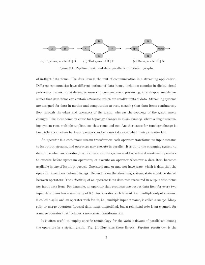
Figure 2.1: Pipeline, task, and data parallelism in stream graphs.

of in-flight data items. The data item is the unit of communication in a streaming application.

Different communities have different notions of data items, including samples in digital signal

processing, tuples in databases, or events in complex event processing; this chapter merely as-

sumes that data items can contain attributes, which are smaller units of data. Streaming systems

are designed for data in motion and computation at rest, meaning that data items continuously

flow through the edges and operators of the graph, whereas the topology of the graph rarely

changes. The most common cause for topology changes is multi-tenancy, where a single stream-

ing system runs multiple applications that come and go. Another cause for topology change is

fault tolerance, where back-up operators and streams take over when their primaries fail.

An operator is a continuous stream transformer: each operator transforms its input streams

to its output streams, and operators may execute in parallel. It is up to the streaming system to

determine when an operator fires; for instance, the system could schedule downstream operators

to execute before upstream operators, or execute an operator whenever a data item becomes

available in one of its input queues. Operators may or may not have state, which is data that the

operator remembers between firings. Depending on the streaming system, state might be shared

between operators. The selectivity of an operator is its data rate measured in output data items

per input data item. For example, an operator that produces one output data item for every two

input data items has a selectivity of 0.5. An operator with fan-out, i.e., multiple output streams,

is called a split, and an operator with fan-in, i.e., multiple input streams, is called a merge. Many

split or merge operators forward data items unmodified, but a relational join is an example for

a merge operator that includes a non-trivial transformation.

It is often useful to employ specific terminology for the various flavors of parallelism among

the operators in a stream graph. Fig. 2.1 illustrates these flavors. Pipeline parallelism is the

9

concurrent execution of a producer A with a consumer B. Task parallelism is the concurrent

execution of different operators D and E that do not constitute a pipeline. And data parallelism

is the concurrent execution of multiple replicas of the same operator G on different portions of the

same data. The architecture community refers to data parallelism as SIMD (single instruction,

multiple data).

2.1 Operator Reordering (a.k.a. hoisting, sinking, rotation, pushdown)

Move more selective operators upstream to filter data early.

BAq0 q1 q2 AB

q0 q1 q2

2.1.1 Example

Consider a healthcare application that continuously monitors patients, alerting physicians when

it detects that a patient requires immediate medical assistance. The input stream contains

patient identification and real-time vital signs. A first operator A enriches each data item with

the full patient name and the result of the last exam by a nurse. The next operator B is a

selection operator, which only forwards data items with alarming vital signs. In this ordering,

many data items will be enriched by operator A and will be sent on stream q1 only to be dropped

by operator B. Hoisting B in front of A eliminates this unnecessary overhead.

2.1.2 Profitability

Reordering is profitable if it moves selective operators before costly operators. The selectivity of

an operator is the number of output data items per input data item. For example, an operator

that drops 70% of all data items outputs only 30% and thus has selectivity 0.3. The chart shows

throughput given two operators A and B of equal cost, where the selectivity of A is fixed at 0.5. If

A comes before B, then independently of the selectivity of B, A processes all data and B processes

50% of the data, so the performance does not change. If B comes before A, then B processes

10

all data, but the amount of data processed by A depends on the selectivity of B, and overall

throughput is higher when B drops more data. The cross-over point is when both are equally

selective.

0.0 0.5 1.0 1.5 2.0

0.00 0.25 0.50 0.75 1.00

Thro

ughp

ut

Selectivity of B

Selection Reordering Not reordered Reordered

2.1.3 Safety

Operator reordering is safe if the following conditions hold:

• Ensure commutativity. The result of executing B before A must be the same as the result

of executing A before B. In other words, A and B must commute. A sufficient condition

for commutativity is if both A and B are stateless. However, there are also cases where

reordering is safe past stateful operators; for instance, in some cases, an aggregation can

be moved before a split.

• Ensure attribute availability. The second operator B must only rely on attributes of the

data item that are already available before the first operator A. In other words, the set of

attributes that B reads from a data item must be disjoint from the set of attributes that A

writes to a data item.

2.1.4 Variations

Algebraic reorderings

Operator reordering is popular in streaming systems built around the relational model, such as

the Stream system [8]. These systems establish the safety of reordering based on the formal

semantics of relational operators, using algebraic equivalences between different operator order-

ings. Such equivalences can be found in standard texts on database systems, such as [41]: besides

11

moving selection operators early to reduce the number of data items, another common optimiza-

tion moves projection operators (operators that strip away some attributes from data items)

early to reduce the size of each data item. And a related optimization picks a relative ordering of

relational join operators to minimize intermediate result sizes: by moving the more selective join

first, the other join has less work. Some streaming systems reorder operators based on extended

algebras that go beyond the relational model. For example, Galax uses nested-relational algebra

for XML processing [95], and Sase uses a custom algebra for finding temporal patterns across

sequences of data items [118]. Finally, commutativity analysis on operator implementations could

be used to discover reorderings even without an operator-level algebra [97]. A practical consid-

eration is whether or not to treat floating point arithmetic as commutative, since floating-point

rounding can lead to different results after reordering.

Synergies with other optimizations

While operator reordering yields benefits of its own, it also interacts with several of the streaming

optimizations cataloged in the rest of this paper. Redundancy elimination (Section 2.2) can be

viewed as a special case of operator reordering, where a Split operator followed by redundant

copies of an operator A is reordered into a single copy of A followed by the Split. Operator

separation (Section 2.3) can be used to separate an operator B into two operators B1 and B2;

this can enable a reordering of one of the operators Bi with a neighboring operator A. After

reordering operators, they can end up near other operators where fusion (Section 2.4) becomes

beneficial; for instance, a selection operator can be fused with a Cartesian-product operator

into a relational join, which is faster because it never needs to create all tuples in the product.

Fission (Section 2.5) introduces parallel segments; when two parallel segments are back-to-back,

reordering the Merge and Split eliminates a serialization bottleneck, as in the Exchange operator

in Volcano [47]. The following figure illustrates this Split/Merge rotation:

Merge Split

Merge

Merge

Split

Split

12

2.1.5 Dynamism

The optimal ordering of operators is often dependent on the input data. Therefore, it is useful

to be able to change the ordering at runtime. The Eddy operator enables a dynamic version

of the operator-reordering optimization with a static graph transformation [12]. As shown in

the figure below, an Eddy operator is connected to every other operator in the pipeline, and

dynamically routes data after measuring which ordering would be the most profitable. This has

the advantage that selectivity need not be known ahead of time, but incurs some extra overhead

for tuple routing.

DCBA

A B

DC

Eddy

2.2 Redundancy Elimination (a.k.a. subgraph sharing, multi-query optimiza-

tion)

Eliminate redundant computations.

DupSplit

A C

A B

C

B

ADupSplit

2.2.1 Example

Consider two telecommunications applications, one of which continuously updates billing infor-

mation, and the other monitors for network problems. Both applications start with an operator

A that deduplicates call-data records and enriches them with caller information. The first ap-

plication consists of operator A followed by an operator B that filters out everything except

long-distance calls, and calculates their costs. The second application consists of operator A

13

followed by an operator C that performs quality control based on dropped calls. Since operator

A is common to both applications, redundancy elimination can share A, thus saving resources.

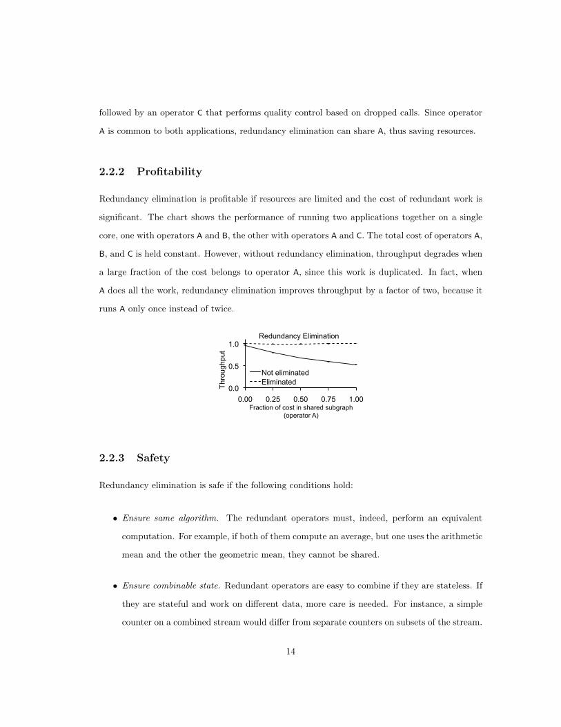
2.2.2 Profitability

Redundancy elimination is profitable if resources are limited and the cost of redundant work is

significant. The chart shows the performance of running two applications together on a single

core, one with operators A and B, the other with operators A and C. The total cost of operators A,

B, and C is held constant. However, without redundancy elimination, throughput degrades when

a large fraction of the cost belongs to operator A, since this work is duplicated. In fact, when

A does all the work, redundancy elimination improves throughput by a factor of two, because it

runs A only once instead of twice.

0.0

0.5

1.0

0.00 0.25 0.50 0.75 1.00

Thro

ughp

ut

Fraction of cost in shared subgraph (operator A)

Redundancy Elimination

Not eliminated Eliminated

2.2.3 Safety

Redundancy elimination is safe if the following conditions hold:

• Ensure same algorithm. The redundant operators must, indeed, perform an equivalent

computation. For example, if both of them compute an average, but one uses the arithmetic

mean and the other the geometric mean, they cannot be shared.

• Ensure combinable state. Redundant operators are easy to combine if they are stateless. If

they are stateful and work on different data, more care is needed. For instance, a simple

counter on a combined stream would differ from separate counters on subsets of the stream.

14

2.2.4 Variations

Multi-tenancy

Redundant subgraphs as described above often occur in streaming systems that are shared by

many different streaming applications. Redundancies are likely when many users launch appli-

cations composed from a small set of data sources and built-in operators. While redundancy

elimination could be viewed as just a special case of operator reordering (Section 2.1), in fact,

the literature has taken it up as a domain in its own right. This separate treatment has been

fruitful, leading to more comprehensive approaches. The Rete algorithm is a seminal technique

for sharing computation between a large number of continuous applications [37]. NiagaraCQ

implements sharing even when operators differ in certain constants, by implementing the op-

erators using relational joins against the table of constants [25]. YFilter implements sharing

between applications written in a subset of XPath, by compiling them all into a combined NFA

(non-deterministic finite automaton) [32].

Other approaches for eliminating operators

Besides the sophisticated techniques for collapsing similar or identical subgraphs, there are other,

more mundane ways to remove an operator from a stream graph. An optimizer can remove a no-

op, i.e., an operator that has no effect, such as a projection that keeps all attributes unmodified;

for example, no-op operators can arise from simple template-based compilers. An optimizer

can remove an idempotent operator, i.e., an operator that repeats the same effect as another

operator next to it, such as two selections in a row based on the same predicate; for example,

idempotent operators can end up next to each other after operator reordering. Finally, an

optimizer can remove a dead subgraph, i.e., a subgraph that never produces any output; for

example, a developer may choose to disable a subgraph for debugging purposes, or a library may

produce multiple outputs, some of which are unused by a particular application.

15

2.2.5 Dynamism

A static compiler can detect and eliminate redundancies, no-ops, idempotent operators, and dead

subgraphs in an application. However, the biggest gains come in the multi-tenancy case, where

the system eliminates redundancies between large numbers of separate applications. In that case,

applications are started and stopped independently. When a new application starts, it should

share any subgraphs belonging to applications that are already running on the system. Likewise,

when an existing application stops, the system should purge any subgraphs that were only used

by this one application. These separate starts and stops necessitate dynamic shared sub-graph

detection, as done for instance in [92]. Some systems take this approach to its extreme, by

treating the addition or removal of applications as a first-class operation just like the addition or

removal of regular data items, e.g., in Rete [37].

2.3 Operator Separation (a.k.a. decoupled software pipelining)

Separate operators into smaller computational steps.

A2A1A

2.3.1 Example

Consider a retail application that continuously watches public discussion forums to discover when

users express negative sentiments about a company’s products. Assume that the input stream

already contains a sentiment score, obtained by a sentiment-extraction operator that analyzes

natural-language text to measure how positive or negative it sounds (not shown). Operator A

filters data items by sentiment and by product. Since operator A has two filter conditions, it can

be separated into two operators A1 and A2. This is an enabling optimization: after separation,

a reordering optimization (Section 2.1) can hoist the product-selection A1 before the sentiment

analysis, thus reducing the number of data items that the sentiment analysis operator needs to

process.

16

2.3.2 Profitability

X Shuffle A X A1 Shuffle A2

Operator separation is profitable if it enables other optimizations such as operator reordering

or fission, or if the pipeline parallelism it creates pays off. We report experiments for operator

reordering and pipeline parallelism elsewhere, in Sections 2.1.2 and 2.4.2, respectively. Therefore,

here, we measure an interaction of operator separation not just with reordering but also with

fission. Consider an application that consists of a first parallel segment X, a Shuffle operator, and

a second parallel segment with an aggregation operator A. Each segment would be replicated 3-

ways, and the shuffle forms a complete bipartite graph. Assume that the cost of the first segment

is negligible, and the cost of the second segment consists of a cost of 0.5 for Shuffle plus a cost of

0.5 for the aggregation A. Therefore, throughput is limited by the second segment. With operator

separation and reordering, the end of the first parallel segment performs a pre-aggregation A1

of cost 0.5 before the Shuffle. At selectivity ≤0.5, at most half of the data reaches the second

segment, and thus, the cost of first segment dominates. Since the cost is 0.5, the throughput is

double of that without optimization. At selectivity 1, all data reaches the second segment, and

thus, the throughput is the same as without operator separation.

0

1

2

3

0.00 0.17 0.33 0.50 0.67 0.83 1.00

Thro

ughp

ut

Selectivity of Aggregation

Separating Aggregation Not separated Separated

2.3.3 Safety

Operator separation is safe if the following condition holds:

• Ensure that the combination of the separated operators is equivalent to the original operator.

Given an input stream s, an operator B can be safely separated into operators B1 and B2

17

only if B2(B1(s)) = B(s). As discussed in Section 2.3.4 below, establishing this equivalence

in the general case is tricky. Fortunately, there are several special cases, particularly in

the relational domain, where it is easier. If B is a selection operator, and the selection

predicate uses logical conjunction, then B1 and B2 can be selections on the conjuncts. If

B is a projection that assigns multiple attributes, then B1 and B2 can be projections that

assign the attributes separately. If B is an idempotent aggregation, then B1 and B2 can

simply be the same as B itself.

2.3.4 Variations

Separability by construction

The safety of separation can be established by algebraic equivalences. Database textbooks list

such equivalences for relational algebra [41], and some streaming systems optimize based on these

algebraic equivalences [8]. Beyond the algebraic approach, MapReduce can separate the Reduce

operator into a preliminary Combine operator and a final Reduce operator if it is associative [29].

This is useful, because subsequently, Combine can be reordered with the shuffle and fused with

the Map operator. Similarly, Yu et al. [122] describe how to automatically separate operators in

DryadLINQ [123] based on a notion of decomposable functions: the programmer can explicitly

provide decomposable aggregation functions (such as Sum or Count), and the compiler can infer

decomposability for certain expressions that call them (such as new T(x.Key, x.Sum(), x.Count())).

Separation by analysis

Separating arbitrary imperative code is a difficult analysis problem. In the compiler community,

this has become known as DSWP (decoupled software pipelining [89]). In contrast to traditional

SWP (software pipelining [67]), which increases instruction-level parallelism in single-threaded

code, DSWP introduces separate threads for the pipeline stages. Ottoni et al. propose a static

compiler analysis for fine-grained DSWP [89]. Thies et al. propose a dynamic analysis for dis-

covering coarse-grained pipelining, which guides users in manually separating operators [111].

18

2.3.5 Dynamism

We are not aware of a dynamic version of this optimization. Separating a single operator into two

requires sophisticated analysis and transformation of the code comprising the operator. However,

the dependent optimizations enabled by operator separation, such as operator reordering, are

often done dynamically, as discussed in the corresponding sections.

2.4 Fusion (a.k.a. superbox scheduling)

Avoid the overhead of data serialization and transport.

BAq0 q1 q2 A

q0 Bq2

2.4.1 Example

Consider a security application that continuously scrutinizes system logs to detect security breaches.

The application contains an operator A that parses the log messages, followed by a selection op-

erator B that uses a simple heuristic to filter out log messages that are irrelevant for the security

breach detection. The selection operator B is light-weight compared to the cost of transferring

a data item from A to B and firing B. Fusing A and B prevents the unnecessary data transfer

and operator firing. The fusion removes the pipeline parallelism between A and B, but since B is

light-weight, the savings outweigh the lost benefits from pipeline parallelism.

2.4.2 Profitability

Fusion trades communication cost against pipeline parallelism. When two operators are fused, the

communication between them is cheaper. But without fusion, they have pipeline parallelism: the

upstream operator can already work on the next data item, while, simultaneously, the downstream

operator is still working on the previous data item. The chart shows throughput given two

operators of equal cost. The cost of the operators is normalized to a communication cost of 1

for sending a data item between non-fused operators. When the operators are not fused, there

19

are two cases: if operator cost is lower than communication cost, throughput is bounded by

communication cost; otherwise, it is determined by operator cost. When the operators are fused,

performance is determined by operator cost alone. The break-even point is when the cost per

operator equals the communication cost, because the fused operator is 2× as expensive as each

individual operator.

0.0 0.5 1.0 1.5 2.0 2.5

0 1 2 3 4 5 6

Thro

ughp

ut

Operator cost / communication cost

Fusion

Not fused Fused

2.4.3 Safety

Fusion is safe if the following conditions hold:

• Ensure resource kinds. The fused operators must only rely on resources, including logical

resources such as local files and physical resources such as GPUs, that are all available on

a single host.

• Ensure resource amounts. The total amount of resources required by the fused operators,

such as disk space, must not exceed the resources of a single host.

• Avoid infinite recursion. If there is a cycle in the stream graph, for example for a feedback-

loop, data may flow around that cycle indefinitely. If the operators are fused and imple-

mented by function calls, this can cause a stack overflow.

2.4.4 Variations

Single-threaded fusion

A few systems use a single thread for all operators, with or without fusion [21]. But in most

systems, fused operators use the same thread, whereas non-fused operators use different threads

20

and can therefore run in parallel. That is the case we refer to as single-threaded fusion. There are

different heuristics for deciding its profitability. StreamIt uses fusion to coarsen the granularity

of the graph to the target number of cores, based on static cost estimates [46]. Aurora uses fusion

to avoid scheduling overhead, picking a fixed schedule that optimizes for throughput, latency, or

memory overhead [23]. Spade and Cola fuse operators as much as possible, but only as long

as the fused operator performs less work per time unit than the capacity of its host, based on

profiling information from a training run [42, 63].

Optimizations enabled by fusion

Fusion often opens up opportunities for traditional compiler optimizations to speed up the code.

For instance, in StreamIt, fusion is followed by constant propagation, scalar replacement, register

allocation, and instruction scheduling across operator boundaries [46]. In relational systems,

fusing two projections into a single projection means that the fused operator needs to allocate

only one data item, not two, per input item. Fusion can also open up opportunities for algorithm

selection (see Section 2.10). For instance, when Sase fuses a source operator that reads input

data with a down-stream operator, it combines them such that the down-stream operator is

piggy-backed incrementally on the source operator, producing fewer intermediate results [118].

Multi-threaded fusion

Instead of combining the fused operators in the same thread of control, fusion may just combine

them in the same address space, but separate threads of control. That yields the benefits of

reduced communication cost, without giving up pipeline parallelism. The fused operators com-

municate data items through a shared buffer. This causes some overhead for locking or copying

data items, except when the operators do not mutate their data items.

2.4.5 Dynamism

Fusion is most commonly done statically. However, the Flextream system performs dynamic

fusion by halting the application, re-compiling the code with the new fusion decisions, and then

resuming the application [57]. This enables Flextream to adapt to changes in available resources,

21

for instance, when the same host is shared with a different application. However, pausing the

application for recompilation causes a latency glitch. Selo et al. mention an even more dynamic

fusion scheme as future work in their paper on transport operators [100]. The idea is to decide

at runtime whether to route a data item to a fused operator in the same process, or to a version

of that same operator in a different process.

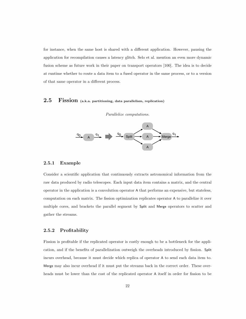
2.5 Fission (a.k.a. partitioning, data parallelism, replication)

Parallelize computations.

Aq0 q1

A

A

A

Split Mergeq0 q1

2.5.1 Example

Consider a scientific application that continuously extracts astronomical information from the

raw data produced by radio telescopes. Each input data item contains a matrix, and the central

operator in the application is a convolution operator A that performs an expensive, but stateless,

computation on each matrix. The fission optimization replicates operator A to parallelize it over

multiple cores, and brackets the parallel segment by Split and Merge operators to scatter and

gather the streams.

2.5.2 Profitability

Fission is profitable if the replicated operator is costly enough to be a bottleneck for the appli-

cation, and if the benefits of parallelization outweigh the overheads introduced by fission. Split

incurs overhead, because it must decide which replica of operator A to send each data item to.

Merge may also incur overhead if it must put the streams back in the correct order. These over-

heads must be lower than the cost of the replicated operator A itself in order for fission to be

22

profitable. The chart shows throughput for fission. Each curve is specified by its p/s/o ratio,

which stands for parallel/sequential/overhead. In other words, p is the cost of A itself, s is the

cost of any sequential part of the graph that is not replicated, and o is the overhead of Split and

Merge. When p/s/o is 1/1/0, the parallel part and the sequential part have the same cost, so no

matter how much fission speeds up the parallel part, the overall time remains the same due to

pipeline parallelism. When p/s/o is 1/0/1, then fission has to overcome an initial overhead equal

to the cost of A, and therefore only turns a profit above two cores. Finally, a p/s/o of 1/0/0

enables fission to turn a profit right away.

0

2

4

6

1 2 3 4 5 6

Thro

ughp

ut

Number of Cores

Fission

p/s/o = 1/1/0 p/s/o = 1/0/1 p/s/o = 1/0/0

2.5.3 Safety

Fission is safe if the following conditions hold:

• If there is state, keep it disjoint, or synchronize it. Stateless operators are trivially safe; they

can be replicated much in the same way that SIMD instructions can operate on multiple

data items at once. Operators with partitioned state can benefit from fission, if the operator

is replicated strictly on partitioning boundaries. An operator with partitioned state is one

that maintains disjoint state based on a particular key attribute of each data item, for

example, a separate average stock price based on the value of the stock-ticker attribute.

Such operators are, in effect, multiple operators already. Applying fission to such operators

makes them separate in actuality as well. Finally, if operators share the same address space

after fission, they can share state as long as they perform proper synchronization to avoid

race conditions.

• If ordering is required, merge in order. Ordering is a subtle constraint, because it is not the

23

operator itself that determines whether ordering matters. Rather, it is the downstream op-

erators that consume the operator’s data items. If an operation is commutative across data

items, then the order in which the data items are processed is irrelevant. If downstream

operators must see data items in a particular order but the operator itself is commutative,

then the transformation must ensure that the output data is combined in the same order

that the input data was partitioned. There are various approaches for re-establishing the

right order, if required. CQL uses logical timestamps [8]. StreamIt uses round-robin or du-

plication [45]. And MapReduce, instead of re-establishing the old order, uses a distributed

“sort” stage [29].

2.5.4 Variations

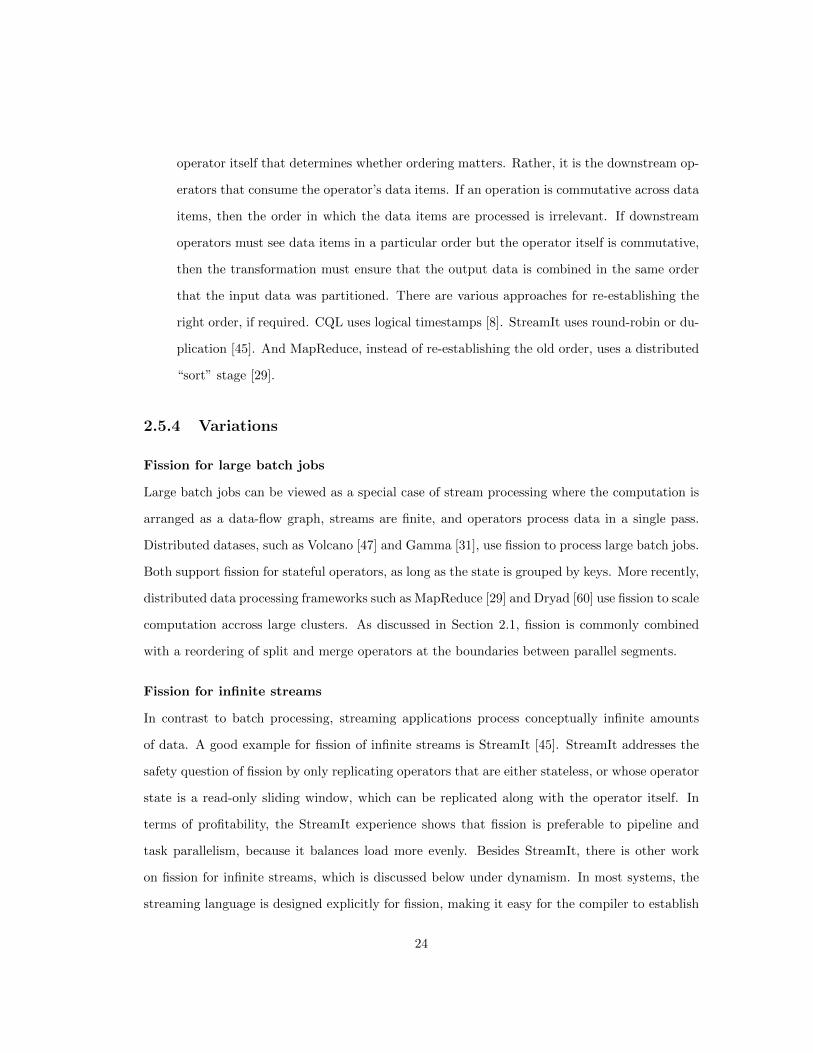
Fission for large batch jobs

Large batch jobs can be viewed as a special case of stream processing where the computation is

arranged as a data-flow graph, streams are finite, and operators process data in a single pass.

Distributed datases, such as Volcano [47] and Gamma [31], use fission to process large batch jobs.

Both support fission for stateful operators, as long as the state is grouped by keys. More recently,

distributed data processing frameworks such as MapReduce [29] and Dryad [60] use fission to scale

computation accross large clusters. As discussed in Section 2.1, fission is commonly combined

with a reordering of split and merge operators at the boundaries between parallel segments.

Fission for infinite streams

In contrast to batch processing, streaming applications process conceptually infinite amounts

of data. A good example for fission of infinite streams is StreamIt [45]. StreamIt addresses the

safety question of fission by only replicating operators that are either stateless, or whose operator

state is a read-only sliding window, which can be replicated along with the operator itself. In

terms of profitability, the StreamIt experience shows that fission is preferable to pipeline and

task parallelism, because it balances load more evenly. Besides StreamIt, there is other work

on fission for infinite streams, which is discussed below under dynamism. In most systems, the

streaming language is designed explicitly for fission, making it easy for the compiler to establish

24

safety. When the language is not designed for fission, safety must be established either by static

or by dynamic dependence analysis. An example for a static analysis that discovers fission

opportunities is parallel-stage decoupled software pipelining [94]. And Thies et al. explore using

dynamic analysis to discover fission opportunities [111].

2.5.5 Dynamism

To make the profitability decision for fission dynamic, we need to dynamically adjust the width of

the parallel segment, in other words, the number of replicated parallel operators. Seda does that

by using a thread-pool controller, which keeps the size of the thread pool below a maximum, but

may adjust to a smaller number of threads to improve locality [114]. MapReduce dynamically

adjusts the number of workers dedicated to the map task [29]. And “elastic operators” adjust

the number of parallel threads based on trial-and-error with observed profitability [99].

To make the safety decision for fission dynamic, we need to dynamically resolve conflicts on

state and ordering. Brito et al. use software transactional memory, where simultaneous updates to

the same state are allowed speculatively, with roll-back if needed [18]. The ordering is guaranteed

by ensuring that transactions are only allowed to commit in the same order in which the input

data arrived.

2.6 Placement (a.k.a. layout)

Assign operators to hosts and cores.

B

D

A

E

C B

D

A

E

C

2.6.1 Example

Consider a telecommunications application that continuously computes usage information for

long-distance calls. The input stream consists of call-data records. The example has three

25

operators: operator A preprocesses incoming data items, operator B selects long-distance calls,

and operator C computes and records billing information for the selected calls. In general, the

stream graph might contain more operators, such as D and E, which perform additional functions,

such as classifying customers based on their calling profile and determining targeted promotions.

If we assume that preprocessing (operator A) and billing (operator C) are both expensive, it

makes sense to place them on different hosts. On the other hand, selection (operator B) is cheap,

but it reduces the data volume substantially. Therefore, it should be placed on the same host

as A, because that reduces the communication cost, by eliminating data that would otherwise

have to be sent between hosts.

2.6.2 Profitability

Placement trades communication cost against resource utilization. When multiple operators are

placed on the same host, they compete for common resources, such as disk, memory, or CPU.

The chart is based on a scenario where two operators compete for disk only. In other words, each

operator accesses a file each time it fires. The two operators access different files, but since there

is only one disk, they compete for the I/O subsystem. The host is a multi-core machine, so the

operators do not compete for CPU. When communication cost is low, the throughput is roughly

twice as high when the operators are on separate hosts because they can each access separate

disks and the cost of communicating across hosts is marginal. When communication costs are

high, the benefit of accessing separate disks is overcome by the expense of communicating across

hosts, and it becomes more profitable to share the same disk even with contention.

0.0 0.5 1.0 1.5 2.0 2.5

0 1 2 3

Thro

ughp

ut

Communication cost

Placement Not colocated Colocated

26

2.6.3 Safety

Placement is safe if the following conditions hold:

• Ensure resource kinds. Placement is safe if each host has the right resources for all the

operators placed on it. For example, source operators in financial stream applications often

run on FPGAs, and the Lime streaming language supports operators on both CPUs and

FPGAs [11]. Operators compiled for an FPGA must be placed on hosts with FPGAs.

• Ensure resource amounts. The total amount of resources required by the fused operators,

such as FPGA capacity, must not exceed the resources of a single host.

• Obey security and licensing restrictions. Besides resource constraints, placement can also be

restricted by security, where certain operators can only run on trusted hosts. In addition to

these technical restrictions, legal issues may also apply. For example, licensing may restrict

a software package to be installed on only a certain number of hosts.

• If placement is dynamic, move only relocatable operators. Dynamic placement requires

operator migration, i.e., moving an operator from one host to another. Doing this safely

requires moving the operator’s state, and ensuring that no in-flight data items are lost in the

switch-over. Depending on the system, this may only be possible for certain operators, for

instance, operators without state, or without OS resources such as sockets or file descriptors.

2.6.4 Variations

Placement for load balancing

Section 2.7 discussed placement algorithms that focus primarily on load balancing [119, 7].

Placement for other constraints

While load balancing is usually at least part of the consideration for placement, often other con-

straints complicate the problem. Pietzuch et al. present a decentralized placement algorithm for

a geographically distributed streaming system, where some operators are geographically pinned

[92]. Soda performs placement for load balancing while also taking into account constraints

27

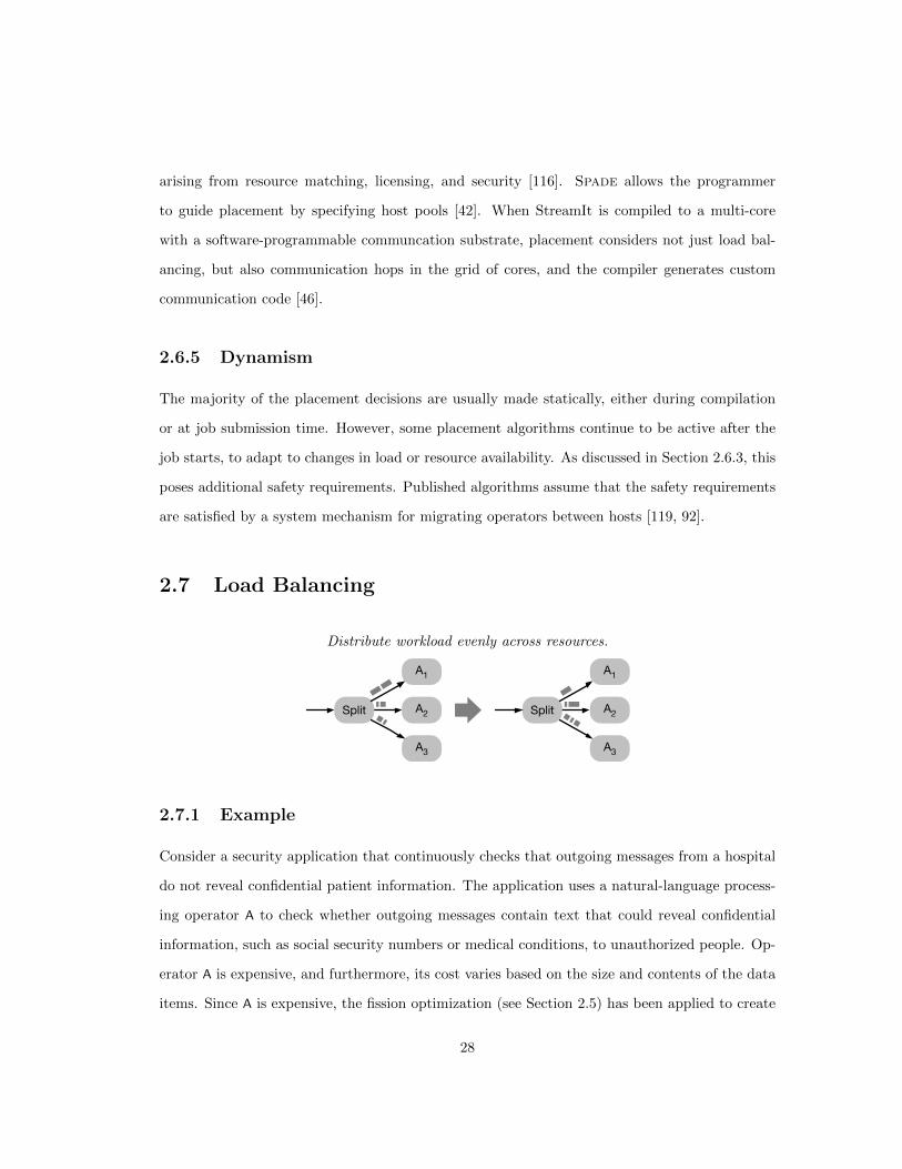
arising from resource matching, licensing, and security [116]. Spade allows the programmer

to guide placement by specifying host pools [42]. When StreamIt is compiled to a multi-core

with a software-programmable communcation substrate, placement considers not just load bal-

ancing, but also communication hops in the grid of cores, and the compiler generates custom

communication code [46].

2.6.5 Dynamism

The majority of the placement decisions are usually made statically, either during compilation

or at job submission time. However, some placement algorithms continue to be active after the

job starts, to adapt to changes in load or resource availability. As discussed in Section 2.6.3, this

poses additional safety requirements. Published algorithms assume that the safety requirements

are satisfied by a system mechanism for migrating operators between hosts [119, 92].

2.7 Load Balancing

Distribute workload evenly across resources.

A1

A2

A3

Split

A1

A2

A3

Split

2.7.1 Example

Consider a security application that continuously checks that outgoing messages from a hospital

do not reveal confidential patient information. The application uses a natural-language process-

ing operator A to check whether outgoing messages contain text that could reveal confidential

information, such as social security numbers or medical conditions, to unauthorized people. Op-

erator A is expensive, and furthermore, its cost varies based on the size and contents of the data

items. Since A is expensive, the fission optimization (see Section 2.5) has been applied to create

28

parallel replicas A1, A2, and A3. When one of the replicas is busy with a message that takes a

long time to process, but another replica is idle, this optimization sends the next message to the

idle replica so it gets processed quickly. In other words, when the load is unevenly distributed,

the optimization balances it to improve overall performance.

2.7.2 Profitability

Load balancing is profitable if it compensates for skew. The chart shows the impact of load

balancing in an experiment consisting of a Split operator that streams data to 3 or 4 replicated

operators. With perfect load balancing, throughput is close to 4 with 4 replicas, and close

to 3 with 3 replicas. Without load balancing, there is skew, and throughput is bounded by

whichever replica receives the most load. For example, with keyed partitions, this replica might

be responsible for data items corresponding to a popular key. If the bottleneck replica receives

33% of the load, then even with a total of 4 replicas, the throughput is only 3.

0.0

1.0

2.0

3.0

4.0

0 20 40 60 80

Thro

ughp

ut

Percent load on bottleneck replica

Load Balancing

Balanced, 4 replicas Balanced, 3 replicas Skewed, 4 replicas

2.7.3 Safety

Load balancing is safe if the following conditions hold:

• Avoid starvation. The work assignment must ensure that every data item eventually gets

processed.

• Ensure each worker is qualified. If load balancing is done after fission, each replica must

be capable of processing each data item. That means replicas must be either stateless or

have access to a common shared state.

29

• Establish placement safety. If load balancing is done while placing operators, the safety

conditions from Section 2.6 must be met.

2.7.4 Variations

Balancing load while placing operators

StreamIt uses fusion (Section 2.4) and fission (Section 2.5) to balance load at compile-time, by

adjusting the granularity of the stream graph to match the target number and capacity of cores

[46]. Xing et al. use operator migration to balance load at runtime, by placing operators on

different hosts if they tend to experience load spikes at the same time, and vice versa [119].

While Xing et al. focus only on computation cost, Wolf et al. use operator placement at job-

submission time to balance both computation cost and communication cost [116]. After placing

operators on hosts, their load can be further balanced via priorities [7].

Balancing load while assigning work to operators

Instead of balancing load by deciding how to arrange the operators, an alternative approach is

to first use fission (Section 2.5) to replicate operators, and then balance load by deciding how

much streaming data each replica gets to process. The distributed queue component in River [10]

offers two approaches for this: in the push-based approach, the producer keeps track of consumer

queue lengths, and uses a randomized credit-based scheme for routing decisions, whereas in the

pull-based approach, consumers request data when they are ready. Another example for the

push-based approach is the use of back-pressure for load balancing in System S [7]. MapReduce

[29] uses the pull-based approach. However, Condie et al. argue that the push-based approach

is more appropriate when adapting MapReduce to streaming [26]. In MapReduce, as in other

systems with fission by keys, the load balance depends on the how evenly the system partitions

the data and the skew in the data. Work stealing is an approach for re-arranging work even after

it has been pushed or pulled to operators [16].

30

2.7.5 Dynamism

As the discussion of variations above shows, there are two main techniques for load balancing:

based on placement, or based on tuple routing. Roughly speaking, the placement-based variants

tend to be static, whereas the routing-based variants are dynamic. Placement has the advantage

that it does not necessarily require fission. Placement can be made dynamic too, but that has

issues: operator migration causes freeze times; if load spikes are sudden, changing the placement

may take too long; and migrating a stateful operator is an engineering challenge [33]. Routing

incurs a frequent small overhead for each data item instead of an occasional large overhead for

each reconfiguration.

2.8 State Sharing (a.k.a. synopsis sharing, double-buffering)

Optimize for space by avoiding unnecessary copies of data.

BA BA

2.8.1 Example

Consider a financial application that continuously computes the volume-weighted average price

and other statistics of stocks for both one hour and one day. Assume that the application

maintains large windows for each aggregation—enough so that their memory requirements may

be substantial fractions of a single host. However, if the only difference between the aggregations

is their time granularity, then they can share the same aggregation window, thereby reducing the

total amount of memory required for both operators.

2.8.2 Profitability

State sharing is profitable if it reduces stalls due to cache misses or disk I/O, by decreasing

the memory footprint. The chart shows the results of an experiment with two operators, both

31

acting on the same stream of data. To provide measurably bad locality, each operator walks a

fixed number of randomly selected locations in the state each time it fires. At low state sizes,

all state fits in the 32KB L1 cache, and throughput for both versions is high. As the state size

increases, the not-shared version does not fit in L1 cache anymore, and its throughput degrades.

Eventually, the shared version does not fit in L1 cache anymore either, but both still fit in L2

cache, so the throughput becomes the same again. This phenomenon is repeated at the L2 cache

size: the throughput of the not-shared version degrades first, and the throughput of the shared

version follows later when it does not fit in L2 cache anymore either.

0.0 0.2 0.4 0.6 0.8 1.0

1 2 4 8 16

32

64

128

256

512

1,02

4

Thro

ughp

ut

State size in KB

State Sharing

Not shared Shared

2.8.3 Safety

State sharing is safe if the following conditions hold:

• Ensure state is visible to both operators. The operators that share the state must have

common access to it. Typically, this is accomplished by fusion, putting them in the same

operating-system process.

• Avoid race conditions. State sharing must prevent race conditions, either by ensuring that

the data is immutable, or by properly synchronizing accesses.

• Manage memory safely. The memory for the shared state is managed properly. It is neither

reclaimed too early, nor is it allowed to grow without bounds, i.e., leak.

2.8.4 Variations

State-sharing techniques vary by what kind of state is being shared. We discuss the prominent

variations from the literature in order from most general to least general.

32

Shared operator state

The most general variant deals with operators that have arbitrary non-trivial state. It imposes

the most challenging requirements on synchronization and memory management. The straight-

forward approach is to use shared memory and mutual-exclusion locks. But when conflicts

are rare, this may unnecessarily restrict concurrency. Therefore, another approach uses STM

(software transactional memory) to manage shared data representing a table or a graph [18].

Shared window

In this variant, multiple consumers can peek into the same window. Even though operators with

windows are technically stateful, this is a simple case of state that is easier to share [45]. CQL

implements windows by non-shared arrays of pointers to shared data items, such that a single

data item might be pointed to from multiple windows and event queues [8].

Shared queue

In this variant, the producer can write a new item into a queue at the same time that the consumer

reads an old item. To ensure proper synchronization without sacrificing actual concurrency or

requiring extra data copies, the queue must have a capacity of at least two data items; therefore,

this variant is sometimes called double-buffering. Sermulins et al. show how to further optimize

a shared queue, by making it local and computing all offsets at compile-time, so that it can be

implemented by scalar variables instead of an array [101]. Once this is done, traditional compiler

optimizations can improve the code even further, by allocating queue entries to registers.

2.8.5 Dynamism

We are not aware of a dynamic version of this optimization: the decision whether or not state can

be shared is made statically. However, once that decision is made, the implementation techniques

can be more or less dynamic. StreamIt uses a fully-static approach, where a static schedule

prescribes exactly what data can be accessed by which operator at a what time [101]. Brito et

al.’s work is more dynamic, where access to shared state is reconciled by software transactional

memory [18].

33

2.9 Batching (a.k.a. train scheduling, execution scaling)

Process multiple data items in a single batch.

A A'

2.9.1 Example

Consider a healthcare application that repeatedly fires an FFT (Fast Fourier Transform) operator

for medical imaging. Efficient FFT implementations contain enough code such that instruction

cache locality becomes an issue. If the FFT is used as an operator in a larger application together

with other operators, batching can amortize the cost of bringing the FFT in cache over multiple

data items. In other words, each time the FFT operator fires, it processes a batch of data items

in a loop. This will increase latency, because data items are held until the batch fills up. But

depending on the application, this latency can be tolerated if it leads to higher fidelity otherwise.

2.9.2 Profitability

Batching trades throughput for latency. Batching can improve throughput by amortizing operator-

firing costs over more data items. Such amortizable costs include calls that might be deeply

nested; warm-up costs, in particular, for the instruction cache; and scheduling costs, possibly in-

volving a context switch. On the other hand, batching leads to worse latency, because a data item

will not be processed as soon as it is available, but only later, when its entire batch is available.

The figure shows this trade-off for batch sizes from 1 to 10 data items. For throughput, higher

is better; initially, there is a large improvement in throughput, but the throughput curve levels

out when the per-batch cost has been amortized. For latency, lower is better; latency increases

linearly with batch size, getting worse the larger the batch is.

34

0

1

2

3

4

1 2 3 4 5 6 7 8 9 10 Batch size

Batching

Throughput Latency

2.9.3 Safety

Batching is safe if the following conditions hold:

• Avoid deadlocks. Batching is only safe if it does not cause deadlocks. Batching can cause

deadlock if the operator graph is cyclic. This happens if an operator waits for a number of

data items to form a batch, but some of those data items must go around a feedback loop,

and the feedback loop is depleted because the operator is waiting. Batching can also cause

deadlock if the batched operator shares a lock with an upstream operator. An example

is if the batched operator waits for a number of data items to form a batch while holding

the lock, thus preventing the upstream operator from sending data items to complete the

batch.

• Satisfy deadlines. Certain applications have hard real-time constraints, others have quality-

of-service (QoS) constraints involving latency. In either case, batching must take care to

keep latency within acceptable levels. For instance, video processing must keep up a frame

rate to avoid jitter.

2.9.4 Variations

Batching is a streaming optimization that plays well into the hands of more traditional (not

necessarily streaming) compiler optimizations. In particular, batching gives rise to loops, and

the compiler may optimize these loops with unrolling or with software pipelining [67]. The

compiler for a streaming language may even combine the techniques directly [101].

35

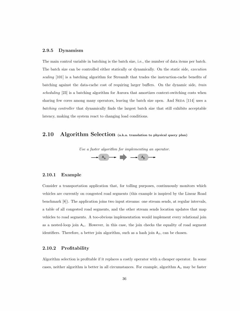
2.9.5 Dynamism

The main control variable in batching is the batch size, i.e., the number of data items per batch.

The batch size can be controlled either statically or dynamically. On the static side, execution

scaling [101] is a batching algorithm for StreamIt that trades the instruction-cache benefits of

batching against the data-cache cost of requiring larger buffers. On the dynamic side, train

scheduling [23] is a batching algorithm for Aurora that amortizes context-switching costs when

sharing few cores among many operators, leaving the batch size open. And Seda [114] uses a

batching controller that dynamically finds the largest batch size that still exhibits acceptable

latency, making the system react to changing load conditions.

2.10 Algorithm Selection (a.k.a. translation to physical query plan)

Use a faster algorithm for implementing an operator.

Aα Aβ

2.10.1 Example

Consider a transportation application that, for tolling purposes, continuously monitors which

vehicles are currently on congested road segments (this example is inspired by the Linear Road

benchmark [8]). The application joins two input streams: one stream sends, at regular intervals,

a table of all congested road segments, and the other stream sends location updates that map

vehicles to road segments. A too-obvious implementation would implement every relational join

as a nested-loop join Aα. However, in this case, the join checks the equality of road segment

identifiers. Therefore, a better join algorithm, such as a hash join Aβ, can be chosen.

2.10.2 Profitability

Algorithm selection is profitable if it replaces a costly operator with a cheaper operator. In some

cases, neither algorithm is better in all circumstances. For example, algorithm Aα may be faster

36

for small inputs and Aβ may be faster for large inputs. In other cases, the algorithms optimize

for different metrics. For example, algorithm Aα may be faster but algorithm Aβ may use less

memory. Finally, there are cases with trade-offs between performance and generality: algorithm

Aα may be faster, but algorithm Aβ may work in a wider set of circumstances. The chart compares

throughput of a nested loop join vs. a hash join. At small window sizes, the performance difference

is in the noise, whereas at large window sizes, the hash join clearly performs better. On the other

hand, hash joins are less general, since their join condition must be an equality, not an arbitrary

predicate.

0.0 0.2 0.4 0.6 0.8 1.0

0 200 400 600 800 1,000

Thro

ughp

ut

Window size

Algorithm Selection

Nested loop join Hash join

2.10.3 Safety

Algorithm selection is safe if the following condition holds:

• Ensure same behavior. Both operators must behave the same for the given inputs. If

algorithm Aα is less general than algorithm Aβ, then choosing the operator with Aα instead

of Aβ is only safe if Aα is general enough for the particular usage. The join example from

Section 2.10.1 illustrates this.

2.10.4 Variations

Physical query plans

The motivating example for this section, where the choice is between a nested-loop join and a

hash join, is common in database systems. Compilers for databases typically first translate an

application (or query) into a graph (or plan) of logical operators, and then translate that to a

graph (or plan) of physical operators [41]. The algorithm selection happens during the transla-

37

tion from logical to physical operators. Join operators in particular have many implementation

choices; for instance, an index lookup join may speed up join conditions like a > 5 with a B-tree.

When join conditions get more complex, deciding the best strategy becomes more difficult. A

related approach is Sase, which can fuse certain operators with the source operator, and then

implement these operators by a different algorithm [118].

Auto-tuners

Outside of streaming systems, there are several successful software packages that perform “em-

pirical optimization”. In order to tune itself to a specific hardware platform, the software pack-

age automatically runs a set of performance experiments during installation to select the best-

performing algorithms and parameters. Prominent examples include Fftw [39], Spiral [120],

and Atlas [115]. Yotov et al. compare this empirical optimization approach to more traditional,

model-based compiler optimizations [121].

Different semantics

Algorithm selection can be used as a simple form of load shedding. While most approaches to

load shedding work by dropping data items (as described in Section 2.11), load shedding by

algorithm selection merely switches to a cheaper implementation. Unlike the other variations of

algorithm selection, this is, by definition, not safe, because the algorithms are not equivalent.

This choice can happen either at job admission time [116], or dynamically, as described below.

2.10.5 Dynamism

When algorithm selection is used to react to runtime conditions, it must be dynamic. In Seda,

each operator can decide its own policy for overload, and one alternative is to provide degraded

service, i.e., algorithm selection [114]. In Borealis, operators have control inputs, for instance,

to select a different algorithm variant for the operator [3]. To implement dynamic algorithm

selection, the compiler statically provisions both variants of the algorithm, and the runtime

system dynamically picks one or the other as needed. In other words, this approach does for

algorithm selection what the Eddy [12] does for operator reordering: it statically inserts a dynamic

38

routing component.

2.11 Load Shedding (a.k.a. admission control, graceful degradation)

Degrade gracefully when overloaded.

A Shedder A

2.11.1 Example

Consider an emergency management application that provides logistics information to police and

fire companies as well as to the general public. Under normal conditions, the system can easily

keep up with the load, and display information to everyone who asks. However, when disaster

strikes, the load can increase by orders of magnitude, and exceed the capacity of the system.

Without load shedding, the requests would pile up, and nobody would get timely responses.

Instead, it is preferable to shed some of the load by only providing complete and accurate replies

to requests from police or fire companies, and degrading accuracy for everyone else.

2.11.2 Profitability

Load shedding improves throughput at the cost of reducing accuracy. Consider an aggregate

operator A that constructs a histogram over windows of 1,000 tuples each, for instance, to visualize

system state in a graphical dash-board. For each window, it counts each data item as belonging

to a “bucket”. The selectivity of an operator is the number of output data items per input

data item. When there is no load shedding, i.e., when selectivity is 1, the histogram has perfect

accuracy, i.e., an accuracy of 1. On the other hand, if the load-shedder only forwards ten out of

every thousand data items, i.e., when selectivity is 0.01, the histogram has a lower accuracy. The

chart measures accuracy as 1 minus error, where the error is the Pythagorean distance between

the actual histogram and the expected histogram.

39

0.0

0.5

1.0

0.00 0.01 0.10 1.00 Selectivity

Load Shedding

Throughput Accuracy

2.11.3 Safety

Unlike the other optimizations in this paper, load shedding is, by definition, not safe. While the

other optimizations try to compute the same result as in the unoptimized case, load shedding

computes a different, approximate, result; the quality of service of the application will degrade.

However, depending on the particular application, this drop in quality may be acceptable. Some

applications deal with inherently imprecise data to begin with: for example, sensor readings from

the physical world have limited precision. Other applications produce outputs where correctness

is not a clear-cut issue: for example, advertisement placement and prioritization. Finally, there

are applications that are inherently resilient to imprecision: for example, iterative page-rank

computation uses a convergence check [90].

2.11.4 Variations

Load shedding in network applications

Network stacks and web servers are vulnerable to load spikes, and load shedding has been a prime

motivator for implementing them as graphs of streams and operators. Receive livelock occurs

when input-processing starves downstream processing to the extent that data items must be

dropped for the system to make progress [81]. The Scout operating system drops data items early

if it can predict that they will miss their deadline [82]. The Click router puts load shedders into

their own separate operators to modularize the application [65]. And in the Seda architecture

for event-based servers, each operator can elect between different approaches for dealing with

overload, by back-pressure, load shedding, or even algorithm selection (see Section 2.10) [114].

40

Load shedding in relational systems

Papers on load shedders for both Aurora and Stream observe that in general, shedders should be

as close to sources as possible, but in the presence of subgraph sharing (see Section 2.2), shedders

may need to be delayed until just after the shared portion [108, 14]. Gedik et al. propose going

one step further, by moving the load shedders out of the streaming system entirely and onto the

sensors that produce the data in the first place [42].

2.11.5 Dynamism

By definition, load shedding is always applied dynamically.

2.12 Discussion

The previous sections surveyed the major streaming optimizations one by one. A bigger pic-

ture emerges when making observations across individual optimizations. This section discusses

these observations, puts them in context, and proposes avenues for future research on streaming

optimizations.

2.12.1 How to specify streaming applications

Not only is there a large number of streaming languages, there are several language families and

other approaches for implementing streaming applications. The programming model is relevant

for optimizations, since it influences how and where they apply. The following list of programming

models is ordered from low-level to high-level. For conciseness, we only list one representative

example for each.

• Non-streaming language. This is the lowest-level approach, where the application is written

in a traditional language like C or Fortran, and the compiler must do all the work of

extracting streams, like in decoupled software pipelining [89].

• Annotated non-streaming language. This approach adds pragmas to indicate streams in a

traditional language like C or Fortran. An example is Brook [19].

41

• Extension to non-streaming language. This approach adds language features to turn a

traditional language like C into a streaming language. An example is Hancock [27].

• Framework in object-oriented language. In this approach, an operator is specified as a

subclass of a class with abstract event-handling methods. Examples are common in the

systems community, e.g., Seda [114].

• Graph, specified textually. Some streaming languages allow the user to specify the stream

graph directly in terms of operators and streams. An example is Spade [42].

• Graph, specified visually. Instead of specifying the stream graph textually in a language,

some systems, such as Aurora, provide a visual environment for that instead [4].

• Graph, composed with combinators. Some streaming languages support graph construc-

tion only with a small set of built-in combinators. For example, StreamIt provides three

combinators: pipeline, split-join, and feedback loop [45].

• Queries written in SQL dialect. The databases community has developed dialects of SQL

for streaming, for example, CQL [8].

• Rules written in Datalog dialect. There are also dialects of logic languages for streaming,

for example, Overlog [74].

• Patterns compiled to automatons. The complex event processing community has developed

pattern languages, which can be compiled into state machines for detecting events on

streams. An example is Sase [118].

• Tag-based planner. This is the highest-level approach, where the user merely selects tags,

and the system synthesizes an application, as in Mario [96]. The user experience more

closely resembles search than programming.

As a rule of thumb, the advantages of low-level approaches are generality (pretty much any

application can be expressed) and predictability (the program will perform as the author expects).

On the other hand, the advantages of high-level approaches are usability (certain applications can

42

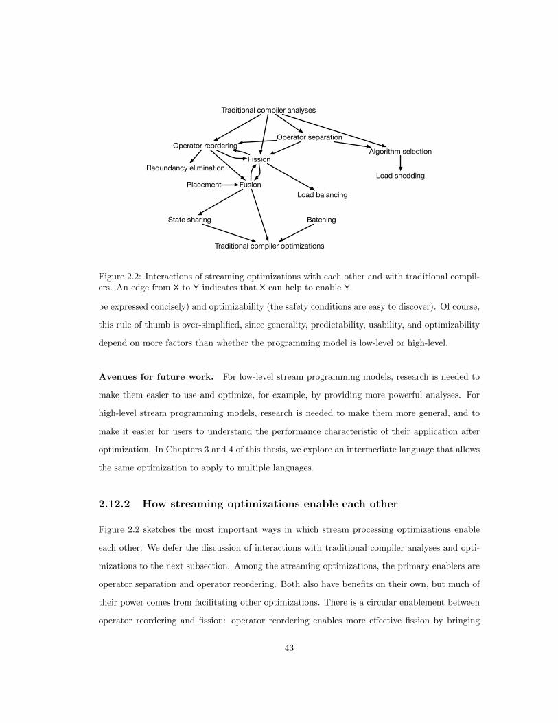
Traditional compiler analyses

Operator separationOperator reordering

Fission

Load balancing

Redundancy elimination

FusionPlacement

BatchingState sharing

Traditional compiler optimizations

Algorithm selection

Load shedding

Figure 2.2: Interactions of streaming optimizations with each other and with traditional compil-ers. An edge from X to Y indicates that X can help to enable Y.

be expressed concisely) and optimizability (the safety conditions are easy to discover). Of course,

this rule of thumb is over-simplified, since generality, predictability, usability, and optimizability

depend on more factors than whether the programming model is low-level or high-level.

Avenues for future work. For low-level stream programming models, research is needed to

make them easier to use and optimize, for example, by providing more powerful analyses. For

high-level stream programming models, research is needed to make them more general, and to

make it easier for users to understand the performance characteristic of their application after

optimization. In Chapters 3 and 4 of this thesis, we explore an intermediate language that allows

the same optimization to apply to multiple languages.

2.12.2 How streaming optimizations enable each other

Figure 2.2 sketches the most important ways in which stream processing optimizations enable

each other. We defer the discussion of interactions with traditional compiler analyses and opti-

mizations to the next subsection. Among the streaming optimizations, the primary enablers are

operator separation and operator reordering. Both also have benefits on their own, but much of

their power comes from facilitating other optimizations. There is a circular enablement between

operator reordering and fission: operator reordering enables more effective fission by bringing

43

operators together that can be part of the same parallel segment, whereas fission enables re-

ordering of the split and merge operators that fission inserts. In addition, fission makes it easier

to balance load, because it introduces data parallelism, which tends to be more homogeneous

and malleable than pipeline or task parallelism. A streaming system that implements multiple

of these optimizations is well advised to apply them in some order consistent with the direction

of the edges in Figure 2.2. It can even make sense to repeatedly attempt optimizations that form

an enabling cycle.

Avenues for future work. Finding the right sequence in which to apply optimizations is an

interesting problem when there are variants of optimizations with complex interactions. Further-

more, while there is literature with cost models for individual optimizations, extending those to

work on multiple optimizations is challenging; in part, that is because the existing cost models

are usually sophisticated and custom-tailored for their optimization.

2.12.3 How streaming optimizations interact with traditional compil-

ers

By traditional compiler, we refer to compilers for languages such as Fortran, C, C++, or Java.

These languages do not have streaming constructs, and rely heavily on functions, loops, arrays,

objects, and similar shared-memory control constructs and data structures. Traditional compilers

excel at optimizing code written in that style.

The top-most part of Figure 2.2 sketches the most important ways in which traditional com-

piler analyses can enable streaming optimizations. Specifically:

• Operator reordering can be enabled by commutativity analysis [97].

• Operator separation can be supported by compiler analysis for decoupled software pipelining

(DSWP) [89].

• Fission can also be supported by compiler analysis for parallel-stage DSWP [89].

• Load balancing can be supported by worst-case execution time (WCET) analysis [71].

44

That does not mean that without compiler analysis, these optimizations are impossible. To

the contrary, many streaming systems apply the optimizations successfully, by using a program-

ming model that is high-level enough to establish certain safety properties by construction.

At the other end, the bottom-most part of Figure 2.2 sketches the most important ways

in which streaming optimizations have been used to enable traditional compiler optimizations.

Specifically:

• Fusion enables function inlining, and that in turn is a core enabler for many other compiler

optimizations, such as constant folding and register allocation.

• State sharing enables scalar replacement, where an array is implemented by one local

variable per array element [101].

• Batching enables loop unrolling and/or software pipelining [67].

In each case, the streaming optimization increases the amount of information available to the

traditional compiler. Note, however, that this in itself does not automatically lead to improved

optimization. Some engineering is usually needed to ensure that the traditional compiler will

indeed take advantage of its optimization opportunities [83]. For instance, when the generated

code uses pointers or deeply-nested calls, the traditional compiler cannot always establish the

safety or profitability of transformations.

Avenues for future work. One fruitful area for research would be new compiler analyses to

help enable streaming optimizations in more general cases. Another area of research is in how to

communicate source-level information to a low-level compiler for optimization of generated code.

2.12.4 Dynamic optimization for streaming systems

Several streaming optimizations have both static and dynamic variants. Table 2.1 summarizes

these variations, and each optimization section has a subsection on dynamism. In general, the

advantages of static optimizations are that they can afford to be more expensive; it is easier to

make them more comprehensive; and it is easier for them to interact with traditional compilers.

45

On the other hand, the advantages of dynamic optimizations are that they are more autonomous;

they have access to more information to support profitability decisions; they can react to changes

in resources or load; and they can even speculate on safety, as long as they have a safe fall-

back mechanism. The literature lists some intermediate approaches, which optimize either at

application launch time, or periodically re-run a static optimizer at runtime, as in Flextream

[57]. This is in contrast to the fully dynamic approach, where the application is transformed for

maximum runtime flexibilities, as in Eddies [12].

Avenues for future work. There are several open problems in supporting more dynamic

optimizations. One is low-overhead profiling and simple cost models to support profitability

trade-offs. Another is the runtime support for dynamic optimization, for instance, efficient and

safe migration of stateful operators.

2.12.5 Assumptions, stated or otherwise

Stream processing has become popular in several independent research communities, and these

communities have different assumptions that influence the shape and feasibility of streaming

optimizations.

Even, predictable, and balanced load. Pretty much all static optimizations make this

assumption. On the other hand, other communities, such as the systems community, assume to

the contrary that load can fluctuate widely. In fact, that is a primary motivation for two of the

optimizations: load balancing and load shedding.

Centralized system. Many optimizations assume shared memory and/or a shared clock, and

are thus not directly applicable to distributed streaming systems. This is true for most cases of

state sharing, and for dynamic techniques such as changing the number of replicas in fission to

adapt to load. Authors of distributed systems tend to emphasize distribution, but it does not

always occur to authors of centralized systems to state the centralized assumptions.

46

Fault tolerance. Many optimizations are orthogonal to whether or not the system is fault

tolerant. However, for some optimizations, making them fault tolerant requires significant addi-

tional effort. An example is the Flux operator, which makes fission fault tolerant by maintaining

hot stand-by operators, and implementing protocols for fault detection, take-over, and catch-up

[102].

Avenues for future work. For any optimization that explicitly states or silently makes re-

strictive assumptions, coming up with a way to overcome the restrictions can be a rewarding

research project. Examples include getting a centralized optimization to work (and scale!) in a

distributed system, or removing the dependence on fault-tolerance from an optimization.

2.12.6 Metrics for streaming optimization profitability

There are many ways to measure whether a streaming optimization was profitable, including

throughput, latency, quality of service (QoS), power, and network utilization. The goals are

frequently in-line with each other: many optimizations that improve throughput will also improve

the other metrics. For that reason, most of this survey focuses on throughput. Notable exceptions

include the trade-off between throughput and latency seen in batching, fission, and operator

separation; the trade-off between throughput and QoS or accuracy in load shedding; and the

trade-off between throughput and power in fission. As a concrete example for such trade-offs,

slack refers to the permissible wiggle-room for degrading latency up to a deadline, which can be

exploited by a controller to optimize throughput [114].

Avenues for future work. For performance evaluation, standard benchmarks would be a

great service to the streaming optimization community. Some examples of existing benchmarking

work are: the BiCEP benchmarks [78], the StreamIt benchmarks [110], and the Stanford stream

query repository which includes the Linear Road [8] application (§ 4.5). However, more work is

needed.

47

2.13 Requirements for a Streaming IL

In addition to the big picture observations, this catalog helps clarify what information a streaming

IL needs to provide in order to support streaming optimizations. Some interesting trends emerge

from the discussion of each operator:

• Four of the eleven optimizations (state sharing, fission, load balancing, and placement)

have output that depends on the order that the operators execute. Fission and placement

are particularly important, since streaming applications must scale across clusters to pro-

cess large data sets. This indicates that an IL for streaming should be explicit in how

deterministic execution is enforced.

• Five of the eleven optimizations (reordering, redundancy elimination, operator separation,

fusion, and fission) modify the topology of the data flow graph. Information about operator

connectivity (i.e. communication) is, therefore, an important requirement for a streaming

IL.

• Eight of the eleven optimizations (redundancy elimination, fission, fusion, separation, re-

ordering, placement, load-balancing, and state sharing) have safety conditions that depend

on the state of an operator. This argues that an IL designed for streaming optimizations

needs information about operator state.

• Nine of the eleven optimizations (operator separation and state sharing being the excep-

tions) have a dynamic variation. This fact argues that a streaming IL should provide

support for dynamism.

• All eleven of the optimizations have at least one unique safety requirement. This suggests

that there is not a finite set of features that an IL can capture to support all optimizations.

Rather, the IL needs to be extensible.

In summary, this catalog of optimizations suggests that an intermediate language for stream

processing should make it explicit how determinism is enforced, and provide information about

48

operator state and connectivity, as that information is required for a many optimizations. It

should also be extensible, so that it can support the unique requirements of each optimization.

Chapters 3 and 4 will show how the intermediate language presented in this thesis meets those

requirements. However, the catalog also argues that a streaming IL should support dynamic

optimizations. Chapter 6 points to this as one of the major limitations in our IL.

2.14 Chapter Summary

This chapter presents a catalog of optimizations for stream processing. It consolidates the ex-

tensive prior optimizations work, and also provides a practical guide for users and implementors.

The challenge in organizing such a catalog is to provide a framework in which to understand the

optimizations. To that end, this chapter is structured in a similar style to catalogs of design pat-

terns or refactoring. This survey establishes a common terminology across the various research

communities that have embraced stream processing. This enables members from the different

communities to easily understand and apply the optimizations, and lays a foundation for contin-

ued research in streaming optimizations. In the overall context of this thesis, this catalog clarifies

what information a streaming IL needs to provide in order to support streaming optimizations.

49

3

The Brooklet Calculus for Stream

Processing

The previous chapter identifies some of the key requirements for a streaming IL that emerge

from the survey of optimizations: no assumption of deterministic execution; explicit state and

communication; extensibility; and support for dynamism. In this chapter, we formalize three of

the requirements—non-determinism, state, and communication—in a calculus. We leave support

for dynamism to future work. Although there are many formal models for streaming systems [9,

62, 68, 70], none of the prior work incorporates these three requirements.

The Brooklet 1 calculus for stream processing [104] defines a core minimal language that was

designed to meet two goals. First, as already mentioned, to enable reasoning about the correctness

of optimizations. Second, it was designed to be flexible enough to represent a diverse set of

streaming languages. Language designers have developed numerous domain-specific streaming

languages [8, 19, 25, 42, 88, 93, 107, 112, 123] that are both tailored to the needs of their particular

applications, and optimized for performance on their particular target runtimes. In this chapter,

we discuss three prominent examples: CQL, StreamIt, and Sawzall:

• CQL [8] and other StreamSQL dialects [107] are popularly used for algorithmic trading.

CQL extends SQL’s well studied relational operators with a notion of windows over infinite

streams of data, and relies on classic query optimizations [8], such as moving a selection

before a join.

• StreamIt [112], a synchronous data-flow language, has been used for MPEG encoding and

decoding [34]. The StreamIt compiler enforces static data transfer rates between user-

defined operators with fixed topologies, and improves performance through operator fusion,

fission, and pipelining [112].

• Sawzall [93], a scripting language for Google’s MapReduce [29] platform, is used for web-

1Brooklet is so named because it is the essence of a stream, and is unrelated to the Brook language [19].

50

related analysis. The MapReduce framework streams data items through multiple copies

of user-defined map operators and then aggregates the results through reduce operators on

a cluster of workstations. We view Sawzall as a streaming language in the broader sense,

and address it in this chapter to showcase the generality of our work.

These three examples by no means comprise an exhaustive list of stream programming languages,

but they are representative of the design space.

The challenge in defining a calculus is deciding what parts of a language constitute the core

concepts that need to be modeled in the formal semantics, and what details can be abstracted

away. The two goals of reasoning optimizations and representing a diverse set of languages guide

our design. First, to understand how a language is implemented, we need to understand how

the operators communicate on a distributed platform. Therefore, Brooklet makes communica-

tion explicit as a core concept. Second, to understand how a language maps to an execution

environment, we need to understand how the state embodied in its operational building blocks

is implemented on a distributed platform. Therefore, Brooklet makes state explicit as a core

concept. Third, to understand how to optimize stream programs, we need to understand how to

enable language-level determinism on top of the inherent implementation-level non-determinism

of a distributed system. Therefore, Brooklet exposes non-determinism as another core concept.

On the other hand, modeling local deterministic computations is well-understood, so our

semantics treat local computations as opaque functions. Since our semantics are small-step, this

abstraction loses none of the fine-grained interleaving effects of the distributed computation.

In this chapter we make the following contributions:

• We define a core calculus for stream processing that is general, and facilitates reasoning

about program implementation by modeling state, communication, and non-determinism

as core concepts.

• We translate CQL, StreamIt, and Sawzall to Brooklet, demonstrating the comprehensive-

ness of our calculus. This translation also defines the first formal semantics for Sawzall.

• We use our calculus to show the conditions that enable three vital optimizations: operator

51

fission, operator fusion, and operator re-ordering.

This sets a foundation for River (§4), which can serve as a common intermediate language for

stream processing with a rigorous formal semantics.

3.1 Notation

Throughout the chapter, an over-bar, as in q, denotes a finite sequence q1, . . . , qn, and the i-th

element in that sequence is written qi, where 1 ≤ i ≤ n. The lower-case letter b is reserved for

lists, and • is an empty list. A comma indicates cons or append, depending on the context; for

example d, b is a list consed from the first item d and the remaining items b. A bag is a set with

duplicates. The notation {e : condition} denotes a bag comprehension: it specifies the bag of

all e’s where the condition is true. The symbol ∅ stands for both an empty set and an empty

bag. If E is a store, then the substitution [v 7→ d]E denotes the store that maps name v to

value d and is otherwise identical to E. Angle brackets identify a tuple. For example, 〈σ, τ〉

is a tuple that contains the elements σ and τ . In inference rules, an expression of the form

d, b = b′ performs pattern matching; it succeeds if the list b′ is non-empty, in which case it binds

d to the first element of b′ and b to the remainder of b′. Pattern-matching also works on other

meta-syntax, such as tuple construction. An underscore character _ indicates a wildcard, and

matches anything. Semantics brackets such as [[Pb ]]pz indicate translation. The subscripts b,c,s,z

stand for Brooklet, CQL, StreamIt, and Sawzall, respectively.

3.2 Brooklet

A stream processing language is a language that hides the mechanics of stream processing;

it notably has built-in support for moving data through computations and for composing the

computations with each other. Brooklet is a core calculus for such stream processing languages.

It is designed to model a diversity of streaming languages, and to facilitate reasoning about

language implementation. To achieve these goals, Brooklet models state, communication, and

non-determinism as core concepts, and abstracts away local deterministic computations.

52

Brooklet syntax:Pb ::= out in op Brooklet programout ::= output q ; Output declarationin ::= input q ; Input declarationop ::= ( q, v ) ← f ( q, v ); Operatorq ::= id Queue identifierv ::= $ id Variable identifierf ::= id Function identifier

Brooklet example: IBM market maker.output result;

input bids, asks;

(ibmBids) ← SelectIBM(bids);

(ibmAsks) ← SelectIBM(asks);

($lastAsk)← Window(ibmAsks);

(ibmSales)← SaleJoin(ibmBids,$lastAsk);

(result,$cnt) ← Count(ibmSales,$cnt);

Brooklet semantics: Fb ` 〈V,Q〉 −→ 〈V ′, Q′〉d, b = Q(qi)

op = (_, _)← f(q, v);

(b′, d′) = Fb(f)(d, i, V (v))

V ′= updateV (op, V, d′)

Q′= updateQ(op, Q, qi, b′)

Fb ` 〈V,Q〉 −→ 〈V ′, Q′〉(E-FireQueue)

op = (_, v)← f(_, _);

updateV (op, V, d) = [v 7→ d]V(E-UpdateV)

op = (q, _)← f(_, _);df , bf = Q(qf )Q′ = [qf 7→ bf ]Q

Q′′ = [∀qi∈q : qi 7→ Q(qi), bi]Q′

updateQ(op,Q, qf , b) = Q′′(E-UpdateQ)

Figure 3.1: Brooklet syntax and semantics.

3.2.1 Brooklet Program Example: IBM Market Maker

As an example of a streaming program, we consider a hypothetical application that trades IBM

stock. Data arrives on two input streams, bids(symbol,price) and asks(symbol,price), and

leaves on the result(cnt,symbol,price) output stream. Since the application is only interested

in trading IBM stock, it filters out all other stock symbols from the input. The application

then matches bid and ask prices from the filtered streams to make trades. To keep the example

simple, we assume that each sale is for exactly one share. The Brooklet program in the bottom

left corner of Fig. 3.1 produces a stream of trades of IBM stock, along with a count of the number

of trades.

3.2.2 Brooklet Syntax

A Brooklet program defines a directed, possibly cyclic, graph of operators containing pure func-

tions connected by FIFO queues. It uses variables to explicitly thread state through operators.

Data items on a queue model network packets in transit. Data items in variables model stored

state; since data items may be lists, a variable may store arbitrary amounts of historical data.

The following line from the market maker application defines an operator:

(ibmSales) ← SaleJoin(ibmBids, $lastAsk);

53

The operator reads data from input queue ibmBids and variable $lastAsk. It passes that data as

parameters to the pure function SaleJoin, and writes the result to the output queue ibmSales.

Brooklet does not define the semantics of SaleJoin. Modeling local deterministic computations

is well-understood [85, 91], so Brooklet abstracts them away by encapsulating them in opaque

functions. On the other hand, a Brooklet program does define explicit uses of state. In the

example, the following line defines a window over the stream ibmAsks:

($lastAsk) ← Window(ibmAsks);

The window contains a single tuple corresponding to the most recent ask for an IBM stock,

and the tuple is stored in the variable $lastAsk. Both the Window and SaleJoin operators access

$lastAsk.

The Window operator writes data to $lastAsk, but does not use the data stored in the variable

in its internal computations. Operators that incrementally update state must both read and

write the same variable, such as in the Count operator:

(result, $cnt) ← Count(ibmSales, $cnt);

Queues that appear only as operator input, such as bids and asks, are program inputs, and

queues that appear only as operator output, such as result, are program outputs. Brooklet’s

syntax uses the keywords input and output to declare a program’s input and output queues. We

say that a queue is defined if it is an operator output or a program input. We say that a queue is

used if it is an operator input or a program output. Variables may be defined and used in several

clauses, since they are intended to thread state through a streaming application. In contrast,

each queue must be defined once and used once. This restriction facilitates using our semantics

for proofs and optimizations. The complete Brooklet grammar appears in Fig. 3.1.

3.2.3 Brooklet Semantics

A program operates on data items from a domain D, where a data item is a general term for

anything that can be stored in queues or variables, including tuples, bags of tuples, lists, or

entire relations from persistent storage. Queue contents are represented by lists of data items.

54

We assume that the transport network is lossless and order-preserving but may have arbitrary

delays, so queues support only push-to-back and pop-from-front operations.

3.2.3.1 Brooklet Execution Configuration.

The function environment Fb maps function names to function implementations. This environ-

ment allows us to treat operator functions as opaque. For example, Fb(SelectIBM) would return

a function that filters out data items whose stock symbol differs from IBM.

At any given time during program execution, the configuration of the Brooklet program is

defined as a pair 〈V,Q〉, where V is a store that maps variable names to data items (in the market

maker example, $cnt is initialized to zero and $lastAsk is initialized to the tuple 〈‘IBM’,∞〉),

and Q is a store that maps queue names to lists of data items (initially, all queues except the

input queues are empty).

3.2.3.2 Brooklet Execution Semantics.

Computation proceeds in small steps. Each step fires Rule E-FireQueue from Fig. 3.1. To

explain this rule, we illustrate each line rule one by one, starting with the following intermediate

configuration of the market maker example:

V =[$lastAsk 7→ 〈‘IBM’, 119〉, $cnt 7→ 0

]

Q =

bids 7→ •, ibmBids 7→

(〈‘IBM’, 119〉, 〈‘IBM’, 124〉

),

asks 7→ •, ibmAsks 7→ •,

ibmSales 7→ •, result 7→ •

d, b = Q(qi) : Non-deterministically select a firing queue qi. For a queue to be eligible as a firing

queue, it must satisfy two conditions: it must be non-empty (because we are binding d, b

to its head and tail), and it must appear as an input to some operator (because we are

executing that operator’s firing function). This step can select any queue satisfying these

two conditions.

E.g., qi = ibmBids, d = 〈‘IBM’, 119〉, b =(〈‘IBM’, 124〉

).

op = (_, _)← f(q, v); : Because of the single-use restriction, qi uniquely identifies an operator.

55

E.g., op = (ibmSales) ← SaleJoin(ibmBids, $lastAsk);.

(b′, d′) = Fb(f)(d, i, V (v)) : Use the function name to look up the corresponding function from

the environment. The function parameters are the data item popped from qi; the index i

relative to the operator’s input list; and the current values of the variables in the operator’s

input list. For each output queue, the function returns a list b′j of data items to append,

and for each output variable, the function returns a single data item d′j to store.

E.g., b′

=((〈‘IBM’, 119, 119〉

)), d′

= •,

d = 〈‘IBM’, 119〉, i = 1, V (v) = 〈‘IBM’,119〉.

V ′ = updateV (op, V, d′) : Update the variables using the output d

′.

E.g., in this example, d′

= •, so V ′ = V .

Q′ = updateQ(op, Q, qi, b′) : Update the queues: remove the popped data item from the firing

queue, and for each output queue, push the corresponding list of output data items. The

example has only one output queue and datum.

E.g., Q′ =

bids 7→ •, ibmBids 7→

(〈‘IBM’, 124〉

),

asks 7→ •, ibmAsks 7→ •,

ibmSales 7→(〈‘IBM’, 119, 119〉

), result 7→ •

3.2.4 Brooklet Execution Function

We denote a program’s input 〈V,Q〉 as Ib and an output 〈V ′, Q′〉 as Ob. Given a function

environment Fb, program Pb, and input Ib, the function →∗b (Fb, Pb, Ib) yields the set of all final

outputs. An execution yields a final output when no queue is eligible to fire. Due to non-

determinism, the set may have more than one element. One possible output Ob of our running

example is:

V =[$lastAsk 7→ 〈‘IBM’, 119〉, $cnt 7→ 1

]Q =

bids 7→ •, asks 7→ •, ibmSales 7→ •,

ibmBids 7→ •, ibmAsks 7→ •, result 7→(〈1, ‘IBM’, 119〉

)

The example illustrates the finite case. However, in general, streams are conceptually infinite.

To use our semantics in the general case, we use a theoretical result from prior work: if a stream

56

program is computable, then one can generalize from all finite prefixes of an infinite stream to

the infinite case [50]. If →∗b yields the same result for all finite inputs to two programs, then we

consider these two programs equivalent even on infinite inputs.

3.2.5 Brooklet Summary

Brooklet is a core calculus for stream processing. We designed it to model a diverse set of

streaming languages, and to facilitate reasoning about program implementation. Brooklet mod-

els communication through explicit queues, thus making it clear where an implementation needs

to send data. It models state through explicit variables, thus making it clear where an implemen-

tation needs to store data. Finally, Brooklet captures inherent non-determinism by not specifying

which queue to fire for each step, thus permitting all interleavings possible in a distributed im-

plementation.

3.3 Language Mappings

We demonstrate Brooklet’s generality by mapping three streaming languages CQL, StreamIt, and

Sawzall to it. Each translation exposes communication as explicit queues; exposes implicit uses

of state as explicit variables; exposes a mechanism for implementing global determinism on top

of an inherently non-deterministic runtime; and abstracts away local deterministic computations

with higher-order wrappers that statically bind the original function and dynamically adapt the

runtime arguments (thus preserving small step semantics).

3.3.1 CQL and Stream-Relational Algebra

CQL, the Continuous Query Language, is a member of the StreamSQL family of languages.

StreamSQL gives developers who are familiar with SQL’s select-from-where syntax an incre-

mental learning path to stream programming. This chapter uses CQL to represent the entire

StreamSQL family, because it has a clean design, has made significant impact [8], and has a

formal semantics [9].

57

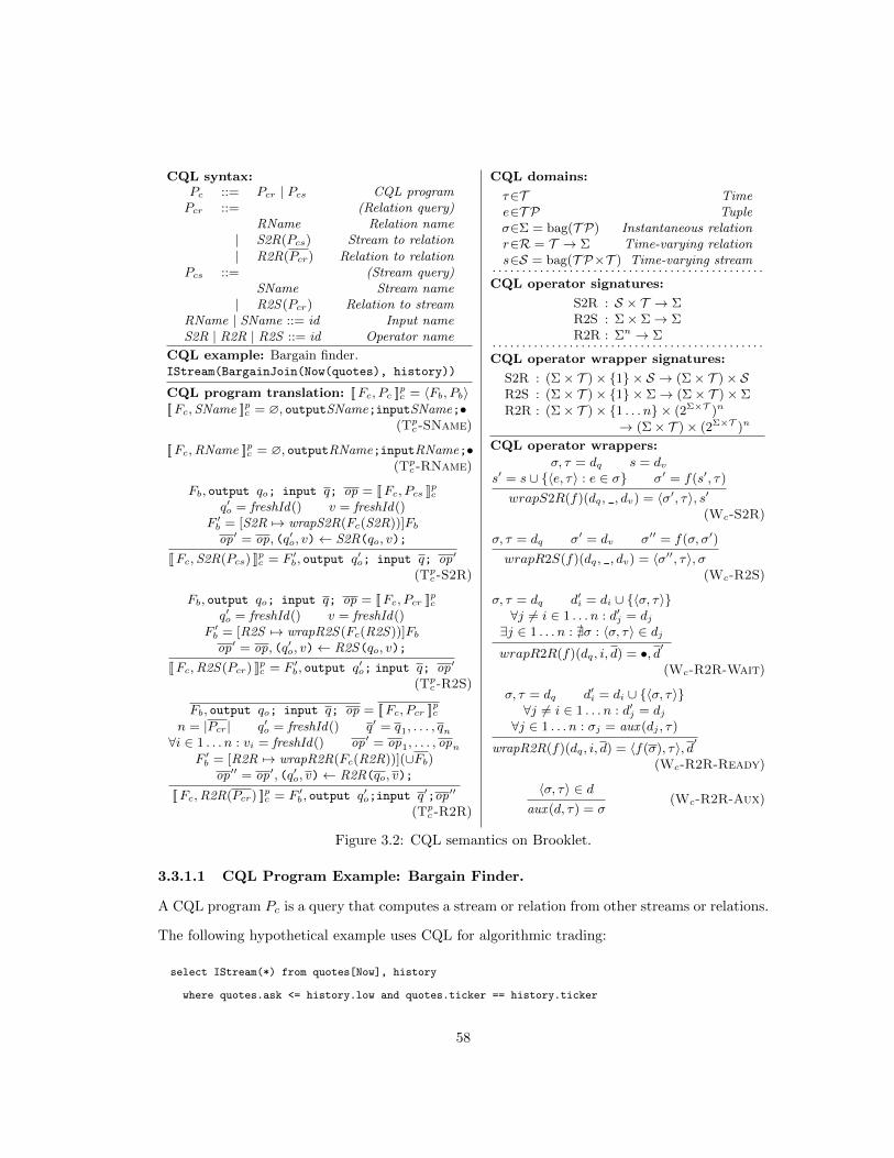
CQL syntax:Pc ::= Pcr | Pcs CQL programPcr ::= (Relation query)

RName Relation name| S2R(Pcs) Stream to relation

| R2R(Pcr) Relation to relationPcs ::= (Stream query)

SName Stream name| R2S(Pcr) Relation to stream

RName | SName ::= id Input nameS2R | R2R | R2S ::= id Operator name

CQL example: Bargain finder.IStream(BargainJoin(Now(quotes), history))

CQL program translation: [[Fc, Pc ]]pc = 〈Fb, Pb〉[[Fc,SName ]]pc = ∅, outputSName;inputSName;•

(Tpc-SName)

[[Fc,RName ]]pc = ∅, outputRName;inputRName;•(Tpc-RName)

Fb, output qo; input q; op = [[Fc, Pcs ]]pcq′o = freshId() v = freshId()

F ′b = [S2R 7→ wrapS2R(Fc(S2R))]Fbop′ = op, (q′o, v)← S2R(qo, v);

[[Fc,S2R(Pcs) ]]pc = F ′b, output q′o; input q; op′

(Tpc-S2R)

Fb, output qo; input q; op = [[Fc, Pcr ]]pcq′o = freshId() v = freshId()

F ′b = [R2S 7→ wrapR2S(Fc(R2S))]Fbop′ = op, (q′o, v)← R2S(qo, v);

[[Fc,R2S(Pcr) ]]pc = F ′b, output q′o; input q; op′

(Tpc-R2S)

Fb, output qo; input q; op = [[Fc, Pcr ]]pcn = |Pcr| q′o = freshId() q′ = q1, . . . , qn∀i ∈ 1 . . . n : vi = freshId() op′ = op1, . . . , opn

F ′b = [R2R 7→ wrapR2R(Fc(R2R))](∪Fb)op′′ = op′, (q′o, v)← R2R(qo, v);

[[Fc,R2R(Pcr) ]]pc = F ′b, output q′o;input q′;op′′

(Tpc-R2R)

CQL domains:

τ∈T Timee∈T P Tupleσ∈Σ = bag(T P) Instantaneous relationr∈R = T → Σ Time-varying relations∈S = bag(T P×T ) Time-varying stream

. . . . . . . . . . . . . . . . . . . . . . . . . . . . . . . . . . . . . . . . . . . . . .CQL operator signatures:

S2R : S × T → ΣR2S : Σ× Σ→ ΣR2R : Σn → Σ

. . . . . . . . . . . . . . . . . . . . . . . . . . . . . . . . . . . . . . . . . . . . . .CQL operator wrapper signatures:

S2R : (Σ× T )× {1} × S → (Σ× T )× SR2S : (Σ× T )× {1} × Σ→ (Σ× T )× ΣR2R : (Σ× T )× {1 . . . n} × (2Σ×T )n

→ (Σ× T )× (2Σ×T )n

CQL operator wrappers:

σ, τ = dq s = dvs′ = s ∪ {〈e, τ〉 : e ∈ σ} σ′ = f(s′, τ)

wrapS2R(f)(dq, _, dv) = 〈σ′, τ〉, s′(Wc-S2R)

σ, τ = dq σ′ = dv σ′′ = f(σ, σ′)

wrapR2S(f)(dq, _, dv) = 〈σ′′, τ〉, σ(Wc-R2S)

σ, τ = dq d′i = di ∪ {〈σ, τ〉}∀j 6= i ∈ 1 . . . n : d′j = dj∃j ∈ 1 . . . n : @σ : 〈σ, τ〉 ∈ djwrapR2R(f)(dq, i, d) = •, d′

(Wc-R2R-Wait)

σ, τ = dq d′i = di ∪ {〈σ, τ〉}∀j 6= i ∈ 1 . . . n : d′j = dj∀j ∈ 1 . . . n : σj = aux (dj , τ)

wrapR2R(f)(dq, i, d) = 〈f(σ), τ〉, d′

(Wc-R2R-Ready)

〈σ, τ〉 ∈ daux (d, τ) = σ

(Wc-R2R-Aux)

Figure 3.2: CQL semantics on Brooklet.

3.3.1.1 CQL Program Example: Bargain Finder.

A CQL program Pc is a query that computes a stream or relation from other streams or relations.

The following hypothetical example uses CQL for algorithmic trading:

select IStream(*) from quotes[Now], history

where quotes.ask <= history.low and quotes.ticker == history.ticker

58

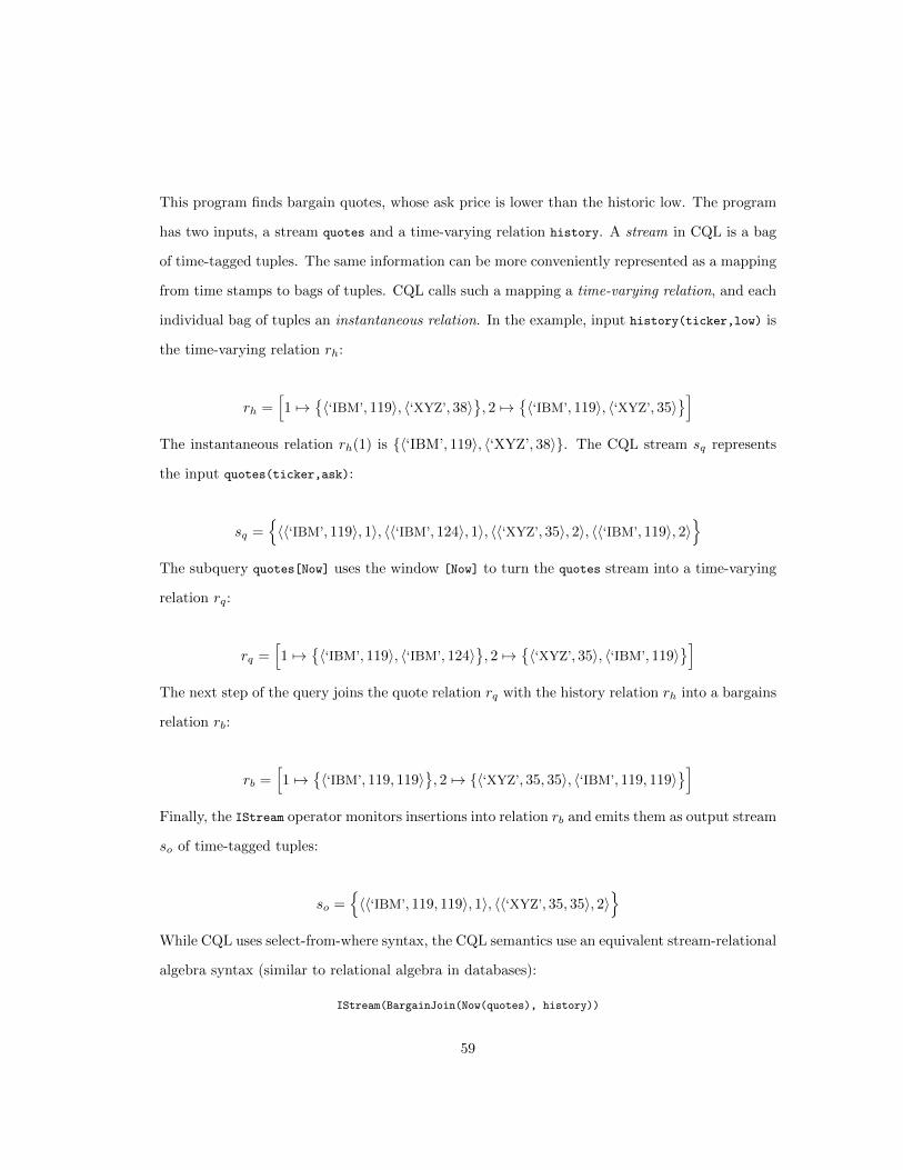
This program finds bargain quotes, whose ask price is lower than the historic low. The program

has two inputs, a stream quotes and a time-varying relation history. A stream in CQL is a bag

of time-tagged tuples. The same information can be more conveniently represented as a mapping

from time stamps to bags of tuples. CQL calls such a mapping a time-varying relation, and each

individual bag of tuples an instantaneous relation. In the example, input history(ticker,low) is

the time-varying relation rh:

rh =[1 7→

{〈‘IBM’, 119〉, 〈‘XYZ’, 38〉

}, 2 7→

{〈‘IBM’, 119〉, 〈‘XYZ’, 35〉

}]The instantaneous relation rh(1) is {〈‘IBM’, 119〉, 〈‘XYZ’, 38〉}. The CQL stream sq represents

the input quotes(ticker,ask):

sq ={〈〈‘IBM’, 119〉, 1〉, 〈〈‘IBM’, 124〉, 1〉, 〈〈‘XYZ’, 35〉, 2〉, 〈〈‘IBM’, 119〉, 2〉

}The subquery quotes[Now] uses the window [Now] to turn the quotes stream into a time-varying

relation rq:

rq =[1 7→

{〈‘IBM’, 119〉, 〈‘IBM’, 124〉

}, 2 7→

{〈‘XYZ’, 35〉, 〈‘IBM’, 119〉

}]The next step of the query joins the quote relation rq with the history relation rh into a bargains

relation rb:

rb =[1 7→

{〈‘IBM’, 119, 119〉

}, 2 7→ {〈‘XYZ’, 35, 35〉, 〈‘IBM’, 119, 119〉

}]Finally, the IStream operator monitors insertions into relation rb and emits them as output stream

so of time-tagged tuples:

so ={〈〈‘IBM’, 119, 119〉, 1〉, 〈〈‘XYZ’, 35, 35〉, 2〉

}While CQL uses select-from-where syntax, the CQL semantics use an equivalent stream-relational

algebra syntax (similar to relational algebra in databases):

IStream(BargainJoin(Now(quotes), history))

59

This algebraic notation makes the operator tree clearer. The leaves are stream name quotes and

relation name history. CQL has three categories of operators. S2R operators turn a stream into

a relation; e.g., Now(quotes) turns stream quotes into relation rq. R2R operators turn one or

more relations into a new relation; e.g., BargainJoin(rq, rh) turns relations rq and rh into the

bargain relation rb. Finally, R2S operators turn a relation into a stream; e.g., IStream(rb) turns

relation rb into the stream of its insertions. CQL has no S2S operators, because they would be

redundant. CQL’s R2R operators coincide with traditional database relational algebra.

The CQL grammar is in Fig. 3.2. A CQL program Pc can be either a relation query Pcr or a

stream query Pcs, and queries are either simple identifiers RName or SName, or composed using

operators from the categories S2R, R2R, or R2S.

3.3.1.2 CQL Implementation Issues.

Before we translate CQL to Brooklet, let us discuss the three issues of communication, state,

and non-determinism in CQL.

CQL communication. In CQL, communication between operators is implicit. The commu-

nication becomes explicit by translating a CQL query into its relational algebra equivalent.

CQL state. CQL represents global state explicitly as named relations, such as the history

relation from our running example. But in addition, all three kinds of CQL operators implicitly

maintain local state, referred to as “synopses” in [8]. An S2R operator maintains the state of

a window on a stream to produce a relation. An R2S operator stores the previous state of the

relation to compute the stream of differences. Finally, an R2R operator uses state to buffer data

from whichever relation is available first, so it can be retrieved later to compute an output when

data with matching time stamps is available for all relations.

CQL non-determinism. CQL is deterministic in the sense that the output of a program is

fully determined by the times and values of its inputs [9]. CQL requires that data arrive in order.

That is, an operator never receives a data item with a lower time stamp than previously received

60

item. Time stamps may be assigned to inputs in two ways. First, a CQL implementation might

assign time stamps to data using its own system time. In this case, there is no difficulty in

satisfying the ordering requirement. Second, an application might include time stamps as part of

its data, such as quotes arriving from a stock exchange. Time stamps from an application may

have ambiguities, such as result from unsynchronized application clocks or non-order preserving

data transmissions. In this case, a CQL implementation must resolve the ambiguities and ensure

the proper ordering of data before it is input to the streaming system [105]. However, a CQL

implementation does not fully determine the order in which operators execute. Thus, a CQL

implementations can permit non-determinism to exploit parallelism. For example, in the query

BargainJoin(Now(quotes), history), the operators Now and BargainJoin can run in parallel in

separate processes, as long as BargainJoin always waits for its two inputs to have the same time

stamp.

Translation to Brooklet will make all communication and state explicit, and will clarify how

the implementation enforces determinism.

3.3.1.3 CQL Translation Example.

Given the CQL example program from Fig. 3.2, the translation to Brooklet is the program Pb:

output qo;

input quotes, history;

(qq, $vn) ← wrapNow(quotes, $vn);

(qb, $vq, $vh) ← wrapBargainJoin(qq, history, $vq, $vh);

(qo, $vo) ← wrapIStream(qb, $vo)

The leaves of the query tree serve as input queues; each subquery produces an intermediate

queue, which the enclosing operator consumes; and the outermost query operator produces the

program output queue. The translation to Brooklet makes the state of the operators explicit. The

most interesting state is that of the wrapBargainJoin operator. Like each R2R operator, it has a

function Fc(BargainJoin) that transforms one or more input instantaneous relations of the same

time stamp to one output instantaneous relation. Brooklet models the choice of interleavings by

allowing either queue qq or history to fire independently. Hence, the Brooklet operator processes

61

one data item each time either queue fires. Assume a data item arrives on the first queue qq.

If there is already a data item with the same time stamp in the variable vh associated with the

second queue, Brooklet performs the join, which may yield data items for the output queue qb.

Otherwise, it simply stores the data item in vq for later.

3.3.1.4 CQL Translation.

Fig. 3.2 shows the translation from CQL to Brooklet by recursion over the input program. Besides

building up a program, the translation also builds up a function environment, which it populates

with wrappers for the original functions. The translation introduces state, which the Brooklet

wrappers maintain and consult to hand the right input to the wrapped CQL functions. Working

in concert, the rules enforce a global convention: the execution sends exactly one instantaneous

relation on every queue at every time stamp. Operators retain historical data in variables, e.g.,

to implement windows.

3.3.1.5 CQL Discussion.

CQL is an SQL dialect for streaming [8]. Arasu and Widom specify big-step denotational se-

mantics for CQL [9]. We show how to translate CQL to Brooklet, thus giving an alternative

semantics. As we will show below, both semantics define equivalent input/output behavior for

CQL programs. Translations from other languages can use similar techniques, i.e., make state ex-

plicit as variables; wrap computation in small-step firing functions; and define a global convention

for how to achieve determinism.

3.3.2 StreamIt and Synchronous Data Flow

StreamIt [113, 112] is a streaming language tailored for parallel implementations of applications

such as MPEG decoding [34]. At its core, StreamIt is a synchronous data flow (SDF) lan-

guage [70], which means that each time an operator fires, it consumes a fixed number of data

items and produces a fixed number of data items. In the MPEG example, data items are pictures.

StreamIt distinguishes between primitive and composite operators. A primitive operator (filter

in StreamIt terminology) has optional local state. A composite operator is either a pipeline, a

62

split-join, or a feedback loop. A pipeline puts operators in sequence, a split-join puts them in

parallel, and a feedback loop puts them in a cycle. The topology of a StreamIt program is re-

stricted to well-nested compositions of these. All StreamIt operators and programs have exactly

one input and one output. We only focus on StreamIt’s SDF core here, and encapsulate the

local deterministic part of the computation in opaque pure functions, while keeping the parts

of the computation that are relevant to streaming. We omit non-core features such as teleport

messaging [34], which delivers control messages between operators and which could be modeled

in Brooklet through shared variables.

3.3.2.1 StreamIt Program Example: MPEG Decoder.

The following example StreamIt program Ps is based on a similar example by Drake et al. [34].

pipeline {

splitjoin {

split roundrobin;

filter { work { tf ← FrequencyDecode(peek(1)); push(tf); pop(); }}

filter { work { tm ← MotionVecDecode(peek(1)); push(tm); pop(); }}

join roundrobin;

}

filter { s; work { s,tc ← MotionComp(s,peek(1)); push(tc); pop(); }}

}

It illustrates how the StreamIt language can be used to decode MPEG video. The example uses

a pipeline and a split-join to compose three filters. Each filter has a work function, which peeks

and pops from its predecessor stream, computes a temporary value, and pushes to its successor

stream. In addition, the MotionComp filter also has an explicit state variable s for storing a

reference picture between iterations. The full syntax of Streamit is in Appendix B.

3.3.2.2 StreamIt Implementation Issues.

As before, we first discuss the intuition for the implementation before giving the details of the

translation.

63

StreamIt communication. Communication between primitive operators in StreamIt is deter-

mined by how they are placed in composite operators. All operators are arranged hierarchally in

either a pipeline, a split-join, or a feedback loop. Translation to Brooklet flattens the hierarchy.

StreamIt state. Filters can have explicit state, such as s in the example. Furthermore, since

Brooklet queues support only push and pop but not peek, the translation of StreamIt will have

to buffer data items in a state variable until enough are available to satisfy the maximum peek()

argument in the work function. Round-robin splitters also need a state variable with a cursor

that determines where to send the next data item. A cursor is simply an index relative to the

splitter. It keeps track of which queue is next in round-robin order. Round-robin joiners also

need a cursor, plus a buffer for any data items that arrive out of turn.

StreamIt non-determinism. StreamIt, at the language level, is deterministic. Furthermore,

since it is an SDF language, the number of data items peeked, popped, and pushed by each oper-

ator is constant. At the same time, StreamIt permits pipeline-, task-, and data-parallelism. This

gives an implementation different scheduling choices, which Brooklet models by non-deterministically

selecting a firing queue. Despite these non-deterministic choices, an implementation must en-

sure deterministic end-to-end behavior, which our translation makes explicit with buffering and

synchronization.

3.3.2.3 StreamIt Translation Example.

StreamIt program translation turns the StreamIt MPEG decoder Ps from earlier into a Brooklet

program Pb:

output qout;

input qin;

(qf, qm, $sc) ← wrapRRSplit-2(qin, $sc);

(qfd, $f) ← wrapFilter-FrequencyDecode(qf, $f);

(qmd, $m) ← wrapFilter-MotionVecDecode(qm, $m);

(qd, $fd, $md, $jc) ← wrapRRJoin-2(qfd, qmd, $fd, $md, $jc);

(qout, $s, $mc) ← wrapFilter-MotionComp(qd, $s, $mc);

64

Each StreamIt filter becomes a Brooklet operator. StreamIt composite operators are reflected

in Brooklet’s operator topology. StreamIt’s SplitJoin yields separate Brooklet split and join

operators. The stateful filter MotionComp has two variables: $s models its explicit state s, and

$mc models its implicit buffer.

3.3.2.4 StreamIt Translation.

StreamIt program xlation excerpt:

f = freshId()v = freshId()

Fb = [f 7→ wrapRRSplit(|q|)]op = (q, v)← f(qa, v);

[[Fs, split roundrobin;, q, qa ]]ps = Fb, op(Tps-RR-Split)

f= freshId()∀i ∈ 0 . . . |q′| : vi = freshId()Fb = [f 7→ wrapRRJoin(|q′|)]

op = (qz, v)← f(q′, v);

[[Fs, join roundrobin;, qz, q′ ]]ps = Fb, op

(Tps-RR-Join)

StreamIt operator wrappers excerpt:

c′ = c+ 1 mod N bv = din∀i ∈ 1 . . . N, i 6= c : bi = •

wrapRRSplit(N)(din, _, c) = b, c′(Ws-RR-Split)

d′i = din, di ∀j 6= i ∈ 1 . . . N : d′j = djd′′c , dout = d′c ∀j 6= c ∈ 1 . . . N : d′′j = d′j

bout , c′, d′′′

= wrapRRJoin(N)(•, i, c+ 1 mod N, d′′)

wrapRRJoin(N)(din , i, c, d) = (bout , dout), c′, d′′′

(Ws-RR-Join-Ready)

∀j 6= i ∈ 1 . . . N : d′j = dj d′i = din, di dc = •wrapRRJoin(N)(din , i, c, d) = •, c, d′

(Ws-RR-Join-Wait)

Figure 3.3: StreamIt round-robin split and join semantics on Brooklet.

We give only a high-level overview of the StreamIt translation here (the details are in Ap-

pendix B). Similarly to CQL, there are recursive translation rules, one for each language con-

struct. The base case is the translation of filters, and the recursive cases compose larger topologies

for pipelines, split-joins, and feedback loops. Feedback loops turn into cyclic Brooklet topologies.

The most interesting aspect are the helper rules for split and join, because they use explicit

Brooklet state to achieve StreamIt determinism. Fig. 3.3 shows the rules. The input to the

splitter is a queue qa, and the output is a list of queues q; conversely, the input to the joiner is a

list of queues q′, and the output is a single queue qz. Both the splitter and the joiner maintain a

cursor to keep track of the next queue in round-robin order. The joiner also stores one variable

for each queue, to buffer data that arrives out-of-turn.

3.3.2.5 StreamIt Discussion.

Our translation from StreamIt to Brooklet yields a program with maximum scheduling flexibility,

allowing any interleavings as long as the end-to-end behavior matches the language semantics.

65

This makes it amenable to distributed implementation. In contrast, StreamIt compilers [112]

statically fix one schedule, which also determines where intermediate results are buffered. The

buffering is implicit state, and StreamIt also has explicit state in filters. As we will see in

Section 3.4, state affects the applicability of optimizations. Prior work on formal semantics for

StreamIt does not model state [113]. By modeling state, our Brooklet translation facilitates

reasoning about optimizations.

3.3.3 Sawzall and MapReduce

Sawzall syntax:

Pz ::= out in emit Sawzall programout ::= t : table f; Output aggregatorin ::= q : input; Input declarationemit ::= emit t[f(q)] ← f(q); Emit statementq ::= id Queue namef ::= id Function namet ::= id Table name

Sawzall example: Query log analyzer.queryOrigins : table sum;

queryTargets : table sum;

logRecord : input;

emit queryOrigins[getOrigin(logRecord)]←1;

emit queryTargets[getTarget(logRecord)]←1;

Sawzall program xlation: [[Fz, Pz, R ]]pz=〈Fb, Pb〉

out , qin: input;, emit = Pz∀i ∈ 1 . . . R : qi = freshId()∀i ∈ 1 . . . R : vi = freshId()fMap = wrapMap(Fz, emit , R)fReduce = wrapReduce(Fz, out)

Fb = [Map 7→ fMap, Reduce 7→ fReduce]opm = (q)← Map(qin);

∀i ∈ 1 . . . R : opi = (vi)← Reduce(qi,vi);op′ = opm, op

[[Fz, Pz, R ]]pz = Fb, output • ;input qin;op′(Tpz)

Sawzall domains:k1 ∈K1 Input key k2 ∈K2 Output keyx1 ∈X1 Input value x2 ∈X2 Output valuet ∈T Aggregate name Oz ∈K2→X2 Output table

Sawzall operator signatures:

fk : K1 ×X1 → K2 fx : K1 ×X1 → X ∗2fa : X2 ×X2 → X2

Sawzall operator wrapper signa-tures:

Map : (K1 ×X1)× {1} → (T × K2 ×X2)∗

Reduce: (T × K2 ×X2)× {1} ×Oz → Oz

Sawzall operator wrappers:

emit t[fk(_)]← fx(_); = emit

b = wrapMap(Fz, emit , R)(d, 1)k1, x1 = d k2 = Fz(fk)(k1, x1)

x2 = Fz(fx)(k1, x1) i = hash(k2) mod Rb′i = bi, 〈t, k2, x21〉, . . . , 〈t, k2, x2n〉∀j 6= i ∈ 1 . . . R : b′j = bj

wrapMap(Fz, (emit , emit), R)(d, _) = b′

(Wz-Map)

∀i ∈ 1 . . . R : bi = •wrapMap(Fz, •, R)(_, _) = b

(Wz-Map-•)

t, k2, x2 = dq t : table fa[]; ∈ outk2 ∈ dv x′2 = Fz(fa)(x2, dv(k2))

d′v = [k2 7→ x′2]dv

wrapReduce(Fz, out)(dq, _, dv) = d′v(Wz-Reduce)

t, k2, x2 = dq t : table fa[]; ∈ outk2 6∈ dv d′v = [k2 7→ x2]dv

wrapReduce(Fz, out)(dq, _, dv) = d′v(Wz-Reduce-∅)

Figure 3.4: Sawzall semantics on Brooklet.

Sawzall [93] is a scripting language for MapReduce [29], which exploits cluster of workstations

to analyze a massive but finite sequence of key/value pairs streamed from disk. In Sawzall, a

66

stateless map operator transforms data one key/value pair at a time, feeding into a stateful reduce

operator. The reduce operator works on separate keys separately, incrementally aggregating

all values for a key into a single value. Although Sawzall programs are batch jobs, they use

incremental operators to process large quantities of data in a single pass, and we therefore

consider it a streaming language. Our translation provides the first formal semantics for Sawzall.

In MapReduce, computation proceeds in four stages. First, each map operator writes its

output to its own local disk as a set of key/value pairs. Second, a shuffle stage copies all the data

for a particular key from all the mappers to the local disk of the reducer responsible for that key.

Third, a sort stage sorts the data for that key. Lastly, the reducer aggregates the sorted data.

Our translation of Sawzall produces a version of the MapReduce paradigm that is more

consistent with a streaming model, and is closer to MapReduce online [26] than to traditional

MapReduce. There is no shuffle stage. Instead, the mapper sends data directly to the appropriate

reducer. There is no sort stage. Data is processed as it arrives, not in sorted order. Consequently,

the reduce function must be associative and commutative. Finally, the reducer outputs results

incrementally, rather than producing a single result based on the entire data set. We assume

that the number of reducers is set ahead of time to a number R, which is consistent with the

description in Pike et al.’s paper [93]. A streaming model allows for increased pipelining and

resource utilization.

3.3.3.1 Sawzall Program Example: Query Log Analyzer.

The example Sawzall program in Fig. 3.4 is based on a similar example in [93]. The program

analyzes a query log to count queries per latitude and longitude, which can then be plotted on

a world map. This program specifies one invocation of the map operator, and uses table clauses

to specify sum as the reduce operator. The map operator transforms its input logRecord into two

key/value pairs:

〈k, x〉 = 〈getOrigin(logRecord), 1〉

〈k′, x′〉= 〈getTarget(logRecord), 1〉

Here, getOrigin and getTarget are pure functions that compute the latitude and longitude of the

host issuing the query and the host serving the result, respectively. The latitude and longitude

67

together serve as the key into the tables. Since the number 1 serves as the value associated with

the key, the sum aggregators end up counting query log entries by key. Fig. 3.4 shows the Sawzall

grammar.

3.3.3.2 Sawzall Implementation Issues.

All Sawzall programs have the same topology, and have stateful and non-deterministic imple-

mentations.

Sawzall communication. The Sawzall translation is simpler than that of CQL or StreamIt,

because each translated program uses the same simple topology. The implementation in Pike

et al.’s paper [93] partitions the reducer key space into R parts, where R is a command-line

argument upon job submission. There are multiple instances of the reduce operator, one per

partition. Thus, the translation hard-codes the data parallelism for the reducers, but generates

only one mapper, deferring data parallelism for mappers to a separate optimization step. Our

translation does not have a shuffle step. Rather, the mapper sends data to the appropriate

reducer directly.

Sawzall state. The map operator is stateless, whereas the reduce operator is stateful, using

state to incrementalize its aggregation. Because reduction works independently per key, each

instance of the reduce operator can maintain the state for its assigned part of the key space

independently.

Sawzall non-determinism. At the language level, Sawzall is deterministic. Sawzall is de-

signed for MapReduce, and the strength of MapReduce is that at the implementation level, it

runs on a cluster of workstations for scalability. To exploit the parallelism of the cluster, at the

implementation level, MapReduce makes non-deterministic dynamic scheduling decisions. Re-

ducers can start while map is still in process, and different reducers can work in parallel with

each other. Different mappers can also work in parallel; we will use Brooklet to address this

optimization later in the chapter, and describe a translation with a single map operator for now.

68

3.3.3.3 Sawzall Translation Example.

Given the Sawzall program Pz from earlier, assuming R = 4 partitions, the Brooklet version Pb

is:

output; /*no output queue, outputs are in variables*/

input qlog;

(q1, q2, q3, q4) ← Map(qlog); /*getOrigin/getTarget*/

($v1) ← Reduce(q1, $v1);

($v2) ← Reduce(q2, $v2);

($v3) ← Reduce(q3, $v3);

($v4) ← Reduce(q4, $v4);

There is one reduce operator for each of the R partitions. Each reducer performs the work for

both aggregators (queryOrigins and queryTargets) from the original Sawzall program. The final

reduction results are in variables $v1. . .$v4.

3.3.3.4 Sawzall Translation.

Fig. 3.4 specifies the program translation, domains, and operator wrappers. There is only one

program translation rule Tpz. The translation [[Fz, Pz, R ]]pz takes the Sawzall function environ-

ment, the Sawzall program, and the number of reducer partitions as arguments. All the emit

statements become part of the single map operator. The map operator wrapper uses a hash

function to scatter its output over the reducer key space for load balancing. All the out declara-

tions become part of each of the reduce operators. Each reducer’s variable stores the mapping

from each key in that reducer’s partition to the latest reduction result for that key. If the key is

new, rule Wz-Reduce-∅ fires and registers x2 as the initial value. At the end of the run, the

results in the variables are deterministic, because aggregators are associative and reducers work

on disjoint parts of the key space.

3.3.3.5 Sawzall Discussion.

There was no prior formal semantics for Sawzall, but Lammel studies MapReduce and Sawzall

by implementing an emulation in Haskell [68]. Now that we have seen how to translate three lan-

guages, it is clear that it is possible to model additional streaming languages or language features

69

on Brooklet. For example, Brooklet can serve as a basis for modeling teleport messaging [34] by

using shared variables for out-of-stream communication between operators.

3.3.4 Translation Correctness

We formulate correctness theorems for CQL and StreamIt with respect to their formal seman-

tics [9, 113]. The proofs are in Appendix A and C. We do not formulate a theorem for Sawzall,

because it lacks formal semantics; our mapping to Brooklet provides the first formal semantics

for Sawzall.

Theorem 3.1 (CQL translation correctness). For all CQL function environments Fc, programs

Pc, and inputs Ic, the results under CQL semantics are the same as the results under Brooklet

semantics after translation [[Fc, Pc ]]pc .

Theorem 3.2 (StreamIt translation correctness). For all StreamIt function environments Fs,

programs Ps, and inputs Is, the results under StreamIt semantics are the same as the results

under Brooklet semantics after translation [[Fs, Ps ]]ps.

3.4 Optimizations

The previous section used our calculus to understand how a language maps to an execution

platform. This section uses our calculus to specify how to use three vital optimizations: operator

fission, operator fusion, and operator re-ordering. Each optimization comes with a correctness

theorem. The proofs are in the Appendix. The correctness of the optimizations dependes on

reasoning about state and communication, requirements identified in by the optimizations catalog

in Section 2.13.

3.4.1 Operator Fission

If an operation is commutative across data items, then the order in which the data items are

processed is irrelevant. MapReduce uses this observation to exploit the collective computing

power of a cluster for analyzing extremely large data sets [29]. The input data set is partitioned,

70

and copies of the map operator process the partitions in parallel. In general, the challenge in

exploiting such data parallelism is determining if an operator commutes. Sawzall and StreamIt

solve this challenge by restricting the programming model. In Brooklet, commutativity analysis

can be performed with a simple code inspection. Since a pure function always commutes2, and

all state in Brooklet is explicit in an operator’s signature, a sufficient condition for introducing

fission is that an operator does not access variables. The transformation must ensure that the

output data is combined in the same order that the input data was partitioned. Brooklet can use

the round-robin splitter and joiner described in the StreamIt translation for this purpose. Thus,

the operator (out)←wrapMap-LatLong(q); can be parallelized with N = 3 copies like this:

(q1, q2, q3, $sc) ← Split(q, $sc);

(q4) ← wrapMap-LatLong(q1);

(q5) ← wrapMap-LatLong(q2);

(q6) ← wrapMap-LatLong(q3);

(out, $v4, $v5, $v6, $jc) ← Join(q4, q5, q6, $v4, $v5, $v6, $jc);

The following rule describes how to create the new program with N duplicates of the parallelized

operator.

op = (qout)← f(qin);

∀i ∈ 1 . . . n : qi = freshId() ∀i ∈ 1 . . . n : q′i = freshId()

F ′b, ops = [[∅, split roundrobin, q, qin ]]ps

∀i ∈ 1 . . . n : opi = (q′i)← f(qi);

F ′′b , opj = [[∅, join roundrobin, qout , q′ ]]ps

〈Fb, op〉 −→Nsplit 〈Fb ∪ F ′b ∪ F ′′b , ops op opj〉

(Ob-Split)

The precondition is that op does not refer to any state variables. The fission optimization

illustrates that Brooklet facilitates reasoning over shared state. The rules for round-robin split

and join are in Fig. 3.3.

Making multiplexers explicit and fixing the degree of parallelism are important to faithfully

model and reason about real-world systems. Possible implementation strategies for avoiding the

limitation of a fixed degree of parallelism include using just-in-time compilation to do splitting

2At least in the mathematical sense; in systems, floating point operations do not always commute.

71

online, or putting code on a larger number of machines and then in practice using only a subset

as needed.

Theorem 3.3 (Correctness of Ob-Split). For all function environments Fb, Brooklet programs

Pb, and degrees of parallelism N , if rule Ob-Split yields 〈Fb, Pb〉 −→Nsplit 〈F ′b, P ′b〉, then

→∗b (Fb, Pb, Ib) =→∗b (F ′b, P′b, Ib) for all Brooklet inputs Ib.

The proof sketch is in Appendix D.

3.4.2 Operator Fusion

In practice, transmitting data between two operators can incur significant overhead. Data needs

to be marshalled/unmarshalled, transferred over a network or written to a mutually accessible

location, and buffered by the receiver, not to mention the expense of context switching. This

overhead can be offset by fusing two operators into one. StreamIt applies this optimization to

operators in a pipelined topology [112]. Operators may be fused if they meet two conditions.

First, they appear in a simple pipeline. Brooklet makes this topology easy to validate because

queues are defined and used exactly once. Second, the state used by the operators must not be

modifiable anywhere else in the program. Again, because Brooklet requires an explicit declaration

of all state, this condition can be verified with a simple code inspection. The following Brooklet

program shows two steps in an MPEG decoder:

(q1,$v1) ← ZigZag(qin,$v1);

(qout,$v2) ← IQuantization(q1,$v2);

The fused equivalent of the program is:

(qout,$v1,$v2) ← Fused-ZigZag-IQuant(qin,$v1,$v2);

The following rule formalizes this optimization:

op1 = (q1, v1)←f1(qin, v1); (∃op′ = (_, v1)←f ′(_, _))⇒ op′ = op1

op2 = (qout , v2)←f2(q1, v2); (∃op′ = (_, v2)←f ′(_, _))⇒ op′ = op2

f = freshId() F ′b = [f 7→ fusedOperator(Fb, f1, f2)]Fb

Fb, op1 op2 −→ F ′b, (qout , v1, v2)← f(qin , v1, v2);

(Ob-Fuse)

72

The preconditions guard against other operators writing variables v1 or v2. The following rule

defines the new internal function:

(dtemp , d′1) = Fb(f1)(din , 1, d1) (dout , d

′2) = Fb(f2)(dtemp , 1, d2)

fusedOperator(Fb, f1, f2)(din , _, d1, d2) = (dout , d′1, d′2)

(Wb-Fuse)

In our example, this combines Fb(ZigZag) and Fb(IQuantization) into function

F ′b(Fused-ZigZag-IQuant). The fusion optimization illustrates that Brooklet facilitates reasoning

over topologies.

Theorem 3.4 (Correctness of Ob-Fuse). For all function environments Fb and Brooklet pro-

grams Pb, if rule Ob-Fuse yields 〈Fb, Pb〉 −→Fuse 〈F ′b, P ′b〉, then →∗b (Fb, Pb, Ib) =→∗b (F ′b, P′b, Ib)

for all Brooklet inputs Ib.

The proof sketch is in Appendix E.

3.4.3 Reordering of Operators

A general rule of thumb for database query optimizations is that it is better to remove more

tuples early in order to reduce downstream computations. The most popular example for this is

hoisting a select operator, because a select reduces the tuple volume for operators it feeds into [8].

A select is said to commute with another operator if their output result is the same regardless of

their execution order. The following program computes the commission on sales of IBM stock.

The input is sale(ticker, price) and the output is commission(ticker, cost). The commission

is 2%.

output commission;

input sale;

(qt) ← BrokerCommission(sale);

(commission) ← Select-IBM(qt);

The functions for the two operators are:

Fb(BrokerCommission)(d, _)= let 〈ticker, price〉 = d in 〈ticker, 0.02 · price〉

Fb(Select-IBM)(d, _)= let 〈ticker, cost〉 = d in if ticker=‘IBM’ then d else •

73

We can reorder the two operators for two reasons. First, the BrokerCommission operator is

stateless, and therefore operates on each data item independently, so its semantics do not change

when it sees a filtered stream of data item. Second, the Select-IBM operator only reads the

ticker, and BrokerCommission forwards the ticker unmodified. In other words, Select-IBM does

not rely on any data modified by BrokerCommission and vice versa. The optimized program is:

output commission;

input sale;

(qt) ← Select-IBM(sale);

(commission) ← BrokerCommission(qt);

The following rule encodes the optimization:

op1 = (qt)← f1(q); op2 = (qout)← f2(qt);

Fb(f1)(d, i) = let 〈r, w〉 = d in 〈r, f1(w, i)〉

Fb(f2)(d, _) = let 〈r, _〉 = d in if f2(r) then d else •

∀i ∈ 1 . . . |q| : q′i = freshId()

op′1 = (qout)← f1(q′); ∀i ∈ 1 . . . |q| : opi = (q′i)← f2(qi);

Fb, op1 op2 −→ Fb, op op′1

(Ob-HoistSelect)

The first two preconditions restrict op1 and op2 to be stateless operators. The third precondition

specifies that f1 forwards a part r of the data item unmodified, and the fourth precondition

specifies that f2 is a select that only reads r, and forwards the entire data item unmodified. We

have chosen in Brooklet to abstract away local deterministic computations into opaque functions,

because their semantics are well-studied (e.g., [36, 43, 97]). We leverage this prior work by

assuming that a static program analysis can determine the restrictions on the read and write sets

of operator functions used for select hoisting.

Theorem 3.5 (Correctness of Ob-HoistSelect). For all function environments Fb and Brooklet

programs Pb, if 〈Fb, Pb〉 −→HoistSelect 〈F ′b, P ′b〉 by rule Ob-HoistSelect, then

→∗b (Fb, Pb, Ib) =→∗b (F ′b, P′b, Ib) for all Brooklet inputs Ib.

The proof sketch is in Appendix F.

74

3.4.4 Optimizations Summary

We have used our calculus to understand how a language can apply three vital optimizations. The

concise and straightforward formalization of the optimizations validates the design of Brooklet.

As shown in Table 2.1, there are many other streaming optimizations. Furthermore, there are

stronger variants of the optimizations we sketched; for example, it is sometimes possible to

introduce data parallelism even for stateful operators. We believe that the examples in this

section are a useful first step towards formalizing optimizations for stream processing languages.

3.5 Chapter Summary

This chapter presents Brooklet, a core calculus for stream processing. It represents stream

processing applications as a graph of operators. Operators contain pure functions, communicate

through explicit queues, thread all state through explicit variables, and trigger non-deterministically.

Explicit state, communication, and non-deterministic execution are central concepts, capturing

the reality of distributed implementations. We translate three representative languages, CQL,

Sawzall, and StreamIt, to Brooklet, thus demonstrating its generality for language designers. We

formalize three vital optimizations, operator fission, operator fusion, and operator reordering, in

Brooklet, thus demonstrating its usefulness for language implementors. As we discuss in Chap-

ter 4, Brooklet provides the foundation for River, a common intermediate language for stream

processing.

75

4

From a Calculus to an Intermediate

Language for Stream Processing

It is widely accepted that intermediate languages help programming languages by decoupling

them from the target platform and vice versa. At its core, an intermediate language provides

a small interface with well-defined behavior, facilitating robust, portable, and economic lan-

guage implementations. Similarly, a calculus is a formal system that mathematically defines

the behavior of the essential features of a domain. This chapter demonstrates how to use a

calculus as the foundation for an intermediate language for stream processing. Stream process-

ing makes it easy to exploit parallelism on multicores or even clusters. Streaming languages

are diverse [8, 11, 42, 93, 112], because they address many real-world domains, including trans-

portation, audio and video processing, network monitoring, telecommunications, healthcare, and

finance.

The starting point for this chapter is the Brooklet calculus. A Brooklet application is a

stream graph, where each edge is a conceptually infinite stream of data items, and each vertex

is an operator. Each time a data item arrives on an input stream of an operator, it fires,

executing a pure function to compute data items for its output streams. Optionally, an operator

may also maintain state, consisting of variables to remember across operator firings. Chapter 3

demonstrated that Brooklet is general enough to model three different streaming languages.

The finishing point for this chapter is the River intermediate language. Extending a calculus

into an intermediate language is challenging. A calculus deliberately abstracts away features

that are not relevant in theory, whereas an intermediate language must add them back in to be

practical. The question is how to do that while (1) maintaining the desirable properties of the

calculus, (2) making the source language development effort economic, and (3) safely supporting

common optimizations and reaching reasonable target-platform performance. The answers to

these questions are the research contributions of this chapter.

On the implementation side, we wrote front-ends for dialects of three very different streaming

76

languages (CQL [8], Sawzall [93], and StreamIt [112]) on River. We wrote a back-end for River

on System S [6], a high-performance distributed streaming runtime. And we wrote three high-

level optimizations (placement, fusion, and fission) that work at the River level, decoupled from

and thus reusable across front-ends. This is a significant advance over prior work, where source

languages, optimizations, and target platforms are tightly coupled. For instance, since River’s

target platform, System S, runs on a cluster of commodity machines, this chapter reports the

first distributed CQL implementation, making CQL more scalable.

Overall, this chapter shows how to get the best of both theory and practice for stream

processing. Starting from a calculus supports formal proofs showing that front-ends realize

the semantics of their source languages, and that optimizations are safe. And finishing in an

intermediate language lowers the barrier to entry for new streaming language implementations,

and thus grows the ecosystem of this crucial style of programming.

4.1 Maintaining Properties of the Calculus

Being a calculus, Brooklet makes abstractions. In other words, it removes irrelevant details

to reduce stream processing to the features that are essential for formal reasoning. On the

other hand, River, being a practical intermediate language, has to take a stand on each of the

abstracted-away details. This section describes these decisions, and explains how the intermediate

language retains the benefits of the calculus.

4.1.1 Brooklet Abstractions and their Rationale

The following is a list of simplifications in the Brooklet semantics, along with the insights behind

them.

Atomic steps. Brooklet defines execution as a sequence of atomic steps. Being a small-step

operational semantics makes it amenable to proofs. Each atomic step contains an entire operator

firing. By not sub-dividing firings further, it avoids interleavings that unduly complicate the

behavior. In particular, Brooklet does not require complex memory models.

77

Pure functions. Functions in Brooklet are pure, without side effects and with repeatable

results. This is possible because state is explicit and separate from operators. Keeping state

separate also makes it possible to see right away which operators in an application are stateless

or stateful, use local or shared state, and read or write state.

Opaque functions. Brooklet elides the definition of the functions for operator firings, because

semantics for local sequential computation are well-understood.

Non-determinism. Each step in a Brooklet execution non-deterministically picks a queue

to fire. This non-deterministic choice abstracts away from concrete schedules. In fact, it even

avoids the need for any centralized scheduler, thus enabling a distributed system without costly

coordination. As discussed in Section 3.3, source languages can implement determinism on top of

Brooklet by adding the appropriate protocols. For example, CQL uses time stamps and StreamIt

uses static data transfer rates with order-preserving joiners and splitters.

No physical platform. Brooklet programs are completely independent from any actual ma-

chines they would run on.

Finite execution. Stream processing applications run conceptually forever, but a Brooklet

execution is a finite sequence of steps. One can reason about an infinite execution by induction

over each finite prefix [50].

4.1.2 River Concretizations and their Rationale

This section shows how the River intermediate language fills in the holes left by the Brooklet

calculus. For each of the abstractions from the previous section, it briefly explains how to

concretize it and why. The details and correctness arguments for these points come in later

sections.

Atomic steps. Whereas Brooklet executes firings one at a time, albeit in non-deterministic

order, River executes them concurrently whenever it can guarantee that the end result is the

78

same. This concurrency is crucial for performance. To guarantee the same end result, River uses

a minimum of synchronization that keeps firings conceptually atomic. River shields application

developers from the concerns of locking or memory models.

Pure functions. Both the calculus and the execution environment separate state from op-

erators. However, whereas the calculus passes variables in and out of functions by copies, the

intermediate language uses pointers instead to avoid the copying cost. Using the fact that state is

explicit, River automates the appropriate locking discipline where necessary, thus relieving users

from this burden. Furthermore, instead of returning data items to be pushed on output queues,

functions in River directly invoke call-backs for the run-time library, thus avoiding copies and

simplifying the function implementations.

Opaque functions. Functions for River are implemented in a traditional non-streaming lan-

guage. They are separated from the River runtime library by a well-defined API. Since atom-

icity is preserved at the granularity of operator firings, River does not interfere with any local

instruction-reordering optimizations the low-level compiler or the hardware may want to perform.

Non-determinism. Being an intermediate language, River ultimately leaves the concrete sched-

ule to the underlying platform. However, it reduces the flexibility for the scheduler by bounding

queue sizes, and by using back-pressure to prevent deadlocks when queues fill up.

No physical platform. River programs are target-platform independent. However, at deploy-

ment time, the optimizer takes target-platform characteristics into consideration for placement.

Finite execution. River applications run indefinitely and produce timely outputs along the

way, fitting the purpose and intent of practical stream processing applications.

In the following sections, we discuss in more detail how River provides a practical realization

of the Brooklet calculus. In particular, we discuss how River maximizes the concurrent execution

of operators while preserving the sequential semantics of Brooklet (§ 4.1.3); uses back-pressure to

79

avoid buffer overflows in the presence of bounded queues(§ 4.1.4); and provides an implementation

language for operator implementation(§ 4.2).

4.1.3 Maximizing Concurrency while Upholding Atomicity

This section gives the details for how River upholds the sequential semantics of Brooklet. In

particular, River differs from Brooklet in how it handles state variables and data items pushed

on output queues. These differences are motivated by performance goals: they avoid unnecessary

copies and increase concurrency.

River requires that each operator instance is single-threaded and that all queue operations are

atomic. Additionally, if variables are shared between operator instances, each operator instance

uses locks to enforce mutual exclusion. River’s locking discipline follows established practice for

deadlock prevention, i.e., an operator instance first acquires all necessary locks in a standard

order, then performs the actual work, and finally releases the locks in reverse order. Otherwise,

River does not impose further ordering constraints. In particular, unless prevented by locks,

operator instances may execute in parallel. They may also enqueue data items as they execute

and update variables in place without differing in any observable way from River’s call-by-value-

result semantics. To explain how River’s execution model achieves this, we first consider execution

without shared state.

Operator instance firings without shared state behave as if atomic. In River, a down-

stream operator instance o2 can fire on a data item while the firing of the upstream operator

instance o1 that enqueued it is still in progress. The behavior is the same as if o2 had waited

for o1 to complete before firing, because queues are one-to-one and queue operations are atomic.

Furthermore, since each operator is single-threaded, there cannot be two firings of the same op-

erator instance active simultaneously, so there are no race conditions on operator-instance-local

state variables.

In the presence of shared state, River uses the lock assignment algorithm shown in Figure 4.1.

The algorithm finds the minimal set of locks that covers the shared variables appropriately. The

idea is that locks form equivalence classes over shared variables: every shared variable is protected

80

1. AllClasses.add(AllSharedVars)2. for all o ∈ OpInstances do3. UsedByO = sharedVariablesUsedBy(o)4. for all v ∈ UsedByO do5. EquivV = v.equivalenceClass6. if EquivV 6⊆ UsedByO then7. AllClasses.remove(EquivV )8. AllClasses.add(EquivV ∩UsedByO)9. AllClasses.add(EquivV \UsedByO)

Figure 4.1: Algorithm for assigning shared variables to equivalence classes, that is, locks.

by exactly one lock, and shared variables in the same equivalence class are protected by the same

lock.

Two variables only have separate locks if there is an operator instance that uses

one but not the other. The algorithm starts with a single equivalence class (lock) containing

all variables in line 1. The only way for variables to end up under different locks is by the

split in lines 7–9. Without loss of generality, let v be in EquivV ∩ UsedByO and w be in

EquivV \ UsedByO . That means there is an operator instance o that uses UsedByO , which

includes v but excludes w.

An operator instance only acquires locks for variables it actually uses. Let’s say

operator instance o uses variable v but not w. We need to show that v and w are under separate

locks. If they are under the same lock, then the algorithm will arrive at a point where UsedByO

contains v but not w and EquivV contains both v and w. That means that EquivV is not a

subset of UsedByO , and lines 7–9 split it, with v and w in two separate parts of the split.

Shared state accesses behave as if atomic. An operator instance locks the equivalence

classes of all the shared variables it accesses.

4.1.4 Bounding Queue Sizes

In Brooklet, communication queues are infinite, but real-world systems have limited buffer space,

raising the question of how River should manage bounded queues. One option is to drop data

81

1. process(dataItem, submitCallback , variables)2. lockSet = {v.equivalenceClass() for v ∈ variables}3. for all lock ∈ lockSet .iterateInStandardOrder() do4. lock .acquire()5. tmpCallback = λd⇒ tmpBuffer .push(d)6. opFire(dataItem, tmpCallback , variables)7. for all lock ∈ lockSet .iterateInReverseOrder() do8. lock .release()9. while !tmpBuffer .isEmpty() do

10. submitCallback(tmpBuffer .pop())

Figure 4.2: Algorithm for implementing back-pressure.

items when queues are full. But this results in an unreliable communication model, which signif-

icantly complicates application development [49], wastes effort on data items that are dropped

later on [81], and is inconsistent with Brooklet’s semantics. A more attractive option is to

automatically apply back-pressure through the operator graph.

A straightforward way to implement back-pressure is to let an operator block during an

enqueue operation if its output queue is full. While easy to implement, this approach could

deadlock in the presence of shared variables. To see this, consider an operator instance o1

feeding another operator instance o2, and assume that both operator instances access a common

shared variable. Further assume that o1 is blocked on an enqueue operation due to back-pressure.

Since o1 holds the shared variable lock during its firing, o2 cannot proceed while o1 is blocked on

the enqueue operation. On the other hand, o1 won’t be able unblock until o2 makes progress to

open up space in o1’s output queue. They are deadlocked.

The pseudocode in Figure 4.2 presents River’s solution to implementing back-pressure. It

describes the process function, which is called by the underlying streaming runtime when data

arrives at a River operator. The algorithm starts in line 2 with an operator’s lock set. The lock

set is the minimal set of locks needed to protect an operator’s shared variables, as described in

Section 4.1.3. Before an operator fires, it first must acquire all locks in its lock set, as shown

in lines 3-4. Once all locks are held, the process function invokes the operator’s opFire method,

which contains the actual operator logic. The opFire does not directly enqueue its resultant data

for transport by the runtime. Instead, it writes its results to a dynamically-sized intermediate

buffer, which is passed to the opFire as a callback. Lines 5-6 show the callback and invocation of

82

the operator logic. Next, lines 7-8 release all locks. Finally, lines 9-10 drain the temporary buffer,

enqueuing each data item for transport by calling the streaming runtime’s submit callback.

The key insight is that lines 9-10 might block if the downstream queue is full, but there is

no deadlock because at this point the algorithm has already released its shared-variable locks.

Furthermore, process will only return after it has drained the temporary buffer, so it only requires

enough space for a single firing. If process is blocked on a downstream queue, it may in turn

block its own upstream queue (i.e. apply back-pressure). The algorithm in Figure 4.2 restricts

the scheduling of operator firings. In Brooklet, an operator instance can fire as long as there is

at least one data item in one of its input queues. In River, an additional condition is that all

intermediate buffers must be empty. This does not impact the semantics of the applications or

the programming interface of the operators. It simply impacts the scheduling decisions of the

runtime.

4.2 Making Language Development Economic

River is intended as the target of a translation from a source language, which may be an ex-

isting streaming language or newly invented. In either case, the language implementer wants

to make use of the intermediate language without spending too much effort on the translation.

In other words, language development should be economic. We address this requirement by an

intermediate language that is easy to target, and in addition, by providing an eco-system of

tools and reusable artifacts for developing River compilers. We demonstrate the practicality by

implementing three existing languages. The foundation for the translation support is, again, the

Brooklet calculus. Hence, we briefly review the calculus first, before exploring what it takes to

go from theory to practice in River.

4.2.1 Brooklet Treatment of Source Languages

Chapter 3 contained formalizations, but no implementations, for translating the cores of CQL [8],

Sawzall [93], and StreamIt [112] to the Brooklet calculus. This exercise helped prove that the

calculus can faithfully model the semantics of two languages that had already been formalized

83

select avg(speed), segNo, dir, hwy

from segSpeed[range 300];

congested: { speed: int; seg no: int;

dir: int; hwy: int } relation

= select avg(speed), seg no, dir, hwy

from seg speed[range 300];

(a) One of the Linear-Road queries in CQL. (b) One of the Linear-Road queries in River-CQL.

proto ¨querylog.proto¨

queryOrigins: table sum[url: string]

of count: int;

queryTargets: table sum[url: string]

of count: int;

logRecord: QueryLogProto = input;

emit queryOrigins[logRecord.origin] <- 1;

emit queryTargets[logRecord.target] <- 1;

queryOrigins: table sum[url:string]

of count: int;

queryTargets: table sum[url:string]

of count: int;

logRecord:{origin:string; target: string}= input;

emit queryOrigins[logRecord.origin] <- 1;

emit queryTargets[logRecord.target] <- 1;

(c) Batch log query analyzer in Sawzall. (d) Batch log query analyzer in River-Sawzall.

pipeline {pipeline {splitjoin {split duplicate;

filter { /* ... */ }filter { /* ... */ }join roundrobin; }

filter{ /* ... */ } }filter{ /* ... */ } }

work {tf <- low pass(

peek(1), peek(2)); push(tf); pop();}work {tm <- low pass(

peek(1)); push(tm); pop();}work {s,tc <- subtractor(

s,peek(1)); push(tc); pop();}work {s,tc <- amplify(s,

s,peek(1)); push(tc); pop();}

(e) FM Radio in StreamIt or River-StreamIt (f) Filter bodies for FM Radio in River-StreamIt.

Figure 4.3: Example source code in original languages and their River dialects.

elsewhere, and helped provide the first formal semantics of a third language that had not previ-

ously been formalized.

Brooklet translation source. CQL, the continuous query language, is a dialect of the widely

used SQL database query language for stream processing [8]. CQL comes with rigorously de-

fined semantics, grounded in relational algebra. The additions over SQL are windows for turning

streams into tables, as well as operators for observing changes in a table to obtain a stream.

Sawzall [93] is a language for programming MapReduce [29], a scalable distributed batch pro-

cessing system. Sawzall is a small and simple language that hides the distribution from the

programmer. Finally, StreamIt [112] is a synchronous data flow (SDF) [70] language with a

84

denotational semantics [113]. StreamIt relies on fixed data rates to compute a static schedule,

thus reducing runtime overheads for synchronization and communication. These three languages

have fundamentally different constructs, optimized for their respective application domains. They

were developed independently by different communities: CQL originated from databases, Sawzall

from distributed computing, and StreamIt from digital signal processing. Chapter 3 abstracted

away many details of the source languages that are not relevant for the calculus, such as the type

system and concrete operator implementations.

Brooklet translation target. A Brooklet program consists of two parts: the stream graph

and the operator functions. For specifying stream graphs, Brooklet provides a topology language,

as seen in the IBM market maker example in Figure 3.1. For operator functions, on the other

hand, Brooklet does not provide any new notation; instead, it just assumes they are pure opaque

functions. Where necessary, Chapter 3 uses standard mathematical notation, including functions

defined via currying. Remember that currying is a technique that transforms a multi-argument

function into a function that takes some arguments, and returns another residual function for the

remaining arguments. This is useful for language translation in that the translator can supply

certain arguments statically, while leaving others open to firing time.

Brooklet translation specification. Chapter 3 specifies translations in sequent calculus no-

tation. The translation is syntax-directed, in the sense that each translation rule matches certain

syntactic constructs, and translations of larger program fragments are composed from transla-

tions of their components. These translations are restricted to the core source language subsets,

and are only specified on chapter, not implemented. The mathematical notation and restriction

to the essentials make the translations amenable to proofs. However, they leave a lot to be done

for a practical implementation, which is what this chapter is about.

4.2.2 River Implementation of Source Languages

As the previous section shows, Brooklet abstracts three aspects of source language support: it

simplifies the source languages, it provides a core target language, and it specifies but does not

85

implement translations. The following sections describe how River and its eco-system concretize

these three areas, with the goal of economy in language development. In other words, not only

does River make it possible to implement various streaming languages, it makes it easier.

4.2.3 River Translation Source

We implemented three realistic streaming languages on River. They are dialects of CQL [8],

Sawzall [93], and StreamIt [112]. The River dialects are more complete than the Brooklet lan-

guage subsets, but they are not identical to the orignal published versions of the languages. They

add some features that were missing in the original versions. For example, we added types to

CQL. They omit some infrequently used features from the original version to reduce implemen-

tation effort. And they replace some features, notably expressions, with equivalent features to

enable code reuse. While we took the liberty to modify the source languages, we retained their

essential aspects. In practice, it is not uncommon for source languages to change slightly when

they are ported to an intermediate language or virtual execution environment. For example, the

JVM supports Jython rather than C Python, and the CLR supports F# rather than OCaml.

Those cases, like ours, are motivated by economic language development.

River-CQL. River’s dialect of CQL is more complete than the original language. Figures 4.2

(a) and (b) show an example. The original version was lacking types. We added those to make

the language more safe, for example, by reporting type errors at compile time. As a side effect,

we were able to preserve these types during translation, thus avoiding some overheads at runtime.

The type syntax of any language would do for this purpose; we used the syntax for types in River’s

implementation language, described in Section 4.2.4. Since we already had compiler components

for the type sublanguage, we could just reuse those, simplifying source language development.

River-Sawzall. River’s dialect of Sawzall replaces protocol buffers by a different notation.

Protocol buffers are a data definition language that is part of Google’s eco-system. The River

eco-system, on the other hand, has its own type notation, which we reuse across source languages.

Figures 4.2 (c) and (d) illustrates this change. As this feature was not central to Sawzall to begin

86

with, changing it was justified to ease language development.

River-StreamIt. River’s dialect of StreamIt elides the feature called teleport messaging. Tele-

port messages are an escape hatch to send out-of-band messages that side-step the core streaming

paradigm. Only very few StreamIt programs use teleport messaging [110]. They require central-

ized support, and are thus only implemented in the single-node back-end of StreamIt. Since River

runs on multi-node clusters, we skipped this feature altogether. Furthermore, another change

in River’s dialect of StreamIt is that work function implementations are defined separately from

their use, rather than in-place, as seen in Figures 4.2 (e) and (f). Since work functions in StreamIt

contain traditional non-streaming code, it is a matter of taste where and in what syntax to write

them. We chose not to spend time literally emulating a notation that is inessential to the main

language.

4.2.4 River Translation Target

A River program consists of two parts: the stream graph and the operator implementations.

For the stream graph, River simply reuses the topology language of Brooklet. For operators, on

the other hand, River must go beyond Brooklet by supplying an implementation language. The

primary requirements for this implementation language are that (1) the creation and decompo-

sition of data items be convenient, to aid in operator implementation, and (2) mutable state be

easily identifiable, in keeping with the semantics. An explicit non-goal is support for traditional

compiler optimizations, which we leave to an off-the-shelf traditional compiler.

Typed functional languages clearly meet both requirements and a lower-level traditional IL

such as LLVM [69] can also meet them, given library support for higher-level language features

such as pattern matching. In our current implementation, we rely on OCaml as River’s implemen-

tation sublanguage. If features a high-quality native code compiler and a simple foreign function

interface, which facilitates integration with existing streaming runtimes written in C/C++.

The implementation language of the River IL allows language developers to write language-

specific libraries of standard operators, such as select, project, split, join, and aggregate. However,

the operator implementations need to be specialized for their concrete application. Consider, for

87

example, an implementation for a selection operator:

Bag.filter (fun x -> #expr) inputs

where #expr stands for a predicate indicating the filter condition.

How best to support this specialization was an important design decision. One approach

would be to rely on language support, i.e., OCaml’s support for generic functions and modules (i.e.

functors) as reflected in the River IL. This approach is well-understood and statically safe. But

it also requires abstracting away any application-specific operations in callbacks, which can lead

to unwieldy interfaces and slow performance. Instead, we chose to implement common operators

as IL templates, which are instantiated inline with appropriate types and expressions. Pattern

variables (of form #expr) are replaced with concrete syntax at compile time. This eliminates the

overhead of abstraction at the cost of code size.

The templates are actually parsed by grammars derived from the original language grammars.

As a result, templates benefit from both the convenience of using concrete syntax, and the

robustness of static syntax checking. Code generation templates in River play the same role as

currying in Brooklet, i.e. they bind the function to its arguments.

4.2.5 River Translation Specification

A language implementer who wants to create a new language translator needs to implement

a parser, a type-checker, and a code generator. We facilitate this task by decomposing each

language into sublanguages, and then reusing common sublanguage translator modules across

languages. Principally, we follow the same approach as the Jeannie language [55], which com-

poses C and Java. However, our application both increases the granularity of the components

(e.g., by combining parts of languages) and the number of languages involved. Our use of lan-

guage composition also differs from prior work because all front-end language translators share

a common translation target, the River IL, which significantly reduces the code generation ef-

fort. For example, River-CQL, River-Sawzall, and River-StreamIt share the same sublanguage

for expressions, leading to code reuse between their translators.

88

Modular parsers. The parsers use component grammars written as modules for the Rats!

parser generator [48]. Each component grammar can either modify or import other grammar

modules. For example, the CQL grammar consists of several modules: SQL’s select-from-where

clauses, streaming constructs modifying SQL to CQL, an imported expression sublanguage for

things like projection or selection, and an imported type sublanguage for schemas. The grammar

modules for expressions and types are the same as in other River languages. The result of parsing

is an abstract syntax tree (AST), which contains tree nodes drawn from each of the sublanguages.

Modular type checkers. Type checkers are also implemented in a compositional style. Type

checkers for composite languages are written as groups of visitors. Each visitor is responsible for

all AST nodes corresponding to a sublanguage. Each visitor can either dispatch to or inherit

from other visitors, and all visitors share a common type representation and symbol table. For

example, the CQL analyzer inherits from an SQL analyzer, which in turn dispatches to an

analyzer for expressions and types. All three analyzers share a symbol table.

SQLAnalyzer

CQLAnalyzer

SymbolTable

Type & ExprAnalyzer

has-a

has-ais-a

has-a

If there are type errors, the type analyzer reports those and exists. Otherwise, it populates the

symbol table, and decorates the AST with type annotations.

Modular code generators. Code generation is also simplified by the use of language com-

position. The input to the code generator is the AST annotated with type information, and the

output is a stream graph and a set of operator implementations. Our approach to producing

this output is to first create the AST for the stream graph and each operator implementation,

89

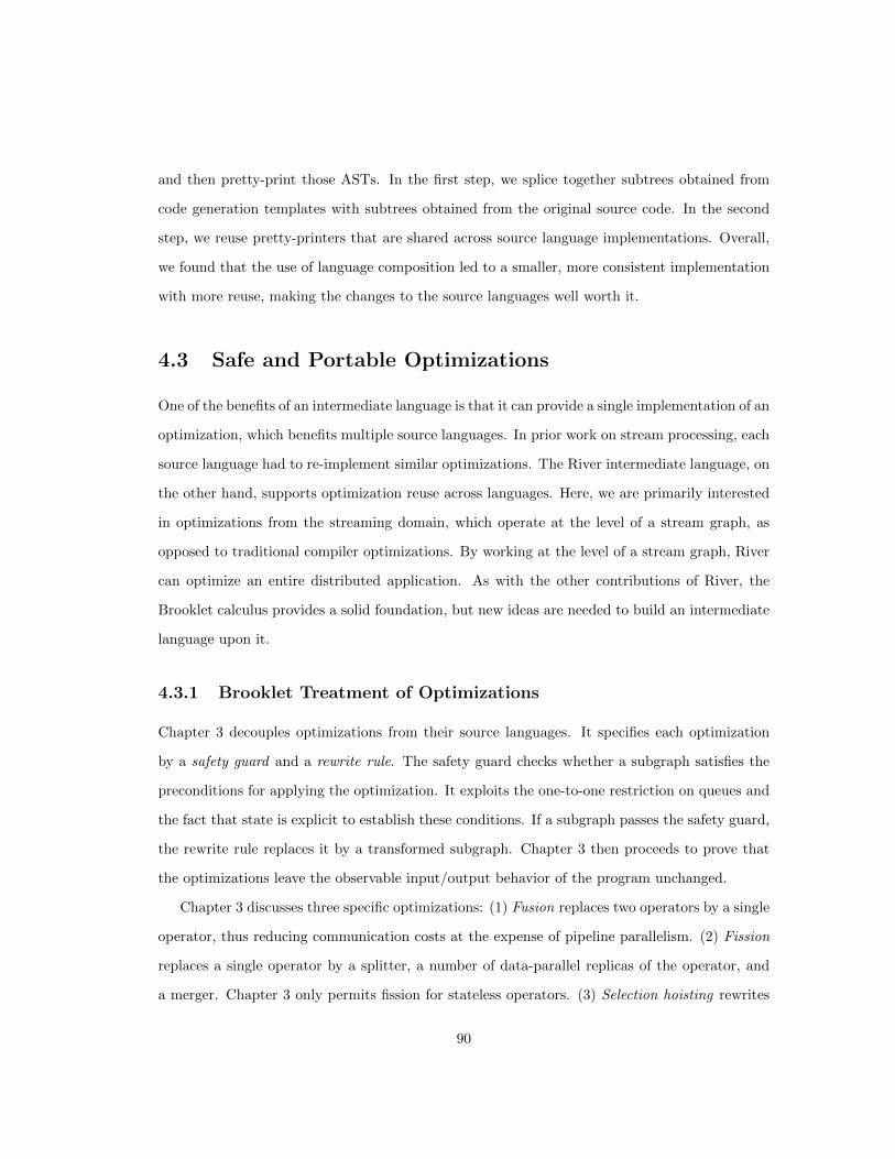
and then pretty-print those ASTs. In the first step, we splice together subtrees obtained from

code generation templates with subtrees obtained from the original source code. In the second

step, we reuse pretty-printers that are shared across source language implementations. Overall,

we found that the use of language composition led to a smaller, more consistent implementation

with more reuse, making the changes to the source languages well worth it.

4.3 Safe and Portable Optimizations

One of the benefits of an intermediate language is that it can provide a single implementation of an

optimization, which benefits multiple source languages. In prior work on stream processing, each

source language had to re-implement similar optimizations. The River intermediate language, on

the other hand, supports optimization reuse across languages. Here, we are primarily interested

in optimizations from the streaming domain, which operate at the level of a stream graph, as

opposed to traditional compiler optimizations. By working at the level of a stream graph, River

can optimize an entire distributed application. As with the other contributions of River, the

Brooklet calculus provides a solid foundation, but new ideas are needed to build an intermediate

language upon it.

4.3.1 Brooklet Treatment of Optimizations

Chapter 3 decouples optimizations from their source languages. It specifies each optimization

by a safety guard and a rewrite rule. The safety guard checks whether a subgraph satisfies the

preconditions for applying the optimization. It exploits the one-to-one restriction on queues and

the fact that state is explicit to establish these conditions. If a subgraph passes the safety guard,

the rewrite rule replaces it by a transformed subgraph. Chapter 3 then proceeds to prove that

the optimizations leave the observable input/output behavior of the program unchanged.

Chapter 3 discusses three specific optimizations: (1) Fusion replaces two operators by a single

operator, thus reducing communication costs at the expense of pipeline parallelism. (2) Fission

replaces a single operator by a splitter, a number of data-parallel replicas of the operator, and

a merger. Chapter 3 only permits fission for stateless operators. (3) Selection hoisting rewrites

90

a subgraph A→ σ into a subgraph σ → A, assuming that A is a stateless operator and σ is a

selection operator that only relies on data fields unchanged by A. Selection hoisting is profitable

if A is expensive and σ reduces the number of data items that A needs to process. Chapter 3

relied on analyzing the function of operator A to establish the safety of selection hoisting.

4.3.2 River Optimization Support

We made the observation that River’s source languages are designed to make certain optimiza-

tions safe by construction, without requiring sophisticated analysis. For example, Sawzall pro-

vides a set of built-in aggregations that are known to be commutative, and partitioned by a

user-supplied key, thus enabling fission. Rather than loosing safety information in translation,

only to have to discover it again before optimization, we wanted to add it to River’s intermediate

language (IL). However, at the same time, we did not want to make the IL source-language

specific, which would jeopardize the reusability of optimizations and the generality of River.

We solved this dilemma by adding extensible annotations to River’s graph language. An

annotation next to an operator specifies policy information, which encompasses safety and prof-

itability. Safety policies are usually passed down by the translator from source language to IL,

such as, which operators to parallelize. Profitability policies usually require some knowledge of

the execution platform, such as the number of machines to parallelize on. In this chapter, we use

simple heuristics for profitability; prior work has also explored more sophisticated analyses for

this, which are beyond the scope of this chapter [46]. Policy is separated from mechanism, which

implements the actual code transformation that performs the optimization. River’s annotation

mechanism allows it to do more powerful optimizations than Brooklet. For example, fission in

River works not just on stateless operators, but also on stateful operators, as long as the state is

keyed and the key fields are listed in annotations. Both CQL and Sawzall are designed explicitly

to make the key evident from the source code, so all we needed to do is preserve that information

through their translators.

To keep annotations extensible, they share a common, simple syntax, inspired by Java. Each

use of an operator is preceded by zero or more annotations. Each annotation is written as an at-

91

sign (@), an identifier naming the annotation, and a comma-separated list of expressions serving

as parameters. In other words, the general annotation syntax is:

operatorUse ::= annotation∗ opOutputs ‘<-’ ID opInputs ‘;’

opOutputs ::= ‘(’ ID (‘,’ ID)∗ ‘)’

opInputs ::= ‘(’ ID (‘,’ ID)∗ ‘)’

annotation ::= ‘@’ ID ‘(’ (expr (‘,’ expr)∗)? ‘)’

River currently makes use of the following annotations:

Annotation Description

@Fuse(ID) Directive to fuse operators with the same ID in the same

process.

@Parallel() Directive to perform fission on an operator.

@Commutative() Declares that an operator’s function is commutative.

@Keys(k1,. . .,kn) Declares that an operator’s state is partitionable by the

key fields k1,. . .,kn in each data item.

@Group(ID) Directive to place operators with the same ID on the same

machine.

We anticipate adding more annotations as we implement more source languages and/or more

optimizations. The translator from River IL to native code invokes the optimizers one by one,

transforming the IL at each step. A specification passed to the translator determines the order

in which the optimizations are applied.

4.3.3 Fusion Optimizer

Intuition. Fusion combines multiple stream operators into a single stream operator, to avoid

the overhead of data serialization and transport [45, 63].

Policy. The policy annotation is @Fuse(ID). Operators with the same ID are fused. Applying

fusion is a tradeoff. It eliminates a queue, reducing communication cost, but it prohibits operators

from executing in parallel. Hence, fusion is profitable if the savings in communication cost exceed

92

the lost benefit of parallelism. As shown in the Brooklet calculus, a sufficient safety precondition

for fusion is if the fused operators form a straight-line pipeline without side entries or exits.

Mechanism. The current implementation replaces internal queues by direct function calls. A

possible future enhancement would be to allow fused operators to share the same process but

run on different threads. This would reduce the cost for communication, but still maintain the

benefits of pipeline parallelism on multi-cores.

4.3.4 Fission Optimizer

Intuition. Fission replicates an operator or a stream subgraph to introduce parallel computa-

tions on subsets of the data [29, 30, 45].

Policy. Fission uses three annotations. The @Parallel() annotation is a directive to parallelize

an operator. The @Commutative() annotation declares that a given operator’s function commutes.

Commutative operators can be safely parallelized because their functions do not depend on the

order of the input data. Finally, the @Keys(k1,. . .,kn) annotation declares that an operator is

stateful, but that its state is keyed (i.e. partitioned) by the key in fields k1,. . .,kn. Fission is

profitable if the computation in the parallel segment is expensive enough to make up for the the

overhead of the inserted split and merge operators. The safety conditions for fission depend on

state and order. In terms of state, there must be no memory dependencies between replicas of the

operator. This is trivially the case when the operator is stateless. The other way to accomplish

this is if the state of the operator can be partitioned by key, such that each operator replica is

responsible for a separate portion of the key space. In that case, the splitter routes data items by

using a hash on their key fields. When a parallel segment consists of multiple operators, they must

be either stateless or have the same key. To understand how order affects correctness, consider

the following example. Assume that in the unoptimized program, the operator pushes data item

d1 before d2 on its output queue. In the optimized program, d1 and d2 may be computed by

different replicas of the operator, and depending on which replica is faster, d2 may be pushed first.

That would be unsafe if any down-stream operator depends on order. That means that fission is

93

safe with respect to order either if all down-stream operators commute, or if the merger brings

data items from different replicas back in the right order. Depending on the source language, the

merger can use different ordering strategies: CQL embeds a logical timestamp in every data item

that induces an ordering; Sawzall has commutative aggregations and can hence ignore order; and

StreamIt only parallelizes stateless operators and can hence use round-robin order.

Mechanism. River’s fission optimization consists of multiple steps. Consider the following

example in which three operators appear in a pipeline. The first two operators, range and aggr,

are stateful, and keyed by k1 and k2 respectively. The third, istream, is stateless. The figures

indicate stateful operators by a rectangle with a folded corner. All three operators have the

@Parallel() annotation, indicating that fission should replicate them.

range aggr istream

@Parallel()@Keys(k1)

@Parallel()@Keys(k2) @Parallel()

Step 1 adds split and merge operators around parallelizable operators. This trivially parallelizes

each individual operator. At the same time, it introduces bottlenecks, as data streamed through

adjacent mergers and splitters must pass through a single machine. Note that for source or

sink operators, only merge or split, respectively, are needed. This is because the partitioning is

assumed to occur outside of the system.

range merge split aggr merge split istream

Step 2 removes the bottlenecks. There are two in the example; each calls for a different action.

First, the merge and split between aggr and istream can be safely removed, because istream is

stateless.

range merge split aggr istream

Next, the merge and split between range and aggr cannot be removed, because both operators

partition state by different keys, k1 and k2. Instead, we apply a rotation. A rotation switches the

order of the merge and split to remove the bottleneck. This is the same approach as the shuffle

94

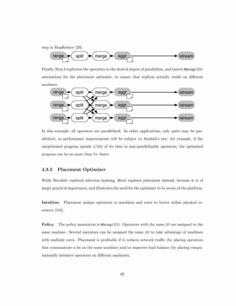
step in MapReduce [29].

range split merge aggr istream

Finally, Step 3 replicates the operators to the desired degree of parallelism, and inserts @Group(ID)

annotations for the placement optimizer, to ensure that replicas actually reside on different

machines.

range split merge aggr istream

range split merge aggr istream

range split merge aggr istream

In this example, all operators are parallelized. In other applications, only parts may be par-

allelized, so performance improvements will be subject to Amdahl’s law: for example, if the

unoptimized program spends 1/5th of its time in non-parallelizable operators, the optimized

program can be no more than 5× faster.

4.3.5 Placement Optimizer

While Brooklet explored selection hoisting, River explores placement instead, because it is of

larger practical importance, and illustrates the need for the optimizer to be aware of the platform.

Intuition. Placement assigns operators to machines and cores to better utilize physical re-

sources [116].

Policy. The policy annotation is @Group(ID). Operators with the same ID are assigned to the

same machine. Several operators can be assigned the same ID to take advantage of machines

with multiple cores. Placement is profitable if it reduces network traffic (by placing operators

that communicate a lot on the same machine) and/or improves load balance (by placing compu-

tationally intensive operators on different machines).

95

Mechanism. The placement mechanism does not transform the IL, but rather, directs the

runtime to assign the same machine to all operators that use the same identifier. Information

such as the number of machines is only available at the level of the intermediate language, a

trait that River shares with other language-based virtual machines. Placement is complicated

if operators share state. In general, River could support sharing variables across machines, but

relies on the underlying runtime to support that functionality. Because our current backend does

not provide distributed shared state, the placement optimizer has an additional constraint. It

ensures that all operators that access the same shared variable are placed on the same machine.

Fortunately, none of the streaming languages we encountered so far need cross-machine shared

state.

4.3.6 When to Optimize

The Brooklet calculus abstracts away the timing of optimizations. In River, optimizations are

applied once the available resources are known, just before running the program. In other words,

the translations from source languages to IL happen ahead of time, but the translation from IL to

native code for a specific target platform is delayed until the program is launched. That enables

River to make more informed profitability decisions. We have not yet taken the next step, which

would be dynamic optimizations that make decisions at runtime. Dynamic optimizations can

use profile information without requiring a separate training run; they can adapt when available

resources change, for example, as the result of failure, or due to another application launched on

the same system; and they can adapt when load characteristics change, for example, based on

the time of day.

A straight-forward approach to dynamic optimizations is to drain all queues in a (sub-)graph

of their in-flight data items, take the (sub-)graph offline, restructure it, and then bring it back

online [4, 57]. This approach is similar to JIT (just-in-time) compilers for traditional optimiza-

tions. However, in the streaming domain, it may be too disruptive, because many streaming

applications are required to produce continuous low-latency outputs.

A more nimble approach to dynamic optimizations is to statically create a more general graph,

96

OS (processes, sockets, …)

Streaming runtime

Runtime adaptation layer

Operators Variables

Call-back mediation

River FFI

(De-)Marshalling

proc

ess(

…)

subm

it(…

)

Figure 4.4: Stack of layers for executing River.

and then adapt how data flows through it at runtime. A seminal example for this is the Eddy

operator, which performs dynamic operator reordering without physically changing the graph at

runtime [12]. While we have not yet implemented optimizations that use this approach, River is

well-suited for it. The approach would use annotations to decide where an optimization applies,

statically rewrite the graph, and add in control operators that dynamically route data items for

optimization.

4.4 Runtime Support

The main goal for River’s runtime support is to insulate the IL and the runtime from each

other. Figure 4.4 shows the architecture. It consists of a stack of layers, where each layer only

knows about the layers immediately below and above it. At the lowest level is the streaming

runtime, which provides the software infrastructure for process management, data transport, and

distribution. Above that is the runtime adaptation layer, which provides the interface between

River operators and the distributed runtime. At the highest level are the operator instances

and their associated variables. River’s clean separation of concerns ensures that it can be easily

ported to additional streaming runtimes. The rest of this section describes each layer in detail.

97

4.4.1 Streaming Runtime

A distributed streaming runtime for River must satisfy the following requirements. It must

launch the right processes on the right machines in the distributed system to host operators

and variables. It must provide reliable transport with ordered delivery to implement queues.

It must arbitrate resources and monitor system health for reliability and performance. Finally,

our placement optimizer relies on placement support in the runtime. There is no strict latency

requirement: the semantics tolerate an indefinite transit time.

The streaming runtime sits on top of an operating system layer, which provides basic cen-

tralized services to the runtime layer, such as processes, sockets, etc. However, building a high-

performance streaming runtime satisfying the above-listed requirements is a significant engineer-

ing effort beyond the OS. Therefore, we reuse an existing runtime instead of building our own.

We chose System S [42], a distributed streaming runtime developed at IBM that satisfies the

requirements, and that is available to universities under an academic license. While System S

has its own streaming language, we bypassed that in our implementation, instead interfacing

with the runtime’s C++ API.

4.4.2 Runtime Adaptation

The runtime adaptation layer provides the interface between River operators and the distributed

runtime. As shown in Figure 4.4, it consists of three sub-layers.

Call-Back Mediation Layer. This layer mediates between the runtime-specific APIs and call-

backs, and the River-specific functions. The code in this layer peels off runtime-specific headers

from a data item, and then passes the data item to the layer above. Similarly, it adds the headers

to data on its way down. If there are shared variables, this layer performs locking, and implements

output buffers for avoiding back-pressure induced dead-lock as described in Section 4.1.4. The

call-back mediation layer is linked into the streaming runtime.

98

River FFI Layer. A foreign function interface, or FFI for short, enables calls across program-

ming languages. In this case, it enables C++ code from a lower layer to call a River function in

an upper layer, and it enables River code in an upper layer to call a C++ function in a lower

layer. The River FFI is the same as the OCaml FFI. Each OS process for River contains an

instance of the OCaml runtime, which it launches during start-up.

(De-)Marshalling Layer. This layer converts between byte arrays and data structures in

River’s implementation language. It uses an off-the-shelf serialization module. The code in this

layer is auto-generated by the River compiler. It consists of process(...) functions, which are

called by the next layer down, demarshal the data, and call the next layer up; and of submit(...)

functions, which are called by the next layer up, marshal the data, and call the next layer down.

Since this layer is crucial for performance, we have plans to optimize it further by specialized

code generation.

4.4.3 Variables and Operators

As described in Section 4.2.4, operators are generated from templates written by the language

developer. We chose to use templates to support operator specialization in River, because they

allow for static syntax checking and do not add to performance overhead. Their implementa-

tion strikes a balance between the functional purity of operators in Brooklet, and performance

demands of a practical IL that needs to update data in place, and make callbacks instead of

returning values. Variables and operators are implemented in the implementation sublanguage

of River. An operator firing takes the form of a function call from the next lower layer. If the

operator accesses variables, then the call passes those as references, so that the operator can

perform in-place updates if needed. Instead of returning data as part of the function’s return

value, the operator invokes a call-back for each data item it produces on an output queue. Note

that this simple API effectively hides any lower-layer details from the variables and operators.

99

4.5 Evaluation

now project

istream

dupsplit

ran ge

join

istream

aggregate

join

se lect

join

ran ge

partition

project

dis tinct

dup-split

now

project

aggregate

pro ject

pro ject

rstream

low- pass

de-mod split

split

low- pass

low- pass

join subtract

join eq-filter

split

low- pass

low- pass

join subtract

(a) CQL’s Linear Road in River. (b) StreamIt’s FM Radio in River.

Figure 4.5: Structural view for the CQL and StreamIt benchmarks, distributed across 4 machineseach for task and pipeline parallelism. The dashed ovals group operators that are placed ontothe same machine.

We have built a proof-of-concept prototype of River, including front-ends for three source

languages, implementations of three optimizations, and a back-end on a distributed streaming

system. We have not yet tuned the absolute performance of our prototype; the goal of this

chapter was to show its feasibility and generality. Therefore, while this section presents some

experimental results demonstrating that the system works and performs reasonably well, we leave

further efforts on absolute performance to future work.

All performance evaluations were run on a cluster of 16 machines. Each machine has two

4-core 64-bit Intel Xeon (X5365) processors running at 3.00GHz, where each core has 32K L1i

and 32K L1d caches of its own, and a 4MB unified L2 cache that is shared with another core.

The processors have a FSB speed of 1,333 MHz and are connected to 16GB of uniform memory.

Machines in the cluster are connected via 1Gbit ethernet.

4.5.1 Support for Existing Languages

To verify that River is able to support a diversity of streaming languages, we implemented the

language translators described in Section 4.2, as well as illustrative benchmark applications. The

benchmarks exercise a significant portion of each language, demonstrating the expressivity of

River. They are described below:

100

CQL Linear Road. Linear Road [8] is a benchmark designed by the authors of CQL. It is a

hypothetical application that computes tolls for vehicles traveling on the Linear Road highway.

(Figure 4.5 (a) shows the operator graph of the application.) Each vehicle is assigned a unique

ID, and its location is specified by three attributes: speed, direction, and position. Each highway

in also assigned an ID. Vehicles pay a toll when they drive on a congested highway. A highway

is congested if the average speed of all vehicles on the highway over a 5 minute span is less than

40 mph.

StreamIt FM Radio. This benchmark implements a multi-band equalizer [45]. As shown in

Figure 4.5 (b), the input passes through a demodulator to produce an audio signal, and then an

equalizer. The equalizer is implemented as a splitjoin with two band-pass filters; each band-pass

filter is the difference of a pair of low-pass filters.

Sawzall Batch Log Analyzer. Figure 4.2 (d) shows this query, which is based on an exemplar

Sawzall query in Pike et al. [93]. It is a batch job that reads its input from the distributed file

system. The program analyzes a set of search query logs to count queries per origin based on IP

address. The resulting aggregation could then be used to plot query origins on a world map.

CQL Continuous Log Analyzer. This is similar to the Sawzall log query analyzer, but it

is a continuous query rather than a batch job. Its input comes from a server farm. Each server

reports the origin of the requests it has received, and the analyzer performs an aggregation keyed

by the origin over the most recent 5 minute window. Note that the data is originally partitioned

by the target (server) address, so the application must shuffle the data.

The benchmark applications exercise significant portions of each language. This demonstrates

that River is flexible enough to express three source languages, CQL, StreamIt, and Sawzall, that

occupy diverse points in the design space for streaming languages.

101

4.5.2 Suitability for Optimizations

To verify that River is extensible enough to support a diverse set of streaming optimizations, we

implemented each of the optimizations described in Section 4.3. We then applied the different

optimizations to the benchmark applications from Section 4.5.1.

Placement. Our placement optimizer distributes an application across machines. Operators

from each application were assigned to groups, and each group was executed on a different

machine. As a first step, we used the simple heuristic of assigning operators to groups according

to the branches of the top-level split-merge operators, although there has been extensive prior

work [116] on determining the optimal assignments. In the non-fused version, each operator had

its own process, and it was up to the OS to schedule processes to cores. Figure 4.6 (a) and (b)

show the results of running both Linear Road and the FM Radio applications on 1, 2, and 4

machines. These experiments demonstrate that distribution improves applications performance.

Figure 4.5 shows the partitioning scheme for the 4-machine case using dashed ovals. These

results are particularly exciting because the original implementation of CQL was not distributed.

Despite the fact that the Linear Road application shows only limited amounts of task and pipeline

parallelism, the first distributed CQL implementation achieves a 3.70× speedup by distributing

execution on 4 machines. The FM Radio application exhibits a 1.84× speedup on 4 machines.

Fission. Our fission optimizer replicates operators, and then distributes those replicas evenly

across available machines. We tested two applications, the Sawzall batch log analyzer and the

CQL continuous log analyzer, with increasing amounts of parallelism. In these experiments,

the degree of parallelism corresponded to the number of available machines, from 1 to 16. We

additionally ran the Sawzall query on 16 machines with 16, 32, 48, and 64 degrees of parallelism,

distributing the computation across cores. The results are shown in Figures 4.6 (c) and (d).

Fission adds split and merge operators to the stream graph. Therefore, in the non-fissed case,

there are fewer processing steps. Despite of this, the Sawzall program’s throughput increased

when the degree of parallelism went from 1 to 2. As the degree of parallelism and the number of

102

1.00

2.63 3.70

0.67

1.60

4.02

0.1

1.0

10.0

1 2 4

Speedup: Linear road

No fusion Fusion

1.00

1.32

0.93

0.67 0.80

1.01

0.0

1.0

2.0

1 2 4

Scaleup: Linear road

No fusion Fusion

(a) Linear Road.

1.00

1.48 1.84

1

10

1 2 4

Speedup: FM radio

1.00

0.74

0.46

0.0

0.2

0.4

0.6

0.8

1.0

1.2

1 2 4

Scaleup: FM radio

(b) FM Radio.

1.28

2.53

4.94 8.92

16.02 14.80

2.06

4.28

8.26

16.95

31.95 50.32

1

10

100

1 2 4 8 16 32 64

Speedup: Batch log analyzer

No fusion Fusion 1.00

0.64 0.63 0.62 0.56 0.50

0.23

1.03 1.07 1.03 1.061.00

0.79

0.0

0.2

0.4

0.6

0.8

1.0

1.2

1 2 4 8 16 32 64

Scaleup: batch log analyzer

No fusion Fusion

(c) Batch log analyzer.

1.00

1.88 2.16 2.19 2.14

1

10

1 2 4 8 16

Speedup: Continuous log analyzer

1.00 0.94

0.54

0.27 0.13

0.0

0.2

0.4

0.6

0.8

1.0

1.2

1 2 4 8 16

Scaleup: Continuous log analyzer

(d) Continuous log analyzer.

Figure 4.6: Speedup is the throughput relative to single machine. Scaleup is the speedup dividedby number of machines in (a) and (b), and the speedup divided by the degree of parallelism in(c) and (d).

machines increased from 2 to 16, the increase in throughput was linear, with an 8.92× speedup

on 16 machines. When further distributed across cores, the Sawzall program also experience a

103

large performance increase. However, the 32 replicas case showed better performance than 64

replicas. This makes sense, since the unfused Sawzall query has 5 operators, each of which was

replicated 64 times (64 ∗ 5 = 320), while the total number of available cores across all machines

was 16 ∗ 8 = 128.

The CQL continuous log analyzer saw a performance improvement with fission, but only

achieved at best a 2.19× speedup, with no benefit past 6 machines. Unlike Sawzall, all data

items in CQL are timestamped. To maintain CQL’s deterministic semantics, mergers must wait

for messages from all input ports for a given timestamp. The lesson we learned was that when

implementing a distributed, data-parallel CQL, we need to give more consideration to how to

enforce deterministic execution efficiently. Unlike our River-CQL implementation, the original

CQL did not do fission and thus did not encounter this issue.

Fusion. The Linear Road results in Figure 4.6 (a) illustrate the tradeoffs during fusion, which

often comes at the expense of pipeline parallelism. The fusion optimization only improves per-

formance in the 4-machine case, where it achieves a 4.02× speedup, which is overall better than

the 4-machine results without fusion. Figure 4.6 (c) shows that fusion is particularly beneficial

to the Sawzall log query analyzer. In this case, fusion eliminates much of the per-data item

processing overhead, and therefore allows the fission optimization to yield much better results.

Fusion combines each mapper with its splitter and each reducer with its merger. With both fu-

sion and fission, the Sawzall log query analyzer speeds up 50.32× on 16 machines with 64 degrees

of parallelism.

Calibration to Native Implementation. The placement, fission, and fusion optimizations

demonstrate that River can support a diverse set of streaming optimizations, thus validating our

design. While we did not focus our implementation efforts on absolute performance metrics, we

were interested to see how River’s performance compared to a native language implementation.

Native Sawzall programs are translated to MapReduce jobs. We therefore implemented the

Sawzall web log analyzer query as a Hadoop job. We ran both Hadoop and River on a cluster of

16 machines, with an input set of 109 data items, around 24GB. Hadoop was able to process this

104

data in 96 seconds. We observed that the Hadoop job started 92 mappers during its execution,

so we ran River with 92 mappers, and computed the results in 137 seconds. However, we should

point out that the execution model for both systems differs. While Hadoop is a batch processing

system and stores its intermediate results to disk, River is a streaming system, in which the

mapper and the reducer are running in parallel, and intermediate results are kept in memory.

Given that there are 16 machines with 8 cores each, we ran River again with 64 mappers and 64

reducers (16 ∗ 8 = 64 + 64 = 128). Under this scenario, River completed the computation in 115

seconds.

Despite the fact that Hadoop is a well-established system that has been heavily used and

optimized, the River prototype ran about 83% as fast. There are two reasons for this performance

difference. First, our current fission optimizer always replicates the same number of mappers as

reducers, which may not be an optimal configuration. Additional optimization work is needed to

adjust the map-to-reduce ratio. Second, our implementation has some unnecessary serialization

overheads. A preliminary investigation suggests that eliminating those would give us performance

on par with Hadoop.

4.5.3 Concurrency

This section explores the effectiveness of the locking algorithm from Figure 4.1.

Coarse-Grained Locking. For the coarse-grained locking experiment, we used the following

setup, described in River’s topology language:

(q2, $v1) <- f1(q1, $v1 );

(q3, $v1, $v2) <- f2(q2, $v1, $v2);

(q4, $v2) <- f3(q3, $v2);

In this example, f1 and f3 are expensive (implemented by sleeping for a set time), whereas f2 is

cheap (implemented as the identity function). Operator instances f1 and f2 share the variable

$v1, and f2 and f3 share the variable $v2. With naive locking, we would put all three variables

under a single lock. That means that all three operator instances are mutually exclusive, and

105

2.2

20.5

235.1

2,833.9

4.2

40.2

400.2

3,999.8

1

10

100

1,000

10,000

0.001 0.01 0.1 1

Tim

e [s

]

Delay [s]

Coarse locking experiment

One lock Two locks

0

100

200

300

400

0 250 500 750 1000 1250

Tim

e [s

]

Number of locks

Fine locking experiment

(a) Coarse locking (b) Fine locking

Figure 4.7: Locking experiments

you would expect the total execution time to be approximately:

cost(f1) + cost(f2) + cost(f3)

On the other hand, with our smarter locking scheme, f1 and f3 have no locks in common and

can therefore execute in parallel. Hence, you would expect an approximate total execution time

of:

max{cost(f1), cost(f3)}+ cost(f2)

We tested this by varying the cost (i.e. delay) of the operators f1 and f3 over a range of 0.001

to 1 seconds. The results, in Figure 4.7 (a), behave as we expected, with our locking scheme

performing approximately twice as fast as with the naive version.

Fine-Grained Locking. As a second micro-benchmark for our locking algorithm, we wanted

to quantify the overhead of locking on a fine-grained level. We used the following setup, described

in River’s topology language:

(q2, $v1, ..., $vn) <- f1(q1, $v1, ..., $vn);

(q3, $v1, ..., $vn) <- f2(q2, $v1, ..., $vn);

Operators f1 and f2 share variables $v1 . . . $vn, where we incremented n from 1 to 1,250. With

naive locking, each variable would be protected by its own lock, as opposed to our locking scheme,

which protects all n variables under a single lock. Figure 4.7 (b) shows that the overhead of the

naive scheme grows linearly with the number of locks.

106

4.6 Chapter Summary

This chapter presents River, an intermediate language for distributed stream processing. River

is founded on the Brooklet calculus. Stream processing is widely used, easy to distribute, and

has language diversity. By providing an intermediate language for streaming, we are making

a lot of common infrastructure portable and reusable, and thus facilitating further innovation.

And by building our intermediate language on a calculus, we are giving a clear definition of how

programs should behave, thus enabling reasoning about correctness.

One contributions of this chapter is to show how to maintain the properties of the calculus in

the intermediate language. The Brooklet calculus has a small-step operational semantics, which

models execution as a sequence of atomic operator firings using pure functions. In River, operator

firings still behave as if atomic, but are concurrent and do not need to be pure.

A second contribution of this chapter is to make source language development economic. We

show how to reuse common language components across diverse languages, thus limiting the effort

of writing parsers, type checkers, and code generators to the unique features of each language.

The River intermediate language includes an intermediate language for describing stream graphs

and operator implementations. We use code generation for operator implementations based on

a simple templating mechanism.

A third contribution of this chapter is to provide safe optimizations that work across different

source languages. Each source language is designed to make the safety of certain optimizations

evident. We provide an annotation syntax, so that on the one hand, translators from the source

languages can retain the safety information, while on the other hand, optimizers can work at the

IL level without being source-language specific. Each optimizer uses the annotations as policy

and implements the program manipulation as mechanism.

To conclude, River is an intermediate language for running multiple streaming languages on a

distributed system, and comes with an eco-system for making it easy to implement and optimize

multiple source-languages. River is based on a calculus, giving it a clear semantics and strong

correctness guarantees.

107

5

Related Work

5.1 Streaming Languages

Stream processing has a long history in computer science. This thesis primarily uses CQL [8],

Sawzall [93], and StreamIt [112] as representative examples of streaming languages, but there

are many more. Prominent early examples include Signal [15] and Lustre [51], which, like StreamIt,

explore a synchronous programming model. Spade [42] and it successor SPL [54] are streaming

languages for composing parallel and distributed flow graphs for System S, IBM’s scalable data

processing middleware. Gigascope [28] is a lightweight streaming database designed for net-

work monitoring and analysis. It is programmed with GSQL, a query language with SQL-like

syntax. Hancock [27] is a query language designed for data-mining in the telecommunications

domain. Pig Latin [88] is one of the languages designed to compose MapReduce or Hadoop jobs.

DryadLINQ [123] runs imperative code on local machines and uses integrated SQL to generate

distributed queries. Several languages, including Brook [19], CUDA [86], and OpenCL [64] are

targeted at programming GPUs.

5.2 Surveys on Stream Processing

Chapter 2 presents a catalog of stream processing optimizations. Existing surveys on stream

processing do not focus on optimizations [106, 13, 61], and existing catalogs of optimizations

do not focus on stream processing. Chapter 2 provides both. The presentation is inspired by

catalogs for design patterns [40] and for refactorings [38].

5.3 Semantics of Stream Processing

Chapter 3 presents the Brooklet calculus. Brooklet takes inspiration from Featherweight Java [59],

in that they both define core minimal languages that allow us to reason about correctness. There

108

has been extensive prior work in the semantics of stream processing. Brooklet is designed

to facilitate reasoning about language and optimization implementation in distributed systems,

and therefore chooses different abstractions from other formalisms. Notably, the π-calculus does

not model state [79]. The ambient calculus omits state and makes computations mobile [22].

Kahn process networks [62], such as Unix pipes, assume deterministic execution. Synchronous

data flow [70] models, such as StreamIt, assume fixed buffer sizes and static communication

patterns. Hoare’s communicating sequential process [56] assumes no buffering, and synchronous

communication. Finally, Gurevich et al. present an abstract formalism without state and com-

munications [50].

5.4 Continuous Queries

The database literature often refers to streaming applications as continuous queries [25, 109].

Surprisingly, there is little work from the database community on optimizations of queries with

side effects. Two exceptions are a study of XQuery with side effects [43] and a study of object-

oriented databases [35].

5.5 Intermediate Language for Streaming

Chapter 4 presents River, an intermediate language for streaming, which runs on a dis-

tributed system and supports multiple source languages. SVM, the stream virtual machine, is a

C framework for streaming on both CPU and GPU back-ends, but the paper does not describe

any source-language support [66]. MSL, the multicore streaming layer, executes the StreamIt

language on the Cell architecture [124]. Erbium is a set of intrinsic functions for a C compiler for

streaming on an x86 SMP, but the paper describes no source-language support [80]. And Lime is

a new streaming language with three back-ends: Java, C, and FPGA bit-files [11]. None of SVM,

MSL, Erbium, or Lime are distributed on a cluster, none of them are founded on a calculus, and

they all have at most a single source language each. While we are not aware of prior work on

intermediate languages for distributed streaming, there are various execution environments for

109

distributed batch dataflow. MapReduce [29] has emerged as a de-facto execution environment for

various batch-processing languages, including Sawzall [93], Pig Latin [88], and FlumeJava [24].

Dryad [60] is a batch execution environment that comes with its own language Nebula, but is

also targeted by DryadLINQ [123]. CIEL is a batch execution environment with its own language

SkyWriting [84]. Like MapReduce, Dryad, and CIEL, River runs on a shared-nothing cluster,

but unlike those works, River is designed for continuous streaming, and derived from a calculus.

5.6 Economic Source-Language Development

River comes with an eco-system for economic source-language development. The LINQ

framework (language integrated query) also facilitates front-end implementation, but using a

different approach: LINQ embeds SQL-style query syntax in a host language such as C#, and

targets different back-ends such as databases or Dryad [76]. Our approach follows more traditional

compiler frameworks such as Polyglot [87] or MetaBorg [17]. We use the Rats! parser generator

to modularize grammars [48]. Our approach to modularizing type-checkers and code-generators

uses the same approach as Jeannie [55], but River composes more language components at a finer

granularity.

5.7 Streaming Optimizations

Several communities have come up with similar streaming optimizations, but unlike River,

they do not decouple the optimizations from the source-language translator and reuse them across

different source languages. In parallel databases [30], the IL is relational algebra. Similarly to

the fission optimization in this paper, parallel databases use hash-splits for parallel execution.

But to do so, they rely on algebraic properties of a small set of built-in operators, unlike River,

which supports an unbounded set of user-defined operators. There has been surprisingly little

work on generalizing database optimizations to the more general case [35, 43], and that work

is still limited to the database domain. The StreamIt compiler implements its own variant of

fission [45]. It relies on fixed data rates and stateless operators for safety, and indeed, the StreamIt

110

language is designed around making those easy to establish. Our fission is more general, since

it can parallelize even in the presence of state. MapReduce has data-parallelism hard-wired into

its design. Safety relies on keys and commutativity, but those are up to the user or a higher-

level language to establish. River supports language-independent optimization by making such

language-specific safety properties explicit in the IL.

111

6

Limitations and Future Work

There are three components to this thesis: a catalog of stream processing optimizations; the

Brooklet calculus for stream processing; and the River intermediate language. Taken collectively,

these components provide a reusable infrastructure for stream processing languages. However,

this thesis does not address all the needs for stream processing with regards to infrastructure

support. This chapter identifies some of the limitations and key avenues for future work for each

of the three components, primarily the support for dynamic optimizations.

Optimizations Catalog. As a survey of the most prominent streaming optimizations, this

chapter is fairly conprehensive. However, it also offers some broader observations, and proposes

several avenues for future research. Since they have already been discussed in detail, we only list

the proposals here with references to the relevant sections. The avenues for future work include:

further study on how to augment languages to support optimization (§ 2.12.1); determining the

best order for applying optimizations (§ 2.12.2); new compiler analysis for enabling optimiza-

tions (§ 2.12.3); extending existing optimizations beyond their current restrictions (§ 2.12.5);

exploring how to support dynamic optimizations (§ 2.12.4); and defining standard benchmarks

for streaming (§ 2.12.6).

Brooklet. There are many formal models for streaming systems [9, 62, 68, 70]. Additional

work is needed to formalize the relationship between Brooklet and these other process calculi.

For example, by mapping (if possible) a Brooklet program to the π-calculus [79] or the actor

model [53], and vice-versa.

Many streaming applications have time constraints. In healthcare, there might be real-time

constraints for reporting critical events. In finance, trades might need to happen within a certain

time window. For streaming media applications, there might be limits on latency to ensure

stutter free playback. Brooklet does not have a way to formalize these time constraints in the

calculus, but it would clearly be useful for implementing real systems.

112

Chapter 2 surveys eleven prominent streaming optimizations. So far, we have only formalized

three of them using Brooklet. More work is needed to formalize the remaining ones. One

challenge, as discussed in Section 2.13, is that information about non-determinism, state, and

communication is not sufficient to model all of the optimizations in the catalog. We addressed

this problem in the River IL with the use of extensible annotations. How to address this in the

calculus remains an open question.

Section 2.13 also identifies support for dynamic optimization as one of the requirements for a

streaming IL. This is one of the major limitations for both Brooklet and River. We discuss this

in more detail below.

River. River is currently limited in that it only supports static optimizations i.e., those that are

performed before execution. These optimizations are easily modelled as translations from IL to

IL. Dynamic optimizations, i.e., those that are performed during execution, are somewhat more

challenging. One solution would be a global optimization engine, which observes all running

operators across all system nodes and then modifies the operator graph and its mapping to

machines in order to achieve its performance goals. While certainly feasible, this approach

introduces another large component into the architecture. Furthermore, that component would

need to coordinate across all nodes in the system.

A better way to address this limitation would be to take a cue from previous work [3, 12,

99] and, as much as possible, implement dynamic optimizations as operators. Such optimizing

operators are statically injected into an application and then dynamically change the application

by re-routing data or modifying operators and their placement. In effect, the stream processing

application becomes self-monitoring and self-adjusting.

Another limitation of River is its performance. Although the system works and the optimiza-

tions demonstrate improvements in relative performance, the absolute performance is still short of

expectations. Performance could be improved by using a different implementation sublanguage;

by using better serialization; and by implementing a larger set of optimizations.

Finally, we have used River as the target for dialects of three existing streaming languages,

letting their requirements guide the design of the IL. In the future, we would like to leverage our

113

experience with translating front-ends and implementing optimizations into the design of a new

streaming language from scratch using River. This would close the feedback loop, allowing the

IL to guide the design of the language.

114

7

Conclusion

This thesis explores how to provide a reusable infrastructure for stream processing. Stream pro-

cessing applications have become ubiquitous and essential to a variety of application domains,

including entertainment, finance, and healthcare. They are the product of a paradigm shift

towards data-centric applications that are expected to run on multiple processors or multiple

machines. This paradigm shift has a profound impact on the design of both programming lan-

guages and optimizations. In order to support continued innovation in streaming languages and

optimizations, language implementors need the proper infrastructure. Unfortunately, existing

ILs are ill-suited for stream processing, so an intermediate language for stream processing does

not exist.

This thesis has three components. A catalog of stream processing optimizations identifies

what information a streaming IL needs to provide in order to support streaming optimizations.

The Brooklet calculus provides a formal semantics that is general enough to express a wide range

of streaming languages, and enables reasoning about language implementation and optimization

correctness on distributed systems. Finally, the River IL builds on Brooklet by addressing the

real-world details that the calculus elides. The result is a practical intermediate language with a

rigorously defined semantics.

We evaluated our system by implementing front-ends for three diverse streaming languages

(CQL, StreamIt, and Sawzall), and three important optimizations (operator fusion, fission, and

placement). Additionally, we wrote a back-end for River on the System S distributed streaming

runtime. We measured the performance improvements for benchmark applications written in

the streaming languages when the three optimizations were applied. River effectively decouples

the optimizations from the language front-ends, and thus makes them reusable across front-ends,

reducing the overall implementation effort for language implementors.

Finally, this dissertation has suggested directions for future work in regards to infrastructure

support for stream processing. Most importantly, we advocate further research in how to support

dynamic optimizations, which can better take advantage of information only available at runtime,

115

and the design of new streaming languages that are better suited to make use of the support

that the infrastructure provides.

Collectively, these contributions demonstrate that an intermediate language designed to meet

the requirements of stream processing can serve as a common substrate for critical optimizations;

assure implementation correctness; and reduce overall implementation effort. Overall, this work

enables further advances in language and optimization design, and encourages innovation in the

vital domain of stream processing.

116

Bibliography

[1] PoweredBy wiki. Hadoop. http://wiki.apache.org/hadoop/PoweredBy.

[2] Data, data everywhere. The Economist, Feb. 2010. Available from http://www.

economist.com/node/15557443.

[3] D. J. Abadi, Y. Ahmad, M. Balazinska, U. Cetintemel, M. Cherniack, J.-H. Hwang,

W. Lindner, A. S. Maskey, A. Rasin, E. Ryvkina, N. Tatbul, Y. Xing, and S. Zdonik.

The design of the Borealis stream processing engine. In Proc. Conference on Innovative

Data Systems Research, pp. 277–289, Jan. 2005.

[4] D. J. Abadi, D. Carney, U. Cetintemel, M. Cherniack, C. Convey, S. Lee, M. Stonebraker,

N. Tatbul, and S. Zdonik. Aurora: A new model and architecture for data stream man-

agement. The VLDB Journal, 12(2):120–139, Aug. 2003.

[5] G. Aigner, A. Diwan, D. L. Heine, M. S. Lam, D. L. Moore, B. R. Murphy, and C. Sapuntza-

kis. An overview of the SUIF2 compiler infrastructure. Tech. report, Stanford University,

2000.

[6] L. Amini, H. Andrade, R. Bhagwan, F. Eskesen, R. King, P. Selo, Y. Park, and C. Venka-

tramani. SPC: A distributed, scalable platform for data mining. In Proc. 4th International

Workshop on Data Mining Standards, Services, and Platforms, pp. 27–37, Aug. 2006.

[7] L. Amini, N. Jain, A. Sehgal, J. Silber, and O. Verscheure. Adaptive control of extreme-scale

stream processing systems. In Proc. 26th IEEE International Conference on Distributed

Computing Systems, pp. 71–79, July 2006.

[8] A. Arasu, S. Babu, and J. Widom. The CQL continuous query language: Semantic foun-

dations and query execution. The VLDB Journal, 15(2):121–142, June 2006.

[9] A. Arasu and J. Widom. A denotational semantics for continuous queries over streams and

relations. ACM SIGMOD Record, 33(3):6–11, Sept. 2004.

117

[10] R. H. Arpaci-Dusseau, E. Anderson, N. Treuhaft, D. E. Culler, J. M. Hellerstein, D. Pat-

terson, and K. Yellick. Cluster I/O with River: Making the fast case common. In Proc.

6th Workshop on I/O in Parallel and Distributed Systems, pp. 10–22, May 1999.

[11] J. Auerbach, D. F. Bacon, P. Cheng, and R. Rabbah. Lime: A Java-compatible and syn-

thesizable language for heterogeneous architectures. In Proc. ACM Conference on Object-

Oriented Programming Systems, Languages, and Applications, pp. 89–108, Oct. 2010.

[12] R. Avnur and J. M. Hellerstein. Eddies: Continuously adaptive query processing. In ACM

SIGMOD International Conference on Management of Data, pp. 261–272, June 2000.

[13] B. Babcock, S. Babu, M. Datar, R. Motwani, and J. Widom. Models and issues in data

stream systems. In Proc. 21st ACM Symposium on Principles of Database Systems, pp.

1–16, June 2002.

[14] B. Babcock, M. Data, and R. Motwani. Load shedding for aggregation queries over data

streams. In Proc. 20th International Conference on Data Engineering, pp. 350–361, Mar.

2004.

[15] A. Benveniste and P. Le Guernic. Hybrid dynamical systems theory and the SIGNAL

language. IEEE Transactions on Automatic Control, 35(5):535–546, May 1990.

[16] R. D. Blumofe, C. F. Joerg, B. C. Kuszmaul, C. E. Leiserson, K. H. Randall, and Y. Zhou.

Cilk: An efficient multithreaded runtime system. In Proc. 5th ACM SIGPLAN Symposium

on Principles and Practice of Parallel Programming, pp. 207–216, Aug. 1995.

[17] M. Bravenboer and E. Visser. Concrete syntax for objects. In Proc. ACM Conference

on Object-Oriented Programming Systems, Languages, and Applications, pp. 365–383, Oct.

2004.

[18] A. Brito, C. Fetzer, H. Sturzrehm, and P. Felber. Speculative out-of-order event processing

with software transaction memory. In Proc. 2nd International Conference on Distributed

Event-Based Systems, pp. 265–275, July 2008.

118

[19] I. Buck, T. Foley, D. Horn, J. Sugerman, K. Fatahalian, M. Houston, and P. Hanrahan.

Brook for GPUs: Stream computing on graphics hardware. In Proc. ACM International

Conference on Computer Graphics and Interactive Techniques, pp. 777–786, Aug. 2004.

[20] K. Burchett, G. H. Cooper, and S. Krishnamurthi. Lowering: A static optimization tech-

nique for transparent functional reactivity. In Proc. ACM SIGPLAN Symposium on Partial

Evaluation and Semantics-Based Program Manipulation, pp. 71–80, Jan. 2007.

[21] K. Burchett, G. H. Cooper, and S. Krishnamurthi. Lowering: a static optimization tech-

nique for transparent functional reactivity. In Partial Evaluation and Semantics-Based

Program Manipulation (PEPM), pp. 1–80, 2007.

[22] L. Cardelli and A. D. Gordon. Mobile ambients. In Foundations of Software Science and

Computational Structures, vol. 1378 of Lecture Notes in Computer Science, pp. 140–155.

Apr. 1998.

[23] D. Carney, U. Cetintemel, A. Rasin, S. Zdonik, M. Cherniack, and M. Stonebraker. Oper-

ator scheduling in a data stream manager. In Proc. 29th International Conference on Very

Large Data Bases, pp. 838–849, Sept. 2003.

[24] C. Chambers, A. Raniwala, F. Perry, S. Adams, R. R. Henry, R. Bradshaw, and N. Weizen-

baum. FlumeJava: Easy, efficient data-parallel pipelines. In Proc. ACM Conference on

Programming Language Design and Implementation, pp. 363–375, June 2010.

[25] J. Chen, D. J. DeWitt, F. Tian, and Y. Wang. NiagaraCQ: A scalable continuous query

system for internet databases. In Proc. ACM SIGMOD International Conference on Man-

agement of Data, pp. 379–390, May 2000.

[26] T. Condie, N. Conway, P. Alvaro, and J. M. Hellerstein. MapReduce online. In Proc.

7th ACM/USENIX Symposium on Networked Systems Design and Implementation, pp.

313–328, Apr. 2010.

119

[27] C. Cortes, K. Fisher, D. Pregibon, A. Rogers, and F. Smith. Hancock: A language for

analyzing transactional data streams. ACM Transactions on Programming Languages and

Systems, 26(2):301–338, Mar. 2004.

[28] C. Cranor, T. Johnson, O. Spataschek, and V. Shkapenyuk. Gigascope: A stream database

for network applications. In Proc. ACM SIGMOD International Conference on Manage-

ment of Data, pp. 647–651, June 2003.

[29] J. Dean and S. Ghemawat. MapReduce: Simplified data processing on large clusters.

In Proc. 6th USENIX Symposium on Operating Systems Design and Implementation, pp.

137–150, Dec. 2004.

[30] D. DeWitt and J. Gray. Parallel database systems: The future of high performance database

systems. Communications of the ACM, 35(6):85–98, June 1992.

[31] D. J. DeWitt, S. Ghandeharizadeh, D. A. Schneider, A. Bricker, H.-I. Hsiao, and R. Ras-

mussen. The Gamma database machine project. IEEE Transactions on Knowledge and

Data Engineering, 2(1):44–62, Mar. 1990.

[32] Y. Diao, P. Fischer, M. J. Franklin, and R. To. YFilter: Efficient and scalable filtering

of XML documents. In Proc. 18th International Conference on Data Engineering, pp.

341–342, Feb. 2002.

[33] F. Douglis and J. Ousterhout. Transparent process migration: Design alternatives and the

Sprite implementation. Software: Practice and Experience, 21(8):757–785, Aug. 1991.

[34] M. Drake, H. Hoffmann, R. Rabbah, and S. Amarasinghe. MPEG-2 decoding in a stream

programming language. In Proc. 20th IEEE International Parallel and Distributed Pro-

cessing Symposium, pp. 86–95, Apr. 2006.

[35] L. Fegaras. Optimizing queries with object updates. Journal of Intelligent Information

Systems, 12(2–3):219–242, Mar. 1999.

120

[36] J. Ferrante, K. J. Ottenstein, and J. D. Warren. The program dependence graph and its use

in optimization. ACM Transactions on Programming Languages and Systems, 9(3):319–

349, July 1987.

[37] C. L. Forgy. Rete: A fast algorithm for the many pattern/many object pattern match

problem. Artificial Intelligence, 19(1):17–37, Sept. 1982.

[38] M. Fowler, K. Beck, J. Brant, W. Opdyke, and D. Roberts. Refactoring: Improving the

Design of Existing Code. Addison-Wesley, July 1999.

[39] M. Frigo. A fast Fourier transform compiler. In Proc. ACM Conference on Programming

Language Design and Implementation, pp. 169–180, May 1999.

[40] E. Gamma, R. Helm, R. Johnson, and J. Vlissides. Design Patterns: Elements of Reusable

Object-Oriented Software. Addison-Wesley, Jan. 1995.

[41] H. Garcia-Molina, J. D. Ullman, and J. Widom. Database Systems: The Complete Book.

Prentice Hall, second edition, June 2008.

[42] B. Gedik, H. Andrade, K.-L. Wu, P. S. Yu, and M. Doo. SPADE: The System S declarative

stream processing engine. In Proc. ACM SIGMOD International Conference on Manage-

ment of Data, pp. 1123–1134, June 2008.

[43] G. Ghelli, N. Onose, K. Rose, and J. Simeon. XML query optimization in the presence of

side effects. In Proc. ACM SIGMOD International Conference on Management of Data,

pp. 339–352, June 2008.

[44] A. Ghoting, R. Krishnamurthy, E. Pednault, B. Reinwald, V. Sindhwani, S. Tatikonda,

Y. Tian, and S. Vaithyanathan. SystemML: Declarative machine learning on MapReduce.

In Proc. 27th International Conference on Data Engineering, pp. 231–242, Apr. 2011.

[45] M. I. Gordon, W. Thies, and S. Amarasinghe. Exploiting coarse-grained task, data, and

pipeline parallelism in stream programs. In Proc. 12th ACM International Conference on

Architectural Support for Programming Languages and Operating Systems, pp. 151–162,

Oct. 2006.

121

[46] M. I. Gordon, W. Thies, M. Karczmarek, J. Lin, A. S. Meli, A. A. Lamb, C. Leger, J. Wong,

H. Hoffmann, D. Maze, and S. Amarasinghe. A stream compiler for communication-exposed

architectures. In Proc. 10th ACM International Conference on Architectural Support for

Programming Languages and Operating Systems, pp. 291–303, Dec. 2002.

[47] G. Graefe. Encapsulation of parallelism in the Volcano query processing system. In Inter-

national Conference on Management of Data (SIGMOD), pp. 102–111, 1990.

[48] R. Grimm. Better extensibility through modular syntax. In Proc. ACM Conference on

Programming Language Design and Implementation, pp. 38–51, June 2006.

[49] R. Grimm, J. Davis, E. Lemar, A. MacBeth, S. Swanson, T. Anderson, B. Bershad, G. Bor-

riello, S. Gribble, and D. Wetherall. System support for pervasive applications. ACM

Transactions on Computer Systems, 22(4):421–486, Nov. 2004.

[50] Y. Gurevich, D. Leinders, and J. Van Den Bussche. A theory of stream queries. In Proc.

11th International Conference on Database Programming Languages, vol. 4797 of Lecture

Notes in Computer Science, pp. 153–168, Sept. 2007.

[51] N. Halbwachs, P. Caspi, P. Raymond, and D. Pilaud. The synchronous dataflow program-

ming language lustre. 79(9):1305–1320, 1991.

[52] J. Hamilton. Language integration in the common language runtime. ACM SIGPLAN

Notices, 38(2):19–28, Feb. 2003.

[53] C. Hewitt, P. Bishop, and R. Steiger. A universal modular ACTOR formalism for artificial

intelligence. In Proc. 3rd International Joint Conference on Artificial Intelligence, pp.

235–245, 1973.

[54] M. Hirzel, H. Andrade, B. Gedik, V. Kumar, G. Losa, M. Mendell, H. Nasgaard, R. Soule,

and K.-L. Wu. Streams processing language specification. Research Report RC24897, IBM,

Nov. 2009.

122

[55] M. Hirzel and R. Grimm. Jeannie: Granting Java native interface developers their wishes.

In Proc. ACM Conference on Object-Oriented Programming Systems, Languages, and Ap-

plications, pp. 19–38, Oct. 2007.

[56] C. A. R. Hoare. Communicating sequential processes. Communications of the ACM,

21(8):666–677, Aug. 1978.

[57] A. H. Hormati, Y. Choi, M. Kudlur, R. Rabbah, T. Mudge, and S. Mahlke. Flextream:

Adaptive compilation of streaming applications for heterogeneous architectures. In Proc.

18th International Conference on Parallel Architectures and Compilation Techniques, pp.

214–223, Sept. 2009.

[58] IBM. Hospital for sick children: Leveraging key data to provide proactive pa-

tient care. http://www-01.ibm.com/software/success/cssdb.nsf/CS/SSAO-8BQ2D3?

OpenDocument&Site=default&cty=en_us.

[59] A. Igarashi, B. C. Pierce, and P. Wadler. Featherweight Java: A minimal core calculus for

Java and GJ. ACM Transactions on Programming Languages and Systems, 23(3):396–450,

May 2001.

[60] M. Isard, M. B. Y. Yu, A. Birrell, and D. Fetterly. Dryad: Distributed data-parallel

program from sequential building blocks. In Proc. 2nd European Conference on Computer

Systems, pp. 59–72, Mar. 2007.

[61] W. M. Johnston, J. R. P. Hanna, and R. J. Millar. Advances in dataflow programming

languages. ACM Computing Surveys, 36(1):1–34, Mar. 2004.

[62] G. Kahn. The semantics of a simple language for parallel programming. In J. L. Rosenfeld,

ed., Proc. IFIP Congress 74, pp. 471–475, Aug. 1974.

[63] R. Khandekar, I. Hildrum, S. Parekh, D. Rajan, J. Wolf, K.-L. Wu, H. Andrade, and

B. Gedik. COLA: Optimizing stream processing applications via graph partitioning. In

Proc. 10th ACM/IFIP/USENIX International Conference on Middleware, vol. 5896 of Lec-

ture Notes in Computer Science, pp. 308–327, Nov. 2009.

123

[64] Khronos Group. The OpenCL specification version 1.0, May 2009.

[65] E. Kohler, M. F. Kaashoek, and D. R. Montgomery. A readable TCP in the Prolac protocol

language. In Proc. ACM Conference on Applications, Technologies, Architectures, and

Protocols for Computer Communication, pp. 3–13, Aug. 1999.

[66] F. Labonte, P. Mattson, W. Thies, I. Buck, C. Kozyrakis, and M. Horowitz. The stream

virtual machine. In Proc. 13th International Conference on Parallel Architectures and

Compilation Techniques, pp. 267–277, Sept./Oct. 2004.

[67] M. Lam. Software pipelining: An effective scheduling technique for VLIW machines. In

Proc. ACM Conference on Programming Language Design and Implementation, pp. 318–

328, June 1988.

[68] R. Lammel. Google’s MapReduce programming model — revisited. Science of Computer

Programming, 68(3):208–237, Oct. 2007.

[69] C. Lattner and V. Adve. LLVM: A compilation framework for lifelong program analysis and

transformation. In Proc. 2nd IEEE/ACM International Symposium on Code Generation

and Optimization, pp. 75–88, Mar. 2004.

[70] E. A. Lee and D. G. Messerschmitt. Synchronous data flow. Proceedings of the IEEE,

75(9):1235–1245, Sept. 1987.

[71] S.-S. Lim, Y. H. Bae, G. T. Jang, B.-D. Rhee, S. L. Min, C. Y. Park, H. Shin, K. Park,

and S.-M. Moon. An accurate worst case timing analysis for RISC processors. IEEE

Transactions on Software Engineering, 21(7):593–604, July 1995.

[72] T. Lindholm and F. Yellin. The Java Virtual Machine Specification. Addison-Wesley, 1996.

[73] B. T. Loo, T. Condie, M. Garofalakis, D. E. Gay, J. M. Hellerstein, P. Maniatis, R. Ra-

makrishnan, T. Roscoe, and I. Stoica. Declarative networking: Language, execution, and

optimization. In Proc. ACM SIGMOD International Conference on Management of Data,

pp. 97–108, June 2006.

124

[74] B. T. Loo, T. Condie, J. M. Hellerstein, P. Maniatis, T. Roscoe, and I. Stoica. Implementing

declarative overlays. In Proc. 20th ACM Symposium on Operating Systems Principles, pp.

75–90, Dec. 2005.

[75] N. Mehta and N. Sukumar. High-frequency trading study finds im-

pact on trading is limited. Bloomberg Businessweek, Sept. 2011.

Available from http://www.businessweek.com/news/2011-09-09/

high-frequency-trading-study-finds-impact-on-trading-is-limited.html.

[76] E. Meijer, B. Beckman, and G. Bierman. LINQ: Reconciling object, relations and XML in

the .NET framework. In Proc. ACM SIGMOD International Conference on Management

of Data, p. 706, June 2006.

[77] S. Melnik, A. Gubarve, J. J. Long, G. Romer, S. Shivakumar, M. Tolton, and T. Vassilakis.

Dremel: Interactive analysis of web-scale datasets. In Proc. 36th International Conference

on Very Large Data Bases, pp. 330–339, Sept. 2010.

[78] M. R. N. Mendes, P. Bizarro, and P. Marques. A performance study of event processing

systems. In Performance Evaluation and Benchmarking, vol. 5895 of Lecture Notes in

Computer Science, pp. 221–236. Springer, Aug. 2009.

[79] R. Milner, J. Parrow, and D. Walker. A calculus of mobile processes, I. Information and

Computation, 100(1):1–40, Sept. 1992.

[80] C. Miranda, A. Pop, P. Dumont, A. Cohen, and M. Duranton. Erbium: A determinis-

tic, concurrent intermediate representation to map data-flow tasks to scalable, persistent

streaming processes. In Proc. International Conference on Compilers, Architectures and

Synthesis for Embedded Systems, pp. 11–20, Oct. 2010.

[81] J. C. Mogul and K. K. Ramakrishnan. Eliminating receive livelock in an interrupt-driven

kernel. ACM Transactions on Computer Systems, 15(3):217–252, Aug. 1997.

[82] D. Mosberger and L. L. Peterson. Making paths explicit in the Scout operating system.

Tech. Report TR 96-05, Department of Computer Science, University of Arizona, 1996.

125

[83] D. Mosberger, L. L. Peterson, P. G. Bridges, and S. O’Malley. Analysis of techniques to

improve protocol processing latency. Tech. Report TR 96-03, Department of Computer

Science, University of Arizona, 1996.

[84] D. G. Murray, M. Schwarzkopf, C. Smowton, S. Smith, A. Madhavapeddy, and S. Hand.

Ciel: A universal execution engine for distributed data-flow computing. In Proc. 8th

ACM/USENIX Symposium on Networked Systems Design and Implementation, pp. 113–

126, Mar. 2011.

[85] H. R. Nielson and F. Nielson. Semantics with applications: a formal introduction. John

Wiley & Sons, Inc., 1992.

[86] NVIDIA. CUDA reference manual version 2.2, Apr. 2009.

[87] N. Nystrom, M. R. Clarkson, and A. C. Myers. Polyglot: An extensible compiler framework

for Java. In Proc. 12th International Conference on Compiler Construction, vol. 2622 of

Lecture Notes in Computer Science, pp. 138–152, Apr. 2003.

[88] C. Olston, B. Reed, U. Srivastava, R. Kumar, and A. Tomkins. Pig Latin: A not-so-

foreign language for data processing. In Proc. ACM SIGMOD International Conference on

Management of Data, pp. 1099–1110, June 2008.

[89] G. Ottoni, R. Rangan, A. Stoler, and D. I. August. Automatic thread extraction with

decoupled software pipelining. In Proc. 38th IEEE/ACM International Symposium on

Microarchitecture, pp. 105–118, Nov. 2005.

[90] L. Page, S. Brin, R. Motwani, and T. Winograd. The PageRank citation ranking: Bringing

order to the web. Stanford Digital Libraries Working Paper, 1998.

[91] B. C. Pierce. Types and programming languages. MIT Press, 2002.

[92] P. Pietzuch, J. Ledlie, J. Schneidman, M. Roussopoulos, M. Welsh, and M. Seltzer.

Network-aware operator placement for stream-processing systems. In Proc. 22nd Inter-

national Conference on Data Engineering, pp. 49–61, Apr. 2006.

126

[93] R. Pike, S. Dorward, R. Griesemer, and S. Quinlan. Interpreting the data: Parallel analysis

with Sawzall. Scientific Programming, 13(4):277–298, 2005.

[94] E. Raman, G. Ottoni, A. Raman, M. J. Bridges, and D. I. August. Parallel-stage decoupled

software pipelining. In Proc. 6th IEEE/ACM International Symposium on Code Generation

and Optimization, pp. 114–123, Apr. 2008.

[95] C. Re, J. Simeon, and M. Fernandez. A complete and efficient algebraic compiler for

XQuery. In Proc. 22nd International Conference on Data Engineering, p. 14, Apr. 2006.

[96] A. V. Riabov, E. Boillet, M. D. Feblowitz, Z. Liu, and A. Ranganathan. Wishful search:

Interactive composition of data mashups. In Proc. 17th International World Wide Web

Conference, pp. 775–784, Apr. 2008.

[97] M. C. Rinard and P. C. Diniz. Commutativity analysis: a new analysis framework for

parallelizing compilers. In PLDI, pp. 54–67, 1996.

[98] Sandvine. Global interenet phenomena spotlight: Netflix rising, May 2011. Available from

http://www.sandvine.com/downloads/documents/05-17-2011_phenomena/Sandvine%

20Global%20Internet%20Phenomena%20Spotlight%20-%20Netflix%20Rising.pdf.

[99] S. Schneider, H. Andrade, B. Gedik, A. Biem, and K.-L. Wu. Elastic scaling of data parallel

operators in stream processing. In Proc. 23rd IEEE International Parallel and Distributed

Processing Symposium, pp. 1–12, May 2009.

[100] P. Selo, Y. Park, S. Parekh, C. Venkatramani, H. K. Pyla, and F. Zheng. Adding stream

processing system flexibility to exploit low-overhead communication systems. In Workshop

on High Performance Computational Finance (WHPCF), 2010.

[101] J. Sermulins, W. Thies, R. Rabbah, and S. Amarasinghe. Cache aware optimization of

stream programs. In Proc. ACM SIGPLAN/SIGBED Conference on Languages, Compil-

ers, and Tools for Embedded Systems, pp. 115–126, June 2005.

127

[102] M. A. Shah, J. M. Hellerstein, and E. Brewer. Highly available, fault-tolerant, parallel

dataflows. In Proc. ACM SIGMOD International Conference on Management of Data, pp.

827–838, June 2004.

[103] M. A. Shah, J. M. Hellerstein, S. Chandrasekaran, and M. J. Franklin. Flux: An adaptive

partitioning operator for continuous query systems. In Proc. 19th International Conference

on Data Engineering, pp. 25–36, Mar. 2003.

[104] R. Soule, M. Hirzel, R. Grimm, B. Gedik, H. Andrade, V. Kumar, and K.-L. Wu. A

universal calculus for stream processing languages. In Proc. 19th European Symposium on

Programming, vol. 6012 of Lecture Notes in Computer Science, pp. 507–528, Mar. 2010.

[105] U. Srivastava and J. Widom. Flexible time management in data stream systems. In Proc.

23rd ACM Symposium on Principles of Database Systems, pp. 263–274, 2004.

[106] R. Stephens. A survey of stream processing. Acta Informatica, 34(7):491–541, July 1997.

[107] The StreamBase dialect of StreamSQL. http://streamsql.org/.

[108] N. Tatbul, U. Cetintemel, S. Zdonik, M. Cherniack, and M. Stonebraker. Load shedding in

a data stream manager. In Proc. 29th International Conference on Very Large Data Bases,

pp. 309–320, Sept. 2003.

[109] D. Terry, D. Goldberg, D. Nichols, and B. Oki. Continuous queries over append-only

databases. In Proc. ACM SIGMOD International Conference on Management of Data, pp.

321–330, June 1992.

[110] W. Thies and S. Amarasinghe. An empirical characterization of stream programs and its

implications for language and compiler design. In Proc. 19th International Conference on

Parallel Architectures and Compilation Techniques, pp. 365–376, Sept. 2010.

[111] W. Thies, V. Chandrasekhar, and S. Amarasinghe. A practical approach to exploiting

coarse-grained pipeline parallelism in C programs. In Proc. 40th IEEE/ACM International

Symposium on Microarchitecture, pp. 356–369, Dec. 2007.

128

[112] W. Thies, M. Karczmarek, and S. Amarasinghe. StreamIt: A language for streaming

applications. In Proc. 11th International Conference on Compiler Construction, vol. 2304

of Lecture Notes in Computer Science, pp. 179–196, Apr. 2002.

[113] W. Thies, M. Karczmarek, M. Gordon, D. Maze, J. Wong, H. Hoffmann, M. Brown, and

S. Amarasinghe. StreamIt: A compiler for streaming applications. Tech. Report MIT-LCS-

TM-622, Massachusetts Institute of Technology, Dec. 2001.

[114] M. Welsh, D. Culler, and E. Brewer. SEDA: An architecture for well-conditioned, scalable

Internet services. In Proc. 18th ACM Symposium on Operating Systems Principles, pp.

230–243, Oct. 2001.

[115] R. C. Whaley, A. Petitet, and J. J. Dongarra. Automated empirical optimization of software

and the ATLAS project. Parallel Computing, 27(1–2):3–35, Jan. 2001.

[116] J. Wolf, N. Bansal, K. Hildrum, S. Parekh, D. Rajan, R. Wagle, K.-L. Wu, and L. Fleischer.

SODA: An optimizing scheduler for large-scale stream-based distributed computer systems.

In Proc. 9th ACM/IFIP/USENIX International Conference on Middleware, vol. 5346 of

Lecture Notes in Computer Science, pp. 306–325, Dec. 2008.

[117] E. Wu, Y. Diao, and S. Rizvi. High-performance complex event processing over streams.

In Proc. ACM SIGMOD International Conference on Management of Data, pp. 407–418,

June 2006.

[118] E. Wu, Y. Diao, and S. Rizvi. High-performance complex event processing over streams.

In International Conference on Management of Data (SIGMOD), pp. 407–418, 2006.

[119] Y. Xing, S. Zdonik, and J.-H. Hwang. Dynamic load distribution in the Borealis stream

processor. In Proc. 21st International Conference on Data Engineering, pp. 791–802, Apr.

2005.

[120] J. Xiong, J. Johnson, R. Johnson, and D. Padua. SPL: A language and compiler for DSP

algorithms. In Proc. ACM Conference on Programming Language Design and Implemen-

tation, pp. 298–308, June 2001.

129

[121] K. Yotov, X. Li, G. Ren, M. Cibulskis, G. DeJong, M. Garzaran, D. Padua, K. Pingali,

P. Stodghill, and P. Wu. A comparison of empirical and model-driven optimization. In

Proc. ACM Conference on Programming Language Design and Implementation, pp. 63–76,

June 2003.

[122] Y. Yu, P. K. Gunda, and M. Isard. Distributed aggregation for data-parallel computing:

Interfaces and implementations. In Proc. 22nd ACM Symposium on Operating Systems

Principles, pp. 247–260, Oct. 2009.

[123] Y. Yu, M. Isard, D. Fetterly, M. Budiu, U. Erlingsson, P. K. Gunda, and J. Currey.

DryadLINQ: A system for general-purpose distributed data-parallel computing using a

high-level language. In Proc. 8th USENIX Symposium on Operating Systems Design and

Implementation, pp. 1–14, Dec. 2008.

[124] D. Zhang, Q. J. Li, R. Rabbah, and S. Amarasinghe. A lightweight streaming layer for

multicore execution. ACM SIGARCH Computer Architecture News, 36(2):18–27, May 2008.

130

Appendices

131

A

CQL Translation Correctness

This section proves Theorem 3.1 in Section 3.3.4.

A.1 Background on CQL Formal Semantics

Before we can prove that the semantics of CQL on Brooklet are equivalent to previously specified

semantics of CQL, we recapitulate those semantics from [9].

A.1.1 CQL Function Environment.

The CQL function environment maps names for stream-relational operators to functions. These

functions are used both to define the CQL denotational semantics [9], and to define our semantics

by translation to Brooklet. In [9] the CQL function environment is writtenM, but we will write

it as Fc here for consistency with the other languages in this chapter.

As shown in Fig. 3.2, the signature of an S2R operator, a.k.a. a window, is S × T → Σ. Three

common windows are:

Fc(Now)(s, τ) = {e : 〈e, τ〉 ∈ s}

(The Now window returns tuples from the current time stamp τ .)

Fc(Range(T))(s, τ) = {e : 〈e, τ ′〉 ∈ s and max{τ − T, 0} ≤ τ ′ ≤ τ}

(The Range(T) window returns tuples from time stamps up to T in the past up to the current

time stamp τ .)

Fc(Rows(T))(s, τ) = {e : 〈e, τ ′〉 ∈ s and τ ′ ≤ τ and N ≥ |{〈e, τ ′′〉 : τ ′ ≤ τ ′′ ≤ τ}|}

(The Rows(N) window returns the last N tuples before the current time stamp τ .)

132

As shown in Fig. 3.2, the signature of an R2S operator is Σ × Σ → Σ. Three common R2S

operators are:

Fc(IStream)(σnew, σold) = {e : e ∈ σnew and e 6∈ σold}

(The IStream operator monitors insertions into a relation.)

Fc(DStream)(σnew, σold) = {e : e 6∈ σnew and e ∈ σold}

(The DStream operator monitors deletions from a relation.)

Fc(RStream)(σnew, _) = σnew

(The RStream operator streams the current instantaneous relation.)

As shown in Fig. 3.2, the signature of an R2R operator is Σn → Σ. Two common R2R

operators are:

Fc(Join(C))(σlhs, σrhs) = {elhs ⊕ erhs : elhs ∈ σlhs and erhs ∈ σrhs and C(elhs, erhs)}

(The binary Join(C) operator joins tuples from two relations when they satisfy the join condition

C. In the example in Section 3.3.1.1, the join condition C was quotes.ask <= history.low. In [9],

the binary R2R operators are illustrated with a semi-join, but we chose a theta-join here, because

we used it for the algorithmic trading example.)

Fc(Select(C)(σ) = {e : e ∈ σ and C(e)}

(The unary Select(C) operator is a filter that returns only tuples that satisfy the selection

condition C. In [9], this operator is called Filter, but we chose to call it Select here to match

the terminology in the optimizations section.)

133

A.1.2 CQL Execution Semantics Function.

The CQL execution semantics function is written asM in [9], but we will denote it as→∗c here to

avoid confusion with the function environment M and for consistency with the other languages

in this chapter. It takes as inputs a CQL function environment Fc, program Pc, and input Ic,

and returns a CQL output Oc. The CQL semantics are big-step denotational, meaning that they

define a mapping from an entire input to an entire output. Therefore, the CQL input and output

domains are defined in a way that is easy to represent globally.

CQL domains for input and output:

% ∈ RName → R Relations store

ς ∈ SName → S Streams store

Ic ∈ (RName →R)× (SName → S) CQL input

Oc ∈ R | (T → S) CQL output

A CQL input Ic consists of two maps % and ς, mapping relation names to time-varying relations

and stream names to CQL streams, respectively. A CQL output is either a time-varying relation

or a mapping from time stamps to streams, depending on whether the CQL program is a relation

query or a stream query.

There are three kinds of relation queries, for which the semantics function returns a time-

varying relation (domain R):

→∗c (Fc,RName, Ic) = let %, ς = Ic in %(RName)

(The semantics of a relation name just retrieve the time-varying relation from the relation store

part of the input.)

→∗c (Fc,S2R(Pcs), Ic)(τ) = Fc(S2R)(→∗c (Fc, Pcs, Ic)(τ), τ)

(The semantics of a window recursively invokes →∗c to obtain the subquery result, and invokes a

window function from the function environment Fc. Recall from Fig. 3.2 that the non-terminal

Pcs denotes a CQL query returning a stream.)

134

→∗c (Fc,R2R(Pcr), Ic)(τ) = let ∀i ∈ 1 . . . |Pcr| : ri =→∗c (Fc, Pcri , Ic)

in Fc(R2R)(r1(τ), . . . , r|Pcr|(τ))

(The semantics of an R2R operator uses the R2R function from the function environment Fc on

all the instantaneous relations for the same time stamp.)

There are two kinds of stream queries, for which the semantics function returns a mapping

from time stamps to stream contents up to and including that time stamp (domain T → S).

→∗c (Fc,SName, Ic)(τ) = let %, ς = Ic in {〈e, τ ′〉 : 〈e, τ ′〉 ∈ ς(SName) and τ ′ ≤ τ}

(The semantics of a stream name takes a time stamp τ as a parameter, and returns the stream

of all tuples with lesser or equal time stamps from the input mapping from stream names to

streams).

→∗c (Fc,R2S(Pcr), Ic)(τ) = let r =→∗c (Fc, Pcr, Ic)

in ∪ {Fc(R2S)(r(τ ′), r(τ ′ − 1)) : 1 < τ ′ ≤ τ}

(The semantics of an R2S operator recursively invoke→∗c to obtain the subquery result, and then

feed the instantaneous relation from the previous and the current time stamp into the operator

function from the function environment Fc).

A.1.3 CQL Input and Output Translation.

The CQL domains are designed as global mathematical structures representing everything that

ever happens in a program execution. This representation suits itself well to modeling with

denotational semantics, but it is a mismatch for an actual implementation, where data arrives

piecemeal and must be processed incrementally. It comes therefore as no surprise that the

representation is also a mismatch for the small-step operational semantics of Brooklet, since they

are designed to facilitate reasoning about implementation.

Due to this representational mismatch, we need a couple of conversion functions that we shall

use in our translation correctness proof. The function [[ Ic ]]ic converts a CQL input to a Brooklet

135

CQL input translation: [[ Ic ]]ic = 〈V,Q〉

%, ς = Ic T = time(%) ∪ time(ς)V = initVars() Q = [[ %, T ]]ic ∪ [[ ς, T ]]ic

[[ Ic ]]ic = 〈V,Q〉(Tic)

. . . . . . . . . . . . . . . . . . . . . . . . . . . . . . . . . . . . . . . . . . . . . .

time([id 7→ r]%) = time(%) ∪ time(r)

(Tic-Time-%)

time(r) = {τ : r(τ) 6= r(τ − 1)} (Tic-Time-r)

time([id 7→ s]ς) = time(ς) ∪ time(s)

(Tic-Time-ς)

time(s) = {τ : ∃e : 〈e, τ〉 ∈ s} (Tic-Time-s)

time(∅) = ∅ (Tic-Time-∅)

. . . . . . . . . . . . . . . . . . . . . . . . . . . . . . . . . . . . . . . . . . . . . .

Q = [[ %, T ]]ic b = [[ r, T ]]ic

[[ [id 7→ r]%, T ]]ic = [id 7→ b]Q(Tic-Data-%)

τ > maxT b = [[ r, T ]]ic

[[ r, {τ} ∪ T ]]ic = b, 〈r(τ), τ〉(Tic-Data-r)

Q = [[ ς, T ]]ic b = [[ s, T ]]ic

[[ [id 7→ s]ς, T ]]ic = [id 7→ b]Q(Tic-Data-ς)

τ > maxT b = [[ s, T ]]icd = 〈{e : 〈e, τ〉 ∈ s}, τ〉

[[ s, {τ} ∪ T ]]ic = b, d(Tic-Data-s)

[[∅, _ ]]ic = ∅ (Tic-Data-∅1)

[[ _,∅ ]]ic = • (Tic-Data-∅2)

CQL output translation: [[V,Q ]]oc = Oc

[[V,Q ]]oc = [[Q(qout) ]]ocr[[V,Q ]]oc = [[Q(qout) ]]ocs

(Toc)

r = [[ b ]]ocrr′ = [τ 7→ σ]r

[[ (b, 〈σ, τ〉) ]]ocr = r′(Toc-Relation)

[[ • ]]ocr = ∅ (Toc-Relation-•)

Oc = [[ b ]]ocsO′c = [τ 7→ stream((b, 〈σ, τ〉))]Oc

[[ (b, 〈σ, τ〉) ]]ocs = s′

(Toc-Stream)

[[ • ]]ocs = ∅ (Toc-Stream-•)

s = stream(b)s′ = s ∪ {〈e, τ〉 : e ∈ σ}

stream(b, 〈σ, τ〉) = s′(Toc-Stream-Aux)

stream(•) = ∅ (Toc-Stream-Aux-•)

Figure A.1: CQL input and output translation.

input Ib, and the function [[Ob ]]oc converts a Brooklet output back to CQL output Oc. Denoting

them with semantic brackets [[ · ]] is a slight abuse of notation, because the functions do not

incorporate any deep semantics, but rather, are a mechanical (though tedious) conversion from

one data format to another. However, since we denoted program translation as [[ · ]]pc , denoting

input and output translation as [[ · ]]ic and [[ · ]]oc leads to more consistent notation. Note that

besides the subscript c for CQL, we introduce the superscripts p,i,o for program, input, and

output, respectively.

The left column of Figure A.1 defines the input translation. It first obtains the set T of all

136

CQL Input

Brooklet Input Brooklet Output

CQL Output

translatetranslate

execute

execute

12

34

Figure A.2: CQL translation correctness, structural induction base.

“interesting” time stamps, at which either a relation changes, or a stream sends a tuple. Then,

it creates Brooklet queue contents, which are sequences of data items where each data item is

a tuple of an instantaneous relation and a time stamp in T . All variables are initialized to the

empty set, and all input queues are initialized to queue contents.

The right column of Figure A.1 defines the output translation. Depending on whether the

CQL program is a relation query or a stream query, the output translation turns the contents

of the Brooklet output queue either into a time-varying relation, or into a function from time

stamps to the stream of all tuples seen up to that time stamp.

A.2 CQL Main Theorem and Proof

Given the background definitions, we can re-state Theorem 3.1 more clearly:

Theorem 3.1 (CQL translation correctness). For all CQL function environments Fc, pro-

grams Pc, and inputs Ic:

→∗c (Fc, Pc, Ic) = [[→∗b ([[Fc, Pc ]]pc , [[ Ic ]]ic) ]]oc

In other words, executing under CQL semantics (→∗c) yields the same result as translating the

program and the input from CQL to Brooklet ([[ · ]]p,ic ), then executing under Brooklet semantics

(→∗b), and finally translating the output from Brooklet back to CQL ([[ · ]]oc). Fig. A.2 illustrates

this graphically.

137

Theorem 3.1. We use an outer structural induction over the query tree, with the two base cases

SName (Lemma A.2, stream identity) and RName (Lemma A.3, relation identity), and the three

recursive cases S2R, R2S, and R2R (Lemmas A.4, A.5, and A.6). Each of the five cases does an

inner induction over time stamps. Each inner base case is the empty set ∅ of time stamps. Each

inner inductive step assumes that the translation is correct for all time stamps in a set T , and

proves that the translation is correct when adding another time stamp τ > maxT .

A.3 Detailed Inductive Proof of CQL Correctness

Lemma A.1 (CQL Program Shape Correspondence). Every CQL program Pc forms a logical

query plan. For all Pb = [[Pc ]]pc ,

1. Pb and Pc are trees with equivalent shapes.

2. Each node in Pb is a Brooklet operator that corresponds to exactly one CQL operator in Pc.

3. Each edge in Pc corresponds to exactly one queue in Pb.

4. Each node in Pb has a variable. No variables are shared.

5. There is a single root node in both Pb and Pc.

Lemma A.1. By construction.

Lemma A.2 (SName Translation Correctness). For all CQL function environments Fc, inputs

Ic, and primitive programs Pc consisting of just a single stream name SName, the first part of

the lemma states:

→∗c (Fc,SName, Ic) = [[→∗b ([[Fc,SName ]]ic, [[ Ic ]]ic) ]]oc

This equality is a special case of Theorem 3.1. In terms of Fig. A.2, it amounts to showing

that = in the case where the program Pc consists of a single stream name SName.

The second part of the lemma states:

138

[[→∗c (Fc,SName, Ic) ]]ic =→∗b ([[Fc,SName ]]ic, [[ Ic ]]ic)

This equality is used as the assumption for peer lemmas in the outer induction. In terms of

Fig. A.2, it amounts to showing that = in the case where the program Pc consists of a

single stream name SName.

Lemma A.2. We do an inner induction over the set T of time stamps.

I. Basis: T = ∅.

: →∗c (Qs, Ic)

= ∅

by →∗c (SName)

: [[Fc,SName ]]ic, [[ Ic ]]ic

= Pb, Q(SName) = •

by rule Tic-Data-s.

: →∗b ([[Fc, Qs ]]ic, [[ Ic ]]ic)

= Q(SName) = •

because no Brooklet semantic rule fires.

: [[→∗c (Fc,SName, Ic) ]]ic

= Q(SName) = •

by rule Tic-Data-s.

: [[→∗b ([[Fc,SName ]]ic, [[ Ic ]]ic) ]]oc

= ∅

by rule Tocs-•

To show: ( = )

→∗c (Fc,SName, Ic) = ∅

[[→∗b ([[Fc,SName ]]ic, [[ Ic ]]ic) ]]oc = ∅

139

So, →∗c (SName, Ic) = [[→∗b ([[Fc,SName ]]ic, [[ Ic ]]ic) ]]oc .

To show: ( = )

[[→∗c (Fc,SName, Ic) ]]ic = •

→∗b ([[Fc,SName ]]ic, [[ Ic ]]ic) = •

So, [[→∗c (Fc,SName, Ic) ]]ic =→∗b ([[Fc,SName ]]ic, [[ Ic ]]ic)

II. Inductive step: T ′ = {τ} ∪ T where τ > maxT .

i. Assume for T :

: →∗c (Qs, Ic)

= s

: [[Fc,SName ]]ic, [[ Ic ]]ic

= Pb, Q(SName) = bs,

: →∗b ([[Fc, Qs ]]ic, [[ Ic ]]ic)

= Q(SName) = bs

: [[→∗c (Fc,SName, Ic) ]]ic

= Q(SName) = bs

: [[→∗b ([[Fc,SName ]]ic, [[ Ic ]]ic) ]]oc

= s

ii. Prove for T ′:

: →∗c (Qs, Ic)

= s ∪ s′

where s is defined in the assumption as the stream of tuples at time T , and s′ is

the bag of additional tuples for time {τ}, according to →∗c (SName).

: [[Fc,SName ]]ic, [[ Ic ]]ic

= Pb, Q(SName) = bs, bs′

by rule Tic-Data-s.

140

: →∗b ([[Fc, Qs ]]ic, [[ Ic ]]ic)

= Q(SName) = bs, bs′

because no Brooklet semantic rule fires.

: [[→∗c (Fc,SName, Ic) ]]ic

= Q(SName) = bs, bs′

by rule Tic-Data-s.

: [[→∗b ([[Fc,SName ]]ic, [[ Ic ]]ic) ]]oc

= s ∪ s′

by Toc-Stream

To show: ( = )

→∗c (Fc,SName, Ic) = s ∪ s′

[[→∗b ([[Fc,SName ]]ic, [[ Ic ]]ic) ]]oc = s ∪ s′

So, →∗c (SName, Ic) = [[→∗b ([[Fc,SName ]]ic, [[ Ic ]]ic) ]]oc .

To show: ( = )

[[→∗c (Fc,SName, Ic) ]]ic = bs, bs′

→∗b ([[Fc,SName ]]ic, [[ Ic ]]ic) = bs, bs′

So, [[→∗c (Fc,SName, Ic) ]]ic =→∗b ([[Fc,SName ]]ic, [[ Ic ]]ic)

Lemma A.3 (RName Translation Correctness). This is the other base case of the outer induc-

tion, and is formulated analogously to the SName case in Lemma A.2.

Lemma A.3. We do an inner induction over the set T of time stamps, which is analogous to the

proof for Lemma A.2.

Lemma A.4 (S2R Translation Correctness). For all CQL function environments Fc, CQL inputs

Ic, CQL stream queries Pcs, and CQL S2R operators, assume:

[[→∗c (Fc, Pcs, Ic) ]]ic =→∗b ([[Fc, Pcs ]]ic, [[ Ic ]]ic)

141

Qs

[[Qs]]

CQL Input

Brooklet Input Brooklet Output

CQL Output

translatetranslate

execute

execute

1 23

4 5

8 (↑)7 (↓)9 (↓)6 (↑)

Figure A.3: CQL translation correctness, structural induction step.

This equality is the outer induction assumption, and is proven as part of the peer lemmas for

any queries that return streams. In terms of Fig. A.3, it amounts to assuming that = for

the left part of the diagram.

The first part of the lemma states:

→∗c (Fc, S2R(Pcs), Ic) = [[→∗b ([[Fc, S2R(Pcs) ]]ic, [[ Ic ]]ic) ]]oc

This equality is a special case of Theorem 3.1. In terms of Fig. A.3, it amounts to showing

that = in the case where the program Pc has the shape S2R(Pcs).

The second part of the lemma states:

[[→∗c (Fc, S2R(Pcs), Ic) ]]ic =→∗b ([[Fc, S2R(Pcs) ]]ic, [[ Ic ]]ic)

This equality is used as the assumption for peer lemmas in the outer induction. In terms of

Fig. A.3, it amounts to showing that = in the case where the program Pc has the shape

S2R(Pcs).

Lemma A.4. We do an inner induction over the set T of time stamps.

I. Basis: T = ∅.

: →∗c (Pcs, Ic)

= ∅

by →∗c (Pcs)

142

: →∗c (S2R(Pcs), Ic)

= ∅

by →∗c (S2R(Pcs))

: [[→∗c (S2R(Pcs), Ic) ]]ic

= • by rule Tic-Data-∅2

: [[Fc, S2R(Pcs) ]]ic, [[ Ic ]]ic

= Pb, V (v) = ∅, Q(qo) = •, Q(q′o) = •

by rule Tic-Data-r.

: →∗b ([[Fc, Pcs ]]ic, [[ Ic ]]ic)

= V (v) = ∅, Q(qo) = •, Q(q′o) = •

because no Brooklet semantic rule fires.

: →∗b ([[Fc, S2R(Pcs) ]]ic, [[ Ic ]]ic)

= V (v) = ∅, Q(qo) = •, Q(q′o) = •

because no Brooklet semantic rule fires.

: [[→∗b ([[Fc, S2R(Pcs) ]]ic, [[ Ic ]]ic) ]]oc

= ∅

by rule Tocr-•

To show: ( = )

→∗c (S2R(Pcs), Ic) = ∅

[[→∗b ([[Fc, S2R(Pcs) ]]ic, [[ Ic ]]ic) ]]oc = ∅

So, →∗c (S2R(Pcs), Ic) = [[→∗b ([[Fc, S2R(Pcs) ]]ic, [[ Ic ]]ic) ]]oc .

To show: ( = )

[[→∗c (S2R(Pcs), Ic) ]]ic = •

→∗b ([[Fc, S2R(Pcs) ]]ic, [[ Ic ]]ic) = •

So,[[→∗c (S2R(Pcs), Ic) ]]ic =→∗b ([[Fc, S2R(Pcs) ]]ic, [[ Ic ]]ic).

143

II. Inductive step: T ′ = {τ} ∪ T where τ > max T .

i. Assume for T :

: →∗c (Pcs, Ic)

= s

: →∗c (S2R(Pcs), Ic)

= r

: [[→∗c (S2R(Pcs), Ic) ]]ic

= br

= 〈r(min T ),min T 〉 . . . 〈r(max T ),max T 〉

: [[Fc, S2R(Pcs) ]]ic, [[ Ic ]]ic

= Pb, V,Q

: →∗b ([[Fc, Pcs ]]ic, [[ Ic ]]ic)

V (v) = ∅

Q(qo) = bs

Q(q′o) = •

: →∗b ([[Fc, S2R(Pcs) ]]ic, [[ Ic ]]ic)

V (v) = s

Q(qo) = •

Q(q′o) = br

: [[→∗b ([[Fc, S2R(Pcs) ]]ic, [[ Ic ]]ic) ]]oc

= r

ii. Prove for T ′:

: →∗c (Pcs, Ic)

= s ∪ s′

where s is defined in the assumption as the stream of tuples at time T , and s′ is

the bag of additional tuples for time {τ}, according to →∗c (Pcs).

144

: →∗c (S2R(Pcs), Ic)

= Fc(S2R)(s ∪ s′, τ)

= [τ 7→ Fc(S2R)(s ∪ s′, τ)]r

by →∗c (S2R(Pcs)) and assumption.

: [[→∗c (S2R(Pcs), Ic) ]]ic

= br, [[Fc(S2R)(s ∪ s′, τ) ]]ic

by assumption and rule Tic-Data-r.

: [[Fc, S2R(Pcs) ]]ic, [[ Ic ]]ic

= Pb

V (v) = ∅ by rule Tic

Q(qo) = • by rule Tic-Data-∅2

Q(q′o) = • by rule Tic-Data-∅2

: →∗b ([[Fc, Pcs ]]ic, [[ Ic ]]ic)

V (v) = ∅ because, by construction, nothing fires that modifies v.

Q(qo) = bs, bs′ by assumption and E-FireQueue.

Q(q′o) = •

: →∗b ([[Fc, S2R(Pcs) ]]ic, [[ Ic ]]ic)

V (v) = s ∪ s′ by rule Wc-S2R.

Q(qo) = • by rule E-FireQueue.

Q(q′o) = br, [[Fc(S2R)(s ∪ s′, τ) ]]ic by assumption, E-FireQueue, Wc-S2R, and

Tic-Data-r.

: [[→∗b ([[Fc, S2R(Pcs) ]]ic, [[ Ic ]]ic) ]]oc

= [[ br, [[Fc(S2R)(s ∪ s′, τ) ]]ic ]]oc

= [τ 7→ Fc(S2R)(s ∪ s′, τ)]r because

Fc(S2R)(s, τ) is a curried version of the meaning function→∗c (S2R) which returns

the tuples for time parameter τ rather than all the time stamps in the time

duration τ1 . . . τ .

[[ br ]]oc = r by assumption, and

145

[[ [[Fc(S2R)(s ∪ s′, τ) ]]ic ]]oc = Fc(S2R)(s ∪ s′, τ) by Toc-Relation and Ti

c-Data-r

To show: ( = )

→∗c (S2R(Pcs), Ic) = [τ 7→ Fc(S2R)(s ∪ s′, τ)]r

[[→∗b ([[Fc, S2R(Pcs) ]]ic, [[ Ic ]]ic) ]]oc = [τ 7→ Fc(S2R)(s ∪ s′, τ)]r

So, →∗c (S2R(Pcs), Ic) = [[→∗b ([[Fc, S2R(Pcs) ]]ic, [[ Ic ]]ic) ]]oc .

To show: ( = )

[[→∗c (S2R(Pcs), Ic) ]]ic = br, [[Fc(S2R)(s ∪ s′, τ) ]]ic

→∗b ([[Fc, S2R(Pcs) ]]ic, [[ Ic ]]ic) = br, [[Fc(S2R)(s ∪ s′, τ) ]]ic

So,[[→∗c (S2R(Pcs), Ic) ]]ic =→∗b ([[Fc, S2R(Pcs) ]]ic, [[ Ic ]]ic).

Lemma A.5 (R2S Translation Correctness). This is the second recursive case of the outer

induction, and is formulated analogously to the S2R case in Lemma A.4.

Lemma A.5. We do an inner induction over the set T of time stamps, which is analogous to the

proof for Lemma A.4.

Lemma A.6 (R2R Translation Correctness). This is the third recursive case of the outer induc-

tion, and is formulated analogously to the S2R case in Lemma A.4.

Lemma A.6. We do an inner induction over the set T of time stamps, which is analogous to the

proof for Lemma A.6.

146

B

StreamIt Mapping Details

Below is our syntax and translation for the SDF subset of StreamIt, which is similar to the

“literal algebra in canonical form” in the earlier formalization of StreamIt semantics [113]. This

section is organized analogously to Fig. 3.2 and Fig. 3.4, except that we moved out the program

example into Section 3.3.2.1.

StreamIt syntax:

Ps ::= ft | pl | sj | fl StreamIt program

ft ::= filter { s work { a ps pp } } Filter

a ::= s, t← f ( s, pk ); Assign

pk ::= peek( x ); Peek

ps ::= push( t ); Push

pp ::= pop(); Pop

pl ::= pipeline { Ps } Pipeline

sj ::= splitjoin { sp Ps jn } Split-join

fl ::= feedbackloop { jn body Ps loop Ps sp } Feedback loop

sp ::= split ( duplicate | roundrobin ) ; Split

jn ::= join roundrobin; Join

f |s|t ::= id Function/state/temporary name

x ::= int Number

StreamIt program translation: [[Fs, Ps ]]ps = 〈Fb, Pb〉

qout = freshId() qin = freshId() Fb, op = [[Fs, Ps, qout , qin ]]ps

[[Fs, Ps ]]ps = Fb, output qout; input qin; op

(Tps)

s, t← f(s, pk) = a fb = freshId()

∀i ∈ 1 . . . |s|+ 1 : vi = freshId()

Fb = [fb 7→ wrapFilter(Fs, a, ps, pp)] op = (qout , v)← fb(qin , v);

[[Fs, filter{s work{a ps pp}}, qout , qin ]]ps = Fb, op

(Tps-Ft)

147

n = |Ps| ∀i ∈ 1 . . . n− 1 : qi = freshId()

∀i ∈ 1 . . . n : Fbi , opi = [[Fs, Psi , qi, qi−1 ]]ps

[[Fs, pipeline{Ps}, qn, q0 ]]ps = ∪Fb, op1 . . . opn

(Tps-Pl)

n = |Ps| ∀i ∈ 1 . . . n : qi = freshId() ∀i ∈ 1 . . . n : q′i = freshId()

Fbs , ops = [[Fs, sp, q, qa ]]ps ∀i ∈ 1 . . . n : Fbi , opi = [[Fs, Psi , q′i, qi ]]ps

Fbj , opj = [[Fs, jn, qz, q′ ]]ps Fb = Fbs ∪ (∪Fb) ∪ Fbj op = ops op opj

[[Fs, splitjoin {sp Ps jn}, qz, qa ]]ps = Fb, op

(Tps-Sj)

∀i ∈ 1 . . . 4 : qi = freshId()

Fbj , opj = [[Fs, jn, q1, (q0, q4) ]]ps Fbb , opb = [[Fs, Ps, q2, q1 ]]ps

Fbl , opl = [[Fs, P′s, q4, q3 ]]ps Fbs , ops = [[Fs, sp, (q3, q5), q2 ]]ps

Fb = Fbj ∪ Fbb ∪ Fbs ∪ Fbl op = opj opb ops opl

[[Fs, feedbackloop{jn body Ps loop P′s sp}, q5, q0 ]]ps = Fb, op

(Tps-Fl)

f = freshId() op = (q)← f(qa);

Fb = [f 7→ wrapDupSplit(|q|)]

[[Fs, split duplicate;, q, qa ]]ps = Fb, op

(Tps-Dup-Split)

f = freshId() v = freshId()

Fb = [f 7→ wrapRRSplit(|q|)] op = (q, v)← f(qa, v);

[[Fs, split roundrobin;, q, qa ]]ps = Fb, op

(Tps-RR-Split)

f = freshId() ∀i ∈ 0 . . . |q′| : vi = freshId()

Fb = [f 7→ wrapRRJoin(|q′|)] op = (qz, v)← f(q′, v);

[[Fs, join roundrobin;, qz, q′ ]]ps = Fb, op

(Tps-RR-Join)

StreamIt domains:

z ∈ Z Data item

` ∈ Z∗ List of data items

x ∈ N Natural number (peek number). . . . . . . . . . . . . . . . . . . . . . . . . . . . . . . . . . . . . . . . . . . . . . . . . . . . . . . . . . . . . . . . . . . . . . . . . . . . . . . . . . . . . . . . . . . . . . . . . . . . . .

StreamIt operator signatures:

filter : Z∗ ×Z∗ → Z∗

. . . . . . . . . . . . . . . . . . . . . . . . . . . . . . . . . . . . . . . . . . . . . . . . . . . . . . . . . . . . . . . . . . . . . . . . . . . . . . . . . . . . . . . . . . . . . . . . . . . . . .

148

StreamIt operator wrapper signatures:

wrapFilter : Z × {1} × Z∗ → Z∗ ×Z∗

wrapDupSplit : Z × {1} → Z∗

wrapRRSplit : Z × {1} × N→ Z∗ × N

wrapRRJoin : Z∗ × {1} × N→ Z × NStreamIt operator wrappers:

s, t← f(s, peek(x)) = a z, ` = dv `′ = `, din

|`′| ≥ |pp| ∀i ∈ 1 . . . |x| : |`′| ≥ xi ∀i ∈ 1 . . . |x| : di = `′xi

z′, dq = f(z, d) r = |`′| − |pp| `′′ = `′r+1 . . . `′|`′|

wrapFilter(a, ps, pp)(din, _, dv) = dq, z′, `′′

(Ws-Filter-Ready)

s, t← f(s, peek(x)) = a z, ` = dv `′ = `, din

|`′| < |pp| or ∃i ∈ 1 . . . |x| : |`′| < xi

wrapFilter(a, ps, pp)(din, _, dv) = •, z, `′(Ws-Filter-Wait)

∀i ∈ 1 . . . N : bi = din

wrapDupSplit(N)(din, _) = b

(Ws-Dup-Split)

c′ = c+ 1 mod N bv = din ∀i ∈ 1 . . . N, i 6= c : bi = •

wrapRRSplit(N)(din, _, c) = b, c′(Ws-RR-Split)

d′i = din, di ∀j 6= i ∈ 1 . . . N : d′j = dj

d′′c , dout = d′c ∀j 6= c ∈ 1 . . . N : d′′j = d′j

bout , c′, d′′′

= wrapRRJoin(N)(•, i, c+ 1 mod N, d′′)

wrapRRJoin(N)(din , i, c, d) = (bout , dout), c′, d′′′

(Ws-RR-Join-Ready)

∀j 6= i ∈ 1 . . . N : d′j = dj d′i = din, di dc = •

wrapRRJoin(N)(din , i, c, d) = •, c, d′(Ws-RR-Join-Wait)

149

C

StreamIt Translation Correctness

This section proves Theorem 3.2 in Section 3.3.4.

C.1 Background on StreamIt Formal Semantics

Before we can prove that the semantics of StreamIt on Brooklet are equivalent to previously spec-

ified semantics of StreamIt, we recapitulate those semantics from [113]. The StreamIt semantics

are specified over three algebras: the literal algebra, which is a subset of StreamIt; the inter-

mediate algebra, which looks more like Lisp; and the transform algebra, which is a closed-form

function. We will use the function from the transform algebra to define the StreamIt execution

semantics function →∗s.

C.1.1 StreamIt Function Environment.

The previous StreamIt semantics are defined on a simple SDF core of StreamIt, called literal

algebra in [113]. It is mostly identical to the StreamIt syntax that we showed in Section B,

except that it does not model state in filters. That means that the canonical form of a filter ft

looks like this:

filter {

work {

(t1, . . ., txPUSH)← f(peek(0), . . ., peek(xPEEK − 1));

push(t1); . . .; push(txPUSH);

pop(); . . .; pop(); /* xPOP times */

}

}

Filters differ in the integers xPUSH, xPEEK, and xPOP, and in the name of the function f . The

StreamIt semantics treat the function f as a black-box. We denote by Fs the StreamIt function

store, which maps from function names to opaque functions. If a filter peeks and pushes xPEEK

150

and xPUSH data items, respectively, and the filter uses the function name f , then the function

Fs(f) in the function environment has the following signature:

Fs(f) : ZxPEEK → ZxPUSH

This is a pure function invoked each time the filter receives a data item. Our formalization

resembles the formalization in [113] in that it uses black-box functions to abstract away local

deterministic computation. Our formalization of the literal algebra differs from that in [113] in

that we have a single function that returns multiple values to push, instead of having a separate

function for each value to push. We adjust the remainder of this section to account for this

difference. We also picked different letters in some cases, such as x for integers and Z for the

domain of StreamIt data items.

C.1.2 StreamIt Intermediate Algebra.

The StreamIt intermediate algebra (SIA) has a Lisp-like syntax:

StreamIt intermediate algebra syntax:

PSIA ::= ftSIA | plSIA | sj SIA | flSIA SIA program

ftSIA ::= (filter x x x f) SIA filter

plSIA ::= (pipeline PSIA) SIA pipeline

sj SIA ::= (splitjoin spSIA PSIA jnSIA) SIA split-join

flSIA ::= (feedbackloop jnSIA PSIA PSIA spSIA) SIA feedback loop

spSIA ::= duplicate | roundrobin SIA split type

jnSIA ::= roundrobin SIA join type

The formalization in [113] only sketches an incomplete translation from the literal algebra to the

intermediate algebra. Here, we present the complete translation, filling in the missing details and

expressing everything in a notation consistent with the rest of this chapter. We will denote the

translation as [[ · ]]pSIA. The input is a StreamIt function environment Fs and program Ps, and

the output is an SIA function environment FSIA and program PSIA.

z′ = f(zglocal(0), . . . , zglocal(xPEEK−1))

wrapSIA(f, i, xPEEK)(glocal)(z) = z′i

(WSIA-Ft)

151

∀i ∈ 1 . . . |ps| : fi = freshId()

FSIA = [f1 7→ wrapSIA(Fs(f), 1, |pk |), . . . , f|ps| 7→ wrapSIA(Fs(f), |ps|, |pk |)]

PSIA = (filter |ps| |pp| |pk | f)

[[Fs, filter{work{t←f(pk);ps pp}} ]]pSIA = 〈FSIA, PSIA〉(TpSIA-Ft)

The function environment FSIA of the intermediate algebra is populated with one function for

each push statement in the literal syntax. These functions differ from the functions in the original

environment in that they obtain their parameters directly from a local index transform glocal and

a tape z. An index transform is a function from integers to integers, and a tape is a sequence of

data items. Therefore, the signature of a function FSIA(f) is:

FSIA(f) : (N→ N)→ (Z∗ → Z)

The local index transform glocal ∈ (N→ N) maps the peek index 0 ≤ i < xPEEK to a tape index,

and the tape z ∈ Z∗ is the sequence of all data items that ever travel on some stream. Hence,

the indirect subscript zglocal(i) reads a data item from the tape.

We just saw the [[ · ]]pSIA translation rule for filters. The translation rules for recursive syntax

(pipeline, split-join, and feedback loop) are fairly straightforward, since they only make superficial

syntactic changes:

∀i ∈ 1 . . . |Ps| : 〈FSIAi , PSIAi〉 = [[Fs, Psi ]]pSIA

FSIA = ∪FSIA PSIA = (pipeline PSIA)

[[Fs, pipeline{Ps} ]]pSIA = 〈FSIA, PSIA〉(TSIA-Pl)

∀i ∈ 1 . . . |Ps| : 〈FSIAi , PSIAi〉 = [[Fs, Psi ]]pSIA

FSIA = ∪FSIA PSIA = (splitjoin [[ sp ]]pSIA PSIA [[ jn ]]pSIA)

[[Fs, splitjoin{sp Ps jn} ]]pSIA = 〈FSIA, PSIA〉(TSIA-Sj)

〈F ′SIA, P ′SIA〉 = [[Fs, P′s ]]pSIA 〈F ′′SIA, P ′SIA〉 = [[Fs, P

′′s ]]pSIA

FSIA = F ′SIA∪F ′′SIA PSIA = (feedbackloop [[ jn ]]pSIA P′SIA P

′′SIA [[ sp ]]pSIA)

[[Fs, feedbackloop{jn P ′s P′′s sp} ]]pSIA = 〈FSIA, PSIA〉

(TSIA-Fl)

[[ split duplicate ]]pSIA = duplicate

[[ split roundrobin ]]pSIA = roundrobin

(TSIA-Sp)

152

[[ join roundrobin ]]pSIA = roundrobin (TSIA-Jn)

C.1.3 StreamIt Execution Semantics Function.

The previous formal semantics for StreamIt [113] is a denotational semantics with a meaning

functionM. We denote the meaning function as →∗s instead for consistency with the rest of the

chapter. It is defined by a translation [[ · ]]pSTA, where STA stands for StreamIt transform algebra.

Here is the definition:

→∗s (Fs, Ps, Is) = let 〈FSIA, PSIA〉 = [[Fs, Ps ]]pSIA in

let f = [[FSIA, PSIA ]]pSTA in

f(gid)(Is)

In other words, first use [[ · ]]pSIA to transform from the literal algebra to the intermediate algebra,

then use [[ · ]]pSTA to transform from the intermediate algebra to the transform algebra. The

transform algebra result is a higher-order function f , which depends on a global stream transform

for taking care of any index shifts incurred by splitters. Since we are at the outermost level, we

pass in the identity index transform gid. After applying the index transform, the resulting

function f takes a sequence Is of data items as a parameters, which is the tape that serves as

the single input to the entire StreamIt program. In other words, the signature of f = [[ · ]]pSTA is:

f : (N→ N)→ (Z∗ → Z∗)

Next, we look at the [[ · ]]pSTA rule for filters.

sdep((filter xPUSH xPOP xPEEK _))(i′global) = d i′global

xPUSHe · xPOP + xPEEK − xPOP (WSTA-Ft)

iglobal = gglobal(sdep(ftSIA)(i′global)− ilocal)

localIndexTransform(ftSIA, gglobal, i′global)(ilocal) = iglobal

(WSTA-Ft-Local)

glocal = localIndexTransform(ftSIA, gglobal, i′global)

(filter xPUSH _ _ f) = ftSIA([[FSIA, ftSIA ]]pSTA(gglobal)(z)

)i′global

= FSIA(fi′global

mod xPUSH)(glocal)(z)

(TpSTA-Ft)

153

sp sp ft

gglobal sdep(ft)

glocal

0 <= ilocal < xPEEKiglobal i'global

z'z

Figure C.1: StreamIt index transforms for a filter.

The local index 0 ≤ ilocal < xPEEK is the peek number. The global index i′global is the index on

the output from the filter, and the global index iglobal is the index on an upstream tape z that

is separated from the filter by zero or more splitters. The local index transform glocal transforms

the local index ilocal to iglobal. It uses a helper function sdep(ftSIA) that turns a global index at a

filter output into the global index at the filter input that it depends on. The sdep(ftSIA) function

is computed based on the data rates xPUSH, xPOP, and xPEEK of the filter. The local index

transform also subtracts the local index ilocal to peek into the past, and finally uses the global

index transform gglobal to take care of any transformation imposed by the context of splitters.

Figure C.1 illustrates these transformations. Dashed lines represent intermediate streams that

the index transforms skip past.

Next, we look at the [[ · ]]pSTA rule for pipelines.

[[FSIA, (pipeline PSIA) ]]pSTA(gglobal) = [[FSIA, PSIA ]]pSTA(gglobal) (TSTA-Pl-Base)

z′ = [[FSIA, (pipeline PSIA) ]]pSTA(gglobal)(z)

z′′ = [[FSIA, PSIA ]]pSTA(gid)(z′)

[[FSIA, (pipeline PSIA, PSIA) ]]pSTA(gglobal)(z) = z′′(TSTA-Pl)

The base case of a pipeline with just one stage translates that stage in the context of the global

index transform. The recursive case transforms the input sequence z of data items by first

running it through all pipeline stages but one to get z′, and then running it through the last

pipeline stage to get z′′, in the context of an identity index transform gid because there is no

154

sp sp jn

gglobal sdep(sp)

g'global

iglobal i'global

z''z

sp Pk

sdep(jn)sdep(Pk)

i''global

Figure C.2: StreamIt index transforms for a split-join.

additional splitter before the last pipeline stage.

Before we can develop the [[ · ]]pSTA rule for split-joins, we need another sdep function that

describes how to turn the global index at the output of a pipeline into the global index at its

input. The function is defined using a simple recursion:

sdep((pipeline PSIA))(i′global) = sdep(PSIA)(i′global) (WSTA-Pl-Base)

sdep((pipeline PSIA, PSIA))(i′global) = sdep(PSIA)(sdep((pipeline PSIA))(i′global)) (WSTA-Pl)

To develop the sdep function for a split-join, we develop separate sdep functions for splitters and

joiners.

sdepSplit(duplicate, _, _)(iglobal) = iglobal (WSTA-Sp-Dup)

sdepSplit(roundrobin, n, k)(iglobal) = n · iglobal + k (WSTA-Sp-RR)

iglobal mod n < k

sdepJoin(roundrobin, n, k)(iglobal) = b iglobalnc+ 0

(WSTA-Jn-RR-0)

iglobal mod n ≥ k

sdepJoin(roundrobin, n, k)(iglobal) = b iglobalnc+ 1

(WSTA-Jn-RR-1)

n = |PSIA| k = |PSIA| − 1 i′′global = sdepJoin(jnSIA, n, k)(i′′′global)

i′global = sdep(PSIAk )(i′′global) iglobal = sdepSplit(spSIA, n, k)(i′global)

sdep((splitjoin spSIA PSIA jnSIA))(i′′′global) = iglobal

(WSTA-SJ)

Now, we can formulate the translation [[ · ]]pSTA rule for split-joins.

155

(splitjoin spSIA PSIA jnSIA) = sj SIA n = |PSIA| k = i′′global mod n

fSTA = [[FSIA, PSIAk ]]pSTA i′global = sdep(jnSIA, n, k)(i′′global)

g′global = gglobal ◦ sdep(spSIA, n, k) ◦ sdep(PSIAk )([[FSIA, sj SIA ]]pSIA(gglobal)(z)

)i′′global

=(fSTA(g′global)(z)

)i′global

(TSTA-Sj)

Fig. C.2 illustrates the index transformations. The data item at index i′′global on the output from

the split-join is the same as the data item at index i′global on the output from the kth subprogram.

The kth subprogram operates in the context of an index transform that incorporates the context

of the split-join, the index shift of the splitter, and the index shift of the subprogram itself.

We do not model feedback loops here, because they were missing from the transform algebra

in [112].

C.1.4 StreamIt Input and Output Translation.

In general, the StreamIt domains for input and output are as follows:

StreamIt domains for input and output:

Is ∈ (id → z)×Z∗ StreamIt input

Os ∈ Z∗ StreamIt output

The input Is consists of a variable store V in the domain id → z and a sequence z of data items

z ∈ Z∗. The variable store contains initial contents of explicit state variables, and contains the

data to kick-start feedback loops. However, since the StreamIt semantics in [112] do not model

explicit variables or feedback loops, they only refer to the sequence z of input data items. The

output Os, in their case as well as ours, is a simple sequence z′ of data items.

StreamIt input translation: [[ Is ]]is =〈V,Q〉

V, z = Is Q = [qin 7→ z]

[[ Is ]]is = 〈V,Q〉(Tis)

StreamIt output translation: [[V,Q ]]os = Os

[[V,Q ]]os = Q(qout) (Tos)

Figure C.3: StreamIt input and output translation.

The input translation [[ Is ]]is translates a StreamIt input Is into a Brooklet input by copying

the variable store and by initializing the input queue qin with the sequence of data items. The

output translation [[Ob ]]os translates a Brooklet output Ob into a StreamIt output by retrieving

the sequence of data items from the output queue qout . Note the superscripts i,o that distinguish

156

Execute

Execute

Input

Input Output

Output

Tran

slat

e

Tran

slat

e

Figure C.4: StreamIt translation correctness.

input and output translation from program translation [[ · ]]p. The translations are formalized in

Fig. C.3.

C.2 StreamIt Main Theorem and Proof

The previous denotational semantics for StreamIt [112] model neither stateful filters nor feed-

back loops. In our semantics by translation to Brooklet, on the other hand, we model both

features. This was easy to do with our semantics, because it is small-step operational. But

because the features are missing from the previous semantics, a proof can only show equivalence

for programs that do not use them. With that in mind, we can re-state Theorem 3.2 more clearly:

Theorem 3.2 (StreamIt translation correctness. For all StreamIt function environments

Fs, programs Ps, and inputs Is, where the program Ps uses neither stateful filters nor feedback

loops:

→∗s (Fs, Ps, Is) = [[→∗b ([[Fs, Ps ]]ps , [[ Is ]]is) ]]os

In other words, executing under StreamIt semantics (→∗s) yields the same result as translating

the program and the input from StreamIt to Brooklet ([[ · ]]p,ic ), then executing under Brooklet se-

mantics (→∗b), and finally translating the output from Brooklet back to StreamIt ([[ · ]]oc). Fig. C.4

illustrates this graphically.

Theorem 3.2. We use an outer structural induction over the program topology, with the base

157

case Filter (Lemma C.1) and the two recursive cases Pipeline and Split-Join (Lemmas C.2 and

C.3; there is no lemma for feedback loops, because they are missing in [112]).

C.3 Detailed Inductive Proof of StreamIt Correctness

Lemma C.1 (Filter Translation Correctness). Theorem 3.2 holds for the special case where the

StreamIt program Ps is a simple stateless filter.

Lemma C.1. Without loss of generality, we assume that the filter ft is in canonical form, repeated

here for convenience:

filter { work {

(t1, . . ., txPUSH)← f(peek(0), . . ., peek(xPEEK − 1));

push(t1); . . .; push(txPUSH);

pop(); . . .; pop(); /* xPOP times */

} }

Let z = Is be the StreamIt input and z′ = Os be the StreamIt output, and let i be an index in

the program output. We will derive the result for zi along the different edges in the commuting

diagram in Fig. C.4.

: Along this edge, we have zi =(→∗s (Fs, ft , z)

)i, which we can rewrite directly by expanding

out the definition of →∗s. This rewriting eventually leads us to the following closed-form

expression for zi:

158

zi =(→∗s (Fs, ft , z)

)i

=([[ [[Fs, ft ]]pSIA ]]pSTA(gid)(z)

)i

=([[FSIA, ftSIA ]]pSTA(gid)(z)

)i

= FSIA(fi mod xPUSH)(localIndexTransform(ftSIA, gid, i))(z)

= FSIA(fi mod xPUSH)(λilocal : gid(sdep(ftSIA)(i)− ilocal)(z)

= FSIA(fi mod xPUSH)(λilocal : sdep(ftSIA)(i)− ilocal))(z)

= wrapSIA(Fs(f), i mod xPUSH , xPEEK)(λilocal : sdep(ftSIA)(i)− ilocal))(z)

= Fs(f)(zsdep(ftSIA)(i)−0, . . . , zsdep(ftSIA)(i)−xPEEK+1)(i mod xPUSH)

= Fs(f)(z(d i

xPUSHe·xPOP+xPEEK−xPOP−0), . . . , z(d i

xPUSHe·xPOP+xPEEK−xPOP−xPEEK+1)

)(i mod xPUSH)

= Fs(f)(z(d i

xPUSHe·xPOP+xPEEK−xPOP), . . . , z(d i

xPUSHe·xPOP−xPOP+1)

)(i mod xPUSH)

: This edge performs the program translation and input translation from StreamIt to Brook-

let. We end up with the following Brooklet function environment Fb, program Pb, and

input Ib = 〈Q,V 〉:

Fb = [f 7→ wrapFilter(ft)]

Pb = output qout; input qin; (qout,v) ← f(qin,v);

Q = [qin 7→ z, qout 7→ •]

V = [v 7→ •]

: Along this edge, we are determining the ith data item that gets pushed onto the output

queue qout. This data item occurs when rule Ws-Filter-Ready has fired d ixPUSH

e times.

At that point, the contents of the variable V (v) together with the last data item that

triggered the firing consists of xPEEK data items. These data items come from consecutive

indices of Q(qin) by construction of the wrappers. The index of the last data item that

triggered the firing is 〈 ixPUSH

〉+ 1− xPOP), because at each firing of the Ws-Filter-Ready

rule, we pop xPOP inputs and push xPUSH outputs. Hence, the data items that the wrapper

function wrapFilter(ft) passes to the wrappee function Fs(f) are:

159

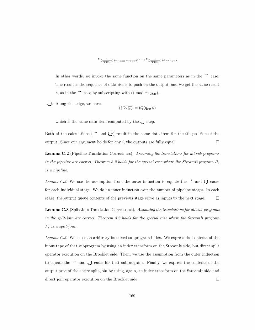
z(〈 ixPUSH

〉+xPEEK−xPOP), . . . , z(〈 ixPUSH

〉+1−xPOP)

In other words, we invoke the same function on the same parameters as in the case.

The result is the sequence of data items to push on the output, and we get the same result

zi as in the case by subscripting with (i mod xPUSH).

: Along this edge, we have:([[Ob ]]ob)i = (Q(qout)i)

which is the same data item computed by the step.

Both of the calculations ( and ) result in the same data item for the ith position of the

output. Since our argument holds for any i, the outputs are fully equal.

Lemma C.2 (Pipeline Translation Correctness). Assuming the translations for all sub-programs

in the pipeline are correct, Theorem 3.2 holds for the special case where the StreamIt program Ps

is a pipeline.

Lemma C.2. We use the assumption from the outer induction to equate the and cases

for each individual stage. We do an inner induction over the number of pipeline stages. In each

stage, the output queue contents of the previous stage serve as inputs to the next stage.

Lemma C.3 (Split-Join Translation Correctness). Assuming the translations for all sub-programs

in the split-join are correct, Theorem 3.2 holds for the special case where the StreamIt program

Ps is a split-join.

Lemma C.3. We chose an arbitrary but fixed subprogram index. We express the contents of the

input tape of that subprogram by using an index transform on the StreamIt side, but direct split

operator execution on the Brooklet side. Then, we use the assumption from the outer induction

to equate the and cases for that subprogram. Finally, we express the contents of the

output tape of the entire split-join by using, again, an index transform on the StreamIt side and

direct join operator execution on the Brooklet side.

160

D

Data Parallelism Optimization

Correctness

This section sketches the proof for Theorem 3.3 in Section 3.4.1.

Let bin and bout be the sequences of all data items that ever appear on queues qin and qout ,

respectively. Because every Brooklet queue is defined only once and because op is stateless, bin

fully determines bout . Since f commutes, bout has the same contents in both Pb and P ′b. Since

round-robin split-joins preserve order, bout has the same order in both Pb and P ′b.

161

E

Fusion Optimization Correctness

This section sketches the proof for Theorem 3.4 in Section 3.4.2.

Let bin and bout be the sequences of all data items that ever appear on queues qin and qout ,

respectively. Because every queue is defined only once and because only op1 and op2 write v1

and v2, bin fully determines bout . We can show that bout is the same for both Pb and P ′b by

induction over bin .

162

F

Selection Hoisting Optimization

Correctness

This section sketches the proof for Theorem 3.5 in Section 3.4.3.

The input data on q fully determines the output data on qout , because the operators are

stateless. We can show by induction over the input data that the output data is the same for

both Pb and P ′b. The proof relies on the fact that f1 only reads data forwarded unmodified by

f2 and vice versa.

163