Returns to Education in Four Transition Countries: Quantile Regression Approachftp.iza.org/dp5210.pdf · Returns to Education in Four Transition Countries: Quantile Regression Approach

DI

SC

US

SI

ON

P

AP

ER

S

ER

IE

S

Forschungsinstitut zur Zukunft der ArbeitInstitute for the Study of Labor

Returns to Education in Four Transition Countries: Quantile Regression Approach

IZA DP No. 5210

September 2010

Anita StanevaG. Reza ArabsheibaniPhilip Murphy

Returns to Education in Four Transition

Countries: Quantile Regression Approach

Anita Staneva Swansea University

G. Reza Arabsheibani

Swansea University and IZA

Philip Murphy Swansea University

Discussion Paper No. 5210 September 2010

IZA

P.O. Box 7240 53072 Bonn

Germany

Phone: +49-228-3894-0 Fax: +49-228-3894-180

E-mail: [email protected]

Any opinions expressed here are those of the author(s) and not those of IZA. Research published in this series may include views on policy, but the institute itself takes no institutional policy positions. The Institute for the Study of Labor (IZA) in Bonn is a local and virtual international research center and a place of communication between science, politics and business. IZA is an independent nonprofit organization supported by Deutsche Post Foundation. The center is associated with the University of Bonn and offers a stimulating research environment through its international network, workshops and conferences, data service, project support, research visits and doctoral program. IZA engages in (i) original and internationally competitive research in all fields of labor economics, (ii) development of policy concepts, and (iii) dissemination of research results and concepts to the interested public. IZA Discussion Papers often represent preliminary work and are circulated to encourage discussion. Citation of such a paper should account for its provisional character. A revised version may be available directly from the author.

IZA Discussion Paper No. 5210 September 2010

ABSTRACT

Returns to Education in Four Transition Countries: Quantile Regression Approach

This paper uses quantile regression techniques to analyze heterogeneous patterns of return to education across the conditional wage distribution in four transition countries. We correct for sample selection bias using a procedure suggested by Buchinsky (2001), which is based on a Newey (1991, 2009) power series expansion. We also examine the empirical implications of allowing for the endogeneity of schooling, using the control function approach proposed by Lee (2007). Using household data from Bulgaria, Russia, Kazakhstan and Serbia in 2003, we show that the return to education is heterogeneous across the earnings distribution. It is also found that accounting for the endogeneity of schooling leads to a higher rate of return to education. JEL Classification: C14, I2, J24 Keywords: rate of return to education, endogeneity, sample selection, quantile regression Corresponding author: G. Reza Arabsheibani School of Business and Economics Swansea University Richard Price Building Singleton Park Swansea, SA2 8PP United Kingdom E-mail: [email protected]

2

1. Introduction

Understanding the heterogeneous pattern of return to education across the

conditional earnings distribution requires recognition of the affect that „ability‟ and/or

„endogeneity‟ bias can have on the estimated returns. Human capital theory implicitly

recognises that the return to education may be heterogeneous. Inter alia educational

returns can vary across schooling levels and even across individuals with the same

schooling level. Typically mean based regression models, like Ordinary Least Squares

(OLS), fail to recognise this and so the estimated return from these models is unlikely

to be an appropriate representation of the data. To place this idea into context we can

envisage a process in which individuals are likely to differ with respect to not only the

perceived benefits of education, but also the cost of education and the choices

subsequently made in the labour market. In such circumstances the return to education

is unlikely to be a single parameter; instead it is likely to vary systematically

according to differences in individual‟s unmeasured characteristics, which in turn

determine where in the overall earnings distribution an individual is placed. More

generally any uncontrolled effect that is systematically correlated with an individual‟s

position in the earnings distribution and which is also correlated with education

attainment implies that the return to education is likely to vary across the earnings

distribution. Accounting for this heterogeneity, therefore, requires an estimation

strategy that allows the return to education to differ at different points in the earnings

distribution.

An estimation procedure that allows the return to education to differ at

different points in the earnings distribution is the quantile regression (QR) model, and

in this paper we use the QR model to address three important empirical questions.

First, we examine the extent to which the return to education varies across the

3

conditional earning distribution in four transition countries (Bulgaria, Russia,

Kazakhstan and Serbia) in 2003. Second, we consider the impact sample selection

bias has on the returns to education in the QR framework using Buchinsky‟s (1998,

2001) power series estimator1. Third, we investigate the empirical implications of

allowing schooling to be endogenous (individual self-selection in the education

process) in a QR context, using a control function approach proposed by Lee (2007).

The paper is organized as follows. In section 2, we briefly describe the

education system in the selected transition countries. In section 3, the theory of

quantile regression and endogeneity correction is presented, along with a brief

discussion of Buchinsky‟s method for correcting for selectivity bias. In section 4, we

comment on the data used in the estimation. Finally, sections 5 and 6 discuss the main

results and conclusions.

2. Education in transition to a Market Economy

The education system and educational attainment is an essential feature of the

transition process in Central and Eastern Europe and the Former Soviet Union.

Typically the stock of human capital inherited by these countries from the socialist

period was high by the standards of other countries at similar stages of their economic

development. However, while the countries used in this study share a number of

common influences, the paths of economic development followed by them differ in

number of important respects, which makes for an interesting comparison of their

earnings-education profiles.

There is a common perception in the literature to view Bulgaria and Serbia as

Balkan countries in which the economic reforms following the break-up of the Soviet

Union have progressed more slowly compared to the more advanced reform countries

located in Central Europe. However, even within this simple classification interesting

4

differences are still evident. For example, there are important differences between

Serbia and Bulgaria both with respect to the speed of educational reforms and the

impact these then had on labour market outcomes (Arandarenko, Kotzeva and Pauna

2006).

Bulgaria

Education in Bulgaria, although fundamentally national in character, has

significant foreign influences. The Soviet influence was most evident during the

period of the national revival in the nineteenth century and reflected the ideas of

Slavophilism and pan-Orthodoxy. Education in Bulgaria is compulsory between the

ages of 7 to 16. Prior to higher education the schooling system in Bulgaria consists of

12 school grades, organized in two major levels of study: basic and secondary. Basic

education (grades one to eight) is divided into two sub-levels: elementary (grades one

to four) and pre-secondary (grades five through eight). Secondary education normally

encompasses grades eight to twelve and there are two major types of secondary

schools: secondary comprehensive, usually called gymnasia (high school) and

secondary vocational, most often referred to as tehnikum (vocational school).

Russia

Russia is an interesting case with transition from a planned economy to a

market based economy that featured both over-education and over-employment,. The

stages of compulsory schooling in Russia are: primary education for ages 6-7 to 9-10

inclusive; senior school for ages 10-11 to 12-13 inclusive, and senior school for ages

13-14 to 14-15 inclusive. If a secondary school pupil wishes to go on to higher

education, he or she must stay at school for another two years. Primary and secondary

schooling together account for 11 years of study, split into elementary (grades 1-4),

middle (grades 5-9) and senior (grades 10-11) classes.

5

Kazakhstan

As part of the Soviet Union, Kazakhstan achieved remarkably high attainment

rates in education. During the Communist era education was a key priority and free

compulsory schools were a feature of the Kazakhstan education system. The

education system in Kazakhstan was highly responsive to the needs of a totalitarian

regime and as a result was generously funded. Following independence, however,

there was a dramatic drop in expenditure on education, which resulted in the closure

of many facilities including pre-school nurseries that were highly dependent on state

funding (Arabsheibani and Mussurov 2007).

Education in Kazakhstan starts at age 6 with pre-school preparation. Primary

level starts at the age of 7 and continues for 3 years, with basic primary level

extending to an additional 5 years at the basic secondary level. After successfully

completing basic secondary level students proceed to general secondary (2 years) or

to either vocational training (2-4 years) or Tehnikums (professional college).

University level studies are divided between undergraduate and postgraduate levels

with university degrees typically awarded after five years of study.

Serbia

Following the break-up of Yugoslavia and the problems it faced thereafter

Serbia is today one of the poorest countries in Europe. The progress towards a stable

democratic system in Serbia has been slow but amidst all of its problems Serbia has

begun to rebuild and reform its education system. The link between poverty and

education in Serbia is very strong, with 71% of the poor being without education or

with only primary school education2. According to the last Census of population in

2002, 3.45% of the population were illiterate and almost one million had not even

completed primary schooling3. The education system in Serbia includes preschool,

6

primary, secondary, higher, and university education. Preschool covers children from

6 to 7 years old. Primary education lasts eight years, and it is the only compulsory part

of education system in Serbia. Secondary education follows primary education and

while it is not compulsory it is free for all. Secondary schools are divided into

gymnasiums and vocational schools, each of which lasts 3 or 4 years. Considerable

reforms in the field of higher education have taken place in Serbia since it became a

signature of the Bologna declaration in September 2003.

3. Econometric methodology

Quantile regression approach

Our distributional approach is based on the use of Quantile Regression (QR)

(Koenker and Bassett 1978), which provides estimates of the effect of education on

earnings at different points of the earnings distribution. Estimating the effect of

education at conditional quantiles, therefore, allows for heterogeneity in the returns to

education. Just as least square models the conditional mean of the dependent variable

Y relative to the covariates X used in the analysis, quantile egressions give estimates

of the effect of covariates at different percentiles of the conditional distribution4.

In a wage equation setting, the quantile regression model can be written as:

iii uXY ln

with iii XXYQ )|(ln

(1)

where )|(ln ii XYQ denotes the conditional quantile of iYln , conditional on the

regressor vector iX .

Estimates at different quantiles can be interpreted as showing the response of

the dependent variable to the regressors at different points in the conditional wage

distribution. The relative positioning of workers in the conditional wage distribution,

therefore, can be related to systematic differences in unobservables, which generically

7

may be referred to as „ability‟ and include a diverse range of attributes like

motivation, labour market connections, family human capital, school quality, etc

(Arias, Hallock and Escudero 2001).

Sample selection in quantile regression framework

There is an additional complication that is not accounted for in the description

of the QR given above, namely pre-selection into employment. Specifically working

women and men may not be a randomly selected sample from the overall population,

which can lead to biased estimates of the earnings equation5. Methods for correcting

selectivity bias in quantile regression models have only recently been developed. The

bivariate normality assumption typically made in the OLS model between the error

terms in the earnings and participation equation will not necessarily hold in the

quantile regression case. Buchinsky (1998) suggests an approach using the non-

parametric procedure of Newey (1991) to deal with this problem, and in this

application the presence of children in the household is used as the identifying

restriction in the participation equation. The estimation procedure followed can be

briefly described as follows. First, an estimate of the latent index determining labour

market participation is found from a standard Probit model. Estimates of the latent

index from this model are then used as an argument in a power series expansion,

which is designed to approximate the unknown quantile functions of the truncated

bivariate distribution of the error terms in the wage and participation equations.

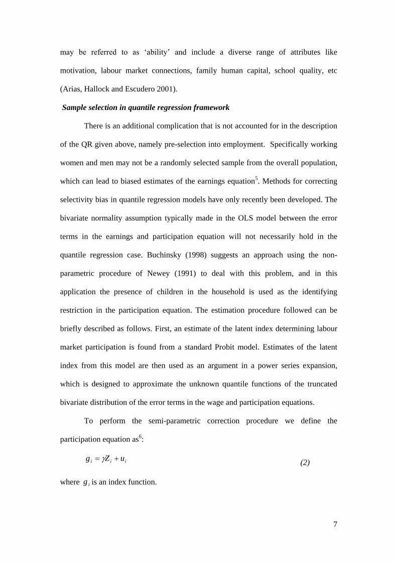
To perform the semi-parametric correction procedure we define the

participation equation as6:

iii uZg (2)

where ig is an index function.

8

To get unbiased estimates of for the male and female respondents it is

necessary to introduce an extra term:

iiii ghXY )(ln (3)

where:

)0,()( iiii gZQuantgh (4)

The term )( igh includes information about the unobservables that affect individual

labour force participation decisions. The estimated probability function provides the

location for the index )ˆ(ˆiZg and the values of iZg ̂ˆ are used to expand )( igh in

a power series by approximating:

1

1)ˆ()(ˆ

k

i

k

k

k

i gZg (5)

where k is the number of terms in the approximating series, which is allowed to grow

with the sample size. In the results reported experimentation with different power

series indicated that a second order power series was sufficient in each case7.

Endogeneity in the quantile regression model

In many empirical regression models, it is common to have a regressor that is

endogeneous8. If the return to schooling is endogenous estimates of the returns to

education from a standard QR model may be misleading. To control for endogeneity

bias in a quantile regression framework, we adopt the control function approach

proposed by Lee (2007). As an alternative to existing methods in the literature, Lee‟s

methodology extends the control function approach to the structural quantile

regression model semi-parametrically. He shows that under suitable conditions, the

estimator obtained from the control function approach is consistent and

asymptotically normally distributed.

9

Formally Lee (2007) considers the following model, which is a semi-

parametric quantile regression version of Newey, Powell and Vella (1999):

UZXY )(')( 1 (6)

VZX )(')( (7)

where Y is the dependent variable, X is real-valued continuously distributed

endogenous explanatory variable, ),( 21 ZZZ is a )1( zd vector of exogenous

explanatory variables, U and V are real-valued unobserved random variables,

)( and )( are unknown structural parameter of interest, )( is an unknown

parameter, )](),([)( 21 vector is a )1( zd vector of unknown parameters

for some and such that 10 and 10 . For identification it is assumed

that there is at least one component of Z that is not included in 1Z , and that there is at

least one non-zero coefficient for the excluded components of Z. That is,

zz dd 1 and 0)(2 , where 1zd is the dimension of 1Z .

In our return to education estimates, the reduced- form schooling residuals V

are interpreted as „individual ability‟ and therefore U is not assumed to be

independent of V. The approach corrects for endogeneity by adding residual power

series estimates as additional explanatory variables and is interpreted as a variant of

control function approach9(e.g., Newey, Powell and Vella 1999; Blundell and Powell

2003b).

Following the method proposed by Trostel, Walker and Woolley (2002), we

use spouse‟s education as an instrument. The instrument should be correlated with the

partner‟s education while uncorrelated with the error term in the earnings equation.

Assortative mating can be invoked to ensure there is a correlation between partners

education, either as a result of household specialisation or as a result of partners

sharing common interests and that that lead to them having similar levels of schooling

10

(Pencavel 1998). As Trostel et al. (2002) point out, however, assuming no association

between „spouse‟s‟ education and the error term in the partners earnings equation is

potentially more problematic, particularly if the level of schooling of both partners are

complements in the production of household income. Because Trostel et al had more

than one potential instrument to use in their analysis they were able to undertake a

Sargan instrument validity test to provide support for their empirical approach.

Unfortunately in most of the countries dealt with in this paper we only have one

identifying instrument and are, therefore, unable to undertake a similar test. However,

in the case of Kazakhastan we have access to the same instruments used in the Trostel

et al paper (spouses and mothers education). In this case a Sargan instrument validity

test was passed for both male and female samples, which we feel provides some

support for the approach adopted here.

4. The Data

We use data from the Bulgarian Multi-Topic Household Survey (2003), the

Russian NOBUS Survey (2003), the Kazakhstan Household Budget Survey (2003)

and Serbian Living Standard Measurement Survey (2003) in the analysis reported

below.

The Bulgarian Multi-Topic Household Survey, which was carried out in

October and November 2003, includes information on income, expenditures,

demographic and labour market characteristics for a representative sample of 3,023

Bulgarian households. The subset of the data used in the estimation consists of a

sample of 1,296 men and 1,186 women. Table 1 reports summary statistic for the

sample of working men and women. The descriptive statistics indicate that average

log hourly wage rate for men in Bulgaria is higher for men than it is for women.

Moreover, women have more years of schooling than men, reflecting the fact that

11

women that work in Bulgaria are more likely to have participated in higher education

than men. Thus, while 62% of employed men and 53% of employed women in

Bulgaria have secondary schooling, 26% of working women have a university degree

compare to only 17 % of men.

The Russian NOBUS dataset provides detailed information on household

consumption and income; together with information on household demographics,

labour market participation, access to health, education and social programs, and

subjective perceptions of household welfare. Summary statistics for the Russian

working sample are presented in Table 2, and consists of 21,874 men and 24,318

women. There are considerable differences in the characteristics of men and women

with respect to both educational qualifications and occupational status. The data

indicates that women earn less than men, with a raw gender wage gap of about 26%.

We can see that a higher proportion of women than men have completed a university

degrees (24% and 18% respectively), while a significantly higher proportion of

working men are married (76%) compared to women who are much more likely to

have been divorced. This suggests that the labour market participation of women in

Russia is significantly affected by their marital status and by the need of divorced

women to work following the break-up of their marriages. Not surprisingly, women‟s

employment is more concentrated than men‟s in the public sector (69% of female

employment is in the public sector compared to only 60% of male employment), and

as a result women are less represented in the private sector where both job

opportunities and employment flexibility are less likely to as attractive to workers.

The Kazakhstan data (KHBS) was collected by the Kazakhstan Agency of

Statistics with technical assistance from the World Bank. The survey covers

household income and employment, health and education attainment. The sample is

12

randomly selected and based on a register of household dwelling in Kazakhstan. After

excluding students, children who are less than 16 years of age, and pensioners the

sample consist of 16,375 individuals, of whom 7,868 are male and 8,507 are female.

Table 3 reports the main descriptive statistics. The Kazakhstan sample does not

provide a direct measure of the years of individual schooling, instead respondents are

asked about their highest level of education attainment. The schooling variable used

in the analysis, therefore, is constructed in the following way: if no qualification or

nursery education is indicated S=1, if primary S=3, if general secondary S=8, if high

school S=10, if vocational technical school S=10, if college S=12, if degree S=15 and

if postgraduate S=20 (see Arabsheibani and Mussurov 2006). The dependent variable

in the analysis is earnings reported after taxes. Unfortunately, unlike the other surveys

used in this paper, the Kazakhstan survey did not ask about the number of hours

worked by individuals, as a result monthly income is taken as the measure of earnings

for Kazakhstan. Specifically, the dependent variable used in the analysis is the log of

monthly earnings received from the main job, and excludes earnings from secondary

jobs, or from agricultural production, and non-monetary benefits.

The descriptive statistics for Kazakhstan reported in Table 3 show that as in

the other transition countries women earn less than men. Women are also more likely

to be employed in the public sector and have more years of schooling. The percentage

of working women in Kazakhstan that have a university degree is 24% compared to

only 17% for men.

Finally to estimate the return to education in Serbia, we use Serbian Living

Standard Measurement Survey (2003). The Labour Market module in this survey is

similar to the Labour Force Survey (LFS), but with additional questions to capture

informal sector activities that provide more detailed information on earnings. The

13

sample used in the analysis consists of 2,548 households of which 2,450 individuals

have information on hourly earnings. Table 4 reports the main descriptive statistics.

The average log hourly wage rate is higher for men than for women, and 11.4% of

employed women in Serbia have obtained a university degree compared to only 7.7%

of men.

5. Empirical Results

The QR models estimated in this paper are based on an augmented Mincer (1974)

earnings equation, with the natural logarithm of earnings regressed on an individual‟s

completed years of schooling and potential labour market experience (and its square).

Additional controls for marital status, job-tenure, region of work, ethnicity, public

sector employment, health, and managerial responsibilities are also included in the

analysis. The Russian specifications is also supplemented with series of variables that

capturing part-time employment and wage arrears effects10

.

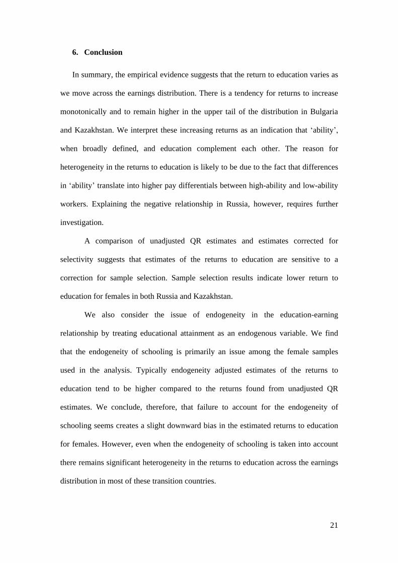
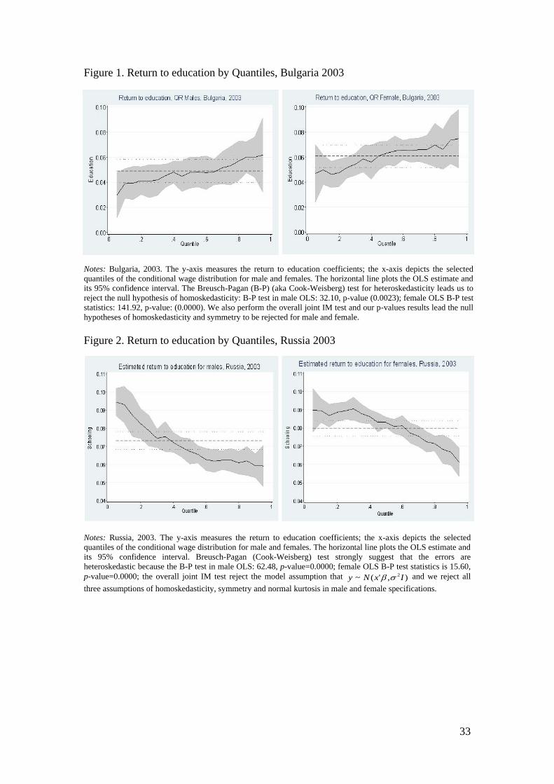
Bulgaria

We first estimate the Bulgarian earning function assuming schooling is

exogenous. Tables 5 and 6 report the QR estimates for five values of (10th

, 25th

,

50th

, 75th

and 90th

percentiles) for Bulgarian males and females respectively. The

estimated returns to schooling are also plotted for each percentile in Figure 1, along

with the 95 % confidence interval for each point estimate. Superimposed on the plot,

in Figure 1, is a dashed line representing the OLS estimate of the effect of education

on hourly earnings. Each side of the OLS estimate is a dotted line which shows the

associated 95% confidence interval of the estimate.

Figure 1 about here

Table 5 about here

Table 6 about here

14

The effect of education on wages is positive and statistically different from

zero at each of the reported percentiles. This indicates hourly earnings in Bulgaria

increase with education throughout the conditional wage distribution. Moreover, the

horizontal line in Figure 1, which plots the OLS estimate and its 95% confidence

interval, indicates that the estimated mean return to schooling is not representative of

the effect education has on earnings at all points in the earnings distribution. Instead

the return to schooling is higher at higher points in the earnings distribution. For

instance, the return to schooling for males in Bulgaria increases from 3.9% to 6.0%

between the 10th

and 90th

percentile and from 4.9% to 7.4% for females (See Table 5

and Table 6)11

. In this case, therefore, schooling has a positive impact upon wage

inequality in Bulgaria. Arias, Hallock and Escudero (2001) have interpreted a positive

ability-returns relationship as evidence that education and ability are complements in

the human capital generation process, which if true suggests that more able

individuals in Bulgaria benefit most from educational investment. However, there

might be other explanations for this pattern. Because personal abilities and skills

(cognitive and non-cognitive) are unobserved by economists, it is difficult to isolate

the effect that drives the heterogeneous pattern of returns to education across the wage

distribution. For example, workers with identical education do not necessarily have to

have the same level of productivity because of the influence of unobserved variables

that are systematically correlated with both measured education and an individual‟s

place in the earnings distribution.

More generally the Bulgarian results reported here are consistent with

previous estimates reported in the literature. Martins and Pereira (2004) and Flabbi,

Paternostro and Tiongson (2008), for example, both report higher returns to education

at the top end of the conditional wage distribution.

15

Following Vella (1998), we estimate the latent index )ˆ(ˆiZg that determines

male and female labour market participation parametrically using a probit model. A

range of familiar variables are used as covariates in the participation equation,

including the presence of dependent children in the household which is used to

identify the participation on the assumption that this variable is exogenous12

. An

estimate of the latent index from the participation equation is then used in a power

series to obtain estimates of the selectivity adjusted QR model. Selection corrected

estimates for Bulgaria indicate that the power series correction terms included in the

QR analysis were not significant for either males or females workers. We can

conclude, therefore, that sample selection effects are not an issue for the estimation of

male and female earnings equations in Bulgaria (Table 5 and Table 6).

We adjust for endogeneity bias by using the Lee‟s (2007) control function

approach. A fifth order polynomial of the reduced form residuals is used in the

analysis to estimate the return to schooling at different values of 13. Spouse‟s

education is used as an instrument, and there is a significant and positive relationship

between this variable and the partner‟s level of schooling14

. A Durbin-Hausman Wu

test (DWH) (Davidson and McKinnon 1993) is used to test the hypothesis of

endogeneity of schooling15

. The results are not sensitive to the choice of the order of

the residual polynomial used in the analysis. In the male specification (Table 5) there

is no statistical difference between unadjusted QR return to education and the return

to education adjusted for endogeneity using the control function approach. This

finding is supported by the insignificance of the power terms included in the male

equation and by the DWH test that fails to reject the null that schooling is exogenous.

We can conclude, therefore, that male schooling is exogenous and accept the

unadjusted QR estimates being consistent estimates of the returns to schooling. On the

16

other hand, the DWH test undertaken on the female earnings equation leads to a

strong rejection of the null hypothesis of exogeneity of schooling and the endogeneity

adjusted QR results for females are quite different from the unadjusted QR results. In

particular the endogeneity adjusted female QR results show a much more

heterogeneous pattern of return to education as we move across the earnings

distribution (Table 6). Specifically correcting for the endogeneity of schooling

increases the return to schooling at each point in the earnings distribution for females

in Bulgaria, but the effect is much more pronounced at the top end of the distribution.

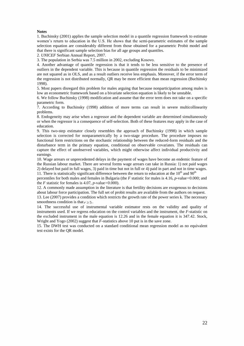
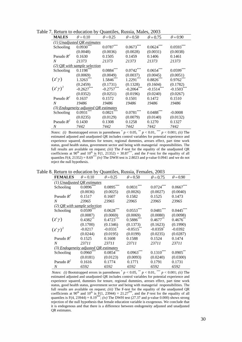
Russia

Figure 2 shows the estimated returns to education for Russian males and

females at different percentiles, assuming schooling to be exogenous. Both male and

female results show that return to schooling is higher in the lower part of the earnings

distribution than at the top end of the distribution. For instance, the returns to

education for males fall from 9.3% to 5.9% between the 10th

and 90th

quantile (Table

7) and for females the equivalent fall is from 8.9% to 6.6% (Table 8). Moreover these

differences are significant as an F-test decisively rejects the equality of the estimates

at the 10th

and 90th

percentiles for both male and female workers in Russia.

Figure 2 about here

Table 7 about here

Table 8 about here

Mwabu and Schultz (1996) and Arias, Hallock and Escudero (2001) interpret

a negative ability-returns relationship as evidence of education and ability being

substitutes, which implies that maximising the returns to education may require

increasing educational opportunities for less able individuals in Russia. Flabbi

Paternostro and Tiongson (2008) also find evidence for a higher return to education in

17

the lower part of the earnings distribution in Russian in the early (1991-1996) and late

transition (1997-2002) periods. Similarly Gorodnichenko and Sabirianova (2005) find

that the university wage premium in Russia is higher in the lower part of the earnings

distribution than in top part of the earnings distribution.

There are, however, a number of alternative explanations for this pattern. First,

a demand-side effect could drive down the return to education at different points in

earnings distribution because of an oversupply of well-educated workers in the

economy (the supply effect dominates the demand effect at higher points in the

earnings distribution). Second, a negative relationship between „ability‟ and the

return to schooling could also reflect differences in the educational attainment of the

labour force (Herrnstein and Murray 1994). Similarly, lower returns to education at

the higher end of the earnings distribution suggests there are factors leading to high-

paying employment that act independently of education-generating human capital

process. It is also possible to interpret the results in terms of a “state” or “foreign”

ownership effect. State ownership is much more relevant to the lower tail of the wage

distribution and relatively low paid workers earn more in stated owned firms.

However, this state ownership effect tends to die away as there is movement up

through the earnings distribution (Machado and Mata 2001).

A comparison of unadjusted QR estimates and those corrected for sample

selectivity suggests that the return to education in Russia is sensitive to this correction

(Tables 7 and 8). The selection corrected male education return is slightly higher

compared to that when selection is ignored and the difference tends to be higher at the

bottom of the distribution than at the top. By way of contrast the female selectivity

corrected estimates indicate that the return to schooling is lower in the unadjusted QR

results at all points in the earnings distribution.

18

Endogeneity adjusted QR estimates for males reported in Table 7 indicate that

apart from the 90th

percentile, where the return to education is insignificant and

negative, the effect of correcting for the endogeneity of schooling has little affect on

the estimates return to schooling at other percentile levels. This finding is supported to

some extent by the DWH test, which fails to reject the null that schooling is

exogenous. However, endogeneity adjusted returns to schooling are quite different for

females in Russia, where the effect of adjusting for endogeneity of schooling typically

increases the adjusted returns to education. Moreover, this effect tends to be more

pronounced in the top end of the distribution than in the bottom end of the

distribution.

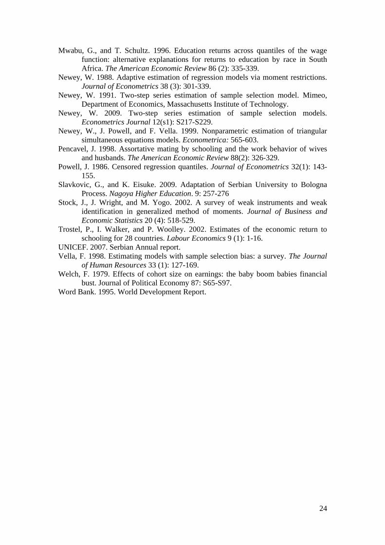
Kazakhstan

The Kazakhstan QR estimates are presented in Tables 9 and 10. The returns to

education at different percentiles are also shown in Figure 3. OLS returns differ

significantly from QR returns and as in other countries reported in this paper the QR

estimates are all positive and significantly different from zero. Tables 9 and 10

indicate that the estimated return to education in Kazakhstan for both males and

females are lowest in the bottom end of the earnings distribution and tend to increase

as we move up through the distribution. Interestingly the returns to education for

females tend to increase more rapidly than the corresponding return for men,

suggesting that inequality is more pronounced for females than men in terms

educational returns. At the highest percentile (90th

) the return to schooling is 6.4%

for females and 4.8% for males, while the equivalent comparison at the 10th

percentile

is a return of 1.2% for females and 2.4% for males. A test of whether the estimated

returns to education differ across each of these percentile levels indicates that there is

significant difference in the returns for both male and female workers in Kazakhstan.

19

Evidence of sample selectivity effects for males in Kazakhstan is provided by

the significance of the second order term in the series approximation. Correcting for

selection has a dramatic effect on the returns to schooling for males in this sample,

reducing the return to a level which is not significantly different from zero at all

percentiles (Table 9). If true this finding would suggest that for males in Kazakhstan

education is important for determining participating in the labour force but thereafter

has little effect on the earnings of individuals. The coefficients on both selection terms

in the female earnings equation are significant at all percentile levels. However, while

correcting for participation into work results in reduction in the female return to

education at most percentiles, the difference between the adjusted and unadjusted QR

estimates is not statistically significant.

Figure 3 about here

Table 9 about here

Table 10 about here

An examination of the results in Tables 9 and 10 suggests that the effects of

adjusting for the endogeneity of schooling is most marked at the top end of the

earnings distribution for both male and female workers in Kazakhstan. Endogeneity

corrected returns to education are typically higher in the top end of the distribution

than those reported for the unadjusted results. The same pattern is also evident for

males and females at the 10th

percentile, but at intervening points in the earnings

distribution the difference between the unadjusted QR estimates and those corrected

for endogeneity are much less marked.

Serbia

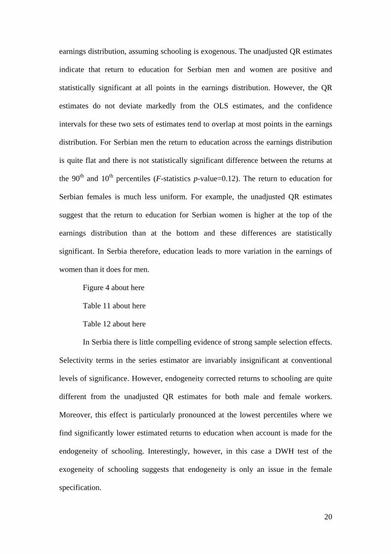
The Serbian QR results are reported in Tables 11 and 12. Figure 4 also plots

the unadjusted QR estimates of the return to education across different points in the

20

earnings distribution, assuming schooling is exogenous. The unadjusted QR estimates

indicate that return to education for Serbian men and women are positive and

statistically significant at all points in the earnings distribution. However, the QR

estimates do not deviate markedly from the OLS estimates, and the confidence

intervals for these two sets of estimates tend to overlap at most points in the earnings

distribution. For Serbian men the return to education across the earnings distribution

is quite flat and there is not statistically significant difference between the returns at

the 90th

and 10th

percentiles (F-statistics p-value=0.12). The return to education for

Serbian females is much less uniform. For example, the unadjusted QR estimates

suggest that the return to education for Serbian women is higher at the top of the

earnings distribution than at the bottom and these differences are statistically

significant. In Serbia therefore, education leads to more variation in the earnings of

women than it does for men.

Figure 4 about here

Table 11 about here

Table 12 about here

In Serbia there is little compelling evidence of strong sample selection effects.

Selectivity terms in the series estimator are invariably insignificant at conventional

levels of significance. However, endogeneity corrected returns to schooling are quite

different from the unadjusted QR estimates for both male and female workers.

Moreover, this effect is particularly pronounced at the lowest percentiles where we

find significantly lower estimated returns to education when account is made for the

endogeneity of schooling. Interestingly, however, in this case a DWH test of the

exogeneity of schooling suggests that endogeneity is only an issue in the female

specification.

21

6. Conclusion

In summary, the empirical evidence suggests that the return to education varies as

we move across the earnings distribution. There is a tendency for returns to increase

monotonically and to remain higher in the upper tail of the distribution in Bulgaria

and Kazakhstan. We interpret these increasing returns as an indication that „ability‟,

when broadly defined, and education complement each other. The reason for

heterogeneity in the returns to education is likely to be due to the fact that differences

in „ability‟ translate into higher pay differentials between high-ability and low-ability

workers. Explaining the negative relationship in Russia, however, requires further

investigation.

A comparison of unadjusted QR estimates and estimates corrected for

selectivity suggests that estimates of the returns to education are sensitive to a

correction for sample selection. Sample selection results indicate lower return to

education for females in both Russia and Kazakhstan.

We also consider the issue of endogeneity in the education-earning

relationship by treating educational attainment as an endogenous variable. We find

that the endogeneity of schooling is primarily an issue among the female samples

used in the analysis. Typically endogeneity adjusted estimates of the returns to

education tend to be higher compared to the returns found from unadjusted QR

estimates. We conclude, therefore, that failure to account for the endogeneity of

schooling seems creates a slight downward bias in the estimated returns to education

for females. However, even when the endogeneity of schooling is taken into account

there remains significant heterogeneity in the returns to education across the earnings

distribution in most of these transition countries.

22

Notes

1. Buchinsky (2001) applies the sample selection model in a quantile regression framework to estimate

women‟s return to education in the U.S. He shows that the semi-parametric estimates of the sample

selection equation are considerably different from those obtained for a parametric Probit model and

that there is significant sample selection bias for all age groups and quantiles.

2. UNICEF Serbian Annual Report, 2007.

3. The population in Serbia was 7.5 million in 2002, excluding Kosovo.

4. Another advantage of quantile regression is that it tends to be less sensitive to the presence of

outliers in the dependent variable. This is because in quantile regression the residuals to be minimized

are not squared as in OLS, and as a result outliers receive less emphasis. Moreover, if the error term of

the regression is not distributed normally, QR may be more efficient than mean regression (Buchinsky

1998).

5. Most papers disregard this problem for males arguing that because nonparticipation among males is

low an econometric framework based on a bivariate selection equation is likely to be unstable.

6. We follow Buchinsky (1998) modification and assume that the error term does not take on a specific

parametric form.

7. According to Buchinsky (1998) addition of more terms can result in severe multicollinearity

problems.

8. Endogeneity may arise when a regressor and the dependent variable are determined simultaneously

or when the regressor is a consequence of self-selection. Both of these features may apply in the case of

education.

9. This two-step estimator closely resembles the approach of Buchinsky (1998) in which sample

selection is corrected for nonparametrically by a two-stage procedure. The procedure imposes no

functional form restrictions on the stochastic relationship between the reduced-form residuals and the

disturbance term in the primary equation, conditional on observable covariates. The residuals can

capture the effect of unobserved variables, which might otherwise affect individual productivity and

earnings.

10. Wage arrears or unprecedented delays in the payment of wages have become an endemic feature of

the Russian labour market. There are several forms wage arrears can take in Russia: 1) not paid wages

2) delayed but paid in full wages, 3) paid in time but not in full or 4) paid in part and not in time wages.

11. There is statistically significant difference between the return to education at the 10th and 90th

percentiles for both males and females in Bulgaria (the F statistic for males is 4.16, p-value=0.000; and

the F statistic for females is 4.07, p-value=0.000).

12. A commonly made assumption in the literature is that fertility decisions are exogenous to decisions

about labour force participation. The full set of probit results are available from the authors on request.

13. Lee (2007) provides a condition which restricts the growth rate of the power series k. The necessary

smoothness condition is that 5r .

14. The successful use of instrumental variable estimator rests on the validity and quality of

instruments used. If we regress education on the control variables and the instrument, the F-statistic on

the excluded instrument in the male equation is 12.26 and in the female equation it is 347.42. Stock,

Wright and Yogo (2002) suggest that F-statistics above 10 put is in the save zone.

15. The DWH test was conducted on a standard conditional mean regression model as no equivalent

test exists for the QR model.

23

References

Arabsheibani, G. Reza, and A. Mussurov. 2007. Returns to schooling in Kazakhstan:

OLS and instrumental variables approach. Economics of Transition 15(2):

341-364.

Arandarenko, M., M. Kotzeva, and B. Pauna. 2006. Valuing Human capital in Balkan

Transition countries.

Arias, O., K. Hallock, and W. Sosa-Escudero. 2001. Individual heterogeneity in the

returns to schooling: instrumental variables quantile regression using twins

data. Empirical Economics 26(1): 7-40.

Blundell, R., and J. Powell. 2003b. Endogeneity in nonparametric and semiparametric

regression models. Review of Economic Studies, forthcoming

Buchinsky, M. 1994. Changes in the US wage structure 1963-1987: Application of

quantile regression. Econometrica: 405-458.

Buchinsky, M. 1995. Estimating the asymptotic covariance matrix for quantile

regression models. A Monte Carlo study. Journal of Econometrics 68(2): 303-

338.

Buchinsky, M. 1998. The dynamics of changes in the female wage distribution in the

USA: a quantile regression approach. Journal of Applied Econometrics 13(1):

1-30.

Buchinsky, M. 2001. Quantile regression with sample selection: Estimating women's

return to education in the US. Empirical Economics 26(1): 87-113.

Davidson, R., and J. MacKinnon. 1993. Estimation and inference in econometrics.

New York : Oxford University Press.

Denny, K., and V. O'Sullivan. 2007. Can education compensate for low ability?

Evidence from British data. Applied Economics Letters 14 (7-9): 657-660.

Eren, O. 2009. Ability, Schooling Inputs and Earnings: Evidence from the NELS.

Canadian Economic Association Meetings at University of British Columbia

June, 2008.

Flabbi, L., S. Paternostro, and E. Tiongson. 2008. Returns to education in the

economic transition: A systematic assessment using comparable data.

Economics of Education Review 27(6): 724-740.

Gorodnichenko, Y., and K. Sabirianova. 2005. Returns to schooling in Russia and

Ukraine: A semiparametric approach to cross-country comparative analysis.

Journal of Comparative Economics 33(2): 324-350.

Herrnstein, R., and C. Murray. 1994. The bell curve: Intelligence and class structure

in American life. New York.

Koenker, R., and G. Bassett. 1978. Regression quantiles. Econometrica 46(1): 33-50.

Lee, S. 2007. Endogeneity in quantile regression models: A control function

approach. Journal of Econometrics 141(2): 1131-1158.

Machado, J., and J. Mata. 2001. Earning functions in Portugal 1982–1994: Evidence

from quantile regressions. Empirical Economics 26 (1): 115-134.

Martins, P., and P. Pereira. 2004. Does education reduce wage inequality? Quantile

regression evidence from 16 countries. Labour Economics 11(3): 355-371.

Melly, B. 2006. Public and private sector wage distributions controlling for

endogenous sector choice. Swiss Institute for International Economics and

Applied Economic Research. Mimeo.

Mincer, J. 1974. Schooling, experience, and earnings. Columbia University Press,

New York.

24

Mwabu, G., and T. Schultz. 1996. Education returns across quantiles of the wage

function: alternative explanations for returns to education by race in South

Africa. The American Economic Review 86 (2): 335-339.

Newey, W. 1988. Adaptive estimation of regression models via moment restrictions.

Journal of Econometrics 38 (3): 301-339.

Newey, W. 1991. Two-step series estimation of sample selection model. Mimeo,

Department of Economics, Massachusetts Institute of Technology.

Newey, W. 2009. Two-step series estimation of sample selection models.

Econometrics Journal 12(s1): S217-S229.

Newey, W., J. Powell, and F. Vella. 1999. Nonparametric estimation of triangular

simultaneous equations models. Econometrica: 565-603.

Pencavel, J. 1998. Assortative mating by schooling and the work behavior of wives

and husbands. The American Economic Review 88(2): 326-329.

Powell, J. 1986. Censored regression quantiles. Journal of Econometrics 32(1): 143-

155.

Slavkovic, G., and K. Eisuke. 2009. Adaptation of Serbian University to Bologna

Process. Nagoya Higher Education. 9: 257-276

Stock, J., J. Wright, and M. Yogo. 2002. A survey of weak instruments and weak

identification in generalized method of moments. Journal of Business and

Economic Statistics 20 (4): 518-529.

Trostel, P., I. Walker, and P. Woolley. 2002. Estimates of the economic return to

schooling for 28 countries. Labour Economics 9 (1): 1-16.

UNICEF. 2007. Serbian Annual report.

Vella, F. 1998. Estimating models with sample selection bias: a survey. The Journal

of Human Resources 33 (1): 127-169.

Welch, F. 1979. Effects of cohort size on earnings: the baby boom babies financial

bust. Journal of Political Economy 87: S65-S97.

Word Bank. 1995. World Development Report.

25

Table 1. Descriptive statistics- Bulgaria, LSMS 2003

Bulgaria 2003 Males Females

Variable Description Mean Std. Dev. Mean Std. Dev.

lhwage Log of hourly wage 1.622 0.558 1.460 0.519

exp Potential experience 19.972 12.264 18.653 11.179

expsq Potential experience squared 549.182 558.242 472.788 457.067

hours Hours worked per week 42.360 8.436 41.006 6.511

married =1 if married 0.680 0.467 0.728 0.445

tenure1 =1 if < 7 months 0.164 0.370 0.121 0.326

tenure2 =1 if 7-12 months 0.106 0.309 0.105 0.307

tenure3 =1 if 1-2 years experience 0.177 0.382 0.163 0.369



tenure6 =1 if >10 years experience 0.238 0.426 0.263 0.440

bulgarian =1 if Bulgarian ethnicity 0.901 0.298 0.896 0.305

turk =1 if Turk ethnicity 0.062 0.241 0.054 0.226

roma =1 if Roma ethnicity 0.029 0.169 0.030 0.169

school Total number years in school 13.056 3.420 13.875 3.424

university =1 if university 0.167 0.374 0.256 0.437

secondary =1 if secondary technical 0.620 0.486 0.532 0.499

primary =1 if primary education 0.154 0.361 0.105 0.307

public =1 if in public sector 0.306 0.461 0.390 0.488

private =1 if in private sector 0.603 0.490 0.540 0.499

urban =1 if living in urban 0.766 0.423 0.808 0.394

rural =1 if living in rural 0.234 0.423 0.192 0.394

managers =1 if managerial position 0.042 0.200 0.026 0.160

Sofia_city =1 if living in Sofia 0.165 0.371 0.167 0.373

Bourgas =1 if living in Bourgas 0.066 0.249 0.058 0.234

Varna =1 if living in Varna 0.070 0.256 0.056 0.229

Lovetch =1 if living in Lovetch 0.022 0.148 0.021 0.144

Montana =1 if living in Montana 0.014 0.117 0.022 0.146

Plovdiv =1 if living in Plovdiv 0.087 0.282 0.103 0.304

Rousse =1 if living in Rousse 0.028 0.164 0.030 0.172

Haskovo =1 if living in Haskovo 0.029 0.167 0.030 0.169

N 1296 1186 Source: Bulgarian Multi-Topic Household Survey (LSMS) 2003.

26

Table 2. Descriptive statistics- Russia, NOBUS 2003

Russia 2003 Males Females






single =1 if single 0.171 0.377 0.141 0.348

divorced =1 if divorced 0.067 0.251 0.234 0.424

hours Number of hours per week 42.721 9.511 39.610 8.350

tenure1 =1 if less than 1 year 0.150 0.357 0.120 0.325

tenure2 =1 if 1 year but less than 3 years 0.201 0.401 0.191 0.393

tenure3 =1 if 3 years but less than 5 years 0.135 0.342 0.120 0.325

tenure4 =1 if 5 years but less than 10 years 0.172 0.377 0.169 0.374

tenure5 =1 if more than 10 years 0.342 0.474 0.400 0.490

arrears =1 if arrears effect 0.189 0.392 0.138 0.345


educ2 =1 if Primary general 0.009 0.095 0.006 0.076

educ3 =1 if Basic general (incomplete secondary) 0.087 0.281 0.052 0.222

educ4 =1 if Full general (complete secondary) 0.228 0.419 0.182 0.386

educ5 =1 if Primary vocational (without certificate) 0.104 0.305 0.068 0.251

educ6 =1 if Primary vocational (with certificate) 0.047 0.211 0.032 0.175

educ7 =1 if Secondary vocational 0.307 0.461 0.378 0.485

educ8 =1 if Higher 0.033 0.180 0.039 0.193

educ9 =1 if University 0.183 0.386 0.242 0.428

educ10 =1 if Postgraduate 0.003 0.051 0.002 0.042

settl1 =1 if living in city: 1 million people 0.105 0.306 0.109 0.311

settl2 =1 if living in town/city 500-999 000 people 0.087 0.282 0.092 0.289

settl3 =1 if town/city250 -499 900 people 0.137 0.344 0.149 0.356




settl7 =1 if town/city 20 000 people 0.143 0.350 0.139 0.346

settl8 =1 if living in village 0.251 0.434 0.232 0.422

region1 =1 if Central region 0.214 0.410 0.222 0.415

region2 =1 if North-West region 0.139 0.346 0.140 0.347

region3 =1 if Siberia region 0.131 0.337 0.131 0.338

region4 =1 if South region 0.130 0.336 0.127 0.333

region5 =1 if Far-East region 0.134 0.341 0.131 0.337

region6 =1 if Urals 0.082 0.275 0.081 0.272

region7 =1 if Volga 0.169 0.375 0.169 0.375

public =1 if in public sector 0.595 0.491 0.694 0.461

private =1 if in private sector 0.290 0.454 0.233 0.423

part time =1 if part time 0.037 0.189 0.091 0.288

health =1 if in very good health 0.020 0.139 0.011 0.102

managerial =1 if in management position 0.291 0.454 0.441 0.497

N 21874 24318

Source: Russia, NOBUS data, 2003.

27

Table 3. Descriptive statistics- Kazakhstan KHBS, 2003

Kazakhstan 2003 Males Females


lwage Log of monthly wage 9.221 0.959 8.743 1.086




single =1 if single 0.175 0.380 0.142 0.349



educ2 =1 if Primary education 0.008 0.089 0.012 0.110

educ3 =1 if General basic education 0.060 0.238 0.051 0.221

educ4 =1 if Secondary education 0.358 0.479 0.250 0.433

educ5 =1 if Vocational education 0.170 0.376 0.100 0.300

educ6 =1 if College 0.234 0.423 0.344 0.475


ethnicity1 =1 if Kazakh 0.560 0.496 0.472 0.499

ethnicity2 =1 if Russian 0.293 0.455 0.381 0.486

ethnicity3 =1 if Ukrainian 0.039 0.192 0.044 0.206

ethnicity4 =1 if Uzbek 0.026 0.159 0.017 0.129

ethnicity5 =1 if Tatar 0.021 0.143 0.023 0.149

public =1 if public sector 0.279 0.449 0.406 0.491

private =1 if private sector 0.388 0.487 0.250 0.433

self_empl =1 if self employed 0.115 0.318 0.068 0.251

regio1 =1 if Akmolinskay 0.060 0.238 0.064 0.245

regio2 =1 if Aktubinskaya 0.043 0.203 0.047 0.211

regio3 =1 if Almatinskaya 0.100 0.300 0.075 0.263

regio4 =1 if Atirauskaya 0.028 0.164 0.026 0.160

regio5 =1 if Zapadno-Kazakhstanskaya 0.037 0.188 0.042 0.201

regio6 =1 if Jambilskaya 0.071 0.257 0.057 0.231

regio7 =1 if Karagandiskaya 0.092 0.288 0.096 0.294

regio8 =1 if Kostanayskaya 0.056 0.230 0.062 0.241

regio9 =1 if Kizilordinskaya 0.037 0.189 0.026 0.160

regio10 =1 if Magnistaunskaya 0.027 0.163 0.025 0.155

regio11 =1 if Yujno-Kazakhstanskaya 0.160 0.367 0.107 0.310

regio12 =1 if Pavlodarskaya 0.063 0.243 0.066 0.248

regio13 =1 if Severo-Kazakhstanskaya 0.042 0.201 0.063 0.243

regio14 =1 if Vostochno-Kazakhstanskaya 0.087 0.281 0.104 0.306

regio15 =1 if Astana (city) 0.020 0.140 0.026 0.160

regio16 =1 if Almata (city) 0.077 0.266 0.114 0.318

setttlem2 =1 f in a village 0.423 0.494 0.310 0.463

setttlem3 =1 if in a large city 0.282 0.450 0.357 0.479

setttlem4 =1 if in average city 0.067 0.251 0.068 0.252

setttlem5 =1 if in small city 0.130 0.336 0.124 0.330

N 7868 8507 Source: Kazakhstan, KHBS, 2003.

28

Table 4. Descriptive statistics- Serbia, 2003

Serbia 2003 Males Females





hours Hours worked per month 164.763 67.781 155.703 57.046


single =1 if single 0.222 0.416 0.160 0.366



educ1 =1 if Unfinished elementary 0.041 0.198 0.044 0.205

educ2 =1 if Elementary school 0.145 0.353 0.150 0.358

educ3 =1 if Vocational school 0.027 0.161 0.025 0.157

educ4 =1 if Secondary 3 years 0.287 0.453 0.169 0.375

educ5 =1 if Secondary 4 years 0.310 0.463 0.351 0.477

educ6 =1 if Gymnasium 0.025 0.155 0.041 0.198

educ7 =1 if Post secondary 0.074 0.261 0.083 0.277


educ9 =1 if M.A. degree, specialization 0.005 0.069 0.005 0.071

urban =1 if in urban 0.564 0.496 0.673 0.469

rural =1 if in rural area 0.436 0.496 0.327 0.469

region1 =1 if living in Belgrade 0.143 0.350 0.191 0.393

region2 =1 if living in Vojvodina 0.261 0.439 0.273 0.446

region3 =1 if living in West Serbia 0.119 0.324 0.092 0.290

region4 =1 if Šumadija i Pomoravlje 0.205 0.404 0.196 0.397

region5 =1 if living in East Serbia 0.104 0.306 0.098 0.297

region6 =1 if living in South-East Serbia 0.166 0.373 0.149 0.357

private =1 if private 0.503 0.500 0.463 0.499

state =1 if state 0.457 0.498 0.506 0.500

N 1466 984 Source: Serbia, LSMS, 2003.

29

Table 5. Return to education by Quantiles, Males, Bulgaria, 2003 MALES 10.0 25.0 50.0 75.0 90.0

(1) Unadjusted QR estimates

Schooling 0.0391*** 0.0408*** 0.0478*** 0.0531*** 0.0600***

(0.0060) (0.0067) (0.0063) (0.0078) (0.0081)

Pseudo R2 0.1204 0.1586 0.1818 0.2057 0.2012

N 1298 1298 1298 1298 1298

(2) QR with sample selection

Schooling 0.0328*** 0.0287*** 0.0419*** 0.0492*** 0.0578***

(0.0079) (0.0079) (0.0089) (0.0097) (0.0092)

1.1023 1.5857 0.9804 0.4336 -0.8545

(0.8580) (0.9321) (1.0629) (1.1166) (1.1040)

-0.2056 -0.2253 -0.1670 -0.0265 0.2463

(0.1946) (0.2109) (0.2439) (0.2631) (0.2706)

Pseudo R2 0.1224 0.1627 0.1828 0.2065 0.2030

N 1296 1296 1296 1296 1296

(3)Endogeneity adjusted QR estimates

Schooling 0.0455** 0.0388** 0.0376** 0.0693*** 0.0607*

(0.0225) (0.0123) (0.0187) (0.0174) (0.0248)

Pseudo R2 0.0941 0.1156 0.1356 0.1599 0.1524

N 1060 1060 1060 1060 1060

Notes: (i) Bootstrapped errors in parentheses * p < 0.05, ** p < 0.01, *** p < 0.001; (ii) The

estimated adjusted and unadjusted QR includes control variables for potential experience

and exp squared, job tenure dummies, marital status dummies, Bulgarian ethnicity, urban

settlement, public sector, good health status and being with managerial duties. The full

results are available on request. (iii) The F-test for the equality of unadjusted QR

coefficients at 90th and 10th F (1, 1284) = 4.16***, and the F-test for the equality of all

quantiles F(4, 1284) = 1.02** hence we reject the assumption that unadjusted QR estimates

are equal based on their F-statistics and p-values from equality testing. (iv) Durbin-Wu-

Hausman (DWH) p-value = 0.18282 and we do not reject the null hypothesis.

Table 6. Return to education by Quantiles, Females, Bulgaria, 2003 FEMALES 10.0 25.0 50.0 75.0 90.0

(1)Unadjusted QR estimates

Schooling 0.0498*** 0.0516*** 0.0631*** 0.0660*** 0.0736***

(0.0060) (0.0042) (0.0049) (0.0058) (0.0097)

Pseudo R2 0.1531 0.1666 0.1911 0.1958 0.1959

N 1187 1187 1187 1187 1187


Schooling 0.0683*** 0.0488*** 0.0684*** 0.0706*** 0.0816***

(0.0153) (0.0100) (0.0136) (0.0143) (0.0244)

-0.0800 0.2785 -0.2664 -0.3003 -0.4321

(0.9932) (0.6120) (0.8047) (0.8328) (1.4145)

-0.1840 -0.0425 0.0064 0.0338 0.0394

(0.2209) (0.1354) (0.1698) (0.1722) (0.2876)

Pseudo R2 0.1556 0.1667 0.1913 0.1960 0.1963

N 1186 1186 1186 1186 1186


Schooling 0.0645*** 0.0615*** 0.0718*** 0.0954*** 0.1515***

(0.0123) (0.0072) (0.0110) (0.0174) (0.0290)

Pseudo R2 0.2128 0.2326 0.2612 0.2500 0.2785

N 548 548 548 548 548

Notes: (i) Bootstrapped errors in parentheses * p < 0.05, ** p < 0.01, *** p < 0.001; ; (ii) The

estimated adjusted and unadjusted QR includes control variables for potential experience and

exp squared, job tenure dummies, marital status dummies, Bulgarian ethnicity, urban

settlement, public sector, good health status and being with managerial duties. The full results

are available on request. (iii) The F-test for the equality of unadjusted QR coefficients at 90th

and 10th is F (1, 1173) = 4.07**, and the F-test for the equality of all quantiles F (4, 1173) =

1.71**; (iv) Durbin-Wu-Hausman (DWH) p-value = 0.00011 and we reject the null

hypothesis.

)'( z

2)'( z

)'( z

2)'( z

30

Table 7. Return to education by Quantiles, Russia, Males, 2003 MALES 10.0 25.0 50.0 75.0 90.0


Schooling 0.0930*** 0.0787*** 0.0673*** 0.0624*** 0.0593***

(0.0048) (0.0036) (0.0028) (0.0031) (0.0038)

Pseudo R2 0.1630 0.1505 0.1459 0.1406 0.1461

N 21373 21373 21373 21373 21373


Schooling 0.1198*** 0.0884*** 0.0742*** 0.0654*** 0.0599***

(0.0069) (0.0049) (0.0037) (0.0045) (0.0051)

1.3263*** 1.5846*** 1.2291*** 0.8826*** 0.9762***

(0.2459) (0.1731) (0.1328) (0.1604) (0.1782)

-0.2627*** -0.2757*** -0.2064*** -0.1514*** -0.1503***

(0.0352) (0.0251) (0.0196) (0.0240) (0.0267)

Pseudo R2 0.1637 0.1572 0.1501 0.1472 0.1510

N 19486 19486 19486 19486 19486

(3) Endogeneity adjusted QR estimates

Schooling 0.0931*** 0.0821*** 0.0781*** 0.0488*** -0.0008

(0.0235) (0.0129) (0.0079) (0.0140) (0.0132)

Pseudo R2 0.1430 0.1308 0.1258 0.1270 0.1327

N 7442 7442 7442 7442 7442



experience squared, dummies for tenure, regional dummies, arrears effect, part time work

status, good health status, government sector and being with managerial responsibilities. The

full results are available on request; (iii) The F-test for the equality of the unadjusted QR

coefficients at 90th and 10th is F(1, 21352) = 30.87***, and the F-test for the equality of all

quantiles F(4, 21352) = 8.69*** (iv) The DWH test is 2.8023 and p-value 0.0941 and we do not

reject the null hypothesis.

Table 8. Return to education by Quantiles, Russia, Females, 2003 FEMALES 10.0 25.0 50.0 75.0 90.0


Schooling 0.0896*** 0.0895*** 0.0831*** 0.0724*** 0.0667***

(0.0036) (0.0025) (0.0026) (0.0027) (0.0040)

Pseudo R2 0.1517 0.1607 0.1582 0.1525 0.1473

N 23965 23965 23965 23965 23965


Schooling 0.0599*** 0.0628*** 0.0553*** 0.0481*** 0.0445***

(0.0087) (0.0069) (0.0069) (0.0080) (0.0098)

0.4382** 0.4723*** 0.5886*** 0.4677** 0.4676**

(0.1700) (0.1346) (0.1373) (0.1623) (0.1990)

-0.0217 -0.0331* -0.0515** -0.0359* -0.0392

(0.0244) (0.0195) (0.0199) (0.0235) (0.0287)

Pseudo R2 0.1525 0.1608 0.1588 0.1524 0.1474

N 23711 23711 23711 23711 23711


Schooling 0.0960*** 0.0854*** 0.0963*** 0.1310*** 0.0905**

(0.0181) (0.0123) (0.0093) (0.0240) (0.0300)

Pseudo R2 0.1616 0.1774 0.1771 0.1791 0.1731

N 6592 6592 6592 6592 6592



experience squared, dummies for tenure, regional dummies, arrears effect, part time work

status, good health status, government sector and being with managerial responsibilities. The

full results are available on request; (iii) The F-test for the equality of the unadjusted QR

coefficients at 90th and 10th is F(1, 23944) = 21.27***, and the F-test for the equality of all

quantiles is F(4, 23944) = 8.19***; (iv) The DWH test (27.37 and p-value 0.000) shows strong

rejection of the null hypothesis that female education variable is exogenous. We conclude that

it is endogenous and that there is a difference between endogeneity adjusted and unadjusted

QR estimates.

)'( z

2)'( z

2)'( z

)'( z

31

Table 9. Return to education by Quantiles, Kazakhstan, Males, 2003 MALES 10.0 25.0 50.0 75.0 90.0


Schooling 0.0240** 0.0444*** 0.0472*** 0.0450*** 0.0483***

(0.0086) (0.0045) (0.0038) (0.0040) (0.0041)

Pseudo R2 0.2566 0.2109 0.1913 0.1841 0.1859

N 7833 7833 7833 7833 7833


Schooling 0.0082 0.0514 -0.0180 -0.0335 0.0113

(0.0682) (0.0419) (0.0284) (0.0291) (0.0381)

1.3619 -0.1627 4.1319* 5.1527** 2.5732

(4.1489) (2.5670) (1.7398) (1.7814) (2.3270)

-0.0562*** -0.0724*** -0.0724*** -0.0709*** -0.0577***

(0.0122) (0.0081) (0.0060) (0.0063) (0.0083)

Pseudo R2 0.2584 0.2165 0.1997 0.1920 0.1925

N 7833 7833 7833 7833 7833


Schooling 0.0775*** 0.0486*** 0.0386** 0.0557*** 0.0872***

(0.0176) (0.0129) (0.0097) (0.0100) (0.0173)

Pseudo R2 0.2933 0.2309 0.2089 0.1973 0.2025

N 5371 5371 5371 5371 5371

Notes: (i) Bootstrapped errors in parentheses * p < 0.05, ** p < 0.01, *** p < 0.001(ii) The


and experience squared, regional variables, marital status dummies, Kazakh ethnicity, good

health status, public sector and self-employment status. The full results are available on

request; (iii) The F-test for the equality of unadjusted QR coefficients at 90th and 10th is F

(1, 7806) = 7.47***and the F-test for the equality of all quantiles F (4, 7806) = 2.50** (iv)

The DWH test (3.28694, p-value 0.06983) and we do not reject the hull hypothesis.

Table 10. Return to education by Quantiles, Kazakhstan, Females, 2003 FEMALES 10.0 25.0 50.0 75.0 90.0


Schooling 0.0121*** 0.0416*** 0.0549*** 0.0582*** 0.0638***

(0.0017) (0.0051) (0.0034) (0.0041) (0.0043)

Pseudo R2 0.2756 0.3077 0.2283 0.1842 0.1612

N 8482 8482 8482 8482 8482


Schooling 0.0154*** 0.0347*** 0.0484*** 0.0570*** 0.0598***

(0.0020) (0.0054) (0.0044) (0.0034) (0.0052)

0.0790* 0.3661*** 0.4372*** 0.4465*** 0.4037***

(0.0352) (0.0972) (0.0819) (0.0627) (0.0952)

0.0261*** 0.0236*** -0.0290*** -0.0393*** -0.0409***

(0.0029) (0.0061) (0.0056) (0.0050) (0.0082)

Pseudo R2 0.2785 0.3098 0.2309 0.1913 0.1711

N 8482 8482 8482 8482 8482


Schooling 0.0206*** 0.0444*** 0.0558*** 0.1263*** 0.1420***

(0.0056) (0.0131) (0.0089) (0.0105) (0.0185)

Pseudo R2 0.2746 0.3528 0.2683 0.2264 01932

N 4773 4773 4773 4773 4773



and experience squared, regional variables, marital status dummies, Kazakh ethnicity, good

health status, public sector and self-employment status. The full results are available on

request; (ii) The F-test for the equality of unadjusted QR coefficients at 90th and 10th is F (1,

8455) = 111.89***and the F-test for the equality of all quantiles F (1, 8455) = 38.21*** (iv)

The DWH test (8.46329, p-value 0.00062) results leads to rejection of the null hypotheses

and we conclude that endogeneity is an issue in female specification.

)'( z

2)'( z

)'( z

2)'( z

32

Table 11. Return to education by Quantiles, Serbia, Males, 2003 MALES 10.0 25.0 50.0 75.0 90.0


Schooling 0.0512** 0.0558*** 0.0624*** 0.0541*** 0.0598*

(0.0157) (0.0079) (0.0064) (0.0097) (0.0242)

Pseudo R2 0.1087 0.1071 0.0836 0.0739 0.0690

N 1466 1466 1466 1466 1466


Schooling 0.0769* 0.0792* 0.0706* 0.0678* -0.0207

(0.0327) (0.0315) (0.0274) (0.0312) (0.0644)

-0.3742 -0.4262 -0.2652 -0.1332 0.6282

(0.3219) (0.2530) (0.2133) (0.2411) (0.4705)

0.0497 0.0527* 0.0291 0.0188 0.0052

(0.0438) (0.0268) (0.0244) (0.0285) (0.0488)

Pseudo R2 0.0980 0.0936 0.0809 0.1000 0.1220

N 455 455 455 455 455


Schooling 0.0387 0.0560* 0.0487* 0.0781 0.0969**

(0.0377) (0.0251) (0.0242) (0.0404) (0.0312)

Pseudo R2 0.1008 0.1153 0.1066 0.1044 0.1081

N 1394 1394 1394 1394 1394

Notes: (i) Bootstrapped errors in parentheses * p < 0.05, ** p < 0.01, *** p < 0.001; (ii) The estimated adjusted

and unadjusted QR includes control variables for potential experience and exp squared, regional variables,

marital status, rural residence, public sector and working as a managerial responsibilities. The full results

are available on request; (iii) The F-test for the equality of unadjusted QR coefficients at 90th and 10th is F (

1,1451) = 0.12, and the F-test for the equality of all quantiles is F(4,1451) = 0.21. (iv) The DWH test

(0.00013, p-value 0.99102);

Table 12. Estimated Return to education, Female, Serbia, 2003 FEMALES 10.0 25.0 50.0 75.0 90.0

(1 )Unadjusted QR estimates

Schooling 0.0715*** 0.0853*** 0.1049*** 0.1034*** 0.1310***

(0.0146) (0.0138) (0.0110) (0.0123) (0.0222)

Pseudo R2 0.1788 0.1654 0.1539 0.1285 0.1345

N 984 984 984 984 984


Schooling 0.0072 0.1016** 0.0693*** 0.1203*** 0.1697**

(0.1208) (0.0358) (0.0194) (0.0174) (0.0597)

-0.3765 -0.2274 -0.2356 0.0393 -0.0553

(1.0589) (0.4817) (0.2544) (0.2048) (0.7899)

0.0270 0.0618 0.0372 -0.0025 0.0362

(0.3098) (0.0983) (0.0553) (0.0492) (0.1590)

Pseudo R2 0.1852 0.1727 0.1586 0.2446 0.2933

N 136 136 136 136 136


Schooling 0.0360** 0.0502** 0.1568*** 0.1042*** 0.1162***

(0.0449) (0.0338) (0.0233) (0.0118) (0.0230)

Pseudo R2 0.1466 0.1629 0.1844 0.1708 0.1603

N 925 925 925 925 925

Notes: (i) Bootstrapped errors in parentheses * p < 0.05, ** p < 0.01, *** p < 0.001; (ii) The estimated

adjusted and unadjusted QR includes control variables for potential experience and exp squared, regional

variables, marital status, rural residence, public sector and working as a managerial responsibilities. The

full results are available on request; (iii) The F-test for the equality of coefficients at 90th and 10th is F

(1,969) = 5.15***, and the F-test for the equality of all quantiles is F(4,969) = 1.78* (iv) The DWH test

(6.69350, p-value 0.00968), we reject the null at conventional level of significance.

)'( z

2)'( z

)'( z

2)'( z

33

Figure 1. Return to education by Quantiles, Bulgaria 2003

Notes: Bulgaria, 2003. The y-axis measures the return to education coefficients; the x-axis depicts the selected

quantiles of the conditional wage distribution for male and females. The horizontal line plots the OLS estimate and

its 95% confidence interval. The Breusch-Pagan (B-P) (aka Cook-Weisberg) test for heteroskedasticity leads us to

reject the null hypothesis of homoskedasticity: B-P test in male OLS: 32.10, p-value (0.0023); female OLS B-P test

statistics: 141.92, p-value: (0.0000). We also perform the overall joint IM test and our p-values results lead the null

hypotheses of homoskedasticity and symmetry to be rejected for male and female.

Figure 2. Return to education by Quantiles, Russia 2003

Notes: Russia, 2003. The y-axis measures the return to education coefficients; the x-axis depicts the selected

quantiles of the conditional wage distribution for male and females. The horizontal line plots the OLS estimate and

its 95% confidence interval. Breusch-Pagan (Cook-Weisberg) test strongly suggest that the errors are

heteroskedastic because the B-P test in male OLS: 62.48, p-value=0.0000; female OLS B-P test statistics is 15.60,

p-value=0.0000; the overall joint IM test reject the model assumption that ),'(~ 2IxNy and we reject all

three assumptions of homoskedasticity, symmetry and normal kurtosis in male and female specifications.

../../../Documents%20and%20Settings/ECPDM/Local%20Settings/Reza's_paper_Work_1/Bulgar_2003/Descriptive_2003.xlsx#Sheet1!A1

../../../Documents%20and%20Settings/ECPDM/Local%20Settings/Reza's_paper_Work_1/Bulgar_2003/Descriptive_2003.xlsx#Sheet1!A1

../../../Documents%20and%20Settings/ECPDM/Local%20Settings/Reza's_paper_Work_1/Rusia_nobus/Descriptive_nobus.xlsx#return_educ!A1

../../../Documents%20and%20Settings/ECPDM/Local%20Settings/Reza's_paper_Work_1/Rusia_nobus/Descriptive_nobus.xlsx#return_educ!A1

34

Figure 3. Return to education by Quantiles, Kazakhstan 2003

Notes: Kazakhstan 2003. The y-axis measures the return to education coefficients; the x-axis depicts the

selected quantiles of the conditional wage distribution for male and females. The horizontal lines are the least

squares (mean) returns (OLS) and its 95% confidence intervals. The Breusch-Pagan (aka Cook-Weisberg) test

for heteroskedasticity that leads us to reject the null hypothesis of homoskedasticity: B-P test in Male OLS:

881.68, p-value 0.0000; female OLS B-P test statistics: 1137.85, p-value: 0.0000. We also perform the overall

joint IM test and our p-values results lead the null hypotheses of homoskedasticity and symmetry to be rejected

for male and female.

Figure 4. Return to education by Quantiles, Serbia 2003

Notes: Serbia 2003. The y-axis measures the return to education coefficients; the x-axis depicts the selected

quantiles of the conditional wage distribution for male and females. The horizontal lines plot the OLS estimate and

its 95% confidence interval.

../../../Documents%20and%20Settings/ECPDM/Local%20Settings/Reza's_paper_Work_1/Serbia_2003/Serbia_descript.xlsx#QR_graphs!A1

../../../Documents%20and%20Settings/ECPDM/Local%20Settings/Reza's_paper_Work_1/Serbia_2003/Serbia_descript.xlsx#QR_graphs!A1