Finite Mixtures of Quantile and M-quantile regressionmodels

Marco Alfo∗ Nicola Salvati† M. Giovanna Ranalli‡

November 10, 2016

Abstract

In this paper we define a finite mixture of quantile and M-quantile re-

gression models for heterogeneous and /or for dependent/clustered data.

Components of the finite mixture represent clusters of individuals with homoge-

neous values of model parameters. For its flexibility and ease of estimation, the pro-

posed approaches can be extended to random coefficients with a higher dimension

than the simple random intercept case. Estimation of model parameters is obtained

through maximum likelihood, by implementing an EM-type algorithm. The stan-

dard error estimates for model parameters are obtained using the inverse

of the observed information matrix, derived through the Oakes (1999)

formula in the M-quantile setting, and through nonparametric bootstrap

in the quantile case. We present a large scale simulation study to analyse the

practical behaviour of the proposed model and to evaluate the empirical per-

formance of the proposed standard error estimates for model parameters.

We considered a variety of empirical settings in both the random intercept and

the random coefficient case. The proposed modelling approaches are also applied to

two well-known datasets which give further insights on their empirical behaviour.

Key words: Random effect models, nuisance parameters, nonparametric MLe, robust

models, quantile regression, M-quantile regression, longitudinal data.

1 Introduction

Often, empirical applications entail dependent observations in the form of hierarchically

structured data; these can derive, for example, through spatial, multilevel or longitudi-

nal sample designs. When regression models for a response of interest are considered,

the potential association between dependent observations should be taken into account

∗Dipartimento di Scienze Statistiche, Sapienza Universita di Roma, Italy, marco.alfo@uniroma1.it†Dipartimento di Economia e Management, Universita di Pisa, Italy, salvati@ec.unipi.it‡Dipartimento di Scienze Politiche, Universita degli Studi di Perugia, Italy

giovanna.ranalli@stat.unipg.it

1

in order to provide valid and efficient inferences. The use of individual-specific random

effects (or coefficients) helps us introduce a simple, potentially covariate-driven, structure

of association between observations. Mixed effect models are now widely used in this con-

text, and several estimation algorithms are available to users. Individual-specific random

effects (coefficients) may also help us describe the influence of omitted covariates on pa-

rameter estimates for observed covariates. In this context, the random effects (coefficients)

are often thought of as representing (individual-specific) unobserved heterogeneity, while

observed covariates describe the observed counterpart.

Only recently random effects have been used to model dependence in quantile regres-

sion models for longitudinal data, by either using a time-constant dependence, as in Geraci

and Bottai (2007, 2014) or adopting a time-varying structure, see Farcomeni (2012). We

follow the former approach, but leave the distribution for the random effects (coefficients)

unspecified. For this purpose, a finite mixture of quantile regression models is introduced,

where components of the finite mixture represent clusters of individuals that share ho-

mogeneous values of model parameters, conditional on a given quantile. The proposed

approach may be considered as a nonparametric alternative to Gaussian or robust ran-

dom effect models described by Geraci and Bottai (2007), or a particular case of the model

introduced by Farcomeni (2012), with a diagonal transition matrix. For its flexibility and

ease of implementation, the proposed approach can be easily extended beyond the simple

random intercept case, to consider random coefficients with higher dimensions.

There are, however, alternatives to quantile regression, such as M-quantile

regression (Breckling and Chambers, 1988), which extend the ideas of M-estimation

(Huber, 1964) to a different set of location parameters of the response conditional distribu-

tion that lie between quantiles and expectiles. M-quantile regression could be considered as

a quantile-like generalisation of mean regression based on influence functions, or a combi-

nation of quantile and expectile regression (Newey and Powell, 1987). In fact, M-quantiles

aim at combining the robustness properties of quantiles with the efficiency properties of

expectiles. When we turn from quantile to M-quantile models, we gain unique-

ness of the ML solutions which is, indeed, not granted in the quantile context,

and a series of standard tools, mainly based on Fisher information matrices,

to check for identifiability and to build standard error estimates for model pa-

rameters. For these reasons, we extend the idea of finite mixture of quantile regression

models to M-quantile regression models. The choice of using an unspecified distri-

bution for the random parameters is based on the empirical evidence that

semiparametric models based on a discrete estimate of the mixing distribu-

tion are easily handled and estimated, they can be easily linked to clustering

purposes, and are robust to departures from Gaussianity.

We propose to estimate model parameters through Maximum Likelihood (ML); to

this aim, we need to calculate the observed and the complete data likelihood function,

which, in turn, needs a density function to be specified for the response, conditional on

2

observed covariates and individual-specific random effects (coefficients). Geraci and Bottai

(2007) discuss the relationship between the loss function for quantile regression and the

maximisation of a likelihood function formed by combining independently distributed

Asymmetric Laplace densities (in the following ALD). A similar alternative for M-quantile

regression has been proposed by Bianchi et al. (2015). Although the authors assume that

the loss functions belong to the large class of continuously differentiable convex functions,

a special attention is devoted to the tilted version of the popular Huber loss function. In

particular, Bianchi et al. (2015) propose a new density function called the Asymmetric

Least Informative distribution (ALID). They show that the minimisation of the Huber loss

function (Huber, 1964) is equivalent to the maximisation of a likelihood function obtained

by combining independently distributed Asymmetric Least Informative densities. In this

paper, we use the ALID and describe how a finite mixture M-quantile model can be fitted

in a ML framework by using the EM algorithm.

To analyse the behaviour of the proposed model parameter estimates on real data,

we present the analysis of two benchmark examples. Further, we develop a large scale

simulation study where we consider a variety of empirical settings, with varying sample

size, cluster size, and distribution of the random effects, in a simple random intercept

and a more complex random coefficient context. To give a formal assessment of the sam-

ple variability of model parameter estimates, we propose to compute the standard error

estimates in the M-quantile setting by the inverse of the observed information matrix

calculated using the Oakes (1999) formula; for the quantile case the standard errors are

estimated through nonparametric bootstrap. A section of the simulation study is designed

to evaluate the behaviour of the standard error estimates in a variety of empirical settings.

The structure of the paper is as follows: in Section 2, we briefly review standard finite

mixture models in the context of mixed effect (mean) regression models for responses in

the exponential family. In particular, we discuss the approach based on the nonparametric

maximum likelihood (NPML) estimation of the mixing distribution. In Section 3, standard

M-quantile models for continuous responses are reviewed; given the hierarchical structure

in the data, we then propose to extend the finite mixture approach to both quantile and

M-quantile regression models. The EM algorithm for ML estimation, the score function

and the Hessian corresponding to the proposed model are discussed in Section 4, where the

Oakes’ formula (Oakes, 1999) is used to derive the standard errors of model parameters.

Section 5 entails a large scale simulation study where we analyse the proposed models

performance in a variety of scenarios and study the behaviour of the proposed standard

error estimators as well. Section 6 contains the analysis of two well-known benchmark

datasets to give some further insights on the empirical behaviour of the proposed models.

Last section contains concluding remarks and outlines possible future research agenda.

3

2 Finite Mixtures of regression models

Let yi, i = 1, . . . , n, be the observed response variable for the i-th subject, and xi =

(xi1, . . . , xip)′ be a p-dimensional column vector of explanatory variables, where, optionally,

xi1 ≡ 1. A generalised linear regression model (GLM) is built by assuming that the

observed response is drawn from a density in the exponential family

yi ∼ EF (θi) .

The expected value of the response is defined as a function of the observed covariates

through a link function:

g {E(yi | xi)} = x′iβ. (1)

The link function is an invertible function such that g (·) : M → R, where M repre-

sents the range of the expected value.

As noted by Aitkin et al. (2005), failure of the model to fit the data could be due to

misspecification of any element defining the GLM we have considered so far. However,

there is a simple way to unify these possibilities through omitted variables. That is, some

fundamental covariates have not been considered in the model specification and, therefore,

the regression structure is ill-defined. The omitted covariates could be orthogonal or, more

generally, they may be associated with the observed ones. In this last case, their omission

may cause a potential bias in the effect estimates for the observed covariates, or cause

dependence between observations. To avoid these and related problems, a set of individual-

specific random effects bi is included in the model:

g {E(yi | xi, bi)} = x′iβ +w′ibi, (2)

where wi is a subset of the design vector xi that contains those p1 6 p variables whose

effects are assumed to be individual-specific; that is, the effects bi vary across individuals

according to a distribution h(·). Usually, it is assumed that E(bi) = 0 to ensure

identifiability of the corresponding elements of β. This assumption or, more

precisely the assumption that h(bi | xi) = h(bi), obviously implies indepen-

dence of sources of unobserved heterogeneity on the observed covariates. Such

a scheme has been used in a variety of empirical applications; just to mention a few, it

can be used to handle overdispersion in single-level data (see e.g. Aitkin, 1996), or to

account for dependence in multilevel data (see e.g. Aitkin, 1999; Alfo and Trovato, 2004).

Such multilevel data may arise quite naturally as clustered (e.g. pupils nested within

classrooms), longitudinal or genuine multivariate data (occasions and/or outcomes nested

within individuals). In all these cases, we may consider the observed sample as being com-

posed by lower-level units (pupils, time occasions, outcomes) nested within upper-level

units (classrooms, individuals), referred to as clusters.

The notation should be slightly modified to account for this potential hierarchical

4

structure; let yij, i = 1, . . . , n, j = 1, . . . , ri represent the observed response variable for

the j-th measurement corresponding to the i-th cluster, and let xij = (xij1, . . . , xijp)′

denote the corresponding vector of explanatory variables, where, as before, xij1 ≡ 1. In

the following, for simplicity, we will mainly refer to the multilevel case; obviously, the

cross-sectional case could be obtained when ri = 1, ∀i = 1, . . . , n.

The regression model for multilevel data can be simply described by a slight extension

of equation (2):

g {E(yij | xij, bi)} = x′ijβ +w′ijbi. (3)

Responses are assumed to be independent conditional on the random vec-

tor bi; this is usually referred to as the local independence assumption. The

corresponding likelihood function has the form:

L(Φ) =n∏i=1

{∫B

ri∏j=1

f(yij|xij, bi)dH(bi)

}, (4)

where Φ denotes the global set of parameters, H(·) is the random coefficient distribution

and B the corresponding support. The terms bi, i = 1, . . . , n, are meant to model unob-

served individual-specific (time-invariant) heterogeneity common to each lower-level unit

within the same i-th upper-level unit, and, in particular, account for dependence between

responses recorded within the same cluster. In the general case, the integral defining the

likelihood can not be analytically computed. For ML estimation, we may approximate

the integral using ordinary Gaussian Quadrature (GQ), see e.g. Abramowitz and Stegun

(1964) and Press et al. (2007); alternatively, we may consider adaptive Gaussian quadra-

ture (aGQ) schemes, based on scaling and centering the bi domain, see e.g. Liu and Pierce

(1994), Pinheiro and Bates (1995). A disadvantage of such approaches lies in the required

computational effort, which is exponentially increasing with the dimension of the ran-

dom parameter vector (both GQ and aGQ), and the need for the calculation of posterior

modes and curvatures for each unit in the sample (aGQ only). For these reasons, Monte

Carlo and simulated ML approaches have been discussed as potential alternatives, see

Geyer and Thompson (1992), McCulloch (1994), Munkin and Trivedi (1999). However,

for finite size samples and, in the case of multilevel data, for short individual sequences,

these methods may not either provide a good approximation to the true mixing distribu-

tion (Gueorguieva, 2001), or be inefficient as the missing information increases (Jank and

Booth, 2003).

Rather than specifying a parametric distribution for the random effects, we may leave

H(·) unspecified and approximate it by using a discrete distribution on G < n locations

{b1, . . . , bG}, with associated probabilities defined by πk = Pr(bi = bk), i = 1, . . . , n

and k = 1, . . . , G. That is, bi ∼∑G

k=1 πkδbkwhere δθ is a one-point distribution

5

putting a unit mass at θ. In this case, the likelihood in equation (4) reduces to

L(Φ) =n∏i=1

{G∑k=1

∏j

f(yit|xit, bk)πk

}=:

n∏i=1

{G∑k=1

∏j

fijkπk

}. (5)

As it can be easily noticed, equation (5) resembles the likelihood function for a finite

mixture of distributions in the exponential family, where Φ = {β, b1, . . . , bG, π1, . . . , πG},and fijk is the distribution of the response variable for the j-th measurement in the

i-th cluster when the k-th component of the finite mixture, k = 1, . . . , G is considered.

The proposed approach can be derived as a suitable semi-parametric approximation to a

fully parametric, possibly continuous, distribution for the random coefficients. It can be

also thought of as a model-based clustering approach, where the population of interest is

assumed to be divided in G homogeneous sub-populations which differ for the values of

the regression parameters, as in Wedel and DeSarbo (1995). The seminal papers by Aitkin

(1996, 1999) establish a clear connection between mixed effect models and finite mixtures,

by exploiting the theory of Non Parametric Maximum Likelihood (NPML) estimation of

a mixing distribution, see Laird (1978).

When compared to a fully parametric framework, the finite mixture approach may be

considered as less parsimonious, since the number of unknown parameters to be estimated

is higher than in the corresponding parametric model. In fact, locations bk and masses πk,

k = 1, . . . , G, are unknown parameters, as it is G, which is usually treated as fixed and

estimated through appropriate penalised likelihood criteria. When using discrete random

coefficients, the regression model in equation (3) can be expressed, considering the k-th

component of the mixture, as follows:

g {E(yij | xij, bk)} = x′ijβ +w′ijbk. (6)

Given the model assumptions, the score function can be written as the posterior expec-

tation of the score function corresponding to a standard GLM:

S (Φ) =∂ log[L(Φ)]

∂Φ=∂`(Φ)

∂Φ=

n∑i=1

G∑k=1

(fikπk∑l filπl

)∑j

∂ log fijk∂Φ

=:n∑i=1

G∑k=1

τik∑j

∂ log fijk∂Φ

,

(7)

where the weights

τik =

∏j fijkπk∑

l

∏j fijlπl

represent the posterior probabilities of component membership. Equating (7) to zero gives

likelihood equations that are essentially weighted sums of the likelihood equations for a

standard GLM, with weights τik. While the log-likelihood function can be directly max-

imised, often ML estimation is based on the use of EM, or EM-type, algorithms. The basic

EM algorithm is defined by solving equations for a given set of the weights, and updating

the weights as a function of the current parameter estimates.

6

3 M-quantile regression models

For a continuous (Gaussian) response, the general regression model in (2) is much more

flexible than a standard regression model. Nonetheless, it provides a rather incomplete

picture, in much the same way as the mean gives an incomplete picture of a distribution.

Leaving heterogeneity aside for a moment, quantile regression (Koenker and Bassett,

1978) is defined to summarise the behaviour at different quantiles of the conditional

distribution of y given a set of explanatory variables. In the linear case, quantile regression

leads to a family of hyper-planes indexed by a real number q ∈ (0, 1) representing the

quantile of interest. For example, for q = 0.05 the quantile regression hyperplane separates

the lowest 5% of the conditional distribution from the remaining 95%. In this sense,

quantile regression can be considered as a generalisation of median regression (Koenker

and Bassett, 1978), as in the same way expectile regression (Newey and Powell, 1987) is a

quantile-like generalisation of standard mean regression. M-quantile regression (Breckling

and Chambers, 1988) integrates these concepts within a framework defined by a quantile-

like generalisation of regression based on influence functions (M-regression).

The M-quantile of order q for the conditional density of y given the set of covariates

x, is defined as the solution MQq(y | x;ψ) of the estimating equation∫ψq (y −MQq(y | x;ψ)) f(y | x)dy = 0, (8)

where ψq(·) denotes an asymmetric influence function. In the cross-sectional case, we can

say that a linear M-quantile regression model for yi given the covariate vector xi is defined

by the following expression:

MQq(yi | xi;ψ) = x′iβq. (9)

Estimates of βq are obtained by minimizing

n∑i=1

ρq (yi −MQq(yi|xi;ψ)) , (10)

where ρq(u) = 2ρ(u){qI(u > 0) + (1 − q)I(u ≤ 0)} and dρ(u)/du = ψ(u). The idea

used by Breckling and Chambers (1988) in fitting M-quantile regression is to

weight positive residuals by q and negative residuals by (1− q).Different types of regression models can be defined according to the choice of the loss

function ρq(·). In fact, by adopting a particular specification for this function, we may

obtain expectile, M-quantile and quantile regression models as particular cases. When ρq(·)is the squared loss function, we obtain the standard linear regression model if q = 0.5 and

the linear expectile regression model if q 6= 0.5 (Newey and Powell, 1987). We obtain the

linear quantile regression when ρq is the asymmetric loss function described by Koenker

and Bassett (1978). When ρq(·) is the Huber loss function (Huber, 1981), we obtain the M-

quantile regression model (Breckling and Chambers, 1988). In the latter case, the function

7

ρq(·) admits first derivative, ψq(·), and the minimisation problem can be solved by finding

the roots of the following estimating equations

n∑i=1

ψq(yi −MQq(yi|xi;ψ))xi = 0, (11)

where

• ψq(ε) = 2ψ(ε/σq){qI(ε > 0) + (1− q)I(ε ≤ 0)};

• σq > 0 is a suitable scale parameter; in the case of robust regression, it is often

estimated as σq = median|ε|/0.6745;

• if we use the Huber loss function, ψ(ε) = εI(−c ≤ ε ≤ c) + c · sgn(ε)I(|ε| > c), where

c is a tuning constant.

Provided that c > 0, estimates of βq are obtained using Iteratively Weighted Least Squares

(IWLS). In this case, if we use a continuous influence function (as the Huber function),

the IWLS algorithm is known to guarantee convergence to a unique solution, see Kokic

et al. (1997). The asymptotic theory for M-quantile regression with i.i.d. errors and fixed

regressors can be derived from the results in Huber (1973), see Breckling and Chambers

(1988). Bianchi and Salvati (2015) prove the consistency of the estimator of βq, provide

its asymptotic covariance matrix when regressors are stochastic and propose a variance

estimator for the M-quantile regression coefficients based on a sandwich approach.

Quantiles have a more intuitive interpretation than M-quantiles even if

they target essentially the same part of the distribution of interest (Jones,

1994). In this paper we focus more on M-estimation because it offers some

advantages: (i) it easily allows for robust estimation of both fixed and random

effects; (ii) it can trade robustness for efficiency in inference by selecting the

tuning constant of the influence function (quantile and expectile regression

can be derived within the M-quantile framework as sketched earlier); (iii) it

offers computational stability because it can use a wide range of continuous

influence functions instead of the absolute value used in quantile regression

(Tzavidis et al., 2015).

As discussed earlier (Section 2), the presence of unobserved heterogeneity may lead to

poor fit of the model or, in a multilevel data setting, may produce dependence between

repeated measurements recorded on the same cluster. In order to extend M-quantile

regression models to account for random coefficients, the ALID (Asymmetric

Least Informative density, Bianchi et al., 2015) is used here as an M-counterpart to ALD

(Geraci and Bottai, 2007, 2014; Liu and Bottai, 2009) in standard quantile regression.

ALID has the following form:

fq(·) =1

Bq(σq)exp{−ρq(·)} (12)

8

where Bq(σq) is a normalising constant that ensures the density integrates to one:

Bq(σq) = σq

√π

q

[Φ(c√

2q)− 1/2

]+ σq

√π

1− q

[Φ(c√

2(1− q))− 1/2

]+

+σq2cq

exp{−c2q}+σq

2c(1− q)exp{−c2(1− q)}, (13)

where Φ(·) is the standard Normal CDF. See Bianchi et al. (2015) for details and properties

of this density function.

In this paper, we propose to approximate the distribution of the random co-

efficients through a discrete distribution defined on a finite, G-dimensional, set of

locations. According to (6) and conditional on the k-th component of the finite mixture,

k = 1, . . . , G, the M-quantile regression model can be written as follows:

MQq(yij | xij, bk,q;ψ) = x′ijβq +w′ijbk,q, (14)

where both fixed and random coefficients vary with q ∈ (0, 1). That is, MQq has

now to be interpreted conditional on bk,q and the interpretation of model pa-

rameters changes accordingly. It is worth noticing that the distribution of the

latent variables bk,q may vary with quantiles; for model parameter identifiabil-

ity, we require that∑

k πkbk,q = 0, as discussed before, while the corresponding

covariance matrix varies with q.

To estimate βq and bk,q, we may proceed by differentiating the log-likelihood:

`(Φ) =n∑i=1

log

{G∑k=1

∏j

fq(yij|xij, bk)πk

}=:

n∑i=1

log

{G∑k=1

fijkπk

}, (15)

where fq(·) is the ALID in expression (12). Thus, we obtain the following score

equations which can be seen to extend the expressions given in (11):

S(βq) n∑i=1

K∑k=1

τik,q

ri∑j=1

ψq(yij − x′ijβq −w′ijbk,q)xij = 0, (16)

and

S (bk,q)n∑i=1

τik,q

ri∑j=1

ψq(yij − x′ijβq −w′ijbk,q)wij = 0. (17)

These likelihood equations represent an extension of the estimating equations in (7),

specified for the ALID we used to describe the conditional distribution of the response.

Similarly, τik,q can be interpreted as the posterior probability that unit i comes from the

k-th component of the mixture model at quantile q. It can be computed as

τik,q =πk,qfik,q∑l πl,qfil,q

=πk,q

∏j fijk,q∑

l πl,q∏

j fijl,q, (18)

9

where fijk,q are computed evaluating the ALID using the parameters corresponding to the

k-th component and the q-th quantile. As we have discussed before, we propose to base

ML estimation on the EM algorithm; it iterates between two steps, the E-step, where

we calculate the posterior probabilities τik,q conditional on observed data and the current

parameter estimates, and the M-step where we update parameter estimates with weighted

estimation based on current τik,q. ML estimation of model parameters is discussed in the

following section.

4 Likelihood inference

As it is common in finite mixture models, (indirect) ML estimation is based on the def-

inition of the log-likelihood function for so called complete data. For a given quantile

q ∈ (0, 1), we will describe the algorithm in the general case of two-level data, with

j = 1, . . . , ri measurements and i = 1, . . . , n upper-level units.

Let zik,q, i = 1, . . . , n, k = 1, . . . , G, denote the indicator variable for the i-th unit in

the k-th component of the mixture when the q-th quantile is considered. Each component

of the mixture is characterised by a different (sub-) vector of regression coefficients, bk,q,

k = 1, . . . , G; therefore, we may write πk = P (zik,q = 1) = P (bi,q = bk,q), while the

remaining model parameters, βq and σq, are assumed to be constant across components.

To be more general, we will discuss random coefficient models, where bk,q represents the

effect of covariates in wij; the case of random intercept models can be derived by setting

wij = 1. In this context, vectors zi,q = (zi1,q, . . . , ziG,q)′, i = 1, . . . , n, are considered as

missing data, while the response represents the observed data. Should we have observed,

for each unit, the couple (yi, zi,q), the log-likelihood for the complete data would have

been:

`c(Φq) =n∑i=1

G∑k=1

zik,q{

log[fq(yi | βq, bk,q, σq)

]+ log(πk,q)

}=

=n∑i=1

G∑k=1

zik,q

{log

[ri∏j=1

fq(yij | βq, bk,q, σq)

]+ log(πk,q)

}=

=n∑i=1

G∑k=1

zik,q

{ri∑j=1

log[fq(yij | βq, bk,q, σq)

]+ log(πk,q)

}, (19)

where Φq ={βq, b1,q, . . . , bG,q, σq, π1,q, . . . , πG,q

}represents the “global” set of model pa-

rameters for the q-th quantile, q ∈ (0, 1).

Within the E-step of the algorithm, we compute the expected value of the log-likelihood

for complete data over the unobservable component indicator vector zi,q, conditional

on the observed data yi and the current ML model parameter estimates. That is, the

unobservable indicators are replaced by their conditional expectation, which, at the (t+1)-

10

th iteration of the algorithm, are given by

τ(t+1)ik,q =

π(t)k,qfik,q(Φ

(t)

q )∑l π

(t)l,q fil,q(Φ

(t)

q ), i = 1, . . . , n, k = 1, . . . , G. (20)

Then, the conditional expectation of the complete data log-likelihood given the observed

responses yi and the current parameter estimates Φ(t)

q is:

Q(Φq | Φ(t)

q ) = EΦ

(t)

q

[`c(Φq) | yi] =n∑i=1

G∑k=1

τ(t+1)ik,q

{ri∑j=1

log[fq(yij | βq, bk,q, σq)

]+ log(πk,q)

}.

By maximising the function Q(·) with respect to Φq, we obtain the ML parameter

estimates Φ(t+1)

q given the posterior probabilities τ(t+1)ik,q . For this purpose, in the M-step,

the parameter estimates Φ(t+1)q are defined to be the solutions to the following score

equation:

∂Q(Φq | Φ(t)

q )

∂Φq

= 0,

which are equivalent to the score equations for the observed data, S(Φq) = 0.

At the t−th iteration, we can write the score function by considering each element of

Φq separately:

S(βq) =n∑i=1

G∑k=1

τ(t)ik,q

ri∑j=1

∂

∂βqlog[fq(yij | βq, bk,q, σq)

]=

= −n∑i=1

G∑k=1

τ(t)ik,q

ri∑j=1

∂ρq((yij − x′ijβq −w′ijbk,q)/σq

)∂βq

=

=n∑i=1

G∑k=1

τ(t)ik,q

ri∑j=1

ψq

(yij − x′ijβq −w′ijbk,q

σq

)xijσq

(21)

S(bk,q) =n∑i=1

τ(t)ik,q

ri∑j=1

ψq

(yij − x′ijβq −w′ijbk,q

σq

)wij

σq(22)

S(σq) =n∑i=1

G∑k=1

τ(t)ik,q

ri∑j=1

∂

∂σqlog[fq(yij | βq, bk,q, σq)

]=

=n∑i=1

G∑k=1

τ(t)ik,q

ri∑j=1

∂

∂σq

{− log(Bq(σq)) + log

[fq(yij | βq, bk,q, σq)

]}=

=n∑i=1

G∑k=1

τ(t)ik,q

ri∑j=1

[− 1

σq+ ψq

(yij − x′ijβq −w′ijbk,q

σq

)(yij − x′ijβq −w′ijbk,q

σ2q

)](23)

S(πk) =n∑i=1

[τ(t)ik,q

πk−τ(t)iG,q

πG

]=

n∑i=1

[τ(t)ik,q

πk−

1−∑G−1

l=1 τ(t)il,q

1−∑G−1

l=1 πl

], k = 1, . . . , G− 1. (24)

Regardless of the (conditional) density adopted for the response, the expression in equa-

11

tion (24) leads to the following updates for the prior probabilities:

π(t)k,q =

τ(t)ik,q

n.

The updated estimates for the remaining model parameters depend on the specific

form we choose for the (conditional) density. If we consider the case of finite mixtures of

quantile regression models and fq(·) corresponds to the ALD, a closed form solution for

the scale parameter can be derived from expression (23)

σ(t)q =

1∑ni=1 ri

n∑i=1

G∑k=1

ri∑j=1

τ(t)ik,qρq

(yij − x′ijβq −w′ijbk,q

).

On the other hand, updated estimates for regression model parameters are obtained by

defining an appropriate linear programming algorithm which turns out to be a weighted

version of the usual simplex-type algorithm for cross-sectional quantile regression, see e.g.

Koenker and D’Orey (1987).

When fq(·) corresponds to the ALID, the M-step solutions are calculated by an IWLS

algorithm, that is essentially a weighted version of the standard algorithm for M-quantile

regression models. In this case, the (expected value for the complete data) Hessian is

defined by the following expressions (reported only the upper triangular elements):

He(βq,βq) = −n∑i=1

G∑k=1

τ(t)ik,q

ri∑j=1

ψ′

q

(yij − x′ijβq −w′ijbk,q

σq

)xijσq

x′ijσq

(25)

He(βq, bk,q) = −n∑i=1

τ(t)ik,q

ri∑j=1

ψ′

q

(yij − x′ijβq −w′ijbk,q

σq

)xijσq

w′ijσq

(26)

He(βq, σq) = −n∑i=1

G∑k=1

τ(t)ik,q

[ri∑j=1

ψ′

q

(yij − x′ijβq −w′ijbk,q

σq

)(yij − x′ijβq −w′ijbk,q

σ2q

)xijσq

+

+ ψq

(yij − x′ijβq −w′ijbk,q

σq

)xijσ2q

](27)

He(bk,q, bk,q) = −n∑i=1

τ(t)ik,q

ri∑j=1

ψ′

q

(yij − x′ijβq −w′ijbk,q

σq

)wij

σq

w′ijσq

(28)

He(bk,q, σq) = −n∑i=1

τ(t)ik,q

[ri∑j=1

ψ′

q

(yij − x′ijβq −w′ijbk,q

σq

)(yij − x′ijβq −w′ijbk,q

σ2q

)wij

σq+

+ ψq

(yij − x′ijβq −w′ijbk,q

σq

)wij

σ2q

](29)

(30)

12

He(σq, σq) =n∑i=1

G∑k=1

τ(t)ik,q

ri∑j=1

[1

σ2q

− ψ′

q

(yij − x′ijβq −w′ijbk,q

σq

)(yij − x′ijβq −w′ijbk,q

σ2q

)2

+

− 2ψq

(yij − x′ijβq −w′ijbk,q

σq

)(yij − x′ijβq −w′ijbk,q

σ3q

)](31)

He(πk, πl) =n∑i=1

−τ (t)ik,qπ2k

1(l = k)−1−

∑G−1g=1 τ

(t)ig,q(

1−∑G−1

g=1 πg

)2 k, l = 1, . . . , G, (32)

where

ψ′

q(u) =

2(1− q) −c ≤ u < 0

2q 0 ≤ u 6 c

0 |u| > c.

The term 1(A) is the indicator function for conditionA, andHe(βq, πk,q) = He(bk,q, πk,q) =

He(σq, πk,q) = 0 due to parameter distinctiveness.

Within the M-step, as it can be easily seen from the expression of the score function,

the weights τ(t)ik,q are kept fixed, and updated at the following E-step. This is essentially

the reason why the EM algorithm does not provide estimates of standard errors for model

parameters, in that it does not consider the portion of information which is lost due to

variability in the τ(t)ik,q. For the quantile regression, this is not a problem, since standard

errors are usually computed using non-parametric bootstrap, see Geraci and Bottai (2014).

For M-quantile regression, we can rely on the approach discussed by Louis (1982) and,

for practical purposes, on the formula described by Oakes (1999). Let us denote by

I(Φq) = − ∂`(Φq)

∂Φq∂Φ′q

the observed information for Φq, and by Φ(t)

q the current parameter estimates. Then, the

Oakes (1999)’s identity states that

I(Φq) = −

{∂2Q(Φq | Φq)

∂Φq∂Φ′q

∣∣∣∣∣Φq=Φq

+∂2Q(Φq | Φq)

∂Φq∂Φ′q

∣∣∣∣∣Φq=Φq

. (33)

As it can be noticed, this identity involves two components; the first is given by the

conditional expected value of the complete-data Hessian given the observed data, whose

elements are reported in expressions (25)–(32) above. This component is simple to obtain

from the EM algorithm. The second component involved in expression (33) is the first

derivative of the conditional expected value of the complete data score (given the observed

data) with respect to the current value of the parameters, that is the posterior weights are

not considered as fixed but as functions of the current parameter estimates. For simplicity,

we approximate this term by using the R package numDeriv.

Once the observed information has been calculated at the ML estimate Φq, we proceed

13

to the calculation of the sandwich estimator (see e.g. Huber, 1967; White, 1980) as follows:

Cov(Φq

)= I(Φq)

−1V (Φq)I(Φq)−1,

where V (Φq) =∑n

i=1 Si(Φq)Si(Φq)′. Our approach is similar to the procedure described

by Friedl and Kauermann (2000), who suggest the use of the sandwich formula to sta-

bilise the observed information estimate by using a Monte Carlo estimate of I(Φq). This

robustified estimate is also protected from the effects of model misspecification that may

arise because of the assumption on the distribution of the response variable which is made

only to link ML and M-quantile estimation. Using this estimated covariance matrix, we

can obtain standard errors for model parameter estimates and check for identifiability in

the usual way.

As far as identifiability is of concern, we may observe that standard conditions for

identifiability in regression models do not apply directly to finite mixtures of regression

models, see DeSarbo and Cron (1988). According to Wang et al. (1996), identifiability

needs the covariate matrix to be of full rank. This is rather a necessary condition, since

non identifiability may occur also when the full rank condition is fulfilled, see Hennig

(2000). According to the latter, the regression parameters are identifiable if and only if

the number of components is not higher than the number of distinct (p− 1)-dimensional

hyperplanes in the sample. A similar results is discussed by Follmann and Lambert (1989)

for mixed effect logistic models. In this respect, we may notice that model parameters for

M-quantile models are estimated through an IWLS-type algorithm; in this sense, standard

results for finite mixtures of linear regression models can be extended to finite mixtures

of M-quantile regression models as well. However, they can not be applied as they are

to finite mixtures of quantile regression models, where singularities may arise also in the

homogeneous case (i.e. when G = 1), in the presence of categorical covariates. Here,

identifiability may be linked to full rank conditions for subsets of the original design

matrix, and must be checked carefully to avoid aliasing between estimated effects for

categorical covariates and estimated component-specific locations.

5 Simulation Study

In this section we describe an extensive Monte Carlo simulation study carried out to as-

sess the performance of the proposed finite mixtures of quantile and M-quantile regression

models for q = 0.25 and q = 0.50. Data are generated under the following model

yij = (β1 + b1i) + (β2 + b2i)x2ij + β3x3ij + εij, i = 1, . . . , n, j = 1, . . . , ri,

where β = (β1, β2, β3)′ = (100, 2, 1)′, while b1i and b2i are cluster-specific random param-

eters. The covariates are generated as

• x2ij = δi + ζij, δi ∼ N(0, 1), ζij ∼ N(0, 1), and

14

• x3ij ∼ Binom(1, 0.5).

We consider a different number of clusters n = {100, 250} and number of measurements

for each cluster ri = r = {1, 5}. The sample size varies from 100 (r = 1, n = 100) to

1250 (r = 5, n = 250). The individual-specific random parameters and the error terms

are independently generated according to four scenarios:

(NN) b1i ∼ N(0, 1), εij ∼ N(0, 1);

(TT) b1i ∼ t(3), εij ∼ t(3);

(NNN) b1i ∼ N(0, 1), b2i ∼ N(0, 1), εij ∼ N(0, 1);

(TTT) b1i ∼ t(3), b2i ∼ t(3), εij ∼ t(3).

Each scenario is replicated L = 1000 times. Under scenarios (NN) and (NNN) the as-

sumptions of Gaussian random parameters hold, while for scenarios (TT) and (TTT)

these hypotheses are violated, with heavier tails. In the following, the standard de-

viation of the random parameters will be denoted by σb in the univariate case

(random intercept) and σbl, l = 1, 2 in the bivariate (random intercept and

random slope) case.

A first aim of this simulation study is to assess the ability of Finite Mixture Quantile

Regression (FMQR) and of Finite Mixture M-quantile models (FMMQ) to capture hier-

archical effects when modelling the (M-)quantiles of the conditional distribution of the

response given the covariates. A second aim is to assess the performance of the standard

error estimators for model parameters; as outlined before, the estimates are computed

by inverting the observed information obtained using the Oakes (1999) formula. These

are compared with the estimates obtained using the sandwich and the non-parametric

bootstrap estimators.

As for the first aim, FMQR and FMMQ in (14) are compared with the following

models:

• the quantile regression model with Gaussian random effects (QRRE) proposed by

Geraci and Bottai (2007), fitted using the lqmm function of the lqmm package

of R;

• the quantile regression model (QR) fitted by the rq function of the quantreg

package of R;

• the M-quantile regression model (MQ) fitted by a modified version of the rlm

function in R, through iteratively re-weighted least squares.

When q = 0.5, we also consider the linear mixed effect model with either a Gaussian

(Mixed, see e.g. Pinheiro and Bates, 1995), or a nonparametric specification of the random

effect distribution (MixedNP, see e.g. Aitkin, 1999). Mixed is fitted using the lmer

15

function from the R package lmer4, while MixedNP is fitted using the allvc

function in the R packagenpmlreg. The EM algorithm for fitting the FMMQ has

been implemented in a function written in R and it is available from the authors

upon request.

For FMMQ, we use the Huber influence function with c = 1.345 (FMMQR) and its

expectile version with c = 100 (FMMQE). If the data does not present outlying

values, the best choice for c is a value that tends to ∞. On the other hand, if

the data is heavily contaminated, the value of c should be chosen to be small.

Cantoni and Ronchetti (2001) suggest using c = 1.2 and Street et al. (1988)

use c = 1.25. Huber (1981) suggests c = 1.345 because it gives reasonably high

efficiency in the normal case; it produces 95% efficiency when the errors are

normal and still offers protection against outliers. Wang et al. (2007) propose a

data-driven approach to automatically adjust the value of the tuning constant

to provide the necessary resistance against outliers. For a given family of loss

functions, such as the Huber family, Wang et al. (2007) shows that the best

value for c can be obtained from the data so that the asymptotic efficiency

is maximized. For FMMQ, the choice of the tuning constant could be done

automatically using the likelihood function in the M-step of the EM algorithm.

In this step βq, bk,q, σq and c can be estimated simultaneously by maximizing

the log-likelihood function. Unfortunately there is no closed form solution for

the tuning constant c. For this reason, a data-driven procedure to estimate c

by means of the log-likelihood function can be carried out by defining a grid of

c values – e.g., g ∈ (0.01, 100) – computing the profile log-likelihood for a fixed

c ∈ g conditional on βq, bk,q, σq. Then c can be selected as the value from the

grid that maximises the profile log-likelihood function. This procedure can be

computationally intensive and, for this reason, we have decided to select only

two different values, c = 1.345 ad c = 100.

FMMQR (c = 1.345) is robust to outliers and, when clustering is present, we may guess

that it should perform better than the single level M -quantile model, MQ. Also, when

outliers are present, we expect that FMMQR will perform better than both its expectile

counterpart, FMMQE (c = 100), and the linear random effect model (Mixed).

For each simulated sample, we employ a deterministic strategy for initialisation, based

on considering masses and locations of standard Gauss-Hermite quadrature as starting

points. Obviously, this strategy can be substantially improved by adopting a multi-start

random initialisation, as the one we have used in the analysis of real data examples (see

Section 6). However, this strategy may significantly increase the global computational

burden and, for this reason, it is not employed in this large scale simulation study. For

each simulated sample, the number of latent states for FMMQE, FMMQR and

FMQR is selected over the interval G = {2, ..., 6} through the AIC criterion.

To compare the different models, we mainly focus on the estimation of the fixed effect

16

parameters; for each fixed effect parameter, the performance is assessed using the following

indicators.

(a) Average Relative Bias (ARB) defined, for a generic regression coefficient estimator

β, by

ARB(β) = L−1L∑l=1

β(l) − ββ

× 100,

where β(l) is the estimate from the l-th sample and β is the corresponding true

value. For quantile and M-quantile regression, the true value is obtained from the

corresponding quantile of the conditional distribution of the response given the

covariates.

(b) Efficiency (EFF) with respect to FMMQR, defined by

EFF (β) =S2(β)

S2FMMQR

(β),

where S2(β) = L−1∑L

l=1(β(l) − β)2, β = L−1

∑Ll=1 β

(l). We have used FMMQR as a

reference because we are mainly interested in testing its ability to account for the

hierarchical structure in the data.

For each simulated scenario, we report the point estimates for βq, σ2b1

, σ2b2

and for the

scale σq, all averaged over the simulated samples.

We start by discussing the scenarios under a simple random intercept model, i.e. cases

(NN) and (TT) described above, where σ2b2

= 0. Tables 1 and 2 show that FMMQE and

FMMQR generally perform better than the competitors across the two simulated sce-

narios. In particular, under the (NN) scenario (see Table 1), large gains in efficiency of

the FMMQE and FMMQR over all the competing models can be noticed for n = 250 and

r = 5, as expected. At q = 0.5, Mixed shows the best performance in terms of efficiency for

all combinations of n and r. Nonetheless, for increasing sample size and number of mea-

surements per cluster, the proposed models are only slightly worse than Mixed, even if the

latter represents the true data generating process. At q = 0.25 and r = 5, FMMQE is also

slightly more efficient than FMMQR, and this finding proves the ability of the FMMQE in

extending the linear mixed model to further quantiles of the conditional distribution.

The bias of the estimate of the intercept term is particularly high when q = 0.25 for all

models but FMQR. FMMQE and FMMQR exhibit a good performance when we consider

the estimation of σ2b1

and σq, especially as n and r increase. The superior performance

in terms of bias and efficiency of the robust models can be clearly observed when we

consider heavy tailed distribution for the random effects and the error terms, under the

(TT) scenario. By looking at Table 2, we can notice large gains in efficiency for the robust

models, FMQR and FMMQR, in particular for r = 5; as expected, MQ performs well in

terms of efficiency when r = 1. On the contrary, QRRE shows large bias and variability

17

that could be due to some instability in the estimation algorithm. These results illustrate

that the aims of the robust models (FMMQR and FMQR) are achieved; that is, these

models protect us against outlying values when modelling the quantiles of the conditional

distribution of y given the covariates and account for the hierarchical structure in the

data.

Tables 3 and 4 report the results under the (NNN) and the (TTT) scenarios with

n = 100 and r = (1, 5). Results for n = 250 are not reported for reasons of space but are

available from the authors. In scenario (NNN), FMMQR and QRRE perform well in terms

of efficiency and bias when r = 1 at q = 0.5; as expected, as the number of within-cluster

measurements increases (i.e. r = 5) FMMQE shows the best performance. At q = 0.5 and

r = 1 QRRE, Mixed and MQ have the best performance in terms of bias and efficiency.

The good behaviour of MQ can be explained by the fact that it uses a more parsimonious

model that does not take into account the hierarchical structure and, therefore, the final

estimates are less variable than those obtained by FMMQR. When r increases, Mixed,

MixedNP and FMMQE show the best performance both in terms of bias and efficiency. As

r increases, all models that account for the hierarchical structure of the data improve with

respect to the estimation of the variance components and the scale, but MixedNP, which

seems to have some problems in estimating σ2b1

. Coherently with the findings we have

derived from Table 2, the superior performance of robust models, especially FMMQR and

FMQR, is also replicated under the (TTT) scenario (Table 4).

The number of components G chosen for FMMQE, FMMQR, FMQR over the

interval G = {2, ..., 6} according to the lowest AIC value is 2 in about 60% of

runs when r = 1, whereas it becomes 4 or 5 in about 80% of cases when r = 5

(q = 0.25, 0.50) and n = 100, 250 under the Gaussian scenarios (NN and NNN).

Under (TT) and (TTT) scenarios for q = 0.25, 0.50, the number of compo-

nents selected through AIC is 2 in about 60% of runs when the robust models

(FMMQR, FMQR) are fitted and r = 1, whereas the number of components is

2 or 3 in about 70% of cases when FMMQE is fitted. When r = 5 the modal

value for robust models is G = 5 while it is G = 4 for FMMQE.

To evaluate the speed of convergence for the EM algorithm presented in

Section 3, we report in Table 7 the average time to convergence for FMMQE,

FMMQR and FMQR models with (G = 2, r = 1) and (G = 4, r = 5) under

Gaussian (NN) and t3 (TT) data generating scenarios. The time to convergence

refers to an optimised R code on a laptop with a 2 GHz Intel Core i7 and 16

Gb RAM. Table 7 shows also the convergence time of the fitted algorithm

for QRRE, MQ, QR, Mixed and MixedNP models. The FMMQR model shows

good computational performance when the number of clusters and the number

of measurements for each cluster increase. The average time to convergence

obviously increases with G and the sample size, but it looks reasonable in all

cases except for FMMQE when n = 250 and r = 5.

18

Scenarios (NN) and (TT) have also been used to evaluate the standard error estimates

derived according to the procedure illustrated in Section 4, either when the assumption of

Gaussian random effects holds or when this assumption is violated. To start with, Tables 5

and 6 provide results on how well the estimates for the standard errors of the fixed effect

β1 and for the scale σq approximate the corresponding ‘true’ (Monte Carlo) variance.

The results are based on n = 100 and B = 1000 Monte Carlo replications; for sake of

brevity, the results for FMMQE are reported under the (NN) scenario while the results for

FMMQR are reported under the (TT) scenario. The bootstrap and the sandwich estimates

for standard error of the regression coefficient provide a good approximation to the true

(Monte Carlo) variance, whereas the analytic estimates for FMMQR and FMMQE show

a slight underestimation when r = 1 under both scenarios, while the performance is quite

reliable when r = 5. The analytical, the sandwich and the bootstrap variance estimates

for the scale parameter (Table 6) show a large underestimation of the empirical variance

when r = 1, due to a clear multimodality of the corresponding Monte Carlo distribution

which can be ascribed to a lack of a proper initialisation strategy. The performance of

the variance estimates improves as r increases. Considering the results, we have decided

to use the sandwich and the bootstrap estimators to compute the standard errors for the

applications in Section 6.

6 Case Studies

In this section, we present the application of the Finite Mixture of Quantile (FMQR) and

M-quantile (FMMQR and FMMQE) regression models to data from two benchmark case

studies. In the first case study, we analyse repeated measures data on labour pain. These

data have been discussed by Davis (1991) and subsequently analysed by Jung (1996),

Geraci and Bottai (2007) and Farcomeni (2012). In the second case study, we analyse a

placebo-controlled, double-blind, randomised trial conducted by the Treatment of Lead-

Exposed Children (TLC) Trial Group (2000).

6.1 Case Study 1: Analysis of Pain Labor data

This data set consists of repeated measures of self-reported amount of pain for 83 women

in labor, 43 of them randomly assigned to a pain medication group and 40 to a placebo

group. The outcome variable is the amount of pain measured every 30 min on a 100-mm

line, where 0 means no pain and 100 means extreme pain. The maximum number of

measurements (ri) for a woman is six and there are, in total,∑n

i=1 ri = 357 observations.

The explanatory variables are the Treatment indicator (treatment=1, placebo=0) and

the measurement occasion Time, with the category (Time = 0) being been chosen as

reference. These data are severely skewed, and the skewness changes magnitude, and even

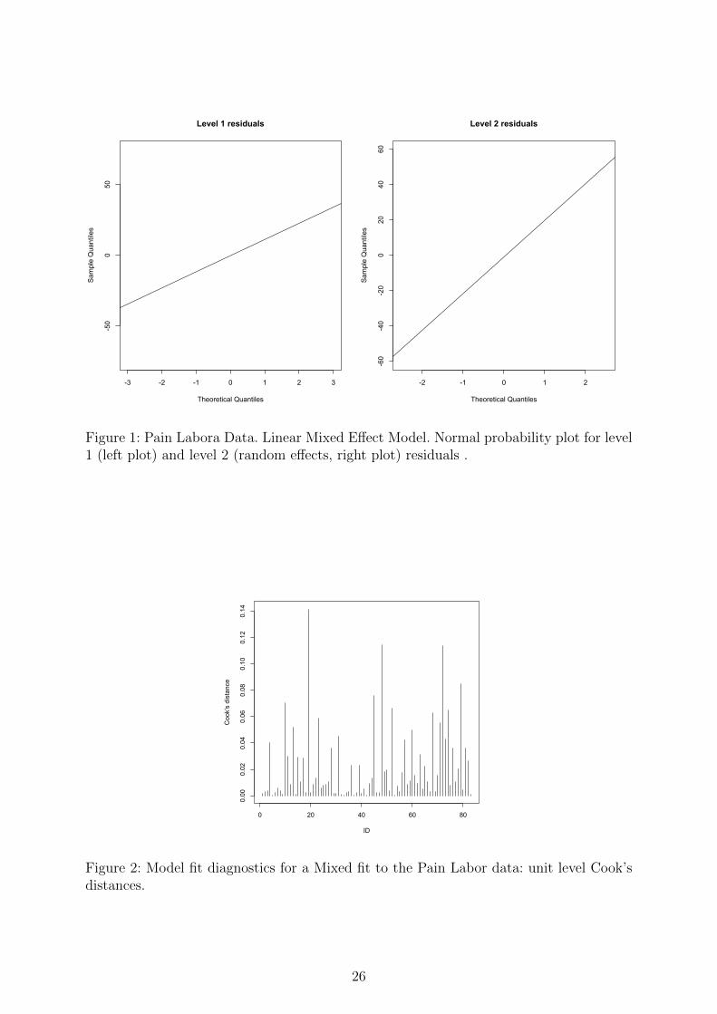
sign, over time. Figures 1 and 2 show selected diagnostics for a linear mixed model fit

to the response variable based on the original Pain Labor data using Treatment, Time

19

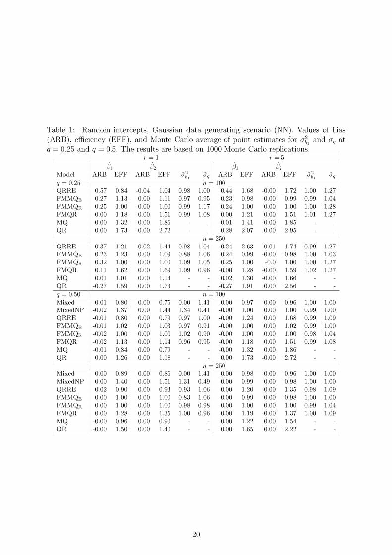
Table 1: Random intercepts, Gaussian data generating scenario (NN). Values of bias(ARB), efficiency (EFF), and Monte Carlo average of point estimates for σ2

b1and σq at

q = 0.25 and q = 0.5. The results are based on 1000 Monte Carlo replications.r = 1 r = 5

β1 β2 β1 β2Model ARB EFF ARB EFF ¯σ2

b1¯σq ARB EFF ARB EFF ¯σ2

b1¯σq

q = 0.25 n = 100QRRE 0.57 0.84 -0.04 1.04 0.98 1.00 0.44 1.68 -0.00 1.72 1.00 1.27FMMQE 0.27 1.13 0.00 1.11 0.97 0.95 0.23 0.98 0.00 0.99 0.99 1.04FMMQR 0.25 1.00 0.00 1.00 0.99 1.17 0.24 1.00 0.00 1.00 1.00 1.28FMQR -0.00 1.18 0.00 1.51 0.99 1.08 -0.00 1.21 0.00 1.51 1.01 1.27MQ -0.00 1.32 0.00 1.86 - - 0.01 1.41 0.00 1.85 - -QR 0.00 1.73 -0.00 2.72 - - -0.28 2.07 0.00 2.95 - -

n = 250QRRE 0.37 1.21 -0.02 1.44 0.98 1.04 0.24 2.63 -0.01 1.74 0.99 1.27FMMQE 0.23 1.23 0.00 1.09 0.88 1.06 0.24 0.99 -0.00 0.98 1.00 1.03FMMQR 0.32 1.00 0.00 1.00 1.09 1.05 0.25 1.00 -0.0 1.00 1.00 1.27FMQR 0.11 1.62 0.00 1.69 1.09 0.96 -0.00 1.28 -0.00 1.59 1.02 1.27MQ 0.01 1.01 0.00 1.14 - - 0.02 1.30 -0.00 1.66 - -QR -0.27 1.59 0.00 1.73 - - -0.27 1.91 0.00 2.56 - -q = 0.50 n = 100Mixed -0.01 0.80 0.00 0.75 0.00 1.41 -0.00 0.97 0.00 0.96 1.00 1.00MixedNP -0.02 1.37 0.00 1.44 1.34 0.41 -0.00 1.00 0.00 1.00 0.99 1.00QRRE -0.01 0.80 0.00 0.79 0.97 1.00 -0.00 1.24 0.00 1.68 0.99 1.09FMMQE -0.01 1.02 0.00 1.03 0.97 0.91 -0.00 1.00 0.00 1.02 0.99 1.00FMMQR -0.02 1.00 0.00 1.00 1.02 0.90 -0.00 1.00 0.00 1.00 0.98 1.04FMQR -0.02 1.13 0.00 1.14 0.96 0.95 -0.00 1.18 0.00 1.51 0.99 1.08MQ -0.01 0.84 0.00 0.79 - - -0.00 1.32 0.00 1.86 - -QR 0.00 1.26 0.00 1.18 - - 0.00 1.73 -0.00 2.72 - -

n = 250Mixed 0.00 0.89 0.00 0.86 0.00 1.41 0.00 0.98 0.00 0.96 1.00 1.00MixedNP 0.00 1.40 0.00 1.51 1.31 0.49 0.00 0.99 0.00 0.98 1.00 1.00QRRE 0.02 0.90 0.00 0.93 0.93 1.06 0.00 1.20 -0.00 1.35 0.98 1.09FMMQE 0.00 1.00 0.00 1.00 0.83 1.06 0.00 0.99 0.00 0.98 1.00 1.00FMMQR 0.00 1.00 0.00 1.00 0.98 0.98 0.00 1.00 0.00 1.00 0.99 1.04FMQR 0.00 1.28 0.00 1.35 1.00 0.96 0.00 1.19 -0.00 1.37 1.00 1.09MQ -0.00 0.96 0.00 0.90 - - 0.00 1.22 0.00 1.54 - -QR -0.00 1.50 0.00 1.40 - - 0.00 1.65 0.00 2.22 - -

20

Table 2: Random intercepts, t3 data generating scenario (TT). Values of bias (ARB),efficiency (EFF), and Monte Carlo average of point estimates for σ2

b1and σq at q = 0.25

and q = 0.5. The results are based on 1000 Monte Carlo replications.r = 1 r = 5

β1 β2 β1 β2Model ARB EFF ARB EFF ¯σ2

b1¯σq ARB EFF ARB EFF ¯σ2

b1¯σq

q = 0.25 n = 100QRRE 0.46 1.06 -0.06 1.09 1.01 2.25 -0.19 1.74 -0.00 0.98 1.55 2.37FMMQE 0.17 1.11 -0.00 0.98 1.71 1.38 0.00 1.08 0.00 1.32 1.61 1.55FMMQR 0.03 1.00 -0.00 1.00 1.31 1.88 0.00 1.00 0.00 1.00 1.61 1.92FMQR -0.29 1.11 -0.00 1.16 1.04 2.14 0.00 0.91 0.00 0.91 1.48 1.61MQ -0.13 0.98 -0.00 0.99 - - 0.00 0.83 0.00 1.51 - -QR -0.44 1.24 -0.00 1.28 - - 0.00 0.91 0.00 1.89 - -

n = 250QRRE 0.05 1.16 -0.03 1.29 1.05 2.22 0.09 1.43 -0.00 1.09 1.47 1.93FMMQE 0.12 1.11 -0.00 0.99 1.73 1.44 0.10 1.17 0.00 1.20 1.73 1.49FMMQR 0.05 1.00 -0.00 1.00 1.44 1.83 0.13 1.00 0.00 1.00 1.69 1.78FMQR -0.32 1.16 0.00 1.33 1.20 2.09 -0.15 0.91 0.00 0.96 1.54 1.96MQ -0.13 0.96 -0.00 1.07 - - -0.15 1.00 0.00 1.37 - -QR -0.43 1.26 -0.00 1.40 - - -0.44 1.16 0.00 1.77 - -q = 0.50 n = 100Mixed 0.01 1.40 -0.00 1.36 0.00 2.36 0.02 1.07 -0.00 1.12 1.64 1.68MixedNP 0.02 1.41 -0.00 1.50 2.19 0.81 0.02 1.08 -0.00 1.18 1.64 1.67QRRE 0.02 0.95 -0.00 0.93 0.61 2.09 0.00 1.67 -0.00 0.86 1.51 1.58FMMQE 0.02 1.15 -0.00 1.13 1.75 1.43 0.02 1.09 -0.00 1.19 1.62 1.63FMMQR 0.03 1.00 -0.00 1.00 0.90 1.73 0.01 1.00 -0.00 1.00 1.62 1.51FMQR 0.01 0.97 -0.00 0.99 0.56 2.11 0.01 0.84 -0.00 0.90 1.44 1.62MQ 0.02 0.85 -0.00 0.85 - - 0.00 0.83 -0.00 1.27 - -QR 0.03 1.07 -0.00 1.05 - - 0.00 0.95 0.00 1.62 - -

n = 250Mixed 0.01 1.36 -0.00 1.48 0.00 2.41 0.00 1.08 0.00 1.22 1.66 1.71MixedNP 0.02 1.17 -0.00 1.16 2.07 1.19 0.00 1.06 0.00 1.21 1.65 1.72QRRE 0.02 0.98 -0.00 1.04 0.63 2.13 -0.00 1.92 0.00 0.94 1.50 1.59FMMQE 0.01 1.07 -0.00 1.10 1.71 1.59 0.00 1.06 0.00 1.22 1.65 1.64FMMQR 0.02 1.00 -0.00 1.00 0.65 1.95 0.00 1.00 0.00 1.00 1.62 1.52FMQR 0.02 1.03 -0.00 1.10 0.56 2.16 0.00 0.90 0.00 0.90 1.45 1.62MQ 0.02 0.90 -0.00 0.95 - - 0.00 0.90 0.00 1.29 - -QR 0.01 1.12 -0.00 1.18 - - -0.00 0.96 0.00 1.65 - -

21

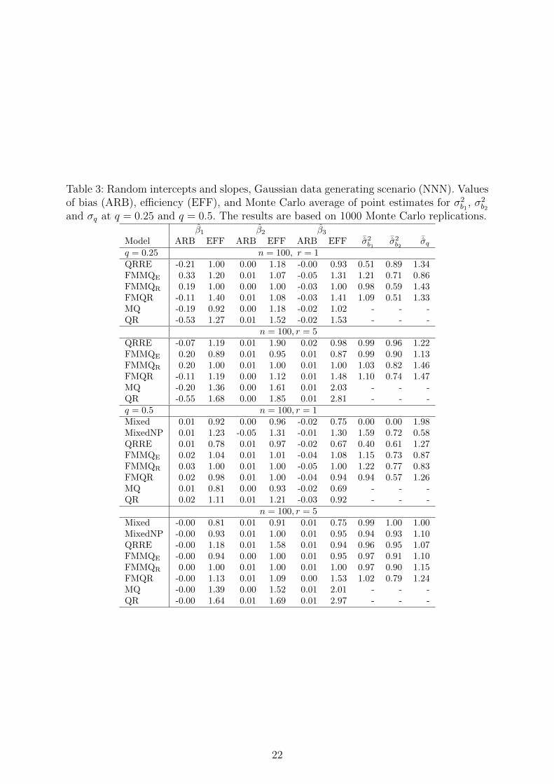
Table 3: Random intercepts and slopes, Gaussian data generating scenario (NNN). Valuesof bias (ARB), efficiency (EFF), and Monte Carlo average of point estimates for σ2

b1, σ2

b2

and σq at q = 0.25 and q = 0.5. The results are based on 1000 Monte Carlo replications.β1 β2 β3

Model ARB EFF ARB EFF ARB EFF ¯σ2b1

¯σ2b2

¯σqq = 0.25 n = 100, r = 1QRRE -0.21 1.00 0.00 1.18 -0.00 0.93 0.51 0.89 1.34FMMQE 0.33 1.20 0.01 1.07 -0.05 1.31 1.21 0.71 0.86FMMQR 0.19 1.00 0.00 1.00 -0.03 1.00 0.98 0.59 1.43FMQR -0.11 1.40 0.01 1.08 -0.03 1.41 1.09 0.51 1.33MQ -0.19 0.92 0.00 1.18 -0.02 1.02 - - -QR -0.53 1.27 0.01 1.52 -0.02 1.53 - - -

n = 100, r = 5QRRE -0.07 1.19 0.01 1.90 0.02 0.98 0.99 0.96 1.22FMMQE 0.20 0.89 0.01 0.95 0.01 0.87 0.99 0.90 1.13FMMQR 0.20 1.00 0.01 1.00 0.01 1.00 1.03 0.82 1.46FMQR -0.11 1.19 0.00 1.12 0.01 1.48 1.10 0.74 1.47MQ -0.20 1.36 0.00 1.61 0.01 2.03 - - -QR -0.55 1.68 0.00 1.85 0.01 2.81 - - -q = 0.5 n = 100, r = 1Mixed 0.01 0.92 0.00 0.96 -0.02 0.75 0.00 0.00 1.98MixedNP 0.01 1.23 -0.05 1.31 -0.01 1.30 1.59 0.72 0.58QRRE 0.01 0.78 0.01 0.97 -0.02 0.67 0.40 0.61 1.27FMMQE 0.02 1.04 0.01 1.01 -0.04 1.08 1.15 0.73 0.87FMMQR 0.03 1.00 0.01 1.00 -0.05 1.00 1.22 0.77 0.83FMQR 0.02 0.98 0.01 1.00 -0.04 0.94 0.94 0.57 1.26MQ 0.01 0.81 0.00 0.93 -0.02 0.69 - - -QR 0.02 1.11 0.01 1.21 -0.03 0.92 - - -

n = 100, r = 5Mixed -0.00 0.81 0.01 0.91 0.01 0.75 0.99 1.00 1.00MixedNP -0.00 0.93 0.01 1.00 0.01 0.95 0.94 0.93 1.10QRRE -0.00 1.18 0.01 1.58 0.01 0.94 0.96 0.95 1.07FMMQE -0.00 0.94 0.00 1.00 0.01 0.95 0.97 0.91 1.10FMMQR 0.00 1.00 0.01 1.00 0.01 1.00 0.97 0.90 1.15FMQR -0.00 1.13 0.01 1.09 0.00 1.53 1.02 0.79 1.24MQ -0.00 1.39 0.00 1.52 0.01 2.01 - - -QR -0.00 1.64 0.01 1.69 0.01 2.97 - - -

22

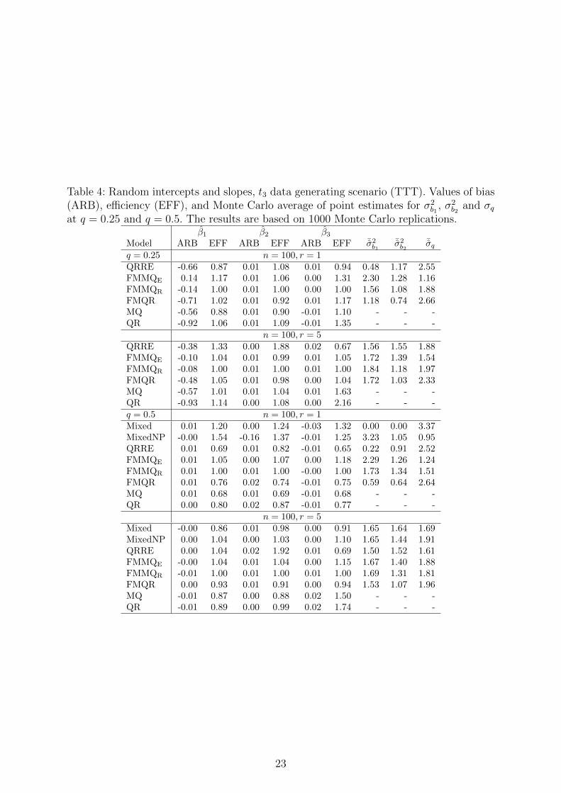
Table 4: Random intercepts and slopes, t3 data generating scenario (TTT). Values of bias(ARB), efficiency (EFF), and Monte Carlo average of point estimates for σ2

b1, σ2

b2and σq

at q = 0.25 and q = 0.5. The results are based on 1000 Monte Carlo replications.β1 β2 β3

Model ARB EFF ARB EFF ARB EFF ¯σ2b1

¯σ2b2

¯σqq = 0.25 n = 100, r = 1QRRE -0.66 0.87 0.01 1.08 0.01 0.94 0.48 1.17 2.55FMMQE 0.14 1.17 0.01 1.06 0.00 1.31 2.30 1.28 1.16FMMQR -0.14 1.00 0.01 1.00 0.00 1.00 1.56 1.08 1.88FMQR -0.71 1.02 0.01 0.92 0.01 1.17 1.18 0.74 2.66MQ -0.56 0.88 0.01 0.90 -0.01 1.10 - - -QR -0.92 1.06 0.01 1.09 -0.01 1.35 - - -

n = 100, r = 5QRRE -0.38 1.33 0.00 1.88 0.02 0.67 1.56 1.55 1.88FMMQE -0.10 1.04 0.01 0.99 0.01 1.05 1.72 1.39 1.54FMMQR -0.08 1.00 0.01 1.00 0.01 1.00 1.84 1.18 1.97FMQR -0.48 1.05 0.01 0.98 0.00 1.04 1.72 1.03 2.33MQ -0.57 1.01 0.01 1.04 0.01 1.63 - - -QR -0.93 1.14 0.00 1.08 0.00 2.16 - - -q = 0.5 n = 100, r = 1Mixed 0.01 1.20 0.00 1.24 -0.03 1.32 0.00 0.00 3.37MixedNP -0.00 1.54 -0.16 1.37 -0.01 1.25 3.23 1.05 0.95QRRE 0.01 0.69 0.01 0.82 -0.01 0.65 0.22 0.91 2.52FMMQE 0.01 1.05 0.00 1.07 0.00 1.18 2.29 1.26 1.24FMMQR 0.01 1.00 0.01 1.00 -0.00 1.00 1.73 1.34 1.51FMQR 0.01 0.76 0.02 0.74 -0.01 0.75 0.59 0.64 2.64MQ 0.01 0.68 0.01 0.69 -0.01 0.68 - - -QR 0.00 0.80 0.02 0.87 -0.01 0.77 - - -

n = 100, r = 5Mixed -0.00 0.86 0.01 0.98 0.00 0.91 1.65 1.64 1.69MixedNP 0.00 1.04 0.00 1.03 0.00 1.10 1.65 1.44 1.91QRRE 0.00 1.04 0.02 1.92 0.01 0.69 1.50 1.52 1.61FMMQE -0.00 1.04 0.01 1.04 0.00 1.15 1.67 1.40 1.88FMMQR -0.01 1.00 0.01 1.00 0.01 1.00 1.69 1.31 1.81FMQR 0.00 0.93 0.01 0.91 0.00 0.94 1.53 1.07 1.96MQ -0.01 0.87 0.00 0.88 0.02 1.50 - - -QR -0.01 0.89 0.00 0.99 0.02 1.74 - - -

23

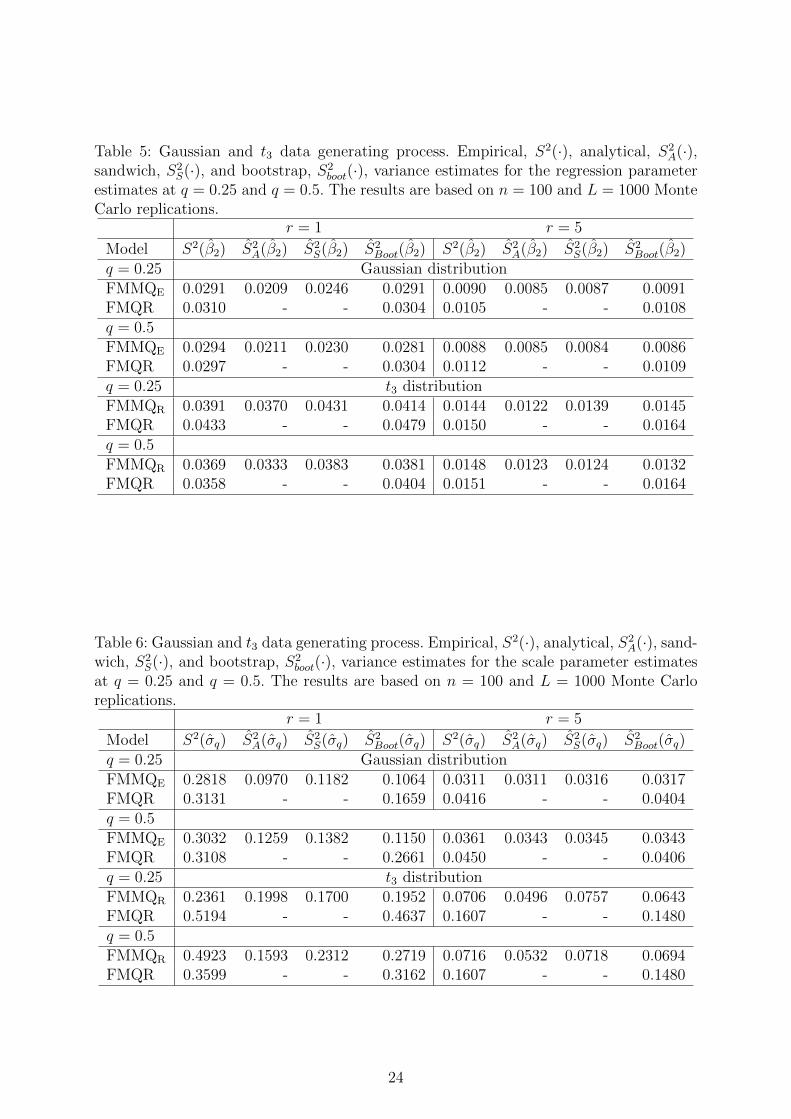
Table 5: Gaussian and t3 data generating process. Empirical, S2(·), analytical, S2A(·),

sandwich, S2S(·), and bootstrap, S2

boot(·), variance estimates for the regression parameterestimates at q = 0.25 and q = 0.5. The results are based on n = 100 and L = 1000 MonteCarlo replications.

r = 1 r = 5

Model S2(β2) S2A(β2) S2

S(β2) S2Boot(β2) S2(β2) S2

A(β2) S2S(β2) S2

Boot(β2)q = 0.25 Gaussian distributionFMMQE 0.0291 0.0209 0.0246 0.0291 0.0090 0.0085 0.0087 0.0091FMQR 0.0310 - - 0.0304 0.0105 - - 0.0108q = 0.5FMMQE 0.0294 0.0211 0.0230 0.0281 0.0088 0.0085 0.0084 0.0086FMQR 0.0297 - - 0.0304 0.0112 - - 0.0109q = 0.25 t3 distributionFMMQR 0.0391 0.0370 0.0431 0.0414 0.0144 0.0122 0.0139 0.0145FMQR 0.0433 - - 0.0479 0.0150 - - 0.0164q = 0.5FMMQR 0.0369 0.0333 0.0383 0.0381 0.0148 0.0123 0.0124 0.0132FMQR 0.0358 - - 0.0404 0.0151 - - 0.0164

Table 6: Gaussian and t3 data generating process. Empirical, S2(·), analytical, S2A(·), sand-

wich, S2S(·), and bootstrap, S2

boot(·), variance estimates for the scale parameter estimatesat q = 0.25 and q = 0.5. The results are based on n = 100 and L = 1000 Monte Carloreplications.

r = 1 r = 5

Model S2(σq) S2A(σq) S2

S(σq) S2Boot(σq) S2(σq) S2

A(σq) S2S(σq) S2

Boot(σq)q = 0.25 Gaussian distributionFMMQE 0.2818 0.0970 0.1182 0.1064 0.0311 0.0311 0.0316 0.0317FMQR 0.3131 - - 0.1659 0.0416 - - 0.0404q = 0.5FMMQE 0.3032 0.1259 0.1382 0.1150 0.0361 0.0343 0.0345 0.0343FMQR 0.3108 - - 0.2661 0.0450 - - 0.0406q = 0.25 t3 distributionFMMQR 0.2361 0.1998 0.1700 0.1952 0.0706 0.0496 0.0757 0.0643FMQR 0.5194 - - 0.4637 0.1607 - - 0.1480q = 0.5FMMQR 0.4923 0.1593 0.2312 0.2719 0.0716 0.0532 0.0718 0.0694FMQR 0.3599 - - 0.3162 0.1607 - - 0.1480

24

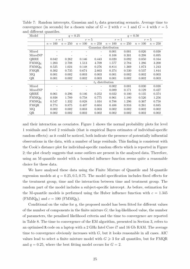
Table 7: Random intercepts, Gaussian and t3 data generating scenario. Average time toconvergence (in seconds) for a chosen value of G = 2 with r = 1 and G = 4 with r = 5and different quantiles.

Model q = 0.25 q = 0.50r = 1 r = 5 r = 1 r = 5

n = 100 n = 250 n = 100 n = 250 n = 100 n = 250 n = 100 n = 250Gaussian distribution

Mixed - - - - 0.001 0.001 0.026 0.038MixedNP - - - - 0.108 0.301 0.298 0.895QRRE 0.042 0.262 0.146 0.443 0.020 0.092 0.050 0.164FMMQE 1.203 2.708 1.513 4.709 1.577 2.784 1.286 3.200FMMQR 0.525 1.024 0.148 0.276 0.814 1.369 1.073 1.243FMQR 0.302 0.735 0.674 2.663 0.374 0.530 0.537 1.844MQ 0.001 0.002 0.003 0.003 0.001 0.002 0.002 0.003QR 0.001 0.002 0.002 0.003 0.001 0.002 0.002 0.003

t3 distributionMixed - - - - 0.002 0.001 0.030 0.038MixedNP - - - - 0.089 0.171 0.129 0.427QRRE 0.061 0.296 0.146 0.252 0.022 0.100 0.135 0.374FMMQE 0.938 1.789 0.758 0.775 0.961 1.180 0.526 1.256FMMQR 0.547 1.332 0.828 1.034 0.788 1.296 0.367 0.758FMQR 0.774 0.875 0.407 0.604 0.488 0.916 0.261 0.885MQ 0.002 0.002 0.003 0.003 0.002 0.002 0.002 0.002QR 0.002 0.002 0.002 0.002 0.002 0.002 0.002 0.002

and their interaction as covariates. Figure 1 shows the normal probability plots for level

1 residuals and level 2 residuals (that is empirical Bayes estimates of individual-specific

random effects): as it could be noticed, both indicate the presence of potentially influential

observations in the data, with a number of large residuals. This finding is consistent with

the Cook’s distance plot for individual-specific random effects which is reported in Figure

2; the plot clearly suggests that some outliers are present in the analysed data. Therefore,

using an M-quantile model with a bounded influence function seems quite a reasonable

choice for these data.

We have analysed these data using the Finite Mixture of Quantile and M-quantile

regression models at q = 0.25, 0.5, 0.75. The model specification includes fixed effects for

the treatment group, time and the interaction between time and treatment group. The

random part of the model includes a subject-specific intercept. As before, estimation for

the M-quantile models is performed using the Huber influence function with c = 1.345

(FMMQR) and c = 100 (FMMQE).

Conditional on the value for q, the proposed model has been fitted for different values

of the number of components in the finite mixture G; the log-likelihood value, the number

of parameters, the penalised likelihood criteria and the time to convergence are reported

in Table 8. The time to convergence of the EM algorithm, presented in Section 3, refers to

an optimised R code on a laptop with a 2 GHz Intel Core i7 and 16 Gb RAM. The average

time to convergence obviously increases with G, but it looks reasonable in all cases. AIC

values lead to select a finite mixture model with G > 3 for all quantiles, but for FMQR

and q = 0.25, where the best fitting model occurs for G = 2.

25

-3 -2 -1 0 1 2 3

-50

050

Level 1 residuals

Theoretical Quantiles

Sam

ple

Qua

ntile

s

-2 -1 0 1 2-60

-40

-20

020

4060

Level 2 residuals

Theoretical Quantiles

Sam

ple

Qua

ntile

s

Figure 1: Pain Labora Data. Linear Mixed Effect Model. Normal probability plot for level1 (left plot) and level 2 (random effects, right plot) residuals .

0 20 40 60 80

0.00

0.02

0.04

0.06

0.08

0.10

0.12

0.14

ID

Coo

k's

dist

ance

Figure 2: Model fit diagnostics for a Mixed fit to the Pain Labor data: unit level Cook’sdistances.

26

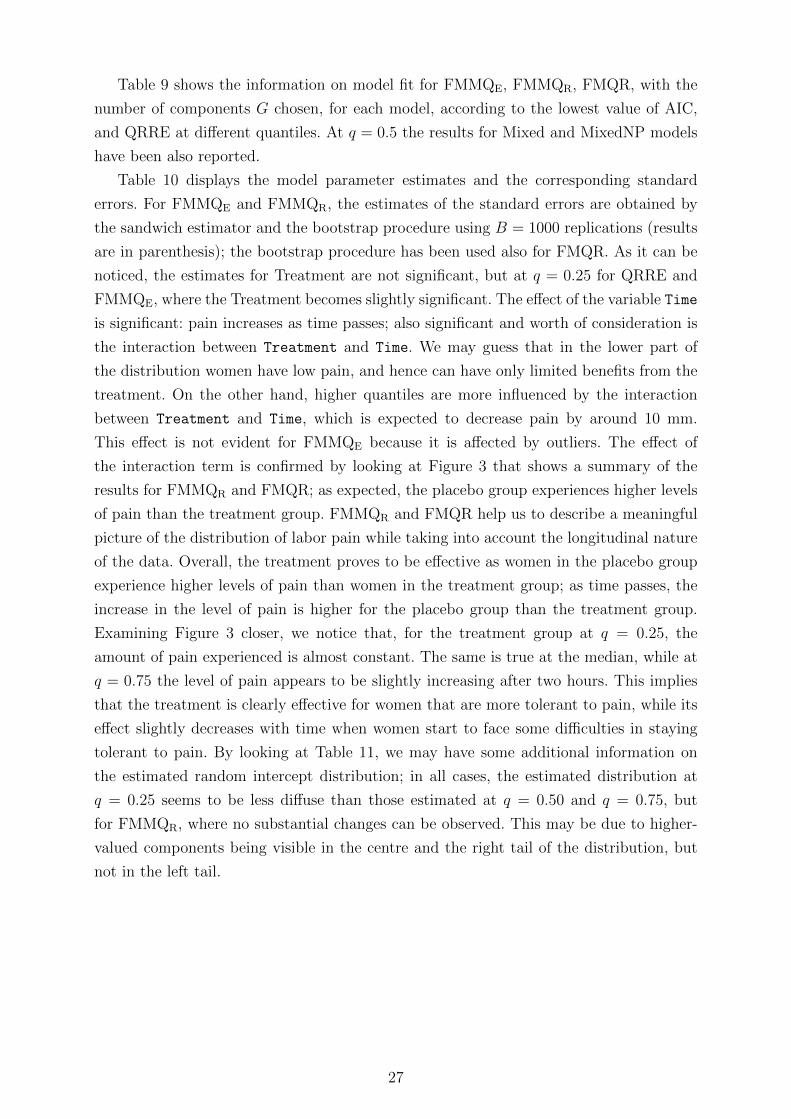
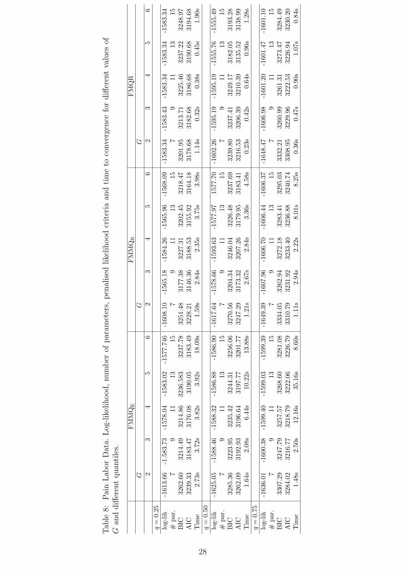
Table 9 shows the information on model fit for FMMQE, FMMQR, FMQR, with the

number of components G chosen, for each model, according to the lowest value of AIC,

and QRRE at different quantiles. At q = 0.5 the results for Mixed and MixedNP models

have been also reported.

Table 10 displays the model parameter estimates and the corresponding standard

errors. For FMMQE and FMMQR, the estimates of the standard errors are obtained by

the sandwich estimator and the bootstrap procedure using B = 1000 replications (results

are in parenthesis); the bootstrap procedure has been used also for FMQR. As it can be

noticed, the estimates for Treatment are not significant, but at q = 0.25 for QRRE and

FMMQE, where the Treatment becomes slightly significant. The effect of the variable Time

is significant: pain increases as time passes; also significant and worth of consideration is

the interaction between Treatment and Time. We may guess that in the lower part of

the distribution women have low pain, and hence can have only limited benefits from the

treatment. On the other hand, higher quantiles are more influenced by the interaction

between Treatment and Time, which is expected to decrease pain by around 10 mm.

This effect is not evident for FMMQE because it is affected by outliers. The effect of

the interaction term is confirmed by looking at Figure 3 that shows a summary of the

results for FMMQR and FMQR; as expected, the placebo group experiences higher levels

of pain than the treatment group. FMMQR and FMQR help us to describe a meaningful

picture of the distribution of labor pain while taking into account the longitudinal nature

of the data. Overall, the treatment proves to be effective as women in the placebo group

experience higher levels of pain than women in the treatment group; as time passes, the

increase in the level of pain is higher for the placebo group than the treatment group.

Examining Figure 3 closer, we notice that, for the treatment group at q = 0.25, the

amount of pain experienced is almost constant. The same is true at the median, while at

q = 0.75 the level of pain appears to be slightly increasing after two hours. This implies

that the treatment is clearly effective for women that are more tolerant to pain, while its

effect slightly decreases with time when women start to face some difficulties in staying

tolerant to pain. By looking at Table 11, we may have some additional information on

the estimated random intercept distribution; in all cases, the estimated distribution at

q = 0.25 seems to be less diffuse than those estimated at q = 0.50 and q = 0.75, but

for FMMQR, where no substantial changes can be observed. This may be due to higher-

valued components being visible in the centre and the right tail of the distribution, but

not in the left tail.

27

Tab

le8:

Pai

nL

abor

Dat

a.L

og-l

ikel

ihood,

num

ber

ofpar

amet

ers,

pen

alis

edlike

lihood

crit

eria

and

tim

eto

conve

rgen

cefo

rdiff

eren

tva

lues

ofG

and

diff

eren

tquan

tile

s.

FM

MQ

EF

MM

QR

FM

QR

GG

G2

34

56

23

45

62

34

56

q=

0.25

log-

lik

-161

3.66

-1.5

83.7

3-1

578.

04-1

583.

02-1

577.7

46

-1608.1

0-1

565.1

8-1

584.2

6-1

565.9

6-1

568.0

9-1

583.3

4-1

583.4

3-1

583.3

4-1

583.3

4-1

583.3

4#

par

.7

911

1315

79

11

13

15

79

11

13

15

BIC

3262

.60

3214

.49

3214

.86

3236

.583

3237.7

83251.4

83177.3

83227.3

13202.4

532

18.4

73201.9

53213.7

13225.4

63237.2

23248.9

7A

IC32

39.3

331

83.4

731

76.0

831

90.

0531

83.4

93228.2

13146.3

63188.5

33155.9

231

64.1

83178.6

83182.6

83186.6

83190.6

83194.6

8T

ime

2.73

s3.

72s

3.82

s3.

92s

18.0

9s

1.5

9s

2.8

4s

2.3

5s

3.7

5s

3.9

8s

1.1

4s

0.3

2s

0.3

8s

0.4

5s

1.9

0s

q=

0.50

log-

lik

-162

5.05

-158

8.46

-158

8.32

-158

6.88

-158

6.9

0-1

617.6

4-1

578.6

6-1

593.6

3-1

577.9

71577.7

0-1

602.2

6-1

595.1

9-1

595.1

9-1

555.7

6-1

555.4

9#

par

.7

911

1315

79

11

13

15

79

11

13

15

BIC

3285

.36

3223

.95

3235

.42

3244.

3132

56.0

63270.5

63204.3

43246.0

43226.4

832

37.6

93239.8

03237.4

13249.1

73182.0

53193.2

8A

IC32

62.0

931

92.9

331

96.6

431

97.

7732

01.7

73247.2

93173.3

23207.2

63179.9

531

83.4

13216.5

33206.3

93210.3

93135.5

23138.9

9T

ime

1.64

s2.

08s

6.44

s10

.22s

13.8

8s

1.2

1s

2.6

7s

2.8

4s

3.3

6s

4.5

8s

0.2

3s

0.4

2s

0.6

4s

0.9

6s

1.2

8s

q=

0.75

log-

lik

-163

6.01

-160

0.38

-159

9.40

-159

9.03

-159

9.3

9-1

649.3

9-1

607.9

6-1

606.7

0-1

606.4

4-1

606.3

7-1

648.4

7-1

606.9

8-1

601.2

0-1

601.4

7-1

601.1

0#

par

.7

911

1315

79

11

13

15

79

11

13

15

BIC

3307

.29

3247

.79

3257

.57

3268.

6032

81.0

83334.0

53262.9

43272.1

83283.4

132

95.0

33332.2

13260.9

93261.3

13273.4

73284.4

9A

IC32

84.0

232

16.7

732

18.7

932

22.

0632

26.7

93310.7

93231.9

23233.4

03236.8

832

40.7

43308.9

53229.9

63222.5

33226.9

43230.2

0T

ime

1.48

s2.

50s

12.1

6s35

.16s

8.6

0s

1.1

1s

2.9

4s

2.2

2s

8.0

1s

8.2

5s

0.3

6s

0.4

7s

0.9

0s

1.0

7s

0.8

4s

28

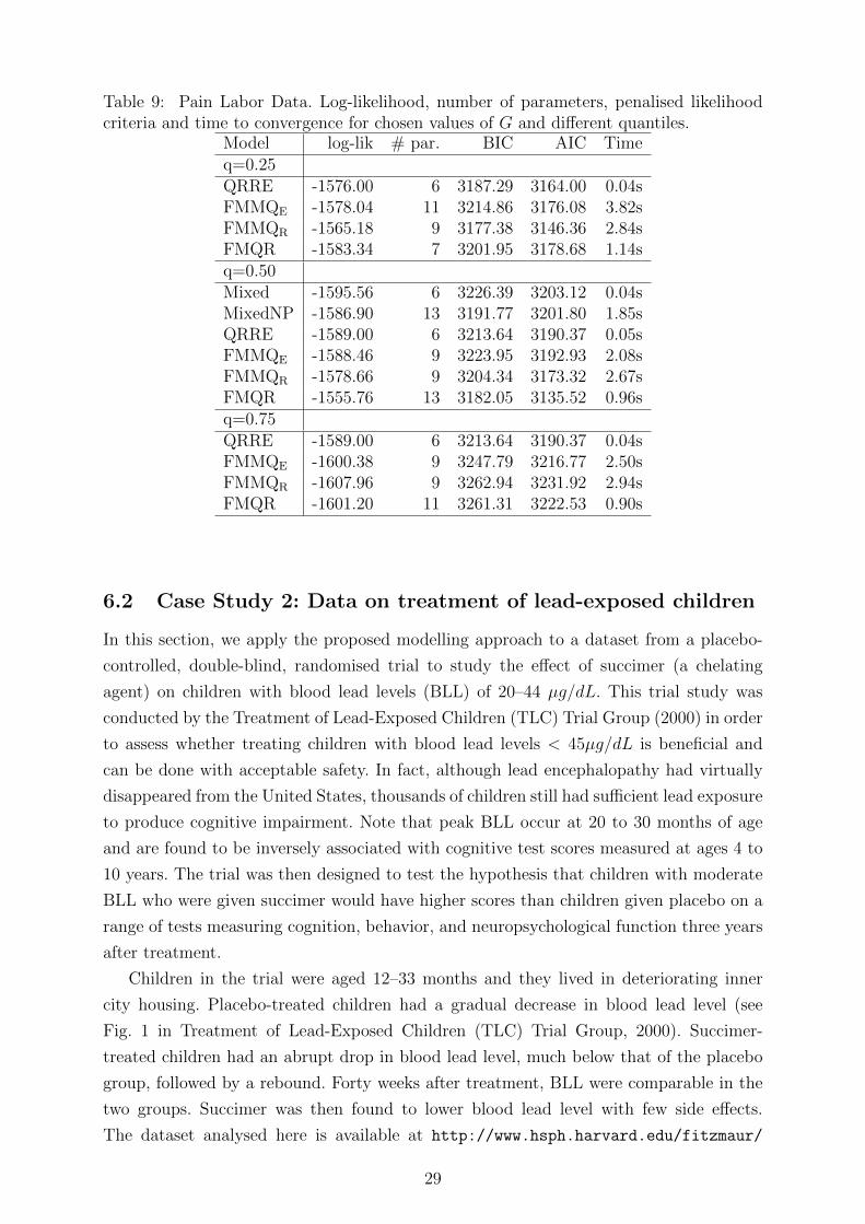
Table 9: Pain Labor Data. Log-likelihood, number of parameters, penalised likelihoodcriteria and time to convergence for chosen values of G and different quantiles.

Model log-lik # par. BIC AIC Timeq=0.25QRRE -1576.00 6 3187.29 3164.00 0.04sFMMQE -1578.04 11 3214.86 3176.08 3.82sFMMQR -1565.18 9 3177.38 3146.36 2.84sFMQR -1583.34 7 3201.95 3178.68 1.14sq=0.50Mixed -1595.56 6 3226.39 3203.12 0.04sMixedNP -1586.90 13 3191.77 3201.80 1.85sQRRE -1589.00 6 3213.64 3190.37 0.05sFMMQE -1588.46 9 3223.95 3192.93 2.08sFMMQR -1578.66 9 3204.34 3173.32 2.67sFMQR -1555.76 13 3182.05 3135.52 0.96sq=0.75QRRE -1589.00 6 3213.64 3190.37 0.04sFMMQE -1600.38 9 3247.79 3216.77 2.50sFMMQR -1607.96 9 3262.94 3231.92 2.94sFMQR -1601.20 11 3261.31 3222.53 0.90s

6.2 Case Study 2: Data on treatment of lead-exposed children

In this section, we apply the proposed modelling approach to a dataset from a placebo-

controlled, double-blind, randomised trial to study the effect of succimer (a chelating

agent) on children with blood lead levels (BLL) of 20–44 µg/dL. This trial study was

conducted by the Treatment of Lead-Exposed Children (TLC) Trial Group (2000) in order

to assess whether treating children with blood lead levels < 45µg/dL is beneficial and

can be done with acceptable safety. In fact, although lead encephalopathy had virtually

disappeared from the United States, thousands of children still had sufficient lead exposure

to produce cognitive impairment. Note that peak BLL occur at 20 to 30 months of age

and are found to be inversely associated with cognitive test scores measured at ages 4 to

10 years. The trial was then designed to test the hypothesis that children with moderate

BLL who were given succimer would have higher scores than children given placebo on a

range of tests measuring cognition, behavior, and neuropsychological function three years

after treatment.

Children in the trial were aged 12–33 months and they lived in deteriorating inner

city housing. Placebo-treated children had a gradual decrease in blood lead level (see

Fig. 1 in Treatment of Lead-Exposed Children (TLC) Trial Group, 2000). Succimer-

treated children had an abrupt drop in blood lead level, much below that of the placebo

group, followed by a rebound. Forty weeks after treatment, BLL were comparable in the

two groups. Succimer was then found to lower blood lead level with few side effects.

The dataset analysed here is available at http://www.hsph.harvard.edu/fitzmaur/

29

Table 10: Pain Labor Data. Parameter estimates and standard errors computed by sand-wich estimator. Standard errors in parenthesis are obtained by using 1000 bootstrapreplications.

Model q=0.25 q=0.50 q=0.75Variable Estimate Std. Error Estimate Std. Error Estimate Std. Error

Mixed

Treatement - - -11.15 6.03 - -Time - - 12.02 0.86 - -Treatement:Time - - -9.74 1.18 - -σb - - 24.22 - - -scale - - 16.44 - - -

MixedNP

Treatement - - 7.64 1.28 - -Time - - 11.22 0.35 - -Treatement:Time - - -9.05 0.47 - -σb - - 25.85 - - -scale - - 16.72 - - -

QRRE

Treatement -15.28 6.24 -7.63 6.47 -10.57 6.00Time 9.03 2.73 12.58 2.18 13.14 2.28Treatement:Time -9.03 2.81 -12.10 2.44 -11.97 2.94σb 15.78 18.26 18.35scale 18.23 17.16 20.27

FMMQE

Treatement -7.95 4.72 (4.32) 5.81 4.31 (6.43) 4.44 4.27 (8.10)Time 11.07 1.32 (1.79) 11.35 1.57 (1.53) 11.72 1.46 (1.52)Treatement:Time -9.90 1.48 (1.95) -9.23 1.88 (1.93) -9.16 1.89 (2.20)σb 21.82 25.14 26.20scale 14.69 16.86 15.56

FMMQR

Treatement 2.09 3.09 (3.81) 2.48 3.74 (6.88) -0.56 4.72 (9.75)Time 9.48 1.86 (1.52) 11.21 2.19 (2.58) 11.91 2.31(1.86)Treatement:Time -7.92 1.84 (2.72) -9.00 2.33 (2.38) -9.47 2.40 (2.50)σb 23.34 24.22 25.32scale 10.75 13.58 12.06

FMQR

Treatement 2.00 4.48 0.49 2.24 -3.50 9.90Time 9.00 3.03 9.24 2.89 14.25 2.93Treatement:Time -9.01 3.06 -8.74 2.93 -11.74 3.21σb 17.15 25.58 26.01scale 21.65 16.18 21.34

ala/tlc.txt and includes a subset of the original data for n = 100 children, 50 randomly

assigned to treatment (succimer) and 50 to placebo group. For each child, BLL is available

at baseline (or week 0), week 1, week 4 and week 6. This dataset has been reanalysed in

Geraci and Bottai (2014).

Geraci and Bottai (2014) show a selection of individual BLL trajectories: for most

children in the treatment group, a “U”-shaped curve describes the observed pattern,

with a rebound between 1 to 4 weeks of treatment with succimer. On the other hand, a

monotonic descending pattern can be mostly observed in the placebo group. The drop

in BLL after one week of treatment is much larger in the treatment group than the

slow decrease found in the placebo group. Given the observed “U”-shape, Geraci and

Bottai (2014) decided to model the temporal trajectories using natural cubic splines with

three degrees of freedom and knots placed at 0, 4 and 6 weeks. The B-spline basis has,

therefore, two components: T1 and T2, say. Here, we also consider a simpler quadratic

model to handle the observed patterns: in the following we will denote the linear and the

quadratic functions of time by time and time2.

Table 12 shows AIC values for a set of alternative models with several combinations

of fixed and subject-specific random parameters. Binary variable treat takes value 1

for children treated with succimer and 0 for children treated with placebo. Results are

displayed for models Mixed, QRRE, FMQR and FMMQR. The latter finite mixture models

30

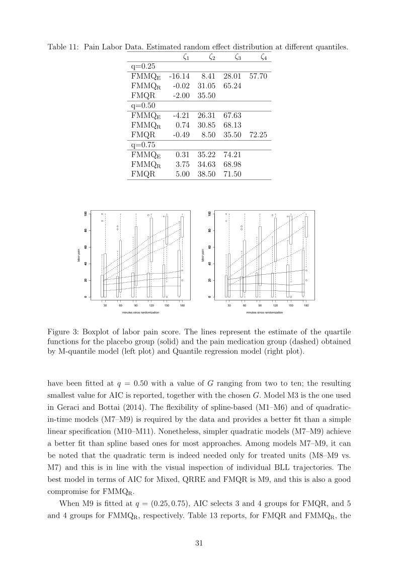
Table 11: Pain Labor Data. Estimated random effect distribution at different quantiles.ζ1 ζ2 ζ3 ζ4

q=0.25FMMQE -16.14 8.41 28.01 57.70FMMQR -0.02 31.05 65.24FMQR -2.00 35.50q=0.50FMMQE -4.21 26.31 67.63FMMQR 0.74 30.85 68.13FMQR -0.49 8.50 35.50 72.25q=0.75FMMQE 0.31 35.22 74.21FMMQR 3.75 34.63 68.98FMQR 5.00 38.50 71.50

020

4060

80100

minutes since randomization

labo

r pai

n

30 60 90 120 150 180

020

4060

80100

020

4060

80100

minutes since randomization

labo

r pai

n

30 60 90 120 150 180

020

4060

80100

Figure 3: Boxplot of labor pain score. The lines represent the estimate of the quartilefunctions for the placebo group (solid) and the pain medication group (dashed) obtainedby M-quantile model (left plot) and Quantile regression model (right plot).

have been fitted at q = 0.50 with a value of G ranging from two to ten; the resulting

smallest value for AIC is reported, together with the chosen G. Model M3 is the one used

in Geraci and Bottai (2014). The flexibility of spline-based (M1–M6) and of quadratic-

in-time models (M7–M9) is required by the data and provides a better fit than a simple

linear specification (M10–M11). Nonetheless, simpler quadratic models (M7–M9) achieve

a better fit than spline based ones for most approaches. Among models M7–M9, it can

be noted that the quadratic term is indeed needed only for treated units (M8–M9 vs.

M7) and this is in line with the visual inspection of individual BLL trajectories. The

best model in terms of AIC for Mixed, QRRE and FMQR is M9, and this is also a good

compromise for FMMQR.

When M9 is fitted at q = (0.25, 0.75), AIC selects 3 and 4 groups for FMQR, and 5

and 4 groups for FMMQR, respectively. Table 13 reports, for FMQR and FMMQR, the

31

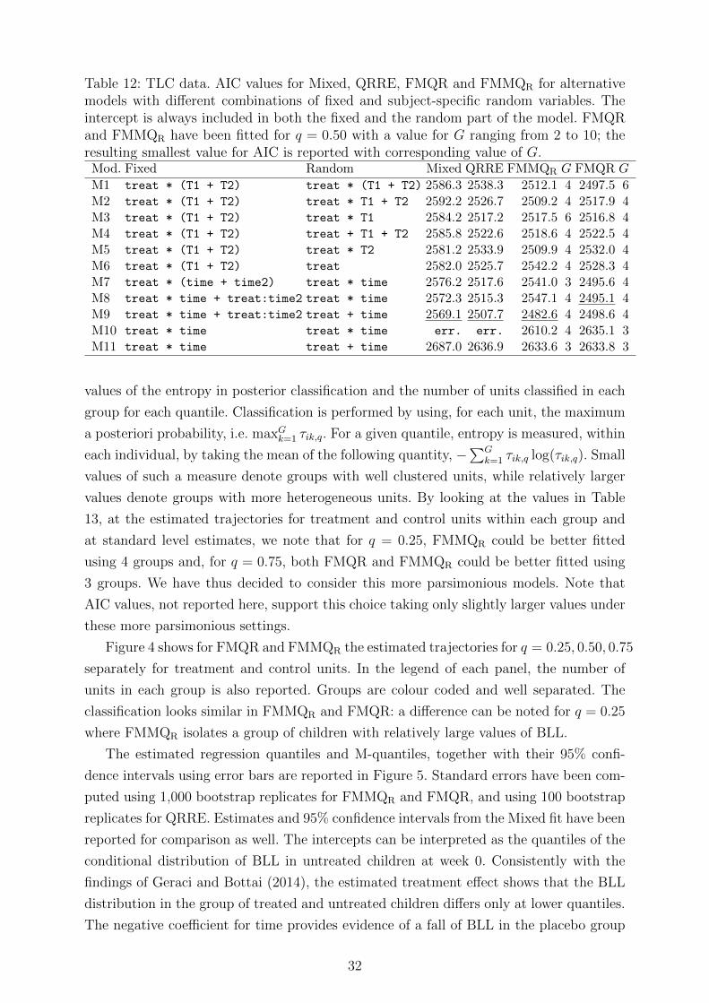
Table 12: TLC data. AIC values for Mixed, QRRE, FMQR and FMMQR for alternativemodels with different combinations of fixed and subject-specific random variables. Theintercept is always included in both the fixed and the random part of the model. FMQRand FMMQR have been fitted for q = 0.50 with a value for G ranging from 2 to 10; theresulting smallest value for AIC is reported with corresponding value of G.Mod. Fixed Random Mixed QRRE FMMQR G FMQR G

M1 treat * (T1 + T2) treat * (T1 + T2) 2586.3 2538.3 2512.1 4 2497.5 6M2 treat * (T1 + T2) treat * T1 + T2 2592.2 2526.7 2509.2 4 2517.9 4M3 treat * (T1 + T2) treat * T1 2584.2 2517.2 2517.5 6 2516.8 4M4 treat * (T1 + T2) treat + T1 + T2 2585.8 2522.6 2518.6 4 2522.5 4M5 treat * (T1 + T2) treat * T2 2581.2 2533.9 2509.9 4 2532.0 4M6 treat * (T1 + T2) treat 2582.0 2525.7 2542.2 4 2528.3 4M7 treat * (time + time2) treat * time 2576.2 2517.6 2541.0 3 2495.6 4M8 treat * time + treat:time2 treat * time 2572.3 2515.3 2547.1 4 2495.1 4M9 treat * time + treat:time2 treat + time 2569.1 2507.7 2482.6 4 2498.6 4M10 treat * time treat * time err. err. 2610.2 4 2635.1 3M11 treat * time treat + time 2687.0 2636.9 2633.6 3 2633.8 3

values of the entropy in posterior classification and the number of units classified in each

group for each quantile. Classification is performed by using, for each unit, the maximum

a posteriori probability, i.e. maxGk=1 τik,q. For a given quantile, entropy is measured, within

each individual, by taking the mean of the following quantity, −∑G

k=1 τik,q log(τik,q). Small

values of such a measure denote groups with well clustered units, while relatively larger

values denote groups with more heterogeneous units. By looking at the values in Table

13, at the estimated trajectories for treatment and control units within each group and

at standard level estimates, we note that for q = 0.25, FMMQR could be better fitted

using 4 groups and, for q = 0.75, both FMQR and FMMQR could be better fitted using

3 groups. We have thus decided to consider this more parsimonious models. Note that

AIC values, not reported here, support this choice taking only slightly larger values under

these more parsimonious settings.

Figure 4 shows for FMQR and FMMQR the estimated trajectories for q = 0.25, 0.50, 0.75

separately for treatment and control units. In the legend of each panel, the number of

units in each group is also reported. Groups are colour coded and well separated. The

classification looks similar in FMMQR and FMQR: a difference can be noted for q = 0.25

where FMMQR isolates a group of children with relatively large values of BLL.

The estimated regression quantiles and M-quantiles, together with their 95% confi-

dence intervals using error bars are reported in Figure 5. Standard errors have been com-

puted using 1,000 bootstrap replicates for FMMQR and FMQR, and using 100 bootstrap

replicates for QRRE. Estimates and 95% confidence intervals from the Mixed fit have been

reported for comparison as well. The intercepts can be interpreted as the quantiles of the

conditional distribution of BLL in untreated children at week 0. Consistently with the

findings of Geraci and Bottai (2014), the estimated treatment effect shows that the BLL

distribution in the group of treated and untreated children differs only at lower quantiles.

The negative coefficient for time provides evidence of a fall of BLL in the placebo group

32

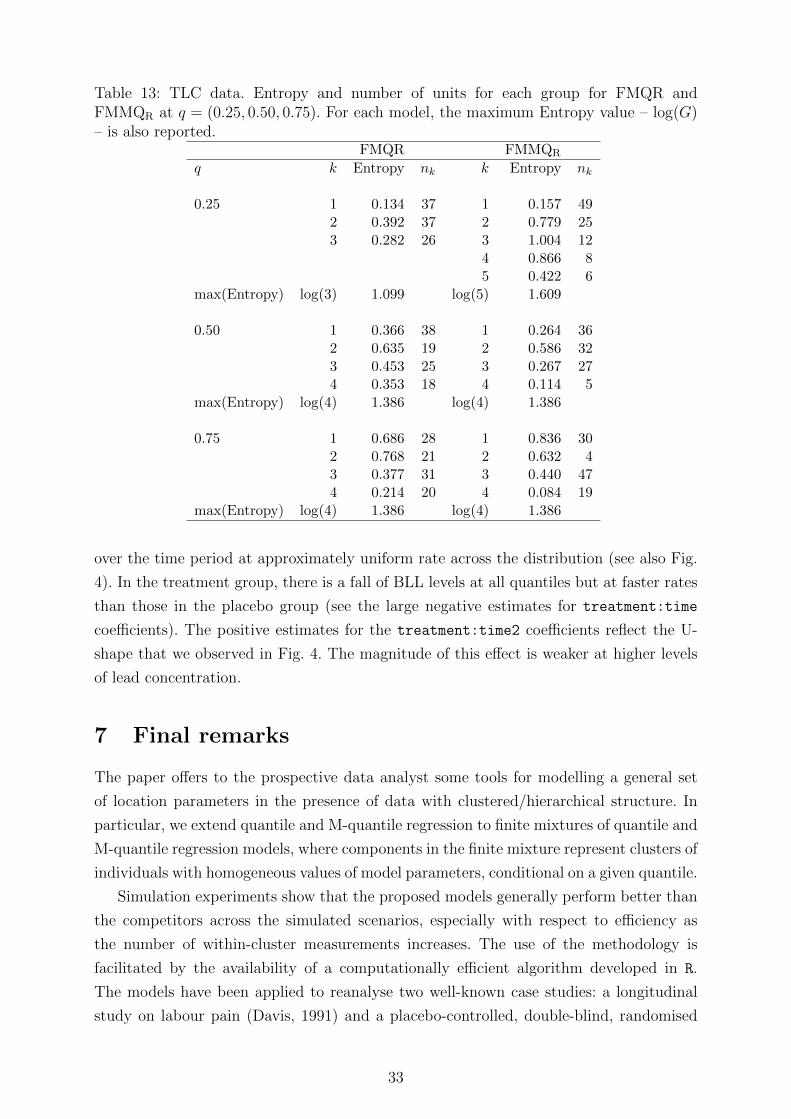
Table 13: TLC data. Entropy and number of units for each group for FMQR andFMMQR at q = (0.25, 0.50, 0.75). For each model, the maximum Entropy value – log(G)– is also reported.

FMQR FMMQR

q k Entropy nk k Entropy nk

0.25 1 0.134 37 1 0.157 492 0.392 37 2 0.779 253 0.282 26 3 1.004 12

4 0.866 85 0.422 6

max(Entropy) log(3) 1.099 log(5) 1.609

0.50 1 0.366 38 1 0.264 362 0.635 19 2 0.586 323 0.453 25 3 0.267 274 0.353 18 4 0.114 5

max(Entropy) log(4) 1.386 log(4) 1.386

0.75 1 0.686 28 1 0.836 302 0.768 21 2 0.632 43 0.377 31 3 0.440 474 0.214 20 4 0.084 19

max(Entropy) log(4) 1.386 log(4) 1.386

over the time period at approximately uniform rate across the distribution (see also Fig.

4). In the treatment group, there is a fall of BLL levels at all quantiles but at faster rates

than those in the placebo group (see the large negative estimates for treatment:time

coefficients). The positive estimates for the treatment:time2 coefficients reflect the U-

shape that we observed in Fig. 4. The magnitude of this effect is weaker at higher levels

of lead concentration.

7 Final remarks

The paper offers to the prospective data analyst some tools for modelling a general set

of location parameters in the presence of data with clustered/hierarchical structure. In

particular, we extend quantile and M-quantile regression to finite mixtures of quantile and

M-quantile regression models, where components in the finite mixture represent clusters of

individuals with homogeneous values of model parameters, conditional on a given quantile.

Simulation experiments show that the proposed models generally perform better than

the competitors across the simulated scenarios, especially with respect to efficiency as

the number of within-cluster measurements increases. The use of the methodology is

facilitated by the availability of a computationally efficient algorithm developed in R.

The models have been applied to reanalyse two well-known case studies: a longitudinal

study on labour pain (Davis, 1991) and a placebo-controlled, double-blind, randomised

33

0 1 2 3 4 5 6

510

1520

2530

FMQR q=0.25

time

BLL

T1−17T2−19T3−14C1−20C2−18C3−12

0 1 2 3 4 5 6

510

1520

2530

35

FMMQ q=0.25

time

BLL

T1−26T2−14T3−7T4−3C1−23C2−14C3−11C4−2

0 1 2 3 4 5 6

1015

2025

3035

FMQR q=0.50

time

BLL

T1−19T2−9T3−16T4−6C1−19C2−10C3−9C4−12

0 1 2 3 4 5 6

1015

2025

3035

FMMQ q=0.50

time

BLL

T1−16T2−16T3−15T4−3C1−20C2−16C3−12C4−2

0 1 2 3 4 5 6

1520

2530

35

FMQR q=0.75

time

BLL

T1−25T2−18T3−7C1−26C2−12C3−12

0 1 2 3 4 5 6

1015

2025

3035

FMMQ q=0.75

time

BLL

T1−16T2−27T3−7C1−20C2−18C3−12

Figure 4: TLC data. Estimated trajectories for FMMQR and FMQR at q = 0.25, 0.50, 0.75for each group identified with the mixtures and separately for the treatment (solid curves)and the control (dashed lines) group. Lines are colour coded according to the group andthe number of units belonging to each category is reported in the legend.

34

●

●

●

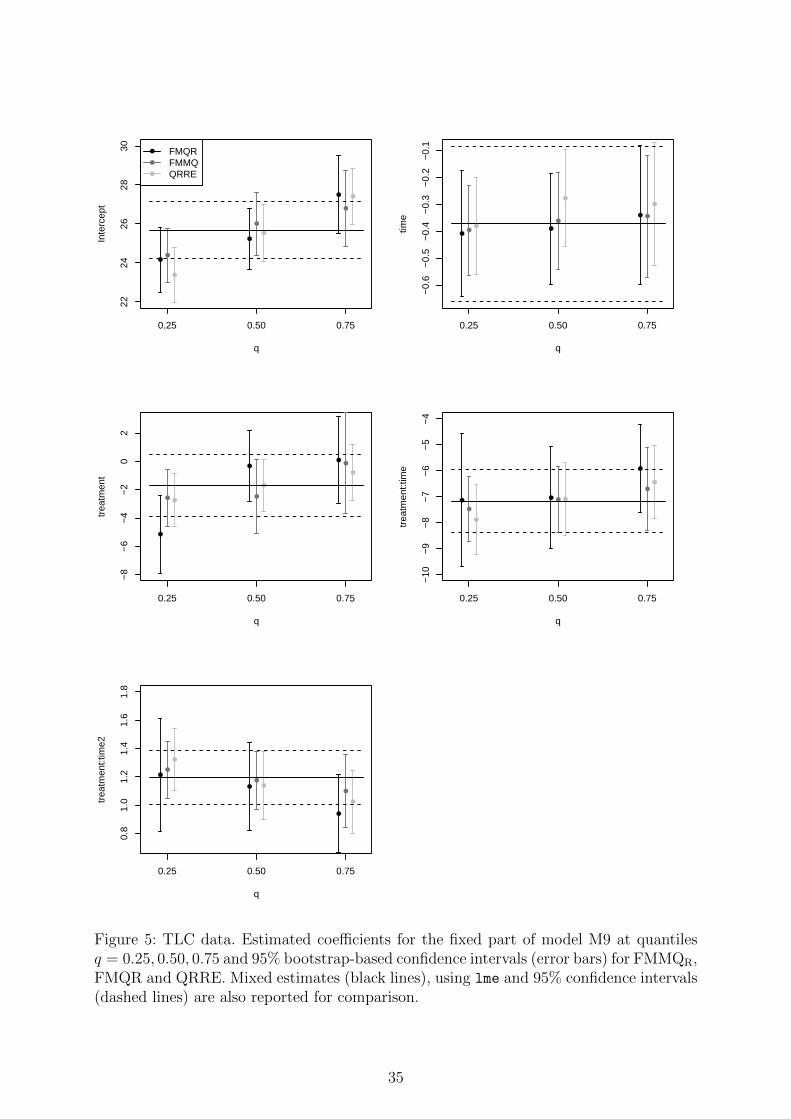
2224

2628

30

q

Inte

rcep

t

0.25 0.50 0.75

●

●

●

●

●

●

●

●

●

FMQRFMMQQRRE

●●

●

−0.

6−

0.5

−0.

4−

0.3

−0.

2−

0.1

q

time

0.25 0.50 0.75

●

●●

●

●●

●

●●

−8

−6

−4

−2

02

q

trea

tmen

t

0.25 0.50 0.75

● ●

●

●

●

●

● ●

●

−10

−9

−8

−7

−6

−5

−4

q

trea

tmen

t:tim

e

0.25 0.50 0.75

●

●

●

●

●

●

●

●

●

0.8

1.0

1.2

1.4

1.6

1.8

q

trea

tmen

t:tim

e2

0.25 0.50 0.75

●

●

●

●

●

●

Figure 5: TLC data. Estimated coefficients for the fixed part of model M9 at quantilesq = 0.25, 0.50, 0.75 and 95% bootstrap-based confidence intervals (error bars) for FMMQR,FMQR and QRRE. Mixed estimates (black lines), using lme and 95% confidence intervals(dashed lines) are also reported for comparison.

35

trial entailing children with blood lead levels (BLL) of 20–44 µg/dL (Treatment of Lead-

Exposed Children (TLC) Trial Group, 2000). The results of the two studies show the

capacity of the models to be adapted to different kinds of applications: random intercepts

for the first case and general random coefficients in the second study.

The proposed techniques envision a whole modelling framework that ex-

tends in various directions existing statistical models. First of all, by suitably

setting the tuning constant c to a relatively large value, it is possible to ex-

tend the classical finite mixture of linear regression models beyond the mean

within the expectile framework. On the other hand, when q = 0.5, the choice

of a relatively small value for the tuning constant c allows for a robust M-type

extension of the classical finite mixture of linear regression models that can

handle the presence of outlying observations. This robustification can also go

beyond the mean and pertain the other expectiles of the conditional distri-

bution of the response given the covariates. The important role of the tuning

constant c also envisions new research towards the development of estima-

tion strategies that allow for the joint estimation of its value and of model

parameters.

The introduction of a nonparametric distribution for the random effects

represents an important tool to further robustify M-quantile regression to

model misspecification. Recently, Tzavidis et al. (2015) have proposed a new approach

called M-quantile random effect regression, for modelling multilevel data. This method-

ology allows the estimation of a 2-level random intercept model. A line of research may

be to compare the performance of this new method with a finite mixture of M-quantile

models. In addition, given the particularly valuable contribution of finite mix-

tures in generalised linear modelling, it will be interesting to extend them

in an expectile and M-quantile fashion. Finally, extension to the multivariate

case is also on the agenda, although the development could be hindered by

the definition of expectiles and M-quantiles in more than one dimension.

Acknowledgements

The work of Salvati and Ranalli has been developed under the support of the

project PRIN-SURWEY http://www.sp.unipg.it/surwey/ (grant 2012F42NS8,

Italy).

References

Abramowitz, M. and Stegun, I. (1964). Handbook of Mathematical Functions. National

Bureau of standards, Washington DC.

36

Aitkin, M. (1996). A General Maximum Likelihood analysis of Overdispersion in Gener-

alized Linear Models. Statistics and Computing, 6:127–130.

Aitkin, M. (1999). A General Maximum Likelihood analysis of Variance Components in

Generalized Linear Models. Biometrics, 55:117–128.

Aitkin, M., Francis, B., and Hinde, J. (2005). Statistical Modelling in GLIM. Oxford

University Press 2nd edition.

Alfo, M. and Trovato, G. (2004). Semiparametric mixture models for multivariate count

data, with application. Econometrics Journal, 7:426–454.

Bianchi, A., Fabrizi, E., Salvati, N., and Tzavidis, N. (2015). M-quantile regression:

diagnostics and parametric representation of the model. Working paper, available at

http://www.sp.unipg.it/surwey/dowload/publications/24-mq-diagn.html.

Bianchi, A. and Salvati, N. (2015). Asymptotic properties and variance estimators of the

M-quantile regression coefficients estimators. Communications in Statistics - Theory

and Methods, 44:2416–2429.

Breckling, J. and Chambers, R. (1988). M -quantiles. Biometrika, 75:761–771.

Cantoni, E. and Ronchetti, E. (2001). Robust Inference for Generalized Linear Models.

Journal of the American Statistical Association, 96:1022–1030.

Davis, C. (1991). Semi-parametric and non-parametric methods for the analysis of

repeated measurements with applications to clinical trials. Statistics in Medicine,

10:1959–1980.

DeSarbo, W. and Cron, W. (1988). A maximum likelihood methodology for clusterwise

regression. Journal of Classification, 5:249–282.

Farcomeni, A. (2012). Quantile regression for longitudinal data based on latent Markov

subject-specific parameters. Statistics and Computing, 22:141–152.

Follmann, D. and Lambert, D. (1989). Generalizing logistic regression by nonparametric

mixing. Journal of the American Statistical Association, 84:295–300.

Friedl, H. and Kauermann, G. (2000). Standard errors for EM estimates in generalized

linear models with random effects. Biometrics, 56:761–767.

Geraci, M. and Bottai, M. (2007). Quantile regression for longitudinal data using the

asymmetric Laplace distribution. Biostatistics, 8:140–154.

Geraci, M. and Bottai, M. (2014). Linear quantile mixed models. Statistics and Comput-

ing, 24:461–479.

37

Geyer, C. and Thompson, E. (1992). Constrained Monte Carlo maximum likelihood for

dependent data. Journal of the Royal Statistical Society B, 54:657–699.

Gueorguieva, R. (2001). A multivariate generalized linear mixed model for joint modelling

of clustered outcomes in the exponential family. Statistical Modelling, 1:177–193.

Hennig, C. (2000). Identifiability of models for clusterwise linear regression. Journal of

Classification, 17:273–296.

Huber, P. (1964). Robust estimation of a location parameter. Ann. Math. Stat., 35:73–101.

Huber, P. (1973). Robust Regression: Asymptotics, Conjectures and Monte Carlo. The

Annals of Statistics, 1:799–821.

Huber, P. J. (1967). The behavior of maximum likelihood estimates under nonstandard

conditions. In Proceedings of the Fifth Berkeley Symposium on Mathematical Statistics

and Probability, pages 221–233. North Holland: Amsterdam.

Huber, P. J. (1981). Robust Statistics. John Wiley & Sons.

Jank, W. and Booth, J. (2003). Efficiency of Monte Carlo EM and Simulated Maximum

Likelihood in Two-Stage Hierarchical Models. Journal of Computational and Graphical

Statistics, 12:214–229.

Jones, M. C. (1994). Expectiles and m-quantiles are quantiles. Statistics and Probability

Letters, 20:149–153.

Jung, S. (1996). Quasi-likelihood for median regression models. Journal of the American

Statistical Association, 91:251–257.

Koenker, R. (2004). Quantile regression for longitudinal data. Journal of Multivariate

Analysis, 91:74–89.

Koenker, R. and Bassett, G. (1978). Regression quantiles. Econometrica, 46:33–50.

Koenker, R. and D’Orey, V. (1987). Computing regression quantiles. Biometrika, 93:255–

268.

Kokic, P., Chambers, R., Breckling, J., and Beare, S. (1997). A measure of production

performance. Journal of Business and Economic Statistics, 10:419–435.

Laird, N. M. (1978). Nonparametric maximum likelihood estimation of a mixing distri-

bution. Journal of the American Statistical Association, 73:805–811.

Lipsitz, S., Fitzmaurice, G., Molenberghs, G., and Zhao, L. (1997). Quantile regression

methods for longitudinal data with drop-outs: application to cd4 cell counts of patients

infected with the human immunodeficiency virus. Journal of the Royal Statistical soci-

ety, series C, 46:463–476.

38

Liu, Q. and Pierce, D. (1994). A note on Gaussian-Hermite quadrature. Biometrika,

81:624–629.

Liu, Y. and Bottai, M. (2009). Mixed-effects models for conditional quantiles with longi-

tudinal data. Internation Journal of Biostatistics, 5:1–22.

Louis, T. (1982). Finding the Observed information Matrix when Using the EM algorithm.

Journal of the Royal Statistical Society, Series B, 44:226–233.

McCulloch, C. (1994). Maximum likelihood estimation of variance components for binary

data. Journal of the American Statistical Association, 89:330–335.

Munkin, M. K. and Trivedi, P. K. (1999). Simulated maximum likelihood estimation

of multivariate mixed-Poisson regression models, with application. The Econometrics

Journal, 2:29–48.

Newey, W. and Powell, J. (1987). Asymmetric least squares estimation and testing.

Econometrica, 55:819–847.

Oakes, D. (1999). Direct Calculation of the Information Matrix via the EM Algorithm.

Journal of the Royal Statistical Society, series B, 61:479–482.

Pinheiro, J. and Bates, D. (1995). Approximations to the Log-Likelihood Function in the

Nonlinear Mixed-Effects Model. Journal of Computational and Graphical Statistics,

4:12–35.

Press, W., Teukolsky, S., Vetterling, W., and Flannery, B. (2007). Numerical recipes: the

art of scientific computing. New York: Cambridge University Press.

Salvati, N., Tzavidis, N., Pratesi, M., and Chambers, R. (2012). Small area estimation

via M-quantile geographically weighted regression. TEST, 21:1–28.

Street, J., Carroll, R., and Ruppert, D. (1988). A note on computing robust regression

estimates via iteratively reweighed least squares. The American Statistician, 42:152–

154.

Treatment of Lead-Exposed Children (TLC) Trial Group (2000). Safety and efficacy of

succimer in toddlers with blood lead levels of 20-44 µg/dl. Pediatr. Res., 48:593–599.

Tzavidis, N., Salvati, N., Schmid, T., Flouri, E., and Midouhas, E. (2015). Longitudinal

analysis of the Strengths and Difficulties Questionnaire scores of the Millennium Cohort

Study children in England using M-quantile random effects regression. Journal of the

Royal Statistical Society A, in press.

Wang, P., Puterman, M., Cockburn, I., and Le, N. (1996). Mixed Poisson regression

models with covariate dependent rates. Biometrics, 52:381–400.

39

Wang, Y., Lin, X., Zhu, M., and Bai, Z. (2007). Robust estimation using the huber fun-

tion with a data-dependent tuning constant. Journal of Computational and Graphical

Statistics, 16 (2):468–481.

Wedel, M. and DeSarbo, W. (1995). A mixture likelihood approach for generalized linear

models. Journal of Classification, 12:21–55.

White, H. (1980). A Heteroskedasticity-Consistent Covariance Matrix Estimator and a

Direct Test for Heteroskedasticity. Econometrica, 48:817–838.

40