RESOURCES ALLOCATION IN INDOORAND UNDERWATER VLC NETWORKS

BY

KHALED ABDUL-AZIZ AL-UTAIBI

A Dissertation Presented to theDEANSHIP OF GRADUATE STUDIES

In Partial Fulfillment of the Requirementsfor the Degree of

DOCTOR OF PHILOSOPHY

IN

COMPUTER SCIENCE ENGINEERING

KING FAHD UNIVERSITYOF PETROLEUM & MINERALS

Dhahran, Saudi Arabia

APRIL, 2019

KING FAHD UNIVERSITY OF PETROLEUM & MINERALSDHAHRAN 31261, SAUDI ARABIA

DEANSHIP OF GRADUATE STUDIES

This dissertation, written by KHALED ABDUL-AZIZ AL-UTAIBI under thedirection of his dissertation adviser and approved by his dissertation committee, hasbeen presented to and accepted by the Dean of Graduate Studies, in partial fulfill-ment of the requirements for the degree of DOCTOR OF PHILOSOPHY INCOMPUTER SCIENCE ENGINEERING.

Dissertation Committee

Dr. Sadiq M. Sait (Adviser)

Dr. Saad Al-Ahmadi (Member)

Dr. Aiman El-Maleh (Member)

Dr. Moataz Ahmad (Member)

Dr. Murat Uysal (Member)

Dr. Ahmad Al-MulhemDepartment Chairman

Dr. Salam A. ZummoDean of Graduate Studies

Date

©Khaled A. Al-Utaibi2019

iv

To the memory of my father and to my mother.

v

ACKNOWLEDGMENTS

Acknowledgement due to King Fahd University of Petroleum & Minerals for supporting

this research. I would like to express my appreciation to my dissertation advisor

Dr. Sadiq Sait Mohammed for his guidance, patience, and sincere advice throughout this

work. I acknowledge him for his valuable time, constructive criticism, and stimulating

discussions. Thanks are also due to my dissertation committee members, Dr. Saad

Al-Ahmadi, Dr. Aiman El-Maleh, Dr. Moataz Ahmad, and Dr. Murat Uysal for their

comments and critical review of the dissertation. I am very thankful to the Department

Chairman Dr. Ahmad Al-Mulhem and department secretary for their cooperation and

support.

vi

TABLE OF CONTENTS

ACKNOWLEDGMENTS vi

LIST OF TABLES x

LIST OF FIGURES xi

LIST OF SYMBOLS xiii

ABSTRACT (ENGLISH) xv

ABSTRACT (ARABIC) xvii

CHAPTER 1 BACKGROUND OF VLC SYSTEMS 1

1.1 Indoor of VLC Systems . . . . . . . . . . . . . . . . . . . . . . . . . . 5

1.1.1 Channel Modeling . . . . . . . . . . . . . . . . . . . . . . . . . 7

1.1.2 Path Loss Model . . . . . . . . . . . . . . . . . . . . . . . . . . 14

1.2 Underwater VLC Systems . . . . . . . . . . . . . . . . . . . . . . . . . 14

1.2.1 Path Loss Model . . . . . . . . . . . . . . . . . . . . . . . . . . 16

1.2.2 Turbulence Channel Model . . . . . . . . . . . . . . . . . . . . 18

1.3 Modulation Techniques . . . . . . . . . . . . . . . . . . . . . . . . . . . 18

1.3.1 On-Off Keying (OOK) . . . . . . . . . . . . . . . . . . . . . . . 19

1.3.2 Pulse Modulation Methods . . . . . . . . . . . . . . . . . . . . 19

1.3.3 Orthogonal Frequency Division Multiplexing (OFDM) . . . . . 22

1.3.4 Color Shift Keying (CSK) . . . . . . . . . . . . . . . . . . . . . 25

1.4 Multiple Access . . . . . . . . . . . . . . . . . . . . . . . . . . . . . . . 25

vii

CHAPTER 2 PROBLEM DEFINITION AND RESEARCH OBJEC-

TIVES 32

2.1 Literature Review . . . . . . . . . . . . . . . . . . . . . . . . . . . . . . 32

2.1.1 Handover . . . . . . . . . . . . . . . . . . . . . . . . . . . . . . 33

2.1.2 Load Balancing . . . . . . . . . . . . . . . . . . . . . . . . . . . 34

2.1.3 Resource Allocation . . . . . . . . . . . . . . . . . . . . . . . . 35

2.2 Dynamic LED Allocation Problem . . . . . . . . . . . . . . . . . . . . 37

2.2.1 LED Allocation for Indoor C-LiAN . . . . . . . . . . . . . . . . 37

2.2.2 Sensor Allocation for Underwater C-LiAN . . . . . . . . . . . . 41

2.3 Problem Definition . . . . . . . . . . . . . . . . . . . . . . . . . . . . . 44

2.4 Motivation . . . . . . . . . . . . . . . . . . . . . . . . . . . . . . . . . . 46

2.5 Research Objectives . . . . . . . . . . . . . . . . . . . . . . . . . . . . 47

CHAPTER 3 THE TETRIS GAME MODEL 48

3.1 The Tetris Game . . . . . . . . . . . . . . . . . . . . . . . . . . . . . . 49

3.2 The Tetris Model . . . . . . . . . . . . . . . . . . . . . . . . . . . . . . 51

3.2.1 Tetris Pieces . . . . . . . . . . . . . . . . . . . . . . . . . . . . 51

3.2.2 Solution Representation . . . . . . . . . . . . . . . . . . . . . . 51

3.2.3 Extended Solution Representation . . . . . . . . . . . . . . . . 59

3.3 Generating Tetris Pieces . . . . . . . . . . . . . . . . . . . . . . . . . . 61

3.4 Placement of Pieces . . . . . . . . . . . . . . . . . . . . . . . . . . . . . 62

CHAPTER 4 OPTIMIZATION HEURISTICS BASED ON TETRIS

GAME MODEL 64

4.1 Initial Solution Generation . . . . . . . . . . . . . . . . . . . . . . . . . 64

4.2 Simulated Annealing . . . . . . . . . . . . . . . . . . . . . . . . . . . . 65

4.3 Implementation Details . . . . . . . . . . . . . . . . . . . . . . . . . . . 66

4.3.1 The Neighbor Function . . . . . . . . . . . . . . . . . . . . . . 67

4.3.2 The Cost Function . . . . . . . . . . . . . . . . . . . . . . . . . 67

viii

CHAPTER 5 NUMERICAL RESULTS AND DISCUSSION 82

5.1 Indoor RA Optimization . . . . . . . . . . . . . . . . . . . . . . . . . . 82

5.1.1 System Throughput Vs Number of Users . . . . . . . . . . . . . 83

5.1.2 System Throughput Vs Number of Iterations . . . . . . . . . . 83

5.2 Underwater RA Optimization . . . . . . . . . . . . . . . . . . . . . . . 87

5.3 Results Discussion and Future Work . . . . . . . . . . . . . . . . . . . 87

APPENDIX A SUPPLEMENTARY MATERIAL 95

A.1 MATLAB Code: Direct Application Simulated Annealing . . . . . . . . 95

A.2 MATLAB Code: Tetris Game Model Simulated Annealing . . . . . . . 104

REFERENCES 122

VITAE 129

ix

LIST OF TABLES

3.1 Channel gains (×10−5) for users in Example 1. . . . . . . . . . . . . . . 52

3.2 All possible combinations of Tetris pieces for users in Example 1. . . . 53

3.3 A representation of the solution in Example 1 using a direct implemen-

tation. . . . . . . . . . . . . . . . . . . . . . . . . . . . . . . . . . . . . 57

5.1 System and channel parameters. . . . . . . . . . . . . . . . . . . . . . . 85

5.2 Allocation result from a standard simulated annealing implementation

for 8 users, 9 LEDs and 8 time-slots per frame (M = 8, N = 9, T = 8). 94

5.3 Channel-gains of the example shown in Table 5.2. . . . . . . . . . . . . 94

x

LIST OF FIGURES

1.1 Global mobile data traffic, 2016 to 2021 (Source: Cisco VNI Mobile,

2017). . . . . . . . . . . . . . . . . . . . . . . . . . . . . . . . . . . . . 2

1.2 The electromagnetic spectrum. . . . . . . . . . . . . . . . . . . . . . . 4

1.3 Block diagram of a typical visible light communication system. . . . . . 6

1.4 The concept of LiFi network. . . . . . . . . . . . . . . . . . . . . . . . 8

1.5 Block diagram of an intensity modulation with direct detection com-

munication channel. . . . . . . . . . . . . . . . . . . . . . . . . . . . . 9

1.6 Equivalent baseband model of an optical wireless system using IM/DD. 11

1.7 VLC downlink transmission geometry of a LOS path. . . . . . . . . . . 13

1.8 Representation of the data string “101101” using OOK-NRZ and OOK-

RZ modulation schemes. . . . . . . . . . . . . . . . . . . . . . . . . . . 20

1.9 A schematic diagram showing the difference between PWM, PPM, and

VPPM modulation schemes. . . . . . . . . . . . . . . . . . . . . . . . . 21

1.10 Illustration of the OFDM transmission. . . . . . . . . . . . . . . . . . . 23

1.11 Basic OFDM System. . . . . . . . . . . . . . . . . . . . . . . . . . . . 24

1.12 Basic TLED CSK System. . . . . . . . . . . . . . . . . . . . . . . . . . 26

1.13 CIE 1931 color space chromaticity diagram. . . . . . . . . . . . . . . . 27

1.14 Symbol mapping for 8-CSK. . . . . . . . . . . . . . . . . . . . . . . . . 28

1.15 Multiple access topologies for VLC: (a) single AP per-user; (b) single

AP per-room; and (c) cellular topology using multiple APs. . . . . . . 30

2.1 Centralized Light Access Network (C-LiAN). . . . . . . . . . . . . . . . 38

2.2 Conceptual illustration for the background DC level and communica-

tion signal on the nth LED. . . . . . . . . . . . . . . . . . . . . . . . . 39

xi

2.3 A multi-user underwater C-LiAN environment. . . . . . . . . . . . . . 43

2.4 A transmission frame with T time slots. . . . . . . . . . . . . . . . . . 45

3.1 An example of Tetris board with seven pieces (shapes). . . . . . . . . . 50

3.2 An example of modeling RA as a Tetris game. . . . . . . . . . . . . . . 54

3.3 Representation of the pieces in Table 3.2. . . . . . . . . . . . . . . . . . 55

3.4 A solution representation of the assignment in Example 1. . . . . . . . 58

3.5 An example of the proposed extended solution representation. . . . . . 60

5.1 Distribution of LEDs in the room. . . . . . . . . . . . . . . . . . . . . . 84

5.2 System throughput with respect to the number of users. . . . . . . . . 86

5.3 Best and current costs of the DASA for 16 users. . . . . . . . . . . . . 88

5.4 Best and current costs of the TGSA for 16 users. . . . . . . . . . . . . 89

5.5 Comparison of the best costs of TGSA and DASA for 16 users. . . . . 90

5.6 Comparison of the best costs of TGSA and DASA for 64 users. . . . . 91

5.7 Comparison of the best costs of TGSA and DASA for 16 users in un-

derwater environment. . . . . . . . . . . . . . . . . . . . . . . . . . . . 92

xii

LIST OF SYMBOLS

A Photo-detector Physical Area

DR Diameter of the Aperture Receiver

N0 Noise Density

Φ1/2 Transmitter Semiangle

Ψ1/2 Receiver FOV Semiangle

R O/E Conversion Coefficient

θ1/e Total Width Transmitter Beam Divergence Angle

xiii

xiv

DISSERTATION ABSTRACT

NAME: Khaled Abdul-Aziz Al-Utaibi

TITLE OF STUDY: Resources Allocation in Indoor and Underwater VLC Net-

works

MAJOR FIELD: Computer Science Engineering

DATE OF DEGREE: April, 2019

Visible light communication (VLC) refers to a new wireless communication technology

that transmits information through light source (LED) intensity modulation at high

rates. VLC systems are characterized by several benefits as opposed to RF-based

wireless communications that include information security, energy efficiency, low cost,

and broad spectra. As a revolutionary remedy to wireless communications with several

applications, the VLC technology has attracted the attention of researchers on different

levels such as modulation techniques, resource allocation, load balancing, and handover.

In this dissertation, we address the issue of resource allocation by taking into account

load aware dynamic LED allocation within a centralized light access network. We have

proposed a new model for VLC resource allocation (RA) to optimize LEDs assignment

to users using a Tetris game model. The objective is to maximize system data rate

xv

under the considered partial fairness. We have developed two meta-heuristics based

on this model to allocate LEDs to users in a centralized light access network. The

algorithms are based on simulated annealing and simulated evolution. The performance

of the proposed model is compared with a direct application of the simulated annealing

(SA) algorithms in terms of achieved data rate and convergence rate.

xvi

الرسالة ملخص

العتيبي عبدالعزيز بن خالد سم: ا

الماء سطح وتحت الداخلية المرئية الضوئية ت تصا ا شبكات في الموارد تخصيص الدراسة: عنوان

لٓي ا الحاسب وهندسة علوم التخصص:

١٤٤٠ شعبان العلمية: الدرجة تاريخ

انٔظمة تتميز عالية. ت بمعد الضوء مصدر كثافة تعديل ل خ من المعلومات تنقل جديدة سلكية ت اتصا تقنية الٕى المرئية ضاءة ٕ ا اتصال يشير

وكفاءة المعلومات، امٔن تشمل والتي الراديو، موجات تردد على القائمة سلكية ال ت تصا ا عكس على الفوائد من بالعديد المرئية ضاءة ٕ ا اتصال

المرئية ضاءة ٕ ا اتصال تقنية جذبت التطبيقات، من العديد مع سلكية ال ت تصا ل ثوري ج كع الواسعة. طٔياف وا المنخفضة، والتكلفة الطاقة،

تخصيص مسالٔة نعالج الرسالة، هذه في والتسليم. التحميل، وموازنة الموارد، وتخصيص التشكيل، تقنيات مثل مختلفة مستويات على الباحثين انتباه

الموارد لتخصيص جديدًا نموذجًا اقترحنا لقد المركزية. الضوء وصول شبكة داخل عٔباء ا يراعي للمصابيح ديناميكي تخصيص مراعاة ل خ من الموارد

لقد الجزئية. للعدالة وفقًا حد اقٔصى الٕى النظام بيانات معدل زيادة الٕى النموذج هذا ويهدف (تيترس) الشهيرة الفيديو لعبة نموذج على يعتمد لتحسين

الخوارزميات وتستند المركزية. الضوء وصول شبكة في للمستخدمين المصابيح لتخصيص النموذج هذا على بناءً الخوارزميات من اثنين بتطوير قمنا

حيث من التلدين محاكاة لخوارزمية المباشر التطبيق مع المقترح النموذج ادٔاء مقارنة تم وقد التطور. محاكاة وخوارزمية التلدين محاكاة خوارزمية على

التقارب. ومعدل المحقق البيانات معدل

xvii

CHAPTER 1

BACKGROUND OF VLC

SYSTEMS

The rising quantity of mobile gadgets alongside the global prominence characterizing

multimedia and social media applications have resulted in an extensive escalation

within mobile traffic [1]. According to Cisco Visual Network Index [2], traffic for

mobile data has increased 7-fold in the last 5 years. Additionally, recent Cisco forecasts

indicate that traffic for mobile data is anticipated to hit 49 exta-bytes every month

by 2021 as shown in Fig.1.1.

Currently, digital wireless systems function within the RF band in less than 6 GHz.

To overcome the huge wireless bandwidth demand, different solutions are being investi-

gated and suggested, for instance, multi-input multi-output (MIMO), millimeter-wave,

and ultra-densification [3]. Despite the limitations and challenges of such solutions,

additional bandwidth is required to meet the anticipated growth in data traffic in the

future [4]. The optical band, as illustrated in Fig. 1.2, provides a greater bandwidth

1

Figure 1.1: Global mobile data traffic, 2016 to 2021 (Source: Cisco VNI Mobile, 2017).

2

compared to the RF band through numerous magnitude order.

Visible light communication (VLC) [5] refers to a new technology, which can ad-

dress the drawbacks associated with the wireless communication systems’ spectrum [6].

The main concept behind VLC is the transmission of information through light source

(LED) intensity modulation at high rates, which preserve the levels of illumination

and not visible to the human eye.

VLC is characterized by several benefits than RF-based communication systems [7]:

1. Broad spectra: the spectra for visible light occupies the range of frequency from

400THz to 800 THz, thus making it a potential solution to overcoming the

crowded RF spectra (3kHz to 300GHz) within wireless communication systems.

2. Safety: Because light does not present any electromagnetic interruption, VLC

is ideal for communication in specific settings such as airplanes and hospitals.

3. Cheap: VLC systems could decrease the costs of wireless communication systems

through current lighting infrastructure containing few additional data transmis-

sion modules.

4. High-energy efficiency: the main source of light (LEDs) for VLC systems has

been found to decrease the consumption of energy by up to 80% as opposed to

conventional sources of light.

5. Information security: Compared to RF communication that is capable of pene-

trating walls, triggering information leaks, VLC systems could offer more secure

communication connections as light cannot pass through opaque objects.

3

Figure 1.2: The electromagnetic spectrum.

4

The history for VLC can be traced to Alexander Graham Bell’s discovery of the

photohone during the early 1880s, where he was able to convey speech in modulated

sunlight for hundreds of meters. Latest works on VLC commenced in 2003 at Naka-

gawa Laboratory (Keio University in Japan) through a source of light to convey data.

From that time, there have been extensive research activities that focused upon VLC.

Fig. 1.3 illustrates a block diagram for a typical VLC system. LED is extensively

utilized as the source of light, ejecting necessary optical signals. The photo-detector

(receiver) gathers the additional light signal (optical noise). The optical noise reduces

the signal quality, and hence the optical concentrator is utilized at the side of the

receiver to enhance the signal-to-noise ratio.

Inherent characteristics of VLC systems, including information security, energy

efficiency, low cost, safety, and broad spectra made them viable for communication in

different areas including hospitals, vehicle-to-vehicle, underwater, and indoor . The

focus of this proposal will be on underwater and indoor communications.

1.1 Indoor of VLC Systems

Fig.1.4 shows the indoor VLC (LiFi) network concept. Several LED light bulbs offer

optical and illumination access points (APs) to the users within the room. An optical

downlink is created between user’s gadget and the AP through modulation of the

LED bulb at high rates that cannot be seen by human eyes. An optical up-link is

implemented through an array of transmitters on user gadgets and receivers adjacent

to the AP. In most cases, IR is used as it is not visible to the users. The main functions

5

Figure 1.3: Block diagram of a typical visible light communication system.

6

of the central control unit include controlling the handover process from a single AP

towards another when terminals are in motion, handling multi-user access, control

interruptions between downlink channels, and assigning resources to users.

Just as WiFi, LiFi constitutes a wireless communication technology that utilizes

similar 802.11 protocols; however, it utilizes VLC (instead of RF waves) that has

larger bandwidth. Notably, IEEE has initiated the global standardization work via

the IEEE 802.15.13 Task Force to come up with another VLC standard [8]. The

standard presents a definition of media access control (MAC) and physical (PHY)

layers for optical wireless communications. The standard can deliver rates of data

of up to 10Gbit per second over distances in the range of 200m unlimited sightline.

It is developed for point-to-point as well as point-to-multipoint communication in

coordinated and non-coordinated topologies. The standard features adaptation to

different channel conditions and retaining connectivity while shifting in the single

coordinator range or shifting between coordinators.

1.1.1 Channel Modeling

Typically, LED-driven VLC systems undergo implementation with a line of sight

(LOS) and intensity modulation and direct detection (IM/DD) scheme [9]. Fig.1.5

illustrates IM/DD receiver/transmitter gadgets for VLC systems. Within the trans-

mitter, the drive current undergoes modulation through a modulating signal m(t)

that in turn varies the optical source intensity x(t). The receiver uses a photodiode

(photo-detector) to locate the optical signals and transform them into photo-current

y(t) that is utilized for recovering the information conveyed.

7

Central

Control

Unit

Optical

Access

Point

Figure 1.4: The concept of LiFi network.

8

Figure 1.5: Block diagram of an intensity modulation with direct detection commu-nication channel.

9

Fig.1.6 illustrates the VLC system’ channel model utilizing IM/DD; the photo-

current y(t) is proportional to the instant received optical power incident on the

photo-detector and is expressed through [10]:

y(t) = Rx(t)⊗ h(t) +N0(t)

=

∫ +∞

−∞Rx(τ)h(t− τ)dτ +N0(t) (1.1)

where ⊗ represents convolution, N0 denotes the AGWN, h(t) denotes the channel’s

impulse, x(t) denotes the instant optical power radiated from LED, R denotes the

responsivity of the detector, and y(t) represents the photo-current received. Note

that x(t) represents a power signal which imposes two restrictions: (1) x(t) must be

positive, and (2) the average value of x(t) must not exceed a specified maximum power

value to satisfy eye safety requirements

The channel impulse response h(t) could be modeled based on the following equa-

tion [11]:

h(t) =

2t0

t3 sin2(FOV )t0 ≤ t ≤ t0

cos(FOV )

0 elsewhere

(1.2)

where t0 is the minimum delay and FOV is the field of view.

Considering the line-of-site (LOS) channel model illustrated in Fig.1.7, the channel

10

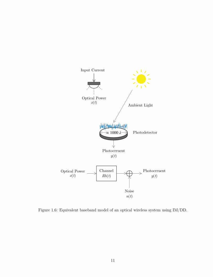
Figure 1.6: Equivalent baseband model of an optical wireless system using IM/DD.

11

DC gain for the receiver can be approximated by [10]:

Hlos(0) =

(m+1)A2πd2

cosm(ϕ) cos(ψ) 0 ≤ ψ ≤ Ψ1/2

0 ψ > Ψ1/2

(1.3)

where A denotes the photo-detector physical area, d denotes the distance be-

tween the receiver and the transmitter, ϕ denotes the irradiance angle with regard

to the transmitter perpendicular axis, ψ denotes the incidence angle with regard to

the perpendicular axis of the receiver, whereas Ψ1/2 denotes the FOV semi-angle

concentrator.

The Lambertian order m is expressed by:

m =− ln 2

ln(cos(Φ1/2))(1.4)

Where Φ1/2 represents the LED half-power angle; for instance, Φ1/2 = 60◦ corresponds

to m = 1.

The relation between the channel DC gain and the channel impulse response is

given by:

H(0) =

∫ +∞

−∞h(t)dt (1.5)

The optical power received Pr is expressed based on the transmitted power Pt and

the channel gain as shown:

Pr−los = H(0)losPt (1.6)

12

Figure 1.7: VLC downlink transmission geometry of a LOS path.

13

1.1.2 Path Loss Model

Within communication systems, path loss refers to the attenuation that electromag-

netic waves experience in transit between a receiver and a transmitter. Path loss could

be attributed to several effects that include absorption, aperture-media coupling loss,

reflection, refraction, and loss of free space. In most cases, dB constitutes the units for

expressing path loss. The channel’s linear path loss could be written as the transmit

power-receiver power ratio:

PL =Pt

Pr

=1

H(0)= (H(0))−1 (1.7)

Expressing path loss in dB, we obtain:

PLdB = 10 log10 (H(0))−1 = −10 log10 (H(0)) (1.8)

1.2 Underwater VLC Systems

Demand for underwater systems of communication are on the rise because of the

continuing human activity expansion in underwater settings, for instance, tactical

surveillance, port security, offshore oil explorations, maritime archeology, underwa-

ter scientific collection of data, and environmental tracking [12]. Three technologies

utilized for underwater communication exist namely optics, RF, and acoustics [13].

14

The acoustic technique constitutes the most extensively utilized technology within

UWC because it is capable of achieving a prolonged connection ranging up to many

kilometers [14]. Nevertheless, it is characterized by numerous technical pitfalls.

Firstly, acoustic connections have low rates of data (in Kbps) [15]. Secondly, acoustic

links are prone to serious communication delays (mainly in seconds) because of the low

propagation velocity of sound waves within water (around 1500m/s for pure water at

200C. Therefore, they might not be utilized for real-time exchange of data. Thirdly,

acoustic transceivers are often energy consuming, expensive and bulky [16].

RF waves could initiate smooth transition via water/air interfaces and have a

higher tolerance for water turbulence [13]. Nevertheless, the main drawback of under-

water RF communications is the short range of connection. The RF waves could solely

propagate a few meters in additional –low frequencies (30-300Hz) [15]. Besides, the

underwater RF systems necessitate energy-consuming, expensive, and bulky receivers

and transmitters.

Unlike RF and acoustic underwater techniques, underwater visible light commu-

nication (UVLC) is characterized by the lowest costs for implementing it, lowest con-

nection delay, highest security and highest rates of data transmission (in the sequence

of Gbps on moderate distances) [13].

Because water is transparent to green or blue light (450 nm – 550 nm), light emit-

ting diodes (LEDs) or visible light lasers could be utilized as transmitters of underwa-

ter wireless connectivity with rates of data in the sequence of 10 Mb/s. Experimental

UVLC demonstrations that surpass Gb/s were found within a regulated laboratory

setting [17]–[20]. The past few years have been characterized by increased literature

15

about VLC spanning from the modeling of channels to issues of the upper layer and

physical layer [21]–[34].

1.2.1 Path Loss Model

The UVLC path loss constitutes the geometrical loss and attenuation loss function.

The attenuation loss is identified through scattering and absorption. Absorption refers

to an energy transfer process wherein photons forego their energy and transform it

into other types, such as chemical or heat. Scattering is the light deflection from the

initial path because of interactions with transmission media atoms and molecules.

The Beer-Lambert formula [35] is extensively utilized within the literature for

computing underwater path loss.

PLBL(d) = 10 log10 e−cd (1.9)

where d represents the connection range between receivers and transmitters,

whereas c denotes the overall attenuation. The coefficient c could be denoted as

c = a + b, where a and b represent the scattering and absorption coefficients. The

Beer-Lambert principle rides on two assumptions that underestimate the optical power

received. Firstly, the receiver and transmitter have perfect alignment. Secondly, all

scattered photons become displaced even though some scattered photons could still

reach the receivers following several events of scattering.

Geometrical loss is caused by the dispersal of transmitted beams between the

receiver and the transmitter. In most cases, the beam disperses to sizes that are

16

larger than the aperture of the receiver, thus leading to the loss of the overfill energy.

Taking into account the line-of-sight (LOS) configuration alongside semi-collimated

laser sources with Gaussian beam-shapes, the geometrical loss could be estimated

as [36]:

PLGL(d) ≈ 10 log10

((DR

θ1/ed

)2)

(1.10)

where DR represents the diameter of the aperture receiver whereas θ1/e represents the

total width transmitter beam divergence angle1. Consistent with (1.9) and (1.10), the

total path loss is expressed by:

PL(d) = PLBL(d) + PLGL(d) (1.11)

≈ 10 log10

((DR

θ1/ed

)2

e−cd

)

Practically, the detector could receive rays following several multiple scattering

while the formulation above rides on the assumption that scattered rays are unavail-

able. To consider the impetus of scattered rays, an improved version for (1.11) is

suggested in [37]:

PL(d) ≈ 10 log10

((DR

θ1/ed

)2

e−cd

(DR

θ1/ed

)T)(1.12)

where another term that is proportional to light source geometrical propagation is

unveiled within the negative exponential. In equation (1.12), T represents a correction

coefficient that could be identified by fitting data to simulated data.

17

1.2.2 Turbulence Channel Model

Most existing literature regarding underwater optical wireless communications [22],

[30], [38], [39] take into account deterministic path loss models at the expense of

turbulence-induced fading. Underwater optical turbulence takes place because of the

seawater refractive index changes and unveils instantaneous reductions on the mean

received power [13]. Ocean currents are the common cause of such a phenomenon that

induces sudden differences in water pressure and temperature.

The underwater optical turbulence (UOT) model was borrowed from the classical

log-normal turbulence model utilized within free-space optical (FSO) communication

[40]:

fI(I) =1√

2πσtIexp

(−(ln I − µ)2

2σ2t

), I > 0 (1.13)

where fI(I) denotes the UOT PDF, I represents the obtained optical irradiance,

µ represents the average logarithmic light density whereas σ2t denotes the index of

scintillation.

1.3 Modulation Techniques

Notably, four modulation schemes that are utilized in VLC communication exist;

they include Color Shift Keying (CSK), Orthogonal Frequency Division Modulation

(OFDM), Pulse Modulation Methods, and On-Off Keying (OOK). In [41], the per-

formance for such schemes is evaluated based on power requirements, Bit Error Rate

(BER), Signal to Noise Ratio (SNR) and data rate.

18

1.3.1 On-Off Keying (OOK)

Within the scheme, the source of light is switched on during transmission of logic 1 and

is switched off during logic 0 transmission. In off state, the light intensity is reduced

(not totally switched off). Fig. 1.8 illustrates the string of data “101101” with OOK-

RZ (Return-to-Zero) and OOK-NRZ (Non-Return-to-Zero) modulation schemes. The

OOK scheme provides appropriate characteristics, for instance, simple implementa-

tion. Nevertheless, the major OOK restriction is the lower rates of data, particularly

in the maintenance of various levels of dimming.

1.3.2 Pulse Modulation Methods

Within the schemes, pulse position and pulse width represents the conveyed data. In

Pulse Width Modulation (PWM) scheme, the conveyed signal undergoes modulation

through digital pulses, whereby pulses that correspond to logic 1 possess varying width

as opposed to those denoting logic 0. Within Pulse Position Modulation (PPM), the

pulses width remains unchanged while each pulse’s position is varied on the basis of the

logical values earmarked for transmission. The Variable Pulse Position Modulation

(VPPM) constitutes the PWM and PPM consolidation where pulse position and width

undergo variation. Fig.1.9 presents a schematic diagram that shows the variation

between VPPM, PPM, and PWM. Other pulse modulation method variations are

explored in [41]. The major benefit of pulse modulation schemes is the capacity

of achieving the needed level of dimming without using color shifts on the ejected

light [42]. Nevertheless, such schemes are generally characterized by low rates of data.

19

Figure 1.8: Representation of the data string “101101” using OOK-NRZ and OOK-RZmodulation schemes.

20

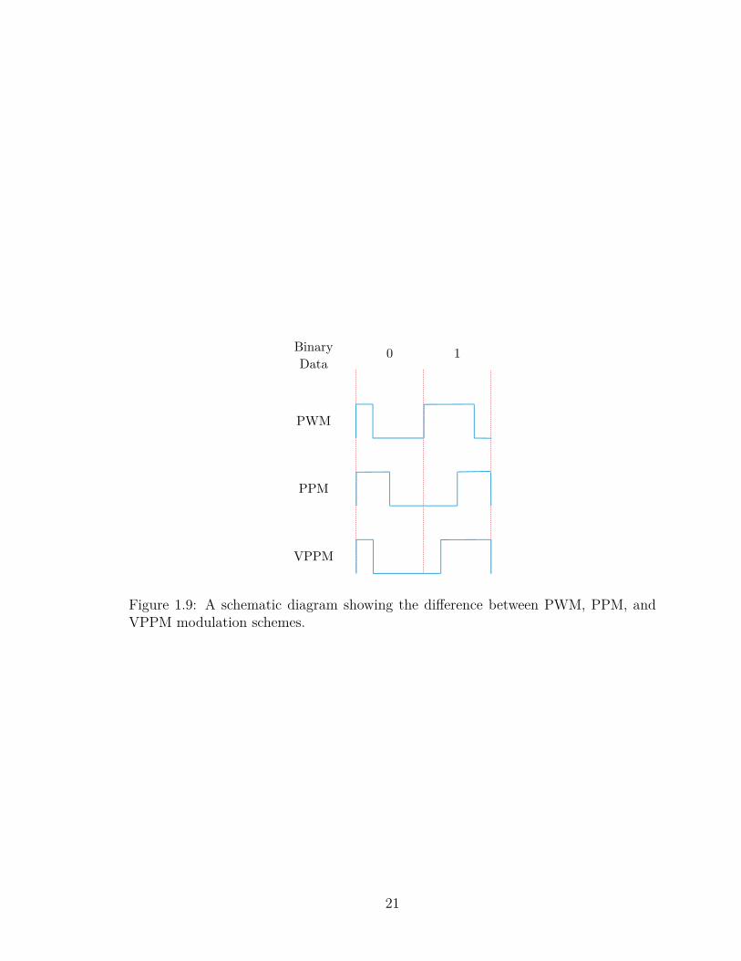
Figure 1.9: A schematic diagram showing the difference between PWM, PPM, andVPPM modulation schemes.

21

1.3.3 Orthogonal Frequency Division Multiplexing (OFDM)

Past modulation schemes are categorized as single-carrier modulation schemes. Single

carriers are marred by high Inter-symbol interference (ISI) wherein a single symbol

interrupts subsequent symbols because of nonlinearity within the VLC channels fre-

quency response [41]. OFDM constitutes a frequency-division multiplexing (FDM)

scheme utilized as the digital multicarrier modulation technique. The transmitter uti-

lizes modulation methods that include QAM or QPSK to expand OFDM symbol’s

data capacity. For instance, a 16-QAM modulation maps 4 data bits to complex

symbols. The complex symbols are transported by one OFDM symbol subcarrier.

Afterward, several subcarriers are conveyed with each transporting various data sym-

bols to expand the rate of data. Fig.1.10 illustrates this process. The three major

challenges to OFDM within the VLC system include its restricted dimming support,

the higher peak-to-average power ratio (PAPR) and the LED’s nonlinearity, that is,

the correlation between the LED emitted light and current is not linear. Despite such

challenges, OFDM has a huge potential within VLC communication because of its

immunity to inter-symbol interference and a high rate of data [41]. The basic OFDM

block diagram is illustrated within Fig.1.11 wherein fast Fourier transform (FFT) is

utilized at the receivers and inverse fast Fourier transform (IFFT) is utilized at OFDM

transmitters.

22

Figure 1.10: Illustration of the OFDM transmission.

23

Figure 1.11: Basic OFDM System.

24

1.3.4 Color Shift Keying (CSK)

To address challenges emanating from other modulation schemes (for instance, re-

stricted dimming support and low rate of data, IEEE 802.15.7 standard recommended

CSK modulation which is developed mainly for VLC [43]. The block diagram for a

basic CSK system is illustrated in Fig.1.12. The CSK scheme modulates the signal

through the three color (blue, green, and red) intensity that tri-color LEDs (TLED)

generated. The premise of the modulation is on the color space chromaticity diagram

that CIE 1931 described and which is illustrated within Fig.1.13. Within CSK mod-

ulation, the bit patterns undergo encoding to wavelength (color) combinations. For

instance, within the 8-CSK (refer to Fig.1.14), the source of light undergoes wave-

length keying such that one out of 8 potential colors (wavelengths) is transmitted for

each combined bit pair.

1.4 Multiple Access

Multiple access (MA) is utilized within VLC to grant simultaneous access to network

services or resources for multiple users. Multiple accesses could be attained through

three potential topologies presented within Fig.1.15 namely cellular topology with

several APs shared by multiple users, single-cell topology with one AP for each room,

and single –cell topology with one AP for each user [44]. An ideal topology is selected

on the basis of network services, users’ mobility, user number, and room size. The

initial topology is feasible for users in buses, trains, or airplanes where there is one lamp

(AP) on top of every seat. One cell per-room topology could be utilized in moderating

25

Figure 1.12: Basic TLED CSK System.

26

Figure 1.13: CIE 1931 color space chromaticity diagram.

27

Figure 1.14: Symbol mapping for 8-CSK.

28

the size of offices or rooms. Cellular topologies are needed to cover airport terminals

or big halls.

Numerous MA methods including non-orthogonal multiple access (NOMA), or-

thogonal frequency domain multiple access (OFDMA), space division multiple access

(SDMA), wavelength division multiple access (WDMA), code division multiple ac-

cess (CDMA), frequency division multiple access (FDMA), and time division multiple

access (TDMA), have been suggested for VLC [44].

In this dissertation, we propose a new resource allocation model based on a well-

known video game called the Tetris game. We have used metaheuristic algorithm such

as simulated annealing (SA) simulated evolution (SimE) to optimize the RA with the

objective of maximizing the system data rate under the considered partial fairness.

Our Tetris model has three main contributions:

1. Reducing the time complexity of computing the cost function fromO(T×N×M)

to O(T ) which has a significant impact on the running time of the optimization

algorithms.

2. Improving the convergence of the optimization algorithms by considering fixed

block assignments (Tetris pieces in our model) of users with the optimal data

rate instead of individual slot assignments.

3. Handling the fairness objective independently from the allocation process by

increasing the number of time slots assigned to users with low data rates when

creating block assignments (Tetris pieces).

The rest of this dissertation is organized as follows. Chapter 2 reviews literature

29

Figure 1.15: Multiple access topologies for VLC: (a) single AP per-user; (b) single APper-room; and (c) cellular topology using multiple APs.

30

in the area of VLC and presents research objectives. Chapter 3 presents our Tetris-

Game model to solve the resource allocation problem. The implementation details of

the proposed optimization heuristics are discussed in Chapter 4. Chapter 5 discusses

the experimental results of the proposed optimization heuristics.

31

CHAPTER 2

PROBLEM DEFINITION AND

RESEARCH OBJECTIVES

In this chapter, we formulate the VLC resource allocation problem and present the

research objectives. We start by a literature review of active research areas in the

field of VLC systems. Then, we introduce the considered resource allocation problem

and give its formal description as an optimization problem. After that, we discuss the

motivation behind the selected problem. Finally, we present our research objectives.

2.1 Literature Review

As the revolutionary remedy to wireless communications containing different potential

areas of application, the VLC technology has attracted the attention of investigators

on a variety of levels. While studies on the physical layers are crucial in facilitating the

technology, there is a need for extensive efforts within the top layers to change VLC

into fully-functioning, scalable, and multi-user wireless networking technology. From

32

this perspective, several studies on resource allocation, load balancing, and handover

were cited within the literature.

2.1.1 Handover

Handover schemes are utilized for transferring the management of a wireless trans-

mission session that is underway from a single AP towards another. In most cases,

Handover is needed within two cases [4]. Firstly, a mobile terminal exits one AP

coverage area and enters another AP coverage area. Secondly, the channel of trans-

mission is reduced because of interference or overloading. Classification of handover

could be undertaken on the basis of the number of networks featured in two forms

namely, vertical handover and horizontal handover [45]. Horizontal handover occurs

between APs in one network. Vertical handover occurs between different network

APs. Horizontal handover could be divided further into two forms based on the si-

multaneous connections’ quantity: soft handover and hard handover [45]. In hard

handover, mobile terminals could be served solely by a single AP at a given duration.

Therefore, it would be delinked from the present AP prior to its connection to the

following AP triggering a connectivity disruption. The key benefit of this kind is the

lower complexity of the hardware and simpler implementation. Within soft handover,

the mobile terminal could be served using multiple AP simultaneously. Therefore, the

connection of the terminal to the existing AP is not terminated until the connection

to the following AP is successful. This type provides ideal user experiences; however,

it necessitates sophisticated implementation and more resources.

33

A number of handover schemes for VLC have been proposed over the past few

years. The techniques in [46], [47] extend the traditional RSS-based handover proce-

dures for mobile VLC systems. The work in [48], proposes a hybrid VLC and OFDMA

network model in which the VLC channel is used for downlink transmission, while

OFDMA channels are only used for uplinks and downlinks if there is no coverage of

VLC hotspots. The proposed system combines horizontal and vertical mobile termi-

nal handover methods to manage the mobility of users between different hotspots and

OFDMA systems. In [49], soft handovers based on power and frequency are proposed

to reduce data rate variations as the mobile terminal moves from cell to the other.

In [50], a handover scheme combined with the joint transmission is proposed for VLC

networks. The proposed scheme is compared against the data rates and the SINR of

a hard-handover scheme.

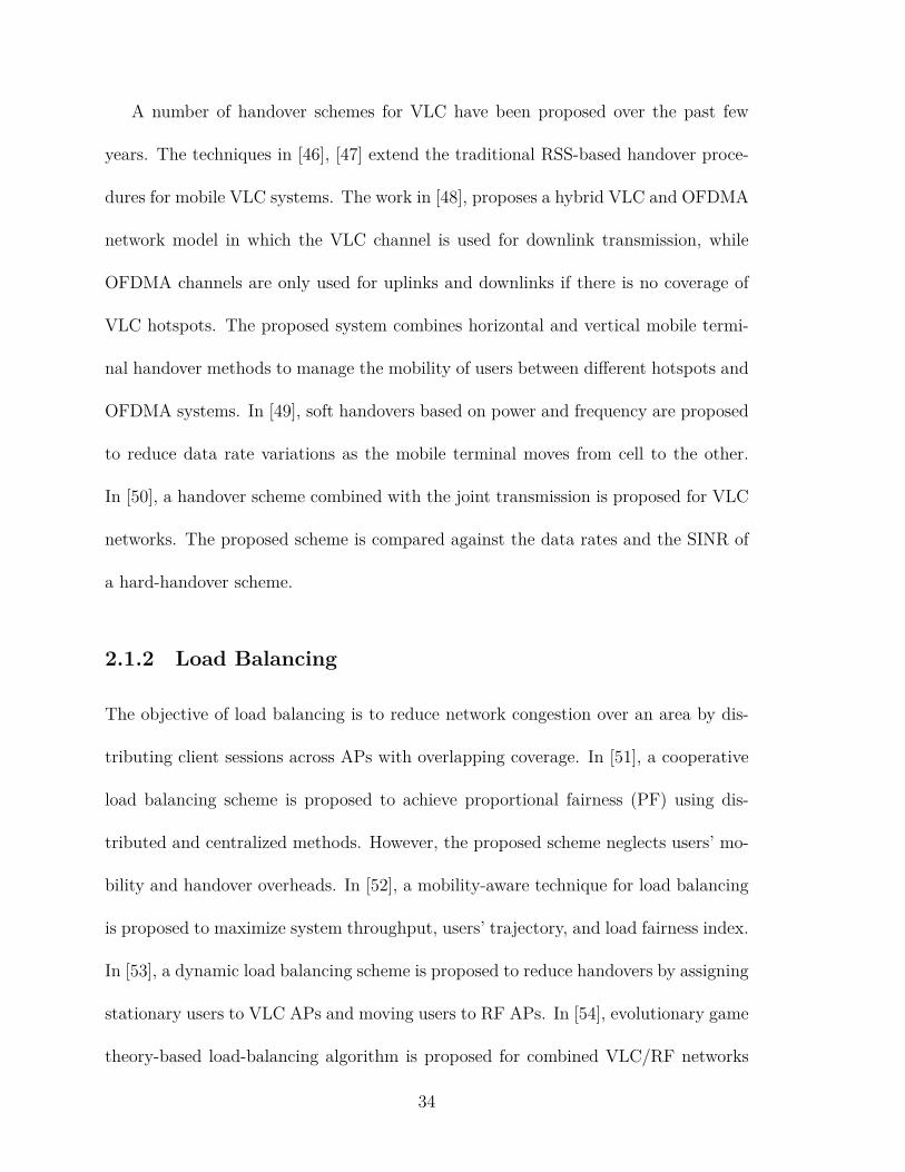
2.1.2 Load Balancing

The objective of load balancing is to reduce network congestion over an area by dis-

tributing client sessions across APs with overlapping coverage. In [51], a cooperative

load balancing scheme is proposed to achieve proportional fairness (PF) using dis-

tributed and centralized methods. However, the proposed scheme neglects users’ mo-

bility and handover overheads. In [52], a mobility-aware technique for load balancing

is proposed to maximize system throughput, users’ trajectory, and load fairness index.

In [53], a dynamic load balancing scheme is proposed to reduce handovers by assigning

stationary users to VLC APs and moving users to RF APs. In [54], evolutionary game

theory-based load-balancing algorithm is proposed for combined VLC/RF networks

34

with shadowing and blocking. The work in [55] suggests a combination of load bal-

ancing and power allocation schemes for hybrid RF and VLC networks. The scheme

distributes users on APs and distributes the powers of the APs on their assigned users

using an iterative algorithm. The experimental results show an improved system

capacity fairness with fast convergence.

2.1.3 Resource Allocation

VLC network resources such as time, power, spectrum and data rates are limited and

distributed among multiple users. This limitation creates a number of problems in

the allocation of resources that are interesting from both application and theoretical

levels.

The work in [56] investigates a decentralized interference management scheme for

OFDMA VLC system deployed inside an aircraft. In this scheme, each user equip-

ment (UE) must transmit a busy burst (BB) in a time-multiplexed slot after receiving

data successfully in order to reserve the time-frequency slot for the following frame.

The access point (AP) planning to send data on a given slot must listen to its corre-

sponding BB to decide whether to transmit or delay the transmission to another slot

without any centralized controller in order to limit the interference of the co-channel.

In [57], a centralized resource allocation scheme is proposed to assign the visible light

multi-color logical channels to different users to minimize the interference between

co-channel. A resource allocation system for VLC systems based on locations is in-

troduced in [58]. The scheme uses a proportional fair (PF) scheduling algorithm to

accommodate various transmission scenarios. In [59], a scheduling scheme is proposed

35

to assign LED lamps to multiple users for indoor VLC systems with the aim of mini-

mizing inter-user interference. The authors presented a weighted graph to model the

interference between users and solved the problem using a deterministic algorithm.

In [60], the problem of resource allocation (RA) of moving terminals is studied on

the basis of various transmission approaches to achieve relative fairness under delay

conditions. The RA problem is then constructed as a non - linear programming prob-

lem (NLP) and solved through convex optimization methods. The centralized scheme

proposed in [61] covers both the load balancing and the allocation of resources for the

OFDM VLC system. The scheme uses a fuzzy logic algorithm to allocate resources

and select an appropriate AP. A beam allocation scheme for the elimination of co-

channel interference in VLC networks is proposed in [62]. In [63], a dynamic resource

allocation scheme for hybrid VLC – radio frequency (RF) networks is proposed. The

problem of resource optimization is implemented using the Lyapunov optimization

technique. In [64], the allocation of downlink channel resources in VLC networks is

studied. In [65], a resource allocation algorithm for down-link VLC networks is pro-

posed. The problem is represented as a mixed-integer binary problem, and is solved

by a centralized coordinator using Cuckoo search algorithm. An interference-free al-

location system for LEDs is investigated in [66]. The work in [50] proposed a mobility

management and resource allocation algorithm for VLC networks. The problem is

formulated as a nonlinear integer programming problem, and is solved by means of a

particle swarm optimization (PSO) algorithm.

36

2.2 Dynamic LED Allocation Problem

In this section, we present the dynamic LED allocation problem in visible light com-

munication systems for both indoor and underwater scenarios. For both scenarios, we

will assume a centralized light access network (C-LiAN), where all light access points

are controlled by a central control unit. We will describe the setup of the considered

systems in indoor and underwater environments.

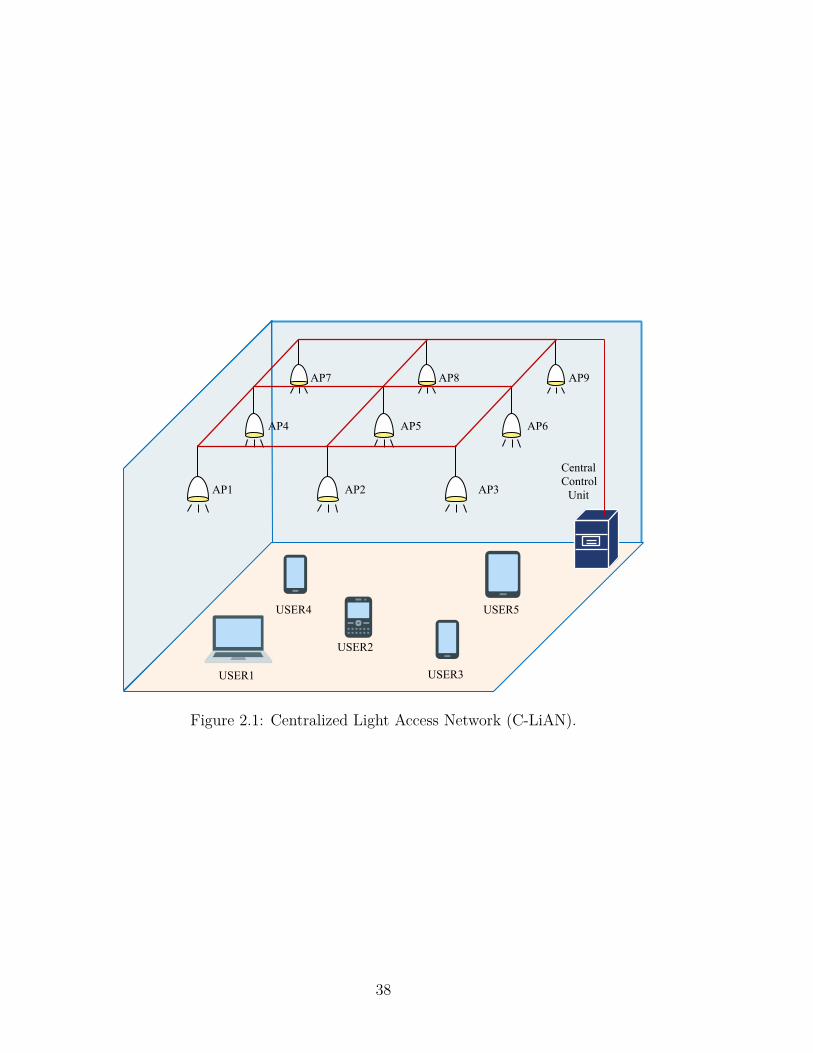
2.2.1 LED Allocation for Indoor C-LiAN

In this dissertation, we consider a centralized light access network (C-LiAN) [67] with

N LEDs, as illustrated in Fig. 2.1, and assume a multi-user environment with M

users. A centralized unit manages the LEDs and handles the the allocation of the

LED resources to users.

The transmitted signal sn(t) from the nth LED is carried on a background DC

light intensity with average power Pavg which is commonly used for light illumination.

The signal sn(t) has zero mean and a variance of Pn which is the power of the LED

as illustrated in Fig. 2.2 [68]. The standard deviation of the signal sn(t) is√Pn.

37

Central

Control

UnitAP1 AP2 AP3

AP4 AP5 AP6

AP7 AP8 AP9

USER1

USER2

USER3

USER4 USER5

Figure 2.1: Centralized Light Access Network (C-LiAN).

38

Figure 2.2: Conceptual illustration for the background DC level and communicationsignal on the nth LED.

39

The received signal at the uth user can be written as:

yu = R

N∑n=1

√Pnαn,uHn,uxu +R

N∑n=1

M∑m=1m̸=u

√Pnαn,mHn,uxm + wu (2.1)

where xu is the transmitted signal to the uth user, R denotes the optical to electrical

conversion coefficient, Pn is the transmission power of the nth LED, Hn,u is the chan-

nel response from the nth LED to the uth user, and wu denotes the Additive White

Gaussian Noise (AWGN) with zero-mean and σ2 variance at the uth user side. The

connectivity variable αn,u is equal to 1 when the nth LED is assigned to uth user, and

is equal to 0 otherwise. The first term denotes transmitted signal from LEDs assigned

to the uth and the second term is the interference from the other LEDs.

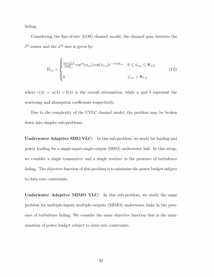
Considering the line-of-site (LOS) channel model, the channel gain between the

ith AP and the uth user is given by [10]:

Hi,u =

(m+1)A

2πd2i,ucosm(ϕi,u) cos(ψi,u) 0 ≤ ψi,u ≤ Ψ1/2

0 ψi,u > Ψ1/2

(2.2)

where A denotes the photo-detector physical area, di,u denotes the distance between

the receiver and the transmitter, ϕi,u denotes the irradiance angle with regard to

the transmitter perpendicular axis, ψi,u denotes the incidence angle with regard to

the perpendicular axis of the receiver, whereas Ψ1/2 denotes the FOV semi-angle

concentrator. The Lambertian order m is expressed as: m = −1/ log2(cos(Φ1/2)),

where Φ1/2 is the half-power angle of the LED. For example, Φ1/2 = 60◦ corresponds

40

to m = 1.

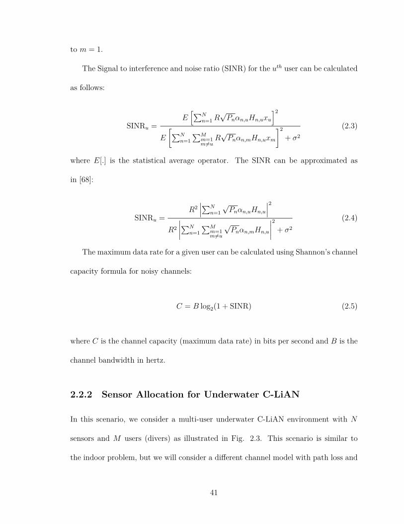
The Signal to interference and noise ratio (SINR) for the uth user can be calculated

as follows:

SINRu =E[∑N

n=1R√Pnαn,uHn,uxu

]2E

[∑Nn=1

∑Mm=1m̸=u

R√Pnαn,mHn,uxm

]2+ σ2

(2.3)

where E[.] is the statistical average operator. The SINR can be approximated as

in [68]:

SINRu =R2∣∣∣∑N

n=1

√Pnαn,uHn,u

∣∣∣2R2

∣∣∣∣∑Nn=1

∑Mm=1m̸=u

√Pnαn,mHn,u

∣∣∣∣2 + σ2

(2.4)

The maximum data rate for a given user can be calculated using Shannon’s channel

capacity formula for noisy channels:

C = B log2(1 + SINR) (2.5)

where C is the channel capacity (maximum data rate) in bits per second and B is the

channel bandwidth in hertz.

2.2.2 Sensor Allocation for Underwater C-LiAN

In this scenario, we consider a multi-user underwater C-LiAN environment with N

sensors and M users (divers) as illustrated in Fig. 2.3. This scenario is similar to

the indoor problem, but we will consider a different channel model with path loss and

41

fading.

Considering the line-of-site (LOS) channel model, the channel gain between the

ith sensor and the uth user is given by:

Hi,u =

(m+1)A

2πd2i,ucosm(ϕi,u) cos(ψi,u)e

−c(λ)di,u 0 ≤ ψi,u ≤ Ψ1/2

0 ψi,u > Ψ1/2

(2.6)

where c(λ) = a(λ) + b(λ) is the overall attenuation, while a and b represent the

scattering and absorption coefficients respectively.

Due to the complexity of the UVLC channel model, the problem may be broken

down into simpler sub-problems.

Underwater Adaptive SISO VLC: In this sub-problem, we study bit loading and

power loading for a single-input-single-output (SISO) underwater link. In this setup,

we consider a single transmitter and a single receiver in the presence of turbulence

fading. The objective function of this problem is to minimize the power budget subject

to data rate constraints.

Underwater Adaptive MIMO VLC: In this sub-problem, we study the same

problem for multiple-inputs multiple-outputs (MIMO) underwater links in the pres-

ence of turbulence fading. We consider the same objective function that is the mini-

mization of power budget subject to data rate constraints.

42

Figure 2.3: A multi-user underwater C-LiAN environment.

43

2.3 Problem Definition

As indicated in the previous section, we consider a centralized light access network

(C-LiAN) environment with N LEDs and M users. Each LED uses the same spec-

trum and time-division multiple access (TDMA) is assumed in downlink transmission.

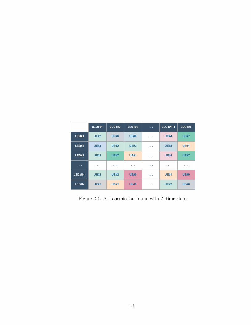
One transmission frame includes T time slots as illustrated in Fig. 2.4. Hence, the

maximum allowed serving user count is equal to T ×N because one user is allocated

only one LED and only one-time slot. However, based on the total number of users,

multiple LEDs can be allocated to a single user within the same time slot, which is

also called “Coordinated Multi-point Transmission.”

Next, we formulate the allocation problem as an optimization problem by defining

the three optimization elements: decision variables, constraints, and objective func-

tions.

Decision Variables: We define a time-varying allocation matrix, A[t], as our deci-

sion variable. Each element αn,u[t] of A[t] takes a value of 0 or 1, where αn,u[t] = 1

indicates that the nth LED is assigned to the uth user in the tth time slot.

Constrains: In this problem, we consider two constraints:

1. Since the time-slot of an LED cannot be shared with multiple users, the following

equation should be satisfied while optimizing the allocation matrix:

M∑u=1

αn,u[t] ≤ 1; 1 ≤ n ≤ N, 1 ≤ t ≤ T (2.7)

44

SLOT#1 SLOT#2 SLOT#3 . . . SLOT#T-1 SLOT#T

LED#1 UE#2 UE#6 UE#8 . . . UE#4 UE#7

LED#2 UE#3 UE#2 UE#2 . . . UE#8 UE#1

LED#3 UE#2 UE#7 UE#1 . . . UE#4 UE#7

. . . . . . . . . . . . . . . . . . . . .

LED#N-1 UE#2 UE#2 UE#9 . . . UE#1 UE#9

LED#N UE#5 UE#1 UE#9 . . . UE#2 UE#6

Figure 2.4: A transmission frame with T time slots.

45

2. In order to serve a user by at least one LED within at least one time-slot, the

following equation should be satisfied:

N∑n=1

T∑t=1

αn,u[t] ≥ 1; 1 ≤ u ≤M (2.8)

The above constraints are valid under the assumption that the maximum T × N

users exist in the indoor room environment under consideration.

Objective Functions: In this problem, we consider the objective function of max-

imizing the system data rate under the consideration of partial fairness using the

following equation:

maxA[t]

(M∑u=1

T∑t=1

log2 (1 + SINRu[t])

)(2.9)

2.4 Motivation

Visible light communication (VLC) is a growing technology that can overcome the

limitations of the RF spectrum for wireless communication systems. VLC systems

have many advantages over RF-based communication systems such as broad-spectrum,

safety, low cost, energy efficiency, and information security. As a revolutionary solution

to wireless communications with a wide range of applications, the VLC technology

has attracted researchers on various levels such as the physical layer, handover, load

balancing, and resource allocation. While research on the physical layer is essential in

enabling this technology, more efforts are needed in the upper layer to transform VLC

into a multi-user, scalable, and fully functioning wireless networking technology. In

46

this context, we have chosen to contribute to this evolving research area concentrating

on the optimization problems of resource allocation.

2.5 Research Objectives

The allocation of resources in VLC systems is an attractive research area. Most of the

proposed schemes use deterministic algorithms to solve NP-hard allocation problems.

Our primary research objective is to explore the application of meta-heuristics for

optimizing a load-aware dynamic LED allocation system in C-LiAN. The potential

optimization problem to be pursued during the research is the maximization of system

data rate under the considered partial fairness. In addition to that, we will study a

similar problem to assign sensors to divers in underwater C-LiAN dynamically.

47

CHAPTER 3

THE TETRIS GAME MODEL

In this dissertation, we consider a resource allocation problem (RA) for an indoor room

environment with N LEDs and a multi-user environment with M users. A centralized

unit manages the LEDs and handles allocation of the LED resources to users. Each

LED uses the same spectrum and TDMA is assumed in downlink transmission. One

transmission frame includes T time-slots. Hence, maximum allowed serving user count

is equal to T × N considering the fact that one user is allocated with only one LED

and only one-time slot. However, based on the total number of users, multiple LEDs

can be allocated to a single user within the same time slot, which is also called as

“Coordinated Multipoint Transmission”. We have modeled this problem as a Tetris

game and used simulated annealing (SA) to optimize the RA with the objective of

maximizing system data rate under the considered partial fairness. Our Tetris model

has the advantage of improving the convergence of the optimization algorithms by

considering various block assignments (Tetris pieces in our model) instead of individual

slot assignments.

48

3.1 The Tetris Game

Tetris is a video game developed by Alexey Pajitnov in 1984. The game is played on a

board composed of R rows and C columns, in which pieces of 7 different shapes drop

from top to bottom as shown in Fig. 3.1. The optimization of the offline version of

the Tetris game is proven to be NP-complete [69]. The optimization objectives of this

problem include: maximizing the number of canceled rows, maximizing the number

of packed pieces, and minimizing the number of rows occupied by pieces.

Example 1. In this example, we illustrate the mapping between the RA problem

and the Tetris problem. Consider a room with four LEDs (N = 4) and four users

(M = 4); and assume that the channel gains are given by Table 3.1. Further, assume

that each transmission frame includes four time-slots (T = 4). A total of 16 time-slots

will be equally divided between the four users (4 time-slots per user). Table 3.2 shows

all possible LED allocations for each user with allocated LEDs hightailed in color. The

assignments are sorted in descending order of their data rates which are calculated

using equation (2.5). In our Tetris model, each user’s assignment represents a piece

consisting of LEDs assigned to that user with a weight corresponding to its data rate.

Finding the assignment that maximizes the overall data rate is equivalent to finding

an optimal packing of the pieces in a fixed height Tetris board such that the total

weight is maximized. Note that in order to satisfy the constraint in equation (2.8),

we need to pack at least one piece for each user in the Tetris board. Fig 3.2 shows an

optimal packing of the Tetris pieces from Table 3.2 in four rows (i.e., four time-slots).

The packing includes one piece with 4 LEDs for each one of the 1st and 3rd users, and

49

Board Pieces

Figure 3.1: An example of Tetris board with seven pieces (shapes).

50

two pieces with 2 LEDs for each one of the 2nd and 4th users.

3.2 The Tetris Model

Given an instance of the RA problem with N LEDs, M users, T time-slots, one can

map this problem into a Tetris game with p pieces and an m×n board, where n = N

and T ≤ m ≤ p. The model uses two structures: one to store the pieces (allocation

combinations) and the other to store the pieces packed in the Tetris board (allocation

solution).

3.2.1 Tetris Pieces

The Tetris pieces can be represented as an array Tetris of p elements (structures).

Each element Tetris[k] represents one piece in the Tetris game model which contains

the following members:

• Piece (pk): an n−tuple of the form (a1, a2, . . . , an) which represents an allocation

to a user uk, where ai = 1 if the ith LED is allocated for the user and 0 otherwise.

• User (uk): the user associated with the piece pk.

Fig. 3.3 shows the array Tetris representing the pieces in Table 3.2.

3.2.2 Solution Representation

In a direct implementation of the RA problem, a solution S can be represented as

N × T matrix where the element S[i, j] = u indicates that the ith LED is assigned to

51

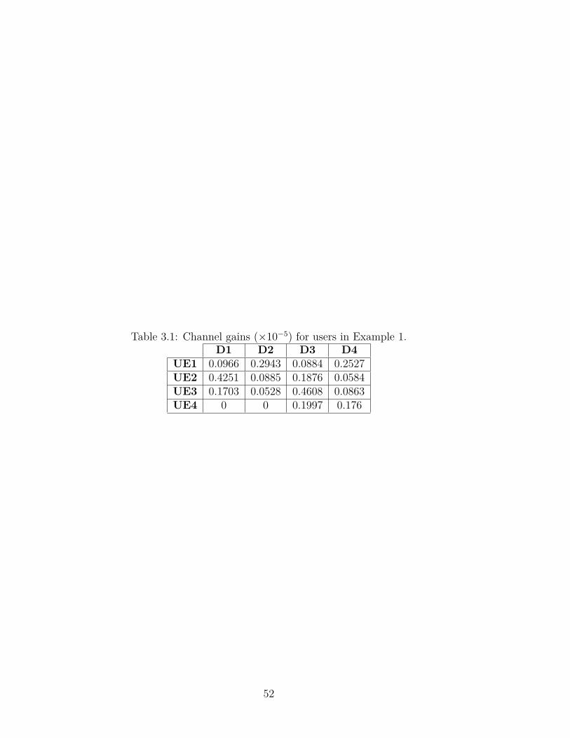
Table 3.1: Channel gains (×10−5) for users in Example 1.D1 D2 D3 D4

UE1 0.0966 0.2943 0.0884 0.2527UE2 0.4251 0.0885 0.1876 0.0584UE3 0.1703 0.0528 0.4608 0.0863UE4 0 0 0.1997 0.176

52

Table 3.2: All possible combinations of Tetris pieces for users in Example 1.UE # D1 D2 D3 D4 D. Rate UE # D1 D2 D3 D4 D. Rate

1 1 1 1 1 9.716115 31 1 1 1 1 9.8627822 1 1 0 1 5.644801 32 1 0 1 1 7.2425353 0 1 1 1 5.375191 33 1 1 1 0 5.8773014 0 1 0 1 3.260951 34 1 0 1 0 4.3871595 1 1 1 0 2.189977 35 0 1 1 1 3.7168336 1 0 1 1 1.675555 36 0 0 1 1 2.7955967 1 1 0 0 1.205903 37 0 1 1 0 2.3124968 0 1 1 0 1.133929 38 0 0 1 0 1.6799419 1 0 0 1 0.871187 39 1 1 0 1 0.53539310 0 0 1 1 0.813839 40 1 0 0 1 0.32081211 0 1 0 0 0.536918 41 1 1 0 0 0.22129212 0 0 0 1 0.352892 42 1 0 0 0 0.11156513 1 0 1 0 0.155868 43 0 1 0 1 0.06833914 1 0 0 0 0.032908 44 0 0 0 1 0.022788

1

15 0 0 1 0 0.026907

3

45 0 1 0 0 0.007772

UE # D1 D2 D3 D4 D. Rate UE # D1 D2 D3 D4 D. Rate16 1 1 1 1 9.823388 46 0 0 1 1 7.79645317 1 1 1 0 6.934416 47 0 0 1 0 1.17768718 1 0 1 1 5.759876

448 0 0 0 1 0.818933

19 1 0 1 0 4.16100120 1 1 0 1 3.34080221 1 1 0 0 2.4091722 1 0 0 1 2.01494623 1 0 0 0 1.38155524 0 1 1 1 0.6934625 0 1 1 0 0.40616126 0 0 1 1 0.29743427 0 0 1 0 0.14711328 0 1 0 1 0.0805429 0 1 0 0 0.024832

2

30 0 0 0 1 0.009974

53

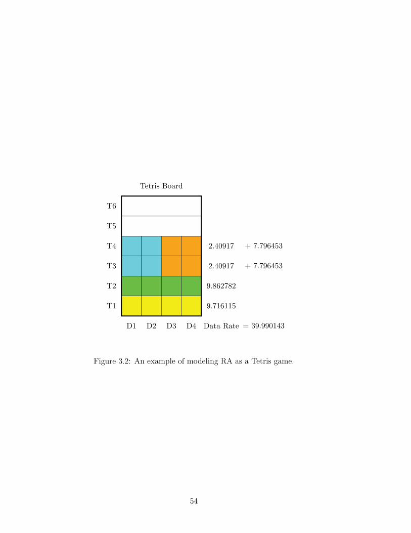
Figure 3.2: An example of modeling RA as a Tetris game.

54

Figure 3.3: Representation of the pieces in Table 3.2.

55

the uth user in the jth time slot. Table 3.3 shows the representation of the solution in

Fig. 3.4.

A solution of the RA problem modeled as a Tetris game can be represented as an

array S of m elements (structures), where T ≤ m ≤ p. The element S[r] represents the

assignment to the rth row of the Tetris board and it contains the following members:

• Assignment (Ar): an n−tuple of the form (a1, a2, . . . , an) combining (ORing)

the pieces placed in to the rth row.

• Pieces (Pr): a list of pieces placed in to the rth row.

Fig. 3.4 illustrates the solution representation of the assignment in Example 1 (see Fig

3.2). Each solution S is associated with a weight (Ws) proportional to the total data

rate of the pieces placed in to rows (time-slots) from 1 to T . This weight is calculated

as follows:

Cs = BM∑u=1

T∑t=1

log2 (1 + SINRu[t]) (3.1)

Ws = CsM

′

M(3.2)

where Cs is the total data rate of S, M is the total number of users, and M′ is the

total number of users with allocated time-slots between 1 and T . Note that the ratio

M′/M is used to penalize solutions violating the constraint in equation (2.8).

56

Table 3.3: A representation of the solution in Example 1 using a direct implementation.T#1 T#2 T#3 T#4

LED#1 1 3 2 2LED#2 1 3 2 2LED#3 1 3 4 4LED#4 1 3 4 4

57

Figure 3.4: A solution representation of the assignment in Example 1.

58

3.2.3 Extended Solution Representation

As discussed in section 3.2.2, we have two representations of the RA solution: one

for the direct implementation and one for the Tetris-Game model. In the direct

implementation, there exists a total of N × T slots that can be allocated to M users.

If the slots are equally divided between users, then each user will have (N × T )/M

slots. Since the objective is to maximize the system data rate under the consideration

of partial fairness, some users may be allocated more slots than others as long as the

constraint in equation (2.8) is respected. Therefore, we decided to use K×T time-slots

instead of T time-slots as defined in the original problem, where K is an integer greater

than 1. This allows the initial solution generator to include extra assignments for each

user (K×N×T )/M . Then, it is up to the optimization algorithm to allocate the slots

to maximize the total data rate in the first T time-slots. Note that the assignments in

the remaining (K × T − T ) time-slots are not included in the calculation of the total

data rate, hence, they should be occupied by assignments with the least data rates.

The extended solution representation for direct implementation of the RA problem is

illustrated by an example in Fig. 3.5.

In the Tetris-Game model, the extension of the solution is done in a different

manner. Instead of using extra time-slots, we repeat each generated piece K times,

where K is an integer that can be selected based on experimental results. Then, the

optimization algorithm will try to pack the pieces into T rows of the Tetris board such

that the total data rate is maximized. The remaining pieces placed into rows grater

than T will not participate in the calculation of the total data rate.

59

Figure 3.5: An example of the proposed extended solution representation.

60

3.3 Generating Tetris Pieces

Our experiments show that metaheuristic algorithms converge faster when using the

Tetris model allocation as compared to the individual LED allocation. However,

generating all possible combinations of the pieces is intractable for practical problems.

This makes individual allocation more flexible in exploring the various assignment

combinations. In order to take advantage of both approaches, we use large pieces

with high weights and small pieces (single LED assignments) with low weights. The

large pieces speed up the search process, while small pieces enable the optimization

algorithm to explore more areas by merging individual assignments to form pieces

with new combinations. In Example 1, we can generate the assignment of the 2nd user

in T3 using either a single piece with (1, 1, 0, 0) or using two pieces with (1, 0, 0, 0)

and (0, 1, 0, 0) respectively.

When generating the pieces for each user, we consider only LEDs with nonzero

channel-gain. In our Tetris model, we generate two sets of pieces for each user:

1. Single LED Allocation: consists of all combinations of pieces with a single

LED allocation. In Example 1, the first three users have four possible pieces

{(1, 0, 0, 0), (0, 1, 0, 0), (0, 0, 1, 0), (0, 0, 0, 1)}, while the last user has only two

possible pieces {(0, 0, 1, 0), (0, 0, 0, 1)}.

2. Multiple LEDs Allocation: consists of pieces with group of (2, 3, . . . , N) LEDs

selected based on their channel-gains ordered from highest to lowest. In Example

1, the first user has the following channel-gains (0.0966, 0.2943, 0.0884, 0.2527),

and his set of group allocations is given by {(0, 1, 0, 1), (1, 1, 0, 1), (1, 1, 1, 1)}.

61

Algorithm 1 shows how to generate the two sets of pieces for each user.

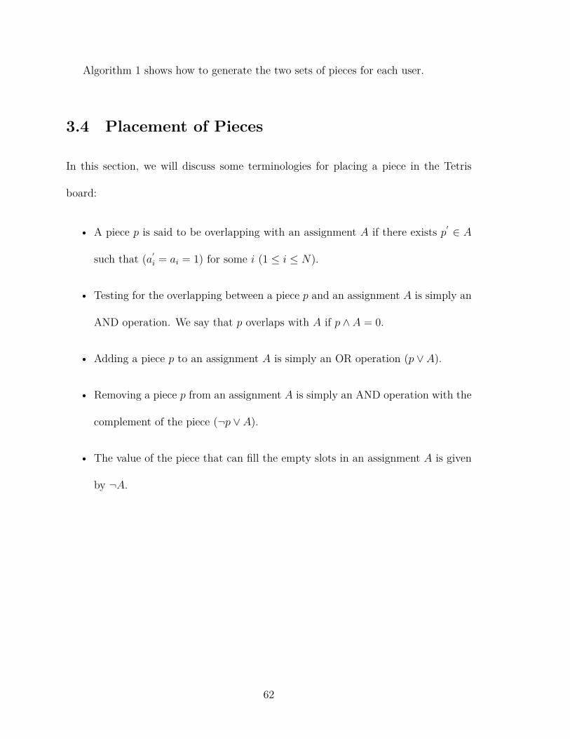
3.4 Placement of Pieces

In this section, we will discuss some terminologies for placing a piece in the Tetris

board:

• A piece p is said to be overlapping with an assignment A if there exists p′ ∈ A

such that (a′i = ai = 1) for some i (1 ≤ i ≤ N).

• Testing for the overlapping between a piece p and an assignment A is simply an

AND operation. We say that p overlaps with A if p ∧ A = 0.

• Adding a piece p to an assignment A is simply an OR operation (p ∨ A).

• Removing a piece p from an assignment A is simply an AND operation with the

complement of the piece (¬p ∨ A).

• The value of the piece that can fill the empty slots in an assignment A is given

by ¬A.

62

Algorithm 1: Procedure for generating the Tetris piecesInput : M , N , HOutput: Tetris

1 k ← 12 for i← 1 to M do3 /* Get channel-gains corresponding to the ith user */4 h← {H[i, 1], H[i, 2], . . . , H[i, N ]}5 /* Get the indices of nonzero channel-gains in h */6 hp ← {r|h[r] > 0, for 1 ≤ r ≤ N}7 /* Get the size of hp */8 Np ← |hp|9 /* Sort hp in descending order of the values of h */

10 (indices, values)← Sort(h)11 hp ← indices[1..Np]12 /* Generate single allocation set */13 for j ← 1 to Np do14 d← hp[j]15 Tetris[k].P ieces← (0, 0, . . . , 0)16 Tetris[k].P ieces[d]← 117 Tetris[k].User ← i18 k ← k + 1

19 end20 /* Generate multiple allocations set */21 for j ← 2 to Np do22 Tetris[k].P ieces← (0, 0, . . . , 0)23 Tetris[k].User ← i24 for m← 1 to j do25 d← hp[m]26 Tetris[k].P ieces[d]← 1

27 end28 k ← k + 1

29 end30 end31 return Tetris

63

CHAPTER 4

OPTIMIZATION HEURISTICS

BASED ON TETRIS GAME

MODEL

In order to demonstrate the effectiveness of our resource allocation model, we have

developed two metaheuristics for the indoor resource allocation problem. The first

algorithm is a direct application of the simulated annealing (DASA), and the second

is a Tetris-Game based simulated annealing (TGSA). The implementation details of

these algorithms are discussed in this chapter.

4.1 Initial Solution Generation

The simulated annealing (SA) starts from a random initial solution. In this section,

we discuss the implementation of the procedures that generate the initial solution for

both direct implementation and Tetris-Game model.

64

In the direct implementation of the RA problem, the initial solution is generated

randomly as shown in Algorithm 2. The procedure starts by generating an array A

from the set of elements {1, 2,×M} with each element repeated n times, where n is

the number of slots per user. If (K × N × T ) is not multiple of M , then tabbing is

used to fill the remaining elements of A. Next, the procedure rearranges the elements

of A in random order and assigns them to the slots in the solution Sinit.

Algorithm 2 shows the procedure for generating the initial solution for the Tetris-

Game model. The procedure starts by generating an array A from set of elements

{1, 2,×n} with each element repeated K times, where n is the number of pieces in

the Tetris array. Next, the procedure rearranges the elements of A in random order

and packs them into the Tetris board (i.e., the solution) in a first-fit manner. A piece

can be packed into a row if and only if it does not overlap with pieces already packed

in that row.

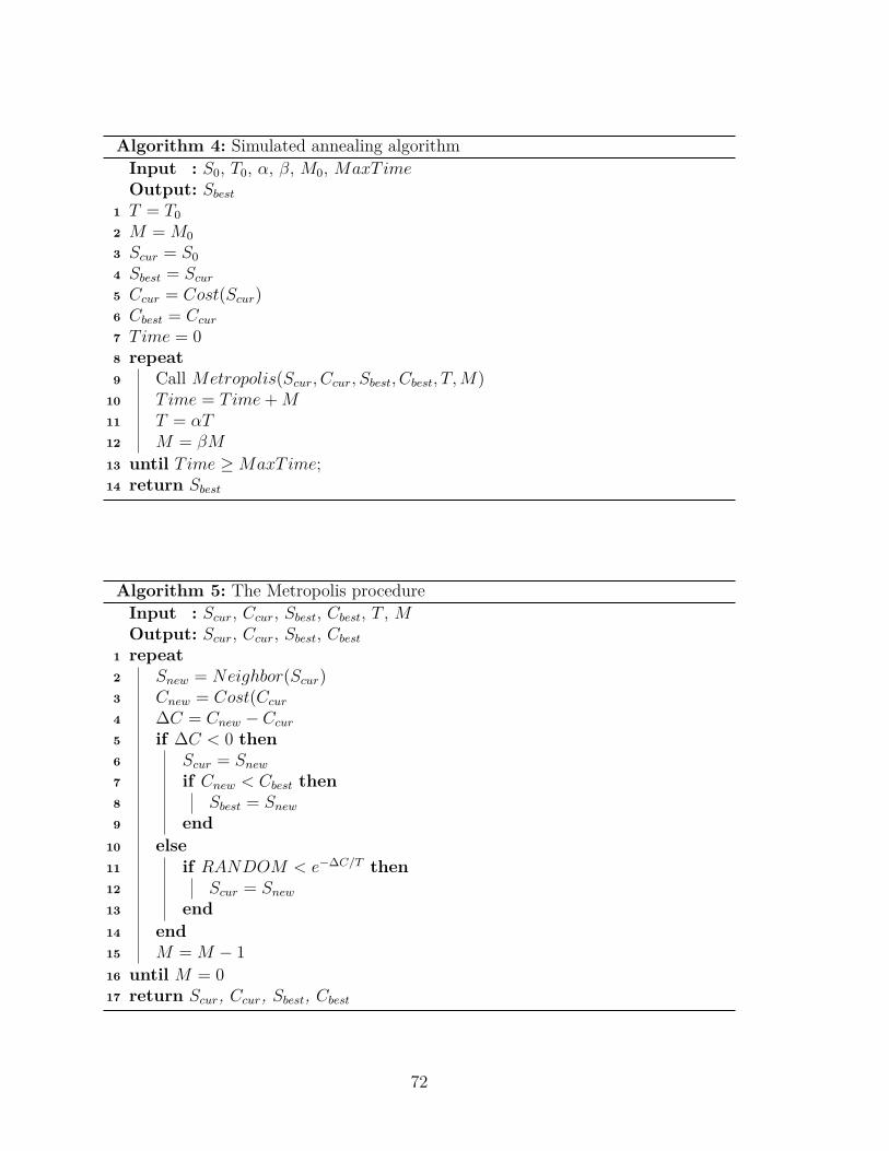
4.2 Simulated Annealing

Simulated annealing (SA) is a metaheuristic introduced by Kirpatrick et al. [70] in

1983, and independently by Černy [71] in 1985 to solve optimization problems with

large search spaces. The general structure of the SA and the Metropolis procedure are

shown in Algorithms 4 and 5 respectively [72]. The input to the algorithm consists

of 6 parameters (S0, T0, α, β, M0, MaxTime). The algorithm starts from an initial

solution S0 which can be generated randomly. In the beginning of the procedure, the

temperature is set to an initial value T0, and is decreased gradually using a cooling

65

rate α. The value of α is typically chosen in the range of 0.8 ≤ α ≤ 0.99. The initial

value of the time spent in the annealing process at a certain temperature is given

by the parameter M0. This time is gradually increased as the temperature decreases

using the parameter β. The total time for the annealing process is represented by the

parameter MaxTime.

The Metropolis procedure mimics the annealing operation at a certain temperature

T . This procedures receives 6 inputs which are the current solution and its cost (Scur,

Ccur), the best solution seen so far and its cost (Sbest, Cbest), the current temperature

T , and the parameter M which represents the amount of time need to be spent by the

annealing process at temperature T . The Metropolis procedure uses the procedure

Neighbor to generate a new solution Snew by doing a minor modification to the current

solution Scur. The cost of the new solution is evaluated by the function Cost. If the

cost of the new solution Snew is better than the cost of the current solution Scur, then

the current solution is updated by accepting the new solution. The same statement

applies to the best solution seen so far Sbest. The Metropolis procedure may accept a

solution with a higher cost with a probability p < e−∆C/T where ∆C is the difference

between the costs of the new and current solutions.

4.3 Implementation Details

In this section, we discuss the implementation details of the main functions of the

simulated annealing for both DASA and TGSA.

66

4.3.1 The Neighbor Function

In the SA algorithm, the neighbor function generates a new solution by making a minor

modification to the current solution. In the direct application of the SA algorithm to

the RA problem, we have implemented a simple neighbor function that exchanges the

assignment of two time-slots selected randomly as illustrated in Algorithm 6. Such

approach can not be used in the Tetris model as it may generate invalid solutions due

to overlapping pieces. Thus, before placing a piece p in a row r, the neighbor function

needs to make sure that p does not overlap with any piece already in r.

The neighbor function for the Tetris-Game model is described in Algorithm 7. This

function selects a random piece pout from a random row tout, and places it into another

random row tin. The function checks for overlapping between pout and existing pieces

in tin, and moves those pieces to tout. The function repeats the process of exchanging

overlapping pieces between tout and tin until there are no more overlaps. The row tout

is selected randomly from 1 to T , while tin is selected randomly from 1 to Ts, where

Ts is the total number of rows in the Tetris board (i.e., Tetris solution). In this way,

the TGSA algorithm can pack the pieces into T rows (time-slots) while maximizing

the total data rate.

4.3.2 The Cost Function

The cost function in SA computes the objective function to be minimized or maxi-

mized. In the RA problem, our objective is to maximize the total data rate under the

consideration of partial fairness as given in equation (2.9. The objective function can

67

be computed is shown in Algorithm 9. We have implemented two cost functions for

both DASA and TGSA:

1. Full Cost Function: evaluates the objective function for the whole solution based

on equation (2.9) as shown in Algorithms. This function needs to be applied

only once on the initial solution.

2. Partial Cost Function: evaluates the objective function by recomputing the

SINR values for the modified slots of the neighbor solution as shown in Algo-

rithms.

In the DASA, the cost of the new solution (Cnew) is computed based on the on the

cost of the old solution (Cold) using the following formula:

Cnew =

Cold +∑

u∈{ux,uy}t∈{tx,ty}

log2(1 + SINRnew[u, t])

−∑

u∈{ux,uy}t∈{tx,ty}

log2(1 + SINRold[u, t])

tx ≤ T

Cold +∑

u∈{ux,uy}t=ty

log2(1 + SINRnew[u, t])

−∑

u∈{ux,uy}t=ty

log2(1 + SINRold[u, t])

tx > T

(4.1)

where ux and uy are the two exchanged user assignments in time-slots tx and

ty respectively, and SINRnew and SINRold are the SINR values computed based on

the assignments in the new and old solutions respectively. Note that assignments in

time-slots greater than T do not affect the calculation of the cost function.

68

In the TGSA, the cos tis computed using the following formula:

Cnew =

Cold +∑

u∈{uin∪uout}t∈{tin,tout}

log2(1 + SINRnew[u, t])

−∑

u∈{uin∪uout}t∈{tin,tout}

log2(1 + SINRold[u, t])

tout ≤ T

Cold +∑

u∈{uin∪uout}t=tin

log2(1 + SINRnew[u, t])

−∑

u∈{uin∪uout}t=tin

log2(1 + SINRold[u, t])

tout > T

(4.2)

where uin and uout are the set of users assigned to time-slots tin and tout respectively.

69

Algorithm 2: Generates the initial solution in the direct implementationInput : M , N , T , KOutput: Sinit

1 /* Determine the number of slots available for each user */2 n← (K ×N × T )/M3 /* Generate an array from the set of users with each user repeated

n times */4 A← {1, 2, . . . ,M}n5 /* Arrange the elements of A in random order */6 A← RandomPermutation(A)7 /* Assign the elements of A to the slots in the solution */8 k ← 19 for i← 1 to N do

10 for j ← 1 to K × T do11 Sinit[i, j]← A[k]12 k ← k + 1

13 end14 end15 return Sinit

70

Algorithm 3: Generates the initial solution in the Tetris-Game modelInput : M , N , T , K, TetrisOutput: Sinit

1 n← length(Tetris)2 /* Generate an array from the set of piece's indices in Tetris

with each index repeated K times */3 A← {1, 2, . . . , n}K4 /* Arrange the elements of A in random order */5 A← RandomPermutation(A)6 /* Initialize the solution */7 for i← 1 to K × n do8 S[i].Assignment← (0, 0, . . . , 0)9 S[i].P ieces← ϕ

10 end11 /* Pack the pieces idexed by A into the rows of Sinit in a

first-fit manner */12 k ← 113 for i← 1 to K × n do14 index← A[k]15 piece← Tetris[index].P iece16 k ← k + 117 for j ← 1 to K × n do18 /* Check for overlapping between the piece and the

assignment in the jth row */19 overlap← S[j].Assignment ∧ piece20 if ¬overlap then21 /* Merge the piece with the current assignment */22 S[j].Assignment← S[j].Assignment ∨ piece23 /* Add the index of the piece to the list of pieces in

the jth row */24 S[j].P ieces← S[j].P ieces ∪ {index}25 break26 end27 end28 /* Copy none empty rows in S into Sinit */29 k ← 130 for i← 1 to K × n do31 if S[i].Assignment ̸= (0, 0, . . . , 0) then32 Sinit[k] = S[i]33 k ← k + 1

34 end35 return Sinit

71

Algorithm 4: Simulated annealing algorithmInput : S0, T0, α, β, M0, MaxTimeOutput: Sbest

1 T = T02 M =M0

3 Scur = S0

4 Sbest = Scur

5 Ccur = Cost(Scur)6 Cbest = Ccur

7 Time = 08 repeat9 Call Metropolis(Scur, Ccur, Sbest, Cbest, T,M)

10 Time = Time+M11 T = αT12 M = βM

13 until Time ≥MaxTime;14 return Sbest

Algorithm 5: The Metropolis procedureInput : Scur, Ccur, Sbest, Cbest, T , MOutput: Scur, Ccur, Sbest, Cbest

1 repeat2 Snew = Neighbor(Scur)3 Cnew = Cost(Ccur

4 ∆C = Cnew − Ccur

5 if ∆C < 0 then6 Scur = Snew

7 if Cnew < Cbest then8 Sbest = Snew

9 end10 else11 if RANDOM < e−∆C/T then12 Scur = Snew

13 end14 end15 M =M − 1

16 until M = 017 return Scur, Ccur, Sbest, Cbest

72

Algorithm 6: The neighbor function for DASA AlgorithmInput : S, N , T , KOutput: S

1 /* Select two different random slots from S */2 repeat3 tx ← RandomInteger(1..K × T )4 ty ← RandomInteger(1..T )5 dx ← RandomInteger(1..N)6 dy ← RandomInteger(1..N)

7 until tx ̸= ty or dx ̸= dy8 /* Exchange the two slots */9 Swap(S[dx, tx], S[dy, ty])

10 return S

73

Algorithm 7: The neighbor function for TGSA AlgorithmInput : S, N , T , TetrisOutput: S

1 /* Get the total length of the solution S */2 Ns ← |S|3 /* Select two different random rows from S */4 repeat5 tout ← RandomInteger(1..Ts)6 tin ← RandomInteger(1..T )

7 until tout ̸= tin8 /* Select a random piece from tout */9 pout ← S[tout].P ieces[RandomInteger(1..Ns)]

10 /* Initialize lists */11 check_list← {pout}12 move_list_pieces← ϕ13 move_list_rows← ϕ14 MoveList(check_list,move_list_pieces,move_list_rows, tin, tout, S, Tetris)15 /* Place pieces in move list in their proper rows */16 for each p ∈ move_list_pieces and t ∈ move_list_rows do17 /* Get the piece details from the Tetris */18 piece← Tetris[p].P iece19 /* Place the piece */20 S[t].Assignment = piece ∨ S[t].Assignment21 S[t].P ieces = S[t].P ieces ∪ p22 end23 /* Check if tout row is empty, then delete it */24 if S[tout].P ieces = ϕ then25 Delete(S[tout])26 end27 return S

74

Algorithm 8: The MoveList procedureInput : check_list, move_list_pieces, move_list_rows, tin, tout, S, TetrisOutput: move_list_pieces, move_list_rows

1 overlap_list← ϕ2 /* Determine overlaps between tin and tout due to moving pout */3 while check_list ̸= ϕ do4 /* Remove one element from the check list */5 pout ← check_list[1]6 checklist← check_list− pout7 /* Get the corresponding piece from Tetris */8 piece_out← Tetris[pout].P iece9 /* Remove the piece from tout */

10 S[tout].Assignment← S[tout].Assignment∧ ̸ piece11 /* Add pout to move lists in order to place it at tin */12 move_list_pieces← move_list_pieces ∪ pout13 move_list_rows← move_list_rows ∪ tin14 /* Find pieces at tin overlapping with pout */15 for Each pin ∈ S[tin].P ieces do16 /* Get the corresponding piece from Tetris */17 piece_in← Tetris[pin].P iece18 /* Check if piece_out and piece_in overlaps */19 if piece_out ∧ piece_in then20 /* Add pin to overlap_list */21 overlap_list← overlap_list ∪ pin22 end23 end24 /* Switch the process between tin and tout */25 check_list← overlap_list26 overlap_list← ϕ27 Swap(tin, tout)

28 end29 return move_list_pieces, move_list_rows

75

Algorithm 9: The full cost function for DASAInput : S, M , N , T , H, E, R, σOutput: C, M ′ , assigned_users

1 C ← 02 /* Compute the sum of channel-gains for each user */3 for u← 1 to M do4 h_sum[u]← Sum(H[u, 1..N ])5 end6 /* Initialize channel response and interference for all users */7 hr[1..M, 1..T ]← 08 hi[1..M, 1..T ]← h_sum[1..M ]9 /* Initialize the count of users assigned t time-slots 1 to T */

10 assigned_users[1..M ]← 011 /* Compute channel response and interference for each user */12 for d← 1 to N do13 for t← 1 to T do14 u← S[d, t]15 hr[u, t]← hr[u, t] +H[u, d]16 hi[u, t]← hi[u, t]−H[u, d]17 assigned_users[u]← assigned_users[u] + 1

18 end19 end20 for u← 1 to M do21 /* Compute the objective function */22 for t← 1 to T do23 SINR← ER2(hr[u, t])

2/(ER2(hi[u, t])2 + σ)

24 C ← C + log2(1 + SINR)

25 end26 /* Compute the number of users out of M assigned to time-slots

1 to T */27 if assigned_users[u] > 0 then28 M

′ ←M′+ 1

29 end30 end31 return C, M ′, assigned_users

76

Algorithm 10: The full cost function for TGSAInput : S, Tetris, M , N , T , H, E, R, σOutput: C, M ′ , assigned_users

1 C ← 02 /* Compute the sum of channel-gains for each user */3 for u← 1 to M do4 h_sum[u]← Sum(H[u, 1..N ])5 end6 /* Initialize channel response and interference for all users */7 hr[1..M, 1..T ]← 08 hi[1..M, 1..T ]← h_sum[1..M ]9 /* Initialize the count of users assigned t time-slots 1 to T */

10 assigned_users[1..M ]← 011 /* Compute channel response and interference for each user */12 for t← 1 to T do13 for each p ∈ S[t].P ieces do14 u← Tetris[p].User15 assigned_users[u]← assigned_users[u] + 116 piece← Tetris[p].P iece17 for each d ∈ piece do18 hr[u, t]← hr[u, t] +H[u, d]19 hi[u, t]← hi[u, t]−H[u, d]

20 end21 end22 end23 for u← 1 to M do24 /* Compute the objective function */25 for t← 1 to T do26 SINR← ER2(hr[u, t])

2/(ER2(hi[u, t])2 + σ)

27 C ← C + log2(1 + SINR)

28 end29 /* Compute the number of users out of M assigned to time-slots

1 to T */30 if assigned_users[u] > 0 then31 M

′ ←M′+ 1

32 end33 end34 return C, M ′, assigned_users

77

Algorithm 11: The partial cost function for DASAInput : Sold, Snew, Cold, M

′

old, assigned_users_old, N , T , tx, ty, ux, uy, H,E, R, σ

Output: Cnew, M ′new, assigned_users_new

1 Cnew ← Cold; M′new ←M

′

old

2 assigned_users_new ← assigned_users_old3 /* If ux and uy are identical, then the cost will be the same */4 if ux = uy then return Cnew, M ′

new, assigned_users_new5 /* Initialization */6 InitPartialCost(N , T , tx, ty, ux, uy, H)7 /* Update users counts */8 if tx > T then9 assigned_users_new[ux]← assigned_users_new[ux] + 1

10 assigned_users_new[uy]← assigned_users_new[uy]− 1

11 if assigned_users_new[ux] = 1 then M′new ←M

′new + 1

12 if assigned_users_new[uy] = 0 then M′new ←M

′new − 1

13 end14 /* Compute channel response and interference for each user */15 for d← 1 to N do16 for j ← 1 to |tc| do17 uold ← Sold[d, tc[j]] ; unew ← Snew[d, tc[j]]18 for i← 1 to |uc| do19 if uold = uc[i] then20 holdr [i, j]← holdr [i, j] +H[i, d]; holdi [i, j]← holdi [i, j]−H[i, d]21 end22 if unew = uc[i] then23 hnewr [i, j]← hnewr [i, j] +H[i, d]; hnewi [i, j]← hnewi [i, j]−H[i, d]24 end25 end26 end27 end28 /* Update the objective function */29 for i← 1 to |uc| do30 for j ← 1 to |tc| do31 SINRold ← ER2(holdr [i, j])2/(ER2(holdi [i, j])2 + σ)32 SINRnew ← ER2(hnewr [i, j])2/(ER2(hnewi [i, j])2 + σ)33 Cnew ← Cnew + log2(1 + SINRnew)− log2(1 + SINRold)

34 end35 end36 return Cnew, M ′

new, assigned_users_new

78

Algorithm 12: The procedure InitPartialCost for DASAInput : N , T , tx, ty, ux, uy, HOutput: tc, uc, holdr , holdi , hnewr , hnewi

1 /* Initialize users lists */2 uc ← {uy, ux}3 /* Initialize time-slots lists */4 if tx ≤ T then5 /* Both slots will affect the cost, but not the user's counts

*/6 tc ← {ty, tx}7 else8 /* Only ty will affect the cost */9 tc ← {ty}

10 end11 /* Compute the sum of channel-gains for the 2 user */12 for i← 1 to 2 do13 h_sum[i]← Sum(H[uc[i], 1..N ])14 end15 /* Initialize channel response and interference for the 2 users */16 holdr [1..2, 1..2]← 017 holdi [1..2, 1..2]← h_sum[1..2]18 hnewr [1..2, 1..2]← 019 hnewi [1..2, 1..2]← h_sum[1..2]20 return tc, uc, holdr , holdi , hnewr , hnewi

79

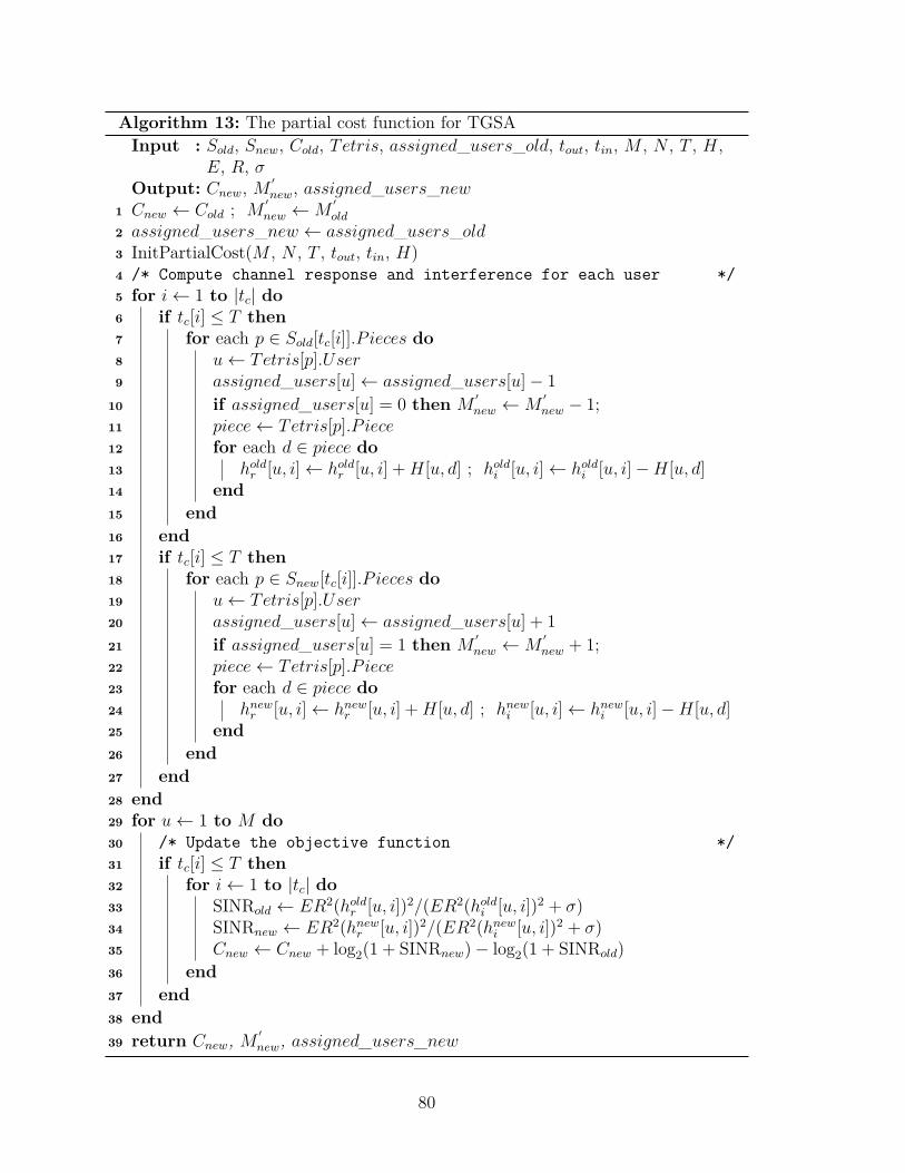
Algorithm 13: The partial cost function for TGSAInput : Sold, Snew, Cold, Tetris, assigned_users_old, tout, tin, M , N , T , H,

E, R, σOutput: Cnew, M ′

new, assigned_users_new1 Cnew ← Cold ; M

′new ←M

′

old

2 assigned_users_new ← assigned_users_old3 InitPartialCost(M , N , T , tout, tin, H)4 /* Compute channel response and interference for each user */5 for i← 1 to |tc| do6 if tc[i] ≤ T then7 for each p ∈ Sold[tc[i]].P ieces do8 u← Tetris[p].User9 assigned_users[u]← assigned_users[u]− 1

10 if assigned_users[u] = 0 then M′new ←M

′new − 1;

11 piece← Tetris[p].P iece12 for each d ∈ piece do13 holdr [u, i]← holdr [u, i] +H[u, d] ; holdi [u, i]← holdi [u, i]−H[u, d]14 end15 end16 end17 if tc[i] ≤ T then18 for each p ∈ Snew[tc[i]].P ieces do19 u← Tetris[p].User20 assigned_users[u]← assigned_users[u] + 1

21 if assigned_users[u] = 1 then M′new ←M

′new + 1;

22 piece← Tetris[p].P iece23 for each d ∈ piece do24 hnewr [u, i]← hnewr [u, i] +H[u, d] ; hnewi [u, i]← hnewi [u, i]−H[u, d]25 end26 end27 end28 end29 for u← 1 to M do30 /* Update the objective function */31 if tc[i] ≤ T then32 for i← 1 to |tc| do33 SINRold ← ER2(holdr [u, i])2/(ER2(holdi [u, i])2 + σ)34 SINRnew ← ER2(hnewr [u, i])2/(ER2(hnewi [u, i])2 + σ)35 Cnew ← Cnew + log2(1 + SINRnew)− log2(1 + SINRold)

36 end37 end38 end39 return Cnew, M ′

new, assigned_users_new

80

Algorithm 14: The procedure InitPartialCost for TGSAInput : M , N , T , tout, tin, HOutput: tc, holdr , holdi , hnewr , hnewi

1 /* Initialize time-slots lists */2 if tout ≤ T then3 /* Both slots will affect the cost, but not the users counts */4 tc ← {tin, tout}5 else6 /* Only tin will affect the cost */7 tc ← {tin}8 end9 /* Compute the sum of channel-gains for all users */

10 for u← 1 to M do11 h_sum[u]← Sum(H[u, 1..N ])12 end13 /* Initialize channel response and interference for all users */14 holdr [1..M, 1..2]← 015 holdi [1..M, 1..2]← h_sum[1..M ]16 hnewr [1..M, 1..2]← 017 hnewi [1..M, 1..2]← h_sum[1..M ]18 return tc, holdr , holdi , hnewr , hnewi

81

CHAPTER 5

NUMERICAL RESULTS AND

DISCUSSION

As discussed in Chapter 4, we have developed two metaheuristics for the indoor re-

source allocation problem. The first algorithm is a direct application of the simulated

annealing (DASA) and the second is a simulated annealing algorithm based on the

Tetris-Game model (TGSA). In this chapter, we present the experimental results based

on these algorithms.

5.1 Indoor RA Optimization

In our simulation of the proposed model for indoor environment, we have considered

a room of size 12.0m× 12.0m× 3.0m with 16 LEDs on the ceiling spaced by 3.0m in

both directions as illustrated in Fig. 5.1. The number of users is varied from 16 to 64

and are randomly distributed in the room. Table 5.1 shows the system and channel

parameters used in our experiments [67]. The transmission power for each LED (P ) is

82

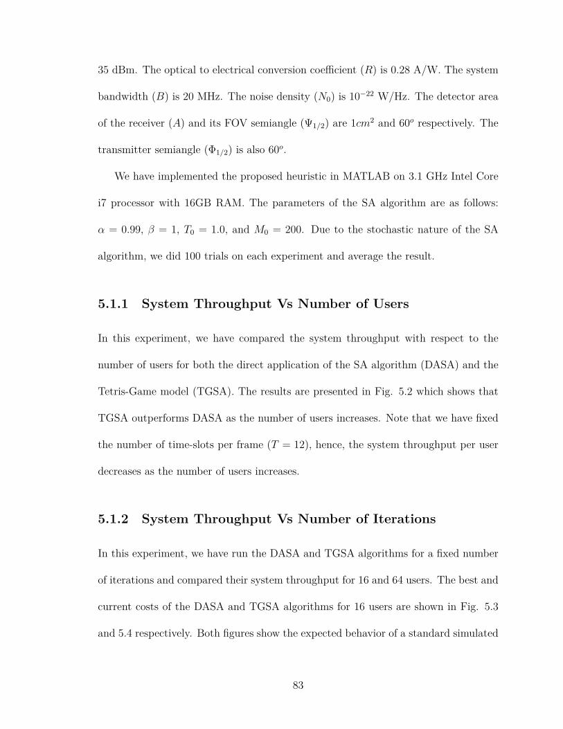
35 dBm. The optical to electrical conversion coefficient (R) is 0.28 A/W. The system

bandwidth (B) is 20 MHz. The noise density (N0) is 10−22 W/Hz. The detector area

of the receiver (A) and its FOV semiangle (Ψ1/2) are 1cm2 and 60o respectively. The

transmitter semiangle (Φ1/2) is also 60o.

We have implemented the proposed heuristic in MATLAB on 3.1 GHz Intel Core

i7 processor with 16GB RAM. The parameters of the SA algorithm are as follows:

α = 0.99, β = 1, T0 = 1.0, and M0 = 200. Due to the stochastic nature of the SA

algorithm, we did 100 trials on each experiment and average the result.

5.1.1 System Throughput Vs Number of Users

In this experiment, we have compared the system throughput with respect to the

number of users for both the direct application of the SA algorithm (DASA) and the

Tetris-Game model (TGSA). The results are presented in Fig. 5.2 which shows that

TGSA outperforms DASA as the number of users increases. Note that we have fixed

the number of time-slots per frame (T = 12), hence, the system throughput per user

decreases as the number of users increases.

5.1.2 System Throughput Vs Number of Iterations

In this experiment, we have run the DASA and TGSA algorithms for a fixed number

of iterations and compared their system throughput for 16 and 64 users. The best and

current costs of the DASA and TGSA algorithms for 16 users are shown in Fig. 5.3

and 5.4 respectively. Both figures show the expected behavior of a standard simulated

83

0 3 6 9 12

0

3

6

9

12

Figure 5.1: Distribution of LEDs in the room.

84

Table 5.1: System and channel parameters.Parameter Symbol ValueTransmission Power for each LED P 20 dBmO/E Conversion Coefficient R 0.28 A/WSystem Bandwidth B 5 MHzNoise Density N0 10−22 W/HzDetector Area (A) 1cm2

Receiver FOV Semiangle Ψ1/2 60o

Transmitter Semiangle Φ1/2 60o

85

16 24 32 48 64

Number of Users

0

20

40

60

80

100

120

140

160

180

Syst

em D

ata

Rat

e [M

bps]

DASA

TGSA

Figure 5.2: System throughput with respect to the number of users.

86

annealing algorithm with hill-climbing. Fig. 5.5 and 5.6 show comparisons between

the best cost of the TGSA and that of DASA for 16 and 64 users respectively. These

results show that the Tetris-Game model improves both the solution quality and the

convergence rate.

5.2 Underwater RA Optimization

We consider the same setup as for the indoor environment except that users can move

in the vertical direction. Assuming a pure water and LOS, the channel response can

be calculated as given in equation (2.6). Fig. 5.7 shows a comparison between the best

cost of TGSA and DASA for 16 users in underwater environment. The results show

a similar behaviour of both algorithms where TGSA converges faster than DASA.

5.3 Results Discussion and Future Work

Our experiments using standard simulated annealing algorithm show that the final

allocation of LEDs takes a form similar to the arrangement of the Tetris pieces. This

is illustrated in in Table 5.2 for an indoor environment with nine LEDs (N = 9), eight

users (M = 8) and eight time-slots per frame (T = 8). The channel-gains of the users

are shown in Table 5.3. This observation is consistent with the results obtained in

Section 5.1.2 which show clearly that TGSA converges faster than DASA as it operates

on groups of assignments rather than individual ones.

In future work, we are planning to investigate more meta-heuristics and optimize

the proposed algorithms to satisfy the the channel coherence time. In addition to that,

87

0 200 400 600 800 1000 1200 1400

Number of Iterations

50

100

150

200

250

300

350

400

450

500

550

Syst

em D

ata

Rat

es

DASA Current Cost

DASA Best Cost

Figure 5.3: Best and current costs of the DASA for 16 users.

88

0 200 400 600 800 1000 1200 1400

Number of Iterations

380

400

420

440

460

480

500

520

540

560

Syst

em D

ata

Rat

e

TGSA Best Cost

TGSA Current Cost

Figure 5.4: Best and current costs of the TGSA for 16 users.

89

0 200 400 600 800 1000 1200 1400

Number of Iterations

50

100

150

200

250

300

350

400

450

500

550

Syst

em D

ata

Rat

e

DASA Best Cost

TGSA Best Cost

Figure 5.5: Comparison of the best costs of TGSA and DASA for 16 users.

90

0 200 400 600 800 1000 1200 1400

Number of Iterations

0

100

200

300

400

500

Syst

em D

ata

Rat

e

TGSA Best Cost

DASA Best Cost

Figure 5.6: Comparison of the best costs of TGSA and DASA for 64 users.

91

0 200 400 600 800 1000 1200 1400

Number of Iterations

0

100

200

300

400

500

600

Syst

em D

ata

Rat

e

TGSA Best Cost

DASA Best Cost

Figure 5.7: Comparison of the best costs of TGSA and DASA for 16 users in under-water environment.

92

we will develop optimization heuristics for different types of water for the underwater

VLC problem (In our experiments, we considered only pure water types).

93

Table 5.2: Allocation result from a standard simulated annealing implementation for8 users, 9 LEDs and 8 time-slots per frame (M = 8, N = 9, T = 8).

T1 T2 T3 T4 T5 T6 T7 T8D1 6 6 6 6 6 6 6 6D2 6 6 6 6 6 6 6 6D3 4 4 4 4 4 4 4 4D4 1 5 1 1 1 1 1 3D5 1 8 1 1 1 1 1 8D6 4 4 4 4 4 4 4 4D7 1 8 1 1 1 1 1 8D8 1 8 1 1 1 1 1 8D9 7 8 7 7 7 2 7 8

Table 5.3: Channel-gains of the example shown in Table 5.2.D1 D2 D3 D4 D5 D6 D7 D8 D9

U1 0 0 0 0.1012 0.1218 0 0.2165 0.2856 0U2 0 0 0 0 0.0861 0.2135 0 0.1113 0.3247U3 0.0517 0.5205 0.1312 0 0.1004 0.0487 0 0 0U4 0 0 0.1268 0 0 0.2453 0 0 0U5 0 0 0 0 0.18 0.0791 0.0426 0.3649 0.1227U6 0.2732 0.214 0 0 0 0 0 0 0U7 0 0 0 0 0.0414 0.05 0 0.2226 0.3539U8 0 0 0 0 0.064 0.0392 0.0447 0.4836 0.1557

94

APPENDIX A

SUPPLEMENTARY MATERIAL

A.1 MATLAB Code: Direct Application Simu-

lated Annealing

%% Parametersglobal L W H LED PD M N T S A h h_sum E R sigma BW X;

% TDMA parametersM = 8 ; % number o f u s e r sN = 9 ; % number o f LEDsT = 8 ; % number o f time−s l o t sS = N ∗ T; % t o t a l number o f s l o t sA = f loor (S/M) ; % number o f s l o t s per userX = 16 ;L = 9 ; % room l e n g t hW = 9 ; % room widthH = 3 ; % room h e i g h t

E_dBm = 20 ; % symbol energy in dBmE = db2pow (E_dBm−30); % symbol energy in Watt 10 log_10 ( y )R = 0 . 2 8 ; % o p t i c a l to e l e c t r i c a l conver s i on

% c o e f f i c i e n tBW = 5e +6; % system bandwidth in Hz ( per LED)sigma = (1 e−22) ∗ BW; % no i s e power in Watt

95

squa r e s = sqrt (N) ; % number o f s quare s in each% row/column in the room

s t ep = L/ squa r e s ; % s e p a r a t i o n d i s t a n c e between% two LEDs

s t a r t = s t ep /2 ; % s t a r t i n g l o c a t i o n o f t he 1 s t LEDx = s t a r t : s t ep : L ; % x c o o r d i n a t e s o f t he LEDsy = x ; % y c o o r d i n a t e s o f t he LEDs

% compute the x−y−z c o o r i n a t e s o f t he LEDsLED = zeros (N, 3 ) ;LED( : , 3 ) = H;LED( : , 1 : 2 ) = combvec (x , y ) ’ ;

% genera t e x−y−z c o o r d i n a t e s o f t he u s e r s ( photo−d i ode s )PD = [ round ( rand (M, 1 ) ∗ L , 2 ) , . . .

round ( rand (M, 1 ) ∗W, 2 ) , . . .round ( 0 . 7 ∗ ones (M, 1 ) , 2 ) ] ;

% g e t channe l r e sponse sh = compute_channel_responses ( ) ;

load ( ’ v l c 8 . mat ’ , ’PD ’ , ’ h ’ ) ;

h_sum = sum(h , 2 ) ;

%% Simula ted Anneal ing Funct ions o l u t i o n = generate_random_solut ion ( ) ;% SA ParametersS0 = s o l u t i o n ; % i n i t i a l s o l u t i o nT0 = 1 ; % i n i t i a l t empera tureTf = 1 . 0 e−3; % f i n a l t empera turealpha = 0 . 9 9 5 ; % c o o l i n g r a t ebeta = 1 ; % cons tan tTp = 200 ; % time u n t i l t h e nex t

% parameter% update

Tc = T0 ; % curren t tempera tureCurS = S0 ; % curren t s o l u t i o nBestS = S0 ; % b e s t s o l u t i o n seenCurC = CurS . c o s t ∗ CurS . count / M; % curren t c o s tBestC = CurC ; % b e s t c o s t seenMaxIter = c o u n t _ i t e r a t i o n s (T0 , Tf , a lpha ) ;DASA_CC = zeros ( 1 , MaxIter ) ;DASA_BB = zeros ( 1 , MaxIter ) ;I t e r = 1 ;

96

while Tc > Tfcount = 0 ;while count < Tp

NewS = ne ighbor ( CurS ) ;NewC = NewS . c o s t ∗ NewS . count / M;DeltaC = NewC − CurC ;i f DeltaC > 0

CurS = NewS ;CurC = NewC;i f NewC > BestC

BestS = NewS ;BestC = NewC;

ende l s e i f rand <= exp ( DeltaC/Tc)

CurS = NewS ;CurC = NewC;

endcount = count + 1 ;

endDASA_CC_16( I t e r ) = CurC ;DASA_BB_16( I t e r ) = BestS . c o s t ;I t e r = I t e r + 1 ;

Tc = alpha ∗ Tc ;Tp = beta ∗ Tp ;

endfigure ( 1 ) ;p l o t _ s o l u t i o n ( BestS , 0 . 0 , BestC , 0 . 0 ) ;f igure ( 2 ) ;plot (DASA_CC) ;f igure ( 3 ) ;plot (DASA_BB) ;

%% Count Number o f I t e r a t i o n sfunction n = c o u n t _ i t e r a t i o n s (T0 , Tf , a lpha )n = 0 ;Tc = T0 ;while Tc > Tf

Tc = Tc ∗ alpha ;n = n + 1 ;

endend

%% Compute Cost ( F i t n e s s )

97

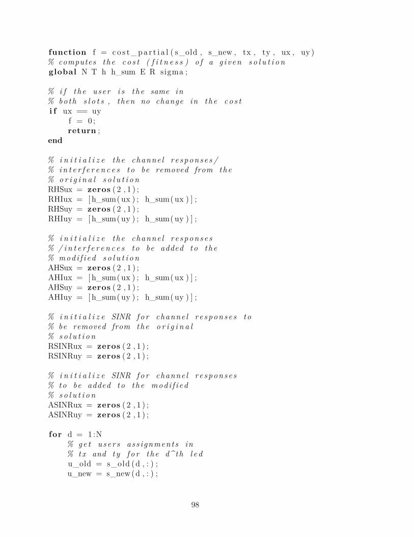
function f = c o s t _ p a r t i a l ( s_old , s_new , tx , ty , ux , uy )% computes the c o s t ( f i t n e s s ) o f a g i v en s o l u t i o nglobal N T h h_sum E R sigma ;

% i f the user i s t he same in% both s l o t s , then no change in the c o s ti f ux == uy

f = 0 ;return ;

end

% i n i t i a l i z e t he channe l r e sponse s /% i n t e r f e r e n c e s to be removed from the% o r i g i n a l s o l u t i o nRHSux = zeros ( 2 , 1 ) ;RHIux = [ h_sum( ux ) ; h_sum( ux ) ] ;RHSuy = zeros ( 2 , 1 ) ;RHIuy = [ h_sum( uy ) ; h_sum( uy ) ] ;

% i n i t i a l i z e t he channe l r e sponse s% / i n t e r f e r e n c e s to be added to the% mod i f i ed s o l u t i o nAHSux = zeros ( 2 , 1 ) ;AHIux = [ h_sum( ux ) ; h_sum( ux ) ] ;AHSuy = zeros ( 2 , 1 ) ;AHIuy = [ h_sum( uy ) ; h_sum( uy ) ] ;

% i n i t i a l i z e SINR f o r channe l r e sponse s to% be removed from the o r i g i n a l% s o l u t i o nRSINRux = zeros ( 2 , 1 ) ;RSINRuy = zeros ( 2 , 1 ) ;

% i n i t i a l i z e SINR f o r channe l r e sponse s% to be added to the mod i f i ed% s o l u t i o nASINRux = zeros ( 2 , 1 ) ;ASINRuy = zeros ( 2 , 1 ) ;

for d = 1 :N% g e t u s e r s ass i gnments in% t x and ty f o r the d^ th l e du_old = s_old (d , : ) ;u_new = s_new (d , : ) ;

98

% r e c a l c u l a t i o n f o r t ime s l o t t x w i l l% be done i f and on ly i f t x <= T and t x ~= tyi f tx <= T && tx ~= ty

i f u_old (1 ) == uxRHSux(1 ) = RHSux(1 ) + h( ux , d ) ;RHIux (1 ) = RHIux (1 ) − h( ux , d ) ;

e l s e i f u_old (1 ) == uyRHSuy(1 ) = RHSuy(1 ) + h( uy , d ) ;RHIuy (1 ) = RHIuy (1 ) − h( uy , d ) ;

end

i f u_new (1 ) == uxAHSux(1 ) = AHSux(1 ) + h( ux , d ) ;AHIux (1 ) = AHIux (1 ) − h( ux , d ) ;

e l s e i f u_new (1 ) == uyAHSuy(1 ) = AHSuy(1 ) + h( uy , d ) ;AHIuy (1 ) = AHIuy (1 ) − h( uy , d ) ;

endend

% r e c a l c u l a t i o n f o r t ime s l o t% ty w i l l be done in a l l c a s e si f u_old (2 ) == ux

RHSux(2 ) = RHSux(2 ) + h( ux , d ) ;RHIux (2 ) = RHIux (2 ) − h( ux , d ) ;

e l s e i f u_old (2 ) == uyRHSuy(2 ) = RHSuy(2 ) + h( uy , d ) ;RHIuy (2 ) = RHIuy (2 ) − h( uy , d ) ;

end

i f u_new (2 ) == uxAHSux(2 ) = AHSux(2 ) + h( ux , d ) ;AHIux (2 ) = AHIux (2 ) − h( ux , d ) ;

e l s e i f u_new (2 ) == uyAHSuy(2 ) = AHSuy(2 ) + h( uy , d ) ;AHIuy (2 ) = AHIuy (2 ) − h( uy , d ) ;

end

end

% compute SINR f o r% removed channe l r e sponse sRSINRux (1 ) = E ∗ R^2 ∗ RHSux(1)^2 / . . .(E ∗ R^2 ∗ RHIux (1)^2 + sigma ) ;RSINRux (2 ) = E ∗ R^2 ∗ RHSux(2)^2 / . . .

99

(E ∗ R^2 ∗ RHIux (2)^2 + sigma ) ;RSINRuy (1 ) = E ∗ R^2 ∗ RHSuy(1)^2 / . . .(E ∗ R^2 ∗ RHIuy (1)^2 + sigma ) ;RSINRuy (2 ) = E ∗ R^2 ∗ RHSuy(2)^2 / . . .(E ∗ R^2 ∗ RHIuy (2)^2 + sigma ) ;

% compute SINR f o r added channe l r e sponse sASINRux (1 ) = E ∗ R^2 ∗ AHSux(1)^2 / . . .(E ∗ R^2 ∗ AHIux (1)^2 + sigma ) ;ASINRux (2 ) = E ∗ R^2 ∗ AHSux(2)^2 / . . .(E ∗ R^2 ∗ AHIux (2)^2 + sigma ) ;ASINRuy (1 ) = E ∗ R^2 ∗ AHSuy(1)^2 / . . .(E ∗ R^2 ∗ AHIuy (1)^2 + sigma ) ;ASINRuy (2 ) = E ∗ R^2 ∗ AHSuy(2)^2 / . . .(E ∗ R^2 ∗ AHIuy (2)^2 + sigma ) ;

% compute c o s t inc rementa l v a l u ef = log2 (1 + ASINRux ( 1 ) ) + . . .

log2 (1 + ASINRux ( 2 ) ) + . . .log2 (1 + ASINRuy ( 1 ) ) + . . .log2 (1 + ASINRuy ( 2 ) ) − . . .log2 (1 + RSINRux ( 1 ) ) − . . .log2 (1 + RSINRux ( 2 ) ) − . . .log2 (1 + RSINRuy ( 1 ) ) − . . .log2 (1 + RSINRuy ( 2 ) ) ;

end

%% Compute Cost ( F i t n e s s )function f = c o s t _ f u l l ( s o l u t i o n )% computes the c o s t ( f i t n e s s ) o f a g i v en s o l u t i o nglobal M N T h h_sum E R sigma ;

% i n i t i a l i z e SINRSINR = zeros (M,T) ;

ov e r a l l_a s s i gn ed_us e r s = zeros (M, 1 ) ;for t = 1 :T

% i n i t i a l i z e channe l r e sponse s and% i n t e r f e r e n c e in the t ^ th time−s l o ths = zeros (M, 1 ) ;h i = h_sum ;

% i n i t i a l i z e s e t o f a s s i gn ed us e r scur r ent_as s i gned_use r s = f a l s e (M, 1 ) ;

100

for d = 1 :N% g e t user ass ignmentu = s o l u t i o n . ass ignment (d , t ) ;

% s k i p unass i gned s l o t si f u == 0

h i ( : ) = h i ( : ) − h ( : , d ) ;cont inue ;

end

% compute channe l r e sponse s and% i n t e r f e r e n c e f o r the u^ th userhs (u ) = hs (u ) + h(u , d ) ;h i ( u ) = h i (u ) − h(u , d ) ;

% add user to the a s s i gned us e r s s e tcur r ent_as s i gned_use r s (u ) = t rue ;ov e r a l l_a s s i gn ed_us e r s (u ) = 1 ;

end% compute SINR f o r u s e r s a s s i gned% in the t ^ th t ime s l o t sfor u = 1 :M

i f cur r ent_as s i gned_use r s (u )SINR(u , t ) = E ∗ R^2 ∗ hs (u)^2 / . . .(E ∗ R^2 ∗ h i (u)^2 + sigma ) ;

endend

end% compute data r a t e per userDR = sum( log2 (1+SINR ) , 2 ) ;% compute the t o t a l data r a t ef = sum(DR, ’ a l l ’ ) ;end

%% Create Neighborfunction s = ne ighbor ( s o l u t i o n )% c r e a t e s a new s o l u t i o n by exchang ing two ass i gnments s e l e c t e d randomlyglobal S X;s = s o l u t i o n ;

% s e l e c t two d i f f e r e n t s l o t s randomlys i = 0 ;s j = 0 ;

101

while s i == s js i = rand i (X∗S ) ;s j = rand i (S ) ;

end

s s = s ize ( s . ass ignment ) ;[ di , t i ] = ind2sub ( ss , s i ) ;[ dj , t j ] = ind2sub ( ss , s j ) ;

u i = s . ass ignment ( s i ) ;u j = s . ass ignment ( s j ) ;

% g e t ass i gnments in t i and t j b e f o r e exchanges_old = [ s . ass ignment ( : , t i ) s . ass ignment ( : , t j ) ] ;

% i f s i i s not in the f i r s t T time s l o t s ,% then update a s s i gned us e r s counti f s i > S

% i f u i i s not a s s i gn ed any s l o t% in the f i r s t T time s l o t s , then% increment u s e r s counti f s . u s e r s ( u i ) == 0

s . count = s . count + 1 ;end

% update u s e r s ass i gnments counts . u s e r s ( u i ) = s . u s e r s ( u i ) + 1 ;s . u s e r s ( u j ) = s . u s e r s ( u j ) − 1 ;

% i f u j i s not a s s i gn ed to any% s l o t in the f i r s t T time s l o t s , then% decrement u s e r s counti f s . u s e r s ( u j ) == 0

s . count = s . count − 1 ;end

end

% in t e r change t h e s e two s l o t stemp = s . ass ignment ( s i ) ;s . ass ignment ( s i ) = s . ass ignment ( s j ) ;s . ass ignment ( s j ) = temp ;

s_new = [ s . ass ignment ( : , t i ) s . ass ignment ( : , t j ) ] ;s . c o s t = s . c o s t + c o s t _ p a r t i a l ( s_old , s_new , . . .

102

t i , t j , ui , u j ) ;end

%% Generate Random S o l u t i o n% g e n e r a t e s a random s o l u t i o n wi th e qua l t ime s l o t s f o r each userfunction s = generate_random_solut ion ( )global M N T A S X;

% i n t i a l i z e s o l u t i o n s t r u c t u r e% ass ignment : matr ix o f i n t% user ass ignment matr ix (LEDs x Time S l o t s )% c o s t : f l o a t% c o s t o f t he s o l u t i o n% use r s : v e c t o r o f i n t% number o f ass i gnments to each user in the f i r s t T s l o t s% count : i n t% number o f u s e r s out o f M as s i gned to the f i r s t T s l o t ss = s t r u c t ( ’ ass ignment ’ , zeros (N,X∗T) , . . .

’ c o s t ’ , 0 . 0 , . . .’ u s e r s ’ , zeros (M, 1 ) , . . .’ count ’ , 0 ) ;

% genera t e A random samples o f u s e r susers_samples = zeros (X∗A,M) ;for i = 1 :X∗A

users_samples ( i , : ) = randsample (M,M) ’ ;end

% a s s i g n t h e s e random samples to the NxT s l o t sfor i = 1 :X∗S

% g e t a random useruse r = users_samples ( i ) ;

% increment a s s i gned us e r s count in a l l s l o t s <= Ti f i <= S

i f s . u s e r s ( u s e r ) == 0s . count = s . count + 1 ;

ends . u s e r s ( u s e r ) = s . u s e r s ( u s e r ) + 1 ;

end

% a s s i g n users . ass ignment ( i ) = use r ;

103

ends . c o s t = c o s t _ f u l l ( s ) ;end

%% Plo t Room% p l o t t he room wi th LEDs and PDsfunction f = plot_room ( )global M PD LED L W;shgf = 0 ;% p l o t LEDs ’ l o c a t i o n ss c a t t e r (LED( : , 1 ) , LED( : , 2 ) , ’ b ’ ) ;

% p l o t PDs ’ l o c a t i o n shold on ;s c a t t e r (PD( : , 1 ) , PD( : , 2 ) , ’ r ’ ) ;grid minor ;axis ( [ 0 L 0 W] )

% d i s p l y users ’ l a b e l su s e r s = ( 1 :M) ’ ;l a b e l s = num2str ( use r s , ’%d ’ ) ;text (PD( : , 1 ) , PD( : , 2 ) , l a b e l s , . . .’ h o r i z o n t a l ’ , ’ l e f t ’ , ’ v e r t i c a l ’ , ’ bottom ’ ) ;

drawnow ;end

%% Plo t S o l u t i o n% p l o t s o l u t i o n as a heat−mapfunction f = p l o t _ s o l u t i o n ( s o l u t i o n , CurC , BestC , t )global T;shgf = 0 ;heatmap ( s o l u t i o n . ass ignment ( : , 1 :T ) ) ;s t r = sprintf ( ’ Current : ␣%f , ␣ Best : ␣%f , ␣ . . .Temp : ␣%f ’ ,CurC , BestC , t ) ;%t i t l e ( s t r ) ;drawnow ;end

A.2 MATLAB Code: Tetris Game Model Simu-lated Annealing

104

%% Parametersglobal L W H LED PD M N T S A h E R sigma t e t r i s BW h_sum ;

% TDMA parametersM = 16 ; % number o f u s e r sN = 16 ; % number o f LEDsT = 12 ; % number o f time−s l o t sS = N ∗ T; % t o t a l number o f s l o t s%A = f l o o r (S/M) ; % number o f s l o t s per userA = 18 ; % number o f p i e c e s o f each t e t r i s

% combinat ionL = 12 ; % room l e n g t hW = 12 ; % room widthH = 3 ; % room h e i g h tE_dBm = 20 ; % symbol energy in dBmE = db2pow (E_dBm−30); % symbol energy in Watt10log_10 ( y )R = 0 . 2 8 ; % o p t i c a l to e l e c t r i c a l

% conver s i on c o e f f i c i e n tBW = 5e +6; % system bandwidth in Hz ( per LED)sigma = (1 e−22) ∗ BW; % no i s e power in Wattsqua r e s = sqrt (N) ; % number o f s quare s in each

% row/column in the rooms t ep = L/ squa r e s ; % s e p a r a t i o n d i s t a n c e

% between two LEDss t a r t = s t ep /2 ; % s t a r t i n g l o c a t i o n o f t he 1 s t LEDx = s t a r t : s t ep : L ; % x c o o r d i n a t e s o f t he LEDsy = x ; % y c o o r d i n a t e s o f t he LEDs

% compute the x−y−z c o o r i n a t e s o f t he LEDsLED = zeros (N, 3 ) ;LED( : , 3 ) = H;LED( : , 1 : 2 ) = combvec (x , y ) ’ ;

% genera t e x−y−z c o o r d i n a t e s o f t he u s e r s ( photo−d i ode s )PD = [ round ( rand (M, 1 ) ∗ L , 2 ) , . . .

round ( rand (M, 1 ) ∗W, 2 ) , . . .round ( 0 . 7 ∗ ones (M, 1 ) , 2 ) ] ;

% g e t channe l r e sponse sh = compute_channel_responses ( ) ;

load ( ’ v l c 16 . mat ’ , ’PD ’ , ’ h ’ ) ;

h_sum = sum(h , 2 ) ;

105

% compute t e t r i s p i e c e st e t r i s = compute_tet r i s_p iece s ( ) ;

%% Simula ted Anneal ing% gene ra t e an i n i t a l random s o l u t i o ns o l u t i o n = generate_random_solut ion ( ) ;

% SA ParametersS0 = s o l u t i o n ; % i n i t i a l s o l u t i o nT0 = 1 ; % i n i t i a l t empera tureTf = 1 . 0 e−3; % f i n a l t empera turealpha = 0 . 9 9 5 ; % c o o l i n g r a t ebeta = 1 ; % cons tan tTp = 200 ; % time u n t i l t h e nex t parameter update

Tc = T0 ; % curren t tempera tureCurS = S0 ; % curren t s o l u t i o nBestS = S0 ; % b e s t s o l u t i o n seen so f a rCurC = CurS . c o s t ∗ CurS . users_count / M; % curren t c o s tBestC = CurC ; % b e s t c o s t seen so f a r

MaxIter = c o u n t _ i t e r a t i o n s (T0 , Tf , a lpha ) ;TGSA_CC = zeros ( 1 , MaxIter ) ;TGSA_BB = zeros ( 1 , MaxIter ) ;I t e r = 1 ;

while Tc > Tfcount = 0 ;while count < Tp

NewS = ne ighbor ( CurS ) ;NewC = NewS . c o s t ∗ NewS . users_count / M;DeltaC = (NewC − CurC ) ;i f DeltaC > 0

CurS = NewS ;CurC = NewC;i f NewC > BestC

BestS = NewS ;BestC = NewC;

ende l s e i f rand <= exp ( DeltaC/Tc)

CurS = NewS ;CurC = NewC;

endcount = count + 1 ;

end

106

%p l o t _ s o l u t i o n (CurS , CurS . cos t , BestS . cos t , Tc ) ;

TGSA_CC( I t e r ) = CurC ;TGSA_BB( I t e r ) = BestC ;I t e r = I t e r + 1 ;Tc = alpha ∗ Tc ;Tp = beta ∗ Tp ;

endfigure ( 1 ) ;p l o t _ s o l u t i o n ( BestS , 0 . 0 , BestC , 0 . 0 ) ;f igure ( 2 ) ;plot (TGSA_CC) ;f igure ( 3 ) ;plot (TGSA_BB) ;

%% Count Number o f I t e r a t i o n sfunction n = c o u n t _ i t e r a t i o n s (T0 , Tf , a lpha )n = 0 ;Tc = T0 ;while Tc > Tf

Tc = Tc ∗ alpha ;n = n + 1 ;

endend%% Neighborfunction s = ne ighbor ( s o l u t i o n )% c r e a t e s a new s o l u t i o n by removing% one p i e c e randomly from the g i v en% s o l u t i o n and a s s i g n i n g i t aga in in a random orderglobal t e t r i s N T;s = s o l u t i o n ;n = length ( s . s l o t s ) ;%% s t e p ( 1 ) : s e l e c t two random time% s l o t s t_out and t_in and random p i e c e%% s e l e c t two random time s l o t st_out = 0 ;t_in = 0 ;while t_out == t_in

t_out = rand i (n ) ;t_in = rand i (T) ;

end% s e l e c t random p i e c eindex = rand i ( s . s l o t s ( t_out ) . p i eces_count ) ;

107

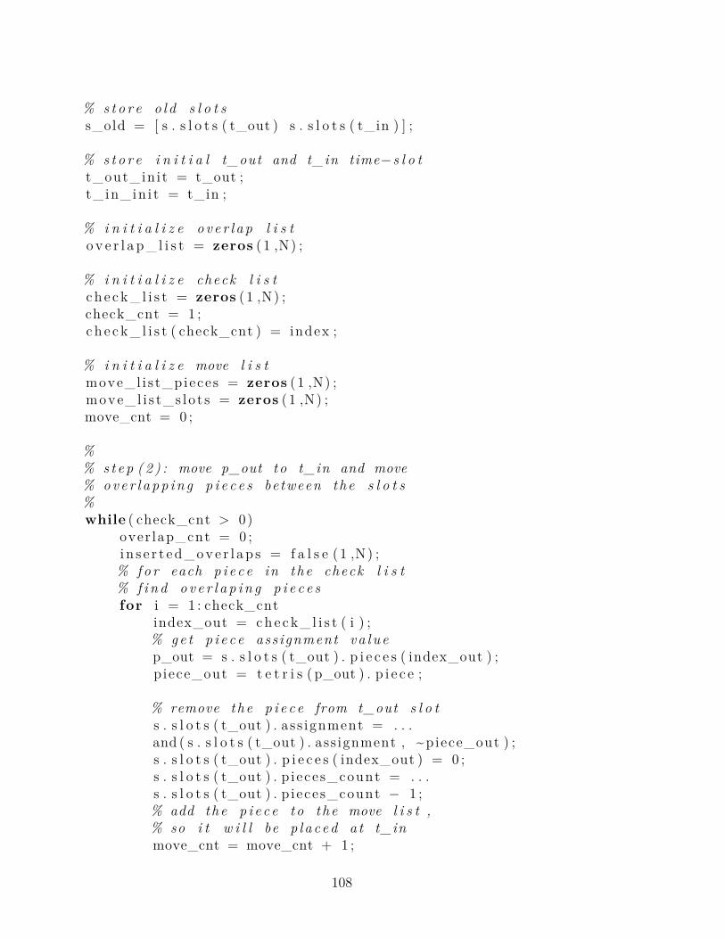
% s t o r e o l d s l o t ss_old = [ s . s l o t s ( t_out ) s . s l o t s ( t_in ) ] ;

% s t o r e i n i t i a l t_out and t_in time−s l o tt_out_in i t = t_out ;t_ in_in i t = t_in ;

% i n i t i a l i z e o v e r l a p l i s to v e r l a p _ l i s t = zeros ( 1 ,N) ;

% i n i t i a l i z e check l i s tc h e c k _ l i s t = zeros ( 1 ,N) ;check_cnt = 1 ;c h e c k _ l i s t ( check_cnt ) = index ;

% i n i t i a l i z e move l i s tmove_l i s t_pieces = zeros ( 1 ,N) ;move_l i s t_s lo t s = zeros ( 1 ,N) ;move_cnt = 0 ;

%% s t e p ( 2 ) : move p_out to t_in and move% o v e r l a p p i n g p i e c e s between the s l o t s%while ( check_cnt > 0)

over lap_cnt = 0 ;i n s e r t e d _ o v e r l a p s = f a l s e (1 ,N) ;% f o r each p i e c e in the check l i s t% f i n d o v e r l a p i n g p i e c e sfor i = 1 : check_cnt

index_out = c h e c k _ l i s t ( i ) ;% g e t p i e c e ass ignment va l u ep_out = s . s l o t s ( t_out ) . p i e c e s ( index_out ) ;p iece_out = t e t r i s ( p_out ) . p i e c e ;

% remove the p i e c e from t_out s l o ts . s l o t s ( t_out ) . ass ignment = . . .and ( s . s l o t s ( t_out ) . ass ignment , ~piece_out ) ;s . s l o t s ( t_out ) . p i e c e s ( index_out ) = 0 ;s . s l o t s ( t_out ) . p i eces_count = . . .s . s l o t s ( t_out ) . p i eces_count − 1 ;% add the p i e c e to the move l i s t ,% so i t w i l l be p l a c ed a t t_inmove_cnt = move_cnt + 1 ;

108

move_l i s t_pieces ( move_cnt ) = p_out ;move_l i s t_s lo t s ( move_cnt ) = t_in ;

% check f o r o v e r l a p between p i e c e s% in the check l i s t and t ho s e in% t_infor index_in = 1 : s . s l o t s ( t_in ) . p i eces_count

% g e t p i e c e d e t a l i s

p_in = s . s l o t s ( t_in ) . p i e c e s ( index_in ) ;p i e ce_in = t e t r i s ( p_in ) . p i e c e ;

% e v a l u a t e o v e r l a p p i n g between the two p i e c e sove r l ap = any ( and ( piece_in , p iece_out ) ) ;

% check i f t h e two p i e c e s o v e r l a pi f ( ove r l ap )

% add the index o f o v e r l a p p i n g% p i e c e to o v e r l a p l i s ti f ~ i n s e r t e d _ o v e r l a p s ( index_in )

i n s e r t e d _ o v e r l a p s ( index_in ) = t rue ;over lap_cnt = over lap_cnt + 1 ;o v e r l a p _ l i s t ( over lap_cnt ) = index_in ;

endend

endend% remove p i c e s from t_outr ema in ing_piece s = . . .find ( s . s l o t s ( t_out ) . p i e c e s > 0 ) ;n = s . s l o t s ( t_out ) . p i eces_count ;s . s l o t s ( t_out ) . p i e c e s ( 1 : n ) = . . .s . s l o t s ( t_out ) . p i e c e s ( r ema in ing_piece s ) ;s . s l o t s ( t_out ) . p i e c e s (n+1:end ) = 0 ;% update check l i s tc h e c k _ l i s t = o v e r l a p _ l i s t ;check_cnt = over lap_cnt ;

% swap the two time s l o t st = t_in ;t_in = t_out ;t_out = t ;

end

t_out = t_out_in i t ;

109

t_in = t_in_in i t ;

%% s t e p ( 3 ) : p l a c e p i e c e s in move l i s t% in t h e i r proper t ime s l o t s%% f o r each e lement in the move l i s tfor i = 1 : move_cnt

% g e t e lement d e t a l i sp = move_l i s t_pieces ( i ) ;t = move_l i s t_s lo t s ( i ) ;

% g e t the p i e c e d e t a i l s from the t e t r i s l i s tp i e c e = t e t r i s (p ) . p i e c e ;u = t e t r i s ( p ) . u s e r ;

% update u s e r s count i f t_out > Ti f t_out > T

i f t <= Ti f s . u s e r s (u ) == 0

s . users_count = s . users_count + 1 ;ends . u s e r s (u ) = s . u s e r s (u ) + 1 ;

elses . u s e r s (u ) = s . u s e r s (u ) − 1 ;i f s . u s e r s (u ) == 0

s . users_count = s . users_count − 1 ;end

endend

% p l a c e the p i e c es . s l o t s ( t ) . ass ignment = or ( p i ece , s . s l o t s ( t ) . ass ignment ) ;n = s . s l o t s ( t ) . p i eces_count ;s . s l o t s ( t ) . p i e c e s (n+1) = p ;s . s l o t s ( t ) . p i eces_count = n + 1 ;

end

% s t o r e new s l o t ss_new = [ s . s l o t s ( t_out ) s . s l o t s ( t_in ) ] ;

%% s t e p ( 4 ) : remove i n i t i a l t_out time−s l o t i f i t i s empty%i f s . s l o t s ( t_out ) . p i eces_count == 0

110

% remove empty t ime s l o t ss . s l o t s ( t_out ) = [ ] ;

end

f = c o s t _ p a r t i a l ( s_old , s_new , [ t_out t_in ] ) ;%di s p ( f ) ;%d i s p ( s . c o s t ) ;s . c o s t = s . c o s t + f ;%di s p ( s . c o s t ) ;end

%% Generate Random S o l u t i o nfunction s o l u t i o n = generate_random_solut ion ( )% genera t e a random s o l u t i o nglobal N M T t e t r i s A;

% g e t the t o t a l number o f p i e c e s in the t e t r i sn = length ( t e t r i s ) ;

% s o l u t i o n ( ass ignment ) s t r u c t u r e% ass ignment : l o g i c a l v e c t o r s i z e N% merges a l l p i e c e s i n t o to a time−s l o t% p i e c e s : i n t v e c t o r o f s i z e N% con ta in s the indec e s o f ass ignment p i e c e s% pieces_count : i n t% counts number o f used p i e c e s% use r s : i n t v e c t o r o f s i z e M% number o f ass i gnments to each user in the f i r s t T s l o t s% users_count : i n t% number o f u s e r s out o f M as s i gned to the f i r s t T s l o t s% c o s t : f l o a t% c o s t ( f i t n e s s ) o f t he s o l u t i o n

s o l u t i o n = s t r u c t ( ’ s l o t s ’ , repmat ( s t r u c t ( . . .’ ass ignment ’ , f a l s e ( 1 ,N) , . . .’ p i e c e s ’ , zeros ( 1 ,N) , . . .’ p i eces_count ’ , 0 ) , n∗A, 1 ) , . . .’ u s e r s ’ , zeros ( 1 ,M) , . . .’ users_count ’ , 0 , . . .’ c o s t ’ , 0 . 0 ) ;

% genera t e a random sample from the t e t r i st e t r i s_samp l e = randsample (n∗A, n∗A) ;t e t r i s_samp l e = mod( te t r i s_sample , n ) + 1 ;n = n ∗ A;

111

for i = 1 : length ( t e t r i s_samp l e )% g e t the index o f t he i ^ th sample ( p i e c e )index = te t r i s_samp l e ( i ) ;

% g e t the p i e c e from the t e t r i sp i e c e = t e t r i s ( index ) . p i e c e ;

for t = 1 : n% g e t the ass ignment in the t ^ th% s o l u t i o n ( t ^ th time−s l o t )ass ignment = s o l u t i o n . s l o t s ( t ) . ass ignment ;

% check o v e r l a p p i n g between the i ^ th% p i e c e and t ^ th time−s l o tove r l ap = and ( p i ece , ass ignment ) ;

% i f no over l ap , then do the f o l l o w i n gi f ~ ove r l ap

% merge the p i e c e wi th the% cur r en t ass ignments o l u t i o n . s l o t s ( t ) . ass ignment = . . .or ( p i ece , ass ignment ) ;

% add the index o f t he a s s i gned p i e c em = s o l u t i o n . s l o t s ( t ) . p i eces_count ;s o l u t i o n . s l o t s ( t ) . p i e c e s (m+1) = index ;s o l u t i o n . s l o t s ( t ) . p i eces_count = m + 1 ;break ;

endend

end

empty_slots = zeros (n , 1 ) ;k = 0 ;

for t = 1 : ni f s o l u t i o n . s l o t s ( t ) . p i eces_count == 0

% i f time−s l o t i s empty , then add i t to the empty−s l o t s l i s tk = k + 1 ;empty_slots ( k ) = t ;

endend

% d e l e t e empty time−s l o t s from the s o l u t i o n

112

s o l u t i o n . s l o t s ( empty_slots ( 1 : k ) ) = [ ] ;

for t = 1 :T% update u s e r s count f o r cur r en t time−s l o tfor i = 1 : s o l u t i o n . s l o t s ( t ) . p i eces_count

p = s o l u t i o n . s l o t s ( t ) . p i e c e s ( i ) ;u = t e t r i s ( p ) . u s e r ;i f s o l u t i o n . u s e r s (u ) == 0

s o l u t i o n . users_count = s o l u t i o n . users_count + 1 ;ends o l u t i o n . u s e r s (u ) = s o l u t i o n . u s e r s (u ) + 1 ;

endend

s o l u t i o n . c o s t = c o s t ( s o l u t i o n ) ;end

%% Compute S o l u t i o n Cost ( F i t n e s s )function f = c o s t _ p a r t i a l ( s_old , s_new , t )% computes the c o s t ( f i t n e s s ) o f a g i v en s o l u t i o nglobal t e t r i s M T h E R sigma h_sum ;

% i n i t i a l i z e channe l r e sponse s to be removed from t_out and t_inRHs = zeros (M, 2 ) ;RHi = ones (M, 2 ) . ∗ h_sum ;

% i n i t i a l i z e channe l r e sponse s to be added to t_out and t_inAHs = zeros (M, 2 ) ;AHi = ones (M, 2 ) . ∗ h_sum ;

% i n i t i a l i z e SINR to be removed from t_out and t_inRSINR = zeros (M, 2 ) ;

% i n i t i a l i z e SINR to be added to t_out and t_inASINR = zeros (M, 2 ) ;

% i n i t i a l i z e added /removed us e r susers_removed = f a l s e (M, 2 ) ;users_added = f a l s e (M, 2 ) ;

% compute channe l r e sponse s o f to% be removed and addedfor i = 1 : 2

% compute channe l r e sponse s to be% removed from t_out and t_in

113

for j = 1 : s_old ( i ) . p i eces_count% g e t p i e c e d e t a i l sp = s_old ( i ) . p i e c e s ( j ) ;p i e c e = t e t r i s (p ) . p i e c e ;u = t e t r i s ( p ) . u s e r ;

% update removed us e r susers_removed (u , i ) = t rue ;

% determine a c t i v e−l e d s in the% p i e c e ass ignmenta c t i v e _ l e d s = find ( p i e c e > 0 ) ;

% determine the sum o f channe l% re sponse s o f a c t i v e _ l e d shh = sum(h (u , a c t i v e _ l e d s ) ) ;

% remove channe l r e sponse s i f and on ly i f t <= Ti f t ( i ) <= T

RHs(u , i ) = RHs(u , i ) + hh ;RHi (u , i ) = RHi(u , i ) − hh ;

endend

% compute channe l r e sponse s to% be added to t_out and t_infor j = 1 : s_new ( i ) . p i eces_count

% g e t p i e c e d e t a i l sp = s_new ( i ) . p i e c e s ( j ) ;p i e c e = t e t r i s (p ) . p i e c e ;u = t e t r i s ( p ) . u s e r ;

% update added us e r susers_added (u , i ) = t rue ;

% determine a c t i v e−l e d s in the p i e c e ass ignmenta c t i v e _ l e d s = find ( p i e c e > 0 ) ;

% determine the sum o f channe l% re sponse s o f a c t i v e _ l e d shh = sum(h (u , a c t i v e _ l e d s ) ) ;

% add channe l r e sponse s i f and on ly i f t <= Ti f t ( i ) <= T

AHs(u , i ) = AHs(u , i ) + hh ;

114

AHi(u , i ) = AHi(u , i ) − hh ;end

endend

% compute incrementa l c o s tf = 0 ;for u = 1 :M

for i = 1 : 2% compute SINR to be removedi f users_removed (u , i )

RSINR(u , i ) = E ∗ R^2 ∗ RHs(u , i )^2 / . . .(E ∗ R^2 ∗ RHi(u , i )^2 + sigma ) ;

end% compute SINR to be addedi f users_added (u , i )

ASINR(u , i ) = E ∗ R^2 ∗ AHs(u , i )^2 / . . .(E ∗ R^2 ∗ AHi(u , i )^2 + sigma ) ;

endf = f + log2 (1 + ASINR(u , i ) ) − log2 (1 + RSINR(u , i ) ) ;

endend

%unass igned_users = M − t o t a l_a s s i gned_use r s ;%f = f − f /M ∗ unass igned_users ;

end

%% Compute S o l u t i o n Cost ( F i t n e s s )function f = c o s t _ f u l l ( s o l u t i o n )% computes the c o s t ( f i t n e s s ) o f a g i v en s o l u t i o nglobal t e t r i s M T h E R sigma h_sum ;

% i n i t i a l i z e SINRSINR = zeros (M,T) ;

s = s o l u t i o n ;

% i n i t i a l i z e channe l r e sponse s and% i n t e r f e r e n c e s f o r a l l u s e r shs = zeros (M,T) ;h i = ones (M,T) . ∗ h_sum ;

for t = 1 :T

115

% i n i t i a l i z e a c t i v e u s e r s in cur r en t t ime s l o tac t i v e_us e r s = f a l s e (1 ,M) ;

% compute channe l r e sponse s and i n t e r f e r e n c e% in the t ^ th time−s l o tfor i = 1 : s . s l o t s ( t ) . p i eces_count

% f o r each p i e c e p in the assignment ,% g e t t he user and ass ignment% va l u ep = s . s l o t s ( t ) . p i e c e s ( i ) ;u = t e t r i s ( p ) . u s e r ;p i e c e = t e t r i s (p ) . p i e c e ;

% update a c t i v e u s e r sac t i v e_us e r s (u ) = t rue ;

% determine a c t i v e−l e d s in% the p i e c e ass ignmenta c t i v e _ l e d s = find ( p i e c e > 0 ) ;

% determine the sum o f channe l% re sponse s o f a c t i v e _ l e d shh = sum(h (u , a c t i v e _ l e d s ) ) ;

% update channe l r e sponse s% and i n t e r f e r e n c e v a l u e shs (u , t ) = hs (u , t ) + hh ;h i (u , t ) = h i (u , t ) − hh ;

end

% compute SINR f o r u s e r s a s s i gned% in the t ^ th t ime s l o t sfor u = 1 :M

i f ac t i v e_us e r s (u )SINR(u , t ) = E ∗ R^2 ∗ hs (u , t )^2 / . . .(E ∗ R^2 ∗ h i (u , t )^2 + sigma ) ;

endend

end

% compute data r a t e per userDR = sum( log2 (1+SINR ) , 2 ) ;% compute the t o t a l data r a t ef = sum(DR, ’ a l l ’ ) ;%unass igned_users = M − t o t a l_a s s i gned_use r s ;

116

%f = f − f /M ∗ unass igned_users ;

end

%% Compute S o l u t i o n Cost ( F i t n e s s )function f = c o s t ( s o l u t i o n )% computes the c o s t ( f i t n e s s ) o f a g i v en s o l u t i o nglobal t e t r i s M T h E R sigma ;

% i n i t i a l i z e SINRSINR = zeros (M,T) ;

s = s o l u t i o n ;

a s s i gned_use r s = f a l s e (M, 1 ) ;t o t a l_as s i gned_use r s = 0 ;

for t = 1 :T% i n i t i a l i z e channe l r e sponse s and% i n t e r f e r e n c e in the t ^ th time−s l o ths = zeros (M, 1 ) ;h i = zeros (M, 1 ) ;

% g e t ass ignment in the t ^ th t ime s l o tass ignment = s . s l o t s ( t ) . ass ignment ;n = s . s l o t s ( t ) . p i eces_count ;p i e c e s = s . s l o t s ( t ) . p i e c e s ( 1 : n ) ;

% determine a c t i v e−l e d e s in the ass ignmenta c t i v e _ l e d s = find ( ass ignment > 0 ) ;

% determine us e r s in the ass ignmentu s e r s = f a l s e (1 ,M) ;

% i n i t i a l i z e channe l i n t e r f e r e n c e f o r%the u s e r s a s s i gned to a c t i v e−l e d s%h i ( u s e r s ) = sum( h ( users , a c t i v e _ l e d s ) , 2 ) ;

% compute channe l r e sponse s and%i n t e r f e r e n c e in the t ^ th time−s l o tfor p = p i e c e s

% f o r each p i e c e p in the assignment ,% g e t t he user and ass ignment% va l u e

117

use r = t e t r i s ( p ) . u s e r ;p i e c e = t e t r i s (p ) . p i e c e ;

i f ~ as s i gned_use r s ( u s e r )a s s i gned_use r s ( u s e r ) = t rue ;t o t a l_as s i gned_use r s = to ta l_as s i gned_use r s + 1 ;

end

u s e r s ( u s e r ) = t rue ;

% determine a c t i v e−l e d s in the p i e c e ass ignmentuse r_ac t iv e_ l eds = find ( p i e c e > 0 ) ;

% determine the sum o f channe l r e sponse s o f a c t i v e _ l e d sh_sum = sum(h ( user , u s e r_ac t iv e_ l eds ) ) ;

% update channe l r e sponse s and% i n t e r f e r e n c e v a l u e shs ( u s e r ) = hs ( u s e r ) + h_sum ;h i ( u s e r ) = h i ( u s e r ) − h_sum ;

endac t i v e_us e r s = find ( u s e r s ) ;h i ( a c t i v e_us e r s ) = h i ( a c t i v e_us e r s ) + . . .sum(h ( ac t ive_use r s , a c t i v e _ l e d s ) , 2 ) ;

% compute SINR f o r u s e r s a s s i gned% in the t ^ th t ime s l o t sfor use r = ac t i v e_us e r s

SINR( user , t ) = E ∗ R^2 ∗ hs ( u s e r )^2 / . . .(E ∗ R^2 ∗ h i ( u s e r )^2 + sigma ) ;

endend

% compute data r a t e per userDR = sum( log2 (1+SINR ) , 2 ) ;% compute the t o t a l data r a t ef = sum(DR, ’ a l l ’ ) ;end

%% Plo t Roomfunction f = plot_room ( )% p l o t s LEDs and use r s l o c a t i o n sglobal M PD LED L W;shgf = 0 ;

118

% show LEDs and use r s l o c a t i o n s on a% s c a t t e r p l o ts c a t t e r (LED( : , 1 ) , LED( : , 2 ) ) ;grid minor ;axis ( [ 0 L 0 W] )hold on ;s c a t t e r (PD( : , 1 ) , PD( : , 2 ) ) ;% l a b e l u s e r s on the p l o tu s e r s = ( 1 :M) ’ ;l a b e l s = num2str ( use r s , ’%d ’ ) ;text (PD( : , 1 ) , PD( : , 2 ) , l a b e l s , ’ h o r i z o n t a l ’ , . . .’ l e f t ’ , ’ v e r t i c a l ’ , ’ bottom ’ ) ;drawnow ;end

%% Plo t Assignmentfunction f = p l o t _ s o l u t i o n ( s o l u t i o n , . . .

CurFitness , Bes tF i tne s s , Tc )% show the users ’ ass ignment on heat−map p l o t% map the s o l u t i o n to an NxT matr ixmap = map_solution ( s o l u t i o n ) ;shgf = 0 ;% show the ass ignment on a heat−mapheatmap (map ) ;% d i s p l y t he cur r en t+b e s t f i t n e s s e s% and cur r en t tempera tures = sprintf ( ’ Current : ␣%f , ␣ Best : ␣%f , ␣Temp : ␣ . . .␣␣␣␣%f ’ , CurFitness , Bes tF i tne s s , Tc ) ;t i t l e ( s ) ;drawnow ;end%% Map S o l u t i o nfunction map = map_solution ( s o l u t i o n )% maps a s o l u t i o n o f a s t r i p s−game% problem to an NxT matr ixglobal N t e t r i s T;%T = l e n g t h ( s o l u t i o n ) ;map = zeros (N,T) ;for t = 1 :T

% g e t the number o f p i e c e s in the t ^ th time−s l o t%n = l e n g t h ( s o l u t i o n ( t ) . p i e c e s ) ;n = s o l u t i o n . s l o t s ( t ) . p i eces_count ;

% g e t a l l p i e c e s in the t ^ th time−s l o t

119

p i e c e s = s o l u t i o n . s l o t s ( t ) . p i e c e s ( 1 : n ) ;for k = 1 : n

% g e t index o f t he k^ th p i e c eindex = p i e c e s ( k ) ;% g e t user cor re spond ing to the k^ th p i e c euse r = t e t r i s ( index ) . u s e r ;% g e t the p i e c e va l u ep i e c e = t e t r i s ( index ) . p i e c e ;% g e t LEDs indec e s cor re spond ing to% the ass ignment r e p r e s e n t e d by% the p i e c e%l e d s = f i n d ( p i e c e == 1 ) ;% a s s i g n the LED and time s l o t% to the cur r en t usermap( p i e c e == 1 , t ) = use r ;

endendend

%% Compute T e t r i s P iece sfunction p i e c e s = compute_tet r i s_p iece s ( )% computes the op t ima l t e t r i s p i e c e s% f o r each user based on the number o f% time s l o t s a l l o c a t e d f o r each userglobal h M N A;

% user index : i n t e g e r number 1 . .M% t e t r i s p i e c e : l o g i c a l v e c t o r s i z e N% i n d i c a t e s LEDs are a s s i gned to userp i e c e s = s t r u c t ( ’ u s e r ’ , {} , ’ p i e c e ’ , { } ) ;

m = A;m = 1 ;

% s e t p i e c e s counterp i ece s_cnt = 1 ;for use r = 1 :M

% f i n d a c t i v e LEDs wi th channe l r e sponse s > 0a c t i v e _ l e d s = find (h ( user , : ) > 0 ) ;% f i n d channe l r e sponse s o f LEDs% as s i gned to the cur r en t userhu = h( user , a c t i v e _ l e d s ) ;% s o r t channe l r e sponse s in descend ing order[ ~ , I ] = sort (hu , ’ descend ’ ) ;% s o r t a c t i v e LEDs in descend ing order% o f t h e i r cahnne l r e sponse s

120

a c t i v e _ l e d s = a c t i v e _ l e d s ( I ) ;% f i n d number o f a c t i v e LEDsn = length ( a c t i v e _ l e d s ) ;

% genera t e p i e c e s o f i n d i v i d u a l% l e d s f o r the cur r en t userfor k = 1 : n

% g e t i ndec e s o f t he a c t i v e LEDsl e d = a c t i v e _ l e d s ( k ) ;% compute the p i e c ep i e c e = f a l s e (1 ,N) ;p i e c e ( l ed ) = t rue ;

% s t o r e m c o p i e s o f t he p i e c e in% the t e t r i s p i e c e s matr ixp = s t r u c t ( ’ u s e r ’ , user , ’ p i e c e ’ , p i e c e ) ;s t a r t _ p i e c e = p iece s_cnt ;end_piece = p iece s_cnt + m;p i e c e s ( s t a r t _ p i e c e : end_piece ) = p ;p i e ce s_cnt = piece s_cnt + m;

end

% genera t e p i e c e s wi th 2 or more l e d s% f o r the cur r en t userfor k = 2 : n

% g e t i ndec e s o f t he a c t i v e LEDsl e d s = a c t i v e _ l e d s ( 1 : k ) ;% compute the p i e c ep i e c e = f a l s e (1 ,N) ;p i e c e ( l e d s ) = t rue ;

% s t o r e m c o p i e s o f t he p i e c e in% the t e t r i s p i e c e s matr ixp = s t r u c t ( ’ u s e r ’ , user , ’ p i e c e ’ , p i e c e ) ;s t a r t _ p i e c e = p iece s_cnt ;end_piece = p iece s_cnt + m;p i e c e s ( s t a r t _ p i e c e : end_piece ) = p ;p i e ce s_cnt = piece s_cnt + m;

endendend

121

REFERENCES

[1] L. U. Khan, “Visible light communication: Applications, architecture,standardization and research challenges,” Digital Communications and Networks,vol. 3, no. 2, pp. 78 – 88, 2017. [Online]. Available: http://www.sciencedirect.com/science/article/pii/S2352864816300335

[2] “Cisco visual networking index: Global mobile data traffic forecast update, 2016-2021,” [Online]. Available: http://www.cisco.com/c/en/us/solutions/collateral/service-provider/visual-networking-index-vni/mobile-white-paper-c11-520862.html.

[3] J. G. Andrews, S. Buzzi, W. Choi, S. V. Hanly, A. Lozano, A. C. K. Soong, andJ. C. Zhang, “What will 5g be?” IEEE Journal on Selected Areas in Communi-cations, vol. 32, no. 6, pp. 1065–1082, June 2014.

[4] H. Haas, C. Chen, and D. O’Brien, “A guide to wireless networking by light,”Progress in Quantum Electronics, vol. 55, pp. 88 – 111, 2017. [Online]. Available:http://www.sciencedirect.com/science/article/pii/S0079672717300198

[5] H. H. Dobroslav Tsonev, Stefan Videv, “Light fidelity (li-fi): towards all-opticalnetworking,” in Proc. SPIE, vol. 9007, 2014, pp. 9007 – 9007 – 10.

[6] A. Jovicic, J. Li, and T. Richardson, “Visible light communication: opportunities,challenges and the path to market,” IEEE Communications Magazine, vol. 51,no. 12, pp. 26–32, December 2013.

[7] Z. Wang, Q. Wang, W. Huang, and Z. Xu, Introduction to Visible LightCommunications. IEEE, 2018. [Online]. Available: https://ieeexplore.ieee.org/xpl/articleDetails.jsp?arnumber=8268590

[8] “The ieee 802.15.13 multi-gigabit per second optical wireless communications taskgroup,” [Online]. Available: http://http://www.ieee802.org/15/pub/TG13.html.

[9] C. Medina, M. Zambrano Nuñez, and K. Navarro, “Led based visible light com-munication: Technology, applications and challenges – a survey,” vol. 8, pp.482–495, 09 2015.

[10] J. K. Member, J. M. Kahn, John, and R. Barry, “Wireless infrared communica-tions,” in Proc. Of the IEEE. Kluwer Academic Publishers, 1994, pp. 265–298.

122

[11] F. R. Gfeller and U. Bapst, “Wireless in-house data communication via diffuseinfrared radiation,” Proceedings of the IEEE, vol. 67, no. 11, pp. 1474–1486, Nov1979.

[12] C. Gussen, P. Diniz, M. Campos, W. Martins, F. Costa, and J. Gois, “A surveyof underwater wireless communication technologies,” Journal of Communicationand Information Systems, vol. 31, no. 1, Oct. 2016.

[13] Z. Zeng, S. Fu, H. Zhang, Y. Dong, and J. Cheng, “A survey of underwater opti-cal wireless communications,” IEEE Communications Surveys Tutorials, vol. 19,no. 1, pp. 204–238, Firstquarter 2017.

[14] E. M. Sozer, M. Stojanovic, and J. G. Proakis, “Underwater acoustic networks,”IEEE Journal of Oceanic Engineering, vol. 25, no. 1, pp. 72–83, Jan 2000.

[15] D. Pompili and I. F. Akyildiz, “Overview of networking protocols for underwaterwireless communications,” IEEE Communications Magazine, vol. 47, no. 1, pp.97–102, January 2009.

[16] J. Partan, J. Kurose, and B. N. Levine, “A survey of practical issues in underwaternetworks,” SIGMOBILE Mob. Comput. Commun. Rev., vol. 11, no. 4, pp. 23–33,oct 2007.

[17] K. Nakamura, I. Mizukoshi, and M. Hanawa, “Optical wireless transmission of405 nm, 1.45 gbit/s optical im/dd-ofdm signals through a 4.8 m underwaterchannel,” Opt. Express, vol. 23, no. 2, pp. 1558–1566, Jan 2015.

[18] C. Shen, Y. Guo, H. M. Oubei, T. K. Ng, G. Liu, K.-H. Park, K.-T. Ho, M.-S.Alouini, and B. S. Ooi, “20-meter underwater wireless optical communication linkwith 1.5 gbps data rate,” Opt. Express, vol. 24, no. 22, pp. 25 502–25 509, Oct2016.

[19] J. Xu, Y. Song, X. Yu, A. Lin, M. Kong, J. Han, and N. Deng, “Underwaterwireless transmission of high-speed qam-ofdm signals using a compact red-lightlaser,” Opt. Express, vol. 24, no. 8, pp. 8097–8109, Apr 2016.

[20] M. Kong, W. Lv, T. Ali, R. Sarwar, C. Yu, Y. Qiu, F. Qu, Z. Xu, J. Han, andJ. Xu, “10-m 9.51-gb/s rgb laser diodes-based wdm underwater wireless opticalcommunication,” Opt. Express, vol. 25, no. 17, pp. 20 829–20 834, Aug 2017.

[21] C. Gabriel, M. Khalighi, S. Bourennane, P. Leon, and V. Rigaud, “Channelmodeling for underwater optical communication,” in 2011 IEEE GLOBECOMWorkshops (GC Wkshps), Dec 2011, pp. 833–837.

[22] ——, “Monte-carlo-based channel characterization for underwater optical com-munication systems,” IEEE/OSA Journal of Optical Communications and Net-working, vol. 5, no. 1, pp. 1–12, Jan 2013.

123

[23] S. Tang, Y. Dong, and X. Zhang, “On path loss of nlos underwater wireless opticalcommunication links,” in 2013 MTS/IEEE OCEANS - Bergen, June 2013, pp.1–3.

[24] V. Guerra, C. Quintana, J. Rufo, J. Rabadan, and R. Perez-Jimenez, “Paralleliza-tion of a monte carlo ray tracing algorithm for channel modelling in underwaterwireless optical communications,” Procedia Technology, vol. 7, pp. 11 – 19, 2013,3rd Iberoamerican Conference on Electronics Engineering and Computer Science,CIIECC 2013.

[25] V. Guerra, O. El-Asmar, C. Suarez-Rodriguez, R. Perez-Jimenez, and J. M. Luna-Rivera, “Statistical study of the channel parameters in underwater wireless opticallinks,” in 3rd IEEE International Work-Conference on Bioinspired Intelligence,July 2014, pp. 124–127.

[26] W. Liu, D. Zou, P. Wang, Z. Xu, and L. Yang, “Wavelength dependent channelcharacterization for underwater optical wireless communications,” in 2014 IEEEInternational Conference on Signal Processing, Communications and Computing(ICSPCC), Aug 2014, pp. 895–899.

[27] Y. Dong, H. Zhang, and X. Zhang, “On impulse response modeling for underwaterwireless optical mimo links,” in 2014 IEEE/CIC International Conference onCommunications in China (ICCC), Oct 2014, pp. 151–155.

[28] F. Miramirkhani and M. Uysal, “Visible light communication channel modelingfor underwater environments with blocking and shadowing,” IEEE Access, vol. 6,pp. 1082–1090, 2018.

[29] A. Mora, D. Ganger, G. Wells, J. Zhang, X. Hu, C. Zhou, A. Richa, and C. Young-bull, “Ad-hoc multi-hop underwater optical network for deep ocean monitoring,”in 2013 OCEANS - San Diego, Sept 2013, pp. 1–5.

[30] F. Akhoundi, J. A. Salehi, and A. Tashakori, “Cellular underwater wireless op-tical cdma network: Performance analysis and implementation concepts,” IEEETransactions on Communications, vol. 63, no. 3, pp. 882–891, March 2015.

[31] M. V. Jamali, F. Akhoundi, and J. A. Salehi, “Performance characterization ofrelay-assisted wireless optical CDMA networks in turbulent underwater channel,”CoRR, vol. abs/1508.04030, 2015.

[32] M. V. Jamali, A. Chizari, and J. A. Salehi, “Performance analysis of multi-hopunderwater wireless optical communication systems,” IEEE Photonics TechnologyLetters, vol. 29, no. 5, pp. 462–465, March 2017.

[33] A. Tabeshnezhad and M. A. Pourmina, “Outage analysis of relay-assisted un-derwater wireless optical communication systems,” Optics Communications, vol.405, pp. 297 – 305, 2017.

124

[34] X. Ma, F. Yang, S. Liu, and J. Song, “Channel estimation for wideband un-derwater visible light communication: a compressive sensing perspective,” Opt.Express, vol. 26, no. 1, pp. 311–321, Jan 2018.

[35] C. D. Mobley, B. Gentili, H. R. Gordon, Z. Jin, G. W. Kattawar, A. Morel,P. Reinersman, K. Stamnes, and R. H. Stavn, “Comparison of numerical modelsfor computing underwater light fields,” Appl. Opt., vol. 32, no. 36, pp. 7484–7504,Dec 1993.

[36] J. Poliak, P. Pezzei, E. Leitgeb, and O. Wilfert, “Link budget for high-speedshort-distance wireless optical link,” in 2012 8th International Symposium onCommunication Systems, Networks Digital Signal Processing (CSNDSP), July2012, pp. 1–6.

[37] F. . U. M. Elamassie, Mohammed Miramirkhani, “Performance characterizationof underwater visible light communication,” IEEE Transactions on Communica-tions., 2018.

[38] M. Khalighi, T. Hamza, S. Bourennane, P. Léon, and J. Opderbecke, “Underwaterwireless optical communications using silicon photo-multipliers,” IEEE PhotonicsJournal, vol. 9, no. 4, pp. 1–10, Aug 2017.

[39] M. Kong, Y. Chen, R. Sarwar, B. Sun, Z. Xu, J. Han, J. Chen, H. Qin, and J. Xu,“Underwater wireless optical communication using an arrayed transmitter/re-ceiver and optical superimposition-based pam-4 signal,” Opt. Express, vol. 26,no. 3, pp. 3087–3097, Feb 2018.

[40] W. Liu, Z. Xu, and L. Yang, “Simo detection schemes for underwater opticalwireless communication under turbulence,” Photon. Res., vol. 3, no. 3, pp. 48–53, Jun 2015.

[41] F. Ahmed, S. Ali, and M. Jawaid, “A review of modulation schemes for visiblelight communication,” vol. 18, pp. 117–125, 02 2018.

[42] Y. Zhang, Z. Zhang, Z. Huang, H. Cai, L. Xia, and J. Zhao, “Apparent brightnessof leds under different dimming methods,” vol. 6841, 01 2008.

[43] S. Rajagopal, R. D. Roberts, and S. Lim, “Ieee 802.15.7 visible light commu-nication: modulation schemes and dimming support,” IEEE CommunicationsMagazine, vol. 50, no. 3, pp. 72–82, March 2012.

[44] H. Elgala, R. Mesleh, and H. Haas, “Indoor optical wireless communication:potential and state-of-the-art,” IEEE Communications Magazine, vol. 49, no. 9,pp. 56–62, September 2011.

[45] G. Miao, J. Zander, K. W. Sung, and S. Ben Slimane, Fundamentals of MobileData Networks. Cambridge University Press, 2016.

125

[46] A. M. Vegni and T. D. C. Little, “Handover in vlc systems with cooperatingmobile devices,” in 2012 International Conference on Computing, Networkingand Communications (ICNC), Jan 2012, pp. 126–130.

[47] T. Nguyen, M. Z. Chowdhury, and Y. M. Jang, “A novel link switching schemeusing pre-scanning and rss prediction in visible light communication networks,”EURASIP Journal on Wireless Communications and Networking, vol. 2013, no. 1,p. 293, Dec 2013.

[48] X. Bao, X. Zhu, T. Song, and Y. Ou, “Protocol design and capacity analysis inhybrid network of visible light communication and ofdma systems,” vol. 63, pp.1770–1778, 05 2014.

[49] E. Dinc, O. Ergul, and O. B. Akan, “Soft handover in ofdma based visible lightcommunication networks,” in 2015 IEEE 82nd Vehicular Technology Conference(VTC2015-Fall), Sept 2015, pp. 1–5.

[50] M. S. Demir, S. M. Sait, and M. Uysal, “Unified resource allocation and mobilitymanagement technique using particle swarm optimization for vlc networks,” IEEEPhotonics Journal, pp. 1–1, 2018.

[51] X. Li, R. Zhang, and L. Hanzo, “Cooperative load balancing in hybrid visiblelight communications and wifi,” IEEE Transactions on Communications, vol. 63,no. 4, pp. 1319–1329, April 2015.

[52] L. Li, Y. Zhang, B. Fan, and H. Tian, “Mobility-aware load balancing schemein hybrid vlc-lte networks,” IEEE Communications Letters, vol. 20, no. 11, pp.2276–2279, Nov 2016.

[53] Y. Wang and H. Haas, “Dynamic load balancing with handover in hybrid li-fi andwi-fi networks,” Journal of Lightwave Technology, vol. 33, no. 22, pp. 4671–4682,Nov 2015.

[54] Y. Wang, X. Wu, and H. Haas, “Load balancing game with shadowing effect forindoor hybrid lifi/rf networks,” IEEE Transactions on Wireless Communications,vol. 16, no. 4, pp. 2366–2378, April 2017.

[55] M. Obeed, A. M. Salhab, S. A. Zummo, and M. Alouini, “Joint optimizationof power allocation and load balancing for hybrid vlc/rf networks,” IEEE/OSAJournal of Optical Communications and Networking, vol. 10, no. 5, pp. 553–562,May 2018.

[56] B. Ghimire and H. Haas, “Resource allocation in optical wireless networks,” in2011 IEEE 22nd International Symposium on Personal, Indoor and Mobile RadioCommunications, Sept 2011, pp. 1061–1065.

[57] R. K. Mondal, M. Z. Chowdhury, N. Saha, and Y. M. Jang, “Interference-awareoptical resource allocation in visible light communication,” in 2012 InternationalConference on ICT Convergence (ICTC), Oct 2012, pp. 155–158.

126

[58] O. Babatundi, L. Qian, and J. Cheng, “Downlink scheduling in visible light com-munications,” in 2014 Sixth International Conference on Wireless Communica-tions and Signal Processing (WCSP), Oct 2014, pp. 1–6.

[59] Y. Tao, X. Liang, J. Wang, and C. Zhao, “Scheduling for indoor visiblelight communication based on graph theory,” Opt. Express, vol. 23, no. 3,pp. 2737–2752, Feb 2015. [Online]. Available: http://www.opticsexpress.org/abstract.cfm?URI=oe-23-3-2737

[60] F. Jin, X. Li, R. Zhang, C. Dong, and L. Hanzo, “Resource allocation under delay-guarantee constraints for visible-light communication,” IEEE Access, vol. 4, pp.7301–7312, 2016.

[61] X. Wu, M. Safari, and H. Haas, “Bidirectional allocation game in visible lightcommunications,” in 2016 IEEE 83rd Vehicular Technology Conference (VTCSpring), May 2016, pp. 1–5.

[62] D. Nguyen, N. Nguyen, N. Nguyen, and K. Spirinmanwat, “Light beam allocationalgorithm for eliminating interference in visible light communications,” in 2016International Conference on Advanced Technologies for Communications (ATC),Oct 2016, pp. 419–424.

[63] W. Wu, F. Zhou, and Q. Yang, “Dynamic network resource optimization in hybridvlc and radio frequency networks,” in 2017 International Conference on SelectedTopics in Mobile and Wireless Networking (MoWNeT), May 2017, pp. 1–7.

[64] F. Yunlong, L. Jianhui, L. Qing, and Z. Xiaoyi, “Downlink channel allocation ofvisible light communication network based on graph coloring and traffic fairness,”Procedia Computer Science, vol. 107, pp. 667 – 673, 2017, advances in Informationand Communication Technology: Proceedings of 7th International Congress ofInformation and Communication Technology (ICICT2017). [Online]. Available:http://www.sciencedirect.com/science/article/pii/S1877050917304210

[65] F. Seguel, A. D. Firoozabadi, P. Adasme, I. Soto, N. Krommenacker, andC. Azurdia-Meza, “A novel strategy for led re-utilization for visible lightcommunications,” Optik, vol. 151, pp. 88 – 97, 2017, optical WirelessCommunication Systems. [Online]. Available: http://www.sciencedirect.com/science/article/pii/S0030402617313347

[66] R. Jiang, Z. Wang, X. Zhu, and Q. Wang, “Interference-free led allocation forvisible light communications with fisheye lens,” Journal of Lightwave Technology,vol. 36, no. 3, pp. 626–636, Feb 2018.

[67] R. C. Kizilirmak, O. Narmanlioglu, and M. Uysal, “Centralized light access net-work (c-lian): A novel paradigm for next generation indoor vlc networks,” IEEEAccess, vol. 5, pp. 19 703–19 710, 2017.

127

[68] Y. S. Eroğlu, �. Güvenç, A. Şahin, Y. Yapıcı, N. Pala, and M. Yüksel, “Multi-element vlc networks: Led assignment, power control, and optimum combining,”IEEE Journal on Selected Areas in Communications, vol. 36, no. 1, pp. 121–135,Jan 2018.

[69] E. D. Demaine, S. Hohenberger, and D. Liben-Nowell, “Tetris is hard,even to approximate,” CoRR, vol. cs.CC/0210020, 2002. [Online]. Available:http://arxiv.org/abs/cs.CC/0210020

[70] S. Kirkpatrick, C. D. Gelatt, and M. P. Vecchi, “Optimization by simulatedannealing,” Science, vol. 220, no. 4598, pp. 671–680, 1983.

[71] V. Černý, “Thermodynamical approach to the traveling salesman problem: Anefficient simulation algorithm,” Journal of Optimization Theory and Applications,vol. P45, no. 1, pp. 41–51, Jan 1985.

[72] S. M. Sait and H. Youssef, Iterative Computer Algorithms with Applications inEngineering: Solving Combinatorial Optimization Problems, 1st ed. Los Alami-tos, CA, USA: IEEE Computer Society Press, 1999.

128

VITAE

• Name: Khaled Abdul-Aziz Eid Al-Utaibi

• Nationality: Saudi

• Date of Birth: 10/01/1393

• Email: alutaibi@uoh.edu.sa

• Permenant Address: Hail, Saudi Arabia

• Master of Science, Computer Engineering, 2002, King Fahd University ofPetroleum and Minerals, Dhahran, Saudi Arabia

• Bachelor of Science, Computer Engineering, 1997, King Fahd University ofPetroleum and Minerals, Dhahran, Saudi Arabia

129