Embed Size (px)
Citation preview

EVALUATION OF ABRASION RESISTANCE OF PIPE AND PIPE LINING MATERIALS
Final Report FHWA/CA/TL – CA01-0173
EA 680442
Glenn DeCou, P.E. Principal Investigator
Paul Davies, P.E. Co-Investigator
September, 2007
Department of Transportation
Office of Highway Drainage design, MS 28 1120 N Street
Sacramento, CA 95814

Caltrans abrasion test site at Shady Creek (Highway 49 crossing) photos: September 2001and 2005
(Cover photo: failed original pipe at outlet)

CONTENTS Page
1 SUMMARY 2 INTRODUCTION AND RESEARCH APPROACH
Agreements 3 TEST SITE LOCATION
General description Hydrology/Hydraulics
Rainfall Runoff Velocity Bedload Original Culvert
Pipe test panel concrete apron 17 MATERIALS 19 METHODOLOGY
Description 21 FINDINGS
Results and raw data Interpretation and contributing factors 40 APPLICATION Studies by others
Existing Caltrans guidance on abrasion Application
51 CONCLUSIONS 52 RECOMMENDATIONS 53 APPENDIXES
Appendix A Concrete test pad and panel installation photos
Appendix B Pipe test panel concrete frame construction details and photos
Appendix C Raw data charts and test panel photos Appendix D References Appendix E Proposed abrasion table for Design
Information Bulletin 83-01 and Table 854.3A of the Highway Design Manual
Appendix F Gage data for stream flow at Shady Creek and Jones Bar (Middle Fork Yuba River)

Office of State Highway Drainage Design
1
SUMMARY This project summarizes an evaluation of pipe material resistance to abrasion over a 5-year period (2001-2006) at a site known to be abrasive. The key focus of the project was to gather more information to compare against existing guidance to designers on evaluation of pipe material resistance to abrasion. To date, studies performed by others in laboratory settings have been limited and have not sufficiently reproduced real-world conditions for the entire range of pipe, and pipe lining products available today. See Appendix D. The objective of this research project was to evaluate various pipe and pipe liner products for their relative resistance to abrasion at a real-world abrasive test site. Results obtained from measurement and field observation will provide a major portion of the basis to update current design guidance and abrasion related input for Caltrans alternative pipe material service life predictions. Many existing culverts (primarily metal and concrete) that were placed during the height of the state highway building projects of the 1950’s and 60’s have now reached their service life expectancy and are in need of replacement or rehabilitation. Current guidance on abrasion resistance is inadequate because it is not specific enough and also does not cover the wide range of pipe and lining materials now available. This project evaluated the relative resistance to abrasion of seventeen different material types consisting of concrete, plastic, resin or metal along with various coatings and linings combined with metal. As a result of this study, and in the context of other information gathered outside of this study, modifications to Caltrans design guidance and service life prediction are recommended, including the following:
• New definitions for levels of abrasion
• A preliminary estimator of abrasion potential for material selection using bedload size, volume and velocity
• Predicted wear rates for each abrasion level
• New recommendations for allowable culvert and lining materials in abrasive
environments Overall, completion of this project represents a significant step forward for a better understanding of how to design of culverts and liners in abrasive environments.

Office of State Highway Drainage Design
2
INTRODUCTION AND RESEARCH APPROACH This abrasion research project was conducted by Caltrans headquarters Office of State Highway Drainage Design within the Division of Design in Sacramento. Pipe or liner manufacturers donated all test panels. The testing protocol and site to be used was presented and discussed with the manufacturers representatives at an initial meeting for their acceptance and agreement. It was explained that the abrasion test would be incorporated into a rehabilitation project of an existing 180-inch diameter, 260 foot long structural steel plate pipe (SSPP) located at a site known to be extremely abrasive in the Sierra foothills – see “Test Site Location” for details. The existing SSPP was concrete lined in the invert and had recently replaced a previous 1 gage SSPP that was chronically perforated in the invert after less than 20 years and structurally deformed. The rehabilitation project involved replacing the existing severely worn concrete invert lining in the replacement SSPP with a flat, 3/8th inch thick, steel plate. Agreements: It was agreed to use two test panels for each material being tested. These would be randomly placed in four rows formed within a 7-sack (class 1) concrete apron at the outlet of the SSPP. The agreed dimensions for each panel was a 1 square foot section (i.e., 12”x12”) taken from 48” diameter pipes or liners formed with a 24” radius. For each test panel provided, it was agreed to establish a uniform pattern and a fixed number of data points (9) for measuring thickness. The group decided to limit the testing to thickness measurement and visual inspection for all of the panels. Every sample would be measured at data points on a chosen pattern with a hand-held custom-made micrometer. Upon initial measurements and installation at the test site, it was agreed to remove the panels on an annual basis at the end of each rain season for measuring and then re-install them several months later - prior to the next rain season. After each year’s data collection was completed, an interim report would be circulated to industry representatives.

Office of State Highway Drainage Design
3
TEST SITE LOCATION General description The test site is located in Nevada County, Northern California, in the Sierra foothills at the Shady Creek crossing of Highway 49 (post mile 25.4) approximately 1000 feet west of the old Highway 49/Shady Creek bridge and 6 miles northwest of Nevada City - see map below.
Shady Creek is a perennial stream and tributary to the South Yuba River, which is part of the three-pronged Yuba River watershed, between the Feather and American rivers. The 12.3 square mile watershed is now recovering from major hydraulic gold mining activities that occurred in the mid 1800s to early 1900s. The Placer Diggins area is located within the upper watershed of Shady Creek (see map above) and comprises two former hydraulic mines, Cherokee Diggins, and North Columbia Diggins. Both heavily disturbed sites produce large volumes of angular quartz sand with small pebbles stored in low-gradient upland tributaries, which gets transported through the

Office of State Highway Drainage Design
4
test site. See pictures below.
Top left: Shady Creek 1 mile upstream. Top right: Channel downstream of test site. Middle (left): Malakoff Diggins (late 1800’s) - World’s largest Hydraulic mine located in adjacent basin to upper Shady Creek watershed. Middle (right): Bedload. Bottom (left): Malakoff Diggins today. Bottom (center): wear pattern on granite boulders 500 feet upstream. Bottom (right): severely worn concrete invert lining after two years inside culvert prior to placing steel plate invert protection.

Office of State Highway Drainage Design
5
The average elevation of the upstream watershed is approximately 2500 feet with upper peaks at elevation 3200 feet. The test site elevation at the culvert under highway 49 is approximately 1700 feet. It is located at a modified concrete apron at the pipe outlet and was incorporated into the rehabilitation project of an existing 180-inch diameter, 260 foot long, structural steel plate pipe. See pictures below:
Test panel installation Aerial view of pipe outlet, downstream channel and test site The average channel slope downstream of the Highway 49 crossing is approximately 0.013 feet/foot for approximately 5000 feet (see aerial view above). However, it is significantly steeper within just a few hundred feet upstream. See channel profile below. The culvert slope is 0.015 feet/foot.

Office of State Highway Drainage Design
6
The approach channel immediately upstream of the culvert entrance is skewed approximately 20 degrees. During winter flow events, as water enters the pipe, a large eddy current (vortex) several feet in diameter forms around the headwall on the left side and continues several feet into the pipe, which is invert-lined with a flat, 102 inch wide steel plate. See approach channel and culvert entrance pictures and notes below them:
Top left: Aerial view upstream of approach channel. Top right: Approach channel showing skew angle with culvert entrance. Bottom: Culvert entrance and vortex around left headwall. Note turbidity of water. It was speculated the vortex caused a significant reduction of sediment entering the left side of the culvert and over the concrete test pad at the outlet (see pictures on previous page).

Office of State Highway Drainage Design
7
As previously stated, Shady Creek is a perennial stream. However, during the summer and before the rain season begins in the fall, flows are reduced to a trickle through the culvert because a local rancher diverts flows upstream for irrigation. During the summer, the corrosive potential of the site is higher due to the lack of flow and local organic influences (note trees and surrounding cover in upstream pictures on previous page and forested upper watershed on page 4). Samples of bedload taken 50 feet upstream of the entrance in early November prior to the rain season indicated pH and minimum resistivity levels of 5.1 and 7,400, respectively. Results from pH and minimum resistivity tests of the soil and water taken for design are tabulated below: Ph Minimum Resistivity (R)-Ohm CM Soil Water Soil Water 5.8 6.8 10,300 15,100 6.0 6.9 8,300 14,700 Hydrology Rainfall: The mean annual precipitation within the 12.3 square mile watershed above the site at the Highway 49 crossing (elevation 1700 feet) varies from 40 to 55 inches, depending on elevation. The rain season typically begins in November and ends in May. During the five-year study period from 2001 to 2006 the annual rainfall totals recorded at local rain gages were as follows: Year: 2001/2 2002/3 2003/4 2004/5 2005/6 Reader Ranch: 43 in. 47 in. 32 in 45 in 51 in Nevada City: 55 in. 58 in. 20 in 80 in 86 in (el. 2279 ft) From November 2002 to the present, local rainfall totals have been recorded by the Reader Ranch gage, which is operated by the California Department of Forestry and located within a mile of the culvert at elevation 2025 feet. The Reader Ranch gage replaced a gage located at nearby Dorris Ranch (elevation 1968 feet). The complete Dorris Ranch historical record is shown below: Year Inches Year Inches 2001 24 1995 63 2000 41 1994 N/A 1999 38 1993 48 1998 57 1992 27 1997 41 1991 31 1996 N/A 1990 37 1989 30

Office of State Highway Drainage Design
8
A time of concentration (time runoff takes to travel from hydraulically most remote point in watershed to point of interest) of 2.16 hours was calculated by the District Hydraulics Branch for design. However, a stage gage placed inside the culvert during the study indicated the time of concentration was closer to 4 hours (see Page 11). The largest rainfall and runoff event recorded during the 5 year study occurred between December 31st, 2005, and January 1st, 2006, when over 4 inches of rain fell in less than 24 hours. By comparison, the highest rainfall total recorded locally prior to this event was on January 1st, 1997 when 3.76 inches were accumulated within 24 hours. During the most intense period of the 2005/6 storm, approximately 1 inch of rain fell within 120 minutes (see Reader Ranch rain gage plot below). From local rainfall intensity duration curves (see below), this storm could be considered to have a 50-year return period for intensity.
Rainfall Intensity vs Duration
0.00
0.50
1.00
1.50
2.00
2.50
3.00
3.50
4.00
4.50
5.00
5.500 10 20 30 40 50 60 70 80 90 100 110 120 130 140 150 160 170 180 190 200 210 220 230 240
Dur a t i on ( mi n)
2yrs Return Period 10yrs Return Period 25yrs Return Period 50yrs Return Period 100yrs Return Period
Reader Ranch rain gage plot from December 31st, 2005 to January 1st, 2006

Office of State Highway Drainage Design
9
Runoff: The District Hydraulics Branch reviewed the anticipated peak runoff flows to Design the Rock Slope Protection (RSP) for the culvert upgrade. In a Memorandum from Daniel Peterson, District 3 Hydraulics, to Frank Gould, Maintenance Engineering, dated June 29, 1999 (see Appendix I), it stated: “The original design (1975) for this culvert used a peak flow (100-year return period) of 2800 cubic feet per second (cfs) based on the Rational method. The peak flow was checked using the US Geological Survey (USGS) Regional Regression Equations, which resulted in a peak flow of 4300 cfs. The Soil Conservation Service Technical Release 55 (SCS TR-55) Method predicts a peak flow method of 4800 cfs.” The following runoff comparison between TR-55 and the Rational method was also included in the above-referenced 1999 District documentation for the culvert upgrade: Q-10 Q-10 Percent Q-100 Q-100 Percent Rational TR-55 Difference Rational TR-55 Difference Method Method Method Method 1,756 2,605 33% 3,111 4,815 35% Typically, the Rational Method is limited to drainage areas of 0.5 square miles in size or smaller as a hydrologic estimating tool. Additional discharge calculations were performed for this study independently of the above-referenced District calculations to obtain 2 and 5-year return frequency flood values (Q-2 and Q-5) as outlined in the Highway Design Manual (Index 854.3 (a)) to compare velocity for typical intermittent flow conditions with the velocities indicated in Table 854.3A. A stage gage placed inside the culvert by USGS (more details next page) provided sufficient data to be extrapolated for regression analyses. An independent analysis using USGS Regional Regression equations with updated rainfall data was also performed. The results are tabulated below. The TR-55 (District) values shown in the table were taken directly from the above-referenced District documentation. Return Estimated Discharge at Test Site Period LP III (17B) Regional
RegressionTR-55
(District) TR-55
(Tc=4 hours) Rational (District)
2 492 500 920 770 5 1018 1100 1400 10 1465 1500 2600 2000 1760 25 2136 2400 50 2707 3000
100 3337 4000 4800 3700 3100 500 5036 -
To supplement stage gage data at Shady Creek, discharge at the site during the five-year study period was estimated using basin transfer methodology with the closest DWR stream gage located approximately 2 miles away at Jones Bar on the South Fork

Office of State Highway Drainage Design
10
of the Yuba River near the confluence with Shady Creek. An extremely crude ratio of approximately 10:1 between sites was used. Standard basin transfer methods were not applicable due to significant variations in area (Yuba River watershed above Jones Bar is 308 square miles compared to 12.3 square miles at Shady Creek), elevation and snowmelt. A summary table of the peak flows recorded at Jones Bar during the five-year study period is presented below and an approximation of the Shady Creek peaks can be made by dividing the discharge values indicated in the table by a factor 10. The large event that occurred in May 2005 is an example where spring snowmelt was a major factor in the larger Yuba River basin. See Appendix F for a direct comparison of recorded flows at the two gages during a three-month period in 2004 and an enlarged summary table of peak flows at Jones Bar.
2001-2006
0
5000
10000
15000
20000
25000
30000
Oct Dec Dec Jan
Mar Dec Dec Jan
Mar AprMay Oct Dec Dec Ja
nFeb Oct Nov Ja
nFeb Mar Apr
May Nov Dec Dec Jan
Mar Mar AprMay
Month
Jone
s B
ar (c
fs)
2001-2006
At the Shady Creek site, using flows of 500 cfs (Q-2) and 1000 cfs (Q-5) with Manning’s equation, the associated water levels (stages) at the pipe outlet were estimated to be approximately 2.2 feet, and 3.7 feet, respectively. The stage gage at Shady Creek was funded and placed inside the culvert by USGS in cooperation with Caltrans and in conjunction with their study of sediment flows into Englebright Lake from the Yuba river system (including Shady Creek). For further information see: http://pubs.usgs.gov/sir/2005/5246/sir_2005-5246.pdf or http://pubs.usgs.gov/sir/2005/5246/Abstract.html For this study, the gage served the purpose of providing a better understanding of the watershed response to various storm events and its relationship with the Yuba River.

Office of State Highway Drainage Design
11
Within the five-year test period the stage gage was operational during the third rain season from August 2003 through May 2004. The third rain season was one of the two lowest years of rainfall during the five-year study. The average “peak” flow was around 92 cfs (see Page 13) with a stage of 0.8 feet. The fifth rain season was the highest, with an average “peak” flow of around 309 cfs (estimated using basin transfer) with a stage of 1.8 feet. Sample data of the third rain season from the Shady Creek gage is presented below along with an example plot of a single flood event. September 25, 2003 - January 30, 2004 Flow (cfs) V (fps) Hours Hours of flow greater than 0.4 ft >28 >8 186 Hours of flow greater than 0.5 ft >40 >9 118 Hours of flow greater than 0.6 ft >55 >10 68 January 2, 2004 – May 23, 2004 Flow (cfs) V (fps) Hours Hours of flow greater than 0.4 ft >28 >8 349 Hours of flow greater than 0.5 ft >40 >9 203 Hours of flow greater than 0.6 ft >55 >10 121 Hours of flow greater than 1.0 ft >130 >13.5 23 Total record from “all data” file Flow (cfs) V (fps) Hours Hours of flow greater than 0.4 ft >28 >8 710 Hours of flow greater than 0.5 ft >40 >9 461 Hours of flow greater than 0.6 ft >55 >10 257
Stage gage plot example for a single storm event that began at 0400 and ended around 1300 hours. From studying multiple events, it was determined that the actual time of concentration for the watershed was approximately 4 hours compared to an estimated time of 2.16 hours (from SCS TR-55).
Shady 2004 Feb 25
0
0.5
1
1.5
2
0 600 1200 1800 2400
time
dept
h (fe
et)
Series1
Office of State Highway Drainage Design
12
(Above left): Stage shown on stake approximating Q-2. (Above right):Typical winter storm flow level of 1-foot stage. As stated previously, the largest rainfall and runoff event recorded during the 5-year study occurred between December 31st, 2005, and January 1st, 2006. The stage gage at Shady Creek was not operational during this time, however, based on field review of the headwater pool high water marks at the culvert entrance shortly after the event occurred which indicated a headwater depth between 10-11 feet, the peak discharge was estimated using culvert hydraulics at approximately 1,200 cfs - between a 5 and10-year event (based on the Regional Regression method from page 11) with a flow depth inside the culvert of approximately 4.7 to 5.4 feet. The peak flow recorded at Jones Bar for that date was 28,000 cfs (see summary table). Other extremes documented for Jones Bar include 53,600 cfs on Dec. 22, 1964, and 30,300 cfs on Jan.1, 1997. For more detailed information see 1998 USGS Hydrologic data report website: http://ca.water.usgs.gov/archive/waterdata/98/11417500.html A local rancher of over fifty years described water levels on his property immediately downstream of the site as “one of the five highest” he had seen during his lifetime. Another long time resident of over sixty years who operates a small dam called “Shady Creek diversion” or sometimes known as the “Ponderosa dam” located upstream for the volunteer San Juan Ridge Water District, stated that the dam needed to be opened to release sediment, which rarely occurs, and also confirmed this was one of the top three or four flow events he had seen during his lifetime. Both of these accounts imply the December 2005 event may have been greater in magnitude than described above. Velocity: To estimate velocity at various flow depths, the FHWA software ‘HY-22 Open Channel Hydraulics’ (based on Manning’s equation) was used. At the lower depths where flow was contained within the steel plate trapezoidal channel, a trapezoidal cross section was used with a Manning’s roughness coefficient (n-value) of 0.012. The one-section model was calibrated with a field-measured velocity of 13.5 fps at a 1-foot flow depth. At higher stages when flow was above the 15-inch sides of the channel, to account for the influence of the corrugated structural steel plate pipe composite n-values ranging from 0.013 to 0.017 were assumed. In addition, for higher flow depths, a circular cross

Office of State Highway Drainage Design
13
section was compared. A velocity/discharge plot is presented on the next page. Note that the velocities in the plot for the 2 -5 year return frequency flood range (500-1000 cfs) used in context with HDM Table 854.3A are close to 20 feet per second (fps). As previously discussed, the largest flow event that occurred during the five-year study period was approximately 1200 cfs with an estimated peak velocity of 21-22 fps. See summary table below for approximate range of velocities for associated average peak, and peak discharge during each year of the 5-year study period.
Velocity/Discharge
0
200
400
600
800
1000
1200
1400
1600
0 5 10 15 20 25
Velocity (fps)
Dis
char
ge (c
fs)
Series1
( )Rain Year: (1) 2001/2 (2) 2002/3 (3) 2003/4 (4) 2004/5 (5) 2005/6
Ave. peak flow (cfs) 110 135 92 152 309 Ave. peak velocity (fps)
12.8 13.6 12 14.3 17.7
Peak flow (cfs) 300 500 300 1000 1200 Peak velocity (fps) 16.9 19.3 16.9 20.4 21.4
Bedload As stated previously, major hydraulic gold mining activities that occurred in the mid 1800s to early 1900s dramatically altered the upstream watershed and exposed large areas of gravel consisting of quartz and sand. During flow events, USGS sampled the sediment in Shady Creek at multiple locations including the old Highway 49 bridge approximately one thousand feet upstream as part of their study of sediment flows into Englebright Lake: http://pubs.usgs.gov/sir/2005/5246/Abstract.html. Caltrans also

Office of State Highway Drainage Design
14
performed independent sediment sampling for this study in accordance with California Test Methods 202 and 203. Both sets of results are plotted on the next page:
The Old Highway 49 sediment sampling (above) was performed on Feb. 25, 2004 during same event shown in stage gage plot example on page 13. (Below): Caltrans sampling results.
Soil Particle Size Distribution Curves (Caltrans convention larger sizes at left)
Test Method No.'s CA 202 and 203
0
10
20
30
40
50
60
70
80
90
100
0.0010.010.1110100
Particle Diameter (mm)
Perc
ent P
assi
ng
Site 9. Gower Wash at Zabriskie Point channel bottom Death Valley 09-Inyo-190S-1. Shady Creek channel bottom 50' u/s of culvert inlet 03-Nev-49 pm 25.1S-2. Shady Creek channel bottom 25' u/s of culvert inlet 03-Nev-49 pm 25.1
US Standard SieveOpenings (Inches)
US Standard Sieve Number Hydrometer
3/4"
1" 1/2"
3/8"
#4 #8 #16
#30
#50
#100
#200
5 μm
1 μm
2"4"
GRAVELSSILT
SANDSCoarse Fine Coarse Medium Fine
CLAY
SampleID:

Office of State Highway Drainage Design
15
From the plotted particle size distributions and the channel and bed-load photos on page 4, it can be seen that most of the larger quartz material ranges in size from 0.25 to 4 inches, while the remainder is mostly coarse grained sand of 0.1 mm (4 mils) and larger. Bed-load rating curves were developed by USGS using an empirical transport model for mixed-size sediment. Overall, the bed-load measurements by USGS agreed well with predicted curves; bed-load measurements were generally within the bounds of the bed-load rating curves (see below). Grain-size distributions for paired bed-load samples agreed well; sediment values were generally within 10 percent of each other. However, transport rates at the Old Hwy 49 site (shown in red) were generally over-predicted:
Even when over-prediction is accounted for, it can be seen that the two largest peak flow events listed on page 13 for rain years 4 and 5, likely produced significantly more bed-load than the peaks for the first three years. Owing to physical limitations of depth-integrating suspended-sediment samplers, samples by USGS were only collected from the water surface to within 0.3 ft of the streambed. Sampled sediment discharge consists of both fine material and bed material transported in suspension greater than 0.3 ft above the streambed. Unsampled sediment discharge (unsampled by the bed-load sampler) consists of both fine material and bed material transported in suspension less than 0.3 ft above the streambed and bed material transported as bed load. Total sediment discharge equates to the sum of sampled suspended-sediment discharge and estimated bed-load

Office of State Highway Drainage Design
16
discharge. The bed-load wear stain on the side of the trapezoidal channel near the outlet of the culvert adjacent to the test pad is located entirely within 0.3 ft above the invert in the “unsampled sediment discharge” zone. See picture below:
(Above): Bed-load wear stain on side of steel plate channel
Original Culvert A 180-inch, 1 gage SSPP was originally placed at this site in 1976. It was chronically perforated in the invert after less than 20 years and structurally deformed. See cover photo and pictures below.
Invert perforations in original culvert Sections of original culvert Pipe test panel concrete apron As discussed in the introduction, the pipe test panels were randomly placed in four rows formed within a 7-sack (class 1) concrete apron at the outlet of the SSPP being rehabilitated. The original plans called for an 8-ton RSP energy dissipator at the outlet embedded 12 feet below the original channel bed. The plans were modified to

Office of State Highway Drainage Design
17
incorporate a 1.25 ft (15 inch) minimum thickness, pipe test panel concrete apron placed at the same grade (0.015 ft/ft) as the culvert. During construction, more modifications to the design included concreting the 8-ton RSP, and the placement into the concrete apron of four pre-fabricated steel frames with welded half-inch bolts to facilitate test panel placement and removal. Six of the thirty-two (32) panels that were placed were too thick to be attached to the frames. For these, the concrete apron was formed to accommodate their individual dimensions and anchor bolts were placed. Each test row was spaced 22 inches (on center) leaving 10 inches of concrete between rows. Each row was recessed to enable the flow-line of each test panel to match adjacent panels and the upstream and downstream end of the concrete apron. None of the panels or apron were located inside the culvert, and therefore, there was no protection from UV exposure. See Appendix B for pipe test panel concrete apron and frame construction details and photos. MATERIALS Most of the alternative materials currently allowed by Caltrans and listed in Table 853.1A of the HDM were selected for this abrasion study. In addition, some new products were tested. Initially six (6) separate suppliers from industry donated a variety of products. Two more were added during the study. All of the pipe samples were taken from 48-inch diameter pipe and measured approximately one square foot (1 Sqft) in area. Holes were pre-drilled in each to accommodate half-inch bolts. A summary table listing pipe/lining materials and suppliers is presented on the next page. The two 4-inch concrete over galvanized CSP panels, were removed after the first year when it was discovered that the wrong concrete mix had been used. Individual panels made from basalt tile and calcium aluminate, were placed in the test locations originally reserved for the concrete paved CSP panels. Therefore, a total of eighteen different material types were supplied and tested. The mix design for the reinforced concrete pipe test panels indicated a minimum 28-day strength of 7000 psi (AASHTO Designation: M 170 requires 4000 psi for Classes I-IV and 6000 psi for Class V). The materials for the samples provided conformed to the requirements of Section 65, Reinforced Concrete Pipe, of the Standard Specifications. The plastic pipe panels donated were ribbed PVC and Type D corrugated HDPE. The materials for the samples provided conformed to the requirements of Section 64, Plastic Pipe, of the Standard Specifications. The steel pipe panels supplied were 16-gage (t=0.065”) and the aluminum panels were 12-gage (t=0.108”). The materials for the metal samples provided conformed to the requirements of Section 66, Corrugated Metal Pipe, of the Standard Specifications.

Office of State Highway Drainage Design
18
Pipe/liner Materials Summary Table: PIPE/LINING MATERIAL SUPPLIER Spec. Ref. 4” Concrete over galvanized CSP PC AASHTO M 36 Composite Steel Spiral Rib Pipe (CSSRP) PC AASHTO M 36 SSRP (Ribs at 7½ “ Pitch) PC AASHTO M 36 ASSRP (Ribs at 7½ “ Pitch) PC AASHTO M 36 SSRP with Polymerized Asphalt (Truflow TM) PC AASHTO M 36 Galvanized CSP – 2 2/3” x ½ Std. Corrugation PC AASHTO M 36 CASP – 2 2/3” x ½ Std. Corrugation PC AASHTO M 36 Galvanized CSP– 2 2/3” x ½ Std. Corrugation with Polymeric (Trenchcoat TM) Coating
PC AASHTO M 36
Galvanized CSP– 2 2/3” x ½ Std. Corrugation with Polymeric (Trenchcoat TM) Coating and Polymerized Asphalt (Truflow TM)
PC AASHTO M 36
Galvanized CSP– 2 2/3” x ½ Std. Corrugation and Polymerized Asphalt (Truflow TM)
PC AASHTO M 36
Galvanized CSP– 2 2/3” x ½ Std. Corrugation Bituminous Coated and Paved
PC AASHTO M 36
ASRP (Ribs at 7½ “ Pitch) Contech AASHTO M 196 Corrugated HDPE ADS AASHTO M 294 Ribbed PVC J-M Pipe AASHTO M 304 Cured in Place Pipe (CIPP) – Polyester Resin Insituform ASTM F 1216
& F 1743 Reinforced Concrete Pipe (RCP) CCP AASHTO M 170 Basalt Tile Abresist Calcium Aluminate mortar (SewperCoat TM) Lafarge Various ASTM LEGEND ASSRP - Aluminized Steel Spiral Rib Pipe SSRP - Steel Spiral Rib Pipe CSSRP - Composite Steel Spiral Rib (polymeric exterior, polyethylene interior liner) ASRP - Aluminum Spiral Rib Pipe CSP - Corrugated Steel Pipe CASP - Corrugated Aluminized Steel Pipe, Type 2 PC - Pacific Corrugated CCP - California Concrete Pipe Association The fused cast basalt (primarily volcanic rock) tile sample was donated by the Abresist Corporation and added in year 2. Its properties include a compressive strength of 71,000 psi, a hardness on the Mohs scale (diamond = 10) of up to 8, and chemically resistant to virtually all acids and alkalis. The Calcium Aluminate mortar panel was added in year 3. This product is used primarily to repair existing structures such as manholes and junction structures. The 28-day compressive strength is in excess of 10,000 psi. A small amount of Calcium Aluminate concrete (trade name Fondag TM) was used to repair parts of the pipe test panel concrete apron. This also had a 28-day compressive

Office of State Highway Drainage Design
19
strength in excess of 10,000 psi. No actual test panel was used and the only data collected was by visual inspection. METHODOLOGY General description The basic methodology for sampling and measuring that was employed is outlined under the introduction and research approach on page 2 – see “Agreements”. Generally, it was agreed to measure thickness and perform visual inspections on an annual basis. Thickness measurement: For each test panel provided, it was agreed to establish a uniform pattern and a set number of data points (9) for measuring thickness. The layout pattern and the custom built instrument used for measuring is shown below:
Typical layout of data measuring points. Mitutoyo Digimatic Scale Unit with Arrow represents flow direction. custom-built frame shown with largest test panel The x and y dimension for each data point was recorded. An attempt was made to locate data points on the leading edge of corrugated panels:
Black dots indicating data point locations on leading-
edge of corrugations

Office of State Highway Drainage Design
20
The custom-built measuring instrument shown on the previous page was capable of accurately measuring thickness to 0.001-inch (1 mil) increments. Visual inspection: For visual inspection and photo documentation, a steel grid frame made with 3-inch squares was used as a referencing tool to help document changes on each side of the panels and locate perforations or exposure of reinforcing steel (RCP panels).
Steel grid frame used for visual inspection and documentation General Procedure: As stated in the introduction, it was agreed with industry to remove the panels on an annual basis at the end of each rain season for measuring and then re-install them several months later. Therefore, the panels were not exposed to stream flow at all during the summer when the corrosive potential of the site is higher due to the lack of flow and local organic influences (see pH discussion under “General Description” on page 7). All of the test panels were measured and photographed the same way. Typically, two test panels represented each material type. However, there were some minor changes and additions made on an individual basis as test slots became vacant. See “Materials” – previous section. The four test rows were labeled A, B, C and D. Viewed downstream, row A was on the far right of the pipe test panel concrete apron (see Appendix A). The test panels that were mounted on the steel frames (see Appendix B) were placed in a random order, however, rows A and C, and rows B and D, contained like materials with the latter pair of rows having no corrugated profiles present. The three thickest panels that were too thick to be mounted on the steel frames were placed at the end of rows B and D in the same order and their placements were pre-formed into the concrete apron (see “Appendix B” for details). At the end of each rain season – usually by early June (see page 10 for more detail), the panels were removed from the site and taken back to the lab or office for measuring and photographing. Careful attention was made to label each panel and its orientation to flow for documentation purposes and to ensure the panels were returned

Office of State Highway Drainage Design
21
to their same spot and orientation as the original placement. Each year, besides the panels, the test site itself was also photographed to document changes to the concrete apron and channel upstream and downstream of the culvert. In addition, thickness measurements were taken on the steel plate invert inside the culvert. During the summer period when the panels were removed, manufacturers representatives were invited to perform a visual inspection of all the materials in addition to receiving an interim report of the latest data. Prior to each rain season – usually late September, the panels were reinstalled with new hardware (nuts, bolts and washers), and any necessary minor repairs to the concrete apron were made. FINDINGS Results and raw data See Appendix C for raw data charts and photos for each material. The original thicknesses measured at each data point upon installation in October 2001 are listed first followed below by successive years of wear at every data measuring point through 2006. Where there is no data shown for 2006, the panels were either completely destroyed or washed away by the numerous large events experienced during the fifth year of the study - see page 10 (“runoff”) and yearly photos documenting concrete apron in Appendix C. Presented on the following pages are wear rate summaries based on thickness measurements taken from all nine data points for each panel. See “Methodology” on page 19. See Appendix C for more detail. The wear rate summaries present both average and peak wear for each panel data. Peak wear rates (i.e., highest individual measured wear value for a given year) are shown in parenthesis. As discussed above, and in more detail in the runoff and velocity sections of this report, the final (fifth) year of this study was significantly different to the previous four years; eighteen (18) of the test panels were either completely destroyed or washed away. See summary table on page 13 for approximate range of velocities for associated average peak, and peak discharge during each year of the 5-year study period. 2001/2 and 2003/4 (Years 1 and 3) were found to be the lowest in terms of wear rates, peak flow, average peak and peak velocity. First perforation (fp) is indicated by the year it occurred and also shown in parenthesis. The (fp) calculation is based on the original thickness and assumes that first perforation occurred at the mid-point of the year. For example, if the first perforation occurred at some point during the third year, 65 mils (original thickness)/2.5 years = 26 mils/year and is denoted (fp 26). All wear rate values shown on the following pages are rounded to the nearest whole number.

Office of State Highway Drainage Design
22
Aluminum (t = 109 mils) Wear rate in mils/year Row C Row A 2001/2 (Year 1) 12 (32) 14 (22) 2002/3 (Year 2) 19 (35) 23 (36) 2003/4 (Year 3) 5 (11) 6 (17) (fp 43) 2004/5 (Year 4) 8 (20) 23 (50+) 2005/6 (Year 5) No data No data First perforation (fp) to row A panel occurred during year 3. No perforations to row C panel were observed through year 4. Both panels were destroyed during year 5. 1.2 in. (30 mm) Basalt tile (Abresist) Wear rate in mils/year Row D Row B 2001/2 (Year 1) (Installed Year 2) 2002/3 (Year 2) See Row B 9 (18) 2003/4 (Year 3) See Row B 1 (12) 2004/5 (Year 4) 14 (26) See Row D* 2005/6 (Year 5) 5 (16) See Row D *Panel moved to row D Cured-in-place pipe Wear rate in mils/year (Polyester resin t = 0.5 in.) Row D Row B 2001/2 (Year 1) 4 (13) 8 (17) 2002/3 (Year 2) 1 (8) 58 (82) 2003/4 (Year 3) 5 (9) 9 (21) 2004/5 (Year 4) 2 (12) 26 (36) 2005/6 (Year 5) 47 (54) No data HDPE Wear rate in mils/year (Inner liner t =180 mils) Row D Row B 2001/2 (Year 1) 7 (41) 15 (42) 2002/3 (Year 2) 14 (18) 58 (108) 2003/4 (Year 3) 11 (27) 43 (108) 2004/5 (Year 4) 7 (20) 12 (21) (fp 51) 2005/6 (Year 5) 13 (43) 50 (92) (Limited data) PVC (t =210 mils) Wear rate in mils/year Row D Row B 2001/2 (Year 1) 0 (2) 7 (13) 2002/3 (Year 2) 2 (6) 27 (39) 2003/4 (Year 3) 3 (4) 10 (13) 2004/5 (Year 4) 5 (10) 9 (16) 2005/6 (Year 5) No data - (74) Limited data

Office of State Highway Drainage Design
23
RCP Wear rate in mils/year (t = 5.8 in & 6 in.) Row D** Row B 2001/2 (Year 1) 23 (45) 221 (372) 2002/3 (Year 2) 79* (265) 1007* (1,358) 2003/4 (Year 3) 163 (622) 277 (617) 2004/5 (Year 4) 80 (254) 293 (410) 2005/6 (Year 5) 1,106 (1,680) No data *Steel reinforcement exposure (1.6”+/- concrete cover) occurred to both panels during year 2. ** Panel impacted during Year 1 as a result of defective material being placed on test panel immediately upstream. CSSRP (75 mil Polyethylene/ .064” steel) Wear rate in mils/year Row D Row B 2001/2 (Year 1) 1 (5) 4 (8) 2002/3 (Year 2) 2 (10) 15 (25) (fp liner* 50) 2003/4 (Year 3) 6 (8) 8 (16) 2003/4 (Year 4) 4 (11) 10 (17) 2005/6 (Year 5) 11 (15) (fp* 17) 64 (65) (fp steel) Limited data * (fp)refers to first perforation of polyethylene liner, not steel (see photos in Appendix C) Year 5, row B; only three data points remained. Measured wear to exposed steel was approximately 50 mils. Year 5, row D; Liner delaminated, perforated, and folded over deflecting flow. CSP with Bituminous Coating and Paved Wear rate in mils/year (t = 250 - 350 mils)**
Row C Row A 2001/2 (Year 1) 107 (178) 29 (91) 2002/3 (Year 2) 46 (110) (fp 43*) 133 (201) 2003/4 (Year 3) 15 (23) 41 (84) 2004/5 (Year 4) 8 (59) 40 (138) (fp 18*) 2005/6 (Year 5) No data 83 (>139) * Total thickness including variable coating on both sides and 0.064” steel First perforation (fp) to row A panel occurred during year 4, and year 2 for row C, which was destroyed during year 5. *Wear rate for fp is for 16 gage steel only and ignores the coating. CSP with Polymerized Asphalt (Truflow TM) Wear rate in mils/year (t = 140 – 180 mils)
Row C Row A 2001/2 (Year 1) 45 (61) 49 (75) 2002/3 (Year 2) 21 (37) 19 (36) 2003/4 (Year 3) 25 (44) 6 (17) 2004/5 (Year 4) 3 (9) 16 (27) (fp 18*) 2005/6 (Year 5) 13 (25) (fp 14*) 13 (21) First perforation (fp) to row A panel occurred during year 4, and year 5 for row C. *Wear rates for fp is for 16 gage steel only and ignores the coating. Actual wear rates for steel during year 5 are assumed to be higher than maximum values shown in parenthesis. ** Total thickness including variable coating on both sides and 0.064” steel

Office of State Highway Drainage Design
24
SSRP with Polymerized Asphalt (Truflow TM) Wear rate in mils/year (t = 150 – 200 mils)**
Row C Row A 2001/2 (Year 1) 36 (70) 30 (54) 2002/3 (Year 2) 20 (42) 19 (35) 2003/4 (Year 3) 21 (33) 3 (12) 2004/5 (Year 4) 6 (20) 15 (24) (fp 18*) 2005/6 (Year 5) No data No data ** Total thickness including variable coating on both sides and 0.064” steel First perforation (fp) to row A panel occurred during year 4. Both panels were destroyed in year 5. *Wear rate for fp is for 16 gage steel only and ignores the coating. CSP (10 mil Polymeric (Trenchcoat TM) Sheet Coating/ 0.064” steel)
Wear rate in mils/year Row C Row A
2001/2 (Year 1) 17 (23) 16 (22) 2002/3 (Year 2) 13 (28) 9 (26) 2003/4 (Year 3) 7 (13) 8 (28) 2004/5 (Year 4) 3 (5) 7 (15) 2005/6 (Year 5) 7 (19) (fp 14*) 4 (17) (fp 14*) First perforation (fp) to both panels occurred during year 5.* Wear rate for fp is for 16 gage steel only and ignores the coating. CSP with 10 mil Polymeric (Trenchcoat TM) & Polymerized Asphalt (Truflow TM) Coating (t = 170 – 230 mils)**
Wear rate in mils/year Row C Row A
2001/2 (Year 1) 33 (53) 54 (66) 2002/3 (Year 2) 58 (78) 30 (56) 2003/4 (Year 3) 24 (40) 12 (28) 2004/5 (Year 4) 10 (22) 11 (23) 2005/6 (Year 5) 24 (41) (fp 14*) 24 (48) (fp 14*) ** t= variable polymerized asphalt and 10 mil polymeric coating on both sides and 0.064” steel First perforation (fp) to both panels occurred during year 5. *Wear rate for fp is for 16 gage steel only and ignores the coating. CASP (t = 60 mils) Wear rate in mils/year
Row C Row A 2001/2 (Year 1) 5 (12) 1 (6) 2002/3 (Year 2) 15 (24) 11 (17) 2003/4 (Year 3) 5 (10) (fp 26) 3 (11) (fp 26) 2004/5 (Year 4) 2 (3) 7 (10) 2005/6 (Year 5) 11* (>25) 3* (>38) First perforation (fp) to both panels occurred during year 3. *Very limited data available for year 5.

Office of State Highway Drainage Design
25
ASSRP Wear rate in mils/year (t = 60-65 mils) Row D Row B 2001/2 (Year 1) 2 (5) 0 (3) 2002/3 (Year 2) 1 (2) 6 (10) 2003/4 (Year 3) 3 (5) 5 (13) 2003/4 (Year 4) 4 (6) 5 (12) 2005/6 (Year 5) No data No data No perforations to either panel through year 4. Both panels destroyed during year 5. CSP (t = 60 mils) Wear rate in mils/year
Row C Row A 2001/2 (Year 1) 6 (15) 2 (4) 2002/3 (Year 2) 8 (22) 6 (8) 2003/4 (Year 3) 5 (13) (fp 26) 6 (19) 2004/5 (Year 4) 11 (20) 9 (16) (fp 18) 2005/6 (Year 5) - (>20) - (>32) First perforation (fp) occurred during year 3 in Row C, and year 4 in row A. Limited data available for year 5. SSRP (t = 60-64 mils) Wear rate in mils/year Row D Row B 2001/2 (Year 1) 1 (2) 2 (10) 2002/3 (Year 2) 1 (2) 22 (28) 2003/4 (Year 3) 6 (10) 6 (>27) 2003/4 (Year 4) 3 (8) 8 (29) (fp 18) 2005/6 (Year 5) 8 (13) (fp 14) No data First perforation (fp) occurred during year 4 in row B. Limited data available for year 5 for row B. Pinhole first perforation (fp) occurred during year 5 in row D. Comparative peak wear rates for uncoated steel panels by profile type: Row D (SRP) Rows A-C (SRP) Rows A-C (Corrugated) 2001/4 (Years 1-4) 2-10 mils/year 3-29 mils/year 3-26 mils/year 2005/6 (Year 5) 14 mils/year No data >38 mils/year Peak wear rates to 3/8 in. (9.5 mm) A572 Grade 50 Steel plate invert repair (8.5 ft. x 267 ft.) * Row D Rows A-C 2001 thru 2005 4-6 mils/year 7-12 mils/year 2006 7-20 mils/year 25-50 mils/year *See Appendix C for detailed cross sections and profile.

Office of State Highway Drainage Design
26
Calcium Aluminate Mortar (SewperCoat TM) variable thickness overlay Row B 2004 thru 2005 39 (120 leading edge, 13 elsewhere) 2006 No data Another Calcium Aluminate Concrete product (Fondag TN) was used to make repairs to the concrete apron in the vicinity of rows A-C after year 4. See photos in Appendix C. Relative Peak Annual Wear Rates – Summary Presented below and on the next page are two charts summarizing selected peak annual wear rates for rows A-C and row D. Most of the materials are presented in these charts except RCP due to scaling (in Appendix C, RCP is the only material with its wear rate presented in inches rather than mils). Except for the polyethylene liner for CSSRP, none of the coatings for steel pipe are presented in these two charts, i.e., bituminous, asphaltic, polymeric or polymerized asphalt etc. Refer to the end of the next section (“Interpretation…”) for a discussion on their influence.
Selected Peak Annual Wear Rates (Rows A-C)
0
20
40
60
80
100
120
140
Steel P
late (
A-C)
SSRP (B)
ASRP ( B)
CSP (A)
CSP (C)
CASP (A)
CASP (C)
Aluminu
m SRP (A)
Aluminu
m SRP (C)
CSSRP (B)
CIPP (B)
PVC (B)
HDPE (B)
Basalt
Tile (B
)
Calcium
Alum
inate
(B)
Material (Row of placement)
Wea
r Rat
e (m
ils/y
ear)
2001-20052006

Office of State Highway Drainage Design
27
Selected Peak Annual Wear Rates (Row D)
0
10
20
30
40
50
60
Steel plate SSRP ASSRP CSSRP CIPP PVC HDPE Basalt Tile
Material
Wea
r Rat
e (m
ils/y
ear)
2001-2005
2006
Interpretation and contributing factors As described under ‘Test Site Location’, this site is considered extremely aggressive from an abrasion standpoint, particularly when compared with the abrasion potential for the smaller watersheds typically associated with 48-inch diameter pipes. However, it should be understood that the same materials that were used for this study, are used on both larger and smaller diameter culverts. As described earlier, the original 180-inch diameter, 1-gage SSPP perforated in less than 20 years of its intended 50-year maintenance free service life. In the summer of 2006, approximately thirty other steel pipe sites located in abrasive environments at various locations in California were reviewed for comparison with steel wear rates generated from the Shady Creek site. Almost every site produced significantly lower wear rates. See “Studies by others”. Due to the wide, flat steel plated invert placed in the replacement 180-inch diameter SSPP in 2001, the flow depths (generally less than one foot) and velocity (generally less than fifteen feet per second) generated for most events are comparable with those generated by many 48 inch diameter culverts elsewhere. However, several closely linked factors are dramatically different which include; the watershed size of 12.3 square miles, and both the volume and availability of bed-load within the watershed. Even for similar sized watersheds, the volume of bed-load transported through this site as a result of the historic mining activities is considered extreme and not typical of the volumes transported at most culvert locations elsewhere in California. See bed-load transport rates on page 15.

Office of State Highway Drainage Design
28
Although the bed-load volumes are considered to be extreme, they were not uniformly distributed across the entire cross section(s) of the steel plate invert lining inside the 180-inch SSPP and the concrete test panel apron. As explained in detail under ‘Test Site Location’, the combined geometry of the approach angle of the upstream channel and headwall created a large vortex in the flow at the entrance to the pipe potentially channeling large amounts of bed-load away from the left side of the smooth, flat invert and concrete test panel apron. This may explain how both the concrete test panel apron and panels in row D, as well as the steel plate invert on the left side experienced significantly less wear than the center and right side. See plots of steel plate thicknesses at the end of Appendix C. From an environmental standpoint, because the samples used were segmented panels rather than full pipe sections, except for the summer months they were continuously exposed to sunlight and UV rays, unlike most buried pipe installations (except at the ends). However, the effect of prolonged UV exposure to the panels most prone to potential UV degradation (PVC, HDPE, CSSRP, bituminous, polymeric and polymerized asphalt coatings) was immeasurable – particularly for the coated corrugated metal samples where most of the coatings on the leading edges of corrugations where data points were located were completely worn away during the first year exposing the steel. During the summer months when the corrosive potential of the site is higher due to the lack of flow and local organic influences, the panels were completely removed from the site for data collection. Prior to measuring, and at the same time the panels were removed, the panels were cleaned which removed some rust nodules. Even though all of the panels were cleaned, due to the sensitivity of the measuring device used, and as a result of the effects of corrosion, or other minor deposits on the wearing surface – along with wear pattern influences, some data points occasionally produced increases in thickness recordings. It should be noted that the estimated and measured wear rates for exposed steel include an assumed additional loss of 2 mils/year due to the effects of corrosion. Given the parameters for acidity and minimum resistivity for this site that are outlined on page 7, and using the Highway Design Manual Figure 854.3C (Chart for Estimating Years to Perforation of Steel Culverts), for a 16 gage (64 mils) pipe it is estimated that there would be 22 years to perforation. Therefore, the annual loss rate due to the effects of corrosion could be as high as 3 mils/year. However, as stated previously, the test panels were removed from the site during the summer months likely offsetting some of the corrosion losses. Therefore, the assumed loss rate selected for the effects of corrosion was 2 mils/year. Another effect of the samples being segmented was the influence of wear at the leading edges, which may have resulted in deflecting flows or premature de-lamination of some coatings. Presented on the following pages for each material is an interpretation of the raw data provided in Appendix C and the averaged and peak wear rates listed in the previous section under ‘Findings’. It should be noted that regardless of the wear rates recorded at the data points, by Caltrans standards for flexible pipe (i.e., metal or plastic), first perforation signal the end of maintenance free service. Therefore, the (calculated) wear
Office of State Highway Drainage Design
29
rate of the first perforation observed is as important or more significant than the wear rates recorded at the nine data points. Similarly, for the reinforced concrete samples, first exposure of steel reinforcement is significant. However, end of maintenance free service life does not constitute failure; although it was impossible to determine the actual rate of wear to most of the protective coatings for the steel panels, it is significant to note that after the large events of the fifth year, even though all of the remaining steel panels were perforated to some degree, in the three most abrasive rows, only the panels with some type of coating on the back side remained mostly intact and were not destroyed. Aluminum (spiral rib): Both panels were destroyed during year 5. The averaged wear rates from the data points were very similar during each of the first four years. However, significantly, during year 3 the panel in row A perforated along the leading edge of the rib for several inches in a thin line. The annual wear rate leading up to first perforation was 43 mils/year which was approximately 2.5 times higher than the averaged annual rates of 17 mils/year from the data points in the same panel (assuming first perforation occurred mid way through year 3). There were no perforations observed anywhere on the panel in row C which also experienced slightly lower wear rates than the panel in row A. By year 2, both panels were significantly worn at the leading edge. It is undetermined why the panel in row C seemingly “outperformed” the counterpart in row A. One explanation could be the placement within respective rows; the panel in row A was the very first in the row with the smooth metal plate directly upstream. The panel in row C was third back with a corrugated metal sample directly upstream, which may have deflected some flow offering limited protection. See Appendix A. In row C, in a single year, the maximum annual wear rate recorded was 35 mils/year compared with an averaged annual rate of 19 mils/year for the same year (year 2). During the same time period, compared to the uncoated corrugated steel panels in the same rows, the Aluminum panels wore 2-3 times faster in row A, and 1.5-2 times faster in row C. A comparison between the peak annual wear rates for both panels with the uncoated spiral rib steel panels also indicated that under similar conditions Aluminum abrades approximately 2-3 times faster than steel. Caltrans current design guidance in the Highway Design Manual states that under similar conditions Aluminum abrades approximately three times faster than steel. Basalt Tile (trade name “Abresist): The single Basalt tile composite test panel was added to row B after the first year of the study. After two years of virtually no wear in relation to its total thickness of 2 inches (1.2 inch (30 mm) tile, grout and 3/16 inch steel frame) except some minor beveling along the leading edge, it was moved to row D to incorporate another new product in the “aggressive” row B. Due to corrosion by-products that appeared on the steel casing for the sample, and the minimal abrasive wear of the tile, accurate measurements were

Office of State Highway Drainage Design
30
difficult to obtain and at times the readings indicated a slight increase in total thickness. Based on the data collected, the average wear was approximately 7 mils/year. However, after Year 5 – by far the most extreme from an abrasion standpoint, approximately 5 mils of (average) wear was recorded between the nine data points indicating that some of the previous years readings may have been erroneous and/or skewed by residual corrosion by-products on the steel frame the basalt tiles were encased in (see photos in Appendix C). The maximum annual wear rate recorded at a single data point during the extreme Year 5 was 16 mils/year compared with 20 mils/year to the steel plate inside the culvert near row D (towards the center, the wear to the steel was 50 mils/year). Overall, the basalt tile sample performed extremely well, and could meet a maintenance free service life of 50 years at this site. However, it should be noted that some of the other materials provided are available in increased thicknesses and could also meet the service life at this site (e.g. solid wall HDPE and steel plate). Cured in place pipe (CIPP) made from polyester resin: The smooth profile CIPP samples, along with the steel plate inside the culvert provide an excellent reflection of the previously discussed variable abrasion potential across the concrete apron from left to right (viewed downstream) and also of the variation in wear rate between the individual years of the study as a result the number and size of the storms and associated velocity (see pages 10 and 13). The CIPP panel in the more benign row D (where it is assumed that less bed-load was present) survived all five years of the test with virtually no wear during the first four years (1- 5 mils/year average wear recorded). However, year 5 produced a maximum of 54 mils of wear in one season and completely destroyed the panel in row B (or at the very least its anchorage – see pictures in Appendix C). With the smooth profile, the wear was distributed evenly to both panels. By the end of year 2, the leading edge to the panel in row B was significantly worn. This did not occur until year 5 in row D. The variability of the storm seasons for the first four years of this study is reflected best by the wear rates seen in the row B sample: Years 1 and 3 were very similar in terms of average wear compared to average and peak velocity generated during the same years:
Wear rate in mils/year Velocity (fps)
Row D Row B Ave Peak Vel. Peak Vel. 2001/2 (Year 1) 4 (13) 8 (17) 12.8 16.9 2002/3 (Year 2) 1 (8) 58 (82) 13.6 19.3 2003/4 (Year 3) 5 (9) 9 (21) 12 16.9 2004/5 (Year 4) 2 (12) 26 (36) 14.3 20.4 2005/6 (Year 5) 47 (54) No data 17.7 21.4

Office of State Highway Drainage Design
31
High Density Polyethylene (HDPE) - Type D Corrugated The values in the thickness charts in Appendix C represent the assumed thickness of the inner liner. Type D panels are of the closed cell type with an inner and outer wall. The total thickness of each 48-inch diameter sample was close to 2.5 inches. The high sensitivity of the measuring instrument made the samples difficult to measure due to the ridges and grooves on the exterior. This may explain some of the apparent increases documented at various data points. Except for the first year of the study, the recorded wear rates of the two HDPE samples also reflected the previously discussed varied abrasion potential across the concrete test apron. During years 2 through 5 the relative wear rate in row B was more than four times the rate in row D. When comparing the recorded wear rates of HDPE with the other resin-based products in the test, i.e., PVC, polyethylene (CSSRP liner) and polyester resin CIPP, the following observations were made: During the first four years in row D, the recorded wear rates at the data points for the other three resin-based products were approximately equal with one another and under similar conditions the HDPE panel abraded approximately two times faster (the peak rates were approximately four times higher). However, during the extreme conditions for the final year (Year 5), HDPE seemingly out-performed both PVC and polyester resin but may have been impacted by the loss of upstream panels. A notable lack of increase to the peak wear rates was noted for both of the HDPE panels during year 5 which may be attributed to the upstream panels being washed away exposing the square leading edge possibly causing a splash-over effect and deflecting flow. During the first four years in row B, the recorded wear rates for HDPE and polyester resin were similar and under similar conditions both HDPE and polyester resin abraded faster than PVC and the polyethylene liner for the CSSRP. During the extreme conditions of the final year (Year 5), it is difficult to make an accurate assessment or comparison because significant portions of the inner liner were completely worn away destroying data points. The maximum wear recorded at one data point was 92 mils. However, the HDPE panel remained in place while the polyester resin, polyethylene (CSSRP liner) and PVC samples were completely or mostly destroyed. It should also be noted that the closed cell design of the Type D HDPE panel protected the outer liner or backside of the sample, which experienced virtually no wear even after the inner liner had failed. Ribbed PVC See assessment for HDPE (above) for a comparison of the resin-based products in the test including PVC. As discussed, during years 1 to 4 in row D, the PVC wear rates were approximately the same as those for polyester resin (CIPP) and the polyethylene

Office of State Highway Drainage Design
32
liner. For the same time period in row B, the PVC wear rates were lower than both the polyester resin (CIPP) and HDPE samples and about the same as the polyethylene liner. During year 5, most of the sample in row B was destroyed, but for the one data point that remained, the recorded wear for year 5 was measured to be 74 mils. RCP Row D: Along with the CIPP panel that remained in row D, the RCP panel in row D provided dramatic data that highlighted the contrast in wear rates between the first four years and the fifth year. This panel was impacted and suffered a prematurely exposed leading edge during year 1 as a result of defective (cementitious) material being placed on the test panel immediately upstream. However, the leading edge wear did not migrate to the three closest data points until year 3. See Appendix C. The first exposure of the steel reinforcement during year 2 was limited to the leading edge in row D. Besides the three data points closest to the leading edge, during years 1-4 the wear to the remainder of the panel was minimal (0-0.2 inches/year maximum wear) compared to the panel in row B. The beveling of the leading edge in row D may have deflected flow over the mid and rear sections to the panel resulting in potentially less wear. During the storms of year 5, which were large enough to transport significantly more sediment across all four rows, the leading edge wear pattern migrated downstream almost to the rear of the panel. Significant (maximum 1.7 inches/year) wear rates were recorded throughout the front and mid sections of the row D panel and more reinforcing steel was exposed and/or worn away. Row B: Unlike the panel in row D, the panel in the more aggressive row B experienced wear with similar wear rates at each data point during each of the first four years. However, similar to the polyester resin sample significantly higher (1.36 inches) wear rates were recorded during year 2 than during the other years even though year 4 was comparable regarding average and peak velocity and total number of events (see page 12). A small piece of the steel reinforcement was exposed on the right side in grid location D2 (A-D = x axis – see photos in Appendix C) during year 2. In both samples that were tested, the first layer of steel reinforcement was located approximately 1.6 inches below the exposed surface on the inside of the pipe (per AASHTO Designation: M 170-06, the protective covering shall be 1 in. with a permissible variation of +/- 10 percent of the wall thickness or +/- ½ in., whichever is greater. Both original wall thicknesses were slightly under 6 in.). Significantly more reinforcement was exposed during years 3 and 4. Besides year 2, the wear rates varied between 0.1 inches and 0.6 inches. It is assumed the panel was washed away (rather than totally worn away) during the higher flows of year 5 along with most of the other panels in row B. Therefore, no data was collected for the RCP panel in Row B for year 5. A total wear of approximately 4 inches was measured to the concrete apron nearby.

Office of State Highway Drainage Design
33
Composite Steel Spiral Rib Pipe (CSSRP) CSSRP is designed as a “ high performance” abrasion resistant product. The pipe interior comprises a 65-mil thick polyethylene liner bonded to a 10-mil polyethylene tie layer film to form a 75-mil thick, engineered liner for abrasion resistance. The specifications for the polymer allow pigments and stabilizer but call for 99% minimum polyethylene virgin resin which is predominantly an ethylene octane copolymer. The steel pipe thickness in the samples provided was 16-gage (64 mils). The exterior of the pipe is coated with a 10-mil polymer film. Therefore, the primary focus was to observe and measure how well the 75-mil polyethylene abrasion resistant liner performed as protection to the steel. Row D: Throughout the first four years the annual wear rates appeared to be uniform (average: 1-6 mils/year, maximum: 5-11 mils/year) with no perforations or de-lamination to the polyethylene liner. But in year 5, the polyethylene liner both de-laminated and perforated (see photo in Appendix C) on the leading edge. This may have had the effect of skewing the data at the many of the data points due to the effects from shielding and deflecting flow once the liner folded back. The thickness values shown for year 5 in Appendix C include the polyethylene liner. The measured annual wear rate of the liner averaged 11 mils (15 mils maximum in the vicinity of the de-laminated section). Using the original thickness, and assuming first perforation occurred mid way through year 5, the maximum estimated wear to the liner value was 17 mils. However, it should be noted that prior to year 5 the cumulative loss of material did not exceed 22 mils, therefore, the wear during year 5 may have exceeded 53 mils. Not presented in Appendix C is the wear to the exposed steel after the liners de-laminated, i.e., all values shown are for the liner only. The wear to the steel during year 5 was approximately 10 mils. However, it is impossible to determine at which point in time during year 5 the liner first exposed the steel once it delaminated and perforated. Row B: Significant changes occurred during year 2; the polyethylene lining de-laminated on the leading edge (right corner), there was significant wear and change in shape to the leading edge of the panel, and the polyethylene liner completely wore through immediately upstream of the rib. The maximum recorded wear for year 2 was 25 mils, but using the original thickness, and assuming first perforation occurred mid way through year 2, the maximum estimated wear to the liner value was closer to 50 mils. At the location the maximum wear to the liner was observed, the profile of the panel (as fabricated) was curved slightly upwards towards the rib, which produced a shadow effect immediately downstream. This may explain why the middle three data points had lower wear rates. This wear pattern continued through year 4. The most dramatic changes took place during year 5 in which the entire panel disintegrated by more than 50 percent. Two small pieces remained on the leading edge posts and a larger piece of steel that was completely bent over remained connected to the rear posts. Only three data points remained. The maximum combined (i.e., steel and polyethylene) annual wear rate for year 5 was 65 mils. Excluding the three remaining data points, the maximum loss of steel measured for year 5 was 50 mils. However, first perforation to the steel also occurred at some point during year 5 along with major

Office of State Highway Drainage Design
34
section loss. Therefore, after original exposure of steel during the year 2 through year 5, the maximum wear rate to the steel ranged from 21 to 64 mils/year. CSP with Bituminous Coating and Paved The wear pattern to both panels (row A and C) was similar (except during year 5 in which over 90% of the panel in row C was destroyed): The bituminous coating over each of the corrugation crests abraded away first exposing 10-15 percent of the steel to each panel during year 1. However, the soft, malleable material, potentially moved and filled each corrugation valley forming a smooth surface profile during the first few years of wear. Where the steel was exposed, random pitting and deformation took place. Some loss of bituminous material on the back side of the panel in row C occurred during year 2, but the most significant material loss on the back side did not take place until year 4 for both panels and coincided with the slotted perforation location(s). Also, during transportation (typically in the summer months), minor damage could have occurred when the bituminous coated panels heated up and stuck to adjacent samples. First perforation typically occurred at the locations where there was loss of material on both sides (with pitting) during year 2 in row C, and year 4 in row A. A significant amount of bituminous material remained in the corrugation valleys on both panels through year 4. During year 5 as noted above, the row C panel was mostly destroyed. On the front side of the panel in row A, most of the coating was worn away and major perforations appeared at every corrugation along with significant peening. On the back side there was less than 50% of the coating remaining. The maximum annual wear rate during the first 4 years for the steel based on first perforation of the panel in row C was estimated at 43 mils/year. Based on measured wear to steel for the steel plate inside the culvert, it was assumed to be higher for year 5. It should be noted that the estimated and measured wear rates for exposed steel include an assumed additional loss of 2 mils/year due to the effects of corrosion as discussed at the beginning of this section. CSP and SSRP with Polymerized Asphalt Coating (Row A and C) During the initial year the polymerized asphalt coating was removed in small, chipped, non-uniform pieces with some peeling from the leading edge on the front side of the spiral rib samples and also the leading edge of the corrugations of both samples. Overall during the first year, there was 5-10 percent steel exposure to the SSRP and 25-30 percent steel exposure to the CMP. The averaged losses measured for years 2 through 4 were almost identical (4 mils or less) within respective rows, i.e., the averaged losses for the CSP profile were virtually the same as the losses for the SSRP profile within the same row. In addition, first perforation of the steel occurred along the leading edge of a corrugation during the same year (year 4) for the panels in row A. No perforations were noted during the first four years in row C. During year 5, the CMP panel in row C experienced severe loss of material and perforated for the first time in multiple locations. A similar condition was noted to the CMP in row A, which had already started to perforate the year before. In addition, both CMP panels experienced

Office of State Highway Drainage Design
35
significant shape change and deformation as a result of the increased velocity, bedload and momentum during year 5. Both of the SSRP panels were destroyed during year 5 most likely as a result of leading edge wear migrating past the leading anchor posts. In contrast to the bituminous coating, the polymerized asphalt remained in place on the back side of all the panels throughout the five year period (see photos in Appendix C). It is assumed the maximum wear rate of steel occurred during year 5 to the remaining CSP and was even higher than maximums shown in the raw data. The averaged rate of 14 mils/year to first perforation and the maximum measurement recorded at the data points in row C of 25 mils are both assumed to be lower values than the actual wear rates in the vicinity of major perforations where there was 100% loss of material: this assumption is based on the range of thicknesses recorded for year 4 (21 and 76 mils) and by subtracting the measured thickness of coating on the back side of 40 mils or less. As stated at the beginning of the results and raw data, it is assumed first perforation occurred during the mid point of the test year. It should be noted that the estimated and measured wear rates for exposed steel include an assumed additional loss of 2 mils/year due to the effects of corrosion as discussed at the beginning of this section. CSP with Polymeric Sheet Coating The wear patterns seen on both panels were very similar to the polymerized asphalt coated CMP panels discussed above that were located in the same rows (A and C). 100 percent of the coating was worn off the leading corrugation edges with between 35-60 percent steel exposure during year 1. First perforation occurred to both panels during year 5 (14 mil/year assumed steel wear rate), but the actual wear rates to the steel for year 5 were assumed to be even higher than the maximum readings of 17 mils and 19 mils for the same rationale discussed for the polymerized asphalt coated CMP panels. Similarly, both panels experienced significant shape change and deformation as a result of the increased velocity, bed-load and momentum during year 5 as well as the coating remaining in place on the back side. The recorded values were also very similar between the polymeric coated panels (both average and maximum readings) in row A and C. During the first four years the maximum annual loss recorded was 28 mils after years 2 and 4 reflecting the two years with the higher average and peak velocity (apart from year 5 – see CIPP in this section and Hydrology and Hydraulics section). It should be noted that the estimated and measured wear rates for exposed steel include an assumed additional loss of 2 mils/year due to the effects of corrosion as discussed at the beginning of this section. CSP with Polymeric & Polymerized Asphalt Coating The combined polymeric and polymerized asphalt coating resulted in little difference to the outcome when compared with the individual results discussed in detail above for the polymeric and polymerized asphalt coated panels. During the initial year the polymerized asphalt coating was removed in small, chipped, non-uniform pieces with

Office of State Highway Drainage Design
36
some peeling from the leading edge on the leading edge of the corrugations of both samples. However, during the first year, there was a noticeable difference to the steel exposure between the two samples: In row A there was a total coating loss of 20-25 per cent compared with 5-8 percent exposed polymeric and just 1 percent exposed steel in row C. After year 2, there was a total coating loss of 30-35 percent in row A and 25 percent in row C. Similar to the polymeric coated panels, first perforation to both panels occurred during year 5 (14 mil/year assumed steel wear rate), however, the size of the perforations were smaller than the individually coated polymeric (only) and polymerized asphalt (only) coated panels possibly as a result of the additional material that remained on the back side. It should be noted that the estimated and measured wear rates for exposed steel include an assumed additional loss of 2 mils/year due to the effects of corrosion as discussed at the beginning of this section. CSP (Aluminized) and CSP (Galvanized) From both an abrasion and corrosion standpoint the appearance, wear patterns and wear rates were very similar for all four panels located in rows A and C. Both zinc and aluminized coatings were worn away during the first year. First perforation occurred to three of the four panels during year 3 (assumed abrasion wear rate 24 mils/year subtracting expected corrosion loss) and during year 4 (assumed abrasion wear rate 16 mils/year subtracting expected corrosion loss) for the galvanized CSP in Row A. During year 5, the entire mid sections to all four panels were worn away. It should be noted that the estimated and measured wear rates for exposed steel include an assumed additional loss of 2 mils/year due to the effects of corrosion as discussed at the beginning of this section. ASSRP and SSRP The results indicated there was significantly more wear to the galvanized SSRP in row B than to the ASSRP in row B. While the average wear rates to the galvanized SSRP were slightly higher, the peaks measured were over two times higher and ranged from 10 to 29 mils/year. Both zinc and aluminized coatings were worn away during the first year. The apparent superior performance of the ASSRP in row B over the galvanized SSRP in the same row during years 1 through 4 could not be explained. The ASSRP did not perforate during the first four years in either row, but both panels were destroyed during year 5. The galvanized SSRP in row B perforated in two locations (along seam and rib) during year 4 (assumed abrasion wear rate 16 mils/year subtracting expected corrosion loss) and was destroyed during year 5. A small pinhole of first perforation appeared in the galvanized SSRP panel in row D during year 5 (assumed abrasion wear rate 12 mils/year subtracting expected corrosion loss), which was the sole surviving panel of the four uncoated SSRP samples. The annual peak wear rates measured for the galvanized SSRP panel in row D during year 5 was 13 mils. During the first four years in row D, the annual peak wear rates

Office of State Highway Drainage Design
37
measured ranged from 2 mils/year to 10 mils/year for the galvanized SSRP and from 2 mils/year to 6 mils/year for the ASSRP. Assuming the abrasive conditions in row B were comparable to rows A and C, based solely on time to first perforation, it can be interpreted that the four smoother, uncoated, SSRP profile panels generally exhibited superior performance than the four uncoated corrugated profile steel panels. It should be noted that the estimated and measured wear rates for exposed steel include an assumed additional loss of 2 mils/year due to the effects of corrosion as discussed at the beginning of this section. Culvert Invert Repair: 3/8 in. (9.5 mm) A572 Grade 50 Steel plate See Appendix C for detailed cross sections at entrance, mid-point and outlet taken after years 2, 4 and 5. Also see photos of the culvert entrance during a storm on page 6 showing the vortex around the left headwall. As noted, it was speculated the vortex results in a significant reduction of sediment from entering the left side of the culvert and the concrete test pad out the outlet primarily impacting row D with significantly less wear throughout the study compared to the other three rows of test panels. The wear recorded at each cross section of the steel plate invert provides a good reflection of the overall wear patterns discussed above. The wear is most pronounced in favoring the right side at the culvert entrance (pipe location 1). Generally the most wear was recorded near the outlet towards the center of the cross section where velocity is highest. However, between 2003 and 2005 over 25 mils (approximately 12 mils/year) of wear occurred at the mid point cross section compared to a maximum of 10 mils (5 mils/year) at the entrance and 15 (7 mils/year) at the outlet. During the first two years (2001-2003) there was minimal (5 mils/year or less) wear at the culvert entrance and mid point with approximately 11 mils/year measured at the outlet. After the large events of year 5, although the wear still favored the center and right side, the peaks at the mid point and outlet cross sections moved closer to the center indicating a more uniform distribution of bed-load across the steel plate invert (and ultimately the concrete apron where the test panels were located). During year 5, at the three cross sections beginning at the entrance and ending at the outlet, the maximum wear rates recorded were 25 mils, 40 mils and 50 mils respectively. In the vicinity of row D (see Appendix C data points E-G), the maximum wear rates/year recorded were 7 mils, 20 mils and 11 mils. Calcium Aluminate Mortar Because this panel was not placed in row B until the beginning of year 4 and then was subsequently washed away during year 5, only one year of data was collected. The

Office of State Highway Drainage Design
38
most significant wear was at the leading edge where up to 120 mils was measured (see photo in Appendix C). The average wear recorded at the mid and rear sections was 13 mils. By comparison, the average wear of the RCP in row B was 293 mils and the maximum was 410 mils during year 4. 7-sack (class 1) concrete apron and Calcium Aluminate Concrete repairs See six photos in Appendix A (viewed downstream, row A is far right, and row D is far left). No annual measurements were made, however, after 5 years, it is estimated a maximum wear of approximately 4 inches took place between rows A and C. The RCP panel in row B was unseated during year 5, but the total wear measured after 5 years in row D was 2.7 inches. The upstream vortex phenomena discussed throughout this document resulting in potentially more bed-load to the center and right side (viewed downstream) and less to the left manifests itself clearly in the six photos of the concrete apron from the beginning of year 2 onwards. By the beginning of the third year, some repairs were necessary and an industry-donated Calcium Aluminate Concrete (not mortar – trade name “Fondag”) was used to repair the upstream end of the apron adjacent to the steel plate. Further repairs between rows A and C were made prior to years 4 and 5. At the end of year 5 (see photo) the most significant visual impacts to the apron were noted: generally the wear had progressed below the steel mounting frames. For the first time significant wear was observed to the left of row D and aggregate was exposed throughout the apron. Most of the Calcium Aluminate Concrete that was placed adjacent to the steel plate remained in place, however, almost all of the material used in the repairs between the rows was worn away. Relative Peak Annual Wear Rates – Summary charts As indicated by the raw data and site photo at the end of year 5 in Appendix A, besides the HDPE panel in row D and the coated steel panels that remained, there was extremely limited data available for rows A through C. The uncoated steel panels were nearly all lost during the final year. The coated panels were not included in the table. The peak wear rate to the steel plate may be the best indicator for the expected wear rate to the smooth steel panels during year 5. During the first four years, the steel plate wore at approximately the same rate as the ASRP in both rows. The wear rates indicated for the polyethylene liner of the CSSRP were generally lower than the wear rates measured for the HPDE panels. These materials were not identical; the cell classifications referenced in Section 64 of the Caltrans Standard Specifications and specified in Table 1 of ASTM D 3350 were not the same as the material description specified for polyethylene for rib filling and the internal liner in ASTM A 978/A 978M (Composite Ribbed Steel Pipe). During the first four years the PVC appeared to have the lowest wear of the four resin- based products, however, during the final year both PVC panels were washed away. A loss of 74 mils was measured on the small section remaining in row B. Influence of protective coatings for metal pipe:

Office of State Highway Drainage Design
39
Regardless of profile type, most of the uncoated metal panels perforated during years 3 or 4 and were totally destroyed during year 5 (9 of 10). By contrast, most of the coated steel pipe samples perforated during years 4 or 5 and more than half (7 of 12) remained in place after year 5 (see Appendix A photos of year 5 and Appendix C). The following table summarizes the year first perforation occurred for each of the metal pipe samples: Material Row A Row B Row C Row D CSP (Bit. Ctd. & Paved) Year 4 Year 2 D CSP (Polymerized Asph.) Year 4 Year 5 SSRP (Polymerized Asph.) Year 4 D Year 5 D CSP (Polymeric) Year 5 D Year 5 CSP (Polymeric & Polymerized Asph) Year 5 Year 5 CSSRP Year 5 D Year 5 CASP Year 3 D Year 3 D ASSRP Year 5 D Year 5 D CSP Year 4 D Year 3 D SSRP Year 4 D Year 5 Aluminum Year 3 D Year 5 D D (Completely destroyed or significantly damaged during year 5) With the exception of the polyethylene coated CSSRP panels, every coating was significantly worn after the first year. The polyethylene outperformed all of the other coatings, however, it was prone to de-lamination at the leading edge. None of the four steel panels with polymeric sheet coating perforated during the first four years. The biggest influences of the coatings may have been in delaying first perforation and subsequently holding the panel together where material remained on the back side. Where material did not remain on the back side (e.g. bituminous coated in row C), first perforation of the steel occurred sooner. With the exception of the SSRP in row D, the uncoated metal panels generally were out-performed by the panels with coatings.

Office of State Highway Drainage Design
40
APPLICATION Studies by others Based on the results from Shady Creek, it has been determined that some of the conclusions in the studies by others referenced in this section are not valid nor considered suitable for Caltrans application. The following discussion briefly summarizes these studies. See Appendix D for reference list.
1. A preliminary study of Aluminum as a culvert material (State of California Division of Highways, 1964)
This study by the State of California Division of Highways in 1964 recommended parameters for allowing the use of minimum gage thickness uncoated and bituminous coated corrugated aluminum pipe to achieve a 25-year maintenance free service life at various locations under different flow conditions. For a 10-year storm, the study concluded both uncoated and bituminous coated corrugated aluminum pipe were acceptable for use in all types of flow conditions of less than 7 fps - except for cross drains in abrasive flow conditions (where it stated they should always be bituminous coated or paved and limited to flows of less than 5 fps). For non-abrasive flow conditions, velocities greater than 7 fps were allowed for all locations with no protective coating within a pH range of 6-8 but a bituminous coating was recommended within a pH range of 5-9. In the same study, some field abrasion tests were performed to compare aluminum wear rates with those of steel. At three different locations - one considered as “average” (flow velocity 10 to 14 fps with “rocks”) and the other two “highly” abrasive (flow velocity 22 to 25 fps with 6” cobbles and 25 to 30 fps with shattered rock), after observing dramatic variations in the degree of damage at the two “highly” abrasive sites, it was concluded that size and shape may be of even greater consequence in the subsequent degree of abrasion than velocity (this was also concluded in a 2002 abrasion test for NCSPA – see study number 6). It was also concluded that for the same metal thickness, aluminum would perforate by abrasion in approximately one tenth of the time as a steel culvert (at Shady Creek and from the 1989 CSU, Sacramento study listed, the relative aluminum wear rates were found to be between one third and two thirds that of steel. In other words, aluminum abrades approximately 1.5 to 3 times faster than steel in neutral pH conditions). At the “highly” abrasive test site with shattered rock, the wear patterns along the profile of corrugated metal test panels were very similar to those seen at Shady Creek where ‘peening’ was observed.
2. Metal loss rates of uncoated steel and aluminum culverts in New York (Bellair/Ewing for FHWA Research Report 115, 1985)
This report studied metal loss rates of uncoated steel and aluminum culverts at randomly distributed geographical locations throughout New York. There is no specific

Office of State Highway Drainage Design
41
mention of abrasion or ranges of pH. A distribution of average metal loss indicated significantly higher loss rates for steel suggesting corrosion was the biggest factor in this study. 90% of all (both steel and aluminum) experienced metal loss rates of 1.5 mils/year or less. As previously stated, the assumed effect of corrosion at Shady Creek was for a metal loss rate of 2 mil/year.
3. Haviland, J.E.; Bellair, P.J.; Morrell, V.D. 1967. Durability of corrugated metal culverts. Physical Res. Proj. 291, Res. Rep. 66-5. Albany, NY: New York State Department of Transportation, Bureau of Physical Research.
This study provided data on corrosion and abrasion rates for corrugated metal pipe. Two surveys were conducted - one for steel culverts with 2 to 35 years of service, and another comparing aluminum and steel culverts installed for up to 4 years in similar environments. It found uncoated steel culverts performed satisfactorily, being unaffected by properties of normal soil and water, but with significantly greater durability when bituminous-coated or coated/paved. Uncoated paved aluminum culverts proved more durable, indicating no need for such protection. Abrasion was found to be of minor influence. A statistical method for estimating metal loss, and a design procedure was presented. Both of the New York studies referenced above point to aluminum being a viable and potentially more durable alternative to steel where abrasion is not a primary influence and when pH is within prescribed limits. Neither study offers enough data to warrant changing California Test Method 643 as the primary method for estimating years to perforation due to corrosion.
4. Abrasion resistance of polyethylene and other pipes (CSU Sacramento, 1989) This study was conducted entirely within a laboratory setting using 4 foot long test sections mounted on a rocking table with a uniform (1/2” to 2”) gradation of river run crushed quartz gravel charge. The average velocity of the aggregates flowing within the test pipes was timed to be 3 fps (note that this size material would not be mobilized at 3 fps in a natural stream). Most of the testing was performed at the pH level of 7.0 (neutral), but some was performed at an intermediate and highly acidic pH level (5.5 and 4.0). Loss of material at the invert as a result of abrasion and corrosion was recorded. The following pipe materials were tested: HDPE (AASHTO Designation M 294 – same as Caltrans), PVC (12” complied with materials section of ASTM 3404, 24” complied with materials section of ASTM F 679 – both different to Caltrans), CSP, CAP and concrete. The test results are summarized in two charts on the next page. Due to scaling, the results for the concrete pipe are presented independently.

Office of State Highway Drainage Design
42
CSU Abrasion study October 1989
0
5
10
15
20
25
30
35
40
45
24"HDPE 12"HDPE 24" PVC 12" PVC 24" CSP 12"CSP 24" CAP 12" CAP
Material
Loss
(mils
)
pH=7
pH=4
CSU Abrasion Study Oct 1989
0
200
400
600
800
1000
1200
1400
1600
1800
2000
24" Conc 12" Conc
Non reinforced concrete pipe
Loss
(mils
)
pH = 7
pH = 4

Office of State Highway Drainage Design
43
The conclusions presented in the report were:
• HDPE, PVC, CSP and CAP evidenced less abrasive wear in both neutral and acid environments than did concrete pipes.
• PVC, concrete and CSP experienced greater abrasive wear in an acid environment than did these same pipe materials in a neutral environment.
• CAP experienced less abrasive wear in an acid environment than did these same pipe materials in a neutral environment.
• HDPE experienced only a negligible increase in abrasive wear in an acid environment than did these same pipe materials in a neutral environment.
Although it was not presented in the report, it could also be concluded that regardless of the level of pH, the PVC and concrete pipes experienced greater abrasive wear in the larger diameter pipe of the same pipe materials whereas HDPE, CSP and CAP experienced less abrasive wear in the larger diameter pipe of the same pipe materials (or more in smaller diameter pipe of the same pipe materials).
5. Field performance evaluation of polymer coated CSP structures in New York (NCSPA 2002)
This study prepared for the National Corrugated Steel Pipe Association (NCSPA) evaluated the field performance of 20 (combined) polymeric sheet coated, asphalt paved, CSP structures of various shapes and diameters in New York ranging in age from 9 to 13 years. Heavy bed load (“rocks”) was identified at two of the sites and 9 inches of gravel at another; however, velocity is not provided at any of the 20 sites studied. The round pipe ranged in diameter from 18 inches to 48 inches. There were also two large 117-inch by 79-inch pipe arches in the study. Although the overall pH of the soil and water ranged from 4.9 to 8.1 most pH levels were between 6.5 and 7.5. Findings: With one exception the pipes were in “very good condition”. The polymer coating was intact, well adhered, pliable and appeared “like new”. The asphalt paving was intact through most of the pipes, but beginning to crack at some of the exposed ends. Where cracking was observed, the asphalt still exhibited good adhesion to the polymer which was still well adhered to the steel. At the field cut ends, there was typically some steel corrosion where between ¼ to 1 inch of delamination occured. At one site consisting of CSP extensions to an older (>11 years) 36 inch RCP, the original RCP had approximately one inch of wear in the invert, exposing aggregate while the polymer coating was generally in “excellent” condition. The conclusions presented in the report were:
• The polymeric coating performed “very well” at 19 of the 20 sites inspected. One installation showed blistering over less than one percent of the pipe and was considered an anomaly.

Office of State Highway Drainage Design
44
• The asphalt paving showed “excellent” adhesion to the polymer coating –even where cracking occurred.
• The combined asphalt paving and polymer coating performed well at the “severe” abrasive sites (note: there were two sites defined with heavy bed loads – a 48” circular CSP and one of the arches described above).
• In comparison, the sites that experienced various levels of corrosion on the plain galvanized end sections still had very good performance for the polymer coating. Some of the sites had “soft” water.
• The condition of the pipes was typical of several hundred other pipes the author had inspected, demonstrating “consistent performance regardless of age”.
By comparison at Shady Creek, none of these coatings performed well under “severe” conditions. With the exception of the polyethylene coated CSSRP panels, every coating was significantly worn after the first year. The polyethylene generally outperformed all of the other coatings, however, none of the four steel panels with polymeric sheet coating perforated during the first four years.
6. Invert abrasion testing of CSP coatings (NCSPA 2002) This was a laboratory study that was prepared for the National Corrugated Steel Pipe Association (NCSPA) in conjunction with the field performance evaluation outlined above and as a supplement to an earlier study in 1996 for the NCSPA (Evaluation Methodology for Corrugated Steel Pipe Coating/Invert Treatments). It was strictly limited to searching for improved corrugated steel pipe invert coatings and was not intended to compare types of pipe materials such as RCP or plastic pipe. There were three primary objectives:
• Modify a test rig to establish abrasion conditions that correspond to a Level 3, Moderate Abrasion (“Moderate bedloads of sand and gravel and velocities between 5 -15 fps”), of the NCSPA durability guide.
• Establish the performance of galvanized and coated CSP under test parameters that represent Level 3, Moderate Abrasion.
• Qualify “innovative” coating material to improve the durability of culvert inverts in the severe (“Heavy bedloads of sand, gravel and rock and velocities greater than 15 fps”) and moderate abrasive environments. The CSP industry desired to “excel” with the use of new technologies available through the use of “abrasion-resistant organic barrier coatings”.
As referenced above, in 1996 NCSPA developed a laboratory based test protocol for new CSP coatings to extend invert life because it was a primary area of concern. In the original study, the simulated abrasion test contained a severe level of abrasion outside of the typical service environment for traditional CSP materials. Therefore, it was desirable to expand the scope of abrasion testing to include alternative, lower levels of abrasion. In this 2002 supplement, an acknowledgement of the limitations of laboratory

Office of State Highway Drainage Design
45
based testing was made by outlining the fact that time cannot be accelerated, and although mechanical abrasion can be accelerated, time dependent phenomena like corrosion cannot. However, it was asserted that testing could be enhanced, and service predictions made (longer than laboratory testing duration) by the determination of a time-degradation relationship over the testing period. Three five foot, 18-inch CSP “test sections” were used with ocean water (pH 7.5-8.5) flowing through at approximately 11-12 fps velocity. Two types of bed load materials (angular 3/4” rock and rounded 3/8” stone) were passed through the test sections in 25-ton increments over a period of 10 days. Results: Galvanized CSP (no coatings) Bedload Velocity (fps) Max thickness loss (mils) 3/4” Rock 11-12 2.4 3/8” Stone 11-12 1.6 3/8” Stone 5 0.7-1.2 None 11 0.1 Decreased wear for “less severe” bed load and lower velocity (with bedload). Polymer Precoated Pipe (ASTM A742) Bedload Velocity (fps) Max thickness loss (mils) Notes 3/4” Rock 11-12 >10 Exposed steel (at crests) 3/8” Stone 11-12 4.2 - 4.7 3/8” Stone 5 1.2 - 1.6 None 11 0.5 Asphalt Paved Pipe Bedload Velocity (fps) Max thickness loss (mils) Notes 3/4” Rock 11-12 No data* *Too thick and inconsistent to measure loss with any degree of accuracy Polymerized Asphalt Precoated Pipe Bedload Velocity (fps) Max thickness loss (mils) Notes
3/4” Rock 11-12 >50 Exposed steel (at crests) 3/8” Stone 11-12 3 Exposed steel (at crests)

Office of State Highway Drainage Design
46
Polymerized Asphalt over Polymer Precoated (ASTM A742) Pipe Bedload Velocity (fps) Max thickness loss (mils) Notes
3/4” Rock 11-12 38 Some Polymer precoat exposed The conclusions presented in the report were:
1. The previously developed test method (1996) could simulate Abrasion Levels 1-4 as listed in the NCSPA Durability Guide.
2. The test method was modified to evaluate Level 3 abrasion resistance. 3. A variety of invert coatings demonstrated “good performance” under Level 3,
Moderate Abrasion (5-15 fps) which included: Polymer Precoat, Polymer Modified Asphalt, Polymer Modified Asphalt over Polymer Precoat.
4. Two coating systems “have been qualified for Level 4, Severe Abrasion. Polymer Coated CSP with Polymer Modified Asphalt invert treatment and Asphalt Paved performed well in the Level 4, Severe Abrasion simulation”.
5. Changes in either the bedload, pipe slope, or both may impact the severity of the abrasive environment.
It should be noted that the results from the field abrasion test at Shady Creek do not validate the conclusions outlined under numbers 3 and 4; the upper velocity limit for this laboratory study was 11-12 fps, not 15 fps. It is considered that under abrasive conditions at 12-15 fps, polymeric coating and polymerized asphalt may not provide adequate protection. For the “severe” abrasion category, it was found that none of the coatings for metal pipe provide adequate protection.
7. Field performance evaluation of uncoated CSP structures in California (State of California, Division of Design, Office of State Highway Drainage Design, 2006)
During the summer of 2006 the Headquarters Office of State Highway Drainage Design performed a review of the field performance of uncoated CSP structures at various locations in California to compare other sites with Shady Creek and “calibrate” an abrasion wear rate prediction curve for steel developed from some of the data taken at Shady Creek supplemented with the results for steel from the NCSPA laboratory testing referenced above. Because Shady Creek was know to be extremely aggressive from an abrasion perspective, the data taken for comparison from Shady Creek was limited to the results from the study years with the lowest average peak (12 & 12.8 fps) and peak velocity (16.9 fps) and the row from the test site with the least bed load and lowest abrasion potential (row D). The wear rate prediction curve described above was compared with other sites as part of an effort to develop a suitable abrasion component for steel. Approximately 30 pipes were studied at 25 different sites varying in abrasion potential from low to extreme. The calculated wear rates presented in Appendix D were based on original data provided in

Office of State Highway Drainage Design
47
as-built plans and from field thickness measurements or observed perforations. They also include losses due to corrosion. Soil and water data was taken at some sites, but was not available at many others and an estimate was made based on an assumption of the local pH and resistivity levels. At the locations where soil and water samples were taken, or data was available, the effect on annual wear rate due to corrosion was approximately 1.6 mils mils/year (note the annual loss due to the effects corrosion in the 1985 New York field study referenced in this section was 1.5 mils/year or less). Generally the field data indicated lower steel wear rates than those generated from the wear rate prediction curve developed from Shady Creek and other test data. The margin of error increased with the abrasion potential of the site. This was particularly evident for sites with velocities greater than 15 fps. In conclusion, the Shady Creek wear curve over-predicted wear rates for sites where bed load was present with velocities greater than 15 fps. However, the predicted wear for moderate levels of abrasion was applicable at other sites.
8. Abrasion Resistance of Aluminum Culvert Based on Long-Term Field Performance (Transportation Research Record 1087, Koepf and Ryan)
In 1968 an initial study was conducted on 229 aluminum culverts that had been exposed to abrasion for 4 to 7 years. That study proposed a form of energy level for bed load materials and rated the abrasion performance of aluminum culvert through a series of energy ratings. The energy level and abrasion predictions were compared with actual field experience. In 1984 and 1985 the field experience of the original group averaged 20 years of exposure to abrasion. This paper presented the results of the 1984-1985 study. The 1985 study indicated that abrasion of aluminum culvert followed the patterns of the previous work; “Long-life abrasion typically does not continue at a linear wastage rate but levels off to a much reduced rate, reflecting reductions in total energy as the flow channel stabilizes with age. Abrasion and service life for aluminum culvert inverts may be predicted as a function of water flow, culvert entrance arrangement, culvert slope, and rock content of streambed load”. The following topics were presented:
• erosion-corrosion cycle (steel and aluminum) • mechanics of abrasion applied to aluminum alloys • rock size, shape and availability • velocity (culvert entrance, pipe water, mean pipe water and rock) • mean impact energy (abrasion performance rating vs. peak rock impact energy)
Approximately 77 percent (186 culverts) of the 1968 group were re-examined and a selected number of additional sites with less than 20 years in service were added to fill out the original control group. Each culvert site inspected was given an in-place overall

Office of State Highway Drainage Design
48
visual abrasion rating from five rating levels with predicted abrasion service lives of 100 years (“No surface effect”), 75 years or more (Nonerosive”), 50 years or more (“Erosion”), 25 to 50 years (“Abrasion”) and 25 years or less (“Abusive”). Peak rock size was determined by visual inspection of the streambed and inverts. 1-in. - diameter coupons were drilled from the invert crowns for laboratory testing. Results: It was determined that long term metal loss was small or insignificant for the first three rating levels but was significant for the “abrasion” rating and did limit expected culvert life. The “abusive” rating showed even more rapid progressive removal of invert material. At such locations all pipe materials – aluminum, steel and concrete – “have been observed to deteriorate rapidly”. Conclusions and recommendations: It was determined that aluminum alloy culvert has been shown by observation and analysis to be resistant to abrasion and the abrasion rate of aluminum is not linear but decreases with time. Considering abrasion only, service life of aluminum culverts can be related to rock impact energy levels (based on a composite rock energy equation) expressed by ranges of abrasion rating levels. The abrasion rating levels can be related to expected water flow, culvert entrance arrangement, culvert slope, and expected rock content/maximum size of streambed load. In addition, this report suggested a number of other abrasion control possibilities that included:
• Increasing culvert metal thickness • Reducing culvert slope to reduce velocities • Installing culvert inlet above channel invert grade to provide a settlement basin
to trap larger rocks and reduce entrance velocity • Installing trash racks or rock guards upstream of severe abrasive sites to retain
heavy short-term rock and debris flows (requires periodic removal) • Placing multiple culverts with stepped inlet elevations (to decrease plugging by
floating debris) and arch culverts to widen the approach channel and reduce the approach velocity. This report stated flared or apron entrances do not improve abrasion resistance and actually induct more rocks
• Installing permanent (railroad rail or structural steel) or expendable (concrete) invert liners in the invert where difficult abrasive conditions cannot be avoided. This report also stated that paving of inverts with softer materials such as bitumen, asphalt or plastics is of limited value for use as abrasion resistance because “such coatings do not resist rock flow impacts for long periods”. Also, the filling of invert corrugations increases rock velocity and “does not appear to alter rock patterns to improve resistance to abrasion”.

Office of State Highway Drainage Design
49
9. ADS Technical Note 2.116 Abrasion Resistance of Piping Systems, November 1, 1994 by J.B. Goddard The following four independent laboratory studies are presented in the above-referenced technical note by ADS Advanced Drainage Systems. Inc.: Saskatchewan Research Council – A Report to Dupont of Canada, September 1975 The test set-up consisted of a closed loop of test pipe, with sand slurry continuously circulated by a pump at either 7 fps or 15 fps. The results indicated the following: Wear Rates (mm) Coarse Sand Fine Sand Material 7 fps 15 fps 7 fps 15 fps Steel 0.65 1.81 0.04 0.02 Aluminum 1.81 7.48 0.14 0.86 Polyethylene 0.06 0.46 nil 0.06 Except for fine sand at 15 fps, the relative wear rates shown above for polyethylene and steel did not compare well with the field test results from Shady Creek by Caltrans presented in this study. Darmstadt Rocker test, 1966, Dr Kirschmer A test specimen one meter long was tilted back and forth with a frequency of 21.6 cycles per minute with a mixture of quartz sand (0-30 mm) 46% by volume in water at 1.18 fps. The results indicated the lowest relative abrasion value for HDPE compared with PVC, fiberglass reinforced concrete and asbestos cement pipes. Again, this did not compare well with the field test results by Caltrans from Shady Creek by Caltrans presented in this study. Much, J., Ruhrchemie AG, Oberhausen This was described as “More recent studies with pipes made from HDPE and steel in which a quartz sand /water mix containing 25% by volume sand was pumped through the pipes at 18 fps showed that the wear per unit time in steel is about 2.5 times greater than in HDPE pipes. This was not found to be the case from the field test results by Caltrans from Shady Creek presented in this study. Schreiber, W., and Hocheimer, M., Frankfort, 1968 “Tests conducted to determine the effects of bends on the relative wear rates showed about 4 times better wear resistance for HDPE over steel. These tests were conducted with both 4% and 7% by volume quartz sand to water mixtures with an average flow velocity of 23 fps. Again, this was not found to be the case from the field test results by Caltrans from Shady Creek presented in this study.

Office of State Highway Drainage Design
50
Existing Caltrans guidance on abrasion Design Information Bulletin 83-01 (DIB No.83-01): The most comprehensive source of guidance on abrasion is Design Information Bulletin 83-01 (DIB No.83-01) reference 2.1.2.3 Abrasion. See Appendix E, or use the following link: http://www.dot.ca.gov/hq/oppd/dib/dib83-01-2.htm#2-1-2-3 The table presented at the end for defining abrasion level was cooperatively developed with pipe industry representatives from several major manufacturers. A list of materials applicable within each abrasion level is included in the table. Highway Design Manual: Abrasion is also discussed in Chapter 850 of The Highway Design Manual under Topics 852 - Design Service Life and 854 – Kinds of Pipe Culverts. Table 854.3A provides a guide for anticipated service life added to steel pipe by abrasive resistant protective coating. See the following link: http://www.dot.ca.gov/hq/oppd/hdm/pdf/english/chp0850.pdf Application As stated in the summary, the objective of this research project was to evaluate various pipe and pipe liner products for their relative resistance to abrasion at a real-world abrasive test site. Results obtained from measurement and field observation along with related findings from other studies will provide the basis to update the above referenced current design guidance and abrasion related input for Caltrans alternative pipe material service life predicting software tool. Design Information Bulletin No.83-01 (DIB No.83-01): The table in DIB No.83-01 reference 2.1.2.3 (Abrasion) for defining abrasion levels was developed using some of the data presented in this report. The tables presented in Appendix E will be used to update the existing qualitative guidance table in DIB No.83-01 Highway Design Manual: The tables presented in Appendix E will be used to update Table 854.3A of the Highway Design Manual for metal pipe coatings. Ultimately both tables will be incorporated into Chapter 850 of the Highway Design Manual. See Appendix E. Caltrans alternative pipe material service life predicting software tool: The following approach and data sources will be employed to develop quantitative abrasion data (i.e.,wear rates) for completing the development of the Caltrans alternative pipe material service life predicting software tool “Altpipe”:
• The six abrasion levels defined in Appendix E shall be the parameters of the service life prediction curve (see Appendix E) for steel based on a combination of data from row D during the lowest two years from Shady Creek, the NCSPA testing of “Level 3” and the Caltrans field review (Summer 2006). Curves for

Office of State Highway Drainage Design
51
other materials will be developed from relative resistances to steel presented on the next page and based on results from Shady Creek and the CSU study referenced in this report.
Material Relative abrasion resistance compared to steel Steel 1 Aluminum 1.5-3 PVC 2 Polyester Resin (CIPP) 2.5-4 HDPE 4-5 Concrete or RCP 75-100 (4000 – 7000 psi) Calcium Aluminate (Mortar) 6 Basalt Tile 1 Highway Design Manual: Besides incorporating the abrasion table from DIB No. 83-01 as recommended above, the following future updates to Chapter 850 are recommended:
• Replace CULVERT 4 with ALTPIPE • 854.1 (2) (c) Special Designs for RCP, 854.1 (4) Invert Protection for RCP,
854.3 (5) Invert Protection for steel pipes: Update in accordance with the guidance in the abrasion table from DIB No. 83-01. Remove statement that concrete is generally more resistant to sand bed loads.
• 854.4 (2) (c) CAP Durability: Modify to state aluminum culverts abrade 1.5 to 3 times faster than steel culverts. Allow usage with invert protection within guidelines outline in the abrasion table from DIB No. 83-01.
• 854.4 (5): Modify to allow invert protection for corrugated aluminum. • 855.8 Plastic Pipe: Update in accordance with the guidance in the abrasion
table from DIB No. 83-01.
CONCLUSIONS
1. Abrasion wear to pipes, liners and linings in the field is not linear with time. It is event driven and dependent on the number and size of events during any given year. In addition, the increase in volume of bed load as a function of event (size) is not linear. Therefore, service life estimates should at a minimum include the cumulative wear rates associated for all likely (peak) events to occur throughout the desired service life period, i.e., a 50-year service life estimate should include at least one 50-year event, two 25-year events, five 10-year events and twenty-five 2-year events etc.
2. Bed load volume was not uniformly distributed across the entire test apron cross
section; for all events, significantly less wear occurred to the row of test panels on the left side and also to left side of the concrete test apron and steel invert because it was determined there was significantly less bedload entering the pipe

Office of State Highway Drainage Design
52
on the left side due to the presence of a large vortex around the headwall. Therefore, in sand channels such as Shady Creek, the volume of bedload is a significant factor for the abrasion potential of a site given the same velocity.
3. For Caltrans 50-year maintenance free service life criteria, only one
(polyethylene coating for CSSRP) of the coatings for steel currently listed in Table 854.3A of the Highway Design Manual is suitable in abrasive environments where the velocity is greater than 12 fps, however, CSSRP is not suitable in abrasive environments where the velocity is greater than 14 fps.
4. Polyethylene coating to CSSRP outperformed all of the other metal coatings.
5. Most of the coated steel pipe outperformed non-coated steel pipe.
6. Smoother profiles evidenced less abrasive wear than did corrugated profiles.
7. All of the pipe materials tested evidenced significantly less abrasive wear than
did concrete pipes.
8. PVC evidenced less abrasive wear than did HDPE.
9. The Shady Creek test site was extremely abrasive when compared to other sites statewide. Limited data is transferable to other sites for service life estimates.
RECOMMENDATIONS
• Update Caltrans guidance and alternative pipe software tool as recommended under ‘Application’ section of this report.
• Adopt the table presented in Appendix E as Caltrans primary reference for abrasion in DIB No.83-01.
• Conduct further abrasion testing at other sites with different abrasion potential to Shady Creek to supplement the data in this study.
• Conduct further research to better understand associated bed load and transport rates for a wider variety of watershed types in California.

Office of State Highway Drainage Design
53
APPENDIXES Appendix A Concrete test pad and panel installation photos
Appendix B Pipe test panel concrete frame construction details and photos Appendix C Raw data charts and test panel photos Appendix D References Appendix E Proposed updates to Abrasion table for Design Information Bulletin
83-01 ref. 2.1.2.3 and Table 854.3A of the Highway Design Manual. Anticipated additional wear to steel pipe for abrasion levels 4 through 6
Appendix F Gage data for stream flow at Shady Creek and Jones Bar (Middle Fork Yuba River)


Office of State Highway Drainage Design
Appendix A Concrete Test Pad and Panel Installation Photos
September 2001 Installation – Begin Year 1 Left to right: Row D, Row C, Row B, Row A. Upstream bottom of photo, downstream top of photo.

Office of State Highway Drainage Design
Appendix A – Continued: Concrete Test Pad and Panel Installation Photos
September 2002 Installation – Begin Year 2
September 2003 Installation – Begin Year 3

Office of State Highway Drainage Design
Appendix A – Continued: Concrete Test Pad and Panel Installation Photos
September 2004 Installation – Begin Year 4

Office of State Highway Drainage Design
Appendix A – Continued: Concrete Test Pad and Panel Installation Photos
September 2005 Installation – Begin Year 5
June 2006 End Year 5

Office of State Highway Drainage Design
Appendix B Pipe test panel concrete apron and frame construction details and photos
Plan view looking downstream Profile view of test panel concrete apron. Sept. 2001

Office of State Highway Drainage Design
Appendix B - continued Pipe test panel concrete apron and frame construction photos:


Office of State Highway Drainage Design
Appendix C – Raw Data Charts and Test Panel Photos
Aluminum SRP Row A
0
20
40
60
80
100
120
Data measuring point nu mber
Thic
knes
s (m
ils)
20012002200320042005
2001 108 107 107 107 107 107 107 107 107
2002 100 100 101 88 85 87 93 93 94
2003 84 90 91 52 54 52 71 0 0
2004 79 84 91 45 50 49 54 0 0
2005 73 74 78 0 0 41 27 0 0
1 2 3 4 5 6 7 8 9
Front Front Front Front
Back Back Back Back
Year 1 Year 2 Year 3 (fp) Year 4

Office of State Highway Drainage Design
2001/2 2002/3 2003/4 2004/5
Aluminum SRP Row C
0
20
40
60
80
100
120
Data measuring point number
Thic
knes
s (m
ils) 2001
20022003200420052006
2001 109 110 109 109 109 108 109 108 110
2002 102 99 106 98 77 92 100 100 100
2003 97 87 97 63 47 68 88 78 77
2004 92 82 97 54 47 57 82 77 70
2005 85 79 94 52 47 44 78 57 53
2006 0 0 0 0 0 0 0 0 0
1 2 3 4 5 6 7 8 9
Front Front Front Front
Back Back Back Back Year 1 Year 2 Year 3 Year 4 2001/2 2002/3 2003/4 2004/5

Office of State Highway Drainage Design
Basalt Tile
Abresist Row B (2002/3,2003/4) Row D (2004/5,2005/6)
0
0.5
1
1.5
2
2.5
Data Measuring Point Number
Thic
knes
s (in
ches
) 2001
2002
2003
2004
2005
2006
2001 0 0 0 0 0 0 0 0 0
2002 1.972 1.991 1.919 2.011 2.053 2 2.024 2.05 1.977
2003 1.962 1.985 1.901 2.008 2.044 1.989 2.018 2.035 1.973
2004 1.968 1.995 1.952 2.015 2.058 2.003 2.017 2.036 1.961
2005 1.947 1.997 1.93 2.013 2.06 1.981 1.991 2.027 1.936
2006 1.97 1.985 1.914 2.016 2.052 1.976 2.011 2.038 1.948
1 2 3 4 5 6 7 8 9
Row B 2002/3 Year 2 Row D 2004/5 Year 4
Row B 2003/4 Year 3 Row D 2004/5 Year 5

Office of State Highway Drainage Design
CIPP Row B
0
100
200
300
400
500
600
Data measuring point
Thic
knes
s (m
ils)
20012002200320042005
2001 477 480 527 459 475 511 441 452 490
2002 472 471 510 458 466 500 434 449 4762003 408 424 466 376 400 444 375 396 428
2004 398 404 463 374 398 439 354 385 4232005 385 385 439 340 365 412 318 367 391
1 2 3 4 5 6 7 8 9
Front Front Front Front
Back Back Back Back Year 1 Year 2 Year 3 Year 4
2001/2 2002/3 2003/4 2004/5

Office of State Highway Drainage Design
CIPP Row D
400
420
440
460
480
500
520
540
Data Measuring Point Number
Thic
knes
s (m
ils) 2001
20022003200420052006
2001 532 527 523 525 522 512 516 521 518
2002 524 518 510 526 524 504 516 517 520
2003 531 529 523 529 521 507 518 519 512
2004 528 523 514 525 517 504 511 515 511
2005 516 523 510 518 518 504 518 510 509
2006 478 470 464 477 464 450 473 468 457
1 2 3 4 5 6 7 8 9
Front Front Front Front Front
Back Back Back Back Back
Year 1 Year 2 Year 3 Year 4 Year 5 2001/2 2002/3 2003/4 2004/5 2005/6

Office of State Highway Drainage Design
HDPE Row B
0
50
100
150
200
250
300
data measuring point number
Inne
r lin
er th
ickn
ess
(mils
)
200120022003200420052006
2001 180 180 180 180 180 180 180 180 1802002 138 165 177 184 162 147 158 187 283
2003 199 130 69 134 113 137 92 99 1082004 64 22 39 120 93 98 83 89 832005 64 2 19 117 72 88 69 79 69
2006 0 0 0 25 29 28 8 44 58
1 2 3 4 5 6 7 8 9
Front Front Front Front Front
Back Back Back Back Back
Year 1 Year 2 Year 3 Year 4 Year 5 2001/2 2002/3 2003/4 2004/5 2005/6

Office of State Highway Drainage Design
HDPE Row D
0
50
100
150
200
250
300
Data Measuring Point Number
Thic
knes
s of
inne
r wal
l (m
ils)
200120022003200420052006
2001 180 180 180 180 180 180 180 180 180
2002 139 174 175 168 180 229 239 266 216
2003 138 186 181 161 162 183 199 213 204
2004 138 173 178 158 159 176 172 179 179
2005 135 169 158 152 147 158 172 176 179
2006 92 145 155 126 147 153 172 173 164
1 2 3 4 5 6 7 8 9
Front Front Front Front Front
Back Back Back Back Back Year 1 Year 2 Year 3 Year 4 Year 5 2001/2 2002/3 2003/4 2004/5 2005/6

Office of State Highway Drainage Design
PVC Row B
0
50
100
150
200
250
Data measuring point number
Thic
knes
s (m
ils) 2001
20022003200420052006
2001 204 205 203 231 230 223 212 211 2132002 198 193 204 222 217 223 203 203 208
2003 181 159 185 195 178 190 177 175 1862004 168 146 178 168 168 183 168 172 1832005 163 138 168 168 152 170 162 161 173
2006 0 0 0 0 0 0 0 0 99
1 2 3 4 5 6 7 8 9
Front Front Front Front Front
Back Back Back Back Back Year 1 Year 2 Year 3 Year 4 Year 5 2001/2 2002/3 2003/4 2004/5 2005/6

Office of State Highway Drainage Design
PVC Row D
0
50
100
150
200
250
Data measuring point number
Thic
knes
s (m
ils) 2001
20022003200420052006
2001 201 200 202 224 221 229 209 207 212
2002 203 203 201 224 226 227 210 210 211
2003 202 200 202 218 220 228 207 208 212
2004 199 197 201 214 216 224 205 206 210
2005 195 191 200 213 210 215 205 198 200
2006 0 0 0 0 0 0 0 0 0
1 2 3 4 5 6 7 8 9
Front Front Front Front
Back Back Back Back Year 1 Year 2 Year 3 Year 4
2001/2 2002/3 2003/4 2004/5


Office of State Highway Drainage Design
RCP - Row B
0
1
2
3
4
5
6
7
Data Measuring Point
Thic
knes
s (in
) 20012002200320042005
2001 6.016 6.017 5.98 6.021 6.041 5.97 5.981 5.97 5.945
2002 5.929 5.768 5.714 5.904 5.729 5.726 5.882 5.598 5.7
2003 5.327 4.821 4.694 4.899 4.553 4.368 4.889 4.795 4.54
2004 4.71 4.37 4.28 4.6 4.37 4.22 4.7 4.65 4.49
2005 4.43 4.06 3.87 4.41 4.13 3.88 4.5 4.31 4.16
1 2 3 4 5 6 7 8 9
Front Front Front Front
Front (side) Front (flow left to right) Front (flow left to right)
Year 1 Year 2 Year 3 Year 4 2001/2 2002/3 2003/4 2004/5

Office of State Highway Drainage Design
RCP Row D
0
1
2
3
4
5
6
7
Data Measuring Points
Thic
knes
s (In
ches
)
200120022003200420052006
2001 5.8 5.798 5.813 5.801 5.797 5.797 5.786 5.781 5.774
2002 5.755 5.762 5.78 5.761 5.79 5.78 5.784 5.781 5.744
2003 5.49 5.729 5.645 5.714 5.728 5.725 5.751 5.714 5.726
2004 4.868 5.534 5.193 5.688 5.682 5.732 5.66 5.685 5.715
2005 4.8 5.28 5.1 5.45 5.68 5.68 5.67 5.67 5.71
2006 3.12 3.568 3.876 3.611 4.465 4.587 4.932 5.376 5.552
1 2 3 4 5 6 7 8 9
Front Front Front Front Front
Side (flow right to left) Side (leading edge down)
Year 1 Year 2 Year 3 Year 4 Year 5

Office of State Highway Drainage Design
2001/2 2002/3 2003/4 2004/5 2005/6
CSSRP Row B
0
20
40
60
80
100
120
140
160
180
Data measuring point number
Thic
knes
s (m
ils) 2001
20022003200420052006
2001 152 153 151 148 155 147 155 154 147
2002 148 145 149 146 152 147 151 146 144
2003 126 120 125 139 144 146 139 122 130
2004 116 106 117 136 145 146 125 110 1142005 110 106 105 123 127 129 115 99 108
2006 45 45 40 0 0 0 0 0 0
1 2 3 4 5 6 7 8 9
Front Front Front Front Front
Back Back Back Back Back Year 1 Year 2 Year 3 Year 4 Year 5
2001/2 2002/3 2003/4 2004/5 2005/6

Office of State Highway Drainage Design
CSSRP Row D
0
20
40
60
80
100
120
140
160
180
200
Data Measuring Point Number
Thic
knes
s (m
ils) 2001
20022003200420052006
2001 153 154 154 165 172 165 149 148 150
2002 153 155 152 162 170 160 149 152 151
2003 150 152 153 158 160 165 149 147 150
2004 147 147 147 151 153 161 143 143 142
2005 144 144 147 146 150 150 140 138 140
2006 137 140 143 151 151 151 135 126 125
1 2 3 4 5 6 7 8 9
Front Front Front Front Front
Back Back Back Back Back Year 1 Year 2 Year 3 Year 4 Year 5 2001/2 2002/3 2003/4 2004/5 2005/6

Office of State Highway Drainage Design
CSP Bit. Coated & Paved Row A
0
50
100
150
200
250
300
350
400
450
Data measuring point number
Thic
knes
s (m
ils) 2001
20022003200420052006
2001 343 288 355 355 342 354 315 346 330
2002 312 332 385 360 382 283 224 290 318
2003 150 163 267 248 181 161 125 120 270
2004 137 153 246 180 140 147 78 48 186
2005 126 133 180 113 130 139 48 38 48
2006 24 21 25 24 0 0 33 37 46
1 2 3 4 5 6 7 8 9
Front Front Front Front Front
Back Back Back Back Back Year 1 Year 2 Year 3 Year 4 Year 5 2001/2 2002/3 2003/4 2004/5 2005/6

Office of State Highway Drainage Design
Bit. Coated & Paved Row C
0
50
100
150
200
250
300
350
Data measuring point number
Thic
knes
s (m
ils) 2001
20022003200420052006
2001 225 289 253 245 309 264 228 304 236
2002 133 197 187 121 217 156 114 126 138
2003 120 165 181 120 151 160 30 24 28
2004 109 150 136 100 145 137 23 21 21
2005 105 148 130 99 144 78 23 21 21
2006 0 0 0 0 0 0 0 0 0
1 2 3 4 5 6 7 8 9
Front Front Front Front Front
Back Back Back Back Year 1 Year 2 Year 3 Year 4 Year 5 2001/2 2002/3 2003/4 2004/5 2005/6

Office of State Highway Drainage Design
CSP with Polymerized Asphalt Row A
0
20
40
60
80
100
120
140
160
180
Data measuring point number
Thic
knes
s (m
ils) 2001
20022003200420052006
2001 140 163 133 146 156 133 169 155 1532002 101 88 95 97 103 104 108 103 111
2003 71 79 70 89 109 88 82 67 812004 70 79 69 82 97 71 74 64 77
2005 66 52 51 71 75 53 52 53 62
2006 47 38 38 60 64 43 44 32 53
1 2 3 4 5 6 7 8 9
Front Front Front Front Front
Back Back Back Back Back
Year 1 Year 2 Year 3 Year 4 Year 5 2001/2 2002/3 2003/4 2004/5 2005/6

Office of State Highway Drainage Design
CSP with Polymerized Asphalt Row C
0
20
40
60
80
100
120
140
160
180
200
Data point number
Thic
knes
s (m
ils) 2001
20022003200420052006
2001 134 154 174 137 166 188 145 145 174
2002 93 123 128 94 116 127 103 102 122
2003 87 98 99 87 98 90 82 82 94
2004 67 80 55 65 76 65 54 58 72
2005 67 71 53 63 76 63 51 52 67
2006 64 60 46 58 59 40 26 46 50
1 2 3 4 5 6 7 8 9
Front Front Front Front Front
Back Back Back Back Back
Year 1 Year 2 Year 3 Year 4 Year 5 2001/2 2002/3 2003/4 2004/5 2005/6

Office of State Highway Drainage Design
SSRP with Polymerized Asphalt Row A
0
20
40
60
80
100
120
140
160
180
Data measuring point number
Thic
knes
s (m
ils)
20012002200320042005
2001 131 131 136 163 163 147 153 161 143
2002 108 112 119 109 113 110 137 125 125
2003 87 89 102 101 101 100 102 102 101
2004 84 87 102 101 101 100 97 101 89
2005 76 76 88 87 83 83 80 77 76
1 2 3 4 5 6 7 8 9
Front Front Front Front
Back Back Back Back Year 1 Year 2 Year 3 Year 4 2001/2 2002/3 2003/4 2004/5
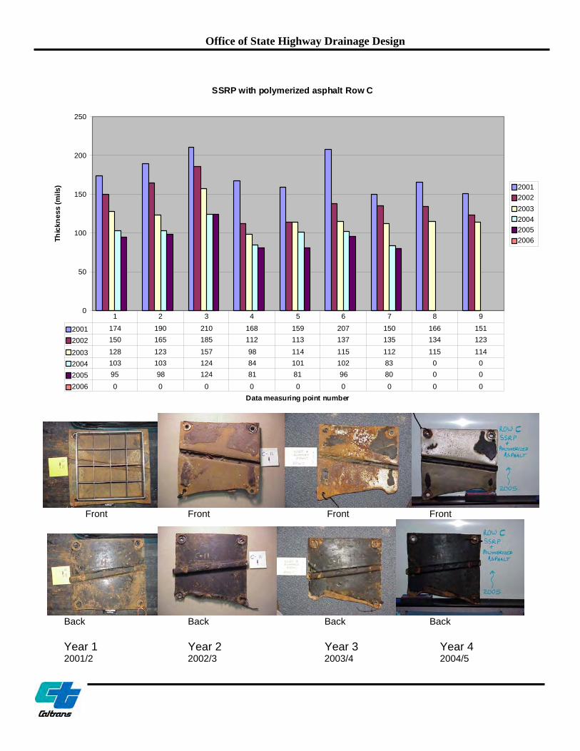
Office of State Highway Drainage Design
SSRP with polymerized asphalt Row C
0
50
100
150
200
250
Data measuring point number
Thic
knes
s (m
ils) 2001
20022003200420052006
2001 174 190 210 168 159 207 150 166 151
2002 150 165 185 112 113 137 135 134 123
2003 128 123 157 98 114 115 112 115 114
2004 103 103 124 84 101 102 83 0 0
2005 95 98 124 81 81 96 80 0 0
2006 0 0 0 0 0 0 0 0 0
1 2 3 4 5 6 7 8 9
Front Front Front Front
Back Back Back Back Year 1 Year 2 Year 3 Year 4 2001/2 2002/3 2003/4 2004/5


Office of State Highway Drainage Design
CSP with Polymeric Coating Row A
0
10
20
30
40
50
60
70
80
90
Data measuring point number
Thic
knes
s (m
ils) 2001
20022003200420052006
2001 83 84 83 82 82 83 82 83 822002 74 67 71 70 60 67 66 61 64
2003 65 62 60 56 48 70 68 51 382004 65 58 51 54 48 54 40 41 372005 57 43 49 50 48 40 33 36 31
2006 55 38 32 46 45 41 31 32 31
1 2 3 4 5 6 7 8 9
Front Front Front Front Front
Back Back Back Back Back
Year 1 Year 2 Year 3 Year 4 Year 5

Office of State Highway Drainage Design
2001/2 2002/3 2003/4 2004/5 2005/6
CSP and Polymeric Row C
0
10
20
30
40
50
60
70
80
90
100
Data measuring point number
Thic
knes
s (m
ils) 2001
20022003200420052006
2001 84 89 86 86 83 86 87 85 84
2002 69 68 72 66 67 72 64 62 73
2003 59 60 54 58 54 44 59 55 49
2004 55 54 46 55 41 32 47 53 46
2005 52 53 41 50 37 31 47 50 43
2006 44 37 22 47 37 29 45 47 35
1 2 3 4 5 6 7 8 9
Front Front Front Front Front
Back Back Back Back Back
Year 1 Year 2 Year 3 Year 4 Year 5 2001/2 2002/3 2003/4 2004/5 2005/6

Office of State Highway Drainage Design
CSP with Polymeric Coating & Polymerized Asphalt Row A
0
50
100
150
200
250
Data measuring point number
Thic
knes
s (m
ils) 2001
20022003200420052006
2001 164 177 178 202 199 193 201 212 1862002 110 114 120 139 133 129 188 159 1312003 101 89 92 122 107 107 132 117 842004 99 81 81 94 94 94 120 104 77
2005 80 74 61 86 91 92 105 81 73
2006 71 66 40 68 81 72 59 49 25
1 2 3 4 5 6 7 8 9
Front Front Front Front Front
Back Back Back Back Back
Year 1 Year 2 Year 3 Year 4 Year 5 2001/2 2002/3 2003/4 2004/5 2005/6

Office of State Highway Drainage Design
CSP with Polymeric & Polymerized Asphalt Row C
0
50
100
150
200
250
300
Data measuring point number
Thic
knes
s (m
ils) 2001
20022003200420052006
2001 234 241 186 216 229 202 206 210 200
2002 194 193 149 197 203 193 182 157 160
2003 128 115 113 142 125 115 134 121 110
2004 108 96 73 115 105 97 107 95 90
2005 102 87 61 99 98 82 99 93 72
2006 100 46 35 69 66 59 74 75 55
1 2 3 4 5 6 7 8 9
Front Front Front Front Front
Back Back Back Back Back
Year 1 Year 2 Year 3 Year 4 Year 5 2001/2 2002/3 2003/4 2004/5 2005/6

Office of State Highway Drainage Design
Aluminized CSP Row A
0
10
20
30
40
50
60
70
80
Data measuring point number
Thic
knes
s (m
ils) 2001
20022003200420052006
2001 61 60 60 61 60 59 62 62 602002 64 59 57 60 54 57 69 58 58
2003 47 47 50 49 51 50 45 49 52
2004 47 49 49 46 50 48 43 39 412005 38 46 43 38 45 42 35 30 31
2006 35 0 0 0 0 0 31 27 28
1 2 3 4 5 6 7 8 9
Front Front Front Front Front
Back Back Back Back Back
Year 1 Year 2 Year 3 Year 4 Year 5 2001/2 2002/3 2003/4 2004/5 2005/6

Office of State Highway Drainage Design
Aluminized CSP Row C
0
10
20
30
40
50
60
70
Data measuring point number
Thic
knes
s (m
ils) 2001
20022003200420052006
2001 60 61 60 59 61 60 60 60 612002 57 53 60 54 50 56 58 48 58
2003 53 45 45 43 33 34 41 35 34
2004 47 43 35 41 29 28 38 30 262005 45 40 35 38 28 25 35 30 25
2006 0 0 0 0 0 0 20 23 15
1 2 3 4 5 6 7 8 9
Front Front Front Front Front
Back Back Back Back Back
Year 1 Year 2 Year 3 Year 4 Year 5 2001/2 2002/3 2003/4 2004/5 2005/6

Office of State Highway Drainage Design
Aluminized SSRP Row B
0
10
20
30
40
50
60
70
80
Data measuring point number
Thic
knes
s (m
ils)
20012002200320042005
2001 62 61 60 61 60 59 61 60 592002 59 67 60 75 62 65 61 74 762003 51 52 50 51 57 53 54 56 56
2004 42 44 40 49 44 51 58 51 56
2005 42 33 38 44 36 39 52 50 56
1 2 3 4 5 6 7 8 9
Front Front Front Front
Year 1 Year 2 Year 3 Year 4 2001/2 2002/3 2003/4 2004/5

Office of State Highway Drainage Design
Aluminized SSRP Row D
0
10
20
30
40
50
60
70
Data measuring point number
Thic
knes
s (m
ils)
20012002200320042005
2001 62 61 62 62 65 63 60 61 64
2002 62 62 64 61 60 58 59 61 622003 61 61 62 59 63 60 62 63 61
2004 59 58 60 58 58 58 60 60 582005 53 52 58 56 56 57 54 54 54
1 2 3 4 5 6 7 8 9
Front Front Front Front
Year 1 Year 2 Year 3 Year 4 2001/2 2002/3 2003/4 2004/5

Office of State Highway Drainage Design
Galvanized CSP Row A
0
10
20
30
40
50
60
70
80
Data measuring point number
Thic
knes
s (m
ils) 2001
20022003200420052006
2001 60 60 60 60 61 60 61 60 60
2002 69 57 58 56 58 58 60 60 60
2003 52 54 53 53 57 53 53 53 53
2004 50 51 45 51 57 52 42 47 34
2005 34 37 36 44 50 43 35 34 32
2006 33 34 35 0 0 0 0 0 0
1 2 3 4 5 6 7 8 9
Front Front Front Front Front
Back Back Back Back Back
Year 1 Year 2 Year 3 Year 4 Year 5 2001/2 2002/3 2003/4 2004/5 2005/6

Office of State Highway Drainage Design
Galvanized CSP Row C
0
10
20
30
40
50
60
70
Data measuring point number
Thic
knes
s (m
ils) 2001
20022003200420052006
2001 60 58 60 60 59 60 60 60 602002 56 43 49 55 52 59 53 53 59
2003 50 45 43 53 30 43 53 47 45
2004 47 42 39 44 29 39 42 37 44
2005 38 26 27 40 20 28 39 22 24
2006 0 0 0 0 0 0 0 21 22
1 2 3 4 5 6 7 8 9
Front Front Front Front Front
Back Back Back Back Back
Year 1 Year 2 Year 3 Year 4 Year 5 2001/2 2002/3 2003/4 2004/5 2005/6

Office of State Highway Drainage Design
Galvanized SSRP Row B
0
10
20
30
40
50
60
70
80
90
Data measuring point number
Thic
knes
s (m
ils) 2001
20022003200420052006
2001 63 62 62 60 63 64 61 61 61
2002 76 55 81 61 60 64 60 51 77
2003 44 27 41 46 35 51 49 46 44
2004 43 0 40 42 29 45 47 37 43
2005 34 0 11 31 19 37 44 35 40
2006 0 0 0 0 0 0 25 0 0
1 2 3 4 5 6 7 8 9
Front Front Front Front Front
Back Back Back Back Back
Year 1 Year 2 Year 3 Year 4 Year 5 2001/2 2002/3 2003/4 2004/5 2005/6

Office of State Highway Drainage Design
Galvanized SSRP Row D
0
10
20
30
40
50
60
70
80
Data Measuring Point Number
Thic
knes
s (m
ils) 2001
20022003200420052006
2001 60 60 63 64 59 63 60 63 61
2002 64 62 64 62 66 70 62 62 642003 66 62 68 65 62 68 64 60 68
2004 55 54 62 54 57 66 62 58 652005 56 54 54 58 56 56 62 52 622006 47 51 47 47 43 54 54 42 50
1 2 3 4 5 6 7 8 9
Front Front Front Front Front
Back Back Back Back Back
Year 1 Year 2 Year 3 Year 4 Year 5 2001/2 2002/3 2003/4 2004/5 2005/6

Office of State Highway Drainage Design
0.375 inch Thick A572 Grade 50 Steel Plate Invert (Installed 2001)
0.375 inch Thick A572 Grade 50 Steel Plate Invert Measurement Reference Points (see below)
See next page for readings taken 2003, 2005 and 2006
(Study Years 2, 4, and 5)

Office of State Highway Drainage Design
2003-2006 Steel Plate Thickness (Pipe Location I)
0.29
0.31
0.33
0.35
0.37
0.39
0.41
A B C D E F G H I J K L M N O P Q R S
Location
Thic
knes
s (in
)
2003
2005
2006
2003-2006 Steel Plate Thickness (Pipe Location II)
0.29
0.31
0.33
0.35
0.37
0.39
0.41
A B C D E F G H I J K L M N O P Q R S
Location
Thic
knes
s (in
.)
200320052065
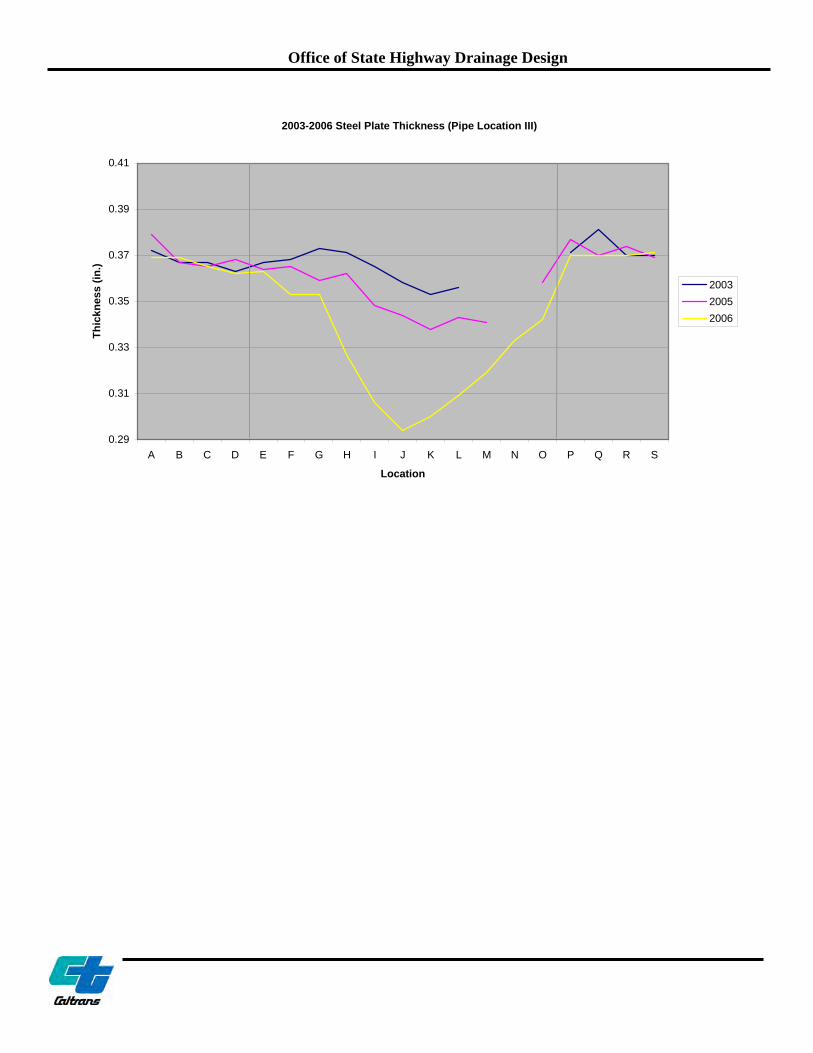
Office of State Highway Drainage Design
2003-2006 Steel Plate Thickness (Pipe Location III)
0.29
0.31
0.33
0.35
0.37
0.39
0.41
A B C D E F G H I J K L M N O P Q R S
Location
Thic
knes
s (in
.)
200320052006

Office of State Highway Drainage Design
Calcium Aluminate Mortar (Sewpercoat) - Row B
3.4
3.5
3.6
3.7
3.8
3.9
4
4.1
4.2
Data measuring point number
Thic
knes
s (in
)
20042005
2004 3.73 3.71 3.73 4.1 4.06 3.88 4.14 4.05 42005 3.73 3.7 3.73 4.08 4.03 3.86 4.02 3.93 3.97
1 2 3 4 5 6 7 8 9
Front Year 4 2004/5

APPENDIX D
References
1. A preliminary study of Aluminum as a culvert material (State of California Division of Highways, R.F. Stratfull 1964)
2. Metal loss rates of uncoated steel and aluminum culverts in New York
(Bellair/Ewing for FHWA Research Report 115, 1985)
3. Haviland, J.E.; Bellair, P.J.; Morrell, V.D. 1967. Durability of corrugated metal culverts. Physical Res. Proj. 291, Res. Rep. 66-5. Albany, NY: New York State Department of Transportation, Bureau of Physical Research
4. Abrasion resistance of polyethylene and other pipes (CSU Sacramento,
1989)
5. Field performance evaluation of polymer coated CSP structures in New York (NCSPA 2002)
6. Invert abrasion testing of CSP coatings (NCSPA 2002)
7. Field performance evaluation of uncoated CSP structures in California
(State of California, Division of Design, Office of State Highway Drainage Design, 2006) – see next page
8. Abrasion Resistance of Aluminum Culvert Based on Long-Term Field
Performance (Transportation Research Record 1087, Koepf and Ryan)
9. ADS Technical Note 2.116 Abrasion Resistance of Piping Systems, November 1, 1994 by J.B. Goddard

APPENDIX D
Field performance evaluation of uncoated CSP structures in California (State of California, Division of Design, Office of State Highway Drainage Design, 2006/7)7 Location Dia. Velocity (Q5) Bedload- Wear Rate (mils/year) (Co. Rte. PM) Description Tri-299-68.2 144” 15-20 fps Moderate (24”) 3.7- 4.3 Tri-299-70.8 144” 15-20 fps Moderate (24”) 3.7- 4.3 Tri-299-70.9 120” 15-20 fps Moderate (24”) 4.3 Sha-5-40 5-48” 7-11 fps Mod. Gravel/Stones<1” 0.5 - 3.6 Sis-96-0.6 24” 8 fps Light 2-3” 0 Sis-96-0.8 24” 6 fps Light, angular 2-3” 0 Sis-96-10.4 48” 10 fps Moderate (12”) 0 Hum-299-21.3 180” 30-40 fps Moderate (6-12”) 15 - 20 Hum-299-34.4 96” 14 fps Heavy (12”) 3-4 Nev-80-4.0 144” 17-19 fps Light (6-12”) 4.8 - 6.7 Nev-80-4.5 132” 16-17 fps Light (6-12”) 4.2 Nev-80-4.9 108” 30 fps Light (6-12”) 9 Tuo-120-24.7 96” 13-15 fps Moderate (24”) 4.6 - 6.9 Mon-1-24.1 60” 13 fps Moderate (<6”) 2-3 Mon-1-24.8 60” 22 fps Moderate (<6”) 8 Mon-1-24.9 36” 13-15 fps Moderate (<6”) 5.5 - 9.2 Mon-1-25.1 54” 19 fps Moderate (<6”) 6 - 9.2 Riv-79-31.5 24” 9-10 fps Light/Mod Sand <1 Riv-79-31.5 60” 9-10 fps Light/Mod Sand <1 Riv-215-63.4 72” 21-22 fps Coarse Sand 7-8 Sbd-18-var 5-24” 7-10 fps Lt./Well graded (2-6”) <1 SD-5-62.5 150” 21 fps Moderate/Sand 6 Lak-20-40.5 108” 13 fps Moderate/Heavy > 12” 1.2 Lak-20-40.5 108” 20 fps Moderate/Heavy > 12” 10 Lak-20-40.97 137”x 87” Arch 15.5 fps Moderate/Heavy > 12” 1 Lak-20-41.1 102” 23 fps Moderate/Heavy > 12” 10-13 Lak-20-41.17 102” 18.5 fps Moderate/Heavy > 12” 3-4 Lak-20-41.25 114”x 77” Arch 13 fps Moderate/Heavy > 12” 2 Ref. 7. See reference list previous page.

APPENDIX E
ABRASION LEVELS AND MATERIALS TABLE
Abrasion Level General Site Characteristics Invert/Pipe Materials
Level 1
• Virtually no bed load with velocities less than 5 ft/s*
* Where there are increased velocities with no bed load (e.g. urban storm drain systems or culverts < 30” dia.), significantly higher velocities may be applicable to level 1
All pipe materials listed in HDM Table 853.1A allowable for this level.No abrasive resistant protective coatings listed in HDM Table 854.3A needed for metal pipe.
Level 2
• Bed loads of sand, silts, or clays regardless of volume
• Velocities > 3 ft/s and < 8 ft/s*
* Where there are increased velocities with minor bed load volumes (e.g. urban storm drain systems or culverts < 30” dia.), significantly higher velocities may be applicable to level 2
All allowable pipe materials listed in HDM Table 853.1A with the following considerations: Generally, no abrasive resistant protective coatings needed for steel pipe. Polymeric, polymerized asphalt or bituminous coating or an additional gauge thickness of metal pipe may be specified if existing pipes in the same vicinity have demonstrated susceptibility to abrasion and thickness for structural requirements is inadequate for abrasion potential.
Level 3
• Moderate bed load volumes of sands and gravels (1.5” max).
• Velocities > 5 ft/s and < 8 ft/s*
* Where there are increased velocities with minor bed load volumes < 1.5” (e.g. storm drain systems or culverts < 30” dia.), higher velocities may be applicable to level 3
All allowable pipe materials listed in HDM Table 853.1A with the following considerations: Steel pipe may need one of the abrasive resistant protective coatings listed in HDM Table 854.3A or additional gauge thickness if existing pipes in the same vicinity have demonstrated susceptibility to abrasion and thickness for structural requirements is inadequate for abrasion potential. Aluminum pipe may require additional gauge thickness for abrasion or concrete invert protection if thickness for structural requirements is inadequate for abrasion potential. Aluminized steel (type 2) not recommended without invert protection or increased gauge thickness (equivalent to galv. Steel) where pH < 6.5 and resistivity < 20,000. Lining alternatives: PVC, Corrugated or Solid Wall HDPE, CIPP (with min. thickness for abrasion specified)
Level 4
• Small to moderate bed load volumes of sands, gravels, and/or small cobbles/rocks with maximum stone sizes up to about 6 in.
• Velocities > 8 ft/s and < 12 ft/s
All allowable pipe materials listed in HDM Table 853.1A with the following considerations: Steel pipe will typically need one of the abrasive resistant protective coatings listed in HDM Table 854.3A or may need additional gauge thickness if thickness for structural requirements is inadequate for abrasion potential. Aluminum may require additional gauge thickness or concrete invert protection if thickness for structural requirements is inadequate for abrasion potential. Aluminized steel (type 2) not recommended without invert protection or increased gauge thickness (wear rate equivalent to galv. steel) where pH < 6.5 and resistivity < 20,000 if thickness for structural requirements is inadequate for abrasion potential. Increase concrete cover over reinforcing steel for RCB (invert only). RCP generally not recommended. Lining alternatives: Closed profile or SDR 35 PVC (corrugated and ribbed PVC limited to 36” min. diameter. Machine-wound PVC not recommended. SDR HDPE (corrugated HDPE Type S limited to 48” min. diameter, corrugated HDPE Type C not recommended). CIPP (min. thickness for abrasion specified), concrete.
Level 5
• See next page
Aluminum may require additional gauge thickness or concrete invert protection if thickness for structural requirements is inadequate for abrasion potential (see lining alternatives below). Aluminized steel (type 2) not recommended without invert protection or increased gauge thickness (wear rate equivalent to galv. steel) where pH < 6.5 and resistivity < 20,000 if thickness for structural requirements is inadequate for abrasion potential. Closed profile and SDR 35 PVC liners allowed but not recommended

APPENDIX E
Level 5
• Moderate bed load volumes of sands, gravels, and/or small cobbles with maximum stone sizes up to about 6 in. For larger stone sizes within this velocity range, see Level 6
• Velocities > 12 ft/s and < 15 ft/s
for upper range of stone sizes in bed load if freezing conditions are often encountered, otherwise OK for stone sizes up to 3 in. Most abrasive resistant coatings listed in HDM Table 854.3A are not recommended for steel pipe. A concrete invert lining or additional gauge thickness is recommended if thickness for structural requirements is inadequate for abrasion potential. See lining alternatives below. Increase concrete cover over reinforcing steel for RCB (invert only). RCP generally not recommended Lining alternatives: Closed profile (>30 in) or SDR 35 PVC (corrugated and ribbed not recommended. Machine-wound PVC not recommended), SDR HDPE (corrugated Type S and Type C not recommended), RPMP, CIPP (with min. thickness for abrasion specified), concrete.
Level 6
• Heavy bed load volumes of sands, gravel and rocks, with stone sizes 6 in or larger
• Velocities > 12 ft/s and < 20 ft/s
or
• Heavy bed load volumes of sands, gravel and small cobbles, with stone sizes up to about 6 in
• Velocities > 15 ft/s and < 20 ft/s*
*Very limited data on abrasion resistance for velocities > 20 ft/s; contact District Hydraulics Branch.
Aluminum pipe requires additional gauge thickness and concrete invert protection (see lining alternatives below). Aluminized steel (type 2) not recommended without invert protection or increased gauge thickness (wear rate equivalent to galv. steel) where pH < 6.5 and resistivity < 20,000. None of the abrasive resistant protective coatings listed in HDM Table 854.3A are recommended for protecting steel pipe. A concrete invert lining and additional gauge thickness is recommended. See lining alternatives below. Corrugated HDPE not recommended. Corrugated and closed profile PVC pipe not recommended. RCP not recommended. Increase concrete cover over reinforcing steel recommended for RCB (invert only) for velocities up to 15 ft/s. RCB not recommended for bed load stone sizes > 3 in and velocities greater than 15 ft/s unless concrete lining with larger, harder aggregate is placed (see lining alternatives below). SDR 35 PVC liners (> 36 in) allowed but not recommended for upper range of stone sizes in bed load if freezing conditions are often encountered, otherwise OK for stone sizes up to 3 in. Lining/replacement alternatives: SDR 35 PVC (see note above) or HDPE SDR (minimum wall thickness 1”), CIPP (with min. thickness for abrasion specified), class 2 concrete with embedded aggregate (e.g. cobbles or RSP (facing)): (for all bed load sizes a larger, harder aggregate than the bed load, decreased water cement ratio and an increased concrete compressive strength should be specified). Alternative invert linings may include steel plate, rails or concreted RSP, and abrasion resistant concrete (Calcium Aluminate). For new/replacement construction, consider “bottomless” structures.

APPENDIX E
Anticipated Service Life Added to Steel Pipe (in Years) by Abrasive
Resistant Protective Coating
Flow Vel. (ft/s)
Channel Materials
Bituminous Coating
(yrs.)(hot-dipped)
Bituminous Coating &
Paved Invert (yrs.)
Polymerized Asph.
(yrs.)(hot-dipped)
Polymeric Sheet
Coating. (yrs.)
Polyethylene (CSSRP)
<5 See note 1
Non-Abrasive
8 15 * * *
>3 - <8
See note 2
Abrasive
6-0
15-2
30-5
30-5
*
>8 - <12
Abrasive
0
2-0
5-0
5-0
70-35
>12-<15
Abrasive
** ** ** ** 35-8***
>15-<20 or
>12-<20
Abrasive &
heavy bedloads
**** **** **** **** ****
* Provides adequate abrasion resistance to meet or exceed a 50-year design service life. ** Abrasive resistant protective coatings not recommended, increase steel thickness to 10 gage *** Not recommended above 14 fps flow velocity ****Contact District Hydraulics Branch. Note 1. Where there are increased velocities with no bedload (e.g. urban storm drain systems or culverts < 30” dia.), higher velocities may be applicable
Note 2. Where there are increased velocities with minor bedload (e.g. urban storm drain systems or culverts < 30” dia.), higher velocities may be applicable Note 3. Range of additional service life commensurate with flow velocity range

APPENDIX E
Anticipated additional wear (in mils/year) to steel pipe for abrasion levels 4 through 6
0.5
1
3.5
2.5
10
0
1
2
3
4
5
6
7
8
9
10
8 9 10 11 12 13 14 15 16 17 18 19 20
Velocity (fps)
Wea
r (m
ils/y
ear)
Legend Blue: Abrasion levels 4 and 5 Pink: Abrasion level 6
Note: No additional wear for abrasion levels 1 through 3. See HDM Figure 854.3C for estimating years to perforation.

APPENDIX F
Jones Bar (S Fk Yuba River) and Shady Creek Gage Comparison (1/1-3/31 2004)
0
500
1000
1500
2000
2500
3000
3500
Month
Peak
sto
rm fl
ow (c
fs)
Jones Bar
Shady Creek
Jones Bar 373 194 508 686 328 2834 2953 700 3104 855 561
Shady Creek 37 16 92 56 32 133 252 25 303 49 16
Jan Jan Jan Feb Feb Feb Feb Feb Feb Mar Mar
Rainfall 0.6” 0.37” 1.65” 1.3” 0.4” 1.2” 1.6” 0.3” 1.5” 0.75” 0.6” Bedload Tons/Day
18 1.5 150 40 15 180 700 8 1050 40 1.5
Jones Bar (Middle Fork,Yuba River) peak flow event summary during five year abrasion study at Shady Creek

APPENDIX F
Jones Bar Gage Volume Flow Rate (2001-2006)
0
5000
10000
15000
20000
25000
30000
Oct
Dec Jan
Mar
Nov
Dec
Feb
Apr
Apr
Aug
Dec
Dec
Feb
Mar
Nov Jan
Feb
Mar
May Oct
Dec Jan
Feb
Mar
Apr
May
Date
Peak
sto
rm fl
ow (c
fs)
2001-2002 2002-2003 2003-2004 2004-2005 2005-2006
Jones Bar (Middle Fork,Yuba River) peak flow event summary during five year abrasion study at Shady Creek