Qian et al. EURASIP Journal onWireless Communications andNetworking (2016) 2016:148 DOI 10.1186/s13638-016-0650-0

RESEARCH Open Access

Energy-efficient data disseminationstrategy for roadside infrastructure in VCPSJin Qian*, Tao Jing, Yan Huo, Hui Li and Zhen Li

Abstract

In vehicular cyber-physical system (VCPS), beaconing mechanism is commonly deployed for the solar-poweredroadside infrastructure to detect available passing-by vehicles for data dissemination. The traditional beaconingmechanism would cause a higher energy consumption due to the periodical beaconing procedure. To tackle thisproblem, we propose a new data dissemination strategy for roadside infrastructures by adjusting the beaconinginterval to reduce the energy consumption. We model the beaconing procedure as a Markov model by observing theperiodical beaconing results and then using the modeling result to obtain the relationship between the beaconinginterval and the expectation of the single-vehicle discovery time. Then, with the average data transmission raterequirement, we can calculate the maximum beaconing interval. We also introduce a satisfaction degree based onthe Sigmoid function to combine the decreased energy consumption and the decreased data rate. The satisfactiondegree function allows the roadside infrastructure to obtain the optimal beaconing interval based on the requiredquality of service. The analysis of the results show that careful tuning of key parameters leads to improved energyefficiency and increased data rate of the data dissemination strategy.

Keywords: VCPS, Beaconing interval, Markov model

1 IntroductionCyber-physical system (CPS) is a complex system withintricate interplay between the physical world andthe cyber world [1–4]. Vehicular cyber-physical system(VCPS) is a typical CPS applied in the intelligent trans-portation field. It has attracted a significant amount ofinterests in the past few decades [5–8]. VCPS holds greatpotential in enhancing vehicle safety and improving traf-fic efficiency. It also can make a further contribution topassengers’ comfort by providing infotainment services.In VCPS, roadside infrastructures play an important

role. They are usually deployed in highways or road inter-sections and can communicate with passing-by vehiclesthrough dedicated short-range communications (DSRC)technologies. According to the difference of the structureand the function, roadside infrastructures could generallybe divided into two types. One is with a large commu-nication coverage and high processing capability [9–11].They are used as wireless gateway nodes that interconnect

*Correspondence: qianjin@bjtu.edu.cnSchool of Electronics and Information Engineering, Beijing Jiaotong University,Haidian, 100044 Beijing, China

vehicular ad hoc networks and a wired network (i.e., theInternet), providing Internet connectivity to the vehicles.Also, they offer the real-time traffic status to the vehicles.The other kind is the simple structure roadside infras-tructure just with the capability to disseminate data [12].It disseminates the data stored in the infrastructure tothe passing-by vehicles periodically. Generally, these dataare the advertising messages. Due to the characteristics ofthe convenient installation and the relatively low cost ofthese simple structure roadside infrastructures, they havebeen widely used in VCPS.With the massive uses of them,the information content diversity of the whole networkwill be enriched leading to a further improvement of theVCPS. The research objects of this paper are these simplestructure roadside infrastructures.These simple structure roadside infrastructures are

massively deployed in locations like the highway. Nor-mally, they use the solar as power input due to theunavailability or excess expense of wired electrical power.While the provisioning cost of a solar-powered roadsideinfrastructure is a strong function of its average energyconsumption. According to the analysis in [13] which is

© 2016 Qian et al. Open Access This article is distributed under the terms of the Creative Commons Attribution 4.0 InternationalLicense (http://creativecommons.org/licenses/by/4.0/), which permits unrestricted use, distribution, and reproduction in anymedium, provided you give appropriate credit to the original author(s) and the source, provide a link to the Creative Commonslicense, and indicate if changes were made.

Qian et al. EURASIP Journal onWireless Communications and Networking (2016) 2016:148 Page 2 of 13

a part of the US Department of Transportation’s Vehi-cle Infrastructure Integration Initiative, a breakdown ofthe deployment costs also found that over 63% of theseroadside infrastructure costs would be consumed by solarenergy provisioning, e.g., solar panels, batteries, and theirassociated electronics. So, it is important to reduce theenergy consumption of the simple structure roadsideinfrastructures.The energy consumption is mainly composed of two

parts: the energy consumed in the wireless commu-nication and the energy consumed in the informationprocessing and computing. The radio is the most energy-consuming component, taking nearly 30 times the energyof the microcontroller unit used in the simple struc-ture roadside infrastructures [14]. Therefore, to reducethe energy consumption, the key point is to improve theenergy efficiency of the wireless communication.For these simple structure roadside infrastructures, the

basic mechanism of the traditional data disseminationstrategy is beaconing [15, 16]. Beacon packets are period-ically and locally broadcasted by a roadside infrastructureto announce its current status and detect whether thereare suitable vehicles to disseminate the data to. One vehi-cle in the communication range that successfully receivesthe beacon packet needs to reply an acknowledgment(ACK) packet. After receiving the ACK packet, the road-side infrastructure can get the status of the vehicle. Then,it can decide whether to start the data transmission pro-cess or not based on the status of the vehicle and thespecific data content. In our research, we find that if thevehicle density is relatively low around the location wherethe roadside infrastructure is deployed, due to the limitednumber of the passing-by vehicles, just a few numbers ofthe beacon packets get a reply. Most of the beacon packetsare ineffective. Although the beacon packet is small, largernumbers of ineffective beacon packets cause a high energywaste.In this paper, we design an energy-efficient data dissem-

ination strategy for roadside infrastructures by adjustingthe beaconing interval. We design two phases for thenew data dissemination strategy. The first is the model-ing phase. The second is the applying phase. We modelthe beaconing procedure as a Markov model by observ-ing the periodical beaconing results in the modeling phaseand then use the modeling result in choosing a new bea-coning interval in the applying phase. With the averagedata transmission rate requirement, we can calculate themaximum beaconing interval. By using the Sigmoid func-tion, we can obtain the optimal beaconing interval basedon the satisfaction degree. Through the proposed strategy,we can increase the effectiveness of the beaconing packetsand improve the energy efficiency of the data dissemina-tion strategy. Our main contributions are summarized asfollows:

1. According to the Markov property of the presence ofthe passing-by vehicles, we present the statetransition probabilities for the Markov model of thebeaconing results by using the maximum likelihoodmethod. Meanwhile, we calculate the duration of themodeling phase within which the modeling canguarantee a certain accuracy based on the centrallimit theorem.

2. We obtain the relationship between the beaconinginterval and the expectation of the single-vehiclediscovery time based on the state transitionprobabilities. The single-vehicle discovery timemeans the time interval between the adjacent twotimes when the roadside infrastructure discovery onevehicle. With the average data transmission raterequirement which is related to the single-vehiclediscovery time, we can calculate the maximumbeaconing interval.

3. We introduce a satisfaction degree based on theSigmoid function to combine the decreased energyconsumption and the decreased data rate effectively.If we want to choose a smaller beaconing intervalthan the maximum beaconing interval and obtain ashorter single-vehicle discovery time, we can use thesatisfaction degree function to obtain the optimalbeaconing interval which can balance the tradeoffbetween energy consumption and the average datatransmission rate.

4. We demonstrate that the proposed datadissemination strategy can significantly reduce theenergy consumption while satisfying the servicequality requirement. The impact of the systemparameters on the data dissemination strategy isinvestigated via extensive simulation study. Theanalysis of the results show that careful tuning of keyparameters leads to improved energy efficiency andincreased data rate of the data dissemination strategy.

The rest of the paper is organized as follows. Relatedwork is outlined in Section 2. Our system model andthe problem definition are described in Section 3. InSection 4, we describe the detail of the modeling phase.The applying phase is described in Section 5. Thewhole beaconing interval optimization process is given inSection 6. In Section 7, we make a numerical analysis ofour strategy. The conclusion is finalized in Section 8.

2 Related workFor the roadside infrastructures, energy conservationin the data dissemination strategy guarantees the effi-cient usage of energy, which makes great contributionto the commercial application of VCPS. Recently, manyresearches have been made to improve energy efficiency.In [17], by using a mixed-integer linear programming

Qian et al. EURASIP Journal onWireless Communications and Networking (2016) 2016:148 Page 3 of 13

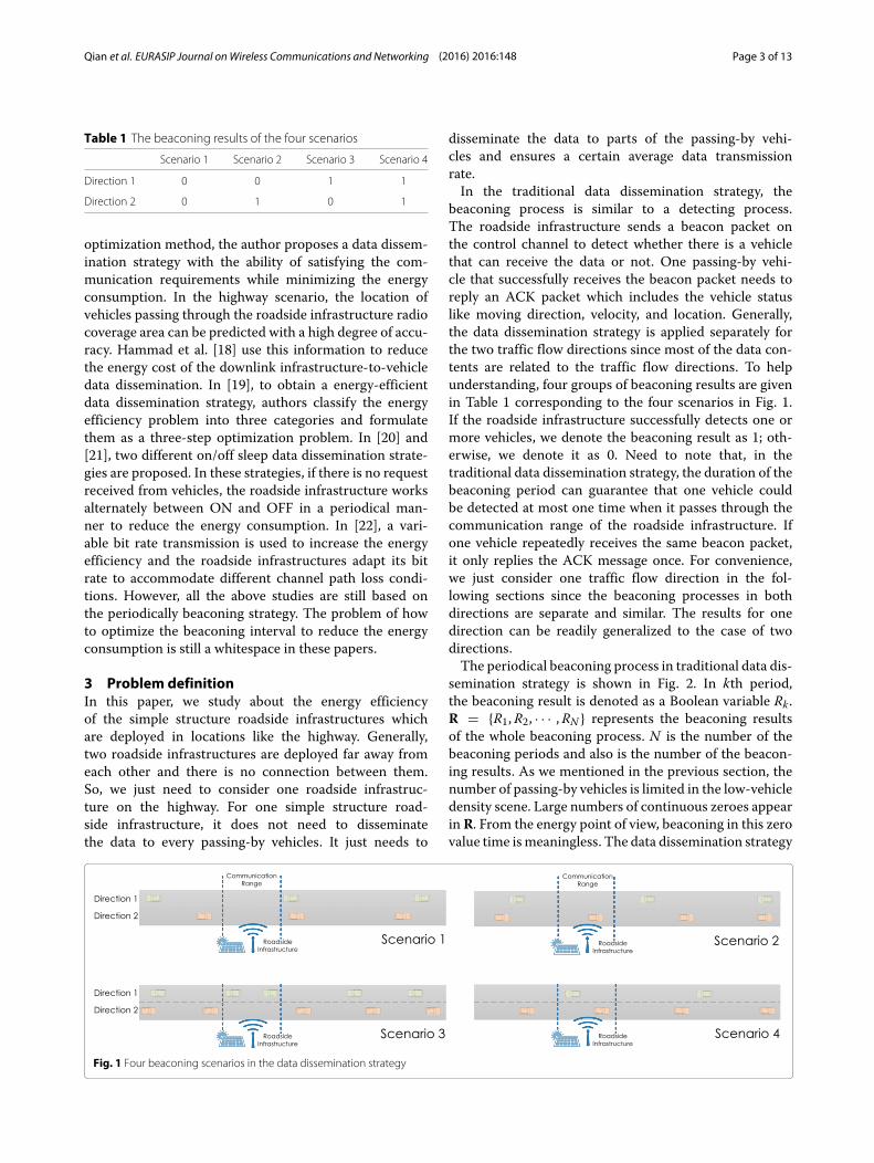
Table 1 The beaconing results of the four scenarios

Scenario 1 Scenario 2 Scenario 3 Scenario 4

Direction 1 0 0 1 1

Direction 2 0 1 0 1

optimization method, the author proposes a data dissem-ination strategy with the ability of satisfying the com-munication requirements while minimizing the energyconsumption. In the highway scenario, the location ofvehicles passing through the roadside infrastructure radiocoverage area can be predicted with a high degree of accu-racy. Hammad et al. [18] use this information to reducethe energy cost of the downlink infrastructure-to-vehicledata dissemination. In [19], to obtain a energy-efficientdata dissemination strategy, authors classify the energyefficiency problem into three categories and formulatethem as a three-step optimization problem. In [20] and[21], two different on/off sleep data dissemination strate-gies are proposed. In these strategies, if there is no requestreceived from vehicles, the roadside infrastructure worksalternately between ON and OFF in a periodical man-ner to reduce the energy consumption. In [22], a vari-able bit rate transmission is used to increase the energyefficiency and the roadside infrastructures adapt its bitrate to accommodate different channel path loss condi-tions. However, all the above studies are still based onthe periodically beaconing strategy. The problem of howto optimize the beaconing interval to reduce the energyconsumption is still a whitespace in these papers.

3 Problem definitionIn this paper, we study about the energy efficiencyof the simple structure roadside infrastructures whichare deployed in locations like the highway. Generally,two roadside infrastructures are deployed far away fromeach other and there is no connection between them.So, we just need to consider one roadside infrastruc-ture on the highway. For one simple structure road-side infrastructure, it does not need to disseminatethe data to every passing-by vehicles. It just needs to

disseminate the data to parts of the passing-by vehi-cles and ensures a certain average data transmissionrate.In the traditional data dissemination strategy, the

beaconing process is similar to a detecting process.The roadside infrastructure sends a beacon packet onthe control channel to detect whether there is a vehiclethat can receive the data or not. One passing-by vehi-cle that successfully receives the beacon packet needs toreply an ACK packet which includes the vehicle statuslike moving direction, velocity, and location. Generally,the data dissemination strategy is applied separately forthe two traffic flow directions since most of the data con-tents are related to the traffic flow directions. To helpunderstanding, four groups of beaconing results are givenin Table 1 corresponding to the four scenarios in Fig. 1.If the roadside infrastructure successfully detects one ormore vehicles, we denote the beaconing result as 1; oth-erwise, we denote it as 0. Need to note that, in thetraditional data dissemination strategy, the duration of thebeaconing period can guarantee that one vehicle couldbe detected at most one time when it passes through thecommunication range of the roadside infrastructure. Ifone vehicle repeatedly receives the same beacon packet,it only replies the ACK message once. For convenience,we just consider one traffic flow direction in the fol-lowing sections since the beaconing processes in bothdirections are separate and similar. The results for onedirection can be readily generalized to the case of twodirections.The periodical beaconing process in traditional data dis-

semination strategy is shown in Fig. 2. In kth period,the beaconing result is denoted as a Boolean variable Rk .R = {R1,R2, · · · ,RN } represents the beaconing resultsof the whole beaconing process. N is the number of thebeaconing periods and also is the number of the beacon-ing results. As we mentioned in the previous section, thenumber of passing-by vehicles is limited in the low-vehicledensity scene. Large numbers of continuous zeroes appearin R. From the energy point of view, beaconing in this zerovalue time ismeaningless. The data dissemination strategy

Fig. 1 Four beaconing scenarios in the data dissemination strategy

Qian et al. EURASIP Journal onWireless Communications and Networking (2016) 2016:148 Page 4 of 13

Fig. 2 The periodical beaconing process in the traditional data dissemination strategy

will be more energy efficient if the roadside infrastruc-ture broadcasts the beacon packets with a certain inter-val instead of broadcasting them in each period. This isthe core idea of our proposed strategy. Intuitively, if thebeaconing interval is too long, the roadside infrastruc-ture may miss too many dissemination opportunities. Ifthe beaconing interval is too short, there is no obviousimprovement in the energy efficiency. How to obtain asuitable beaconing interval is the most important problemin our study. As shown in Fig. 3, we design a model-ing phase and an applying phase in our energy-efficientdata dissemination strategy. In the modeling phase, likethe traditional data dissemination strategy, the roadsideinfrastructure sends the beacon packets periodically tolearn the presence of passing-by vehicles. The duration ofone period defined as t0. t0 is very small. In the applyingphase, the roadside infrastructure calculates the optimalbeaconing intervals defined as ta and tb. If the initial bea-coning result is 0, the roadside infrastructure sends thebeacon packets with time interval ta, otherwise with tb.The detail of the new strategy is shown in the followingsections.

4 Themodeling phaseNormally, the research objects of our paper are deployedon the highway. The existence of the Markov propertyin the scenario of highway has been validated in[23–25]. Since the beaconing results are directly relatedto the presences of the passing-by vehicles, we can modelthe traditional beaconing procedure as a continuous-timeMarkov process. We define the state space as X = {x1, x2},

with x1 = 0 and x2 = 1 indicating that the beaconingresults are 0 and 1. The state transition probability matrix

is defined as P(t) =(P00(t) P01(t)P10(t) P11(t)

), where Pij(t) =

P(Rs+t = j|Rs = i), i, j ∈ {0, 1}.

4.1 The state transition probabilities when the beaconingperiod is t0

As shown in Fig. 3, we define M as the number of thebeaconing periods in the modeling phase. We define R ={R1,R2, · · · ,RM} with Rm ∈ X for ∀m ∈ {1, · · · ,M} asthe beaconing results. After theM beaconing periods, theroadside infrastructure can get the beaconing result sam-ples denoted as r1, r2, · · · , rM. Based on these samples,we can estimate the state transition probabilities of theMarkov model. The state transition probability matrix is

denoted as P(t0) =(P00(t0) P01(t0)P10(t0) P11(t0)

), where Pij(t0) =

P(Rs+t0 = j|Rs = i), i, j ∈ {0, 1}, s = {1t0, 2t0, · · · , (M −1)t0}. Since it can be understood that the discrete-timeMarkov chain is the discretization of the continuous-timeMarkov chain, when the time slot is very small, theyare identical in essence. According to this property, weuse the maximum likelihood estimation method that isused in the discrete-time Markov chain to estimate tran-sition probability. The maximum likelihood estimation isconsistent and asymptotically unbiased. The counts ofthe occurrence of four different transition types such as(rk , rk+1) = (0, 0), (0, 1), (1, 0), (1, 1) are defined as n00,n01, n10, and n11, k = {1, 2, · · · ,M − 1}. The likelihoodfunction is given by

Fig. 3 The beaconing process in our new energy-efficient data dissemination strategy

Qian et al. EURASIP Journal onWireless Communications and Networking (2016) 2016:148 Page 5 of 13

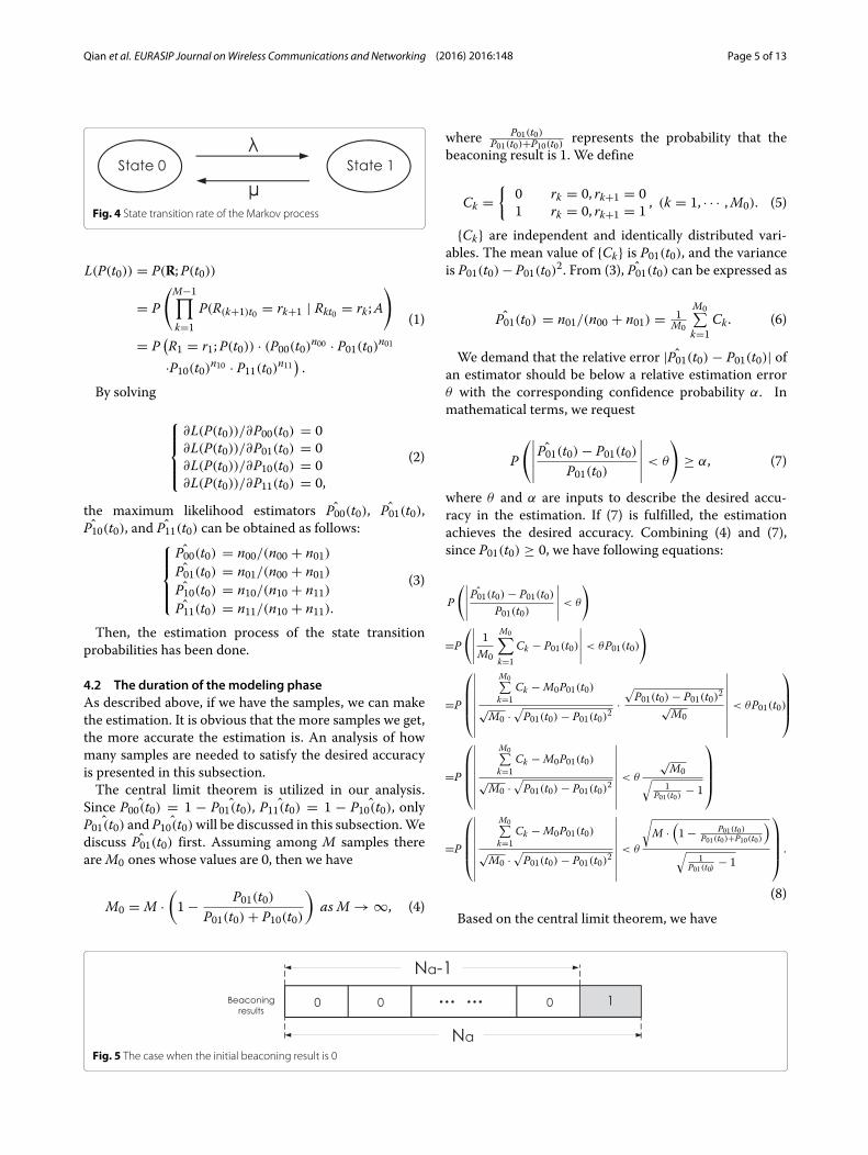
Fig. 4 State transition rate of the Markov process

L(P(t0)) = P(R;P(t0))

= P(M−1∏

k=1P(R(k+1)t0 = rk+1 | Rkt0 = rk ;A

)= P

(R1 = r1;P(t0)) · (P00(t0)n00 · P01(t0)n01·P10(t0)n10 · P11(t0)n11

).

(1)

By solving

⎧⎪⎪⎨⎪⎪⎩∂L(P(t0))/∂P00(t0) = 0∂L(P(t0))/∂P01(t0) = 0∂L(P(t0))/∂P10(t0) = 0∂L(P(t0))/∂P11(t0) = 0,

(2)

the maximum likelihood estimators ˆP00(t0), ˆP01(t0),ˆP10(t0), and ˆP11(t0) can be obtained as follows:⎧⎪⎪⎨⎪⎪⎩ˆP00(t0) = n00/(n00 + n01)ˆP01(t0) = n01/(n00 + n01)ˆP10(t0) = n10/(n10 + n11)ˆP11(t0) = n11/(n10 + n11).

(3)

Then, the estimation process of the state transitionprobabilities has been done.

4.2 The duration of the modeling phaseAs described above, if we have the samples, we can makethe estimation. It is obvious that the more samples we get,the more accurate the estimation is. An analysis of howmany samples are needed to satisfy the desired accuracyis presented in this subsection.The central limit theorem is utilized in our analysis.

Since ˆP00(t0) = 1 − ˆP01(t0), ˆP11(t0) = 1 − ˆP10(t0), onlyˆP01(t0) and ˆP10(t0)will be discussed in this subsection.Wediscuss ˆP01(t0) first. Assuming among M samples thereareM0 ones whose values are 0, then we have

M0 = M ·(1 − P01(t0)

P01(t0) + P10(t0)

)as M → ∞, (4)

where P01(t0)P01(t0)+P10(t0) represents the probability that the

beaconing result is 1. We define

Ck ={

0 rk = 0, rk+1 = 01 rk = 0, rk+1 = 1 , (k = 1, · · · ,M0). (5)

{Ck} are independent and identically distributed vari-ables. The mean value of {Ck} is P01(t0), and the varianceis P01(t0) − P01(t0)2. From (3), ˆP01(t0) can be expressed as

ˆP01(t0) = n01/(n00 + n01) = 1M0

M0∑k=1

Ck . (6)

We demand that the relative error | ˆP01(t0) − P01(t0)| ofan estimator should be below a relative estimation errorθ with the corresponding confidence probability α. Inmathematical terms, we request

P(∣∣∣∣∣ ˆP01(t0) − P01(t0)

P01(t0)

∣∣∣∣∣ < θ

)≥ α, (7)

where θ and α are inputs to describe the desired accu-racy in the estimation. If (7) is fulfilled, the estimationachieves the desired accuracy. Combining (4) and (7),since P01(t0) ≥ 0, we have following equations:

P(∣∣∣∣∣ ˆP01(t0) − P01(t0)

P01(t0)

∣∣∣∣∣ < θ

)

=P(∣∣∣∣∣ 1

M0

M0∑k=1

Ck − P01(t0)

∣∣∣∣∣ < θP01(t0))

=P

⎛⎜⎜⎜⎝∣∣∣∣∣∣∣∣∣

M0∑k=1

Ck − M0P01(t0)

√M0 ·

√P01(t0) − P01(t0)2

·√P01(t0) − P01(t0)2√

M0

∣∣∣∣∣∣∣∣∣ < θP01(t0)

⎞⎟⎟⎟⎠

=P

⎛⎜⎜⎜⎝∣∣∣∣∣∣∣∣∣

M0∑k=1

Ck − M0P01(t0)

√M0 ·

√P01(t0) − P01(t0)2

∣∣∣∣∣∣∣∣∣ < θ

√M0√1

P01(t0) − 1

⎞⎟⎟⎟⎠

=P

⎛⎜⎜⎜⎝∣∣∣∣∣∣∣∣∣

M0∑k=1

Ck − M0P01(t0)

√M0 ·

√P01(t0) − P01(t0)2

∣∣∣∣∣∣∣∣∣ < θ

√M ·

(1 − P01(t0)

P01(t0)+P10(t0)

)√

1P01(t0) − 1

⎞⎟⎟⎟⎠ .

(8)

Based on the central limit theorem, we have

Fig. 5 The case when the initial beaconing result is 0

Qian et al. EURASIP Journal onWireless Communications and Networking (2016) 2016:148 Page 6 of 13

Table 2 The relationship between ETa(ta) and ta

ETa(ta) 0.5 1.0 1.5 2.0 2.5 3.0

ta 0.28 0.59 0.91 1.23 1.49 1.82

M0∑k=1

Ck − M0P01(t0)

√M0 ·

√P01(t0) − P01(t0)2

→ N(0, 1) as M0 → ∞. (9)

We denote �(•) as the standard normal cumulativedistribution function. Then, we have

2�

⎛⎜⎜⎝θ

√M ·

(1 − P01(t0)

P01(t0)+P10(t0)

)√

1P01(t0) − 1

⎞⎟⎟⎠ − 1 ≥ α. (10)

In (10),M > 0, 0 ≤ P01(t0) ≤ 1 and 0 ≤ P10(t0) ≤ 1.WedenoteMa

min as theminimum required number of the bea-coning result samples for ˆP01(t0). For any state transitionprobability values,Ma can be expressed as follows:

Mamin =

(�−1( 1+α

2 ))2

θ2(1 − P01(t0))

(1

P01(t0)+ 1

P10(t0)

). (11)

For ˆP10(t0), the analysis process is the same. The mini-mum required number of the beaconing result samples forˆP01(t0) is denoted asMb

min. We have

Mbmin =

(�−1 ( 1+α

2))2

θ2(1 − P10(t0))

(1

P01(t0)+ 1

P10(t0)

). (12)

Therefore, when the desired accuracy α and θ are given,we have the following equations:

Mmin = max{Ma

min,Mbmin

}, (13)

whereMmin is denoted as the minimum required numberof the beaconing result samples for the estimation.Actually, since we do not know the values of P01(t0)

and P10(t0) before we start the modeling phase, we cannotcalculate the required number of the samples. To tacklethis problem, we have the following processes. At the

beginning of the modeling phase, we send Mdefault bea-con packets firstly. The value ofMdefault is analyzed in thelater section. According to the Mdefault beaconing resultsamples, we can calculate the P01(t0) and P10(t0). Then,we can get the Mmin. If Mmin ≤ Mdefault, it means theestimation of the state transition probabilities reaches thedesired accuracy, and we can stop the modeling phase.If not, the periodical beaconing continues. We denoteMactual as the actual number of the beacon packets. Aftereach of the continuous beaconing processes, we recal-culate the Mmin and compare it with the Mactual. UntilMactual ≥ Mmin, we stop the periodical beaconing andstart the applying phase. The total beaconing times of themodeling phaseMtotal is equal to the currentMactual. Thetotal duration of the modeling phase is expressed as

Tmodeling = t0Mtotal. (14)

Through the above analyses, we can summarize thefollowing proposition:

Proposition 1. After acquiring a certain number of sam-ples, the estimation of the state transition probabilities forthe Markov process can achieve a desired accuracy.

5 The applying phaseAfter obtaining the state transition probabilities when thebeaconing period is t0, we can calculate the system param-eters of the Markov process. Then, we can obtain theoptimal beaconing interval and apply it in the applyingphase.

5.1 The state transition probabilities in the applyingphase

We define the state transition rate matrix of the Markovprocess as

Q =(−λ λ

μ −μ

), (15)

where λ and μ are the arrival rate and the departure rateshown in Fig. 4. The state transition probabilities can bederived from the matrix Q. We have

Fig. 6 The case when the initial beaconing result is 1

Qian et al. EURASIP Journal onWireless Communications and Networking (2016) 2016:148 Page 7 of 13

Table 3 The relationship between ETa(tb), ta , and tb

ETb(tb) 0.5 1.0 1.5 2.0 2.5 3.0

ta 0.28 0.59 0.91 1.23 1.49 1.82

tb 0.23 0.49 0.78 1.11 1.30 1.57

⎧⎪⎪⎪⎨⎪⎪⎪⎩P00(t) = μ

λ+μ+ λ

λ+μe−(λ+μ)t

P01(t) = λλ+μ

− λλ+μ

e−(λ+μ)t

P10(t) = μλ+μ

− μλ+μ

e−(λ+μ)t

P11(t) = λλ+μ

+ μλ+μ

e−(λ+μ)t

. (16)

In the modeling phase, we have obtained the estimationresults ˆP00(t0), ˆP01(t0), ˆP10(t0), and ˆP11(t0). Combiningwith the beaconing period t0, we obtain

⎧⎪⎪⎪⎪⎨⎪⎪⎪⎪⎩λ =

( ˆP01(t0))log

(1

1− ˆP01(t0)− ˆP10(t0)

)( ˆP01(t0)+ ˆP10(t0)

)t0

μ =( ˆP10(t0)

)log

(1

1− ˆP01(t0)− ˆP10(t0)

)( ˆP01(t0)+ ˆP10(t0))t0

. (17)

According to (16) and (17), we can calculate the statetransition probabilities in any value of t.

5.2 The optimal beaconing interval when the initialbeaconing result is 0

Figure 5 illustrates the case when the initial beaconingresult is 0. We denoteNa as the beaconing times such thatthe roadside infrastructure can discover one passing-byvehicle in this case. Obviously, the first Na − 1 beacon-ing results are 0, the final one is 1. The probability massfunction of Na can be represented as

P(Na = n) ={P01(ta)Pn−1

00 (ta) n ≥ 10 others . (18)

Table 4 Simulation parametersParameter Value

The length of a beaconing period t0 0.1 s

The confidence probability value α 99%

Relative estimation error θ 20%

Energy used for each beaconing ξ 10mJ

Average amount of data in each transmission process ω 300 kbit

Threshold δaE 90

Threshold δaR 5.5

Threshold δbE 16

Threshold δbR 600

The expectation of the required beaconing timesENa(ta) is

ENa(ta) =∞∑n=1

nP01(ta)Pn−100 (ta)

= P01(ta)1 + P200(ta) − 2P00(ta)

.(19)

Therefore, the expectation of single-vehicle discoverytime ETa(ta) is

ETa(ta) = ta · ENa(ta). (20)

When ˆP01(t0) = 0.28 and ˆP10(t0) = 0.40, we haveTable 2.All the calculated beaconing intervals are larger than

t0 = 0.1. The energy consumption decreases.

5.2.1 Themaximumbeaconing intervalWe denote the average data transmission rate require-ment as D. The average amount of data in each of datatransmission process is denoted as ω. Then, we have

D ≤ ω

ETa(ta). (21)

According to (18), (19), and (20), we can calculate themaximum ta which is denoted as tmax

a .

5.2.2 The optimal beaconing intervalGenerally, in the real system, we do not always need touse the maximum beaconing interval. Under the con-dition that there is an average data transmission raterequirement, we need to calculate an optimal beacon-ing interval that can balance the tradeoff between energyconsumption and the average data transmission rate. Inthis paper, we introduce a satisfaction degree based onthe Sigmoid function to combine the decreased energy

Fig. 7 The relationship between the required number of samples andthe state transition probabilities

Qian et al. EURASIP Journal onWireless Communications and Networking (2016) 2016:148 Page 8 of 13

consumption and the decreased data rate effectively. TheSigmoid function has been widely employed to approx-imate users’ satisfaction with respect to service qualityor resource allocation. The optimal beaconing intervalcalculation process is shown as follows.When the initial beaconing result is 0, the average

decreased energy consumption is denoted as fE(ta), theaverage decreased data rate is denoted as fR(ta). Theenergy used for each beaconing is denoted as ξ . Then, wehave

fE(ta) = ξ

(1t0

− 1ta

)(22)

fR(ta) = ω

(1

ETa(t0)− 1

ETa(ta)

). (23)

We normalize fE(ta) and fR(ta) to the range [0,1] tolinearly combine them. We denote fE(ta) as a mea-sure of the degree of satisfaction for the decreasedenergy consumption. We denote fR(ta) as a mea-sure of the degree of satisfaction for the decreaseddata rate. The normalization process is shown asfollows:

fE(ta) = 11 + exp(−( fE(ta) − δaE))

(24)

fR(ta) = − 11 + exp(−( fR(ta) − δaR))

. (25)

In the above, fE(ta) is modeled as a Sigmoid func-tion of fE(ta). δaE is a predefined threshold reflecting

a

b

Fig. 8 The relationship between the number of samples and the value of maximum likelihood estimation. a Effects of ξ on gX . a Consider P01(t0). bConsider P10(t0)

Qian et al. EURASIP Journal onWireless Communications and Networking (2016) 2016:148 Page 9 of 13

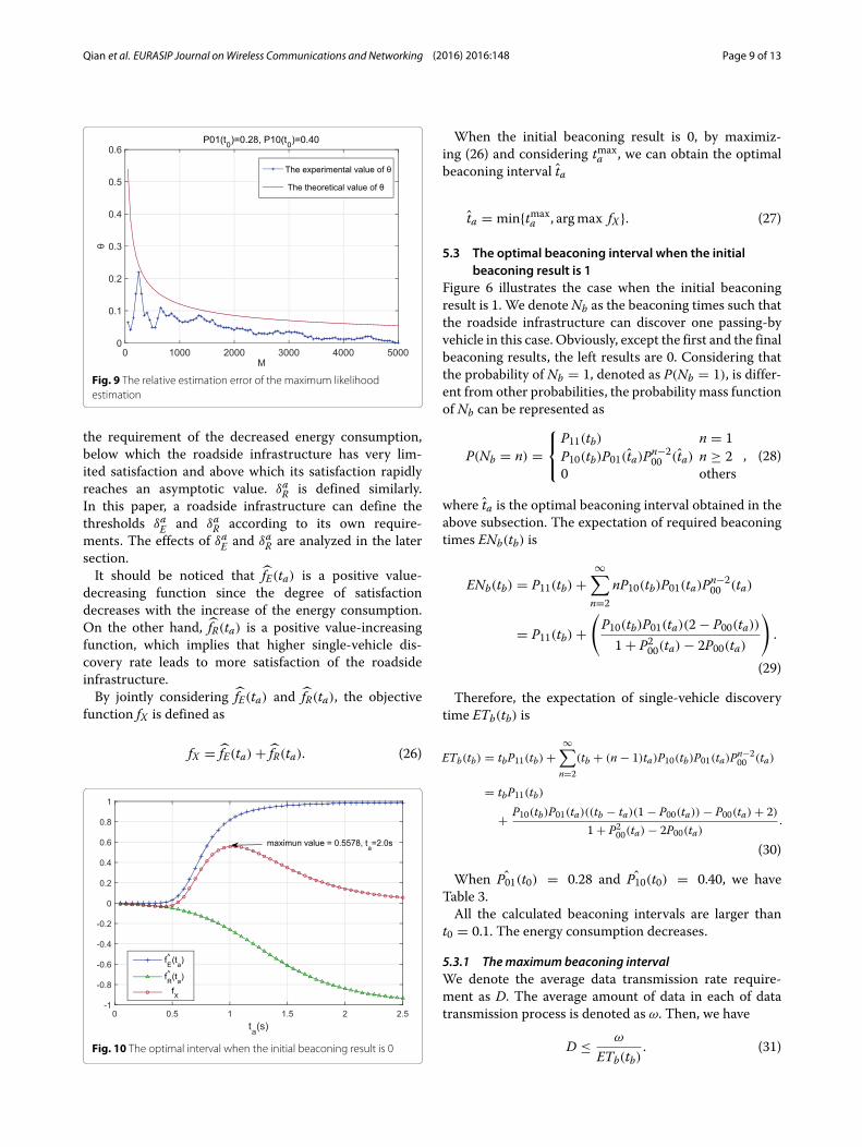
Fig. 9 The relative estimation error of the maximum likelihoodestimation

the requirement of the decreased energy consumption,below which the roadside infrastructure has very lim-ited satisfaction and above which its satisfaction rapidlyreaches an asymptotic value. δaR is defined similarly.In this paper, a roadside infrastructure can define thethresholds δaE and δaR according to its own require-ments. The effects of δaE and δaR are analyzed in the latersection.It should be noticed that fE(ta) is a positive value-

decreasing function since the degree of satisfactiondecreases with the increase of the energy consumption.On the other hand, fR(ta) is a positive value-increasingfunction, which implies that higher single-vehicle dis-covery rate leads to more satisfaction of the roadsideinfrastructure.By jointly considering fE(ta) and fR(ta), the objective

function fX is defined as

fX = fE(ta) + fR(ta). (26)

Fig. 10 The optimal interval when the initial beaconing result is 0

When the initial beaconing result is 0, by maximiz-ing (26) and considering tmax

a , we can obtain the optimalbeaconing interval ta

ta = min{tmaxa , argmax fX}. (27)

5.3 The optimal beaconing interval when the initialbeaconing result is 1

Figure 6 illustrates the case when the initial beaconingresult is 1. We denoteNb as the beaconing times such thatthe roadside infrastructure can discover one passing-byvehicle in this case. Obviously, except the first and the finalbeaconing results, the left results are 0. Considering thatthe probability of Nb = 1, denoted as P(Nb = 1), is differ-ent from other probabilities, the probability mass functionof Nb can be represented as

P(Nb = n) =⎧⎨⎩P11(tb) n = 1P10(tb)P01(ta)Pn−2

00 (ta) n ≥ 20 others

, (28)

where ta is the optimal beaconing interval obtained in theabove subsection. The expectation of required beaconingtimes ENb(tb) is

ENb(tb) = P11(tb) +∞∑n=2

nP10(tb)P01(ta)Pn−200 (ta)

= P11(tb) +(P10(tb)P01(ta)(2 − P00(ta))1 + P200(ta) − 2P00(ta)

).

(29)

Therefore, the expectation of single-vehicle discoverytime ETb(tb) is

ETb(tb) = tbP11(tb) +∞∑n=2

(tb + (n − 1)ta)P10(tb)P01(ta)Pn−200 (ta)

= tbP11(tb)

+ P10(tb)P01(ta)((tb − ta)(1 − P00(ta)) − P00(ta) + 2)1 + P200(ta) − 2P00(ta)

.

(30)

When ˆP01(t0) = 0.28 and ˆP10(t0) = 0.40, we haveTable 3.All the calculated beaconing intervals are larger than

t0 = 0.1. The energy consumption decreases.

5.3.1 Themaximumbeaconing intervalWe denote the average data transmission rate require-ment as D. The average amount of data in each of datatransmission process is denoted as ω. Then, we have

D ≤ ω

ETb(tb). (31)

Qian et al. EURASIP Journal onWireless Communications and Networking (2016) 2016:148 Page 10 of 13

According to (18), (19), and (20), we can calculate themaximum tb which is denoted as tmax

b .

5.3.2 The optimal beaconing intervalSimilarly, based on the Sigmoid function, we can obtainthe optimal beaconing interval as follows. We denotethe average decreased energy consumption as gE(tb). Theaverage decreased data rate is denoted as gR(tb). Then, wehave

gE(tb) = ξ

(ENb(t0)ETb(t0)

− ENb(tb)ETb(tb)

)(32)

gR(tb) = ω

(1

ETb(t0)− 1

ETb(tb)

). (33)

When the initial beaconing result is 1, we denote gE(tb)as the measure of the degree of satisfaction for thedecreased energy consumption, and we denote gE(tb) asthe Sigmoid function of fE(ta). δbE is a predefined thresholdreflecting the energy requirement, and δbR is a predefinedthreshold reflecting the data rate requirement. We denotegX as the objective function. Similar with the optimizationprocess in the above subsection, we have

gE(tb) = 1

1 + exp(−

(gE(tb) − δbE

)) (34)

gR(tb) = − 1

1 + exp(−

(gR(tb) − δbR

)) (35)

gX = gE(tb) + gR(tb). (36)

Then, we can obtain the optimal beaconing interval as tb

tb = min{tmaxb , argmax gX}. (37)

Through the above analyses, we can summarize thefollowing proposition:

Proposition 2. No matter the initial beaconing resultis 0 or 1, the optimal beaconing interval for the roadsideinfrastructure can be obtained by exploiting the tradeoffbetween the average energy consumption and the single-vehicle discovery rate.

5.4 Restarting the modeling processActually, the state transition probabilities are not con-stants.When they vary, the beaconing intervals previouslycalculated are no longer effective in the model. Some-times, keep using such intervals could lead to a sharpdecrease on single-vehicle discover rate. Thus, we need torestart the modeling phase to update the beaconing inter-vals after a certain period. Generally, there are two modesin real application, the first mode is to restart the mod-eling phase perodically. This mode is easy to implementby presetting a remodeling clock. The other mode is torestart the modeling phase on demand. We compare theexpected single-vehicle discovery rate with several recentobserved rates. If the difference is beyond a threshold andlasts for a particular length of time, we restart the mod-eling phase. This mode can better adapt to variability inthe model but also holds a higher computational complex-ity. In this paper, we do not specify which mode we apply.Research onmode selection and parameter determination

Fig. 11 The optimal interval when the initial beaconing result is 1

Qian et al. EURASIP Journal onWireless Communications and Networking (2016) 2016:148 Page 11 of 13

is not our focus in this paper. We leave it to the futurework.

6 Optimal beaconing interval in the datadissemination strategy

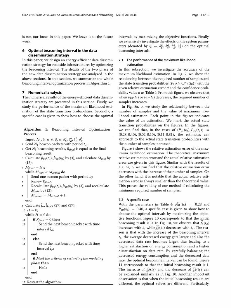
In this paper, we design an energy-efficient data dissemi-nation strategy for roadside infrastructures by optimizingthe beaconing interval. The details of the two phase ofthe new data dissemination strategy are analyzed in theabove sections. In this section, we summarize the wholebeaconing interval optimization process in Algorithm 1.

7 Numerical analysisThe numerical results of the energy-efficient data dissem-ination strategy are presented in this section. Firstly, westudy the performance of the maximum likelihood esti-mation of the state transition probabilities. Secondly, aspecific case is given to show how to choose the optimal

Algorithm 1: Beaconing Interval OptimizationProcessInput: N1, t0, α, θ , ξ , ω, δaE , δ

aR, δbE , δ

bR

1 Send N1 beacon packets with period t0;2 Get N1 beaconing results, Rfinal is equal to the finalbeaconing result;

3 Calculate p01(t0), p10(t0) by (3), and calculateMmin by(13);

4 Mfinal = N1;whileMmin < Mactual do

5 Send one beacon packet with period t0;6 Renew Rfinal;7 Recalculate p01(t0), p10(t0) by (3), and recalculate

Mmin by (13);8 Mactual = Mactual + 1;end

9 Calculate ta, tb by (27) and (37);10 H = 0;while H = 0 do

11 if Rfinal = 0 then12 Send the next beacon packet with time

interval ta;end

13 else14 Send the next beacon packet with time

interval tb;end

15 ifMeet the criteria of restarting the modelingphase then

16 H=1;end

end17 Restart the algorithm.

intervals by maximizing the objective functions. Finally,we extensively investigate the effects of the system param-eters (denoted by ξ , ω, δaE , δaR, δbE , δbR) on the optimalbeaconing intervals.

7.1 The performance of the maximum likelihoodestimation

In this subsection, we investigate the accuracy of themaximum likelihood estimation. In Fig. 7, we show therelationship between the required number of samples andthe state transition probabilities (P01(t0),P10(t0)) with thegiven relative estimation error θ and the confidence prob-ability value α as Table 4. From this figure, we observe thatwhen P01(t0) or P10(t0) decreases, the required number ofsamples increases.In Fig. 8a, b, we study the relationship between the

number of samples and the value of maximum like-lihood estimation. Each point in the figures indicatesthe value of an estimation. We mark the actual statetransition probabilities on the figures. In the figures,we can find that, in the cases of (P01(t0),P10(t0)) =(0.28, 0.40), (0.02, 0.10), (0.11, 0.81), the estimates canapproach to the actual state transition probabilities withthe number of samples increased.Figure 9 shows the relative estimation error of the max-

imum likelihood estimation. The theoretical maximumrelative estimation error and the actual relative estimationerror are given in this figure. Similar with the results ofFig. 8a, b, we can find that the relative estimation errordecreases with the increase of the number of samples. Onthe other hand, it is notable that the actual relative esti-mation error is always smaller than the theoretical value.This proves the validity of our method if calculating theminimum required number of samples.

7.2 A specific caseWith the parameters in Table 4, ˆP01(t0) = 0.28 andˆP10(t0) = 0.40, a specific case is given to show how to

choose the optimal intervals by maximizing the objec-tive functions. Figure 10 corresponds to that the initialbeaconing result is 0. In Fig. 10, we observe that fE(ta)increases with ta while fR(ta) decreases with ta. The rea-son is that with the increase of the beaconing intervalta, the average decreased energy gets larger and also thedecreased data rate becomes larger, thus leading to ahigher satisfaction on energy consumption and a higherdissatisfaction on data rate. By carefully balancing thedecreased energy consumption and the decreased datarate, the optimal beaconing interval can be found. Figure11 corresponds to that the initial beaconing result is 1.The increase of gE(tb) and the decrease of gR(tb) canbe explained similarly as in Fig. 10. Another importantobservation is that when the initial beaconing results aredifferent, the optimal values are different. Particularly,

Qian et al. EURASIP Journal onWireless Communications and Networking (2016) 2016:148 Page 12 of 13

a

b

c

Fig. 12 Effect of the system parameters when initially the state is 0. aEffects of ξ on fX . b Effects of ω on fX . c Effects of δaE , δ

aR on ta

when the maximum value of fX is 0.5578, the optimal bea-coning interval ta is 2 s; while when the maximum value ofgX is 0.8618, the optimal beaconing interval tb is 2.4 s.

Fig. 13 Effect of the system parameters when initially the state is 0.a Effects of ξ on gX . b Effects of ω on gX . c Effects of δbE , δ

bR on tb

7.3 Investigation on the effect of system parametersIn this subsection, we discuss the effect of parameters.Besides the parameters we discussed, the other parame-ters are set according to Table 2. Figure 12a–c illustratesthe simulation results when the initial beaconing result

Qian et al. EURASIP Journal onWireless Communications and Networking (2016) 2016:148 Page 13 of 13

is 0. Figure 12a shows the possible region of fX whenω = 300 kbit and ξ changes from 8.5 to 12mJ. Figure 12billustrates the influence of ω on the objective function fXwhen ξ = 10mJ. Since ξ affects the decreased energy con-sumption fE(ta), and ω is related to the decreased datarate fR(ta), the value of fX is affected by them. δaE andδaR are the thresholds when the initial beaconing resultis 0. δaE is a predefined threshold reflecting the energyrequirement, and δaR is a predefined threshold reflectingthe data rate requirement. Figure 12b shows the relation-ship between δaE , δaR, and ta. By adaptively adjusting thethreshold δaE and δaR, the roadside infrastructure can sat-isfy its various requirements. Specifically, if the roadsideinfrastructure prefers to work in an energy-saving mode,it can choose a long beaconing interval so as to save asmuch energy as possible. As shown in Fig. 12c, for a cer-tain δaE , the optimal beaconing interval ta increases withthe increase of δaR. On the contrary, if the roadside infras-tructure wants to disseminate more data, it can send thebeacon packets more frequently. Figure 13a–c illustratesthe simulation results when the initial beaconing result is1. The investigation is similar.

8 ConclusionsIn this paper, we propose an energy-efficient datadissemination strategy for roadside infrastructure inVCPS. We model the beaconing procedure in the datadissemination strategy as aMarkovmodel.With obtainingthe relationship between the beaconing interval and theexpectation of the single-vehicle discovery time, we cancalculate the maximum beaconing interval. By using theSigmoid function, we can obtain the optimal beaconinginterval to based on the satisfaction degree. The impactof the system parameters on the data dissemination strat-egy is investigated via extensive simulation study. Ourfuture work involves extensive empirical investigationsand analytical studies of the proposed approach.

Competing interestsThe authors declare that they have no competing interests.

AcknowledgementsThe authors would like to thank the support from the National Natural ScienceFoundation of China (Grant Nos. 61471028, 61371069, and 61272505).

Received: 31 December 2015 Accepted: 5 June 2016

References1. AA Cardenas, S Amin, S Sastry, in Proc. IEEE ICDCS. Secure control: towards

survivable cyber-physical systems, (2008), pp. 495–500. doi:10.1109/ICDCS.Workshops.2008.40

2. Y Huang, X Guan, Z Cai, T Ohtsuki, in 2013 IEEE International Conference onCommunications (ICC). Multicast capacity analysis for social-proximityurban bus-assisted VANETs, (2013), pp. 6138–6142. doi:10.1109/ICC.2013.6655586

3. J Shi, J Wan, H Yan, H Suo, in Proc. WCSP. A survey of cyber-physicalsystems, (2011), pp. 1–6. doi:10.1109/WCSP.2011.6096958

4. X Wang, L Guo, C Ai, J Li, Z Cai, in 8th International Conference, WASA 2013,Zhangjiajie, China, August 7-10, 2013. Proceedings. Wireless Algorithms,

Systems, and Applications (Springer Berlin Heidelberg, 2013),pp. 313–324. doi:10.1007/978-3-642-39701-1_26

5. X Li, X Yu, A Wagh, C Qiao, in Proc. IEEE INFOCOM. Human factors-awareservice scheduling in vehicular cyber-physical systems, (2011),pp. 2174–2182. doi:10.1109/INFCOM.2011.5935030

6. K Liu, VCS Lee, JK-Y Ng, J Chen, SH Son, Temporal data dissemination invehicular cyber x2013;physical systems. IEEE Transactions on IntelligentTransportation Systems. 15(6), 2419–2431 (2014). doi:10.1109/TITS.2014.2316006

7. X Zheng, Z Cai, J Li, H Gao, in Distributed Computing Systems (ICDCS), 2015IEEE 35th International Conference On. An application-aware schedulingpolicy for real-time traffic, (2015), pp. 421–430. doi:10.1109/ICDCS.2015.50

8. D Jia, K Lu, J Wang, X Zhang, X Shen, A survey on platoon-based vehicularcyber-physical systems. IEEE Communications Surveys Tutorials. PP(99),1–1 (2015). doi:10.1109/COMST.2015.2410831

9. J Gozalvez, M Sepulcre, R Bauza, IEEE 802.11p vehicle to infrastructurecommunications in urban environments. IEEE CommunicationsMagazine. 50(5), 176–183 (2012). doi:10.1109/MCOM.2012.6194400

10. A Paier, R Tresch, A Alonso, D Smely, P Meckel, Y Zhou, N Czink, in Proc.IEEE ICC. Average downstream performance of measured IEEE 802.11pinfrastructure-to-vehicle links, (2010), pp. 1–5. doi:10.1109/ICCW.2010.5503934

11. Y Huang, M Chen, Z Cai, X Guan, T Ohtsuki, Y Zhang, in 2015 IEEE GlobalCommunications Conference (GLOBECOM). Graph theory based capacityanalysis for vehicular ad hoc networks, (2015), pp. 1–5. doi:10.1109/GLOCOM.2015.7417561

12. Y Wang, J Zheng, N Mitton, in Proc. IEEE GLOBECOM. Delivery delayanalysis for roadside unit deployment in intermittently connectedVANETs, (2014), pp. 155–161. doi:10.1109/GLOCOM.2014.7036800

13. S Peirce, R Mauri, in Intell. Transp. Syst. Vehicle-infrastructure integration(VII) initiative benefit-cost analysis: pre-testing estimates (US DoT draftreport, Washington, DC, 2007)

14. M Kohvakka, M Hannikainen, TD Hamalainen, in 2005 IEEE 16thInternational Symposium on Personal, Indoor andMobile RadioCommunications. Energy optimized beacon transmission rate in awireless sensor network, vol. 2, (2005), pp. 1269–12732.doi:10.1109/PIMRC.2005.1651645

15. R Lasowski, C Linnhoff-Popien, Beaconing as a service: a novelservice-oriented beaconing strategy for vehicular ad hoc networks. IEEECommunications Magazine. 50(10), 98–105 (2012). doi:10.1109/MCOM.2012.6316782

16. A Daniel, DC Popescu, S Olariu, in Proc. IEE ICC. A study of beaconingmechanism for vehicle-to-infrastructure communications, (2012),pp. 7146–7150. doi:10.1109/ICC.2012.6364667

17. AA Hammad, GH Badawy, TD Todd, AA Sayegh, D Zhao, in Proc. IEEEGLOBECOM. Traffic scheduling for energy sustainable vehicularinfrastructure, (2010), pp. 1–6. doi:10.1109/GLOCOM.2010.5683759

18. AA Hammad, TD Todd, G Karakostas, D Zhao, Downlink traffic schedulingin green vehicular roadside infrastructure. IEEE Transactions on VehicularTechnology. 62(3), 1289–1302 (2013). doi:10.1109/TVT.2012.2227071

19. Z Yan, B Li, X Zuo, T Gao, in Proc. ICCVE. Fair downlink traffic scheduling forenergy sustainable vehicular roadside infrastructure, (2014),pp. 1092–1097. doi:10.1109/ICCVE.2014.7297519

20. S Mostofi, A Hammad, TD Todd, G Karakostas, in Proc. IEEE ICC. On/offsleep scheduling in energy efficient vehicular roadside infrastructure,(2013), pp. 6266–6271. doi:10.1109/ICC.2013.6655611

21. C Wen, J Zheng, in Proc. WCSP. An RSU on/off scheduling mechanism forenergy efficiency in sparse vehicular networks, (2015), pp. 1–5.doi:10.1109/WCSP.2015.7341227

22. AA Hammad, TD Todd, G Karakostas, Variable bit rate transmissionschedule generation in green vehicular roadside units. IEEE Transactionson Vehicular Technology. PP(99), 1–1 (2015). doi:10.1109/TVT.2015.2410798

23. Y Yao, L Rao, X Liu, X Zhou, in Proc. IEEE INFOCOM. Delay analysis andstudy of IEEE 802.11p based DSRC safety communication in a highwayenvironment, (2013), pp. 1591–1599. doi:10.1109/INFCOM.2013.6566955

24. S Bitam, A Mellouk, in Proc. IEEE VTC. Markov-history based modeling forrealistic mobility of vehicles in VANETs, (2013), pp. 1–5. doi:10.1109/VTCSpring.2013.6692628

25. X Chen, L Li, Y Zhang, A Markov model for headway/spacing distributionof road traffic. IEEE Transactions on Intelligent Transportation Systems.11(4), 773–785 (2010). doi:10.1109/TITS.2010.2050141