Embed Size (px)
Citation preview
University of Central Florida University of Central Florida
STARS STARS
Electronic Theses and Dissertations, 2004-2019
2015
Research on Improving Reliability, Energy Efficiency and Research on Improving Reliability, Energy Efficiency and
Scalability in Distributed and Parallel File Systems Scalability in Distributed and Parallel File Systems
Junyao Zhang University of Central Florida
Part of the Computer Sciences Commons, and the Engineering Commons
Find similar works at: https://stars.library.ucf.edu/etd
University of Central Florida Libraries http://library.ucf.edu
This Doctoral Dissertation (Open Access) is brought to you for free and open access by STARS. It has been accepted
for inclusion in Electronic Theses and Dissertations, 2004-2019 by an authorized administrator of STARS. For more
information, please contact [email protected].
STARS Citation STARS Citation Zhang, Junyao, "Research on Improving Reliability, Energy Efficiency and Scalability in Distributed and Parallel File Systems" (2015). Electronic Theses and Dissertations, 2004-2019. 5010. https://stars.library.ucf.edu/etd/5010
RESEARCH ON IMPROVING RELIABILITY, ENERGY EFFICIENCY AND SCALABILITYIN DISTRIBUTED AND PARALLEL FILE SYSTEMS
by
JUNYAO ZHANGM.S. Computer Science, University of Central Florida, 2010
M.E. Software Engineering, Jilin University, China 2009
A dissertation submitted in partial fulfilment of the requirementsfor the degree of Doctor of Philosophy
in the Department of Electrical Engineering and Computer Sciencein the College of Engineering and Computer Science
at the University of Central FloridaOrlando, Florida
Summer Term2015
Major Professor: Jun Wang

c© 2015 Junyao Zhang
ii
ABSTRACT
With the increasing popularity of cloud computing and “Big data” applications, current data cen-
ters are often required to manage petabytes or exabytes of data. To store this huge amount of data,
thousands or tens of thousands storage nodes are required ata single site. This imposes three major
challenges for storage system designers: (1) Reliability—node failure in these datacenters is a nor-
mal occurrence rather than a rare situation. This makes datareliability a great concern [68, 70]. (2)
Energy efficiency—a data center can consume up to100 times more energy than a standard office
building. More than 10% of this energy consumption can be attributed to storage systems. Thus,
reducing the energy consumption of the storage system is keyto reducing the overall consump-
tion of the data center. (3) Scalability—with the continuously increasing size of data, maintaining
the scalability of the storage systems is essential. That is, the expansion of the storage system
should be completed efficiently and without limitations on the total number of storage nodes or
performance.
This thesis proposes three ways to improve the above three key features for current large-scale
storage systems. Firstly, we define the problem of “reverse lookup”, namely finding the list of
objects (blocks) for a failed node. As the first step of failure recovery, this process is directly re-
lated to the recovery/reconstruction time. While existingsolutions use metadata traversal or data
distribution reversing methods for reverse lookup, which are either time consuming or expensive,
a deterministic block placement can achieve fast and efficient reverse lookup. However, the deter-
ministic placement solutions are designed for centralized, small-scale storage architectures such
as RAID etc.. Due to their lacking of scalability, they cannot be directly applied in large-scale
storage systems. In this paper, we propose Group-Shifted Declustering (G-SD), a deterministic
data layout for multi-way replication. G-SD addresses the scalability issue of our previous Shifted
Declustering layout and supports fast and efficient reverselookup.
iii
Secondly, we define a problem: “how to balance the performance, energy, and recovery in degrada-
tion mode for an energy efficient storage system?”. While extensive researches have been proposed
to tradeoff performance for energy efficiency under normal mode [23, 46, 15, 56], the system en-
tersdegradation modewhen node failure occurs, in which node reconstruction is initiated. This
very process requires a number of disks to be spun up and requires a substantial amount of I/O
bandwidth, which will not only compromise energy efficiencybut also performance. Without con-
sidering the I/O bandwidth contention between recovery andperformance, we find that the current
energy proportional solutions cannot answer this questionaccurately. This thesis present PERP,
a mathematical model to minimize the energy consumption fora storage systems with respect to
performance and recovery. PERP answers this problem by providing the accurate number of nodes
and the assigned recovery bandwidth at each time frame.
Thirdly, current distributed file systems such as Google File System(GFS) [49] and Hadoop Dis-
tributed File System (HDFS) [18], employ a pseudo-random method for replica distribution and a
centralized lookup table (block map) to record all replica locations. This lookup table requires a
large amount of memory and consumes a considerable amount ofCPU/network resources on the
metadata server. With the booming size of “Big Data”, the metadata server becomes a scalability
and performance bottleneck. While current approaches suchas HDFS Federation attempt to “hor-
izontally” extend scalability by allowing multiple metadata servers, we believe a more promising
optimization option is to “vertically” scale up each metadata server. We propose Deister, a novel
block management scheme that builds on top of a deterministic declustering distribution method
Intersected Shifted Declustering (ISD). Thus both replicadistribution and location lookup can be
achieved without a centralized lookup table.
iv

ACKNOWLEDGMENTS
This dissertation would not have been possible without the help and support of a number of people.
First and foremost, I would like to express my sincerest gratitude to my advisor, Dr. Jun Wang, for
the tremendous time, energy and wisdom he has invested in my graduate education. His inspiring
and constructive supervision has always been a constant source of encouragement for my study. I
also want to thank my dissertation committee members, Dr. Dan Marinescu, Dr. Cliff Zou and Dr.
Brian Goldiez, for spending their time to view the manuscript and provide valuable comments.
I would like to thank my past and current colleagues: Pengju Shang, Huijun Zhu, Qiangju Xiao,
Jiangling Yin, Xuhong Zhang, Ruijun Wang and Jian Zhou. I want especially thank to Jiangling
and Xuhong, for the inspiring discussion and continuous support to improve the quality of each
work. A special thanks to Jian, for tremendous help on my experiment setups. My gratitude also
goes to Huijun Zhu, who’s previous work provides great inspirations of this dissertation.
I dedicate this thesis to my family: my parents Yongxin Zhangand Yanfu Ma, my wife Lisa Li,
and my newborn baby Emmy Y. Zhang, for all their love and encouragement throughout my life.
Last but not least, I would also like to extend my thanks to my friends, who have cared and helped
me, in one way or another. My graduate studies would not have been the same without them.
v
TABLE OF CONTENTS
LIST OF FIGURES . . . . . . . . . . . . . . . . . . . . . . . . . . . . . . . . . . . . . .xi
LIST OF TABLES . . . . . . . . . . . . . . . . . . . . . . . . . . . . . . . . . . . . . . .xiii
CHAPTER 1: INTRODUCTION . . . . . . . . . . . . . . . . . . . . . . . . . . . . . .. 1
1.1 Achieving Fast Reverse Lookup using Scalable Deterministic Layout . . . . . . . . 2
1.2 Attacking the Balance among Energy, Performance and Recovery . . . . . . . . . 5
1.3 Deister: A Light-weighted Block Management Scheme in DiFS . . . . . . . . . . 9
CHAPTER 2: BACKGROUND . . . . . . . . . . . . . . . . . . . . . . . . . . . . . . . 12
2.1 Reverse Lookup Problem Assumptions and Backgrounds . . .. . . . . . . . . . . 12
2.1.1 Current Solutions for Reverse Lookup Problem . . . . . . .. . . . . . . . 13
2.2 Power Efficiency and Reliability in Storage Systems . . . .. . . . . . . . . . . . . 17
2.2.1 Energyvs.Reliability . . . . . . . . . . . . . . . . . . . . . . . . . . . . . 17
2.2.2 Reliabilityvs.Performance . . . . . . . . . . . . . . . . . . . . . . . . . . 18
2.2.3 Energyvs.Performance . . . . . . . . . . . . . . . . . . . . . . . . . . . 18
2.3 Block Management Schemes in Current DiFS . . . . . . . . . . . . .. . . . . . . 21
vi
2.3.1 Directory-based Mapping . . . . . . . . . . . . . . . . . . . . . . . .. . 21
2.3.2 Computational-based Mapping . . . . . . . . . . . . . . . . . . . .. . . . 22
2.3.2.1 Hashing . . . . . . . . . . . . . . . . . . . . . . . . . . . . . . 23
2.3.2.2 Deterministic Declustering . . . . . . . . . . . . . . . . . . .. 24
CHAPTER 3: GROUP-BASED SHIFTED DECLUSTERING . . . . . . . . . . . .. . . 25
3.1 Definitions and Notations . . . . . . . . . . . . . . . . . . . . . . . . . .. . . . . 26
3.2 Group-based Shifted declustering Scheme . . . . . . . . . . . .. . . . . . . . . . 28
3.3 Efficient Reorganization for Group Addition . . . . . . . . . .. . . . . . . . . . . 29
3.4 Group Addition Guideline . . . . . . . . . . . . . . . . . . . . . . . . . .. . . . 31
3.5 G-SD Distribution . . . . . . . . . . . . . . . . . . . . . . . . . . . . . . . .. . . 32
3.6 Optimal Group Size Configuration . . . . . . . . . . . . . . . . . . . .. . . . . . 32
3.7 G-SD Reverse Lookup . . . . . . . . . . . . . . . . . . . . . . . . . . . . . . .. 35
3.8 Analysis . . . . . . . . . . . . . . . . . . . . . . . . . . . . . . . . . . . . . . . .37
3.8.1 Reorganization Overhead Analysis . . . . . . . . . . . . . . . .. . . . . . 37
3.8.2 Analysis of Data Availability . . . . . . . . . . . . . . . . . . . .. . . . . 39
3.9 Evaluation . . . . . . . . . . . . . . . . . . . . . . . . . . . . . . . . . . . . . .. 43
3.9.1 Implementation on Ceph . . . . . . . . . . . . . . . . . . . . . . . . . .. 44
vii
3.9.2 Evaluation on Ceph . . . . . . . . . . . . . . . . . . . . . . . . . . . . . .45
3.9.2.1 I/O Throughput Test . . . . . . . . . . . . . . . . . . . . . . . . 46
3.9.2.2 Decentralized Metadata Traversingvs.G-SD Reverse Lookup . . 47
3.9.3 Implementation on HDFS . . . . . . . . . . . . . . . . . . . . . . . . . .47
3.9.4 Evaluation on HDFS . . . . . . . . . . . . . . . . . . . . . . . . . . . . . 49
3.9.4.1 I/O Performance Test . . . . . . . . . . . . . . . . . . . . . . . 49
3.9.4.2 Reverse Lookup Latency . . . . . . . . . . . . . . . . . . . . . 50
CHAPTER 4: PERFECT ENERGY, RECOVERY AND PERFORMANCE MODEL .. . 52
4.1 Problem Formulation . . . . . . . . . . . . . . . . . . . . . . . . . . . . . .. . . 52
4.1.1 Workload Model and Assumptions . . . . . . . . . . . . . . . . . . .. . . 52
4.1.2 The Energy Cost Model . . . . . . . . . . . . . . . . . . . . . . . . . . . 54
4.1.3 The PERP Minimization Problem . . . . . . . . . . . . . . . . . . . .. . 58
4.1.4 Solving PERP . . . . . . . . . . . . . . . . . . . . . . . . . . . . . . . . 60
4.2 PERP and Data Placement Schemes . . . . . . . . . . . . . . . . . . . . .. . . . 64
4.2.1 PERP Properties . . . . . . . . . . . . . . . . . . . . . . . . . . . . . . . 65
4.2.2 Applicability of Data Layout Schemes . . . . . . . . . . . . . .. . . . . 66
4.2.3 Selecting the Active Nodes . . . . . . . . . . . . . . . . . . . . . . .. . . 68
viii
4.3 Methodology . . . . . . . . . . . . . . . . . . . . . . . . . . . . . . . . . . . . .70
4.4 Experiments . . . . . . . . . . . . . . . . . . . . . . . . . . . . . . . . . . . . .. 73
4.4.1 PERP optimality . . . . . . . . . . . . . . . . . . . . . . . . . . . . . . . 73
4.4.1.1 PERPvs.Fixed recovery speedγ, varied active node numberx . 73
4.4.1.2 PERPvs.Fixed active node numberx, varied recovery speedγ . 75
4.4.2 Comparison between PERP, Maximum Recovery and Recovery Group . . 75
4.5 Conclusions . . . . . . . . . . . . . . . . . . . . . . . . . . . . . . . . . . . . .. 77
CHAPTER 5: DEISTER: A LIGHT-WEIGHT BLOCK MANAGEMENT SCHEME. . . 79
5.1 Overall Design . . . . . . . . . . . . . . . . . . . . . . . . . . . . . . . . . . .. 79
5.2 Intersected Shifted Declustering with Decoupled Address Mapping . . . . . . . . . 82
5.2.1 Block-to-node Mapping . . . . . . . . . . . . . . . . . . . . . . . . . .. 82
5.2.2 Reverse Lookup . . . . . . . . . . . . . . . . . . . . . . . . . . . . . . . 84
5.3 Load-aware Node-to-Group Mapping . . . . . . . . . . . . . . . . . .. . . . . . 85
5.4 Fast and Parallel Data Recovery . . . . . . . . . . . . . . . . . . . . .. . . . . . 87
5.5 Self-report Block Management . . . . . . . . . . . . . . . . . . . . . .. . . . . . 88
5.6 Evaluations . . . . . . . . . . . . . . . . . . . . . . . . . . . . . . . . . . . . .. 89
5.6.1 Testbed . . . . . . . . . . . . . . . . . . . . . . . . . . . . . . . . . . . . 89
ix

5.6.2 ISD Placementvs.Random Placement . . . . . . . . . . . . . . . . . . . . 90
5.6.3 ISD calculationvs.HDFS Block Map Lookup . . . . . . . . . . . . . . . 91
5.6.4 Memory Space . . . . . . . . . . . . . . . . . . . . . . . . . . . . . . . . 92
CHAPTER 6: CONCLUSION . . . . . . . . . . . . . . . . . . . . . . . . . . . . . . . .93
APPENDIX : PROOF OF REORGANIZATION OVERHEAD . . . . . . . . . . . . .. 95
LIST OF REFERENCES . . . . . . . . . . . . . . . . . . . . . . . . . . . . . . . . . . .101
x
LIST OF FIGURES
1.1 Research Work Overview . . . . . . . . . . . . . . . . . . . . . . . . . . . .2
1.2 Average percentage of operation time to stay in degradation mode . . . . . . 7
3.1 Example of Shifted Declustering Layout with total number of 9 nodes . . . . 25
3.2 Example of Shifted Declustering Layout with total number of 6 nodes . . . . 26
3.3 Group-SD Scheme . . . . . . . . . . . . . . . . . . . . . . . . . . . . . . . 29
3.4 The Procedure of “Lazy Node Addition Policy” . . . . . . . . . .. . . . . . 31
3.5 Reorganization overhead Comparison . . . . . . . . . . . . . . . .. . . . . 39
3.6 The comparison ofP (k) between G-SD and Random Distribution . . . . . . 42
3.7 Throughput Comparison between G-SD and Ceph CRUSH . . . . .. . . . . 46
3.8 Average response latency comparison between G-SD RL andDMT on Ceph 48
3.9 Execution time comparison between G-SD and HDFS defaultrandom layout . 50
3.10 RL time comparison between G-SD RL and HDFS Tree-Reversing (TR) . . 51
4.1 Illustration of start point, end point time scales . . . . .. . . . . . . . . . . 53
4.2 Recovery illustration with non-overlapping nodes and overlapping nodes . . . 61
4.3 Illustration of Optimal Solutions of Financial I trace .. . . . . . . . . . . . . 64
xi
4.4 Example of 9-node Group-rotational Declustering Layout . . . . . . . . . . . 67
4.5 Case study of finding the active nodes in group rotationallayout . . . . . . . 70
4.6 Comparisons of Performance and power consumption with fixedx and variedγ 74
4.7 Comparisons between PERP, MR and RG when recovering 240GB data . . . 76
4.8 Comparisons between PERP, MR and RG when recovering 320GB data . . . 77
5.1 Metadata management method in HDFS, a typical DiFS . . . . .. . . . . . . 80
5.2 Proposed metadata management solution . . . . . . . . . . . . . .. . . . . . 80
5.3 Example of block-to-bode mapping . . . . . . . . . . . . . . . . . . .. . . . 84
5.4 Example of Reverse Lookup . . . . . . . . . . . . . . . . . . . . . . . . . .85
5.5 Example of Parallel reconstruction . . . . . . . . . . . . . . . . .. . . . . . 88
5.6 Performance Comparison between ISD and random . . . . . . . .. . . . . . 90
5.7 Performance Comparison of Locating one block . . . . . . . . .. . . . . . . 91
5.8 Memory space cost for block-to-node mapping . . . . . . . . . .. . . . . . 92
xii
LIST OF TABLES
2.1 Comparison between Existing Reverse Lookup Solutions .. . . . . . . . . . 16
2.2 Comparison among block-to-node mapping schemes . . . . . .. . . . . . . 22
3.1 Summary of Notation . . . . . . . . . . . . . . . . . . . . . . . . . . . . . . 27
4.1 Notation summary . . . . . . . . . . . . . . . . . . . . . . . . . . . . . . . . 53
4.2 Summary of PERP adaptability study . . . . . . . . . . . . . . . . . .. . . 66
4.3 CASS Cluster Configuration . . . . . . . . . . . . . . . . . . . . . . . . .. 71
5.1 Summary of Notation . . . . . . . . . . . . . . . . . . . . . . . . . . . . . . 82
xiii
CHAPTER 1: INTRODUCTION
We are now entering the era of “Big Data”, in which mountains of data are generated and analyzed
every day by both scientific and industry applications. In astronomy, Sloan Digital Sky has stored
data for 215 million unique objects and they are still growing [12]; in geophysics, billions of photos
are captured of earth’s surface to the sun and it is still growing [4]. Facebook [5] is generating
55,000 images per second at peak usage [57], all of which require storage of the data. Under these
circumstances, system designers are developing ever-larger storage systems to meet the exploding
demands of data storage. These petabyte(exa)-scale data clusters usually consist of thousands or
tens of thousands of storage nodes.
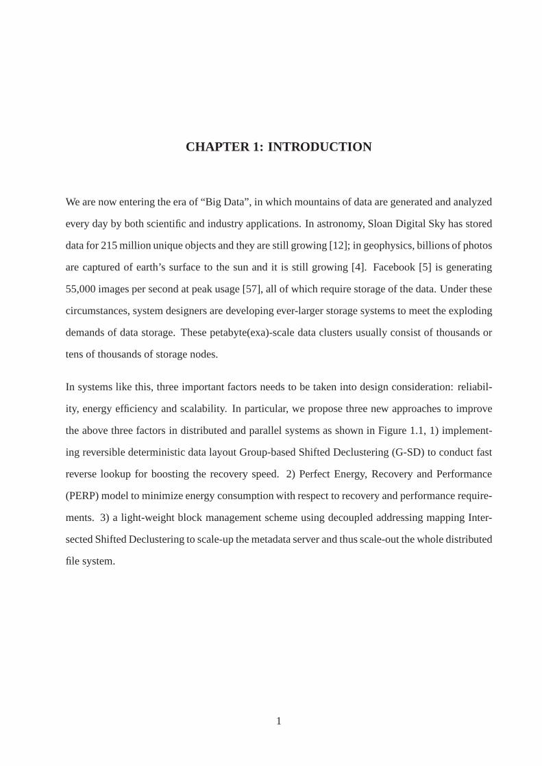
In systems like this, three important factors needs to be taken into design consideration: reliabil-
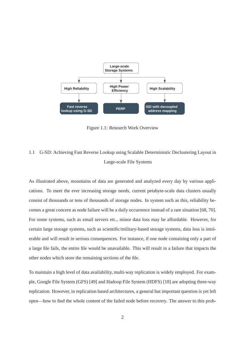
ity, energy efficiency and scalability. In particular, we propose three new approaches to improve
the above three factors in distributed and parallel systemsas shown in Figure 1.1, 1) implement-
ing reversible deterministic data layout Group-based Shifted Declustering (G-SD) to conduct fast
reverse lookup for boosting the recovery speed. 2) Perfect Energy, Recovery and Performance
(PERP) model to minimize energy consumption with respect torecovery and performance require-
ments. 3) a light-weight block management scheme using decoupled addressing mapping Inter-
sected Shifted Declustering to scale-up the metadata server and thus scale-out the whole distributed
file system.
1
Large-scale Storage Systems
High Reliability High Power Efficiency High Scalability
Fast reverse lookup using G-SD PERP ISD with decoupled
address mapping
Figure 1.1: Research Work Overview
1.1 G-SD: Achieving Fast Reverse Lookup using Scalable Deterministic Declustering Layout in
Large-scale File Systems
As illustrated above, mountains of data are generated and analyzed every day by various appli-
cations. To meet the ever increasing storage needs, currentpetabyte-scale data clusters usually
consist of thousands or tens of thousands of storage nodes. In system such as this, reliability be-
comes a great concern as node failure will be a daily occurrence instead of a rare situation [68, 70].
For some systems, such as email servers etc., minor data lossmay be affordable. However, for
certain large storage systems, such as scientific/military-based storage systems, data loss is intol-
erable and will result in serious consequences. For instance, if one node containing only a part of
a large file fails, the entire file would be unavailable. This will result in a failure that impacts the
other nodes which store the remaining sections of the file.
To maintain a high level of data availability, multi-way replication is widely employed. For exam-
ple, Google File System (GFS) [49] and Hadoop File System (HDFS) [18] are adopting three-way
replication. However, in replication based architectures, a general but important question is yet left
open—how to find the whole content of the failed node before recovery. The answer to this prob-
2
lem is the key to recover the missing data or reconstructing the failed node. We call this specific
process asreverse lookup (RL). We define reverse lookup by considering it as an inverse process
to data distribution. While data distribution methods attempt to locate the storage nodes for one
piece of data, the RL process aims to locate all of the data given a failed node ID.
The current solutions to RL problem can be divided into threecategories—metadata traversing,
data distribution reversing and deterministic data layoutreversing. The major limitations of these
approaches are listed below. For simplicity, we use the term“object” to symbolize a data unit such
as “block” or “chunk” in different systems and the term “node” to symbolize a “storage server”.
Metadata traversingMetadata traversing is widely adopted by current parallel and distributed file
systems such as Ceph [61], Vesta [24], Panasas [63] etc. Whena node failure occurs and a timeout
is detected by the metadata server, it will fire up a process that finds the object list by traversing its
whole index node (inode) table. The fundamental problem with this approach is that finding the
list of one node requires traversing the whole inode table, which is expensive and time consuming.
Scalable data distribution reversingSince RL is the exact reverse process of data distribution,
a more efficient solution is to locate the content by reversing the data distribution algorithms,
which can avoid the inefficient and time consuming traversing process. However, existing scalable
data distribution algorithms include table based (hierarchical lookup table) approaches [55, 18],
and computation based (pure hashing) approaches [61, 20]. Table based approach can achieve
reverse lookup but has limited scalability, while the hashing functions are typically irreversible.
Deterministic data layout reversingDeterministic data layout is developed to place replicas on
different nodes to achieve high reliability in a replication/parity based architecture. Representatives
are chained declustering [30], group-rotational declustering [22], and shifted declustering [77, 52].
In these schemes, RL can be well supported because the placement algorithms are pre-computed
and the distribution algorithm is reversible. However, in these systems, the object locations depend
on the total number of nodes. Thus when the system expands, adding storage nodes into an already
3

balanced layout will result in heavy data reorganization.
We proposeGroup-based Shifted Declustering (G-SD) layout, a scalable placement-ideal layout
that leverages the scalability issues for our previously developed deterministic layout—Shifted
Declustering(SD) [77]. The main idea is to take advantage ofthe support for fast and efficient
reverse lookup in the deterministic layout; and addresses its scalability issue. More specifically, G-
SD limits the reorganization overhead into a reasonable level such that SD can be extended into the
large scale file system. The preliminary design and simulation results are presented in my master
thesis [71]. This work continues the existing project and makes the followingnew contributions:
• We present a new practical design of G-SD distribution, namely, to distribute the data with
the awareness of G-SD groups utilization.
• We study the new method of reverse lookup in HDFS tree-reversing, which builds a quick
index in its block map. Even though recovery may not be time-sensitive, reverse lookup is
still an important in terms of metadata integrity. The namenode must locates the missing
blocks when node failure occurs as soon as possible. Comparison results are presented
showing that G-SD reverse lookup outperforms this approach. Also, we studied the reverse
lookup problem by incorporating a new category: deterministic data layout, which includes
centralized deterministic layout schemes and Group-basedShifted Declustering.
• We research a simple yet effective method to strike the tradeoff for determining the optimal
size of each group. Instead of considering the tradeoff between reorganization overhead and
recovery speed, we believe that a better approach to consider the optimal group size for a
stable group to tradeoff between recovery speed and failurerate. This is because most of the
the groups do not need to reorganize when system expansion occurs, for which the optimal
group size for a group does not need to consider reorganization overhead.
4
• We study the data layout impact on data availability by quantifying the most important pa-
rameter “probability of not losing data afterl nodes fail”. Compared with the random distri-
bution (varies between0%−99.9999%), the G-SD layout is able to maintain high and steady
availability (99.8%− 99.9999%).
• We completely redo the experiment section. Instead of usingsimulation results on PVFS2 as
shown in [71], we implement the prototype of the G-SD layout and its reverse lookup func-
tion in two open-source distributed file systems: Ceph and HDFS. Implementation of G-SD
on Ceph is done inCRUSH module, in which CRUSH map but substitute the CRUSH
distribution algorithm with G-SD [62]. Implementation on HDFS is done solely on namen-
ode. More specifically, we extend the BlockPlacementPolicyinterface to modify the layout
mechanism. Evaluations of G-SDs impact on HDFS normal performance and RL lookup
speed are presented. A new indication from experiment results is shown that G-SD RL is
able to achieve better speedup with a larger scale experiment. Evaluation results collected
on PRObE Marmot clusters [7, 64] show that the average speed of G-SD reverse lookup is
over one order of magnitude faster that the existing metadata traversal and tree-reversing
methods. Moreover, the gap will continue increase with the growth of data size.
1.2 PERP: Attacking the Balance among Energy, Recovery and Performance in Storage Systems
Energy consumption of data centers has become a major concern with the consistent increase of
online services and cloud computing. Among all of the devices, energy consumption by the disk-
based storage subsystems takes a substantial fraction to keep thousands or tens of thousands of
disks spinning. It is reported that the storage devices contributed more than 10% of the data centers’
total power consumption [34]. Moreover, storage energy consumption may easily surpass the
energy consumed by the rest of the computing systems [46, 78]and this percentage will continue to
5
grow, as data center expands with the increasing demand of storage capacity. Thus, it is imperative
to develop energy-efficient and high-performance storage systems to increase the revenue of data
center operators and promote environmental conservation,without violating the Quality of Service
(QoS) [11].
To address this problem, extensive research has been conducted for the purpose of saving energy
with a reasonable performance tradeoff. For example, Dynamic Rotations Per Minute (DRPM) [28]
can allowed disks to switch to a lower-energy state while serving requests with lower performance.
Massive array of inexpensive disks (MAID) [23] and Popularity Data Concentration (PDC) [46]
skew popular data into either some cache disks or a subset of disks, which serves requests with
a lower performance while the other disks can be spun down to conserve energy. Most recently,
Barrosoet al [17] from Google presented an important metric called “energy proportional”, which
argued that the energy consumption should be in proportion to the system utilization/performance.
In a storage system, the implies that the total number of active disks should be proportional to
the total I/O throughput. Since the workload on the storage system is location-dependent, apply-
ing this metric in a storage system is closely related to the data layouts. As such, several power
proportional data layouts for storage systems are proposed, such as Rabbit [15] for distributed file
systems and Sierra [56] for web servers.
However, this tradeoff metric is only defined for normal modewhere the system is functioning
normally without any node failures. When node failure occurs, the storage system enters the
degradation mode(for online recovery), in which node reconstruction is initialized. This process
needs to spin up a number of disks. Furthermore, Furthermore, node reconstruction requires a
substantial amount of I/O bandwidth, which creates a contention between the performing the re-
covery process and normal services. Hence both energy efficiency and normal performance will
be compromised. The following problem arises: how to balance the performance, energy, and
reliability in this degradation mode for an energy efficientstorage system? One may argue that the
6
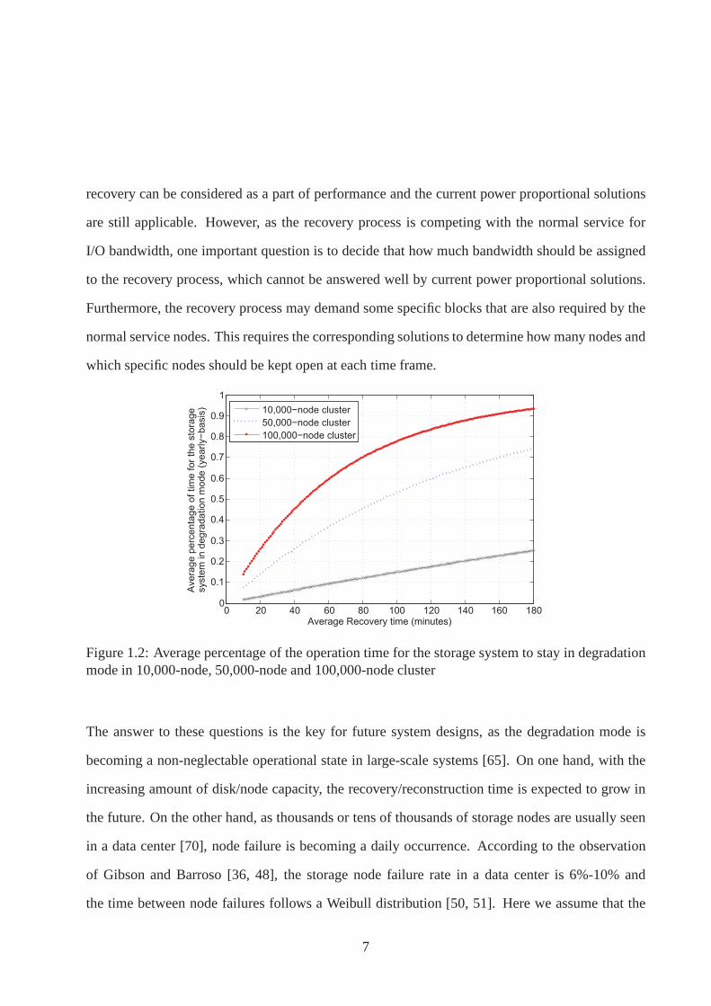
recovery can be considered as a part of performance and the current power proportional solutions
are still applicable. However, as the recovery process is competing with the normal service for
I/O bandwidth, one important question is to decide that how much bandwidth should be assigned
to the recovery process, which cannot be answered well by current power proportional solutions.
Furthermore, the recovery process may demand some specific blocks that are also required by the
normal service nodes. This requires the corresponding solutions to determine how many nodes and
which specific nodes should be kept open at each time frame.
0 20 40 60 80 100 120 140 160 1800
0.1
0.2
0.3
0.4
0.5
0.6
0.7
0.8
0.9
1
Average Recovery time (minutes)
Avera
ge p
erc
enta
ge o
f tim
e f
or
the s
tora
ge
syste
m in d
egra
dation m
ode (
yearly−
basis
) 10,000−node cluster
50,000−node cluster
100,000−node cluster
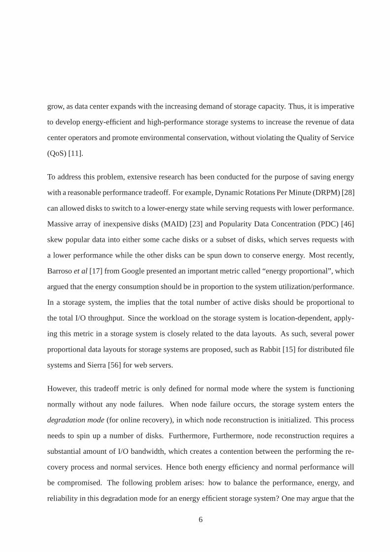
Figure 1.2: Average percentage of the operation time for thestorage system to stay in degradationmode in 10,000-node, 50,000-node and 100,000-node cluster
The answer to these questions is the key for future system designs, as the degradation mode is
becoming a non-neglectable operational state in large-scale systems [65]. On one hand, with the
increasing amount of disk/node capacity, the recovery/reconstruction time is expected to grow in
the future. On the other hand, as thousands or tens of thousands of storage nodes are usually seen
in a data center [70], node failure is becoming a daily occurrence. According to the observation
of Gibson and Barroso [36, 48], the storage node failure ratein a data center is 6%-10% and
the time between node failures follows a Weibull distribution [50, 51]. Here we assume that the
7
annual failure rate of a node is 8%, we run a Monte Carlo simulation to measure the average time
percentages of the storage system that stays in the degradation mode with various recovery time. As
shown in Figure 1.2, the percentage of time spent in the degradation mode increases significantly
with the growing size of the data cluster.e.g. when the recovery time is40 minutes, this time
percentage increases from8% for a10, 000-node cluster to44% for a100, 000-node cluster.
Moreover, with three-way replication in current main-stream storage, more systems are inclin-
ing to adopt a “lazy recovery” scheme, which recovers the failed blocks based on the replication
threshold [18]. If the replica number for a block is still above the threshold, it will be recovered
at a relatively slower speed, and vice versa. This provides us an opportunity to reduce the en-
ergy consumption while satisfying both performance and recovery requirements. In this thesis, we
present a mathematical model called Perfect Energy, Recovery and Performance (PERP) [73, 74]
to help system designers balance the relationship among these three key characteristics, which
aims to minimize the energy cost based on certain performance and recovery constraints. PERP
dynamically adjusts the number of active nodes and the corresponding recovery speed. We then
study the adaptability of PERP on current well-accepted power proportional data layouts. Fur-
thermore, to better apply PERP in practice, we propose a new node selection algorithm GIA to
help choose nodes according to PERP’s results. Finally we validate the effectiveness of PERP by
comparing it with the maximum recovery scheme abstracted from Sierra, and the recovery group
scheme abstracted from Rabbit. Experimental results validate that our model outputs are optimal
and can achieve a considerable amount of energy savings while satisfying all of the performance
and recovery requirements.
8

1.3 Deister: A Light-weighted Block Management Scheme in Data-intensive File Systems
using Scalable Deterministic Declustering Distribution
In the era of “Big Data”, these vast amount of data are analyzed by both scientists and Inter-
net companies to make scientific discoveries and study business trends etc. [2]. To speedup this
analysis process, data-intensive computing frameworks are proposed, in which computation job
tasks are scheduled to the data locations due to the large data set,i.e. MapReduce Framework.
Accompanied with this framework, a dedicated storage architecture, featured as high-throughput,
highly-reliably and cost-effective, is designed to provide high performance for these type of jobs.
We refer this storage architecture asData-intensive File System (DiFS). Leading representatives
such as GFS [49] and HDFS [18], Quantcast File System (QFS) [45] are defined as this purpose-
built paradigm.
Current DiFS adopt a master-slave architecture and is builton top of the local file system, where
all the metadata is managed by the master nodes and the physical data is managed by the lo-
cal file systems on the slave (data) nodes. To maintain high availability, files are divided into
fixed-sized blocks (or chunks), which are replicated (usually three-way) and distributed pseudo-
randomly across the cluster with the consideration of the rack-awareness. To track these randomly
distributed replicas, the master nodes store the locationsof all blocks. Moreover, to guarantee
the consistency between the stored location information and the physical data, the master nodes
receive periodical updates from the slave nodes, includingblock reports and heartbeats. We refer
these management scheme asDiFS block management(block management for simplicity in the
rest of this paper). This scheme offers great flexibility because each block is placed correlation-
free. However, this comes with a high cost in terms of memory and maintenance.
• Memory cost: the locations information of each block is required to be stored in the memory
of the master server, which can be referred as theblock map. This block map costs a large
9
proportion of the total memory taken by DiFS master node. It is observed that on each
master node, with a file-to-block ratio of1 : 1, the block map takes more than40% of the
total used memory; and the proportion will reach more than60% with a file-to-block ratio of
1 : 5 [13, 53].
• Maintenance cost: as the physical replicas are managed in the local file systemon the slave
nodes, the block management scheme requires a high cost on the master server’s CPU and
network bandwidth to synchronize the block map with the actual scenarios on the slaves
nodes [13]. For example, in a10, 000-node cluster with a storage capacity of60 PB (file
to block ratio is1 : 1.5) [53], 30% of the namenode’s total processing capacity is used to
process the block reports.
With the continuously increasing size of data, these cost becomes non-negligible, causing the mas-
ter node to become a scalability and performance bottleneckdue to its hardware bound of the
master node’s memory heap size and processing capability. To address this bottleneck, Namenode
(master node) Federation [1] is proposed to split the singlemaster node into manyindependent
master nodes and thus allows the metadata management to scale “horizontally”. While this ap-
proach is able to reduce the amount of memory taken on each master node and provide a work-
ing DiFS, we believe a more promising optimization option isto “vertically” scaleeach master
node—to improve the performance and scalability of each master node. More specifically, this can
be achieved by reducing the memory and maintenance cost of the block management module. For
example, the scalability of a DiFS can easily be doubled whenthe block map is separated from the
master node. To achieve this, standalone block management is proposed by aY ahoo! team, which
aims to move the block management module out of the master node to some dedicated block man-
agement(BM) nodes [13]. With the memory and maintenance cost reduced on each master node,
this approach may slow down the metadata lookup operations because an extra hop of network
lookup is introduced.
10

In this project, we propose Deister, an alternative light-weighted block management scheme that
can offers the same read/write speed and reliability; but much faster metadata lookup speed, lower
memory cost and much lower internal workloads on the master server. Deister consists of a deter-
ministic block distribution algorithm Intersected Shifted Declustering (ISD) and its corresponding
metadata management schemes, including calculable block lookup and self-reporting block report.
The basic idea of Deister is to distribute the data deterministically based on a reversible mathemat-
ical function so that each block location can be calculated,thus allowing the centralized/decentral-
ized block locations to be removed. Moreover, the block report is offloaded to datanodes—based
on the revere function of ISD, the block list of a certain nodecan also be calculated, which can
be compared with the generated block report for further operations. In this way, the two largest
overhead of block management, memory spaces and internal workloads, can be minimized. Our
results show that the placement policy has the identical I/Othroughput with the HDFS default ran-
dom layout, while the memory space saving on the metadata node is63% in a 1024-node cluster
with 500 million blocks.
11

CHAPTER 2: BACKGROUND
In this chapter, we discuss the current solutions and their limitations for the reverse lookup problem
and storage power management.
2.1 Reverse Lookup Problem Assumptions and Backgrounds
Based on our investigation and to the best of our knowledge, the reverse lookup problem has not
been widely studied. Partially because in some cases, this problem is not vital. In Peer-to-Peer
(P2P) systems such as Chord [54] and Kademlia [44], there is no need to recover or reconstruct
the node when node failure happens because they are assumed insecure and employed high degree
of replications. Most of these systems make little attempt to guarantee long persistence of stored
objects because nodes are added and removed frequently. Losing one node simply means to lose
access to the data store on that node while other nodes are maintaining the same data and would
be able to provide query services. For example, Kademlia [44] keepsk replicas, which is usually
set to 20, for one file. Under these circumstances, recovery and reverse lookup is unnecessary.
For some other systems such as Google File System (GFS) [49] or Hadoop File System (HDFS) [18],
fast reverse lookup is important in terms ofmetadata integrity rather than recovery time. These
systems adopt a “lazy (passive) recovery” scheme. A certainthreshold for block replicas is main-
tained on the Metadata Server (MDS). When the number of replicas for certain blocks are lower
than the predetermined threshold (which may be resulted from node failure), the system will ini-
tiate a re-replication for the missing chunk(s). In this case, recovering the missing blocks is not
time-sensitive if the replication threshold is not set as high the replica number. However, a fast re-
verse lookup is still required because the metadata serversneed to locate the missing blocks within
its inode entries and update (replicationnumber− 1) the number of the existing replications. It is
12

critical that this process is completed as soon as possible so to keep the consistency of the metadata
with the status of the data node; and furthermore the re-replication is conducted on time.
The reverse lookup problem resides in the system that follows the basic assumptions below:
1. The file system is at least a petabyte-scale storage system, which contains thousands to tens
of thousands of storage nodes. Each node holds a large numberof data objects. Objects are
relatively large in terms of tens of megabytes to several gigabytes.
2. The storage servers and clients are tightly connected: this is different from the loosely con-
nected architecture such as peer-to-peer networks where communication latency varies from
node-to-node.
3. The system has a high requirement of system reliability and data availability.
4. A k-way replication scheme is employed, which means that each piece of data is copiedk
times to keep up the availability and reliability.
2.1.1 Current Solutions for Reverse Lookup Problem
As mentioned in Chapter 1, there are three basic solutions for the Reverse Lookup problem: meta-
data traversing, data distribution reversing and deterministic layout reversing.
Metadata traversal Metadata traversing approaches vary among different metadata management
schemes. Existing metadata management approaches can be divided into two categories: central-
ized and decentralized metadata management. In centralized metadata management systems, such
as Lustre [19], the whole namespace are maintained in one or duplicated on multiple metadata
servers (for passive failover). Reverse lookup process is able to be conducted by traversing the
13
whole inode table—suppose the system wants to construct theblock list i, the operation is “find
the inode which has the owner IDi”.
In decentralized metadata management schemes, the system distributes the file metadata into mul-
tiple MDSs using different strategies, such as table-basedmapping [55], hash-based mapping [62],
static-tree based mapping, dynamic-tree based mapping andbloom filter-based mapping [79]. As
file metadata from the same node could be distributed into different MDSs, the decentralized meta-
data management scheme divided the system namespace into multiple parts. In this way, metadata
queries and workloads are shared so that the central bottleneck can be effectively avoided. In case
of the above example, to retrieve the object list for nodei, all metadata from every MDSs are
needed to be examined and the result from each MDS has to be pieced together.
For both architectures, this traversing process significantly increases the recovery time because
examining such a large amount of metadata for a petabyte-scale system will take a long time. Even
though parallel discovery in decentralized metadata management systems may be introduced to
reduce the lookup time, piecing the on-node data structuresback together will take considerable
time. To make things worse, this time consuming process alsoincreases the probability of data
loss due to the fact that other nodes may fail during the time of traversing and examining the meta-
data. As stated in paper [55], file systems of petabyte-scaleand complexity cannot be practically
recovered by one process, which examines the file system metadata to reconstruct the file system.
This long lookup time makes this scheme not suitable for fastrecovery.
Scalable Data Distribution Reversing A more reasonable solution for reverse lookup is to reverse
the process of data distribution algorithms, which aims to provide the proper location for a piece of
data. i.e. RUSH [29] is a decentralized data distribution algorithm that can map replicated objects
to a scalable collection of storage servers. Data distribution approaches could also be divided into
two categories: centralized control (table based) and decentralized control.
14
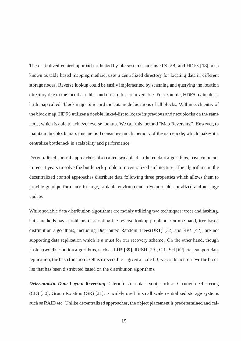
The centralized control approach, adopted by file systems such as xFS [58] and HDFS [18], also
known as table based mapping method, uses a centralized directory for locating data in different
storage nodes. Reverse lookup could be easily implemented by scanning and querying the location
directory due to the fact that tables and directories are reversible. For example, HDFS maintains a
hash map called “block map” to record the data node locationsof all blocks. Within each entry of
the block map, HDFS utilizes a double linked-list to locate its previous and next blocks on the same
node, which is able to achieve reverse lookup. We call this method “Map Reversing”. However, to
maintain this block map, this method consumes much memory ofthe namenode, which makes it a
centralize bottleneck in scalability and performance.
Decentralized control approaches, also called scalable distributed data algorithms, have come out
in recent years to solve the bottleneck problem in centralized architecture. The algorithms in the
decentralized control approaches distribute data following three properties which allows them to
provide good performance in large, scalable environment—dynamic, decentralized and no large
update.
While scalable data distribution algorithms are mainly utilizing two techniques: trees and hashing,
both methods have problems in adopting the reverse lookup problem. On one hand, tree based
distribution algorithms, including Distributed Random Trees(DRT) [32] and RP* [42], are not
supporting data replication which is a must for our recoveryscheme. On the other hand, though
hash based distribution algorithms, such as LH* [39], RUSH [29], CRUSH [62] etc., support data
replication, the hash function itself is irreversible—given a node ID, we could not retrieve the block
list that has been distributed based on the distribution algorithms.
Deterministic Data Layout Reversing Deterministic data layout, such as Chained declustering
(CD) [30], Group Rotation (GR) [21], is widely used in small scale centralized storage systems
such as RAID etc. Unlike decentralized approaches, the object placement is predetermined and cal-
15
culated by a certain reversible algorithm on the RAID controller, which makes RL feasible on these
deterministic data layouts. Moreover, the placement-ideal deterministic placement algorithm—
Shifted Declustering, satisfies the following properties [77]:1)Multiple Failures Correcting: a k-
way (k ≥ 2) replication architecture should provide(k − 1) failures correction. 2)Distributed
Replica Information: if we distinguish data between primary copies and secondary copies (repli-
cas), each node should hold the same number of replicas to satisfy this property. But this property
is satisfied by nature if the copies are equally important. 3)Distributed reconstruction: the work-
load that is supposed to be handled by the failed node will be dispatched evenly to all the surviving
nodes. 4)Large Write Optimization: requires writing a large number of continuous units without
pre-reading units for updating checksum information. It issatisfied in all replication-based archi-
tectures. 5)Maximal Parallelism: requires to access at most⌈o/n⌉ addresses from each node is
accessed wheno consecutive addresses is accessed. 6)Efficient Mapping: requires that the func-
tions that map client addresses to node system locations areefficiently computable.
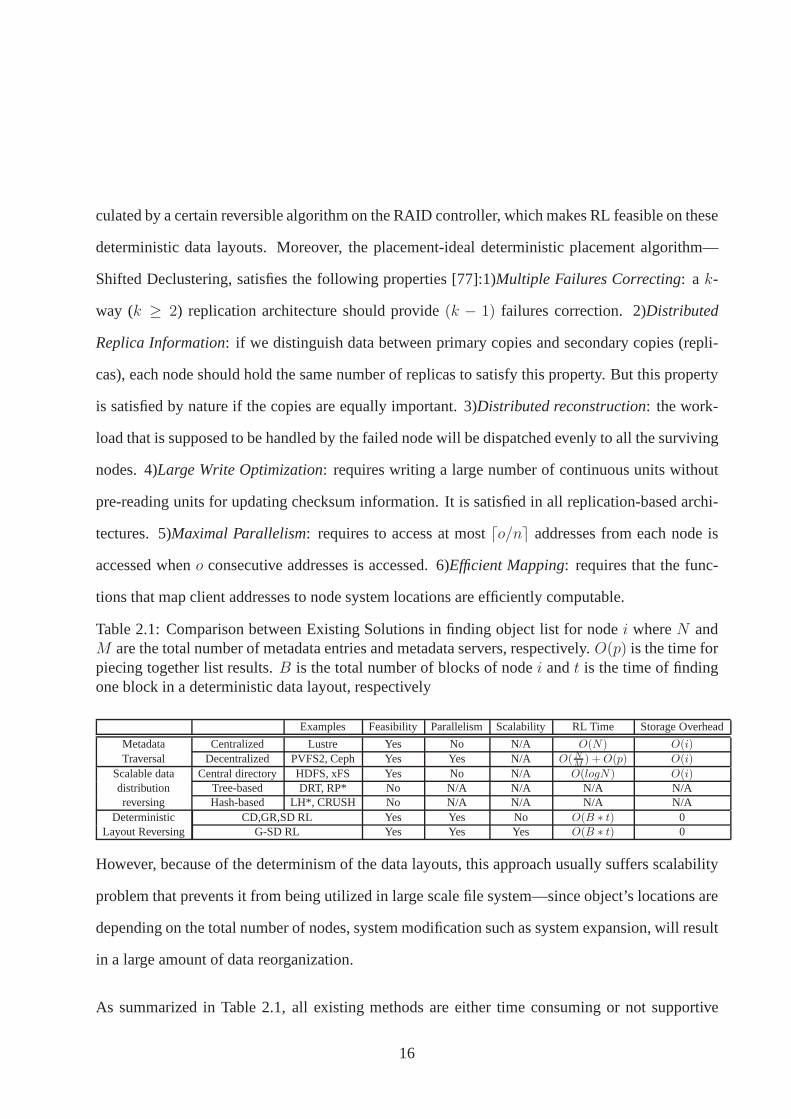
Table 2.1: Comparison between Existing Solutions in findingobject list for nodei whereN andM are the total number of metadata entries and metadata servers, respectively.O(p) is the time forpiecing together list results.B is the total number of blocks of nodei andt is the time of findingone block in a deterministic data layout, respectively
Examples Feasibility Parallelism Scalability RL Time Storage Overhead
Metadata Centralized Lustre Yes No N/A O(N) O(i)
Traversal Decentralized PVFS2, Ceph Yes Yes N/A O(NM ) +O(p) O(i)
Scalable data Central directory HDFS, xFS Yes No N/A O(logN) O(i)distribution Tree-based DRT, RP* No N/A N/A N/A N/Areversing Hash-based LH*, CRUSH No N/A N/A N/A N/A
Deterministic CD,GR,SD RL Yes Yes No O(B ∗ t) 0Layout Reversing G-SD RL Yes Yes Yes O(B ∗ t) 0
However, because of the determinism of the data layouts, this approach usually suffers scalability
problem that prevents it from being utilized in large scale file system—since object’s locations are
depending on the total number of nodes, system modification such as system expansion, will result
in a large amount of data reorganization.
As summarized in Table 2.1, all existing methods are either time consuming or not supportive
16
enough for the reverse lookup problem. Our previous work SD layout, as one type of deterministic
data layout, can achieve fast reverse lookup problem but it is not suitable for applying into the large-
scale system due to the scalability issue aforementioned. In this paper, we propose Group-based
Shifted Declustering (G-SD) data layout, to efficiently place objects and replications and solve the
flexibility and scalability of SD. It obeys all six properties meanwhile supports the reverse lookup
process within a relatively small overhead.
2.2 Power Efficiency and Reliability in Storage Systems
Based on our investigation and to the best of our knowledge, balancing among these three key
characteristics in degradation mode is not well studied. Partially because it is too complicated—on
one hand, performance and energy can be measured in fixed numbers and optimized according
to them. On the other hand, reliability in a storage system has been long time measured by Mean
Time to Data Loss (MTTDL), which is a probabilistic metric that is affected by various factors such
as disk temperature, utilization, wear-and-tear and etc. [67]. Previous researchers model reliability
by computing MTTDL based on continuous-time Markov Chain [69], which is complicated when
optimizing with performance and energy. This paper will focus on one specific factor in reliability
“recovery speed” as a measurement and provide a first step tryout in balancing energy, performance
and reliability. In this section, we summarize a thorough background and present key observations
that motivates our research.
2.2.1 Energyvs. Reliability
Taoet. al.studied the relationships between energy and reliability for independent disks [67]. They
built an empirical model called “PRESS” fed by three energy-saving-related reliability affected
17
factors: temperature, disk utilization, and disk speed transition frequency. As energy efficient
solutions skew data or requests into a subset of disks, the three factors are affected and thus the
reliability is influenced. For example, temperature for a skewed alive disk will become higher
and annual failure rate will increase. After evaluating each reliability factors, a general estimation
of reliability for the whole storage system will be generated by combining these factors together.
PRESS is able to help the following researchers to understand the reliability for each disks under
energy saving mode. Note that the reliability is measured inannual failure rate, a probabilistic
number. Our model, on the other hand, is looking at a different angle—the specific recovery
process.
2.2.2 Reliabilityvs. Performance
Suzhenet. al.discovered the relationship between reliability and performance in terms of node re-
construction speed and normal user requests for RAID systems [66]. As presented in the paper, the
reconstruction process has a mutually adversary impact on user I/O requests because they are com-
peting for I/O bandwidth. In order to avoid the performance degradation in node reconstruction,
they explored the data locality to determine the popular requests and redirect these requests into
surrogate RAID groups. In this work, energy is not included as only reliability and performance
are considered.
2.2.3 Energyvs. Performance
The trade-off energy versus performance has been studied for decades and extensive research has
been conducted. Before any formal metrics are defined for energy efficiency solutions, the key
idea is to putas many disks into low-power mode as possiblewithin the acceptable performance
tradeoff. Given a large cluster of disks, only a portion of them are accessed at any time so that the
18
rest can potentially be switched to the low-power mode. We summarized current solutions into the
following categories.
Hardware-based solutions adjust hardware configurations to achieve power savings.e.g. Guru-
murthi et al. introduced Dynamic Rotations Per Minute (DRPM) [28], attempting to save energy
by dynamically adjusting the disks’ speed. However, the feasibility of this solution is questionable
because it has not been widely adopted by the industry.
Software-based approaches use software schemes to conserve energy consumption of the storage
systems. The key problem is to seek solutions for extending the idle time so that a subset of
the storage system has enough time to switch the disks into low power mode. According to its
scheduling granularity, there are two major categories of the software-based solutions: 1)Storage-
level consolidationconcentrates thedatainto part of the disks so that others have no/little workload
and can be spun down. For example, Popularity Data Concentation (PDC) [46], skews the popular
data into a few number of disks so that the others can be switched to a low power mode. Similar
to MAID [23], PDC introduced a large amount of data movement overhead into the system. 2)
Request-level consolidationis currently used in replication-based systems. Instead ofskewing the
datainto part of the storage, it manipulatesrequestsand redirects them to replicas on active servers
when the others are in the low power mode. Representatives include EERAID [37] for RAID1
and RAID5 storage systems and Diverted Access [47] for replication-based storage systems.
Most recently, a specific metric named “energy proportional” is proposed by paper [17] to formally
define the relationships between energy and performance in acomputer system. They developed
this idea after identifying an unpleasant fact that currentservers will still consume more than 50
percent of the power even with no work conducted. The core principle is that system components
such as CPU, storage or router should consume an amount of energy compatible to the ratio of the
workload. Mathematically,wh
eh= wc
ec, wherewh andwc are the heaviest workload and the current
19
workload; andeh andec are the energy consumption under the heaviest workload and the current
energy consumption, respectively. It is soon widely accepted by both industry engineers and aca-
demic researchers as a designing guideline.e.g. PARAID [59] introduced power proportionality
into a RAID storage, using gear-based scheme to manage the active disks based on different power
settings in a RAID system. Amuret al. proposed “Rabbit” [15], a data layout for cluster-based
storage that can achieve read power proportionality and near power proportionality when node
failure happens. Thereskaet al. presented a power proportional layout “Sierra” [56] for cluster
storage that support not only read proportionality, but also write proportionality with the use of
Distributed Virtual Log (DVL). DVL absorbed updates to replicas that are on powered-down or
failed servers.
Although all current power proportion research considers fault-tolerant, only a part of the three
characteristics are taken into account in their design. Forinstance, Rabbit attempts to achieve
near power proportionality in degraded mode, which still focuses on saving energy after failure
happens. While Sierra aims to increase the recovery (rebuild) parallelism, which ignores energy
consumption in degradation mode. Furthermore, no proofs are provided why their solution can
achieve optimal tradeoffs under degraded mode. As recoverycompeting for I/O bandwidth with
normal performance and requiring specific nodes to open, thescenario is different with only con-
sidering power and performance. These three characteristics are mutually affected by each other.
This motivates us to conduct a theoretical study to explore their relationships by formulating a
multi-constraint problem “PERP”, which takes performanceand recovery requirements as con-
straints and power consumption as optimization object. It dynamically provisions the alive nodes
number and recovery speed at each time frame.
20
2.3 Block Management Schemes in Current DiFS
In this section, we examine the two possible solutions to reduce the BM costs for the master nodes,
including directory-based mapping and computation-basedmapping.
2.3.1 Directory-based Mapping
As mentioned above, current DiFSs distribute the blocks pseudo-randomly with the consideration
of network topology and rack-awareness and then store the locations of all blocks in a lookup
table/tree. As the block distributed by pseudo-random placement is correlation-free, this directory-
based mapping can easily scale-out with little reorganization overhead.
However, this approach incurs high cost on memory space and maintenance cost to keep the
directory-based mapping. 1) It consumes a large memory heapof the master nodes. As each
block has multiple replications, the size of this block map grows much faster than the size of the
file/block inodes. 2) Extra cares are needed to be taken to maintain the consistency between the
block map and the actual status of the data nodes and blocks. This includes block reports and
replication monitor/queue, where the block reports is usedfor the sanity check caused by software
bugs or unauthorized access; and replication motnitor/queue tracks the actual replica numbers of
each block to prevent losing data from hardware/software failures. These services also consumes
a large number of resources on the master node. For example, block reports, replication queue and
namespace management shares the same coarse-grain locks, which slows down the master server’s
performance.
To reduce the memory and maintenance cost in current DiFS, D.Sharpet. al. proposed a stan-
dalone block management in HDFS, which aims to separate the block management out of the
namenode [13]. As the namenode in the approach is solely handling the namespace operations,
21

this approach will improve the performance of the namenode and further improve the cluster’s
scalability. However, a slow metadata lookup may be resulted. Because compared with the origi-
nal lookup process that finishes within the namenode memory,each metadata lookup involves an
extra round of network messaging between namenodes and block manager nodes.
Evaluation of Existing Methods We briefly examine existing approaches used for block-to-node
mapping information management. As discussed in the first section, the major drawback of random
block placement methods [49, 18] and standone method [13] isthe large memory space overhead
for storing block-to-node information. In comparison, computational-based methods such as Hash-
ing or Crush [26, 62] could reduce the memory space overhead but fail to maintain block-to-node
information efficiently. Methods such as declustering [30,21] could reduce the memory space
overhead and support consistency checking efficiently. However, declustering techniques can’t be
directly applied to large-scale systems since they are not able to efficiently scale out during system
changes. We summarize how these methods satisfy the properties listed above in Table 2.2.
Table 2.2: Comparison among block-to-node mapping schemes, whereN is the number of datanodes,B is the number of blocks,c is the size of each block, andnet means one round of network
Examples Memory space Maintenance cost Efficient addressing Scale-out Recoverability
Directory DiFS default GFS,HDFS O(B*c) High O(1)∼O(B) Y HighStandalone Standalone O(B*c) Low O(1)∼O(B) Y High
based BM BM +O(net)Computation Hashing Ceph CRUSH O(CM) High O(log N) Y High
Declustering SD, Chain 0 Low O(1) N Lowbased Deister Deister O(NM) Low O(1) Y High
2.3.2 Computational-based Mapping
A more reasonable solution for reducing the block management costs is to use computational-based
mapping, which uses a deterministic addressing function for both block distributing and locating.
Representatives include hashing and declustering.
22

2.3.2.1 Hashing
Hashing is widely adopted by many distributed file systems, such as Amazon Dynamo [26],
OceanStore [35], Ceph [60] etc.. It allows the elimination of the cost for directory-based mapping
and the system can be balanced due to the random nature of hashfunctions. Based on the scope of
hash mapping, we divide the hash mapping methods into two categories: fully decentralized and
partially decentralized.
Fully decentralizedhashing distributes both namespace information (file inodes etc.) and blocks
on all servers. For example, peer-to-peer system such as OceanStore [35], CFS [25] maintain a
distributed hash table (DHT) as the distribution method. Itfirst hashes the directory/file names to
generate a key and distribute them across an unified key spaceacross the cluster. To achieve scale-
out ability, linear hashing [40], extensible hashing [27] and consistent hashing [33] are proposed.
Among them, systems such as Amazon Dynamo [26] and GlusterFS[3] adopt consistent hashing.
While LH∗ [41, 39] uses linear hashing. However, it is hard to apply fully decentralized in DiFS
because the architecture is fundamentally different. While DiFS uses a master-slave model, in
which a few master servers manage and guarantee strong consistency, block replications etc., the
fully hashing scheme is a peer-to-peer model and eventual consistency [26].
Partially decentralizeduses hash mapping to only distribute blocks across datanodes, while the
namespace is maintained by other methods such as tree/tablemapping. For example, Ceph main-
tains its namespace on a few metadata servers using sub-treepartitioning; and distribute the blocks
using CRUSH [29], a decentralized data distribution algorithm. CRUSH is built upon a data struc-
ture called cluster map which keeps track of the hardware infrastructure and failure domains. Both
distribution and data lookup process uses CRUSH algorithm so no location information is needed
to be stored. As the blocks are distributed deterministically, finding each block can be achieved via
calculation on any data nodes. While CRUSH provides similaradvantages as Deister, namely fast
23
deterministic mapping and little storage cost on metadata servers, its essential distribution hash
function is not reversible. As CRUSH does not have a centralized point of block management, the
consistency of a block is maintained by “peering”, which exchanging block reports within the same
placement group. This process involves a considerable amount of network messaging. While the
consistency check of Deister can be achieved gracefully by using a reversible addressing function
with little computation overhead.
2.3.2.2 Deterministic Declustering
The deterministic declustering, such as Chain-declustering [30], group-rotational declustering [21]
etc., is widely adopted in small-sized structures such as RAID systems. Different from hashing,
the object placement is pre-determined and calculated by a certain reversiblemath function on
the RAID controller. Using these approaches, all the block locations can be fast and easily calcu-
lated and no mapping information needs to be maintained. Moreover, the maintenance cost can
be significantly reduced by offloading the internal workloadto each datanode, reversing math dis-
tribution function, a large portion of the internal workload such as block report processing can be
offloaded to each datanode.
However, the declustering mapping cannot scale-out because the location of each block is cal-
culated based on the total number of nodes in the system, any changes such as node addition or
removal will result in large amount of data reshuffle. Also this layout is design for homogenous
environment where all nodes are identical. Moreover, declustering placement is designed for node
reconstruction, which takes far longer time than the DiFS re-replication time.
24
CHAPTER 3: GROUP-BASED SHIFTED DECLUSTERING
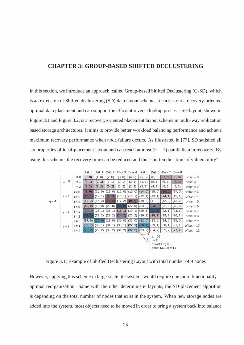
In this section, we introduce an approach, called Group-based Shifted Declustering (G-SD), which
is an extension of Shifted declustering (SD) data layout scheme. It carries out a recovery-oriented
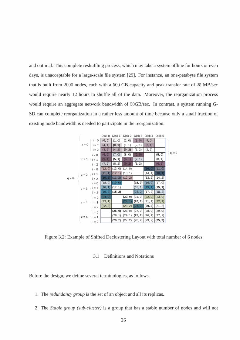
optimal data placement and can support the efficient reverselookup process. SD layout, shown in
Figure 3.1 and Figure 3.2, is a recovery-oriented placementlayout scheme in multi-way replication
based storage architectures. It aims to provide better workload balancing performance and achieve
maximum recovery performance when node failure occurs. As illustrated in [77], SD satisfied all
six properties of ideal-placement layout and can reach at most (n− 1) parallelism in recovery. By
using this scheme, the recovery time can be reduced and thus shorten the “time of vulnerability”.
(0, 0) (1, 0) (2, 0) (3, 0) (4, 0) (5, 0) (6, 0) (7, 0) (8, 0)
(8, 1) (0, 1) (1, 1) (2, 1) (3, 1) (4, 1) (5, 1) (6, 1) (7, 1)
(7, 2) (8, 2) (0, 2) (1, 2) (2, 2) (3, 2) (4, 2) (5, 2) (6, 2)
(9, 0) (10, 0) (11, 0) (12, 0) (13, 0) (14, 0) (15, 0) (16, 0) (17, 0)
(16, 1) (17, 1) (9, 1) (10, 1) (11, 1) (12, 1) (13, 1) (14, 1) (15, 1)
(14, 2) (15, 2) (16, 2) (17, 2) (9, 2) (10, 2) (11, 2) (12, 2) (13, 2)
(18, 0) (19, 0) (20, 0) (21, 0) (22, 0) (23, 0) (24, 0) (25, 0) (26, 0)
(24, 1) (25, 1) (26, 1) (18, 1) (19, 1) (20, 1) (21, 1) (22, 1) (23, 1)
(21, 2) (22, 2) (23, 2) (24, 2) (25, 2) (26, 2) (18, 2) (19, 2) (20, 2)
(27, 0) (28, 0) (29, 0) (30, 0) (31, 0) (32, 0) (33, 0) (34, 0) (35, 0)
(32, 1) (33, 1) (34, 1) (35, 1) (27, 1) (28, 1) (29, 1) (30, 1) (31, 1)
(28, 2) (29, 2) (30, 2) (31, 2) (32, 2) (33, 2) (34, 2) (35, 2) (27, 2)
Disk 0 Disk 1 Disk 2 Disk 3 Disk 4 Disk 5 Disk 6 Disk 7 Disk 8
z = 0
q = 4
z = 1
i = 0
i = 1
i = 2
i = 0
i = 1
i = 2
i = 0
i = 1
i = 2
i = 0
i = 1
i = 2
z = 2
z = 3
a = 33 i = 2 disk(33, 2) = 5 offset (33, 2) = 11
offset = 0
offset = 1
offset = 2
offset = 3
offset = 4
offset = 5
offset = 6
offset = 7
offset = 8
offset = 9
offset = 10
offset = 11
Figure 3.1: Example of Shifted Declustering Layout with total number of 9 nodes
However, applying this scheme in large-scale file systems would require one more functionality—
optimal reorganization. Same with the other deterministiclayouts, the SD placement algorithm
is depending on the total number of nodes that exist in the system. When new storage nodes are
added into the system, most objects need to be moved in order to bring a system back into balance
25
and optimal. This complete reshuffling process, which may take a system offline for hours or even
days, is unacceptable for a large-scale file system [29]. Forinstance, an one-petabyte file system
that is built from2000 nodes, each with a500 GB capacity and peak transfer rate of25 MB/sec
would require nearly12 hours to shuffle all of the data. Moreover, the reorganization process
would require an aggregate network bandwidth of50GB/sec. In contrast, a system running G-
SD can complete reorganization in a rather less amount of time because only a small fraction of
existing node bandwidth is needed to participate in the reorganization.
(0, 0) (1, 0) (2, 0) (3, 0) (4, 0)
(4, 1) (0, 1) (1, 1) (2, 1) (3, 1)
(3, 2) (4, 2) (0, 2) (1, 2) (2, 2)
(6, 0) (7, 0) (8, 0) (9, 0) (5, 0)
(9, 1) (5, 1) (6, 1) (7, 1) (8, 1)
(7, 2) (8, 2) (9, 2) (5, 2) (6, 2)
(12, 0) (13, 0) (14, 0) (10, 0) (11, 0)
(11, 1) (12, 1) (13, 1) (14, 1) (10, 1)
(10, 2) (11, 2) (12, 2) (13, 2) (14, 2)
(18, 0) (19, 0) (15, 0) (16, 0) (17, 0)
(16, 1) (17, 1) (18, 1) (19, 1) (15, 1)
(19, 2) (15, 2) (16, 2) (17, 2) (18, 2)
(24, 0) (20, 0) (21, 0) (22, 0) (23, 0)
(23, 1) (24, 1) (20, 1) (21, 1) (22, 1)
(22, 2) (23, 2) (24, 2) (20, 2) (21, 2)
(25, 0) (26, 0) (27, 0) (28, 0) (29, 0)
(28, 1) (29, 1) (25, 1) (26, 1) (27, 1)
(26, 2) (27, 2) (28, 2) (29, 2) (25, 2)
Disk 0 Disk 1 Disk 2 Disk 3 Disk 4 Disk 5
z = 0
q = 6
z = 1
i = 0
i = 1
i = 2
i = 0
i = 1
i = 2
i = 0
i = 1
i = 2
i = 0
i = 1
i = 2
i = 0
i = 1
i = 2
i = 0
i = 1
i = 2
z = 2
z = 3
z = 5
z = 4
q' = 2
Figure 3.2: Example of Shifted Declustering Layout with total number of 6 nodes
3.1 Definitions and Notations
Before the design, we define several terminologies, as follows.
1. Theredundancy groupis the set of an object and all its replicas.
2. TheStable group (sub-cluster)is a group that has a stable number of nodes and will not
26

influenced by the system expansion.
3. Theunstable group (sub-cluster)is a group that does not have a stable number of nodes and
will be influenced by the system expansion.
4. Thegroup reorganizationis the process of moving objects to other storage nodes in order to
keep the original layout after new storage nodes are added into the group.
Table 3.1: Summary of Notation
Symbols Descriptionsm Total number of nodes in the clustern Number of stable nodes in each sub-clustern′ Number of Unstable nodes in each sub-clusterk Number of units per redundancy groupa The address to denote a redundancy group(a, i) Thei-th unit in redundancy groupaq Number of iterations of a complete round
of layouty, z Intermediate auxiliary parametersnode(a, i) The node where the unit(a, i) is distributedoffset(a, i) The offset withinnode(a, i) where the unit
(a, i) is distributed
There are four system configuration parameters for the G-SD layout: the total number of nodes in
the systemm (m ≥ 2), number of nodes in a stable sub-clustern (n ≤ m), number of nodes in an
unstable sub-clustern′ (n′ ≤ n+ k+1) and the number of units per redundancy groupk (k ≤ m).
Within a redundancy group, the units are named from 0 tok−1, and we view the unit 0 as the object
(primary copy), and other units as replica units (secondarycopies). Distinguishing objects from
their replica is only for the ease of representation, although they are identical. We use an address
a (a ≥ 0) to denote a redundancy group, anda can also be considered as a redundancy group ID.
Each unit is identified by the name(a, i), wherea is the redundancy group ID, and0 ≤ i ≤ k − 1.
Without the loss of generality,(a, 0) represents the object, and(a, i) with i > 0 represents thei-th
replica unit. The location of the unit(a, i) is represented by a tuple(node(a, i), offset(a, i)). A
complete round of layout is obtained byq iterations, and in each iteration, one row of data units and
27

k− 1 rows of replica units are placed, so that the total rows of units in a complete round isr = kq.
Repeating complete rounds of layouts also yields placement-ideal layouts. In the following, we
only consider the layouts within a complete round.
3.2 Group-based Shifted declustering Scheme
The G-SD is proposed to minimize the reorganization overhead of shifted declustering layout so
that this layout can be utilized in large-scale file systems.It is based upon a simple principle:
storage nodes or nodes are divided into groups (sub-clusters) so that when nodes are being added
or removed, the reorganization process would only influencethe nodes within one group rather
than the whole file system, as traditional shifted declustering does.
In G-SD, suppose we havem nodes in the system and we divide them into multiple stable groups
with each group containingn nodes and one unstable group withn′ (n′ ≤ n + k + 1) nodes.
In each group, a shifted declustering scheme is applied to optimize the replica placement so that
maximum recovery performance can be achieved when node failure occurs. That is, if nodej in
groupa failed, the number of nodes that could participate in the recovery is maximized within the
group. While members in one group are correlated with each other, groups are independent— each
holding disjoint fractions of objects for the whole system.Replicas will not be placed among dif-
ferent group members. By keeping little relationships between different groups, the reorganization
process brought by node addition will only influence the members within one group, leaving other
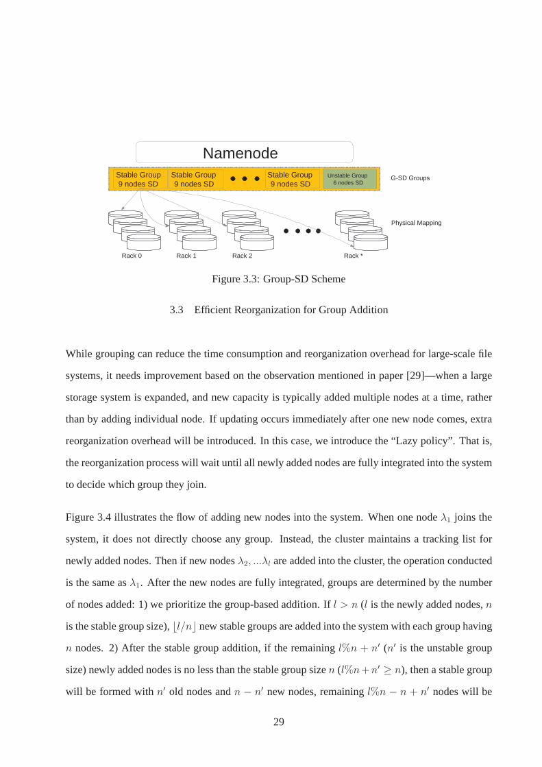
groups unaffected. Figure 3.3 shows an example of G-SD scheme: nodes are divided into differ-
ent sub-clusters. Sub-cluster 1, 2, and 3 all consist of 9 nodes, which is the stable group number,
while sub-cluster 4 is unstable group with 6 nodes. Each sub-cluster is managed by local shifted
declustering layout—1, 2, 3 are shown as Figure 3.2, 4 is shown as Figure 3.1, respectively.
28
Namenode G-SD Groups
Physical Mapping
Stable Group 9 nodes SD
Stable Group 9 nodes SD
Stable Group 9 nodes SD
Unstable Group 6 nodes SD
Rack 0 Rack 1 Rack 2 Rack *
Figure 3.3: Group-SD Scheme
3.3 Efficient Reorganization for Group Addition
While grouping can reduce the time consumption and reorganization overhead for large-scale file
systems, it needs improvement based on the observation mentioned in paper [29]—when a large
storage system is expanded, and new capacity is typically added multiple nodes at a time, rather
than by adding individual node. If updating occurs immediately after one new node comes, extra
reorganization overhead will be introduced. In this case, we introduce the “Lazy policy”. That is,
the reorganization process will wait until all newly added nodes are fully integrated into the system
to decide which group they join.
Figure 3.4 illustrates the flow of adding new nodes into the system. When one nodeλ1 joins the
system, it does not directly choose any group. Instead, the cluster maintains a tracking list for
newly added nodes. Then if new nodesλ2, ...λl are added into the cluster, the operation conducted
is the same asλ1. After the new nodes are fully integrated, groups are determined by the number
of nodes added: 1) we prioritize the group-based addition. If l > n (l is the newly added nodes,n
is the stable group size),⌊l/n⌋ new stable groups are added into the system with each group having
n nodes. 2) After the stable group addition, if the remainingl%n + n′ (n′ is the unstable group
size) newly added nodes is no less than the stable group sizen (l%n+n′ ≥ n), then a stable group
will be formed withn′ old nodes andn − n′ new nodes, remainingl%n − n + n′ nodes will be
29

formed as an unstable group. Ifl%n + n′ < n, thel%n newly added nodes will join the unstable
group.
For instance, in a three-way replication system the optimalsub-cluster sizen (Section 3.6) is 10
and there are 27 nodes already in the system, which are subsequently divided into three groups
(2*10 nodes stable groups,7 nodes unstable group). If adding 23 new nodes into the cluster, the
newly added group will be divided into two stable groups first, which contains 10 nodes each. The
remaining 3 nodes will join the existing unstable group to produce a 10 nodes stable group. If 27
nodes are added into the cluster, the remaining 7 nodes will be divided into two parts, first, three
nodes will participate in the former unstable group to form a10 nodes stable group. The left 4
nodes will form an unstable group due to the minimum node number local shifted declustering
layout requiring for three-way replication isn ≥ 4 for each group. Since node addition only
maintains the information about the number of newly added nodes and this process takes little
space, the total storage requirement of tracking this list could be negligible. By using the “lazy
policy”, tracking list and group “prior” methods, we are able to reduce the reorganization overhead
by merging several reorganization process into one or even totally eliminating the reorganization
process in some cases (will mention in Section 3.4).
We consider node retirement to be the same as node recovery because the retiring node has to
“shed” its data to other data nodes which will result in a temporary local shifted declustering un-
balance. Though node departure could be supported by our solution, it costs extra overhead is
needed to reorganize the replicas in an already balanced shifted declustering layout sub-cluster.
Since in our solution, recovery is parallelized and efficient, we believe that substituting the retired
node and transferring all the data to the new node is a better idea than nodes departure and rebal-
ancing of loads. Before substitution, if some nodes are not available, the workload could still be
evenly distributed into the existing nodes, which will not degrade the performance substantially.
30
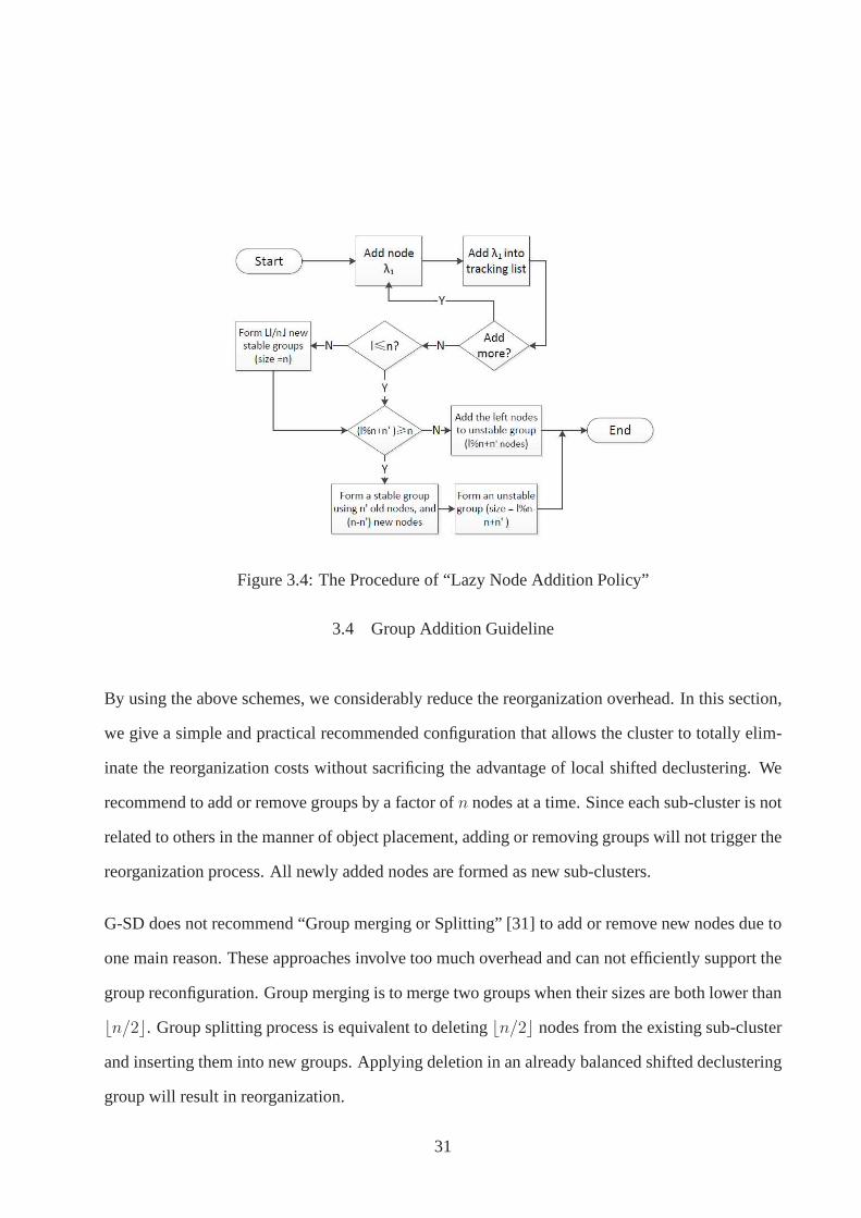
Figure 3.4: The Procedure of “Lazy Node Addition Policy”
3.4 Group Addition Guideline
By using the above schemes, we considerably reduce the reorganization overhead. In this section,
we give a simple and practical recommended configuration that allows the cluster to totally elim-
inate the reorganization costs without sacrificing the advantage of local shifted declustering. We
recommend to add or remove groups by a factor ofn nodes at a time. Since each sub-cluster is not
related to others in the manner of object placement, adding or removing groups will not trigger the
reorganization process. All newly added nodes are formed asnew sub-clusters.
G-SD does not recommend “Group merging or Splitting” [31] toadd or remove new nodes due to
one main reason. These approaches involve too much overheadand can not efficiently support the
group reconfiguration. Group merging is to merge two groups when their sizes are both lower than
⌊n/2⌋. Group splitting process is equivalent to deleting⌊n/2⌋ nodes from the existing sub-cluster
and inserting them into new groups. Applying deletion in an already balanced shifted declustering
group will result in reorganization.
31
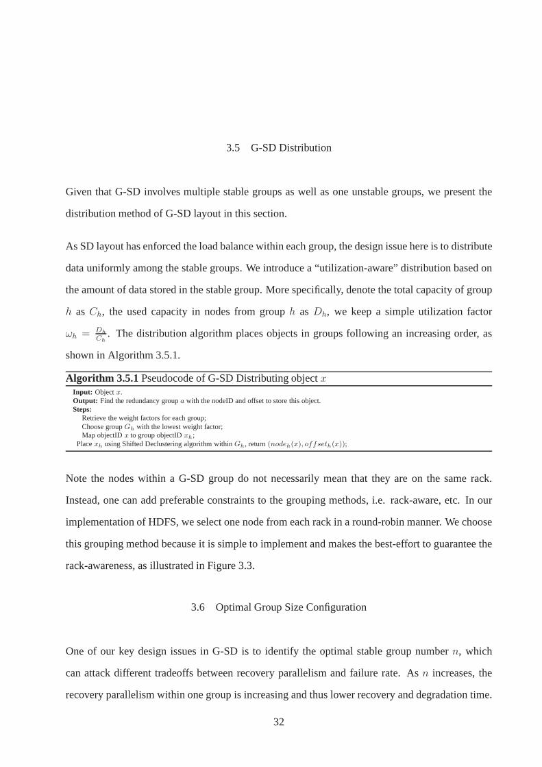
3.5 G-SD Distribution
Given that G-SD involves multiple stable groups as well as one unstable groups, we present the
distribution method of G-SD layout in this section.
As SD layout has enforced the load balance within each group,the design issue here is to distribute
data uniformly among the stable groups. We introduce a “utilization-aware” distribution based on
the amount of data stored in the stable group. More specifically, denote the total capacity of group
h asCh, the used capacity in nodes from grouph asDh, we keep a simple utilization factor
ωh = Dh
Ch. The distribution algorithm places objects in groups following an increasing order, as
shown in Algorithm 3.5.1.
Algorithm 3.5.1 Pseudocode of G-SD Distributing objectxInput: Objectx.Output: Find the redundancy groupa with the nodeID and offset to store this object.Steps:
Retrieve the weight factors for each group;Choose groupGh with the lowest weight factor;Map objectIDx to group objectIDxh;
Placexh using Shifted Declustering algorithm withinGh, return(nodeh(x), offseth(x));
Note the nodes within a G-SD group do not necessarily mean that they are on the same rack.
Instead, one can add preferable constraints to the groupingmethods, i.e. rack-aware, etc. In our
implementation of HDFS, we select one node from each rack in around-robin manner. We choose
this grouping method because it is simple to implement and makes the best-effort to guarantee the
rack-awareness, as illustrated in Figure 3.3.
3.6 Optimal Group Size Configuration
One of our key design issues in G-SD is to identify the optimalstable group numbern, which
can attack different tradeoffs between recovery parallelism and failure rate. Asn increases, the
recovery parallelism within one group is increasing and thus lower recovery and degradation time.
32
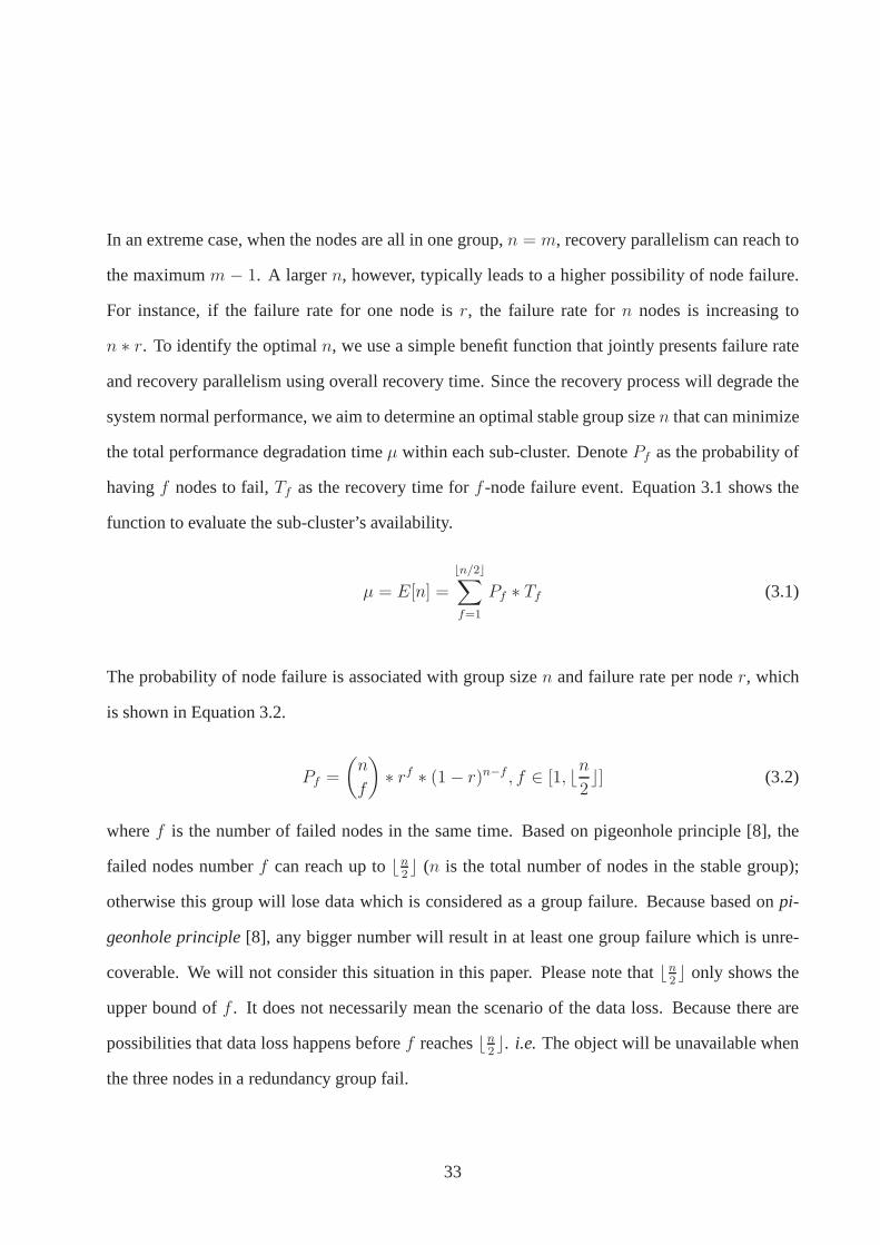
In an extreme case, when the nodes are all in one group,n = m, recovery parallelism can reach to
the maximumm − 1. A largern, however, typically leads to a higher possibility of node failure.
For instance, if the failure rate for one node isr, the failure rate forn nodes is increasing to
n ∗ r. To identify the optimaln, we use a simple benefit function that jointly presents failure rate
and recovery parallelism using overall recovery time. Since the recovery process will degrade the
system normal performance, we aim to determine an optimal stable group sizen that can minimize
the total performance degradation timeµ within each sub-cluster. DenotePf as the probability of
havingf nodes to fail,Tf as the recovery time forf -node failure event. Equation 3.1 shows the
function to evaluate the sub-cluster’s availability.
µ = E[n] =
⌊n/2⌋∑
f=1
Pf ∗ Tf (3.1)
The probability of node failure is associated with group sizen and failure rate per noder, which
is shown in Equation 3.2.
Pf =
(n
f
)∗ rf ∗ (1− r)n−f , f ∈ [1, ⌊n
2⌋] (3.2)
wheref is the number of failed nodes in the same time. Based on pigeonhole principle [8], the
failed nodes numberf can reach up to⌊n2⌋ (n is the total number of nodes in the stable group);
otherwise this group will lose data which is considered as a group failure. Because based onpi-
geonhole principle[8], any bigger number will result in at least one group failure which is unre-
coverable. We will not consider this situation in this paper. Please note that⌊n2⌋ only shows the
upper bound off . It does not necessarily mean the scenario of the data loss. Because there are
possibilities that data loss happens beforef reaches⌊n2⌋. i.e. The object will be unavailable when
the three nodes in a redundancy group fail.
33

The recovery time is influenced by the recovery parallelism.As objects are evenly distributed in
one group using local shifted declustering layout. All other nodes in the same group will partic-
ipate in the recovery in a parallel manner. Assumet is the time for recovering one failed node
sequentially, the parallel recovery (see Section 3.8.2 fordetail) time is represented in Equation 3.3.
Tf =t ∗ fn− f
, 1 ≤ f ≤ ⌊n2⌋ (3.3)
So the optimal value of stable group sizen is the one that could minimize theµ in Equation 3.1, as
shown follows.
µ =
⌊n/2⌋∑
f=1
Pf ∗ Tf (3.4)
=
⌊n/2⌋∑
f=1
(n
f
)∗ rf ∗ (1− r)n−f ∗ tf
n− f
=
(n
1
)r(1− r)n−1 t
n− 1+
(n
2
)r2(1− r)n−2
∗ 2t
n− 2+
(n
3
)r3(1− r)n−3 3t
n− 3+ ...+
(n
⌊n2⌋
)
∗r⌊n2⌋(1− r)n−⌊n
2⌋ ⌊n
2⌋t
n− ⌊n2⌋
where we ignore the cases that nodes fail in the middle of a recovery process.
As t and r are all constant, to minimizeµ we calculate the derivative (µ′) and letµ′ = 0 to
retrieve the extrema. For example, we chooser = 3% per year. According to Schroederet al.’s
observation [50], in a real-world large storage and computing systems, the ARR (annual replace
rate) of hard drives is between 0.5% and 13.8%, and 3% on average. The reasonable and optimal
n is 9 if n is odd and 8 ifn is even.
34
3.7 G-SD Reverse Lookup
In this section, we present the reverse lookup mechanism in our G-SD. When a node fails in
a cluster, reverse lookup in G-SD may involve two hierarchical levels: acquiring the group ID
in which the failed node exists, and retrieving the object list from the local shifted declustering
reverse function. This hierarchical design is to provide fast and guaranteed reverse lookup that will
find out the objects needed to be recovered in a fairly short time.
Each query is performed in the following sequences. First, one node failure is detected by heart-
beats, and it will return the tuple< groupID, nodeID >. Given this tuple and the upper bound of
the block ID within this group, the system could conduct the reverse lookup. Second, retrieve the
object list by using the shifted declustering reverse function. We would like to give an example for
three-way replication. The reverse lookup algorithm can beabstracted as: assumingk (the number
of units per redundancy group) andn (the number of nodes in the sub-cluster) are known system
parameters,d (node/node ID) ando (offset) are given location, find out the redundancy group IDa
located on noded and offseto.
In three-way replication withn = 4 or n is odd, the local reverse lookup function could be sum-
marized in through Equation 3.5 to Equation 3.9.
35
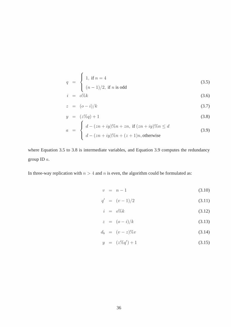
q =
1, if n = 4
(n− 1)/2, if n is odd(3.5)
i = o%k (3.6)
z = (o− i)/k (3.7)
y = (z%q) + 1 (3.8)
a =
d− (zn + iy)%n+ zn, if (zn + iy)%n ≤ d
d− (zn + iy)%n+ (z + 1)n, otherwise(3.9)
where Equation 3.5 to 3.8 is intermediate variables, and Equation 3.9 computes the redundancy
group IDa.
In three-way replication withn > 4 andn is even, the algorithm could be formulated as:
v = n− 1 (3.10)
q′ = (v − 1)/2 (3.11)
i = o%k (3.12)
z = (o− i)/k (3.13)
db = (v − z)%v (3.14)
y = (z%q′) + 1 (3.15)
36

if (node(a, 0) < db andnode(a, 0) + iy ≥ db)
ornode(a, 0) > db andnode(a, 0) + iy ≥ db + n′)
if (zn + iy + 1)%n ≤ d)
a = d− (zn + iy + 1)%v + zn
elsea = d− (zn + iy + 1)%n+ zn
else if((zn + iy)%n ≤ d)
a = d− (zn + iy)%n+ zn
elsea = d− (zn + iy + 1)%n+ (z + 1)n
wherea is different due to the fact that the placement fornode(a, i) varies before or after the
bubble that is mentioned in [77].
3.8 Analysis
In this section, we conduct a comprehensive analysis on two key goals of G-SD: reorganization
overhead and data availability.
3.8.1 Reorganization Overhead Analysis
G-SD aims to take the advantage of the fast and efficient reverse lookup of the shifted decluster-
ing algorithm and minimize its reorganization overhead. Here we explicitly give the overhead of
adding new nodes into a shifted declustering layout and compare it with a system using G-SD.
Assume that there is a shifted declustering layout withα nodes and we are about to addβ nodes
into this layout. The total number of objects that needs to bemoved from one node to another is as
37

follows.
R(α, β) =
[(q − 1)α+ (β + 1)]× 3, if βis even andαisodd
[(q − 1)α+ (β + 1)]× 3 + 2, if βis odd andαis even
[(q − 1)α]× 3, if β = 1andα is odd
[(q − 1)α+ β]× 3, if βis odd,α > 1andmis odd
[(q − 1)α+ β]× 3 + 2, if βis even, andαis even
(3.16)
In Equation 3.16,q = 1 if α is 4,q = (α− 1)/2 if α is odd, orq = (α− 2)/2 if v is even.R(α, β)
is mainly determined by the number of objects that need to be moved from one node to another.
The proof is provided in the Appendix. Suppose that the overhead of moving one object to another
node isv, the total reorganization overhead isv ∗ R(α, β). Then we compare the reorganization
overhead between SD and G-SD layout.
1. In a system with SD layout, the total number of nodes ism. Whenl nodes are added into
the system, the total overhead of balancing the shifted declustering layout is equalOSD =
v ∗R(m, l)
2. In G-SD with total ofm nodes, at most one unstable group is affected when adding nodes
into the system. Thus the reorganization overhead will be limited to the unstable group size
n′ < n + 4. Specifically, when addingl new nodes into this system, the total overhead is
shown as follows.
OGSD =
v ∗R(n′, n− n′), if l%n + n′ ≥ n + 4
v ∗R(n′, l%n), if l%n + n′ < n+ 4(3.17)
As shown in Figure 3.4, whenl%n + n′ ≥ n + 4, the reorganization overhead is generated
from forming one stable group usingn′original unstable group nodes and(n − n′) newly
38

added nodes. Whenl%n + n′ < n + 4, the overhead is generated from addingl%n new
nodes into the original unstable group (n′ nodes).
0 10 20 30 40 50 60 70 80 90 1000
2000
4000
6000
8000
10000
12000
14000
16000
18000
Group(Cluster) size for G−SD(SD)
Reo
rgan
izat
ion
over
head
(n
umbe
r of
reo
rgan
ized
obj
ects
)
G−SDSD:l=10SD:l=20SD:l=50SD:l=100SD:l=500
Figure 3.5: Reorganization overhead (number of objects reorganized) comparison in differentgroup size (n) and different number of nodes added (l)
Figure 3.5 presents the overhead comparisons of different group sizes and different numbers of
added nodes. In this figure, we assume thatv as 1. We can see from Figure 3.5, the reorganization
overhead is directly related to the number of nodes in the systemm and number of nodes added
l. Specifically, in a SD layout with the number of nodesm growing from 4 to 100, every line is
maintaining an increasing trend. Also, as the number of nodes added increases, the trend goes
sharper. On the other hand, reorganization overhead in a G-SD is in is fluctuating around a small
number and is not directly affected bym andl.
3.8.2 Analysis of Data Availability
With our mathematical proof, we have demonstrated that the reorganization overhead has been
bounded into a reasonable range and support fast reverse lookup to speed up the recovery process.
39
In this section, we study and analyze the impact of G-SD from adifferent angle ofdata availabil-
ity,which is the system’s ability of providing sufficient and correct data throughout failures. High
data availability means that data replicas should still be available when failure happens. More
specifically, in a multi-way replication systems, the system runtime can still provide services by
redirecting the requests to other replicas when node failure happens. We quantify this property as
P (l) which meansthe probability that the system does not lose data after thel-th node fail-
ure. Suppose the failure rate for each node isλ. Apparently,P (l) = 1 if l < k, andP (l) = 0 if
l > lmax, wherelmax is the possible maximum number of failed nodes without losing data. Withl
failed nodes, there arem− l nodes which may fail, so the rate of another node failure is(m− l)λ,
whereλ represents the node failure rate.
As the value ofP (l) and the recovery rateµl when the system hasl failed nodes are different
among different layouts. In the following two sub-sections, we will derive the values ofP (l) and
µ(l).
Group-based Shifted Declustering G-SD layout divides the whole cluster into small groups so
that the reorganization overhead can be reasonably boundedwhen system expands. The data will
be lost if the failed nodes are in the same group. More specifically, in one sub-cluster, data loss
will happen uponl node failures if there exists a set ofk failed nodes with a fixed distance between
neighboring nodes in a G-SD group.The value of P (l) (no data loss after l node failures)
is the probability that given l failed nodes, for anyk out of the l nodes, there is no fixed
distance between neighboring ones in a G-SD group.Therefore, we are looking for the subset
{i0, i1, . . . , il−1} ⊆ [0, . . . , n − 1] (n is the number of nodes in one stable group) such that
∀{j0, j1, . . . , jk−1} ⊆ {i0, i1, . . . , il−1}, where{j0, j1, . . . , jk−1} is a combination ofk
elements out of the subset{i0, i1, . . . , il−1}, and not existd for all m ∈ {0, 1, . . . , k − 1},
j(m+1) modk
= (jm + d) modn.
40

DenoteSgsd(m, k, l) as the number of choices to selectl nodes from ak-way replicated system with
m number of nodes; obeying the conditions shown above. Therefore,Pgsd(l) can be computed as
follows,
Pgsd(l) =
Sgsd(m, k, l)/C(m, l) if n is odd orn = 4
Sgsd(m′, k, l)/C(n, l) if n is even andn > 4
(3.18)
wherem′ is the maximum number that is smaller thanm+ and there exists a basic solution for
m′-node. In our case whenk = 3, m′ = m − 1. For both cases, ifl = k, Pgsd(k) =1−m(n+−1)]
2C(m,k),
because if the first failed node is chosen, there are(n− 1)/2 types of distances to decide the other
two failed nodes to cause data loss. There arem ways to select the first node, so there are in total
m(n− 1)/2 ways to selectk failed nodes to lose data.
Random Distribution Many current enterprise-scale storage systems adopt random data layout
schemes to distribute data units among storage nodes [49, 18, 60]. There is also theoretical re-
search on algorithms for random data distribution in large-scale storage systems [29]. Random
layout attracts people’s interests because it brings a statistically balanced distribution of data, thus
providing optimal parallelism and load balancing in both normal and degraded mode.
The probability of losing (or not losing) data uponl failed nodes depends not only onl, the total
number of nodes (m), and the number of replicas in each redundancy group (k), but also on the
number of redundancy groups (r). The number of redundancy groups is a function ofm, the used
capacity of nodes (S), and the size of a data unit (s). We assume that the used space of each node
is the same, and the size of a data unit is fixed. The number of redundancy groups can be derived
asr =S ×m
s× k, whereS × n means the total used space for data storage, ands × 3 is the space
used by one redundancy group.
There areC(m, k) ways to distribute a redundancy group. We assume that an ideal random declus-
41
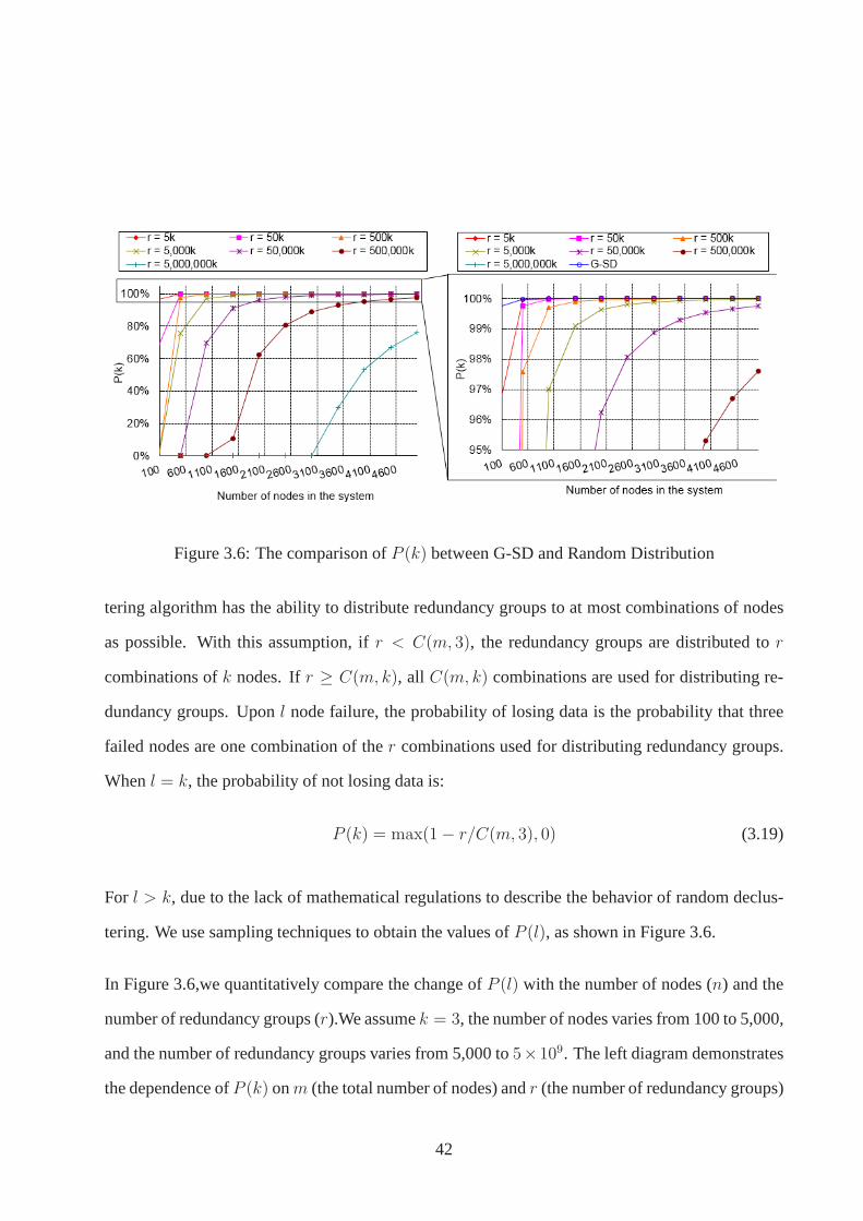
Figure 3.6: The comparison ofP (k) between G-SD and Random Distribution
tering algorithm has the ability to distribute redundancy groups to at most combinations of nodes
as possible. With this assumption, ifr < C(m, 3), the redundancy groups are distributed tor
combinations ofk nodes. Ifr ≥ C(m, k), all C(m, k) combinations are used for distributing re-
dundancy groups. Uponl node failure, the probability of losing data is the probability that three
failed nodes are one combination of ther combinations used for distributing redundancy groups.
Whenl = k, the probability of not losing data is:
P (k) = max(1− r/C(m, 3), 0) (3.19)
For l > k, due to the lack of mathematical regulations to describe thebehavior of random declus-
tering. We use sampling techniques to obtain the values ofP (l), as shown in Figure 3.6.
In Figure 3.6,we quantitatively compare the change ofP (l) with the number of nodes (n) and the
number of redundancy groups (r).We assumek = 3, the number of nodes varies from 100 to 5,000,
and the number of redundancy groups varies from 5,000 to5×109. The left diagram demonstrates
the dependence ofP (k) onm (the total number of nodes) andr (the number of redundancy groups)
42
in random declustering. Each line reflects the value change of P (k) for a certainr and a varying
m. We can see that with a fixed number of nodes, the more redundancy groups the system has, the
smaller isP (k), which means that it is easier for the system to lose data uponk node failures. A
recent work [16] shows similar results and developed CopySet based on this observation. In their
observation, a1% of node failure will definitely result in a data loss when the node size is larger
than300. We enlarge the portion nearP (k) = 1 to the right diagram, and add theP (k) values of
G-SD. In this configuration, the group size is set as9. We can see thatP (k) of G-SD is constantly
approaching 1.
3.9 Evaluation
G-SD is a scalable layout that supports fast and efficient reverse lookup. In this section, we describe
our implementation of G-SD on two distributed file systems Ceph and HDFS. We also provide the
results of our experiments on a large-scale cluster on G-SD’s impact on the systems’ performance
and reverse lookup latency.
We set up the experiment environment using Marmot cluster [7, 64], which is a cluster of PRObE [64]
on-site project and housed at CMU in Pittsburgh. The system itself consists of 128 nodes/256 cores
and each node has dual 1.6 GHz AMD Opteron processors, 16 GB memory, Gigabit Ethernet, and
local storage of 2TB Western Digital SATA HDD.
In the evaluations, we make comparisons of G-SD reverse lookup with two widely adopted reverse
lookup methods: metadata traversal methods and tree-reversing methods. Firstly. we conduct ex-
periments to compare G-SD RL with the decentralized metadata traversal method on Ceph release
0.87 [60]. Ceph is an ever-popular open-source distributed object storage system. It has evolved
from Sage Weilet. al.’s Ph.D dissertation in the University of California at Santa Cruz (UCSC).
Ceph distributes its data using CRUSH algorithm to avoid a single point of failure and the data is
43
replicated, making it fault tolerant. The experiments are run on36 nodes of the marmot cluster
with 4 metadata servers and32 Object Storage Daemons (OSDs).
Secondly, we perform two sets of experiments on HDFS2.2.0 using32 nodes of Marmot cluster.
HDFS is a distributed, scalable, and portable file-system written in Java for the Hadoop frame-
work [18]. It was originally developed by Yahoo! to facilitate its search-engine and now becomes
the foundation for the current big-data applications. Since HDFS support replication at the first
place. We first compare the performance of G-SD layout with the HDFS default rack-aware ran-
dom layout. Then series of experiments are conducted to compare the G-SD RL speed and HDFS
tree-reversing speed.
3.9.1 Implementation on Ceph
The implementation of G-SD on Ceph is mainly consist of two modules: 1) the G-SD distribution
algorithms modification on CRUSH module. More specifically,we still keep the CRUSH map run-
ning on each Ceph OSD but substitute thecrush do rule() (that outputs the result vector) method
in classCrushWrapper (which is the exposed class for CRUSH) to callGSD distribute() so
that it outputs the results of G-SD distribution. Before doing that, we need to make sure that the
objects are not stored in hash keys because G-SD uses sequential number to distribute the objects.
In order to do so, we implement a method in classhash to just output the input number as the object
ID. 2)GSD RL() is implemented as an independent function that is called in classOSDMonitor
after the OSD is proposed to be marked “down” and receives positive response from Paxos service.
The native metadata traversal method of Ceph is a complicated process. When a monitor receives
notifications saying that an OSD node timeout, it will mark the node as “down” in its master cluster
map (more specifically, OSDMap) and increase its version number. Then it will send the updated
cluster map back to the reporting OSDs and also a random OSD, which will conduct a sync with
44
their current OSDMap to recognize the PGs that have been impacted by the “down” node. When a
PG is recognized as the impacted group by this node failure, it will be marked as degraded and start
to pile up the PG logs for its later recovery process. Note each failed node has many PG residing on
it and each PG handles its objects independently, thus this RL process can be time efficient because
it is done in parallel with the number of PGs in the cluster. However, the updated OSDMap will
need some time to propagate within the cluster before all impacted PG are recognized and there
are also message exchanges between monitor nodes and the OSDs. Compared with this approach,
our implementation directly goes to theOSDMonitor and prepares the object lists on the failed
node for later recovery (if necessary).
3.9.2 Evaluation on Ceph
To evaluate the performance and metadata traversing speed on Ceph, we use Ceph’s embedded
benchmarking tool RADOS bench to ingest different sizes of data into Ceph cluster. RADOS
bench is a part of RADOS object storage utility and supports different IO modes such as write,
sequential read and random read. If not specified, the default object size is 4 MB, and the default
number of simulated threads (parallel writes) is 16. In all tests, the number of replications is set to
three. This set of experiments are run on36 nodes on Marmot cluster with four monitor nodes and
32 OSDs.
For the throughput test, we run the RAODS bench utility on both clusters and the results (MB/s)
are shown at the end of each run. For reverse lookup tests, we monitor the time after a node is
manually bring down using “ceph osd out osd-xx” command. This guarantees that an updated
OSD map will be sent out by the OSDMonitor and the recovery will be initiated. To monitor
the reverse lookup time, we insert a timer between the function On Ceph, we monitor the reverse
lookup time by set a timer for the function callgetlog.get missing() within OSD class, which
45
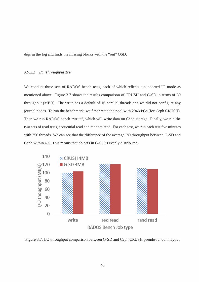
digs in the log and finds the missing blocks with the “out” OSD.
3.9.2.1 I/O Throughput Test
We conduct three sets of RADOS bench tests, each of which reflects a supported IO mode as
mentioned above. Figure 3.7 shows the results comparison ofCRUSH and G-SD in terms of IO
throughput (MB/s). The write has a default of 16 parallel threads and we did not configure any
journal nodes. To run the benchmark, we first create the pool with 2048 PGs (for Ceph CRUSH).
Then we run RADOS bench “write”, which will write data on Cephstorage. Finally, we run the
two sets of read tests, sequential read and random read. For each test, we run each test five minutes
with 256 threads. We can see that the difference of the average I/O throughput between G-SD and
Ceph within4%. This means that objects in G-SD is evenly distributed.
Figure 3.7: I/O throughput comparison between G-SD and CephCRUSH pseudo-random layout
46

3.9.2.2 Decentralized Metadata Traversingvs. G-SD Reverse Lookup
In this section, we compare the response latency of G-SD RL with the decentralized metadata
traversal scheme used by Ceph. We set the object sizes as256KB, 1MB, and4 MB; write a total
amount of data size as66 GB (total≈ 200 GB), 166 GB (total≈ 500 GB) and333 GB (total≈ 1
TB) and666GB (total≈ 2 TB) using RADOS bench. The number of PGs are2048.
Figure 3.8 presents a comparison of the average response latency between G-SD RL and Ceph
PG decentralized metadata traversing (DMT) in different configurations. Although both methods
can find the missing objects in seconds, the curves representing G-SD RL times are always at the
bottom of the diagram. So G-SD RL provides faster reverse lookup than Ceph PG DMT in our
setup. Overall the average speedup of G-SD RL is 6x faster. With the same setup, we expect
that Ceph DMT to complete faster if the number of OSDs increase while the number of PGs stays
the same. This is because the number of PGs located on each node is less, meaning DMT needs
to find fewer missing objects. However, as discussed above, Ceph recovery is not simple process
which involves in OSD map update, map prorogation, find incremental on primary and then get the
missing objects. This whole process can be long comparing with only G-SD RL directly finding
the missing object list.
3.9.3 Implementation on HDFS
We implement G-SD layout solely on the block management module of HDFS Namenode (meta-
data server). The implementation is relatively straightforward because HDFS has provided the
interface to support a configurable data placement policy inversion 2.2.0. G-SD forms its groups,
assigns G-SD group IDs and maintains a mapping from datanodeID to GSDdatanode ID (datan-
ode ID within a G-SD group). After all the nodes have been added into the cluster, the Namenode
47
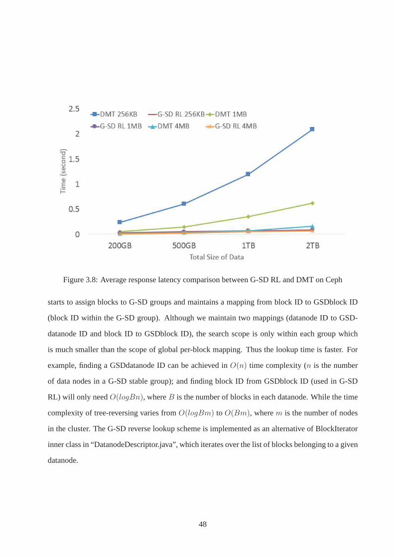
Figure 3.8: Average response latency comparison between G-SD RL and DMT on Ceph
starts to assign blocks to G-SD groups and maintains a mapping from block ID to GSDblock ID
(block ID within the G-SD group). Although we maintain two mappings (datanode ID to GSD-
datanode ID and block ID to GSDblock ID), the search scope is only within each group which
is much smaller than the scope of global per-block mapping. Thus the lookup time is faster. For
example, finding a GSDdatanode ID can be achieved inO(n) time complexity (n is the number
of data nodes in a G-SD stable group); and finding block ID fromGSDblock ID (used in G-SD
RL) will only needO(logBn), whereB is the number of blocks in each datanode. While the time
complexity of tree-reversing varies fromO(logBm) to O(Bm), wherem is the number of nodes
in the cluster. The G-SD reverse lookup scheme is implemented as an alternative of BlockIterator
inner class in “DatanodeDescriptor.java”, which iteratesover the list of blocks belonging to a given
datanode.
48
3.9.4 Evaluation on HDFS
We evaluate the impact of G-SD and G-SD RL in the following twoset of experiments: 1) com-
paring the performance of G-SD layout with the default HDFS random layout. In this set of exper-
iments, we run a random writer and sort benchmark to compare the performance of two different
layouts. 2) comparing the G-SD RL speed with the default HDFSmetadata traversal. As datan-
ode failure is expensive in practice, we use an alternative way to evaluate the metadata traversing
time. We first use Randomwriter to generate a large number of junk data. Then we decommission
a datanode, which will trigger a check on the replication numbers of all its blocks. Finally we
retrieve the tree-traversing time from the namenode log. Inthis experiment, we use32 node of
Marmot Cluster, among which one node is configured as master node and31 nodes are configured
as datanodes.
3.9.4.1 I/O Performance Test
We configure the random writer job as follows: each node runs 10 mappers; each mapper writes
1GB random data with a file name, and each file has 3 replicas. Therefore, there are 310 map
tasks in total, and 930GB (310GB with 3 copies) data will be generated by the job. Then the sort
example is used to sort the generated data.
Figure 3.9 shows the results comparison of two layouts in terms of execution time. The random
writer is a solely write job, while the sort mapper for sort isa read/write combined job. We can see
that the execution time for all three runs are almost same. Weexpected a larger gap between G-SD
and random layout resulted by our round-robin group-rack policy. In the random writer example,
the job based on G-SD data layout encountered more failed tasks. However, its running time is
still 2% less than the job based on random data layout. One interesting thing to notice is that we
49

Figure 3.9: Execution time comparison between G-SD and HDFSdefault random layout
are expecting a slower execution time for G-SD on the randomwrite run because the round-robin
rack distinct grouping method cannot take advantage of the inner-rack transfer speed. One possible
explanation can be that the31 nodes are located closely in the cluster network.
3.9.4.2 Reverse Lookup Latency
In this section, we evaluate the performance through comparing the response latency of our pro-
posed G-SD RL scheme with the HDFS tree-reversing. We configure the block sizes of HDFS as
8MB, 16MB and 64MB; and the total data size written to HDFS areset as 50GB, 250GB, 500GB,
1TB, 1.5TB and 2TB respectively in randomwriter.
We can see from Figure 3.10 that the G-SD RL outperforms the tree-reversing process in every
configuration. The lines of tree-reversing latencies are all above the lines of G-SD RL. The maxi-
mum speedup of G-SD RL is over20× of faster than HDFS TR when block size is 8MB and total
data size is 2TB. The average improvement of G-SD is also overone order of magnitude faster.
50
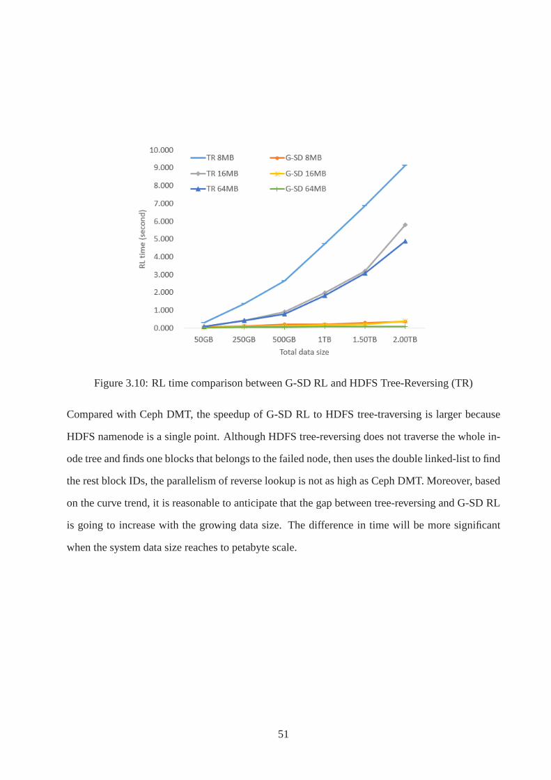
Figure 3.10: RL time comparison between G-SD RL and HDFS Tree-Reversing (TR)
Compared with Ceph DMT, the speedup of G-SD RL to HDFS tree-traversing is larger because
HDFS namenode is a single point. Although HDFS tree-reversing does not traverse the whole in-
ode tree and finds one blocks that belongs to the failed node, then uses the double linked-list to find
the rest block IDs, the parallelism of reverse lookup is not as high as Ceph DMT. Moreover, based
on the curve trend, it is reasonable to anticipate that the gap between tree-reversing and G-SD RL
is going to increase with the growing data size. The difference in time will be more significant
when the system data size reaches to petabyte scale.
51

CHAPTER 4: PERFECT ENERGY, RECOVERY AND PERFORMANCE
MODEL
4.1 Problem Formulation
In this section, we introduce “PERP” to explore the energy savings via adjusting recovery speed
and the number of spinning-up disks. In a normal energy/performance tradeoff, the usual optimiza-
tion goal is to minimize the energy consumption with respectto certain performance constraints.
While under degradation mode where recovery is initialized, there are three different requirements
that are mutually affected by the other two: energy efficiency, performance and recovery. For
example, to speed up the recovery, the system can: 1) activate more storage nodes to increase the
recovery parallelism, which will increase the energy consumption, or 2) assign more I/O bandwidth
to increase the recovery speed, which will have an adverse affect on the normal performance. Sim-
ilarly, 3) if we want to reduce the energy consumption, a certain number of disks need to be shut
down and this will decrease both performance and recovery speed. Given the knowledge of perfor-
mance constraints, our goal in PERP is to find a balance point between performance and recovery
speed that is able to minimize energy consumption within their constraints (see Section 4.1.2 for
detail).
4.1.1 Workload Model and Assumptions
We define the time interval of interest ast ∈ 1, 2, ..., T . Thus, the workload can be illustrated by
user request arrival rateλ(t). The variants we want to determine are: number of active disks in
storage systemsx(t) and recovery arrival rate (recovery speed)γ(t).
52
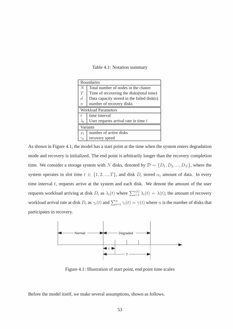
Table 4.1: Notation summary
BoundariesN Total number of nodes in the clusterT Time of recovering the disks(total time)d Data capacity stored in the failed disk(s)n number of recovery disks
Workload Parameterst time intervalλt User requests arrival rate in timet
Variantsxt number of active disksγt recovery speed
As shown in Figure 4.1, the model has a start point at the time when the system enters degradation
mode and recovery is initialized. The end point is arbitrarily longer than the recovery completion
time. We consider a storage system withN disks, denoted byD = {D1, D2, ..., DN}, where the
system operates in slot timet ∈ {1, 2, ..., T}, and diskDi storedαi amount of data. In every
time intervalt, requests arrive at the system and each disk. We denote the amount of the user
requests workload arriving at diskDi asλi(t) where∑x(t)
i=1 λi(t) = λ(t); the amount of recovery
workload arrival rate at diskDi asγi(t) and∑n
i=1 γi(t) = γ(t) wheren is the number of disks that
participates in recovery.
Normal Degraded
T
t
Figure 4.1: Illustration of start point, end point time scales
Before the model itself, we make several assumptions, shownas follows.
53
• In the model, we do not consider cascading failures, which means that there are no failures
happening during the recovery process.
• We assume the storage nodes are homogenous and the network transfer speed among each
node is the same. This means the recovery speeds for all nodesare the same.
4.1.2 The Energy Cost Model
As in degradation mode, adjusting one character among energy, performance and reliability will
automatically affects the other two. We are interested in identifying equilibrium points for the
following scenario: given certain performance constraints (required by SLA) and reliability con-
straints (required by the storage system) at each time slott, find the solution for the number of
active nodesx(t), and recovery speedγ(t) that is able to minimize the energy consumption during
the degradation process. Then, denote the overall throughput of one node as1 without loss of
generality. Mathematically, we can formulated
minimize E = EO + ES (4.1)
subject to λ(t) ≥ η, R(γ(t), l) = ξ (4.2)
0 ≤ x(t) ≤ N, ξ ≤ T
whereE is the total energy consumption during the recovery process; η is the performance con-
straint, andξ is the recovery time constraint, which means the recovery process should be com-
pleted by a certain amount of time.R(γ(t), l) is the recovery time function, which outputs the
time for recoveringl failed disks usingγ(t) recovery speed withinT total time. Our definitions
on performance constraint and recovery constraint are feasible due to the following reasons—first,
54
we define performance constraint based on SLA requirement, which can be measured in response
time or throughput. From the system perspective, each response time can be mapped into a spe-
cific throughput value. The mapping mechanism is introducedin paper [75]. Second, the recovery
constraint is defined based on recovery time, which means that the recovery process should be
completed within a certain amount of timeξ that is no longer thanT . Note that when deriving
functionR, both multi-disk failure and parallel recovery will be considered (see Section 4.1.4 for
details).
To model the storage system, operational energy costE consists of two major parts:Operational
energy cost(EO) and Switching energy cost(ES) [38]. Operational energy cost is the energy
consumption during operation time. According to literature [38], operational cost under normal
mode (with no failure) in a homogeneous server center can be modeled using a convex function
f(x(t), λi(t)) with x(t) active servers andλi(t) assigned throughput for nodei. This is because
all active storage nodes serves the user requests. However,when a node failure occurs, the sys-
tem will enter the degraded mode and wake up a certain number of storage nodes based on the
data layout schemes to conduct the recovery process. In thissituation, the storage nodes can be
easily divided into three parts—1) normal service nodes, which only serve normal user requests;
2) mixed nodes, which handles both normal user requests and the recovery process; and 3) re-
covery nodes, which only conduct recovery process to maintain the level of system reliability and
data availability. Here we model the operational energy cost using three time-varying functions:
f(x(t), λi(t))(i ∈ (n, x(t)]) for normal service nodes,g(x(t), λj(t), γj(t))(j ∈ (m,n]) for mixed
nodes, andh(x(t), γk(t))(k ∈ [1, m]) for recovery nodes. Together in time slott they usex(t)
active disks, serving a throughput ofλ(t) = λ1(t), λ2(t), ..., λx(t)(t) for incoming requests and
γ(t) = γ1(t), γ2(t), ..., γx(t)(t) for the recovery process. Thus, the energy costEO can be calcu-
lated as follows.
55

EO =T∑t=1
x(t)∑i=n
f(x(t), λi(t)) +T∑t=1
n∑j=m
g(x(t), λj(t), γj(t)) (4.3)
+T∑t=1
m∑k=1
h(x(t), γk(t))
In Equation 4.3,f andg can be considered calculated in two parts: compulsory energy cost and
service energy consumption.
It is well-acknowledged that the current Hard Disk Drive(HDD) has three states: busy, idle and
standby [28]. Busy state means the disk is serving requests,which includes rotating the disk’s
plate, seeking data parts and transferring data. While the disk is in idle state, it only spins the plate
without seeking. Standby mode means the disk is spun down, which consumes far less energy than
the previous two. In this model, we assume an active disk is either in idle or busy state; and each
disk is identical.
• Compulsory energy costis the energy consumption when the disk is not serving any requests
(only spinning the disk plate). As this operation is not related to the incoming requests, we
model it using a fixed parameterp for each disk. Thus, the compulsory energy consumption
for the whole storage system in time slott is p ∗ x(t).
• Servicing energy costis the energy consumption for serving the incoming requests(seeking,
accessing and transferring). Letq be the average energy consumption for each request, the
servicing energy cost for nodei is qλi(t) if node i is a normal service node (i ∈ [n, x(t)]);
q(λj(t) + γj(t)) if nodej is a mixed node (j ∈ [m,n]); qγk(t) if nodek is a recovery node
(k ∈ [1, m]). Especially, since both normal requests and recovery requests will arrive mixed
nodej with the arrival rate ofλj(t) andγj(t), respectively,q((λj(t) + γj(t)) calculates the
total energy consumption to deal with these request.
Combining them together, the operational energy cost for the three types of nodes can be calculated
56
as
f(x(t), λi(t)) = p+ qλi(t) (4.4)
g(x(t), λj(t), γj(t) = p+ q(λj(t) + γj(t)) (4.5)
h(x(t), γk(t)) = p+ qγk(t) (4.6)
wherep andq are constant numbers.
Note that we do not consider from the request level queueing delay as previous works did [38, 43]
due to the overlap between queueing time and service time among requests in each disk queueing
model, which we find unable to depict the scenario of the disk energy cost. In a typical storage
system, incoming requests will first be placed in a disk queuebefore being processed. For each
incoming request, the operational energy cost includes queueing delay-based energy costs and
service energy costs. However, when considering the energycost for each storage node in our
model, there is an overlap between queueing time and servicing time. e.g. when one request is
queued, it means other requests are under processing at thistime. Thus we believe simply adding
the queueing delay for each request together cannot accurately illustrate the scenario of our energy
cost model. Instead, we find the following affine functionf(λi(t)) = p + qλi(t) for modeling
energy cost in typical servers more suitable for modeling the storage system [38], wherep andq
are constant numbers that symbolize the parameters for two costs mentioned above.
The switching energy cost is the energy consumption for spinning the disks up and down. The
most straightforward way is to compute the differences between the active node number in time
slot t − 1 andt, which is|x(t) − x(t − 1)|. Here we define the energy cost of spinning one node
up asυ1 and the energy cost of spinning it down asυ2. ES can be modeled asS(x(t − 1), x(t)),
57
which is calculated as follows.
S(x(t− 1), x(t)) = υ1 ∗ [x(t)− x(t− 1)]+ + υ2 ∗ [x(t− 1)− x(t)]+ (4.7)
where[·]+ means that the result is[·] if it is positive and0 if it is negative. When deciding the
value ofυ1 andυ2, we consider the energy cost related to the switching up/down of the storage
nodes and calculate it based on its proportion to the constant energy consumption (of spinning a
disk)p during one time slot. For example, based on the results of ourtestbed, the time and energy
consumption for switching up a disk from the standby mode to active mode is10.9 seconds and
13.5 W , while switching down needs2 seconds and4.9 W . Thus the total energy consumption
of switching up and down one disk are13.5 × 10.9 = 147.15 J and2 × 4.9 = 9.8 J, respectively.
Since the energy consumption of the idle state isp = 10.2 W, the above two energy consumptions
equal to running the disk at idle state for14 and0.96 seconds. If each time slot is14 seconds, we
can setυ1 = 1 andυ2 = 0.07.
4.1.3 The PERP Minimization Problem
Based on the above models, the goal of this energy cost optimization problem is twofold. Subject
to performance and reliability constraints, the model is aiming to: 1) choose the optimal number
of active nodesx(t), and 2) assign the optimal recovery speedγ(t) in each time slott to minimize
58

the total energy consumption during the recovery time[1, T ]. Let γi(t) shown as follows.
min.T∑t=1
x(t)∑i=n
f(x(t), λi(t)) +T∑t=1
n∑j=m
g(x(t), γj(t), λj(t)) (4.8)
T∑t=1
m∑k=1
h(x(t), γk(t)) +T∑t=1
S(x(t− 1), x(t))
s.t. 0 ≤ m ≤ n ≤ x(t) ≤ N (4.9)
λi(t) ≤ 1, ∀i ∈ [n, x(t)] (4.10)
λj(t) + γj(t) ≤ 1, ∀j ∈ [m,n] (4.11)
γk(t) ≤ 1, ∀k ∈ [1, m] (4.12)
λ(t) ≥ η, R(γ(t), l) = ξ, ξ ≤ T (4.13)
where constraint 4.9 is setting the basic boundaries forx(t); constraint 4.10 to 4.12 define the
throughput bounds for each node; constraint 4.13 defines theperformance constraint that satisfies
the SLA requirement and recovery speed constraint that willmaintain the considerable level of
reliability, meaning the storage system should recover thefailed nodes in less than a certain amount
of time to limit the “time of vulnerability”.
We refer this optimization problem as Perfect Energy, Reliability, and Performance (PERP) Bal-
ance Problem in the remainder of this paper. Among all of the parameters, the input includes the
workloadλ, the data capacity of the failed nodeαi, and the failed node numberf . The recovery
node numbern is dependent on the data layout scheme. For example, in a chain-declustering data
layout with two-way replication,n is 2 for one data node failure. Note in this model, we do not
explicitly consider the bounds for the active node numberx(t) because we will see in Section 4.1.4
that x(t) will always have a relationship with the incoming workload based on constraint 4.10
and 4.11.
In contrast to the prior works which are focusing on trading off energy/performance, PERP is the
59
first, to the best of our knowledge, that incorporates reliability factors into the traditional ener-
gy/performance model, and jointly studies the relationships among these three key characteristics.
4.1.4 Solving PERP
By combining the previous Equations 4.4 and 4.6 together, the objective function 4.9 can be derived
as
min.T∑t=1
(x(t)∑i=n
qλi(t) +n∑
j=m
q(λj(t) + γj(t)) +m∑k=1
qγk(t)
)(4.14)
+T∑t=1
px(t) +T∑t=1
S(x(t− 1), x(t))
which subjects to the same constraints from 4.9 to 4.13. To simplify the object function, we merge
the polynomial in 4.14.
min.T∑t=1
(px(t) + qλ(t) + qγ(t)) +T∑t=1
S(x(t− 1), x(t)) (4.15)
whereλ(t) andγ(t) are the summations of eachλ∗(t) andγ∗(t), respectively. DefineF (x(t), λ(t), γ(t)) =T∑t=1
(px(t) + qλ(t) + qγ(t)), the object function turns into the function ofx(t), λ(t) andγ(t) in-
stead ofλi(t) andγi(t).
Now we want to reducei andj in constraints 4.10 to 4.12, so that they coincide with the merged
object function 4.15.
Lemma 1 Denoteν∗i (t) wherei ∈ {1, 2, ..., x(t)} as the optimal workload assignment for nodei
at time slott. Thenν1(t) = ν2(t) = ... = νx(t)(t) =λ(t)+γ(t)
x(t).
PROOF. As aforementioned, in a system withx active nodes andν total request rates, the opera-
60
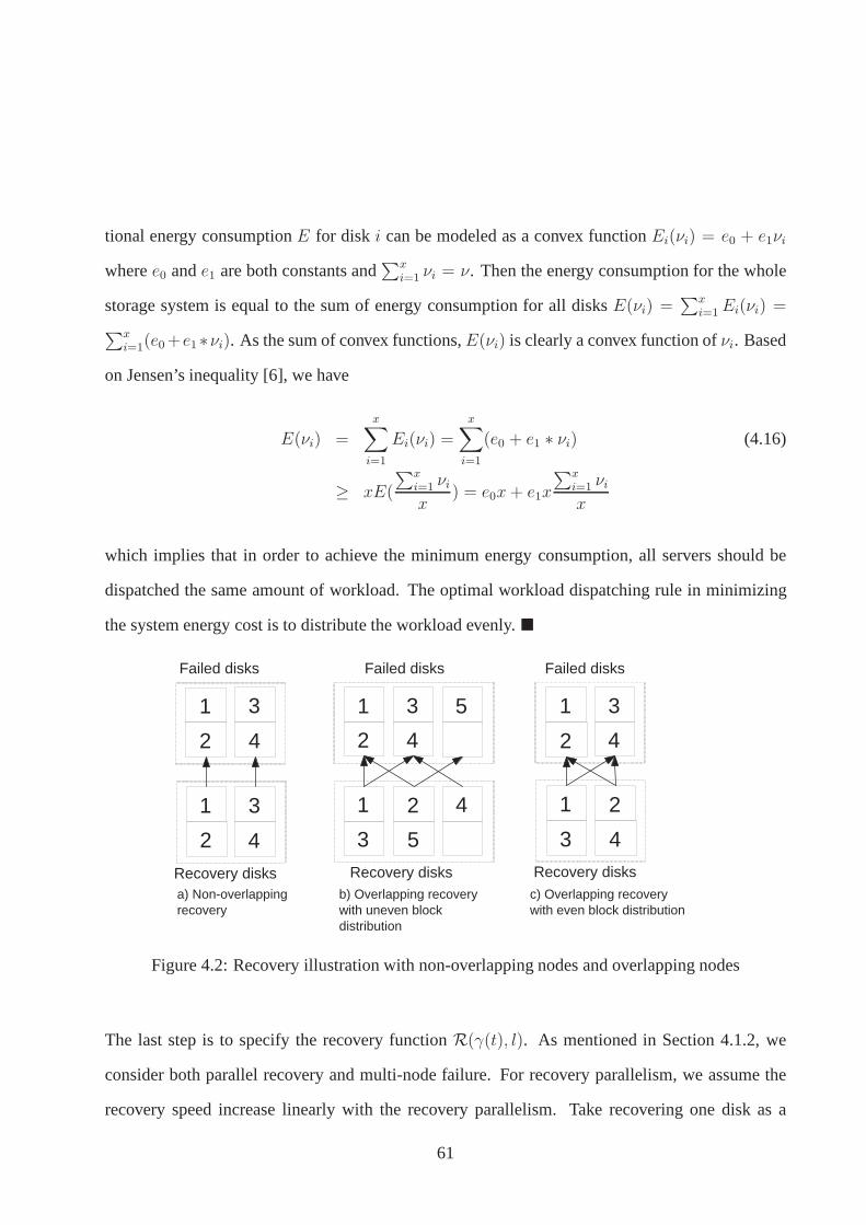
tional energy consumptionE for disk i can be modeled as a convex functionEi(νi) = e0 + e1νi
wheree0 ande1 are both constants and∑x
i=1 νi = ν. Then the energy consumption for the whole
storage system is equal to the sum of energy consumption for all disksE(νi) =∑x
i=1Ei(νi) =
∑xi=1(e0+e1∗νi). As the sum of convex functions,E(νi) is clearly a convex function ofνi. Based
on Jensen’s inequality [6], we have
E(νi) =
x∑
i=1
Ei(νi) =
x∑
i=1
(e0 + e1 ∗ νi) (4.16)
≥ xE(
∑xi=1 νix
) = e0x+ e1x
∑xi=1 νix
which implies that in order to achieve the minimum energy consumption, all servers should be
dispatched the same amount of workload. The optimal workload dispatching rule in minimizing
the system energy cost is to distribute the workload evenly.�
1
2
Failed disks
Recovery disks a) Non-overlapping recovery
c) Overlapping recovery with even block distribution
b) Overlapping recovery with uneven block distribution
3
4
1
2
3
4
1
2
Failed disks
Recovery disks
3
4
1
3
2
4
1
2
Failed disks
Recovery disks
3
4
1
3
2
5
5
4
Figure 4.2: Recovery illustration with non-overlapping nodes and overlapping nodes
The last step is to specify the recovery functionR(γ(t), l). As mentioned in Section 4.1.2, we
consider both parallel recovery and multi-node failure. For recovery parallelism, we assume the
recovery speed increase linearly with the recovery parallelism. Take recovering one disk as a
61

simple example, two-disk parallel recovery will double therecovery speed of one disk recovery.
Mathematically, it is easy to get∑ξ
t=1 γ(t) = d from 4.13 due to all recovery speed contributing
to reconstruct one disk. When there are multi-node failuresin the system, there are two basic
situations:
1. The failed nodes are recovered onnon-overlapping nodes, as shown in Figure 4.2 a). Based
on the weakest link principle [9], the total recovery time isdecided by the longest recovery
time of each failed node (ξ = max(T1, T2, ...Tl) whereT∗ is the recovery time for each failed
disk). We prove that the recovery time is minimized whenT1 = T2 = ... = ξ, as shown
in Lemma 1. In this scenario, we can sum up and get∑ξ
t=1 γ(t) = d, whered is the total
amount of data to be recovery.
2. The failed nodes are recovered byoverlapping nodes, as shown in Figure 4.2 b) and c). The
total recovery time is decided by the shortest time of all possible combinations (ξ = min(all
possible recovery combinations)). Using same proof,T1 = T2 = ... = ξ can achieve the
minimum recovery time, where we can get∑ξ
t=1 γ(t) = d.
Theorem 1 Let d =∑l
i=1 γi(t)Ti andγ(t) =∑l
i=1 γi(t). T = max{T1, T2 . . . Tl}. We will get
minimum recovery timeT whenT1 = T2 = · · · = Tl.
PROOF. We prove it by enumerating all possible cases. Asγ(t) =∑l
i=1 γi(t), we haveγ1(t) =
γ(t)− γ2(t)− · · · − γl(t). Then
d = (γ(t)− γ2(t)− · · · − γl(t))T1 + γ2(t)T2 + · · ·+ γl(t)Tl (4.17)
= γ(t)T1 + γ2(t)(T2 − T1) + · · ·+ γl(t)(Tl − T1).
Case 1:T1 = T2 = · · · = Tl, we haveT = T1 = T2 · · · = Tl andd = γ(t)T1. This implies
62
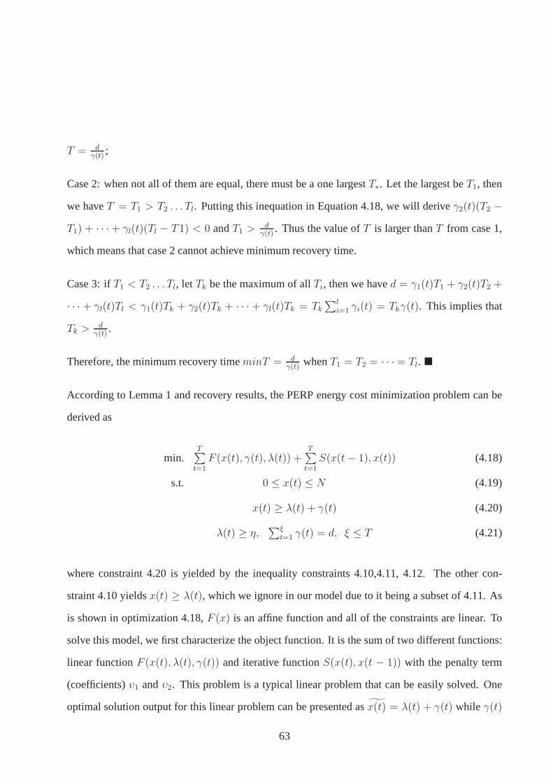
T = dγ(t)
;
Case 2: when not all of them are equal, there must be a one largestT∗. Let the largest beT1, then
we haveT = T1 > T2 . . . Tl. Putting this inequation in Equation 4.18, we will deriveγ2(t)(T2 −
T1) + · · · + γl(t)(Tl − T1) < 0 andT1 > dγ(t)
. Thus the value ofT is larger thanT from case 1,
which means that case 2 cannot achieve minimum recovery time.
Case 3: ifT1 < T2 . . . Tl, let Tk be the maximum of allTi, then we haved = γ1(t)T1 + γ2(t)T2 +
· · · + γl(t)Tl < γ1(t)Tk + γ2(t)Tk + · · · + γl(t)Tk = Tk
∑li=1 γi(t) = Tkγ(t). This implies that
Tk > dγ(t)
.
Therefore, the minimum recovery timeminT = dγ(t)
whenT1 = T2 = · · · = Tl. �
According to Lemma 1 and recovery results, the PERP energy cost minimization problem can be
derived as
min.T∑t=1
F (x(t), γ(t), λ(t)) +T∑t=1
S(x(t− 1), x(t)) (4.18)
s.t. 0 ≤ x(t) ≤ N (4.19)
x(t) ≥ λ(t) + γ(t) (4.20)
λ(t) ≥ η,∑ξ
t=1 γ(t) = d, ξ ≤ T (4.21)
where constraint 4.20 is yielded by the inequality constraints 4.10,4.11, 4.12. The other con-
straint 4.10 yieldsx(t) ≥ λ(t), which we ignore in our model due to it being a subset of 4.11. As
is shown in optimization 4.18,F (x) is an affine function and all of the constraints are linear. To
solve this model, we first characterize the object function.It is the sum of two different functions:
linear functionF (x(t), λ(t), γ(t)) and iterative functionS(x(t), x(t − 1)) with the penalty term
(coefficients)υ1 andυ2. This problem is a typical linear problem that can be easily solved. One
optimal solution output for this linear problem can be presented asx(t) = λ(t) + γ(t) while γ(t)
63
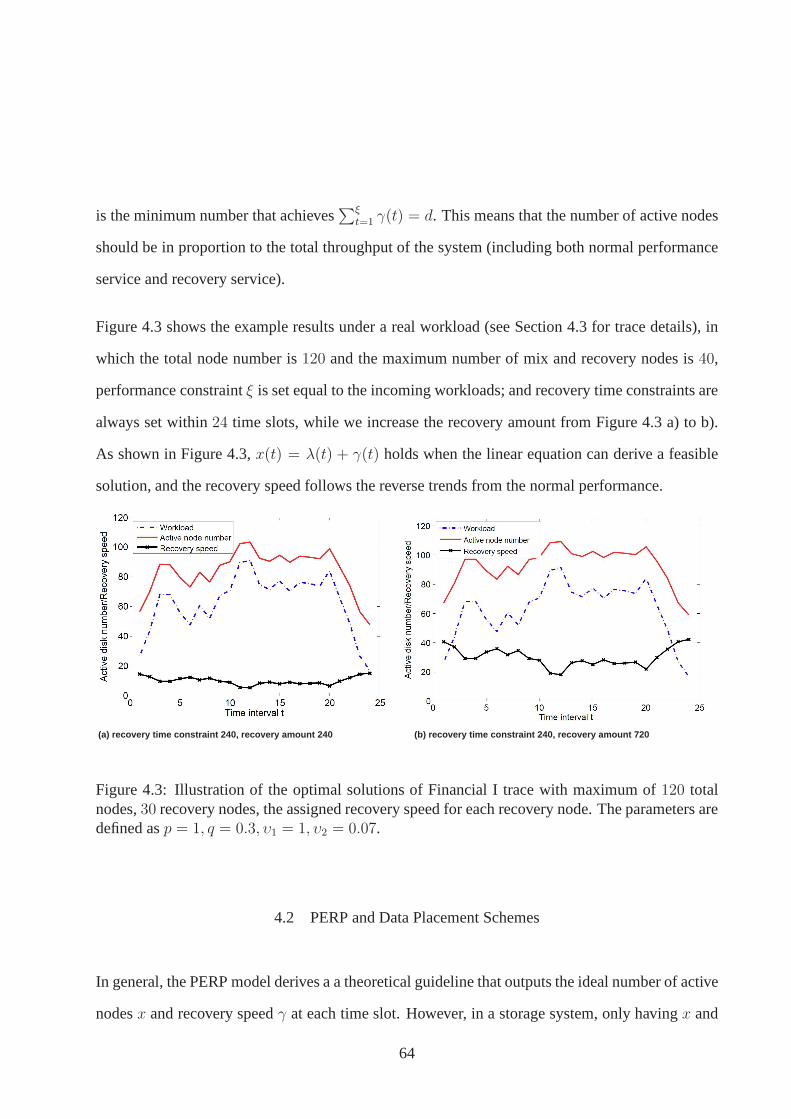
is the minimum number that achieves∑ξ
t=1 γ(t) = d. This means that the number of active nodes
should be in proportion to the total throughput of the system(including both normal performance
service and recovery service).
Figure 4.3 shows the example results under a real workload (see Section 4.3 for trace details), in
which the total node number is120 and the maximum number of mix and recovery nodes is40,
performance constraintξ is set equal to the incoming workloads; and recovery time constraints are
always set within24 time slots, while we increase the recovery amount from Figure 4.3 a) to b).
As shown in Figure 4.3,x(t) = λ(t) + γ(t) holds when the linear equation can derive a feasible
solution, and the recovery speed follows the reverse trendsfrom the normal performance.
(a) recovery time constraint 240, recovery amount 240 (b) recovery time constraint 240, recovery amount 720
Figure 4.3: Illustration of the optimal solutions of Financial I trace with maximum of120 totalnodes,30 recovery nodes, the assigned recovery speed for each recovery node. The parameters aredefined asp = 1, q = 0.3, υ1 = 1, υ2 = 0.07.
4.2 PERP and Data Placement Schemes
In general, the PERP model derives a a theoretical guidelinethat outputs the ideal number of active
nodesx and recovery speedγ at each time slot. However, in a storage system, only havingx and
64

γ is not enough for practical usage because data layout is the basis of the model. As PERP makes
several mathematical assumptions and ignore the block location information when retrieving the
optimal solution, the results may not be applicable in some data layouts. For example, the ran-
dom data layout, in which objects are randomly distributed to each node, cannot work with PERP
because shutting down any three disks will have99.9% probability of resulting in data unavail-
ability [16]. In this section, we first explicitly specify the PERP assumptions and implications.
Second, we study the adaptability of PERP on four different data layouts: group-rotational [22],
shifted-declustering [77] and power proportional layoutssuch as Sierra “power-aware” layout [56]
and Rabbit “equal-workload” layout [15]. Finally we provide an algorithm of choosing active
nodes based on PERP indicatedx and the applicable layouts.
4.2.1 PERP Properties
PERP is solved using two assumptions—even workload and equal time recovery. Also, the optimal
solution of active node number followsx(t) = λ(t) + γ(t). We summarize them as preconditions
for data layouts to achieve the PERP optimal solution. In this section, we explicitly define the
preconditions and explain how it is related to data layouts.
• Precondition 1 Even workload: as defined in Theorem 1, the power cost will be minimized
if each node shares the same amount of workload.
• Precondition 2 Equal time recovery: In a multiple node reconstruct scenario, the recovery
time is minimized if the recovery time for each failed node isthe same.
• Precondition 3 Power proportional: In degradation mode, the PERP solutionx(t) = λ(t) +
γ(t) indicates that the number of active nodes should be in proportion to the total I/O
throughput, which includes both normal performance and recovery. In normal mode with-
65
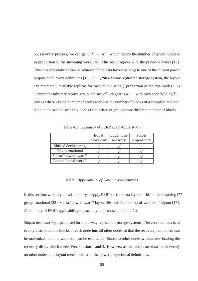
out recovery process, we can getx(t) = λ(t), which means the number of active nodes is
in proportion to the incoming workload. This result agrees with the previous works [17].
Thus this precondition can be achieved if the data layout belongs to one of the current power
proportional layout definitions [15, 56]. 1) “in ak-way replicated storage system, the layout
can maintaing available replicas for each chunk usinggk
proportion of the total nodes.” 2)
“Except the arbitrary replica group, the size ofr-th gear isper−1 with each node holdingB/i
blocks wherei is the number of nodes andB is the number of blocks of a complete replica.”
Note in the second scenario, nodes from different groups store different number of blocks.
Table 4.2: Summary of PERP adaptability study
Equal Equal time Powerworkload recovery proportional
Shifted declustering√ √ ×
Group rotational√ √ √
Sierra “power-aware”√ √ √
Rabbit “equal work”√ √ √
4.2.2 Applicability of Data Layout Schemes
In this section, we study the adaptability to apply PERP on four data layouts: shifted-declustering [77],
group-rotational [22], Sierra “power-aware” layout [56] and Rabbit “equal-workload” layout [15].
A summary of PERP applicability on each layout is shown in Table 4.2.
Shifted declusteringis proposed for multi-way replication storage systems. Theessential idea is to
evenly distributed the blocks of each node into all other nodes so that the recovery parallelism can
be maximized and the workload can be evenly distributed to other nodes without overloading the
recovery disks, which meets Precondition1 and2. However, as the blocks are distributed evenly
on other nodes, this layout meets neither of the power proportional definitions.
66
(1,1)
(4,1)
(7,1)
(2,1)
(5,1)
(8,1)
(3,1)
(6,1)
(9,1)
Group 1
Node 1 Node 2
(1,2)
(6,2)
(8,2)
(2,2)
(4,2)
(9,2)
(3,2)
(5,2)
(7,2)
(1,3)
(5,3)
(9,3)
(2,3)
(6,3)
(7,3)
(3,3)
(4,3)
(8,3)
Group 2 Group 3
Node 3 Node 4 Node 5 Node 6 Node 7 Node 8 Node 9
Figure 4.4: Example of Group-rotational Declustering DataLayout with9 total nodes,3 replicagroups
Group rotational declusteringwas first introduced to improve the performance of standard mir-
roring, and then extended to multi-way replication for highthroughput media server systems. It
partitions all disks into several groups, and the number of groups equals to the number of data
copies. Each group stores a complete copy of all the data.Sierra “power-aware” layoutis pro-
posed to increase the recovery parallelism with respect to power proportionality, which naturally
satisfies power proportional condition. Similar to group rotational layout, it also involves declus-
tering technique to distribute blocks evenly among the recovery nodes to improve the recovery
parallelism.
PERP can work with both layouts because 1) they both maintainthe same number of blocks in each
node. If the workload is distributed unbiased, the workloadis even, which satisfies Precondition
1. 2) the blocks are replicated evenly on a group of nodes, which means that the blocks from the
failed data node will be recovered evenly, leading to equal time recovery (satisfying precondition
2). 3) They meet the first power proportional condition—the nodes can be divided intok (replica
number) groups with each group containing a complete replica set.
Rabbit “equal work” layoutwas presented as an “ideal” power proportional layout with each node
containingB/i number of blocks. when openingx disks in this layout, each node can provide
an equalB/x blocks, which means each node is sharingx fraction of the whole workload. This
satisfies precondition3 naturally. Also, the replicas of each block are placedrandomlyinside the
67

“recovery group”, which means the recovery time for recovering the failed node is statistically
equal (satisfy Precondition1). Finally, Precondition2 is also satisfied because even if the nodes in
different gear fails, it is possible to schedule the recovery bandwidth so that each failed node can
be recovered in the same time.
4.2.3 Selecting the Active Nodes
This section presents anGradual Increasing/Decreasing Algorithmthat can specifyx(t) number
of active nodes at each time framet based on data layouts. The basic idea is to increase/decrease
the number of active nodes gradually with the various performance/recovery requirements. At time
slot t, one of the following four scenarios can happen,
1. Case 1: Required number of active nodes increasingx(t) ≥ x(t−1) and recovery bandwidth
increasingγ(t) ≥ γ(t− 1) means both normal performance and recovery requires a higher
throughput. As the recovery islocation-dependent, our algorithm first active the nodes that
is able to recover the failed nodes, and then increase the number of nodes correspondingly
based onx(t).
2. Case 2: Required number of active nodes increasingx(t) ≥ x(t−1) and recovery bandwidth
reducingγ(t) < γ(t − 1) means that the normal performance requires a higher throughput
while the recovery process can satisfy the requirement and have room to be slowed down at
time slott. In this case, we can first active normal performance nodes and then the nodes
that can participate in recovery.
3. Case 3: Required number of active nodes increasingx(t) < x(t−1) and recovery bandwidth
increasingγ(t) < γ(t−1) means that the system can be adjusted to a lower power state with
both performance and recovery requirement reducing. To achieve this, we first seek to spin
68
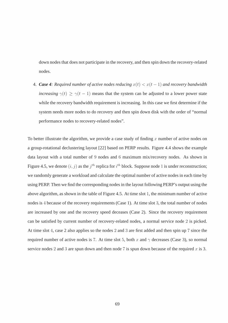
down nodes that does not participate in the recovery, and then spin down the recovery-related
nodes.
4. Case 4: Required number of active nodes reducingx(t) < x(t− 1) and recovery bandwidth
increasingγ(t) ≥ γ(t − 1) means that the system can be adjusted to a lower power state
while the recovery bandwidth requirement is increasing. Inthis case we first determine if the
system needs more nodes to do recovery and then spin down diskwith the order of “normal
performance nodes to recovery-related nodes”.
To better illustrate the algorithm, we provide a case study of finding x number of active nodes on
a group-rotational declustering layout [22] based on PERP results. Figure 4.4 shows the example
data layout with a total number of9 nodes and6 maximum mix/recovery nodes. As shown in
Figure 4.5, we denote(i, j) as thejth replica forith block. Suppose node1 is under reconstruction;
we randomly generate a workload and calculate the optimal number of active nodes in each time by
using PERP. Then we find the corresponding nodes in the layoutfollowing PERP’s output using the
above algorithm, as shown in the table of Figure 4.5. At time slot 1, the minimum number of active
nodes is4 because of the recovery requirements (Case 1). At time slot3, the total number of nodes
are increased by one and the recovery speed deceases (Case 2). Since the recovery requirement
can be satisfied by current number of recovery-related nodes, a normal service node2 is picked.
At time slot4, case 2 also applies so the nodes2 and3 are first added and then spin up7 since the
required number of active nodes is7. At time slot5, bothx andγ decreases (Case 3), so normal
service nodes2 and3 are spun down and then node7 is spun down because of the requiredx is 3.
69
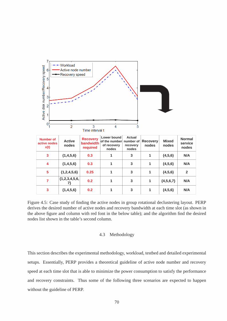
Number of active nodes
x(t)
Active nodes
Recovery bandwidth required
Lower bound of the number
of recovery nodes
Actual number of recovery
nodes
Recovery nodes
Mixed nodes
Normal service nodes
3 {1,4,5,6} 0.3 1 3 1 {4,5,6} N/A
4 {1,4,5,6} 0.3 1 3 1 {4,5,6} N/A
5 {1,2,4,5,6} 0.25 1 3 1 {4,5,6} 2
7 {1,2,3,4,5,6, 7} 0.2 1 3 1 {4,5,6,7} N/A
3 {1,4,5,6} 0.2 1 3 1 {4,5,6} N/A
Figure 4.5: Case study of finding the active nodes in group rotational declustering layout. PERPderives the desired number of active nodes and recovery bandwidth at each time slot (as shown inthe above figure and column with red font in the below table); and the algorithm find the desirednodes list shown in the table’s second column.
4.3 Methodology
This section describes the experimental methodology, workload, testbed and detailed experimental
setups. Essentially, PERP provides a theoretical guideline of active node number and recovery
speed at each time slot that is able to minimize the power consumption to satisfy the performance
and recovery constraints. Thus some of the following three scenarios are expected to happen
without the guideline of PERP.
70

• Performance requirement cannot be reached.
• Recovery requirement cannot be achieved.
• Performance and recovery constraints are both satisfied butmore power is consumed.
This power cost function is characterized by four parameters: p, q, υ1 andυ2. Same with the
parameters used in Figure 4.3, we choosep = 1, q = 0.3, υ1 = 1 andυ2 = 0.6.
Workload Our experiments are driven by an OLTP I/O trace named Financial I trace, which is
a typical storage I/O traces from the UMass Trace Repository[14]. This trace is collaboratively
collected by HP and the Storage Performance Council. The workload statistics are shown in Fig-
ure 4.3. In our experimental setup, we make necessary a speedup(∗120) so that the workload can
be applied into our testbed.
Table 4.3: CASS Cluster Configuration
Node ConfigurationsMake & Model Dell PowerEdge 1950CPU 2 Intel Xeon 5140, Dual Core,
2.23 GHzRAM 4.0 GB DDR2, PC2-5300, 667 MHzInternal HD 2 SATA 500 GB (7200RPM) or
2 SAS 147 GB (15K RPM)Network Connection Intel Pro/1000 NICOperating System Rocks 5.0 (Cent OS 5.1), Kernel:
2.6.1853.1.14.e15Cluster NetworkSwitch Make & Model Nortel BayStack 5510-48T Gigabit
Switch
Testbed The experiments are set up in our CASS cluster, which includes one rack of25 nodes(one
head node and24 compute nodes). Each node has its own internal storage. Table 4.3 shows the
CASS cluster configuration. In our experiment, we use head nodes as a central control and operate
the internal storage from all other nodes using remotefs [10]. We configure the compute nodes as
servers and head node as a client so that the head node can mount all internal disks of the compute
71
nodes. When closing the storage nodes, they are set to hibernate state which consumes4 W. Each
node is configured to store80 GB data with a block size100 MB. In the following experiments,
two nodes are assumed to be under reconstruction, which is160 GB in total.
Trace Replay Framework A simulation framework was developed to replay traces and operate on
the disks based on the trace workload. The trace replay framework is implemented, which has2k C
code. The main idea of this framework is to use “Libaio” programming library to asynchronously
access the I/O of each storage node (sending read/write requests).
The trace replay framework consists of six key components: trace parser, replay driver, data layout,
node manager, recovery thread and I/O scheduler. Among them, the trace parser interprets different
kinds of trace formats. The replay driver interacts with thedisks and sends the traces to the layout
module. The data layout policy defines the mapping algorithms from logical addresses to the
physical address. The node manager reads the PERP output andadjusts node status based onx. The
recovery thread simulates the recovery process by sending “write” requests to reconstructed nodes
and sending “read” requests to mix/recovery nodes. I/O scheduler also reads from PERP output
recovery speed and tries to assign recovery workloads evenly on the mix/recovery nodes. In our
experiments, we implement Sierra “power-aware” data layout and group-rotational declustering
layout as the initial data layout. In order to test PERP outputs with other configurations. It requires
the active node numberx to exactly follows the PERP results. Thus the node manager will not
open nodes as the example shown in Section 4.2.3. Instead, itfirst maintains one copy of the whole
dataset and opens up the corresponding number of nodes without considering the data location.
Baselines We compare PERP with two power proportional work: Sierra, which aims to maximize
the recovery parallelism (speed) and Rabbit, which recovers the failed data using a fixed number
of nodes within a recovery group. We implement the data layouts in the simulation framework,
mimic their policies and compared the power, performance and recovery with PERP on our CASS
72
cluster.
4.4 Experiments
In this section, we present the experiment results. To provethe effectiveness of PERP, the following
tests are conducted. First, we validate PERP’s optimality by changing one of its outputs while
fixing the other one. This includes two scenarios:fixedx, variedγ or fixedγ, variedx. Second,
we compare PERP with baseline policies abstracted from Sierra [56], which is trying to maximize
the recovery parallelism (speed).
4.4.1 PERP optimality
This set of experiments is aiming to show that the PERP outputsx(t) andγ(t) at each time slot are
optimal. We first output the desiredx(t) (number of active nodes) andγ(t) (recovery speed) based
on24 nodes and incoming workloads, then we compare the performance, energy consumption with
fixing one output while adjust the other.
4.4.1.1 PERPvs. Fixed recovery speedγ, varied active node numberx
In these experiments, we compare the power and performance for PERP outputs (active node
numberx, recovery speedγ) with fixed recovery speed, varied number of active nodes, denoted
asx′. There are three possibilities forx′: 1) x′ < x meansx′(t) as active node number is smaller
thanx(t) at each time frame. 2)x′ > x, means allx′(t) is larger thanx(t) at each time slot. 3)
x′ <> x, meansx′(t) is smaller thanx(t) at some time frames while larger thanx(t) at other
time frames. Fromx(t) = λ(t) + γ(t), we can easily tell that scenario 1) and 3) are not feasible
73
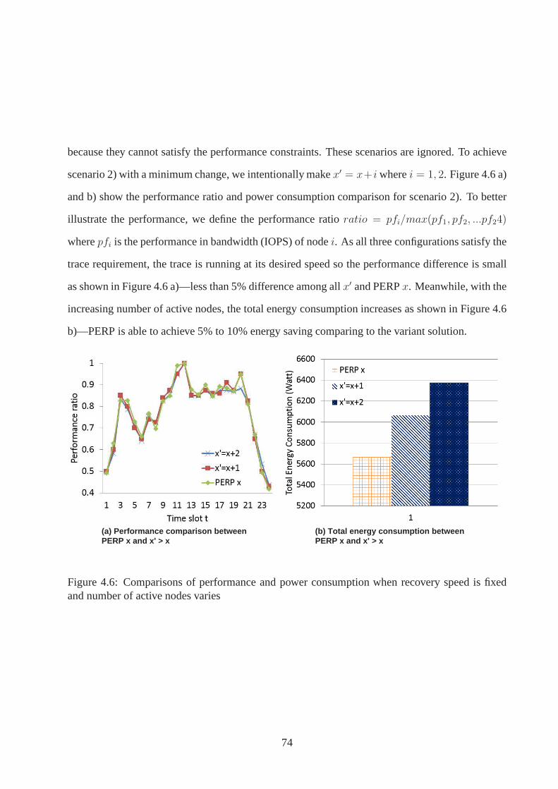
because they cannot satisfy the performance constraints. These scenarios are ignored. To achieve
scenario 2) with a minimum change, we intentionally makex′ = x+i wherei = 1, 2. Figure 4.6 a)
and b) show the performance ratio and power consumption comparison for scenario 2). To better
illustrate the performance, we define the performance ratioratio = pfi/max(pf1, pf2, ...pf24)
wherepfi is the performance in bandwidth (IOPS) of nodei. As all three configurations satisfy the
trace requirement, the trace is running at its desired speedso the performance difference is small
as shown in Figure 4.6 a)—less than 5% difference among allx′ and PERPx. Meanwhile, with the
increasing number of active nodes, the total energy consumption increases as shown in Figure 4.6
b)—PERP is able to achieve 5% to 10% energy saving comparing to the variant solution.
(a) Performance comparison between PERP x and x' > x
(b) Total energy consumption between PERP x and x' > x
Figure 4.6: Comparisons of performance and power consumption when recovery speed is fixedand number of active nodes varies
74

4.4.1.2 PERPvs. Fixed active node numberx, varied recovery speedγ
In this experiment, we compare the power and recovery statusbetween PERPx andγ and fixed
x and variedγ, which we refer as “γ′”. Similar with above,γ′ has three possibilities: 1)γ′ <
γ, means the varied recovery speed at each time slotγ(t) is always less than PERPγ(t). This
scenario is apparently not possible because it violates therecovery requirements. 2)γ′ > γ,
meansγ′(t) is always larger thanγ(t) at each time slot. As the active node number is fixed and
x(t) = λ(t)+γ(t), increasingγ(t) will decrease the performance, which will result in violating the
performance constraint. 3)γ′ <> γ, meansγ′(t) in some time frames is larger thanγ(t) while in
other time frames it is smaller thanγ(t). This scenario is also not feasible because the performance
requirement will not be met whenγ′(t) > γ(t). All scenarios violates the constraints thus proving
the optimality of PERP outputs.
4.4.2 Comparison between PERP, Maximum Recovery and Recovery Group
In this section, we compare PERP with two recovery policies abstracted from current power pro-
portional works: Maximum Recovery (MR) policy abstracted from “Sierra”, and Recovery Group
(RG) policy abstracted from “Rabbit”. The key idea of MR is toachieve maximum recovery par-
allelism (speed), which isN/3 in aN total nodes with three-way replication system. That means,
all of the nodes that are participated in the recovery (maximum16 nodes in our testbed) should be
opened and the recovery speed for each mix/recovery node should be1 (1300 IOPS). In Rabbit,
the recovery group size is determined by the gear sizegsize and number of primary nodespsize
according to the equationgroupS = e(psize−gsize)−psizegsize
. According to Rabbit’s calculation, in a
25-node cluster, the size of the primary group is3, the number of nodes in the second replica is
6, and the number of nodes in the third replica group is16. Thus with the gear size of1, the
size of recovery group can be calculated as6, which we use for the following sets of experiments.
75

We compare these two policies with PERP on recovery speed, number of recovery nodes, energy
consumption and normal performance. Note if the normal performance can not be met even with
all nodes activated, the I/O scheduler will prioritize the normal performance instead of recovery.
We conduct experiments with two recovery amount configurations, one with 3 disks and 240GB
needed to be recovered, and the other one with 4 disks and 320GB needed to be recovered.
(a) Recovery speed comparison (b) Number of active nodes comparison
(c) Energy consumption comparison (d) Performance comparison
Figure 4.7: Comparison of recovery speed, performance, energy consumption and number of activenodes between PERP, MR and RG when recovery amount is 240GB
The results shown in Figure 4.7 and 4.8 illustrate the comparison between PERP, MR and RG in
recovery speed, number of active nodes, power consumption and normal performance. In both
sets of experiments, to achieve the maximum recovery speed while maintaining a certain level of
performance constraint, MR opens up all recovery-related nodes in the first several time slots.e.g.
7 time slots for 240GB test and8 time slots for 320GB test. After that, when all recovery processes
are completed, it goes back to normal mode following its power proportional layout solution. RG
on the other hand, activates one recovery group with 6 fixed number of disks to recover the failed
76
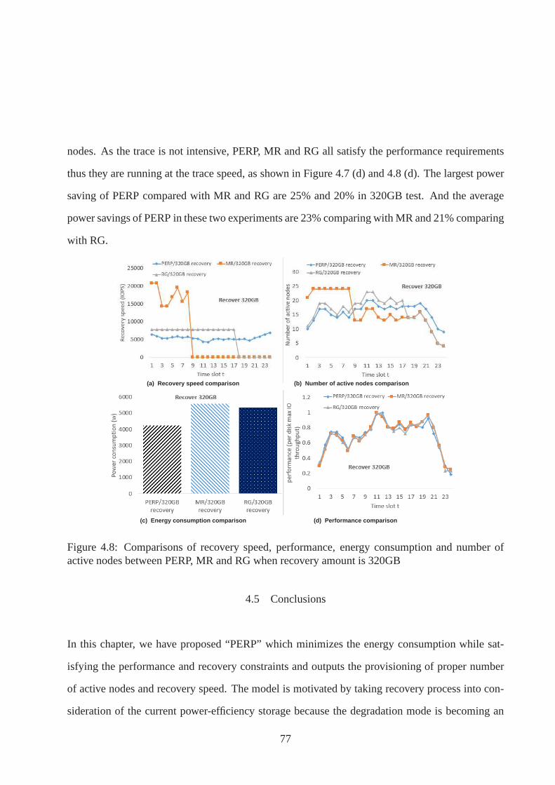
nodes. As the trace is not intensive, PERP, MR and RG all satisfy the performance requirements
thus they are running at the trace speed, as shown in Figure 4.7 (d) and 4.8 (d). The largest power
saving of PERP compared with MR and RG are 25% and 20% in 320GB test. And the average
power savings of PERP in these two experiments are 23% comparing with MR and 21% comparing
with RG.
(a) Recovery speed comparison (b) Number of active nodes comparison
(c) Energy consumption comparison (d) Performance comparison
Figure 4.8: Comparisons of recovery speed, performance, energy consumption and number ofactive nodes between PERP, MR and RG when recovery amount is 320GB
4.5 Conclusions
In this chapter, we have proposed “PERP” which minimizes theenergy consumption while sat-
isfying the performance and recovery constraints and outputs the provisioning of proper number
of active nodes and recovery speed. The model is motivated bytaking recovery process into con-
sideration of the current power-efficiency storage becausethe degradation mode is becoming an
77

non-neglectable operational state, which is overlooked byprevious researches. We summarize the
preconditions of deriving PERP results and study the applicability of working with current data lay-
outs. Group-rotational declustering layout is studied as an example of choosing the proper nodes
to activate. According to the comprehensive experiments onthe in-house CASS cluster with25
nodes, we first prove the optimality by comparing PERP with various configurations based on the
original output. Moreover, experiments of comparing PERP with the maximum recovery policy
and recovery group policy indicate that with satisfying both performance and recovery constraints,
our solution saves up to 25% and 20%, respectively.
78
CHAPTER 5: DEISTER: A LIGHT-WEIGHT BLOCK MANAGEMENT
SCHEME
Deister is built upon an architecture that consists ofM (M ≥ 1) master nodes andN (N >> M)
data nodes, where each node has one or more locally attached disks for storing data. The master
nodes and data nodes are connected by high-speed network switches in a local area network. We
refer each logical data unit as a block. Each master node manages a single namespace, which does
not need any coordinations with other master nodes.
Before the design, we define several terminologies, as follows.
1. Theredundancy setis the set of one block and all its replicas.
2. TheISD nodeis a group of blocks that belongs to one physical data node. Each physical
node can have multiple ISD nodes.
3. TheLogic groupcontains a group of ISD nodes, in which the block to node mapping is
realized using SD layout.
4. Thereverse lookupis the process of finding the whole block list that resides on this data
node given a data node ID.
5.1 Overall Design
The Intersected Shifted Declustering distribution algorithm is extended from our previous work
Shifted Declustering (SD) [77, 72], which is an ideal declustering data placement algorithm [77]
and can reach at most(n − 1) parallelism in node reconstruction. Similar to other deterministic
layouts, both data distribution and data lookup is derived using the placement algorithm, which can
79
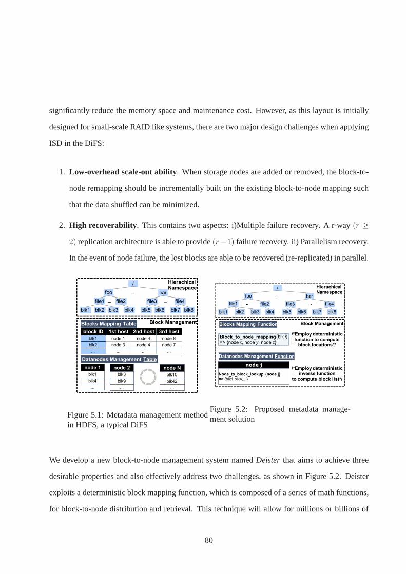
significantly reduce the memory space and maintenance cost.However, as this layout is initially
designed for small-scale RAID like systems, there are two major design challenges when applying
ISD in the DiFS:
1. Low-overhead scale-out ability. When storage nodes are added or removed, the block-to-
node remapping should be incrementally built on the existing block-to-node mapping such
that the data shuffled can be minimized.
2. High recoverability . This contains two aspects: i)Multiple failure recovery. Ar-way (r ≥
2) replication architecture is able to provide(r−1) failure recovery. ii) Parallelism recovery.
In the event of node failure, the lost blocks are able to be recovered (re-replicated) in parallel.
block ID 1st host 2nd host 3rd host
blk1 node 1 node 4 node 8
blk2 node 3 node 4 node 7
... ... ... ...
node 1
blk1
blk4
...
Block ManagementBlocks Mapping Table
Datanodes Management Table
HierachicalNamespace
/
foo bar
file1 file2 file3 file4
blk1 blk2 blk3 blk4 blk5 blk6 blk7 blk8
Node_to_block_lookup=>
Datanodes Management
node 2
blk3
blk9
...
node N
blk10
blk42
...
Blocks Mapping
blk1
...
... ...
Figure 5.1: Metadata management methodin HDFS, a typical DiFS
Block Management
HierachicalNamespace
file4
blk8
node j
Node_to_block_lookup (node j)=> {blk1,blk4,...}
Datanodes Management Function
Block_to_node_mapping(blk i)
=> {node x, node y, node z}
Block Management
/*Employ deterministicfunction to compute
block locations*/
/*Employ deterministicinverse function
to compute block list*/
Blocks Mapping Function
HierachicalNamespace
/
foo bar
file1 file2 file3 file4
blk1 blk2 blk3 blk4 blk5 blk6 blk7 blk8
Figure 5.2: Proposed metadata manage-ment solution
We develop a new block-to-node management system namedDeister that aims to achieve three
desirable properties and also effectively address two challenges, as shown in Figure 5.2. Deister
exploits a deterministic block mapping function, which is composed of a series of math functions,
for block-to-node distribution and retrieval. This technique will allow for millions or billions of
80
block-to-node records to be removed. Therefore, Deister will achieve light-weight block manage-
ment for large-scale data-intensive file systems, e.g, HDFS. Deister consists of a block distribution
scheme, Intersected Shifted Declustering mapping and its corresponding block management.
1) Intersected SD Mapping adds an abstract mapping layer named Logic Group (LG) between
the original block-to-node mapping. Each data node can belong to multiple logic groups and
blocks are mapped to these groups before they are placed on the data nodes. Thus while the block
distribution and lookup are deterministic, the mapping itself is flexible with a various choices
of choosing nodes to a logical group. The mapping information between a node and a LG is
recorded in a compact table called datanode map, which can bestored on any nodes in the cluster.
Moreover, system changes, such as node addition or node removal, will only influence a subset
of nodes rather than the whole file system. To avoid physical movement of re-mapped blocks, we
propose asmart node-group mappingalgorithm to ensure that existing data nodes in each new
logic group are the same as those in one existing group. Thus,most of the blocks re-mapped to
the new logic groups will remain on the original data node, involving no physical data movement.
This mapping ensures high recovery parallelism when node failure happens and minimized block
reshuffle overhead during system expansion, which resolvesthe scale-out challenge.
2) Self-examining Block Report A reverse lookup function can be achieve, which is able to findthe
whole block list given a node number. Based on reverse lookup, we present a corresponding block
management scheme called self-examining block report, which enables each node to identify its
missing blocks. Compared with sending the block reports to master servers for further processing,
self-examining block report can save a large percentage of the maintenance cost on the master
servers.
81

5.2 Intersected Shifted Declustering with Decoupled Address Mapping
Our proposed deterministic mapping function Intersected Shifted Declustering (ISD)1 provides
block-to-node lookup by only referring to the low-overheadmap of logic groups, which is proposed
to deal with the scale-out challenge. Given a blockid, our methods firstly identify its mapped
groups, then obtain the inner groupID and lastly return the nodes containing the given block. The
Equations in the following section constitute our deterministic calculation methods detailed in later
block-to-node mappingsteps.
The notation summary is shown in Table 5.1.
Table 5.1: Summary of Notation
Symbols DescriptionsPhysical cluster configuration parametersm Total number of nodes in the clusterb The block IDk Number of units per redundancy group
Logic group parametersX The total number of logic groupss The number of newly added groupsn The number of nodes in each logic group
Computation outputg(b) The logic group ID that blockb is distributeda(g(b), b) The inner group block ID for blockb in LG g(b)
5.2.1 Block-to-node Mapping
Given the block ID, the block-to-node distribution processcan be resolved into block-to-group
mapping and inner group block distribution.
Step 1 Block-to-group mappingmaps the blocks into a logic group. Denote the total number of
1This section is a close collaboration within our lab. My colleague Xuhong Zhang and I share equal contributionson the decoupled address mapping algorithm.
82

groups asX, the group IDg and the block ID asb. This mapping can be simply implemented
by a module function, such asg = b%X. However, this mapping function will result in heavy
re-mapping whenX changes (such as adding new logic groups into the system). InISD, we
use a modified version of linear hashing [40] due to its ability to accommodate this change.
For instance, with respect to the first group added, only the blocks withg%(2 ·X) = X will
be remapped from group0 to the newly added group, labeled asX, while all other blocks
will not be affected. Assume that the number of newly added groupss, the groupg that a
block b will be mapped to is
g(b) =
b%(X · 2l), if b%(X · 2l) ≥ s
b%(2l+1 ·X), if b%(X · 2l) < s(5.1)
wherel always lies within the bounds2l ≤ sX+ 1 < 2l+1.
Step 2(a) In-group mappingAfter mapping blockb to groupg, we will mapb to a node within a
group using SD distribution algorithm. Prior to that, we need to transfer the block IDb into
the in-group block IDa because the SD layout arranges its data using a sequential number.
This block ID reassignment step is shown as follows.
a(g(b), b) =
⌊b/(X · 2l)⌋, if b%(X · 2l) ≥ s
⌊b/(2l+1 ·X)⌋, if b%(X · 2l) < s(5.2)
After this block ID reassignment, the blocks and its replicas will be distributed to nodes
within each LG using SD distribution. SD takes the input ofa and outputs three deterministic
locations within the group. The detailed algorithm can be found in [77]. Here we show an
example when the group has4 nodes and each block has three replicas. The node IDd to put
the in-group block IDa is d = (a+ i)%4, wherei is the replica number fora.
83

Logical group Physical node
LG-0 node-1,2,3,4
..... .....
LG-22 node-1,156,23,475
..... .....
LG-1000 node-....
b=22
Datanode Map
block ID a=0
Inner group block ID
1 156 23 475
(0,0) (1,0) (2,0) (3,0)
(3,1) (0,1) (1,1) (2,1)
(2,2) (3,2) (0,2) (1,2)
.... .... .... ....
Output node #
1
156
23
In-group SD mapping (a,i)
Figure 5.3: Example of block-to-node mapping with LG size offour. Assume that there are1000LGs in the system and each LG contains4 nodes. Instead of maintaining billions of block-to-nodeentries, our proposed deterministic methods only record the logic groups to provide block-to-nodemapping.
5.2.2 Reverse Lookup
Contrary to the Block-to-Node mapping, the reverse lookup process finds theids of all blocks that
reside on a physical node ID. With this process, the missing blocks can be immediately retrieved
in case of a node failure. Also, it is a key process for reducing the maintenance cost of handling
blockreports on the master node.
Step 1 Inner group block IDs reverse lookup. As a mathematical function that has an inverse
function, SD can find the inner group block IDs given the failed node number. For a simple
example, when the group size is four and replication number is three, the inner group block
ID can be calculated asa = 4 · j + (d − i)%4 wherei iterates through0, 1, 2 for each
j = 0, 1, 2..., n.A more detailed inverse function of shifted declustered can be found in
Section 3 [72].
84
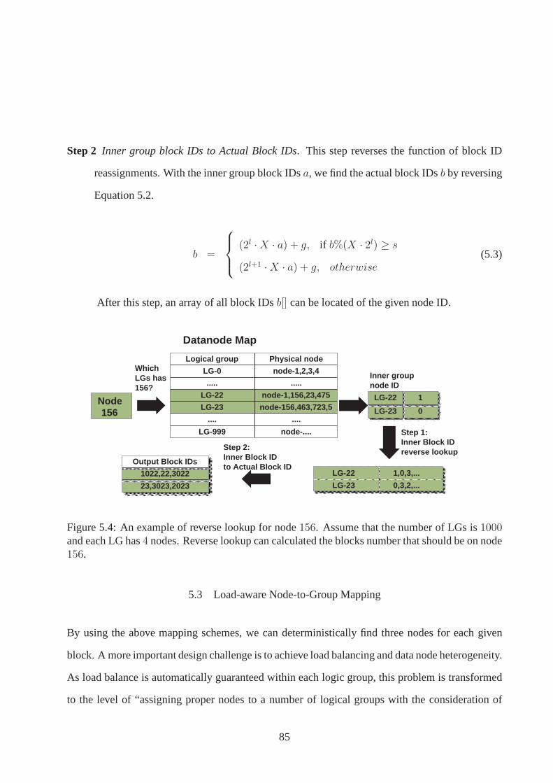
Step 2 Inner group block IDs to Actual Block IDs. This step reverses the function of block ID
reassignments. With the inner group block IDsa, we find the actual block IDsb by reversing
Equation 5.2.
b =
(2l ·X · a) + g, if b%(X · 2l) ≥ s
(2l+1 ·X · a) + g, otherwise(5.3)
After this step, an array of all block IDsb[] can be located of the given node ID.
Node 156
Logical group Physical node
LG-0 node-1,2,3,4
..... .....
LG-22 node-1,156,23,475
LG-23 node-156,463,723,5
.... ....
LG-999 node-....
Datanode Map
Which LGs has 156?
Inner group node ID
LG-22 1
LG-23 0
Step 1: Inner Block ID reverse lookup
LG-22 1,0,3,...
LG-23 0,3,2,...
Step 2: Inner Block ID to Actual Block ID
Output Block IDs
1022,22,3022
23,3023,2023
Figure 5.4: An example of reverse lookup for node156. Assume that the number of LGs is1000and each LG has4 nodes. Reverse lookup can calculated the blocks number thatshould be on node156.
5.3 Load-aware Node-to-Group Mapping
By using the above mapping schemes, we can deterministically find three nodes for each given
block. A more important design challenge is to achieve load balancing and data node heterogeneity.
As load balance is automatically guaranteed within each logic group, this problem is transformed
to the level of “assigning proper nodes to a number of logicalgroups with the consideration of
85

data node capacity and load balancing”. Using our block-to-node mapping, this problem can be
determined by the number of logic groups laid on one data node.
More specifically, we define a factor named “Logic Group Coverage (LGC)” factor to symbolize
the number of groups that resides on one data node. Assume that one data nodej is covered byα
logic groups whereα1 is the number of groups that belongs to[1, s] or (X,X + s]; andα2 is the
number of groups that belongs to(s,X ], the logic group coverage for data nodej is:
covj = (α1/2 + α2)/(X + s) (5.4)
Using this LGC factor, we develop a load-aware policy to assign nodes to logic groups, as shown
in Algorithm 5.3.1. The key idea is to iteratively choose thedata nodes with less LGC factor so
that the number of blocks distributed on this node can be similar with the others.
Algorithm 5.3.1 Pseudocode of load-aware nodes-to-group mappingInput: The cluster hasm number of nodes, each with a LGC factorcov[];Output: Assign thesem nodes toX equal sized logic groups with the consideration of equal distribution on each node.Steps:if cov[] == NULL then
randomly choose one node to put in the first logic groupg[0];end ifRetrieve and sort the LGC factors from all data nodes;put the sorted nodes intocoverageQueue;
int i = 0;//choose the data node for each logic groupgwhile i ≤ X do
if coverageQueue.peek() matches the rack requirementthenselectfitDataNode = coverageQueue.poll() as one member for the groupg[i];updatecoverage for fitDataNode;updatecoverageuQueue;
if g[i] is full theni++; continue; //continue for next group
end ifelse
update coverageQueue;end if
end while
When new nodes are added to the system, we choose to add the number of groups. Originally from
linear hashing, for each newly added group (i.e. groupgnew is added), half of the data from one of
86
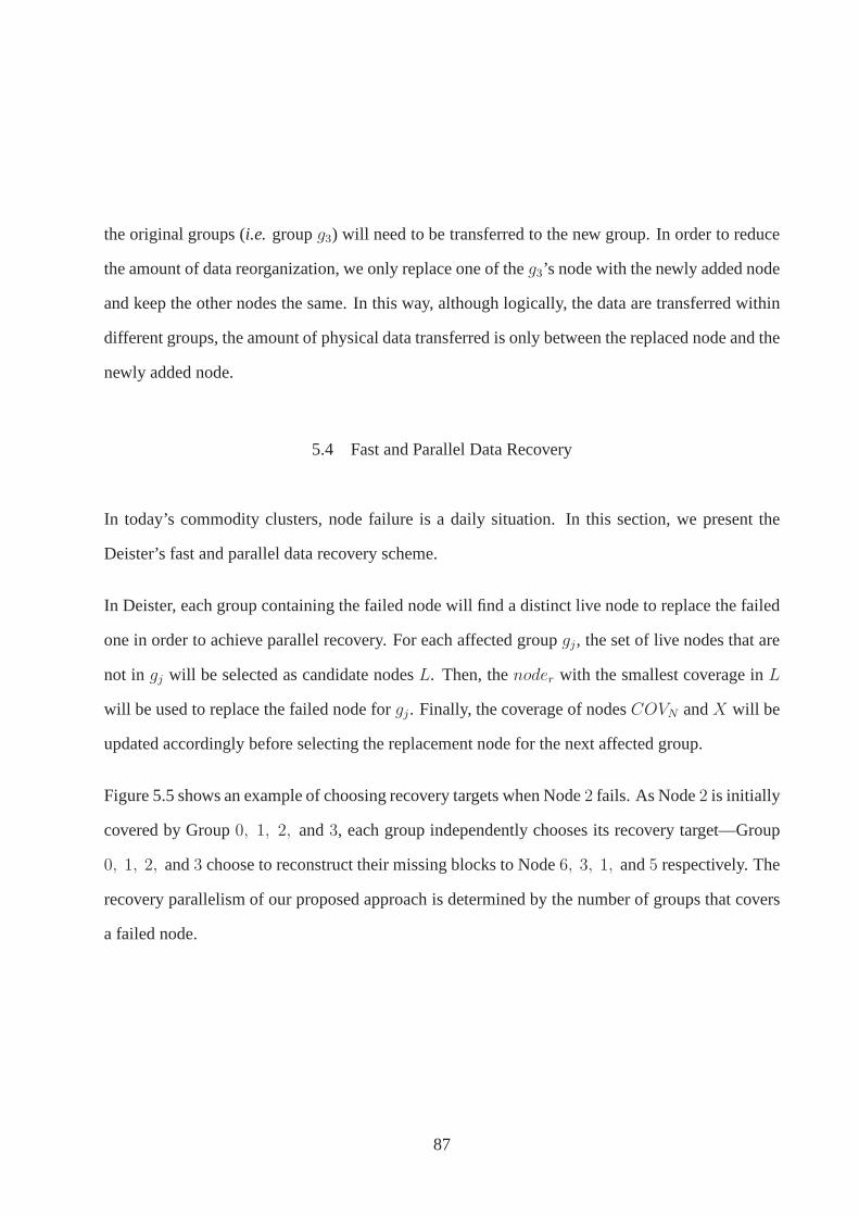
the original groups (i.e. groupg3) will need to be transferred to the new group. In order to reduce
the amount of data reorganization, we only replace one of theg3’s node with the newly added node
and keep the other nodes the same. In this way, although logically, the data are transferred within
different groups, the amount of physical data transferred is only between the replaced node and the
newly added node.
5.4 Fast and Parallel Data Recovery
In today’s commodity clusters, node failure is a daily situation. In this section, we present the
Deister’s fast and parallel data recovery scheme.
In Deister, each group containing the failed node will find a distinct live node to replace the failed
one in order to achieve parallel recovery. For each affectedgroupgj, the set of live nodes that are
not in gj will be selected as candidate nodesL. Then, thenoder with the smallest coverage inL
will be used to replace the failed node forgj. Finally, the coverage of nodesCOVN andX will be
updated accordingly before selecting the replacement nodefor the next affected group.
Figure 5.5 shows an example of choosing recovery targets when Node2 fails. As Node2 is initially
covered by Group0, 1, 2, and3, each group independently chooses its recovery target—Group
0, 1, 2, and3 choose to reconstruct their missing blocks to Node6, 3, 1, and5 respectively. The
recovery parallelism of our proposed approach is determined by the number of groups that covers
a failed node.
87
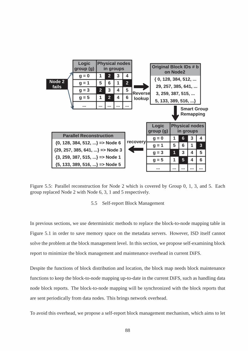
Logic group (g)
Physical nodes in groups
g = 0 1 2 3 4
g = 1 5 6 1 2
g = 3 2 3 4 5
g = 5 1 2 4 6
... ... ... ... ...
Original Block IDs # b on Node 2
{ 0, 128, 384, 512, ...
1 29, 257, 385, 641, ...
3, 259, 387, 515, ...
5, 133, 389, 516, ...}
Node 2 fails
Logic group (g)
Physical nodes in groups
g = 0 1 6 3 4
g = 1 5 6 1 3
g = 3 1 3 4 5
g = 5 1 5 4 6
... ... ... ... ...
Reverse lookup
Parallel Reconstruction
{0, 128, 384, 512, ...} => Node 6
{29, 257, 385, 641, ...} => Node 3
{3, 259, 387, 515, ...} => Node 1
{5, 133, 389, 516, ...} => Node 5
Smart Group Remapping
recovery
Figure 5.5: Parallel reconstruction for Node 2 which is covered by Group 0, 1, 3, and 5. Eachgroup replaced Node 2 with Node 6, 3, 1 and 5 respectively.
5.5 Self-report Block Management
In previous sections, we use deterministic methods to replace the block-to-node mapping table in
Figure 5.1 in order to save memory space on the metadata servers. However, ISD itself cannot
solve the problem at the block management level. In this section, we propose self-examining block
report to minimize the block management and maintenance overhead in current DiFS.
Despite the functions of block distribution and location, the block map needs block maintenance
functions to keep the block-to-node mapping up-to-date in the current DiFS, such as handling data
node block reports. The block-to-node mapping will be synchronized with the block reports that
are sent periodically from data nodes. This brings network overhead.
To avoid this overhead, we propose a self-report block management mechanism, which aims to let
88
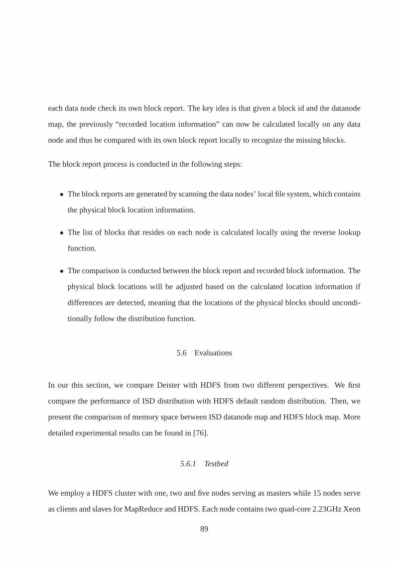
each data node check its own block report. The key idea is thatgiven a block id and the datanode
map, the previously “recorded location information” can now be calculated locally on any data
node and thus be compared with its own block report locally torecognize the missing blocks.
The block report process is conducted in the following steps:
• The block reports are generated by scanning the data nodes’ local file system, which contains
the physical block location information.
• The list of blocks that resides on each node is calculated locally using the reverse lookup
function.
• The comparison is conducted between the block report and recorded block information. The
physical block locations will be adjusted based on the calculated location information if
differences are detected, meaning that the locations of thephysical blocks should uncondi-
tionally follow the distribution function.
5.6 Evaluations
In our this section, we compare Deister with HDFS from two different perspectives. We first
compare the performance of ISD distribution with HDFS default random distribution. Then, we
present the comparison of memory space between ISD datanodemap and HDFS block map. More
detailed experimental results can be found in [76].
5.6.1 Testbed
We employ a HDFS cluster with one, two and five nodes serving asmasters while 15 nodes serve
as clients and slaves for MapReduce and HDFS. Each node contains two quad-core 2.23GHz Xeon
89
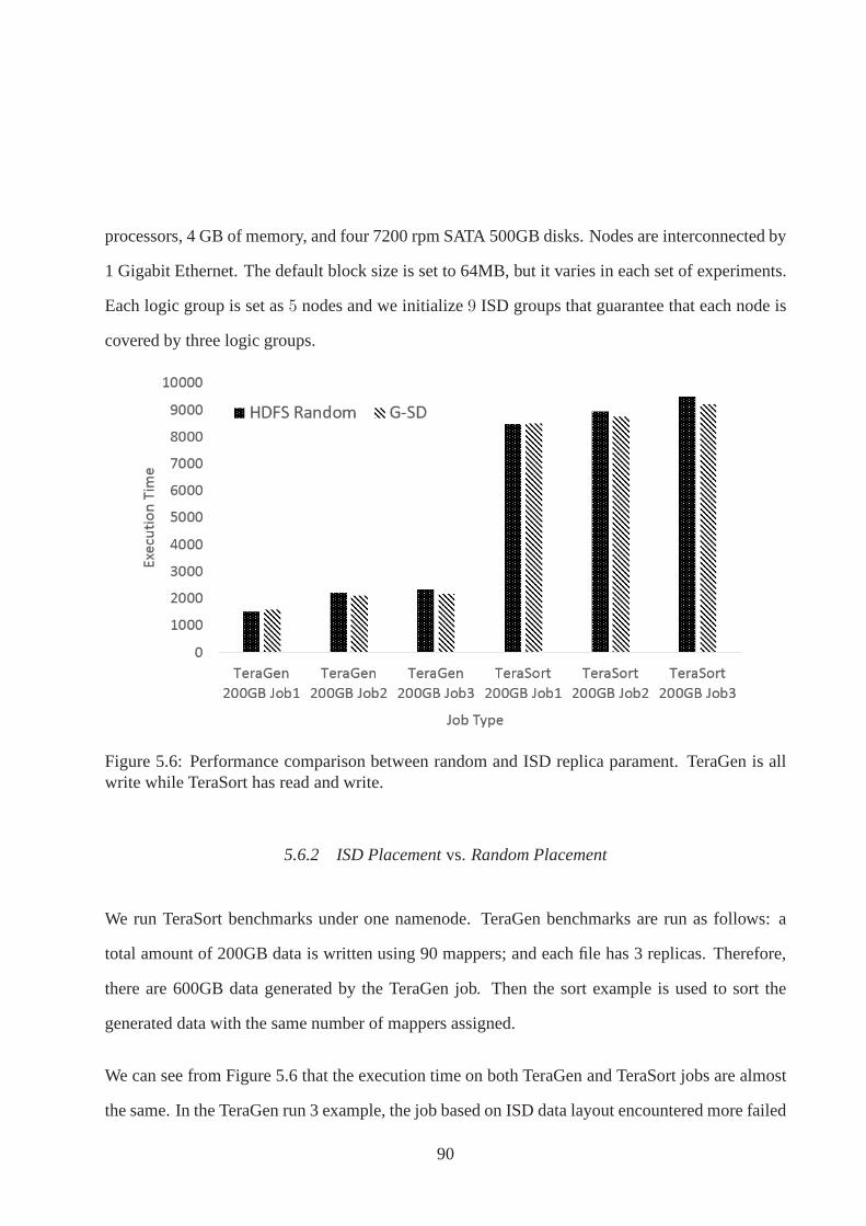
processors, 4 GB of memory, and four 7200 rpm SATA 500GB disks. Nodes are interconnected by
1 Gigabit Ethernet. The default block size is set to 64MB, butit varies in each set of experiments.
Each logic group is set as5 nodes and we initialize9 ISD groups that guarantee that each node is
covered by three logic groups.
Figure 5.6: Performance comparison between random and ISD replica parament. TeraGen is allwrite while TeraSort has read and write.
5.6.2 ISD Placementvs. Random Placement
We run TeraSort benchmarks under one namenode. TeraGen benchmarks are run as follows: a
total amount of 200GB data is written using 90 mappers; and each file has 3 replicas. Therefore,
there are 600GB data generated by the TeraGen job. Then the sort example is used to sort the
generated data with the same number of mappers assigned.
We can see from Figure 5.6 that the execution time on both TeraGen and TeraSort jobs are almost
the same. In the TeraGen run 3 example, the job based on ISD data layout encountered more failed
90
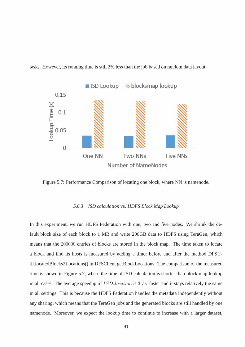
tasks. However, its running time is still 2% less than the jobbased on random data layout.
Figure 5.7: Performance Comparison of locating one block, where NN is namenode.
5.6.3 ISD calculationvs. HDFS Block Map Lookup
In this experiment, we run HDFS Federation with one, two and five nodes. We shrink the de-
fault block size of each block to 1 MB and write 200GB data to HDFS using TeraGen, which
means that the200000 entries of blocks are stored in the block map. The time taken to locate
a block and find its hosts is measured by adding a timer before and after the method DFSU-
til.locatedBlocks2Locations() in DFSClient.getBlockLocations. The comparison of the measured
time is shown in Figure 5.7, where the time of ISD calculationis shorter than block map lookup
in all cases. The average speedup ofISD location is 3.7× faster and it stays relatively the same
in all settings. This is because the HDFS Federation handlesthe metadata independently without
any sharing, which means that the TeraGen jobs and the generated blocks are still handled by one
namenode. Moreover, we expect the lookup time to continue toincrease with a larger dataset,
91
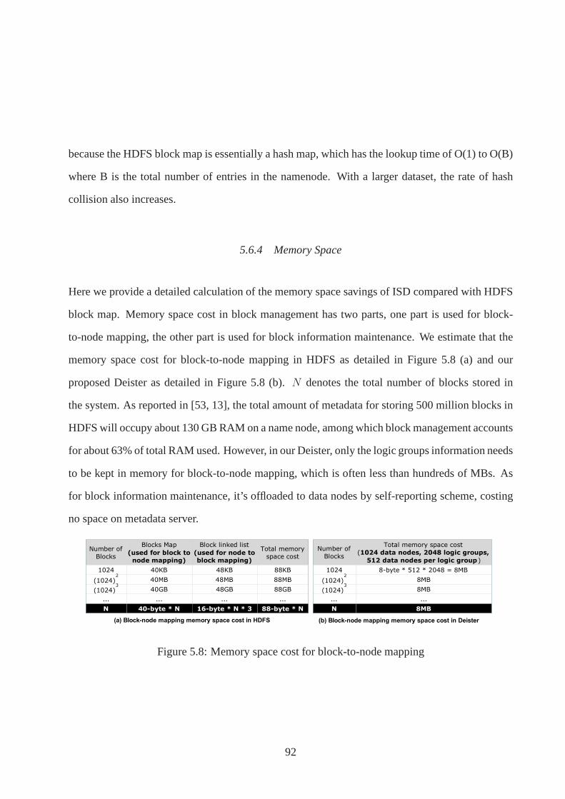
because the HDFS block map is essentially a hash map, which has the lookup time of O(1) to O(B)
where B is the total number of entries in the namenode. With a larger dataset, the rate of hash
collision also increases.
5.6.4 Memory Space
Here we provide a detailed calculation of the memory space savings of ISD compared with HDFS
block map. Memory space cost in block management has two parts, one part is used for block-
to-node mapping, the other part is used for block information maintenance. We estimate that the
memory space cost for block-to-node mapping in HDFS as detailed in Figure 5.8 (a) and our
proposed Deister as detailed in Figure 5.8 (b).N denotes the total number of blocks stored in
the system. As reported in [53, 13], the total amount of metadata for storing 500 million blocks in
HDFS will occupy about 130 GB RAM on a name node, among which block management accounts
for about 63% of total RAM used. However, in our Deister, onlythe logic groups information needs
to be kept in memory for block-to-node mapping, which is often less than hundreds of MBs. As
for block information maintenance, it’s offloaded to data nodes by self-reporting scheme, costing
no space on metadata server.
Number of
Blocks
Blocks Map
(used for block to
node mapping)
Block linked list
(used for node to
block mapping)
Total memory
space cost
1024 40KB 48KB 88KB
(1024)2
40MB 48MB 88MB
(1024)3
40GB 48GB 88GB
... ... ... ...
N 40-byte * N 16-byte * N * 3 88-byte * N
Number of
Blocks
Total memory space cost
(1024 data nodes, 2048 logic groups,
512 data nodes per logic group )
1024 8-byte * 512 * 2048 = 8MB
(1024)2
8MB
(1024)3
8MB
... ...
N 8MB
(a) Block-node mapping memory space cost in HDFS (b) Block-node mapping memory space cost in Deister
Figure 5.8: Memory space cost for block-to-node mapping
92
CHAPTER 6: CONCLUSION
In this section, we present concluding remarks of the proposed designs.
Firstly, we have proposed a Group-shifted declustering layout, which can be used in the large
file system and support a fast and efficient reverse lookup scheme. We have summarized the
importance of the reverse lookup problem, which were overlooked in previous researches. We
also examined the current reverse lookup solutions, presented their limitations and proposed a
scalable reverse lookup scheme. G-SD extends our previous work shifted declustering so that this
multi-way replication-based data layout can be adapted in large file systems. According to the
comprehensive mathematical proofs and availability analysis, G-SD is scalable and can largely
reduce the data reorganization overhead of SD when node joining. Moreover, by comparing with
the traditional reverse lookup method including centralized and decentralized metadata traversing,
we conducted real-life experiments to show that the G-SD RL effectively reduced the reverse
lookup response time by more than three orders of magnitude times faster.
Secondly, we have proposed “PERP” which minimizes the energy consumption while satisfying
the performance and recovery constraints and outputs the provisioning of proper active node num-
ber and recovery speed. The model is motivated by taking recovery process into consideration of
the current power-efficiency storage because the degradation mode is becoming an non-neglectable
operational state, which is overlooked by previous researches. We summarize the preconditions
of deriving PERP results and study the applicability of working with current data layouts. Group-
rotational declustering layout is studied as an example of how to choose the proper nodes to open.
According to comprehensive experiments on our CASS clusterwith 24 nodes, we first prove the
optimality by comparing PERP with various configurations based on the original output. More-
over, experiments of comparing PERP with the maximum recovery policy indicate that with both
93

satisfying performance and recovery constraints, our solution saves up to 25% of energy.
Finally, we are developed a light-weight block management scheme Deister, which uses ISD, a
deterministic declustering block distribution method to scale-up each metadata server by reducing
the memory space overhead and offloading the block report handling to the data nodes. Our exper-
iments and calculations show that the I/O speed of the ISD placement is comparable with HDFS
random placement. The calculation shows that 63% memory space can be saved by ISD in a 1024
node and 500 million blocks.
94

APPENDIX : PROOF OF REORGANIZATION OVERHEAD
95

In Section 3, we explicitly present the overhead of adding nodes in an already balanced group.
Here we give the proof that how many objects are moved from theoriginal disk to another one.
The addition process could be divided into four scenarios, as shown follows.
Case 1: α is odd,β is even.
In this case, the added group will still have an odd (α + β) number of storage nodes which will
not generate “bubbles” as the case of even number nodes do. Soall added nodes are required to
fulfilled with the objects.
PROOF. According to the shifted declustering layout, the layout scenario after addition process is
as follows.
q1 = (α + β − 1)/2 (.1)
z1 = ⌊a/(α + β)⌋ (.2)
y1 = (z1%q1) + 1 (.3)
disk(a, i)1 = (a+ iy)%(α + β) (.4)
In order to calculate the objects moved, we will comparedisk(a, i) (before addition) anddisk(a, i)1
(after addition) whena andi are the same in both case.
1. In the first iteration (z1 = 0, y1 = 1), disk(a, i)1 = (a + i)%(α + β) (after addition) while
disk(a, i) = (a + i)%α (before addition). When(a + i) ≤ α, the objects will not moved.
Whenm < (a + i) ≤ (α + β) the objects will be moved from the following iterations and
three more objects are substituted in the front by the comingobjects.e.g. in Figure 3.1, if
β = 2, redundancy group (9,i) and (10,i)(i = 0, 1 or 2) will be moved to the newly added
nodes and (7,2), (8,1) and (8,2) are moved to the newly added nodes. So the number of
96

moved objects is3 ∗ (β + 1).
2. In the following iterations (z1 ≥ 1,y1 ≥ 1), we can consider it as stuffing empty slots—each
iterations’ firstβ ∗ z slots will be empty because they are moved to the previous iterations.
Moreover, since the total node number is odd and the empty slots’ number are even, there
is no chance fordisk1(a, i) = disk(a, i). So every following objects in this iteration are
needed to move to the previous slots and fill them. In this casethe moved objects are(q −
1)α ∗ 3.
Add up the above results, the total reorganized objects are[(q − 1)α + (β + 1)]× 3. �
Case 2:α is odd,β is odd.
In this case, the group number will change from odd to even, and “bubbles” are added to maintain
the SD layout.
PROOF. After addition, the layout equations are as follows.
q2 = (α + β − 2)/2 (.5)
z2 = ⌊a/α+ β − 2⌋ (.6)
y2 = (z%q′) + 1 (.7)
db2 = (α + β − 1− z)%(m+ l) (.8)
disk(a, 0)2 = a%(α + l) (.9)
disk(a, i)2 =
(a + iy + 1)%(α + β)∗
(a + iy)%(α+ β)∗∗, (i ≥ 1) (.10)
97
*: if one of the following applies:
i) disk(a, 0)2 < db2 anddisk(a, 0) + iy ≥ db2
ii) disk(a, 0)2 > db2 anddisk(a, 0) + iy ≥ db2 + n
***:otherwise
wheredisk(a, i)2 is the disk position for
object (a,i). Then we compare thedisk(a, i) (before) anddisk(a, i)2 (after) to determine how
many objects are needed to be reorganized.
1. In the first iteration (z2 = 0, y2 = 1), disk(a, i)2 = (a + i)%(α + β) and the “bubble”
db2 = (α + β − 1). While the originaldisk(a, i) = (a + i)%α and no “bubble” is in it.
So normally the total number of objects moved are3 ∗ l. Except one case: whenβ = 1,
there is no need to change any object position, so the number of moved objects are 0 as
Equation 3.16∗∗∗ shows.
2. In the following iterations (z2 ≥ 1,y2 ≥ 1), no matterl is one or not, “bubble”s are generated
in each iteration. The firstz column of objects are moving after the “bubble”, which makes
the reorganization process similar as Case 1—all the objects are reorganized to other nodes.
The reorganization overhead is(q − 1)α ∗ 3.
So the total number of reorganized objects is(q − 1)α × 3 whenβ = 1 and[(q − 1)α+ β] × 3
whenβ ≤ 1. �
Case 3:α is even,β is odd. In this case, the group number is becoming to odd (α+β) after addition.
Since there are “bubbles” in the layout before addition, they will be filled out after adding nodes
98

into the group. PROOF. After addition, the layout equationsare as follows.
q3 = (α + β − 1)/2 (.11)
z3 = ⌊a/(α + β)⌋ (.12)
y3 = (z3%q3) + 1 (.13)
disk(a, i)3 = (a+ iy)%(α + β) (.14)
wheredisk(a, i)3 is the disk position for object (a,i). We compare the disk positiondisk(a, i)
(before) anddisk(a, i)3 (after)for the object (a,i).
1. In the first iteration (z3 = 0, y3 = 1), disk(a, i)3 = (a + i)%(α + β) (after addition)
while disk(a, i) = (a + i)%m (before addition) anddb = (α − 1). This means there are
3 ∗ (β + 1) objects from the second iteration as Case 1 did and 3 extra objects to fill the
“bubble”. However, there is one exception: whena = m − 1, disk(a, 0) = α − 1 and
disk(a, 0)3 = α− 1, this object (m-1,0) is moved from second iteration to the first iteration
with a different offset but a same disk. So the total number ofobjects reorganized for the
first iteration is(β + 1) ∗ 3 + 2
2. In the following iterations (z3 ≥ 1,y3 ≥ 1), disk(a, i)3 = (a+ iy3)%(α+β) (after addition)
whiledisk(a, i) = (a+ iy)%mor (a+ iy+1)%m (before addition). The situation is similar
to Case 1, all objects are needed to be reorganized to a different disk location.
So the total number of reorganized objects is[(q − 1)α+ (β + 1)]× 3 + 2. �
Case 4:m is even,l is even. In this case, the group will still have even (m + 2) number of nodes.
Adding nodes will not result in the fulfillment of the “bubbles”. PROOF. After addition, the layout
99

equations are as follows.
q4 = (α + β − 2)/2 (.15)
z4 = ⌊a/α+ β − 2⌋ (.16)
y4 = (z%q′) + 1 (.17)
db4 = (α + β − 1− z)%(α + β) (.18)
disk(a, 0)4 = a%(α + β) (.19)
disk(a, i)4 =
(a + iy + 1)%(α + β)∗
(a + iy)%(α+ β)∗∗, (i ≥ 1) (.20)
*: if one of the following applies:
i) disk4(a, 0) < db4 anddisk(a, 0) + iy ≥ db4
ii) disk4(a, 0) > db4 anddisk(a, 0) + iy ≥ db4 + α
**:otherwise
wheredisk(a, i)2 is the disk position for
object (a,i). Then we compare thedisk(a, i) (before addition) anddisk(a, i)4 (after addition) to
determine how many objects are needed to be reorganized.
1. In the first iteration (z4 = 0, y4 = 1), disk(a, i)4 = (a + i)%(α + β) and the “bubble”
db4 = α + β − 1. While the originaldisk(a, i) = (a + i)%(α − 1) and the “bubble”
db = α − 1. So the total number of objects moved are3 ∗ (β + 1). Also, we have to the
similar exception as the one in Case 3 Proof 1): whena = α− 1, disk(a, 0) = disk(a, 0)4.
So the number of moved objects3 ∗ β + 2.
2. In the following iterations (z2 ≥ 1,y2 ≥ 1), the reorganization process is similar to Case 1—
all the objects are reorganized to other nodes. The reorganization overhead is(q − 1)α ∗ 3.
So the total number of reorganized objects is[(q − 1)α+ β]× 3 + 2 �
100
LIST OF REFERENCES
[1] An Introduction to HDFS Federation. http://hortonworks.com/blog/an-introduction-to-hdfs-
federation/.
[2] Big data analytics. http://www.sas.com/offices/europe/uk/downloads/bigdata/eskills/eskills.pdf.
[3] Cloud storage for the modern data center—an introduction to gluster architecture.
http://moo.nac.uci.edu/ hjm/fs/AnIntroductionTo GlusterArchitectureV7110708.pdf.
[4] Earth surface and interior. http://science.nasa.gov/earth-science/focus-areas/surface-and-
interior/.
[5] Facebook. http://www.facebook.com/.
[6] Jensen’s inequality. http://en.wikipedia.org/wiki/Jenseninequality.
[7] Marmot nodes. https://www.nmc-probe.org/wiki/Marmot:Nodes.
[8] The Pigeon Hole Principle. http://zimmer.csufresno.edu/larryc/proofs/proofs.pigeonhole.html.
[9] The principle of weakest link. http://consciousconversation.com/Essays/
ThePrincipleoftheWeakestLink.htm.
[10] Remotefs. http://remotefs.sourceforge.net/.
[11] Service-level agreement. http://en.wikipedia.org/wiki/Service-levelagreement.
[12] The sloan digital sky survey. http://www.sdss.org/.
[13] Standalone block management for hdfs namenode. https://issues.apache.org/jira/secure/
attachment/12618294/Proposal.pdf.
101
[14] Umass trace repository. http://traces.cs.umass.edu/index.php/Storage/Storage.
[15] Hrishikesh Amur, James Cipar, Varun Gupta, Gregory R. Ganger, Michael A. Kozuch, and
Karsten Schwan. Robust and flexible power-proportional storage. InProceedings of the
1st ACM symposium on Cloud computing, SoCC ’10, pages 217–228, New York, NY, USA,
2010. ACM.
[16] Ryan Stutsman Sachin Katti John Ousterhout Asaf Cidon,Stephen Rumble and Mendel
Rosenblum. Copysets: Reducing the frequency of data loss incloud storage. InUNENIX
Annual Technical Conference. USENIX, 2013.
[17] Luiz Andre Barroso and Urs Holzle. The case for energy-proportional computing.Computer,
40:33–37, December 2007.
[18] Dhruba Borthakur. The Hadoop Distributed File System: Architecture and Design. The
Apache Software Foundation, 2007.
[19] P. J. Braam and Others. The Lustre storage architecture. White Paper, Cluster File Systems,
Inc., Oct, 23, 2003.
[20] A. Brinkmann, S. Effert, and F. Meyer auf der Heide. Dynamic and redundant data place-
ment. InProceedings of the 27th International Conference on Distributed Computing Sys-
tems, ICDCS ’07, pages 29–, Washington, DC, USA, 2007. IEEE Computer Society.
[21] Ming-Syan Chen, Hui-I Hsiao, Chung-Sheng Li, and Philip S. Yu. Using rotational mir-
rored declustering for replica placement in a disk-array-based video server.Multimedia Syst.,
5(6):371–379, 1997.
[22] Shenze Chen and Don Towsley. A performance evaluation of RAID architectures. IEEE
Trans. Comput., 45(10):1116–1130, 1996.
102

[23] Dennis Colarelli and Dirk Grunwald. Massive arrays of idle disks for storage archives. In
Proceedings of the 2002 ACM/IEEE conference on Supercomputing, Supercomputing ’02,
pages 1–11, Los Alamitos, CA, USA, 2002. IEEE Computer Society Press.
[24] Peter F. Corbett and Dror G. Feitelson. The Vesta parallel file system.ACM Trans. Comput.
Syst., 14(3):225–264, 1996.
[25] Frank Dabek, M. Frans Kaashoek, David Karger, Robert Morris, and Ion Stoica. Wide-area
cooperative storage with cfs. InProceedings of the Eighteenth ACM Symposium on Operating
Systems Principles, SOSP ’01, pages 202–215, New York, NY, USA, 2001. ACM.
[26] Giuseppe DeCandia, Deniz Hastorun, Madan Jampani, Gunavardhan Kakulapati, Avinash
Lakshman, Alex Pilchin, Swaminathan Sivasubramanian, Peter Vosshall, and Werner Vogels.
Dynamo: amazon’s highly available key-value store. InSOSP ’07: Proceedings of twenty-
first ACM SIGOPS symposium on Operating systems principles, pages 205–220, New York,
NY, USA, 2007. ACM.
[27] Ronald Fagin, Jurg Nievergelt, Nicholas Pippenger, and H. Raymond Strong. Extendible
hashing—a fast access method for dynamic files.ACM Trans. Database Syst.,
4(3):315–344, September 1979.
[28] S. Gurumurthi, A. Sivasubramaniam, M. Kandemir, and H.Franke. Drpm: dynamic speed
control for power management in server class disks. InComputer Architecture, 2003. Pro-
ceedings. 30th Annual International Symposium on, pages 169 – 179, june 2003.
[29] R.J. Honicky and E.L. Miller. Replication under scalable hashing: a family of algorithms for
scalable decentralized data distribution.In Proceedings of 18th International Parallel and
Distributed Processing Symposium, 2004., page 96, 26-30 April 2004.
103
[30] Hui-I Hsiao and David J. DeWitt. Chained declustering:A new availability strategy for
multiprocessor database machines. InProceedings of the Sixth International Conference on
Data Engineering, pages 456–465, Washington, DC, USA, 1990. IEEE Computer Society.
[31] Yu Hua, Yifeng Zhu, Hong Jiang, Dan Feng, and Lei Tian. Supporting scalable and adaptive
metadata management in ultra large-scale file systems.IEEE Transactions on Parallel and
Distributed Systems, 99(PrePrints), 2010.
[32] David Karger, Eric Lehman, Tom Leighton, Mathhew Levine, Daniel Lewin, and Rina Pan-
igrahy. Consistent hashing and random trees: Distributed caching protocols for relieving
hot spots on the world wide web. InIn ACM Symposium on Theory of Computing, pages
654–663, 1997.
[33] David Karger, Eric Lehman, Tom Leighton, Rina Panigrahy, Matthew Levine, and Daniel
Lewin. Consistent hashing and random trees: Distributed caching protocols for relieving hot
spots on the world wide web. InProceedings of the Twenty-ninth Annual ACM Symposium
on Theory of Computing, STOC ’97, pages 654–663, New York, NY, USA, 1997. ACM.
[34] Jonathan Koomey. Growth in data center electricity use2005 to 2010.Oakland, CA: Analyt-
ics Press. August, 1:2010, 2011.
[35] John Kubiatowicz, David Bindel, Yan Chen, Steven Czerwinski, Patrick Eaton, Dennis Geels,
Ramakrishan Gummadi, Sean Rhea, Hakim Weatherspoon, Westley Weimer, Chris Wells,
and Ben Zhao. Oceanstore: an architecture for global-scalepersistent storage.SIGPLAN
Not., 35(11):190–201, 2000.
[36] 2010 L.A. Barroso, ACM SIGMOD. Keynote: Warehouse-scale computing.
104
[37] Dong Li and Jun Wang. Eeraid: energy efficient redundantand inexpensive disk array. In
Proceedings of the 11th workshop on ACM SIGOPS European workshop, EW 11, New York,
NY, USA, 2004. ACM.
[38] Minghong Lin, A. Wierman, L.L.H. Andrew, and E. Thereska. Dynamic right-sizing for
power-proportional data centers. InINFOCOM, 2011 Proceedings IEEE, pages 1098 –1106,
april 2011.
[39] W. Litwin and T. Risch. LH*g: a high-availability scalable distributed data structure by
record grouping.Knowledge and Data Engineering, IEEE Transactions on, 14(4):923 –927,
jul. 2002.
[40] Witold Litwin. Linear hashing: A new tool for file and table addressing. InProceedings of
the Sixth International Conference on Very Large Data Bases- Volume 6, VLDB ’80, pages
212–223. VLDB Endowment, 1980.
[41] Witold Litwin, Marie-Anna Neimat, and Donovan A Schneider. Lh*—a scalable, distributed
data structure.ACM Trans. Database Syst., 21(4):480–525, 1996.
[42] Witold Litwin, Marie-Anne Neimat, and Donovan A. Schneider. RP*: A family of order
preserving scalable distributed data structures. InVLDB, pages 342–353, 1994.
[43] Zhenhua Liu, Minghong Lin, Adam Wierman, Steven H. Low,and Lachlan L.H. Andrew.
Greening geographical load balancing.SIGMETRICS Perform. Eval. Rev., 39:193–204, June
2011.
[44] Petar Maymounkov and David Mazieres. Kademlia: A peer-to-peer information system based
on the xor metric. InRevised Papers from the First International Workshop on Peer-to-Peer
Systems, IPTPS ’01, pages 53–65, London, UK, UK, 2002. Springer-Verlag.
105

[45] Michael Ovsiannikov, Silvius Rus, Damian Reeves, PaulSutter, Sriram Rao, and Jim Kelly.
The quantcast file system.Proc. VLDB Endow., 6(11):1092–1101, August 2013.
[46] Eduardo Pinheiro and Ricardo Bianchini. Energy conservation techniques for disk array-
based servers. InProceedings of the 18th annual international conference onSupercomput-
ing, ICS ’04, pages 68–78, New York, NY, USA, 2004. ACM.
[47] Eduardo Pinheiro, Ricardo Bianchini, and Cezary Dubnicki. Exploiting redundancy to
conserve energy in storage systems. InProceedings of the Joint International Conference
on Measurement and Modeling of Computer Systems, SIGMETRICS ’06/Performance ’06,
pages 15–26, New York, NY, USA, 2006. ACM.
[48] Eduardo Pinheiro, Wolf-Dietrich Weber, and Luiz Andr´e Barroso. Failure trends in a large
disk drive population. InProceedings of the 5th USENIX Conference on File and Storage
Technologies, FAST ’07, pages 2–2, Berkeley, CA, USA, 2007. USENIX Association.
[49] Shun-Tak Leung Sanjay Ghemawat, Howard Gobioff. The google file system.OPERATING
SYSTEMS REVIEW, 37:29–43, 2003.
[50] Bianca Schroeder and Garth A. Gibson. Disk failures in the real world: What does an mttf
of 1,000,000 hours mean to you? InProceedings of the 5th USENIX Conference on File and
Storage Technologies, FAST ’07, 2007.
[51] Bianca Schroeder and Garth A. Gibson. Understanding disk failure rates: What does an mttf
of 1,000,000 hours mean to you?ACM Trans. Storage, 3(3), October 2007.
[52] Penju Shang, Jun Wang, Huijun Zhu, and Peng Gu. A new placement-ideal layout for multi-
way replication storage system.IEEE Transactions on Computers, 99(PrePrints), 2010.
[53] Konstantin V. Shvachko. HDFS Scalability: The Limits to Growth. login: The Magazine of
USENIX, 35(2):6–16, April 2010.
106
[54] I. Stoica, R. Morris, D. Liben-Nowell, D.R. Karger, M.F. Kaashoek, F. Dabek, and H. Balakr-
ishnan. Chord: a scalable peer-to-peer lookup protocol forinternet applications.Networking,
IEEE/ACM Transactions on, 11(1):17 – 32, feb. 2003.
[55] Adam Sweeney, Adam Sweeney, Doug Doucette, Wei Hu, Curtis Anderson, Mike Nishimoto,
and Geoff Peck. Scalability in the XFS file system. InIn Proceedings of the 1996 USENIX
Annual Technical Conference, pages 1–14, 1996.
[56] Eno Thereska, Austin Donnelly, and Dushyanth Narayanan. Sierra: practical power-
proportionality for data center storage. InProceedings of the sixth conference on Computer
systems, EuroSys ’11, pages 169–182, New York, NY, USA, 2011. ACM.
[57] Peter Vajgel. Needle in a haystack:efficient storage ofbillions of photos.
http://www.facebook.com/note.php?noteid=76191543919, 2009.
[58] Randolph Wang, Olph Y. Wang, and Thomas E. Anderson. xFS: A wide area mass storage
file system. InIn Fourth Workshop on Workstation Operating Systems, pages 71–78, 1993.
[59] Charles Weddle, Mathew Oldham, Jin Qian, An i Andy Wang,and Peter Reiher. Paraid:
The gearshifting power-aware raid. InIn Proc. USENIX Conference on File and Storage
Technologies (FAST07, pages 245–260. USENIX Association, 2007.
[60] Sage Weil, Scott A. Brandt, Ethan L. Miller, Darrell D. E. Long, and Carlos Maltzahn. Ceph:
A scalable, high-pesrformance distributed file system. November 2006.
[61] Sage A. Weil, Scott A. Brandt, Ethan L. Miller, Darrell D. E. Long, and Carlos Maltzahn.
Ceph: A scalable, high-performance distributed file system. In In Proceedings of the 7th
Symposium on Operating Systems Design and Implementation (OSDI, pages 307–320, 2006.
107

[62] Sage A. Weil, Scott A. Brandt, Ethan L. Miller, and Carlos Maltzahn. Crush: controlled,
scalable, decentralized placement of replicated data. InSC ’06: Proceedings of the 2006
ACM/IEEE conference on Supercomputing, page 122, New York, NY, USA, 2006. ACM.
[63] Brent Welch, Marc Unangst, Zainul Abbasi, Garth Gibson, Brian Mueller, Jason Small, Jim
Zelenka, and Bin Zhou. Scalable performance of the panasas parallel file system. InPro-
ceedings of the 6th USENIX Conference on File and Storage Technologies, FAST’08, pages
2:1–2:17, Berkeley, CA, USA, 2008. USENIX Association.
[64] Brian White, Jay Lepreau, Leigh Stoller, Robert Ricci,Shashi Guruprasad, Mac Newbold,
Mike Hibler, Chad Barb, and Abhijeet Joglekar. An integrated experimental environment for
distributed systems and networks. InProceedings of the USENIX Symposium on Operating
System Design and Implementation (OSDI). USENIX, December 2002.
[65] Suzhen Wu, Hong Jiang, Dan Feng, Lei Tian, and Bo Mao. Workout: I/o workload outsourc-
ing for boosting raid reconstruction performance. InProccedings of the 7th conference on
File and storage technologies, pages 239–252, Berkeley, CA, USA, 2009. USENIX Associ-
ation.
[66] Suzhen Wu, Hong Jiang, Dan Feng, Lei Tian, and Bo Mao. Workout: I/o workload outsourc-
ing for boosting raid reconstruction performance. InProccedings of the 7th conference on
File and storage technologies, pages 239–252, Berkeley, CA, USA, 2009. USENIX Associ-
ation.
[67] Tao Xie and Yao Sun. Understanding the relationship between energy conservation and reli-
ability in parallel disk arrays.J. Parallel Distrib. Comput., 71:198–210, February 2011.
[68] Qin Xin, Ethan L. Miller, Thomas Schwarz, Darrell D. E. Long, Scott A. Brandt, and Witold
Litwin. Reliability mechanisms for very large storage systems. pages 146–156, April 2003.
108
[69] Qin Xin, Ethan L. Miller, Thomas Schwarz, Darrell D. E. Long, Scott A. Brandt, and Witold
Litwin. Reliability mechanisms for very large storage systems. pages 146–156, April 2003.
[70] Qin Xin, Thomas J. E. Schwarz, and Ethan L. Miller. Disk infant mortality in large storage
systems. InIn Proc of MASCOTS ?5, pages 125–134, 2005.
[71] Junyao Zhang. Researches on Reverse Lookup problem in Distributed File System. Master’s
thesis, University of Central Florida, USA, 2010.
[72] Junyao Zhang, Pengju Shang, and Jun Wang. A scalable reverse lookup scheme using group-
based shifted declustering layout. InProceedings of the 2011 IEEE International Parallel
& Distributed Processing Symposium, IPDPS ’11, pages 604–615, Washington, DC, USA,
2011. IEEE Computer Society.
[73] Junyao Zhang, Qingdong Wang, Jiangling Yin, Jian Zhou,and Jun Wang. Perp: Attacking
the balance among energy, performance and recovery in storage systems.Journal of Parallel
and Distributed Computing, 2014.
[74] Junyao Zhang, Jiangling Yin, Jun Wang, and Jian Zhou. Onbalance among energy, per-
formance and recovery in storage systems. InDistributed Computing Systems Workshops
(ICDCSW), 2014 IEEE 34th International Conference on, pages 106–112. IEEE, 2014.
[75] Xuechen Zhang, Yuhai Xu, and Song Jiang. Youchoose: A performance interface enabling
convenient and efficient qos support for consolidated storage systems. InMass Storage Sys-
tems and Technologies (MSST), 2011 IEEE 27th Symposium on, pages 1 –12, May 2011.
[76] Xuhong Zhang, Junyao Zhang, Jiangling Yin, Wang Ruijun, Dan Huang, and Jun Wang.
Deister: A light-weight autonomous block management in data-intensive file systems using
deterministic declustering distribution. Insubmitted to Proceedings of the 2015 ACM/IEEE
conference on Supercomputing, SC’15, Austin, TX, USA, 2015. IEEE Computer Society.
109
[77] Huijun Zhu, Peng Gu, and Jun Wang. Shifted declustering: a placement-ideal layout scheme
for multi-way replication storage architecture. InICS ’08: Proceedings of the 22nd annual
international conference on Supercomputing, pages 134–144, New York, NY, USA, 2008.
ACM.
[78] Qingbo Zhu, Francis M. David, Christo F. Devaraj, Zhenmin Li, Yuanyuan Zhou, and Pei
Cao. Reducing energy consumption of disk storage using power-aware cache management.
In Proceedings of the 10th International Symposium on High Performance Computer Archi-
tecture, HPCA ’04, pages 118–129, Washington, DC, USA, 2004. IEEE Computer Society.
[79] Yifeng Zhu, Hong Jiang, Jun Wang, and Feng Xian. HBA: Distributed metadata management
for large cluster-based storage systems.Parallel and Distributed Systems, IEEE Transactions
on, 19(6):750 –763, june 2008.
110