Embed Size (px)
Citation preview
Research Experience for Undergraduates Program
Research Reports
Indiana University, Bloomington
Summer 2016
Contents
Geometry of Hyperbolic Percolation Clusters . . . . . . . . . . . . 5Emma Brissett
Searching for Solitary Pseudo-Anosovs . . . . . . . . . . . . . . . . 16Yvonne Chazal
Klein Bottle Constructions . . . . . . . . . . . . . . . . . . . . . . . . 39James Dix
On Surfaces that are Intrinsically Surfaces of Revolution . . . . . 44Daniel Freese
Some Results in the Theory of Elastic Networks . . . . . . . . . . 74Bat Dejean and Christian Gorski
GTR+Γ+I Model Identifiability using a Discrete Gamma Dis-tribultion . . . . . . . . . . . . . . . . . . . . . . . . . . . . . . . . . 109Kees McGahan
1

Preface
During the summer of 2016 five students participated in the Undergraduate Re-search Experience program in Mathematics at Indiana University. This programwas sponsored by Indiana University and the Department of Mathematics. Theprogram ran for eight weeks, from June 6 through July 31, 2016. Five facultyserved as research advisers to the students from Indiana University:
• Chris Connell worked with Emma Brissett.
• Elizabeth Housworth worked with Kees McGahan.
• Chris Judge worked with Yvonne Chazal.
• Jeffrey Meier worked with James Dix.
• Dylan Thurston worked with Baptiste Dejean, Christian Gorski and EmilyTumber.
• Matthias Weber worked with Daniel Freese.
Following the introductory pizza party, students began meeting with theirfaculty mentors and continued to do so throughout the next eight weeks. Thestudents also participated in a number of social events and educational oppor-tunities and field trips.
Individual faculty gave talks throughout the program on their research,about two a week. Students also received LaTeX training in a series of work-shops. Other opportunities included the option to participate in a GRE andsubject test preparation seminar. Additional educational activities includedtours of the library, the Slocum puzzle collection at the Lilly Library and the IUcyclotron facility, and self guided tours of the art museum. Students presentedtheir work to faculty mentors and their peers at various times. This culmi-nated in their presentations both in poster form and in talks at the statewideIndiana Summer Undergraduate Research conference which we hosted at theBloomington campus of IU.
On the lighter side, students were treated to a reception by the graduateschool as well as the opportunity to a fun filled trip to a local amusement park.They were also given the opportunity to enjoy a night of “laser tag” courtesyof the Department of Mathematics.
2
The summer REU program required the help and support of many differentgroups and individuals to make it a success. We foremost thank the IndianaUniversity and the Department of Mathematics for major financial support forthis bridge year between two National Science Foundation grants. We especiallythank our staff member Mandie McCarty for coordinating the complex logisti-cal arrangments (housing, paychecks, information packets, meal plans, frequentshopping for snacks). Additional logistical support was provided by the Depart-ment of Mathematics and our chair, Elizabeth Housworth. We are in particularthankful to Jeff Taylor for the computer support he provided. Thanks to thosefaculty who served as mentors and those who gave lectures. Thanks to DavidBaxter of the Center for Exploration of Energy and Matter (nee IU cyclotron fa-cility) for his personal tour of the LENS facility and lecture. Thanks to AndrewRhoda for his tour of the Slocum Puzzle Collection.
Chris ConnellSeptember, 2016
3

Figure 1: REU Participants, from left to right: Kees McGahan, Emma Brissett,Daniel Freese, Yvonne Chazal, Bat DeJean, James Dix, Christian Gorski.
4

Geometry of Hyperbolic Percolation Clusters
Emma BrissettAdvisor: Chris Connell
September 14, 2016
Abstract
Given an infinite connected graph G, we can perform a Bernoulli bondpercolation on G in the following way: for each edge in G, with probabilityp, the edge remains, and with probability 1 − p, the edge is removed. Weare left with a random subgraph of G containing a combination of finiteand infinite components called clusters. Every infinite connected graphhas constants pc and pu in [0, 1] which are threshold probability valueswith respect to the number of infinite clusters in the percolation subgraph.Of special interest are percolations on hyperbolic graphs. There are manyresults concerning the number of infinite clusters in percolation subgraphsof planar hyperbolic graphs, as well as pc and pu values for such graphs,and we extend these to include nonplanar hyperbolic graphs. From there,we study the asymptotic behavior of infinite clusters in percolations onGromov hyperbolic graphs. Finally, we calculate pc bounds for radiallyhomogeneous graphs.
1 Introduction
An invariant percolation on a graph G is a probability measure on the space ofsubgraphs of G, which is invariant under the automorphisms of G. The con-nected components of an invariant percolation are called clusters. This reportwill focus on Bernoulli(p) bond percolation, which is the random subgraph of Gwhere all vertices V (G) are included and each edge is in the subgraph with prob-ability p, independently. Let pc = pc(G) be the infimum of the set of p ∈ [0, 1]such that the Bernoulli(p) percolation on G has an infinite cluster a.s. We callpc the critical parameter. Likewise, let pu = pu(G) be the infimum of the setof p ∈ [0, 1] such that the Bernoulli(p) percolation on G has a unique infinitecluster a.s.
Let Aut(G) be the group of automorphisms of G. G is transitive if Aut(G) actstransitively on the vertices V (G). G is quasi-transitive if the action of Aut(G)on V (G) has finitely many orbits. G is unimodular if Aut(G) is unimodular,meaning the left-invariant Haar measure is also right-invariant. G has one end iffor every finite set of vertices V0 ∈ V (G), there is exactly one infinite connected
5
component of G/V0. G is discrete if Aut(G) is discrete. Note that discretegraphs are unimodular. G is amenable if there exists a sequence of sets Fn ⊂ Gsuch that
limn→∞
|∂Fn||Fn|
= 0.
G is a nonelementary hyperbolic graph if there is an infinite number of points inthe ideal boundary ∂∞G. Note that transitive, nonelementary, discrete, hyper-bolic graphs are nonamenable. Without transitivity, a nonelementary, discrete,hyperbolic graph could be made amenable by attaching an amenable graph toa vertex. Of particular interest are nonelementary, discrete, Gromov hyperbolicgraphs. G is Gromov hyperbolic if all triangles in G are δ-thin. We call a triangleδ-thin if there exists a δ > 0 such that each side lies in the δ-thickening of theother two sides. For a Gromov hyperbolic graph containing points x, y and z,we define the Gromov product of y and z as follows:
(y, z)x =1
2(d(x, y) + d(x, z)− d(y, z)).
As an introduction to our project, we will examine Bernoulli percolation in thetree case and demonstrate our methods for finding pc and pu for T4.
2 Percolation on T4
T4 is the 4-regular tree and the Cayley graph of the free group on two genera-tors. Like the graphs we will study, T4 is transitive, unimodular, nonamenable,and Gromov-hyperbolic. One key difference is T4 has infinite ends, while thegraphs we will study have one end.
Let ω be the Bernoulli bond percolation on T4 and let S(x, n) be the sphere withcenter x and radius n. We know the probability of not reaching S(x, 1) is theprobability that all four edges are removed: (1− p)4. Therefore, the probabilityof reaching S(x, 1) is 1 − (1 − p)4. The expected number of vertices reachedin S(x, 1) is 4p. For example, if p = 2
3 , we expect that 4(
23
)= 8
3 vertices arereached.
Given that we reached 4p vertices in S(x, 1), the probability of reaching S(x, 2)is 4p(1− (1− p)3), since each vertex in S(x, 1) has three outward edges. Then,the expected number of vertices reached in S(x, 2) is 4p(3p). Continuing on,each vertex will always have three outward edges, so, given that we reachedS(x, n − 1), the expected number of vertices reached in S(x, n) is 4p(3p)n−1.Let Zn be the expected number of vertices reached in S(x, n). Then, pc = 1
3 ,since for p < 1
3 , as n→∞, Zn → 0, and for p > 13 , as n→∞, Zn →∞.
Lemma 1. If G is a transitive graph with more than one end, then pu(G) = 1.
Proof. Suppose for pu < p < 1 there is a unique infinite cluster C ∈ G. Bytransitivity, a sequence in C would be equally likely to occur in any end, so
6
since C is unique, it must have multiple ends. However, by the definition ofends, there exists a finite subgraph T ∈ G such that G/T has disconnectedends. Since p < 1, there is a positive probability that T will be removed, whichcontradicts the assumption that C has multiple ends, so pu = 1.
Since T4 is transitive and has an infinite number of ends, pu(T4) = 1. That is,T4 only has a unique infinite cluster when no edges are removed.
Note that calculating conditional expectation in the tree case is simple, sincethere are single inward edges and a constant number of outward edges. Some ofthe graphs we will study include multiple inward and lateral edges, which makeexpectation calculations more difficult. First, however, we will extend severaltheorems from [3] to include nonplanar graphs.
3 The Number of Infinite Clusters
The following theorem and proof follow results from Theorem 3.3 in [5].
Theorem 2. Each rotation system P on a locally finite graph G determines acellular embedding of G into some oriented surface S such that: i) the 2-cellsare in a bijective correspondence with cycles of P−1r and ii) the rotation systemof this embedding is equal to P .
In other words, every graph G of finite degree embeds in a surface such thatits cycles surround a disk. Let K(G) be the 2-skeleton of G for such an embed-ding. Then, every edge bounds exactly two faces, and we can define the dualG† as follows: let every vertex v† of G† lie in the corresponding face of K(G)and every edge e ∈ E(G) intersect only the dual edge e† ∈ E(G†), and only inone point. Such a dual graph will maintain the properties necessary to extendseveral theorems from [3] to nonplanar graphs.
The following theorem and proof follow results from Theorem 1 in [6].
Theorem 3. For the random variable N0 denoting the number of infinite com-ponents in a percolation, a.s. N0 = 0, 1, or ∞.
Proof. Let Ω be a configuration space 0, 1G, P be a translation ergodic prob-ability measure on Ω, and ω be a configuration in Ω. The random variable N0
and the events N0 = k are invariant under any shift Tj ; therefore by ergdoc-ity there is some k0 = 0, 1, 2, . . . , or ∞ such that P (N0 = k0) = 1. Supposek0 6= 0, 1, or ∞; we wish to obtain a contradiction. Let Wn be the event thatN0 = k0 and each one of the k0 infinite clusters has nonzero intersection with theball B(1, n); then P (Wn) → P (N0 = k0) = 1 and so for some m, P (Wm) > 0.
7
Let V = B(1,m) and define Ψ : Ω→ Ω by
(Ψω)v =
1, v ∈ B(1,m)
wv, v 6∈ B(1,m)
So, Ψ is the transformation which makes all sites in B(1,m) occupied andleaves all other sites unchanged. By Proposition 9, P (Ψ(Wm)) > 0, but clearlyΨ(Wm) ⊂ N0 = 1, thus P (N0 = 1) > 0, which contradicts the suppositionthat k0 6= 0, 1, or ∞.
Let ω be the Bernoulli percolation on G. Then ω† will denote the set
ω† := e† : e 6∈ ω.
Let k be the number of components in ω and k† be the number of componentsin ω†. Since they are both percolations, we know by Theorem 3 that
(k, k†) ∈ (0, 0), (0, 1), (0,∞), (1, 0), (1, 1), (1,∞), (∞, 0), (∞, 1), (∞,∞).
Once we extend several theorems from [3] to include nonplanar graphs, we willbe able to use these results to narrow down the possibilities for (k, k†).
The following lemma and proof follow results from Lemma 3.3 in [3]. Note thatour definition of dual implies (G†)† = G, a property used in the following proof.Let K be a finite component in ω and let ∂EK be the set of edges not in Kwith one or two vertices in K. Let K ′ ⊂ G† be the set of edges dual to theedges in ∂EK, and let K ′′ ⊂ (G†)† = G be a component enclosing K ′ ⊂ G†.The following lemma also uses a result from Theorem 2.4 in [1] that says whenthe expected degree E[degωv] of a vertex v in an invariant percolation on a uni-modular nonamenable graph G is sufficiently close to degGv, there are infiniteclusters in ω with positive probability.
Lemma 4. Let G be a transitive, nonamenable graph with one end. Let ω bean invariant bond percolation on G. If ω has only finite components a.s., thenω† has infinite components a.s.
Proof. Suppose that both ω and ω† have only finite components a.s. Then a.s.given a component K of ω, there is a unique component K ′ of ω† that surroundsit. Similarly, for every component K of ω†, there is a unique component K ′ ofω that surrounds it. Let K0 denote the set of all components of ω. Inductively,set
Kj+1 := K ′′ : K ∈ Kj.For K ∈ K0 let r(K) := supj : K ∈ Kj be the rank of K, and definer(v) := r(K) if K is the component of v in ω. For each r let ωr be the set of
8

edges in E(G) incident with vertices v ∈ V (G) with r(v) ≤ r. Then ωr is aninvariant bond percolation and
limr→∞
E[degωrv] = degGv.
Consequently, by the above result from [1], we find that ωr has with positiveprobability infinite components for all sufficiently large r. This contradicts theassumption that ω and ω† have only finite components a.s.
The following corollary and proof follow results from Corollary 3.6 in [3].
Corollary 5. Let G be a transitive, nonamenable graph with one end. Letω be an invariant percolation on G. Suppose that both ω and ω† have infinitecomponents a.s. Then, a.s. at least one among ω and ω† has infinitely manyinfinite components.
Proof. Draw G and G† in the plane in such a way that every edge e intersects e†
in one point, ve, and there are no other intersections of G and G†. This definesa new graph G, whose vertices are V (G) ∪ V (G†) ∪ ve : e ∈ E(G). Note thatG is quasi-transitive. Set
ω := [v, ve] ∈ E(G) : v ∈ V (G), e ∈ ω ∪ [v†, ve] ∈ E(G) : v† ∈ V (G†), e 6∈ ω.
Then ω is an invariant percolation on G. Note that the number of infinitecomponents of ω is the number of infinite components of ω plus the numberof infinite components of ω†. By Theorem 3 applied to ω, we find that ω hasinfinitely many infinite components.
The following theorem and proof follow results from Theorem 3.1 in [3].
Theorem 6. Let G be a transitive, nonamenable graph with one end. Let ω bean invariant percolation on G. Let k be the number of infinite components ofω, and let k† be the number of infinite components of ω†. Then a.s.
(k, k)† ∈ (1, 0), (0, 1), (1,∞), (∞, 1), (∞,∞).
Proof. Each of k, k†, is in 0, 1,∞ by Theorem 1. The case (k, k†) = (0, 0) isruled out by Lemma 4. The case (k, k)† = (1, 1) is ruled out by Corollary 5.Since every two infinite components of ω must be separated by some componentof ω†, the situation (k, k)† = (∞, 0) is impossible. The same reasoning showsthat (k, k)† = (0,∞) cannot happen.
The following theorem and proof follow results from Theorem 3.7 in [3].
9

Theorem 7. Let G be a transitive, nonamenable graph with one end, andlet ω be the Bernoulli bond percolation on G. Let k be the number of infinitecomponents of ω, and let k† be the number of infinite components of ω†. Thena.s.
(k, k†) ∈ (1, 0), (0, 1), (∞,∞).
Proof. By Theorem 6, it is enough to rule out the cases (1,∞) and (∞, 1). LetK be a finite connected subgraph of G. If K intersects two distinct infinitecomponents of ω, then ω† −e† : e ∈ E(K) has more than one infinite compo-nent. If k > 1 with positive probability, then there is some finite subgraph Ksuch that K intersects two infinite components of ω with positive probability.Therefore, we find that k† > 1 with positive probability (since the distributionof ω† − e† : e ∈ E(K) is absolutely continuous to the distribution of ω†). Byergodicity, this gives k† > 1 a.s. An entirely dual argument shows that k > 1a.s. when k† > 1 with positive probability.
The following theorem and proof follow results from Theorem 3.8 in [3].
Theorem 8. Let G be a transitive, nonamenable graph with one end. Thenpc(G
†) + pu(G) = 1 for Bernoulli bond percolation.
Proof. Let ωp be Bernoulli(p) bond percolation onG. Then ω†p is Bernoulli(1−p)bond percolation on G†. It follows from Theorem 7 that the number of infinitecomponents k† of ω† is 1 when p < pc(G), ∞ when p ∈ (pc(G), pu(G)), and 0when p > pu(G).
The following theorem is Theorem 1.3 from [1].
Theorem 9. Let G be a transitive, unimodular, nonamenable graph. Then a.s.critical Bernoulli bond percolation on G has no infinite components.
The following theorem and proof follow results from Theorem 1.1 in [3].
Theorem 10. Let G be a transitive, unimodular, nonamenable graph with oneend. Then 0 < pc(G) < pu(G) < 1, for Bernoulli bond percolation on G.
Proof. Set pc = pc(G). By Theorem 9, wpc has only finite components a.s.By Theorem 7, (wpc)† has a unique infinite component a.s. Consequently, byTheorem 9 again, (wpc)† is supercritical; that is, pc(G
†) < 1 − pc(G). Anappeal to Theorem 8 now establishes the inequality pc(G) < pu(G). Using thewell-known inequality pc(G) ≥ 1/(d− 1), where d is the maximal degree of thevertices in G, we see that pu(G) = 1− pc(G†) ≤ 1− 1/(d† − 1), where d† is themaximal degree of the vertices in G†, and so we get pu(G) < 1, which completesthe proof.
10
4 Geometric Consequences
For an infinite graph G and an infinite set of vertices V0 ∈ V (G), we define theCheeger constant of G as follows:
iE(G) = inf |∂EV0||V0|
: ∅ 6= V0 ⊂ V (G), |V0| <∞,
where ∂EV0 is the set of edges emanating from V0 that do not terminate in V0.
Note that iE = 0 for amenable graphs and iE > 0 for transitive, nonamenablegraphs. The following theorem is Theorem 4.4 from [2].
Theorem 11. Let G be a graph with a transitive closed unimodular automor-phism group Γ ⊂ Aut(G), and suppose that iE > 0. Let ω be a Γ-invariantpercolation on G. Then, for Bernoulli percolation with p > pc, a simple randomwalk on some infinite cluster of ω has positive speed with positive probability.
Assumption 12. Let G be a Gromov hyperbolic graph. Let ω be the Bernoullibond percolation on G. Then, any infinite cluster C ∈ ω is also Gromov hyper-bolic.
Theorem 13. Let G be a transitive, unimodular, nonamenable Gromov hyper-bolic graph. Let ω be the Bernoulli bond percolation on G. Then, for p > pc,a.s. every simple random walk on an infinite cluster C ∈ ω tends to a uniquepoint in ∂∞G.
Proof. Let X(t) be a simple random walk on C. Then, by Theorem 11, thereexists a constant Λ > 0 such that
Λ|j − i| ≤ d(X(i), X(j)) ≤ `(X(i)X−→ X(j)) ≤ |j − i|. (1)
Suppose the simple random walk tends to more than one point in ∂∞G. Then,there exist sequences ik and jk such that X(ik) and X(jk) tend to different limitpoints in ∂∞G. By Assumption 12, C is Gromov hyperbolic, so as ik and jktend to infinity, the Gromov product is bounded by some constant b. By (1), weknow the path from X(ik) to X(jk) must remain outside the sphere of radiusΛik. However, for large ik and jk, the length l of the path outside the sphereis exponentially large, so, for constants b1, b2 > 0, which depend on δ and b, wehave
`(X(ik)X−→ X(jk)) ≥ b1eb2Λ
ik+jk2 ,
which, for sufficiently large k, is much greater than |jk− ik| and contradicts (1).Therefore, the Gromov product could not have remained bounded and ik andjk must tend to the same limit point in ∂∞G.
11
We call G radially homogeneous if G is regular and there exist center-dependentvalues do, di, and d` such that each vertex in G (except the center) has doexpected outward edges, di expected inward edges, and d` expected lateral edges.We call G equi-traversed if G is radially homogeneous and do, di, and d` holdfor simple random walks on G which start at the center. Then, the speed Λ ofa simple random walk on G can be calculated as follows:
Λ =do − did
,
where d = do + di + d` is the degree of each vertex.
For an infinite cluster C ∈ ω, we have expected outward, inward, and lateraldegrees eo, ei, and e`. Given a single v ∈ C, let dvo, d
vi , and dv` be the expected
outward, inward, and lateral degrees from v to other vertices in C. Then, theexpected progress Λv of a simple random walk at a given v ∈ C can be calculatedas follows:
Λv =dvo − dvi
dvo + dvi + dv`.
By Theorem 11, every simple random walk on C has positive speed, so for theexpected net progress λC of a simple random walk, we have:
ΛC = Ev
[dvo − dvi
dvo + dvi + dv`
]≥ 1
dEv[d
vo − dvi ] =
eo − eid
≥ 0.
Using this and the fact that infinite graphs must have ei ≥ 1, we have
eo > ei ≥ 1. (1)
Given a path σ(0)→ σ(n) along an infinite cluster C ∈ ω, a vertex v ∈ C is deadif any path from v to infinity must pass through σ. Otherwise, v is undead andthere exists a non-retracing path from v to infinity.
Since G is hyperbolic, it has a compactification G = G∪ ∂∞G and C ⊂ G has acompactification C ⊂ G. Note that we can re-metrize C to be a compact metricspace with the same geodesics using a method such as the Floyd method. Ageneralized version of the Arzela-Ascoli theorem, Corollary 3.11 from [4], statesthat any sequence of geodesic segments αn ⊂ C has a convergent subsequenceto a geodesic α ⊂ C. In our case, α will be a ray since our starting point isx0 = αn(0) and the length of α(n) tends to infinity.
Then, we have the following algorithm to create two distinct C-geodesic rays, ηand γ, that tend to different points in ∂∞G.
1. Let σ(n) and τ(n) be walks on C. Start at the point x0 = σ(0) = τ(0).
12
2. Assuming we have chosen σ(0), σ(1), ..., σ(n−1) and τ(0), τ(1), ..., τ(n−1),we choose σ(n) and τ(n) among the undead vertices connected to σ(n−1)and τ(n− 1), respectively, such that d(σ(n), τ(n)) is maximal. If multipleedge choices establish maximal distance, we choose outward edges overinward and lateral, and we choose lateral edges over inward.
3. Let σn and τn be C-geodesic segments from x0 to σ(n) and τ(n), respec-tively. If multiple C-geodesic segments exist, we choose ones with theminimum Hausdorff distance from σn−1 and τn−1, respectively.
4. Then, by the generalized Arzela-Ascoli theorem from above, we know σnand τn have convergent subsequents to geodesics η and γ in C.
Theorem 14. Let G be an equi-traversed, transitive, unimodular, nonamenable,Gromov hyperbolic graph. Let ω be the Bernoulli bond percolation on G. Then,for p > pc, a.s. every infinite cluster C ∈ ω has more than one point in ∂∞G.
Proof. At each stage of the second step of our algorithm, we maximize the dis-tance between σ(n) and τ(n). By (1), there is an average branching of outwardedges, so we can always increase the distance by some ε > 0 on average, so wehave
d(σ(n), τ(n)) > εn→∞.However, by Assumption 12, C is Gromov hyperbolic, so if η and γ were C-geodesics tending to the same point in ∂∞G, they would remain a boundeddistance apart. Therefore, η and γ tend to different points in ∂∞G.
5 pc Bounds for Equi-Traversed Graphs
We can adopt a lower bound for pc from the uniform tree case, since uniformtrees are the least connected equi-traversed graphs. For uniform trees, pc = 1
d−1 .We can derive an upper bound for pc from a recursive equation for the expectednumber of vertices in S(x, n) ∩ C.
Let Zn,Zn−1, and Zn+1 be the number of vertices in An = S(x, n)∩ C, An−1 =S(x, n − 1) ∩ C, and An+1 = S(x, n + 1) ∩ C, respectively. Let eko,i,` be theexpected number of outward, inward, and lateral edges in G from vertices inAk. Note that eko,i,` = dko,i,` for graphs with a constant number of outward,
inward, and lateral edges. Let rk` be the expected number of vertices in Ak thatcan only be reached from Ak and rk+1
i be the expected number of vertices in Akthat can only be reached from Ak+1. We know Zn will be at least the expectednumber of vertices reached from the previous layer: that is, the expected numberof outward edges from the previous layer, minus the overcount of the expectednumber of inward edges for vertices in Zn. We also take into account the vertices
13
that can only be reached laterally from An, as well as the vertices that can onlybe reached from An+1. Then we have:
Zn =∑
v∈S(x,n)
P[v ∈ C]
≥ p[en−1o Zn−1 − (eni − 1)Zn + rn` Zn + rn+1
i Zn+1].
Since rni and rn+1` are hard to estimate and likely to be small, we use an under-
estimate to find a lower bound for the exponential growth rate.
Zn ≥ pen−1o Zn−1 − p(eni − 1)Zn
(1 + p(ei − 1))Zn ≥ peoZn−1
Zn ≥(
peo1− p+ pei
)n
Provided p > 11+eo−ei , the exponential growth rate will be greater than one, so
Zn →∞ as n→∞. So, we have an upper bound for pc:
pc ≤1
1 + eo − ei.
Note that pc < 1 when eo > ei. In conclusion, for equi-traversed graphs, wehave:
1
d− 1≤ pc ≤
1
1 + eo − ei.
Acknowledgment
This material is based upon work supported by the National Science Foundationunder Grant No. DMS-1461061.
References
[1] I. Benjamini, R. Lyons, Y. Peres, and O. Schramm, Group-invariant perco-lation on graphs, Geom. Funct. Anal. 9 (1999), no. 1, 29-66.
[2] I. Benjamini, R. Lyons, and O. Schramm, Percolation perturbations in po-tential theory and random walks, in M. Picardello and W. Woess, editors,Random Walks and Discrete Potential Theory, Sympos. Math., CambridgeUniversity Press, Cambridge, 1999, pp. 56-84. Papers from the workshopheld in Cortona, 1997.
[3] I. Benjamini and O. Schramm, Percolation in the hyperbolic plane, J. Amer.Math. Soc. 14 (2000), no. 2, 487-507.
[4] M. Bridson and A. Haefliger, Metric Spaces of Non-positive Curvature,Springer, Berlin (1999).
14

[5] B. Mohar, Embeddings of infinite graphs, J. Combin. Theory Ser. B 44(1988), no. 1, 29-43.
[6] C. Newman and L. Schulman, Infinite clusters in percolation models, J.Statist. Phys. 26 (1981), no. 3, 613-628.
15
Searching for Solitary Pseudo-Anosovs
Yvonne Chazal∗
Summer 2016
Abstract
Pseudo-Anosov homeomorphisms of a surface can be represented bytheir action on certain polygonal structures, called translation representa-tions. In many cases, pseudo-Anosovs share the same translation represen-tation [3]. If a pseudo-Anosov does not share its translation representationwith any pseudo-Anosov other than its powers, we will call it solitary. Itis not yet known whether or not solitary pseudo-Anosovs exist. In this re-port, we consider the action of pseudo-Anosovs on homology and developtests for pseudo-Anosovs to have the same translation representation interms of this action. Using Mathematica, we apply these tests to genus 3surfaces.1
1 Introduction
For this paper, we will assume that when we have a surface, which we will alwaysdenote X, it is both closed and orientable with genus g. When we use the termcurve, we will assume it is both simple and closed with orientation.
Definition. A self-homeomorphism is a bijective map from a surface to itselfthat is continuous and has a continuous inverse.
For the remainder of this report, we will use the term homeomorphism todenote self-homeomorphism, as all homeomorphisms will be from a surface toitself.
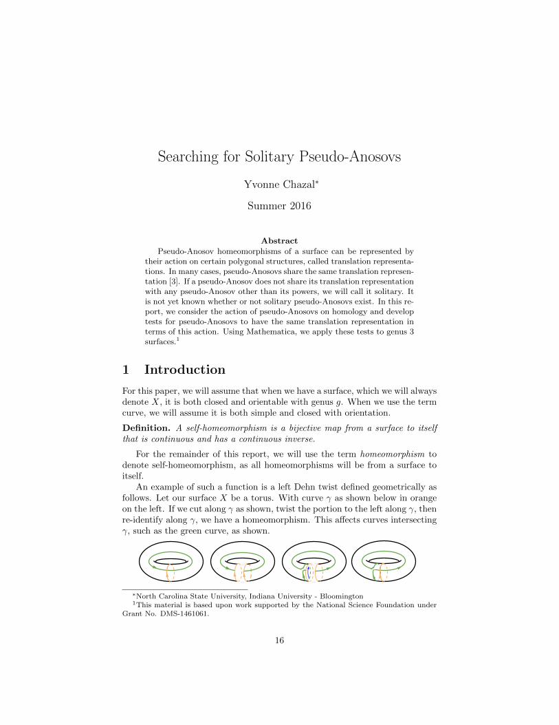
An example of such a function is a left Dehn twist defined geometrically asfollows. Let our surface X be a torus. With curve γ as shown below in orangeon the left. If we cut along γ as shown, twist the portion to the left along γ, thenre-identify along γ, we have a homeomorphism. This affects curves intersectingγ, such as the green curve, as shown.
∗North Carolina State University, Indiana University - Bloomington1This material is based upon work supported by the National Science Foundation under
Grant No. DMS-1461061.
16

The Nielson-Thurston Classification [3] gives a classification for the homeo-morphisms of a surface. A homeomorphism φ is called periodic if there existssome integer k > 0 such that φk = id. φ is called reducible if some power of φmaps a finite union of disjoint simple, closed curves on X back to themselves.
Nielson-Thurston Classification. If φ : X → X is a homeomorphism, oneof the following holds:
1. φ is periodic
2. φ is reducible
3. φ is pseudo-Anosov
The last type of homeomorphism is of particular interest to us, and is thesubject of this project.
Definition. A homeomorphism φ : X → X is called pseudo-Anosov if and onlyif φk(γ) 6= γ for all γ and k > 1.
A self-homeomorphism of a surface can be understood by its action on curveson the surface. If two curves are “parallel,” then their image under the home-omorphism will also be “parallel.” Therefore, we can identify “parallel” curvesusing a notion of “parallel” that is made precise by the homology equivalencerelation.
2 Homology
Definition. Two curves (not necessarily closed) are homologous if their differ-ence bounds a surface.
In the two examples of homologous curves above, we have α (blue) is ho-mologous to β (red), and ∂D = α− β = α ∪ −β, surfaces D colored orange.
Homology is an equivalence relation, meaning we can define equivalencyclasses of homologous curves which we will call homology classes. The homol-ogy class with representative γ will be denoted [γ]. If we take the set of formallinear combinations of curves Σaiγi : ai ∈ Z and mod out by the equivalencerelation, these homology classes form a free abelian group together under addi-tion which we will call the first homology group of X, denoted H1(X,Z) [5]. Ifwe extend this group to consider real coefficients, H1(X,R), it forms a vectorspace.
17

On this vector space, we will need to utilize a basis. The basis we will utilize,which we will discuss further in the next section, will look as follows.
ai, bigi=1 is just one set of representations of our basis elements [ai], [bi]gi=1.Note that for all [ai], [bi]gi=1, aj ∩ bj is only one point and there are no otherintersections. Our first homology group will be all linear combinations of thesebasis elements.
H1(X,R) =
g∑
i=1
mi[ai] + ni[bi] : mi, ni ∈ R
.
For a homeomorphism φ, we can induce a linear homeomorphism φ∗ onthe first homology group. We have that if two curves a1 and a2 are homol-ogous, denoted a1 ∼ a2, then φ(a1) ∼ φ(a2), thus such a function wouldbe well-defined.2 For [γ] = a1[γ1] + a2[γ2] + · · · + ak[γk], define φ∗([γ]) =a1φ∗([γ1]) + a2φ∗([γ2]) + · · ·+ akφ∗([γk]). Thus φ∗ : H1(X,R)→ H1(X,R) is alinear transformation on vector space H1(X,R). We will use φ∗ and its matrixrepresentation, which we will denote Aφ, interchangeably.
Definition. Define i : H1(X,R) × H1(X,R) → R. The intersection form oftwo differentiable curves α and β, denoted i(α, β), is the signed count of timesα and β intersect, where the sign of an intersection is positive if the order ofthe vectors aligns with the orientation of the surface and is negative otherwise.3
Note that i(α, β) = −i(β, α) and that if i(α, γ) = 0 for all γ ∈ X, then αdoes not intersect any curves on the surface, so it must be 0. Also note that forour basis, we have i(ai, bi) = 1 and all other combinations are 0.
Definition. A bilinear form (·, ·) on vector space V is symplectic if and only ifthe following hold:
• If (v, w) = 0 for all w ∈ V , then v = 0.
• (v, w) = −(w, v) for all v, w ∈ V .
Definition. In general, a collection of curves ai, bigi=1 representing basis[ai], [bi]gi=1 will be called a geometric set of representatives if i(aj , bj) = 1
2If α ∼ β, then for a homeomorphism φ, we have φ(α ∪ −β) = φ(∂D), and that φ(α) ∪−φ(β) = ∂φ(D) = ∂D, so φ(α) ∼ φ(β).
3If α and β do not intersect transversely, then we can find homologous curves that do, andthe intersection number does not depend on the homology representative.
18
and there are no other intersections. If [ai], [bi] has a geometric set of repre-sentatives, we will call it a geometric symplectic basis.
Thus, the intersection form is symplectic, and the homology basis that wehave chosen is a geometric symplectic basis.
Definition. A linear transformation L is called symplectic with respect to (·, ·),if and only if (Lx,Ly) = (x, y) for all x, y ∈ V .
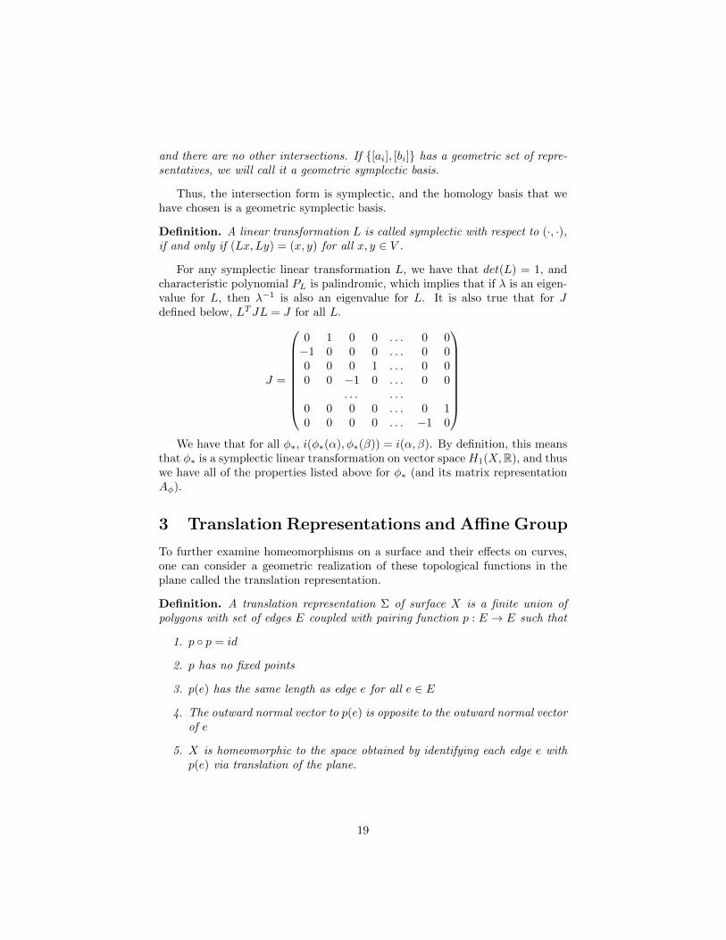
For any symplectic linear transformation L, we have that det(L) = 1, andcharacteristic polynomial PL is palindromic, which implies that if λ is an eigen-value for L, then λ−1 is also an eigenvalue for L. It is also true that for Jdefined below, LTJL = J for all L.
J =
0 1 0 0 . . . 0 0−1 0 0 0 . . . 0 00 0 0 1 . . . 0 00 0 −1 0 . . . 0 0
. . . . . .0 0 0 0 . . . 0 10 0 0 0 . . . −1 0
We have that for all φ∗, i(φ∗(α), φ∗(β)) = i(α, β). By definition, this meansthat φ∗ is a symplectic linear transformation on vector space H1(X,R), and thuswe have all of the properties listed above for φ∗ (and its matrix representationAφ).
3 Translation Representations and Affine Group
To further examine homeomorphisms on a surface and their effects on curves,one can consider a geometric realization of these topological functions in theplane called the translation representation.
Definition. A translation representation Σ of surface X is a finite union ofpolygons with set of edges E coupled with pairing function p : E → E such that
1. p p = id
2. p has no fixed points
3. p(e) has the same length as edge e for all e ∈ E
4. The outward normal vector to p(e) is opposite to the outward normal vectorof e
5. X is homeomorphic to the space obtained by identifying each edge e withp(e) via translation of the plane.
19
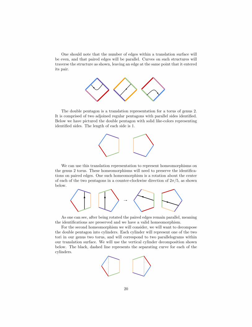
One should note that the number of edges within a translation surface willbe even, and that paired edges will be parallel. Curves on such structures willtraverse the structure as shown, leaving an edge at the same point that it enteredits pair.
The double pentagon is a translation representation for a torus of genus 2.It is comprised of two adjoined regular pentagons with parallel sides identified.Below we have pictured the double pentagon with solid like-colors representingidentified sides. The length of each side is 1.
We can use this translation representation to represent homeomorphisms onthe genus 2 torus. These homeomorphisms will need to preserve the identifica-tions on paired edges. One such homeomorphism is a rotation about the centerof each of the two pentagons in a counter-clockwise direction of 2π/5, as shownbelow.
As one can see, after being rotated the paired edges remain parallel, meaningthe identifications are preserved and we have a valid homeomorphism.
For the second homeomorphism we will consider, we will want to decomposethe double pentagon into cylinders. Each cylinder will represent one of the twotori in our genus two torus, and will correspond to two parallelograms withinour translation surface. We will use the vertical cylinder decomposition shownbelow. The black, dashed line represents the separating curve for each of thecylinders.
20

We are now able to look at homeomorphisms along each of these two cylin-ders, representing homeomorphisms acting on each of the two tori in the surface.We will call the cylinder bounded by the purple, green, and tan edges and theseparating curve the “inner” cylinder. The “outer” cylinder is bounded by thered and blue edges and the separating curve.
Definition. A homeomorphism is called affine with respect to a translationrepresentation Σ if and only if φ is differentiable and the Jacobian dφ does notdepend on the point at which it is taken.
Proposition 1. For each affine homeomorphism φ on surface X, we have dφ ∈SL2(R).
Proof. By the Change of Variables formula, we have
∫
X
dA =
∫
φ(X)
det(dφ)dA
Because φ is a bijective self-homeomorphism, φ(X) = X, so
∫
φ(X)
det(dφ)dA =
∫
X
det(dφ)dA = det(dφ)
∫
X
dA
Thus, by dividing out by the integral, we have that det(dφ) = 1.
If φ is an affine homeomorphism and γ : [0, 1] → R2 is a path, then (φ γ)is also a path. From the Chain Rule, we have
(φ γ)′ = d(φ γ) = (dφ) γ′
It follows by the Fundamental Theorem of Calculus that
(φ γ)(t)− (φ γ)(0) =∫ t0(φ γ)′(s)ds
=∫ t0dφ γ′(s)ds
= dφ∫ t0γ′(s)ds
= dφ(γ(t)− γ(0))
Thus we have
φ γ(t) = dφ(γ(t))− dφ(γ(0)) + φ γ(0)
We can combine the vectors that do not depend on t and call it c ∈ R2, makingour equation
φ(γ) = dφ · γ + c
Note that if γ is a line segment, then φ(γ) is also a line segment.
21

In order to decompose our representation into cylinders, we can cut along theseparating curve, and identify the red and purple edges via translation. Thenwe can make two more cuts (along the pictured blue dashed lines), and identifythe remaining blue and green edges.
Using basic geometry, we can find the heights and widths of each cylinderas we have thus far preserved the geometric structure of our translation repre-sentation. The moduli of the two cylinders (height/width) are
2 sin( 3π10 )
cos( 3π10 )
= 2.7528 . . .2(1 + sin( π10 ))
cos( π10 )= 2.7528 . . .
Suppose we have the orange, straight line shown below on each copy of thetranslation representation, with points along the black dotted line (our sepa-rating curve) identified. For a homeomorphism, the points will need to remainidentified. The two yellow curves below represent the image of the orange curveunder two valid homeomorphisms.
On the left, the two points remain identified, but the yellow curve is notdifferentiable, and thus it is not affine. On the right, the yellow curve is astraight line, with slope equivalent to the modulus of each of the cylinders. Itis because the moduli of these cylinders are rational multiples of each other,namely equivalent, that we are able to produce such a straight line.
The affine homeomorphism shown to the right above is the second home-omorphism we will consider–the left Dehn multitwist–on each of the two torirepresented by the two cylinders above. This will be a left Dehn twist aboutboth b1 and b2.
22
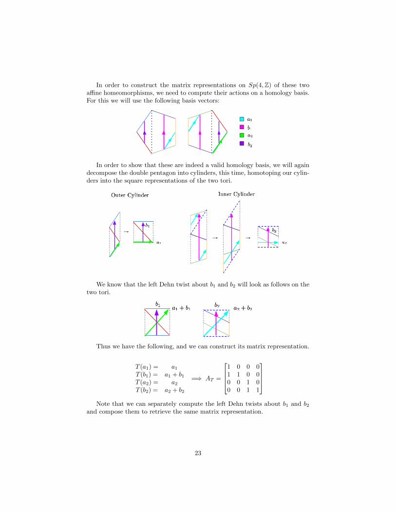
In order to construct the matrix representations on Sp(4,Z) of these twoaffine homeomorphisms, we need to compute their actions on a homology basis.For this we will use the following basis vectors:
In order to show that these are indeed a valid homology basis, we will againdecompose the double pentagon into cylinders, this time, homotoping our cylin-ders into the square representations of the two tori.
We know that the left Dehn twist about b1 and b2 will look as follows on thetwo tori.
Thus we have the following, and we can construct its matrix representation.
T (a1) = a1T (b1) = a1 + b1T (a2) = a2T (b2) = a2 + b2
=⇒ AT =
1 0 0 01 1 0 00 0 1 00 0 1 1
Note that we can separately compute the left Dehn twists about b1 and b2and compose them to retrieve the same matrix representation.
23

ATb1ATb2
=
1 0 0 01 1 0 00 0 1 00 0 0 1
1 0 0 00 1 0 00 0 1 00 0 1 1
=
1 0 0 01 1 0 00 0 1 00 0 1 1
= ATb
As for the rotation, when applied to the homology basis, we get the following.
In order to determine the homology class of these curves, we must again splitthe structure into tori, but we must be careful with the curves that traverse theseparating curve. For these, we must divide the curve into two curves that cancelalong the separating curve. The sum of these two curves will be homologicallyequivalent to our original curve. We also want the curves to turn in the samedirection each time they run into the separating curve. We have chosen for thecurves to turn in the counter-clockwise direction, consistent with the standardorientation. This is shown below.
We can homotope each cylinder into their square representations, homotop-ing R(a1), R(b1), R(a2), and R(b2) along with them. Below we have each of thefour curves split into the two tori and homotoped to the square representations.They are each on their own square representation to reduce clutter. From here,it is fairly easy to see the decomposition of these curves into the basis elements.
24
Thus, we have
R(a1) = −a1 + b1R(b1) = −2a1 + b1 − a2 + b2R(a2) = −a2 + b2R(b2) = −a1 + b1 − a2
=⇒ AR =
−1 −2 0 −11 1 0 10 −1 −1 −10 1 1 0
The Dehn multitwist is classified as reducible, as each time the function isapplied, b1 and b2 remain fixed. The rotation is of finite order, as every powerof 5 will be the identity when the pentagons are rotated a full 2π. Thus neitherof these homeomorphisms constitute pseudo-Anosovs. However, we can findpseudo-Anosovs in combinations of T and R.
The affine self-homeomorphisms of a translation representation Σ constitutea group together with composition called the affine group of Σ, denoted Aff(Σ).
Definition. Two pseudo-Anosov homeomorphisms φ : X → X and ψ : X → Xare called friends if there exists Σ such that φ, ψ ∈ Aff(Σ).
Note that φk is friends with φ for all integers k 6= 0.
Definition. φ is called solitary if and only if Aff(Σ) = 〈φ〉.By this definition, φ and its powers are the only affine homeomorphism
associated with the translation representation Σ. Such homeomorphisms areexactly what we are searching for.
4 Function h
Now that we have a geometric structure of homeomorphisms on a given surface,it is natural to construct a geometric measure on this structure. We will definea linear functional h : H1(X,R) → R2 with respect to translation surface Σ asfollows.
h(γ) =
[hx(γ)hy(γ)
]=
[∫γdx∫
γdy
]
This function measures the amount γ travels in the direction of ex and eyrespectively and provides us with a geometric measure for γ.
h is a linear transformation , as both hx and hy are integral functions, andare thus linear. To construct the matrix representation of this linear transfor-mation, we only need to see what this function does to the basis elements onthe translation structure Σ of surface X. Thus we have the following:
Bh =
h(a1) h(b1) . . . h(a2g) h(b2g)
=
[hx(a1) hx(b1) . . . hx(a2g) hy(b2g)hy(a1) hy(b1) . . . hy(a2g) hy(b2g)
]
25
These values are easily computed from the geometry of the translation struc-ture of a surface, by calculating the length of each ai and bi in directions x andy.
Proposition 2. For translation representation Σ of surface X, h : H1(X,R)→R2 is surjective.
Proof. Proceed by contradiction. Assume hx(γ) = 0 for all γ ∈ H1(X,Z). Fixa point p0 in Σ, and let p be another point on Σ. Note that p could be locatedon a different polygon from p0.
Let α and β be paths in Σ, joining points p0 and p. These paths may be acollection of paths inside multiple polygons such that when the edges of thesepolygons are identified, the paths form one continuous path from p0 to p. α∪−βis a closed curve, and thus represents an element of H1(X,Z). By our initialassumption, we have hx(α ∪ −β) = 0, and thus:
∫
α
dx−∫
β
dx =
∫
α∪−βdx = hx(α ∪ −β) = 0
so∫α∪−β dx is independent of path.
Let us define f : X → R by p 7→∫αdx. It is clear that f is differentiable.
The union of finitely many polygons is a closed and bounded set. Thus,by the Heine-Borel theorem, Σ is compact, so because f is continuous, f mustreach a maximum value at some pmax ∈ Σ, i.e. f(pmax) is the largest value forf .
Consider the following three cases:
1. Suppose (by contradiction) that pmax belongs to the interior of a polygonin Σ. Then there exists ε > 0 such that for t ∈ [0, ε], point pmax +(t, 0) belongs to the polygon containing pmax. If we integrate dx over theconcatenation of the path from p0 to p with the path t 7→ pmax + (t, 0),we have
f(pmax + (ε, 0)) = f(pmax) + ε > f(pmax)
This is a contradiction as f(pmax) is the maximum value for f .
2. Suppose (by contradiction) that pmax belongs to the interior of an edge eof a polygon in Σ. Then the maximum value of f is achieved at everypoint along e. Thus e is parallel to the y-axis and the outward normalvector of e is (1, 0). Let T be the translation identifying e with p(e). Thenthe outward normal vector of p(e) is (−1, 0). pmax is on the interior of e,so T (pmax) is on the interior of p(e)=T (e). Then there exists ε > 0 suchthat for t ∈ [0, ε], point T (pmax+(t, 0)) belongs to the polygon containingedge p(e). If we integrate dx over the concatenation of the path from p0to p with the path t 7→ T (pmax + (t, 0)), we have
f(T (pmax) + (ε, 0)) = f(pmax) + ε > f(pmax)
This is a contradiction as f(pmax) is the maximum value for f .
26
3. Suppose (by contradiction) that pmax is a vertex of a polygon in Σ. Thenpmax may be identified with multiple vertices. Let v1, v2, . . . , vk be ver-tices identified with pmax, with polygons P1, P2, . . . , Pk containing thosevertices and translations T1, T2, . . . , Tk identifying those polygons. Let Pbe the polygon containing point pmax. The union of P and all of theimages of Ti(Pi) contains an open disk centered at pmax. Thus Ti(pmax)is a point on polygon Pi. Then there exists ε > 0 such that for t ∈ [0, ε],point Ti(pmax + (t, 0)) belongs to polygon Pi. If we integrate dx over theconcatenation of the path from p0 to p with the path t 7→ Ti(pmax+(t, 0)),we have
f(Ti(pmax) + (ε, 0)) = f(pmax) + ε > f(pmax)
This is a contradiction as f(pmax) is the maximum value for f .
Therefore, our initial assumption that hx(γ) = 0 for all γ ∈ H1(X,Z) mustbe false. Then there exists γx ∈ H1(X,Z) such that hx(γx) 6= 0.
Let a = hx(γx) and b = hx(γx). Then we have
∫
γ
b · dx− a · dy = b
∫
γx
dx− a∫
γx
dx = b · hx(γx)− a · hx(γx) = ba− ab = 0
Let ω = b·dx−a·dy. Apply the argument above to ω, making the assumptionthat
∫αω = 0 for all paths α. Creating a similar function f gives a gradient
vector field in the direction (b,−a) at the maxima of f . By the argument above,there exists γω ∈ H1(X,Z) such that
∫γωω 6= 0. Because
∫γxω = 0, h(γω) is
independent of h(γx) = (a, b). Thus, the dimension of Im(h) is at least 2, sobecause R2 is two dimensional, h is surjective.
In addition to our original definition of hx and hy, we have its relation tothe intersection number.
hx(γ) =
∫
γ
dx = i(γ, h∗x) (1)
So what is this h∗x? Let’s look at γ = ai and γ = bi. Recall, h∗x ∈ H1(X,R),so h∗x = m1a1 + n1b1 + · · ·+mgag + ngbg.
γ = ai =⇒ hx(ai) = i(ai, h∗x) = i(ai,m1a1 + n1b1 + · · ·+mgag + ngbg)
= m1i(ai, a1) + n1i(ai, b1) + · · ·+mgi(ai, ag) + ngi(ai, bg) = nii(ai, bi) = ni
=⇒ ni = hx(ai)
γ = bi =⇒ hx(bi) = i(bi, h∗x) = i(bi,m1a1 + n1b1 + · · ·+mgag + ngbg)
= m1i(bi, a1) + n1i(bi, b1) + · · ·+mgi(bi, ag) + ngi(bi, bg) = mii(bi, ai) = −mi
=⇒ mi = −hx(bi)
and similarly for h∗y. Thus, we have
27

h∗x = −hx(b1)a1 + hx(a1)b1 + · · · − hx(bg)ag + hx(ag)bg
=
g∑
i=1
−hx(bi)ai + hx(ai)bi
h∗y =
g∑
i=1
−hy(bi)ai + hy(ai)bi.
Combining our definition of h and hx in terms of h∗x (as well as hy), we have
h(γ) =
[i(γ, h∗x)i(γ, h∗y)
].
Proposition 3. h∗x, h∗y span ker(h)⊥.
Proof. For all curves γ in ker(h), h(γ) = (0, 0). By definition of h, this meanshx(γ) = 0 and hy(γ) = 0. Thus i(γ, h∗x) = 0 and i(γ, h∗y) = 0 for all γ ∈ ker(h).
By definition of ⊥, this means that h∗x, h∗y ∈ ker(h)⊥.
Suppose (by contradiction) that h∗x and h∗y are not linearly independent.Then there exists some constant c such that h∗y = c ·h∗x. If this is the case, thenwe have
h(γ) =
[i(γ, h∗x)i(γ, h∗y)
]=
[i(γ, h∗x)c · i(γ, h∗x)
]=
[1 · i(γ, h∗x)c · i(γ, h∗x)
]= i(γ, h∗x)
[1c
]
Therefore, for all γ, h(γ) is a multiple of
[1c
]. Thus, the image of h lies in
the line spanned by
[1c
]. Thus Im(h) has dimension 1. But this contradiction
because from Proposition 2, we have that Im(h) has dimension 2. Thus, h∗x andh∗y are linearly independent.
Because h is surjective, ker(h) has dimension 2g − 2, by the Rank-NullityTheorem. A general fact in symplectic linear algebra gives us that dim(ker(h))+dim(ker(h)⊥) = 2g. Therefore, ker(h)⊥ has dimension 2. Because h∗x and h∗yare in ker(h)⊥ and are linearly independent, they span ker(h)⊥.
Theorem 1. Let φ : Σ → Σ be an affine homeomorphism, inducing a linearfunction φ∗ : H1(X,R) → H1(X,R), and let α : [0, 1] → Σ be a simple, closedcurve with homology class [α] ∈ H1(X,R). Then h(φ∗ α) = dφ · h(α).
Proof. [0, 1] ⊂ R is spanned by a standard basis vector et, which we can thinkof as 1. Σ ⊂ R2 is spanned by standard basis vectors ex, ey.
hx φ∗([α]) = hx([φ α])
28
As stated in Fulton’s Algebraic Topology, for all α ∼ β,∫αdx =
∫βdx [1], so
when considering a homology class, we need only look at a single representative.Here, we will examine φ ∈ [φ] and α ∈ [α]. By definition, we have
hx(φ α) =
∫
φαdx
We can then use the following theorem from Guillemin-Pollack’s DifferentialTopology [2]:
Change of Variables in R2 . If U and V are open subsets of Rk, f : U → Vis an orientation-preserving diffeomorphism, and ω is an integrable k-form onU , then
∫Uω =
∫Vf∗ω.
Here, f∗ is the transpose map of f , and f∗ω is called the pullback of ω byf . In our case, this gives us
∫
φαdx =
∫ 1
0
(φ α)∗dx (2)
Let us consider the integrand here pointwise, where v ∈ Tt0([0, 1]) for t0 ∈[0, 1]. By the definition of pullback of dx by φ α [2],
(φ α)∗(dx)(φα)(t0)(v) = v · (φ α)∗(dx)(φα)(t0)(et) (3)
We will drop v for now and retrieve it later. It follows from the definition oftranspose map [2]
(φ α)∗(dx)(φα)(t0)(et) = (dx)(φα)(t0)
[∂((φ α)x)t0
dt(dt) +
∂((φ α)y)t0dt
(dt)
]
=∂((φ α)x)t0
dt
Retrieving v from (3),
v · (φ α)∗(dx)(φα)(t0)(et) = v · ∂((φ α)x)t0dt
= (dt)t0(v) · ∂((φ α)x)t0dt
=∂((φ α)x)t0
dt(dt)t0(v)
From here, we can distribute x, as it will “trickle down” through the partials,then we can apply the chain rule.
29

=∂(φx αx)t0
dt(dt)t0(v)
=(∂φx)(φα)(t0) · (∂αx)t0
dt(dt)t0(v)
Thus, we have
(φ α)∗(dx)(φα)(t0)(v) =(∂φx)(φα)(t0) · (∂αx)t0
dt(dt)t0(v) ∀v ∈ Tt0([0, 1])
And because we have equality pointwise on the whole interval, we have thatthe functions are equivalent.
(φ α)∗(dx)(φα)(t0) =(∂φx)(φα)(t0) · (∂αx)t0
dt(dt)t0
Returning to (2) with our integral, we now have
∫ 1
0
(φ α)∗dx =
∫ 1
0
(∂φx)(φα)(t0) · (∂αx)t0dt
(dt)t0(v)
However, because φ is an affine homeomorphism, ∂(φx) does not depend ont. Thus, we have
∫ 1
0
(∂φx)(φα)(t0) · (∂αx)t0dt
(dt)t0(v) = ∂φx
∫ 1
0
(∂αx)t0dt
(dt)t0
However, we have that
∫ 1
0
(∂αx)t0dt
(dt)t0 =
∫ 1
0
α∗(dx)
By retrieving ∂φx, applying the Change of Variables Theorem, and usingthe definition of h, respectively
∂φx ·∫ 1
0
α∗(dx) = ∂φx ·∫
α
dx = ∂φx · hx(α)
Thus, we have
hx(φ α) = ∂φx · hx(α)
Using the same procedure with hy,
hy(φ α) = ∂φy · hy(α)
30
then we have the following:
h(φ∗ α) =
[hx(φ∗ α)hy(φ∗ α)
]=
[∂φx · hx(α)∂φy · hy(α)
]= dφ ·
[hx(α)hy(α)
]= dφ · h(α)
To further demonstrate the relationship between h, φ∗, and dφ, consider thefollowing commutative diagram. In this case, we say h intertwines φ∗ and dφ.
H1(X,R) H1(X,R)
R2 R2
φ∗
h h
dφ
Let us now switch to thinking of φ∗ as its matrix representation Aφ. Thuswe have
h(Aφ · v) = dφ · h(v) (4)
Suppose Aφ has eigenvalue λ with corresponding eigenvector v∗. We then havethe following:
dφ · h(v∗) = h(Aφ · v∗) = h(λv∗) = λ · h(v∗) (5)
Of course v∗ could be in the kernel of h, making h(v∗) = 0, and thus makingthe equation trivial. However, if this is not the case, then λ is an eigenvalue forboth Aφ and dφ, and h(v∗) is an eigenvector of dφ. And vectors that satisfythese conditions are of particular interest to us.
Theorem 2 (Thurston [3]). A homeomorphism φ ∈ Aff(Σ) is pseudo-Anosovif and only if |tr(dφ)| > 2.
Proposition 4. If φ ∈ Aff(Σ) is pseudo-Anosov, then Aφ has two distincteigenpairs (λ+, v+) and (λ−, v−) such that the following hold true:
1. v+, v− ∈ ker(h)⊥
2. h(v+) and h(v−) are eigenvectors of dφ
3. |λ+ + λ−| > 2
4. λ+ · λ− = 1.
Proof. We will first consider the pullback of dx and dy by φ. Note that there isa difference between φ∗ and φ∗.
φ∗(dx) = dφx =∂φxdx
dx+∂φxdy
dy
φ∗(dy) = dφy =∂φydx
dx+∂φydy
dy
31
Let F denote the vectors space of 1-forms of the form a·dx+b·dy where a, b ∈ R.Then φ∗ acts on F in the following way.
φ∗(a · dx+ b · dy) = a∂φx
∂x dx+ b∂φx
∂y dy + a∂φy
∂x dx+ b∂φy
∂y dy
=
[a∂φx
∂x dx+ b∂φx
∂y dy
a∂φy
∂x dx+ b∂φy
∂y dy
]
=
[∂φx
∂x∂φx
∂y∂φy
∂x∂φy
∂y
] [ab
]= (dφ)T
[ab
]
If the reader will recall, dφ is the Jacobian of φ. Because φ is an affine, pseudo-Anosov homeomorphism, we have that dφ exists and has |tr(dφ)| > 2. Becausedet(dφ) = 1, dφ is conjugate to a diagonal matrix with its two eigenvalues alongthe diagonal. Thus the determinant, 1, is the product of the two eigenvalues,so the eigenvalues are inverses, say λ and λ−1. Trace is also preserved byconjugation, so |λ+ λ−1| = |tr(dφ)| > 2.
Because of this, dφT will have eigenvectors, say ω+ and ω− with the sucheigenvalues. Eigenpairs for dφT are also eigenpairs for φ∗, so (λ, ω+) and(λ−1ω−) are eigenpairs for φ∗.
From here onward, we will mainly discuss ω+, but the same arguments can becarried out on ω−. Let ω+ = a+dx+ b+dy. Define a function hω+
: H1(X,R)→H1(X,R) such that
hω+(γ) = a+
∫
γ
dx+ b+
∫
γ
dy = a+hx(γ) + b+hy(γ).
Thus, we have that the following. The matrix C is defined below in-context.
[hω+
hω−
]=
[a+ b+a− b−
] [hxhy
]= C
[hxhy
]
Let h∗ω+∈ H1(X,R) be defined as follows for all curves γ ∈ H1(X,R).
hω+(γ) = i(γ, h∗ω+
) =
∫
γ
ω+
Note that h∗ω+∈ ker(h)⊥ because h∗ω+
∈ spanh∗x, h∗y.It follows that
λi(γ, h∗ω+) = λ
∫
γ
ω+ =
∫
γ
φ∗(ω+)
By the definition of pullback [2],
∫
γ
φ∗(ω+) =
∫
φ∗(γ)ω+
32
By the definition of hω+ , we have
∫
φ∗(γ)ω+ = hω+(φ∗(γ)) = i(φ∗(γ), h∗ω+
)
Because i(·, ·) and φ∗ are symplectic, we have that
i(φ∗(γ), h∗ω+) = i(γ, φ−1∗ (h∗ω+
))
and therefore, λi(γ, h∗ω+) = i(γ, φ−1∗ (h∗γ+)). By basic algebra and the non-
degeneracy of i(·, ·), we have the following for all γ ∈ H1(X,R).
λi(γ, h∗ω+) = i(γ, λh∗ω+
) = i(γ, φ−1∗ (h∗γ+))
=⇒ i(γ, λh∗ω+)− i(γ, φ−1∗ (h∗γ+)) = 0
=⇒ i(γ, λh∗ω+− φ−1∗ (h∗γ+)) = 0
=⇒ λh∗ω+− φ−1∗ (h∗γ+) = 0
=⇒ λh∗ω+= φ−1∗ (h∗γ+)
Thus, we have φ∗(h∗ω+) = λ−1h∗ω+
. By a similar argument, we have φ∗(h∗ω−) =
λh∗ω− . Thus, φ∗ has eigenpairs (λ−1, h∗ω+) and (λ, h∗ω−).
Let v+ = h∗ω+, λ+ = λ−1, v− = h∗ω− , and λ− = λ.
Definition. The eigenvectors and eigenvalues as found in the theorem aboveare called affine.
Definition. Eigenvalues λ1 and λ2 are called hyperbolic if λ1 · λ2 = 1 and|λ1 + λ2| > 2.
Proposition 5. If pseudo-Anosovs φ and ψ are friends, then the affine eigen-vectors of φ and ψ span the same plane.
Proof. If φ and ψ are friends, then they both belong to Aff(Σ) for some trans-lation representation Σ with associated h. Because φ, ψ ∈ Aff(Σ), we havethat their affine eigenvectors are in ker(h)⊥. These eigenvectors are linearlyindependent, and thus span the same plane.
Thus, if the affine eigenvectors of Aφ do not span the same symplectic planeas the affine eigenvectors of any other pseudo-Anosov homeomorphism, thenφ may be solitary. However, this is almost impossible to check as there areinfinitely many homeomorphisms on any given surface.
Let (λ, v+) and (λ−1, v−) be affine eigenpairs for Aφ. By definition of eigen-value, we have Aφv+ = λv+. However, by dividing by both λ and Aφ, we getλ−1v+ = A−1φ v+. Now let us consider A−1φ +Aφ.
(A−1φ +Aφ)v+ = A−1φ v+ +Aφv+ = λ−1v+ + λv+ = (λ−1 + λ)v+
33

Similarly, for v−, we have
(A−1φ +Aφ)v− = A−1φ v− +Aφv− = λv− + λ−1v− = (λ+ λ−1)v−
Thus, we have that (λ−1 + λ) is an eigenvalue of A−1φ +Aφ with eigenspace
〈v+, v−〉. Thus we have that if φ and ψ are friends, and λ, λ−1 and µ, µ−1are affine eigenvalues of Aφ and Aψ respectively, then eigenvalue (λ−1 + λ) of(A−1φ +Aφ) and (µ−1 + µ) of (A−1ψ +Aψ) share common eigenspaces.
Thus, if the sum of the affine eigenvalues of Aφ constitute an eigenspace of(A−1φ + Aφ) that is not shared by that of any other homeomorphism, then Aφdoes not have any friends, and thus may be solitary. However, as before, thisis almost impossible to check. But we are able to use this fact to check forhomeomorphisms that are potentially solitary, by checking them against largenumbers of pseudo-Anosovs.
5 Computing
We used the principles outlined above to explore sets of homeomorphisms thatwe could generate. For all computation, we used Mathematica.
The Burkhardt Generators below span Sp(2g,Z) [4].
Transvection (T ): Factor Rotation (R):
1 0 0 0 . . . 0 01 1 0 0 . . . 0 00 0 1 0 . . . 0 00 0 0 1 . . . 0 0
. . . . . .0 0 0 0 . . . 1 00 0 0 0 . . . 0 1
0 −1 0 0 . . . 0 01 0 0 0 . . . 0 00 0 1 0 . . . 0 00 0 0 1 . . . 0 0
. . . . . .0 0 0 0 . . . 1 00 0 0 0 . . . 0 1
Factor Mix (M): Factor Swap (S1) (1↔ 2):
1 0 0 0 . . . 0 00 1 −1 0 . . . 0 00 0 1 0 . . . 0 0−1 0 0 1 . . . 0 0
. . . . . .0 0 0 0 . . . 1 00 0 0 0 . . . 0 1
0 0 1 0 . . . 0 00 0 0 1 . . . 0 01 0 0 0 . . . 0 00 1 0 0 . . . 0 0
. . . . . .0 0 0 0 . . . 1 00 0 0 0 . . . 0 1
When considering a surface with genus g, there are g− 1 factor swap gener-ators swapping adjacent factors ai, bi ↔ ai + 1, bi + 1 for all 1 ≤ i ≤ g.
In order to generate many symplectic matrices of genus 2 and 3, we tookcombinations of these generators and their inverses in tuples of a certain wordlength. We only considered genus 2 and genus 3.
34

Farb-Margalit assert that we can further dissect these generators into Dehntwists as follows, where Tγ denotes a left Dehn twist about curve γ [4].
Transvection Tb1Factor Rotation Tb1 · Ta1 · Tb1
Factor Mix T−1b1· T−1b2
· Tb2−b1Factor Swap (i↔ i+ 1) (Tai+1 · Tbi+1 · Tai+1−bi · Tai · Tbi)3
After generating the matrices and eliminating duplicates that arose, wechecked for pseudo-Anosovs by checking for both hyperbolic eigenvalues andsatisfaction of the Casson-Bleiler Criteria below, adopted from Farb-Margalit’sPrimer on Mapping Class Groups [4].
Casson-Bleiler Criteria for Pseudo-Anosovs. Suppose φ is a homeomor-phism with symplectic matrix representation Aφ. Let PA(x) be the characteris-tic polynomial for Aφ. If each of the following conditions hold true, then φ ispseudo-Anosov.
1. PA(x) cannot be written as a product of two polynomials that are the char-acteristic polynomials of symplectic matrices.
2. PA(x) is not a cyclotomic polynomial.
3. PA(x) cannot be expressed as a polynomial in xk for any k > 1.
We began by checking all unique characteristic polynomials of matrices gen-erated by combinations of the generators and their inverses. This gave us thefollowing percentage of characteristic polynomials of the specified word lengthsatisfying the Casson-Bleiler Criteria out of the total unique characteristic poly-nomials of that specific word length.
Word Length 3 4 5 6g = 2 16.667% 25.000% 26.000% 58.475%g = 3 0% 0% 17.549% 29.310%
This same set of characteristic polynomials gave us the following percentageof characteristic polynomials that had hyperbolic eigenvectors out of the totalunique characteristic polynomials of that specific word length.
Word Length 3 4 5 6g = 2 16.667% 45.833% 62.000% 71.186%g = 3 0% 25.926% 50.877% 56.0356%
Note the discrepancy in these values. The set of Casson-Bleiler pseudo-Anosovs and the matrices with hyperbolic eigenvectors are not the same, neitheris one a subset of the other. Their relationship is described by the following Venndiagram.
35
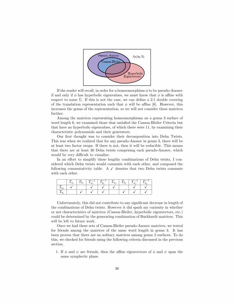
If the reader will recall, in order for a homeomorphism φ to be pseudo-Anosovif and only if φ has hyperbolic eigenvalues, we must know that φ is affine withrespect to some Σ. If this is not the case, we can define a 2:1 double coveringof the translation representation such that φ will be affine [6]. However, thisincreases the genus of the representation, so we will not consider these matricesfurther.
Among the matrices representing homeomorphisms on a genus 3 surface ofword length 6, we examined those that satisfied the Casson-Bleiler Criteria butthat have no hyperbolic eigenvalues, of which there were 11, by examining theircharacteristic polynomials and their generators.
Our first thought was to consider their decomposition into Dehn Twists.This was when we realized that for any pseudo-Anosov in genus 3, there will beat least two factor swaps. If there is not, then it will be reducible. This meansthat there are at least 30 Dehn twists comprising each pseudo-Anosov, whichwould be very difficult to visualize.
In an effort to simplify these lengthy combinations of Dehn twists, I con-sidered which Dehn twists would commute with each other, and composed thefollowing commutativity table. A X denotes that two Dehn twists commutewith each other.
Tai Tbi T−1ai T−1biTaj Tbj T−1aj T−1bj
Tai X X X X X XTbi X X X X X X
Unfortunately, this did not contribute to any significant decrease in length ofthe combinations of Dehn twists. However it did spark my curiosity in whetheror not characteristics of matrices (Casson-Bleiler, hyperbolic eigenvectors, etc.)could be determined by the generating combination of Burkhardt matrices. Thiswill be left to future work.
Once we had these sets of Casson-Bleiler pseudo-Anosov matrices, we testedfor friends among the matrices of the same word length in genus 3. It hasbeen proven that there are no solitary matrices among genus 2 surfaces. To dothis, we checked for friends using the following criteria discussed in the previoussection.
1. If φ and ψ are friends, then the affine eigenvectors of φ and ψ span thesame symplectic plane.
36
2. If φ and ψ are friends, and λ, λ−1 and µ, µ−1 are affine eigenvaluesof Aφ and Aψ respectively, then eigenvalue (λ−1 + λ) of (A−1φ + Aφ) and
(µ−1 + µ) of (A−1ψ +Aψ) share common eigenspaces.
At first, we found that all of the matrices had friends. However, after abit of deliberation, we realized that this was due to the fact that for everymatrix we considered, we were also considering its inverse, which would alwaysconstitute a friendship. Thus, we took out all matrix inverses, both cuttingdown significantly on computation time and giving us more interesting results.
As there were no Casson-Bleiler pseudo-Anosovs for word lengths 3 or 4 ingenus 3, we did not test these word lengths for friends. For word length 5,testing for friends with the first criteria given above, we found that the affineeigenvectors for 54/222 matrices did not share a symplectic plane with the affineeigenvectors of any of the other matrices in word length 5. We found the samenumber of matrices with no friends by the second criteria.
In word length 6, we found that 378 matrices were not friends with any ofthe other 1,928 unique matrices by both the first and second criteria, with 518 ofthese 1,928 having no affine eigenvectors. When the lists of friendless matricesamong word length 5 and word length 6 were concatenated and run through thecode, no additional friendships were found.
It is important to note these matrices may have friends in Casson-Bleilermatrices with longer word lengths, or the may have friends that are pseudo-Anosov, but do not satisfy the Casson-Bleiler Criteria. Thus, we cannot statethat these are solitary pseudo-Anosovs; however, it is possible that there aresolitary pseudo-Anosovs among these matrices.
The next step in our work would be to produce an algorithm for constructingthe translation representations from affine eigenvectors. This would help us toinvestigate why these matrices have no friends among their word length, andperhaps we could construct friends from these translation surfaces in order torule out matrices that are not solitary.
One could also work to make the Mathematica code more efficient. Com-putational time and memory was a limiting factor on what we could do, as thenumber of matrices generated the five generators and their inverses for genus3 is already 1,000,000 matrices for word length 6, increasing tenfold for eachadded word. By eliminating calculations for matrix representations, we couldexpand the number of matrices that we would be able to consider.
References
[1] Fulton, William. Algebraic Topology: A First Course. New York: Springer-Verlag 1995. Print.
[2] Guillemin, Victor, and Alan Pollack. Differential Topology. EnglewoodCliffs: Prentice Hall 1974. Print.
37
[3] Thurston, William P. On the geometry and dynamics of diffeomorphismsof surfaces. Bull. Amer. Math. Soc. (N.S.) 19 (1988), no. 2, 417–431.
[4] Farb, Benson, and Dan Margalit. A Primer on Mapping Class Groups.5.0th ed. Princeton: Princeton UP, 2012. Print.
[5] Hatcher, Allen. Algebraic Topology. Cambridge: Cambridge UP, 2002.Print.
[6] Gutkin, Eugene, and Judge, Chris. Affine mappings of translation surfaces:geometry and arithmetic. Duke Math. J. 103 (2000), no. 2, 191–213.
38
Klein Bottle Constructions
James DixUT Austin
Advisor: Jeffrey MeierIndiana University
September 14, 2016
Abstract
In this report we consider knotted Klein bottles in S4 generated froman inversion of a knot. We use this construction to prove the existence ofa knotted Klein bottle which does not decompose as a connected sum ofan unkotted projective plane and a knotted projective plane.
1 Background
The theory of knotted surfaces is analogous to classical knot theory; it studiesthe smooth embeddings of a surface in S4 up to smooth isotopy. A main reasonthis topic can be difficult to analyze is that the surfaces and isotopies of thesurfaces in S4 are much harder to visualize. One way to describe a knottedsurface Σ is to use a banded link diagram.
A banded link diagram is an unlink in R3 with bands attached so thatsurgering along these bands gives another unlink. To construct a surface fromthis, view the banded link in R3 as a 3-dimensional hyperplane cross-section ofa surface in R4. This cross section splits R4 into R4
+ and R4−. Disks can be
attached in R4− to the pre-surgery unlink in the banded diagram and similarly
disks can be attached in R4+ to the post-surgery unlink. The result of this gluing
is a surface in R4. Using Morse theory, one can show every knotted surface canbe specified by a banded link. The critical points of index of the Morse function0 and 2 correspond to the disks attached in R4
− and R4+, while the critical points
of index 1 correspond to the bands in the banded link diagram. Thus attachingthe correct bands is a matter of finding the saddle points of the surface. Theknot group π1(S4\Σ) can be computed from this diagram using a form of theWirtinger presentation.
The following are some interesting conjectures about knotted surfaces whichwere relevant to our project:
This material is based upon work supported by the National Science Foundation underGrant No. DMS-1461061
39

Figure 1: A banded link diagram
Conjecture 1 (Unkotting Conjecture). Any orientable surface with knot groupZ or any non-orientable surface with knot group Z2 is unkotted.
Conjecture 2. Any knotted projective plane can be decomposed into the con-nected sum of an unkotted projective plane and a knotted sphere.
2 Construction
A half-spun Klein bottle can be constructed using a knot K ⊂ B3 and aninversion of K (an orientation-reversing isotopy). A surface Σ′ in B3 × I iscreated applying the inversion as one proceeds along the interval. AssociatingB3 × 0 with B3 × 1 gives a Klein bottle embedded in B3 × S1. B3 × S1
can then be embedded in the a standard way into S4 to create a knotted Kleinbottle.
The banded link diagram created by this mirrors the diagram created bycreating a knotted torus or a knotted sphere via spinning.
The Klein bottle construction can be thought of as removing the top halfof the spun torus and applying the inversion before re-gluing. For example, thebanded link for the unkotted Klein bottle can be thought of this way. (Insertdiagrams)
When the knot inversion is a simple rotation, the banded link diagram canbe used to show that an unkotted projective plane can be removed as a con-nected summand of the spun Klein bottle. The result is a decomposition of thespun Klein bottle into a knotted projective plane and an unkotted projectiveplane. In fact, this knotted projective matches a construction given by Priceand Roseman, up to a change in Euler number arising from a choice of cross-cap.
Price and Roseman prove that two different inversions of the trefoil canproduce different knotted projective planes. These two inversions also producedifferent knotted Klein bottles. Interestingly, the inversions are the same when
40
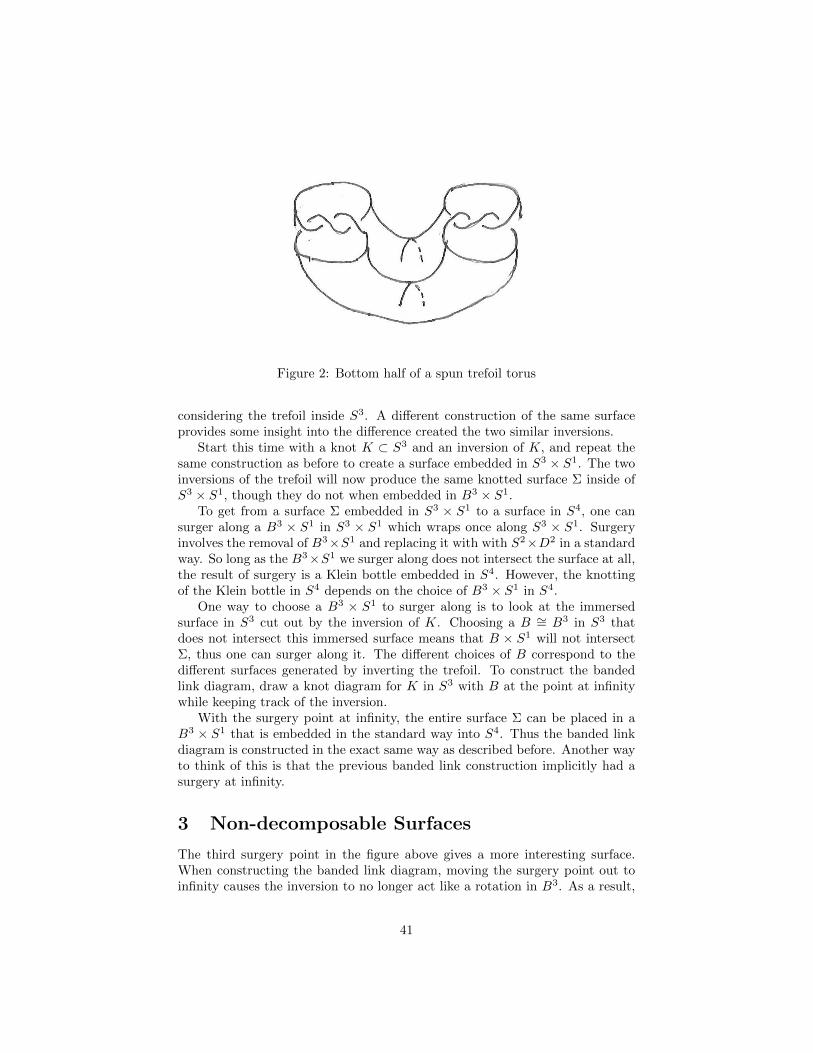
Figure 2: Bottom half of a spun trefoil torus
considering the trefoil inside S3. A different construction of the same surfaceprovides some insight into the difference created the two similar inversions.
Start this time with a knot K ⊂ S3 and an inversion of K, and repeat thesame construction as before to create a surface embedded in S3 × S1. The twoinversions of the trefoil will now produce the same knotted surface Σ inside ofS3 × S1, though they do not when embedded in B3 × S1.
To get from a surface Σ embedded in S3 × S1 to a surface in S4, one cansurger along a B3 × S1 in S3 × S1 which wraps once along S3 × S1. Surgeryinvolves the removal of B3×S1 and replacing it with with S2×D2 in a standardway. So long as the B3×S1 we surger along does not intersect the surface at all,the result of surgery is a Klein bottle embedded in S4. However, the knottingof the Klein bottle in S4 depends on the choice of B3 × S1 in S4.
One way to choose a B3 × S1 to surger along is to look at the immersedsurface in S3 cut out by the inversion of K. Choosing a B ∼= B3 in S3 thatdoes not intersect this immersed surface means that B × S1 will not intersectΣ, thus one can surger along it. The different choices of B correspond to thedifferent surfaces generated by inverting the trefoil. To construct the bandedlink diagram, draw a knot diagram for K in S3 with B at the point at infinitywhile keeping track of the inversion.
With the surgery point at infinity, the entire surface Σ can be placed in aB3 × S1 that is embedded in the standard way into S4. Thus the banded linkdiagram is constructed in the exact same way as described before. Another wayto think of this is that the previous banded link construction implicitly had asurgery at infinity.
3 Non-decomposable Surfaces
The third surgery point in the figure above gives a more interesting surface.When constructing the banded link diagram, moving the surgery point out toinfinity causes the inversion to no longer act like a rotation in B3. As a result,
41
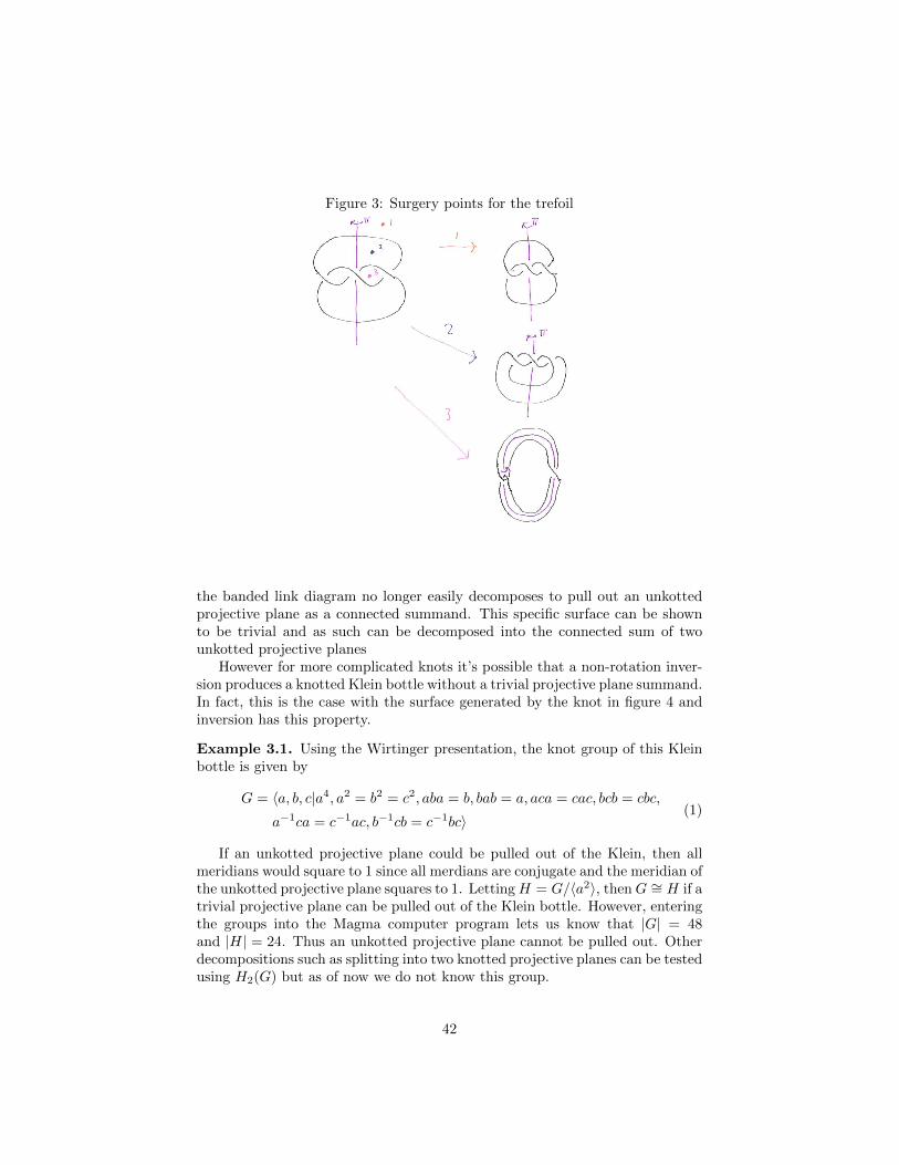
Figure 3: Surgery points for the trefoil
the banded link diagram no longer easily decomposes to pull out an unkottedprojective plane as a connected summand. This specific surface can be shownto be trivial and as such can be decomposed into the connected sum of twounkotted projective planes
However for more complicated knots it’s possible that a non-rotation inver-sion produces a knotted Klein bottle without a trivial projective plane summand.In fact, this is the case with the surface generated by the knot in figure 4 andinversion has this property.
Example 3.1. Using the Wirtinger presentation, the knot group of this Kleinbottle is given by
G = 〈a, b, c|a4, a2 = b2 = c2, aba = b, bab = a, aca = cac, bcb = cbc,
a−1ca = c−1ac, b−1cb = c−1bc〉(1)
If an unkotted projective plane could be pulled out of the Klein, then allmeridians would square to 1 since all merdians are conjugate and the meridian ofthe unkotted projective plane squares to 1. LettingH = G/〈a2〉, thenG ∼= H if atrivial projective plane can be pulled out of the Klein bottle. However, enteringthe groups into the Magma computer program lets us know that |G| = 48and |H| = 24. Thus an unkotted projective plane cannot be pulled out. Otherdecompositions such as splitting into two knotted projective planes can be testedusing H2(G) but as of now we do not know this group.
42
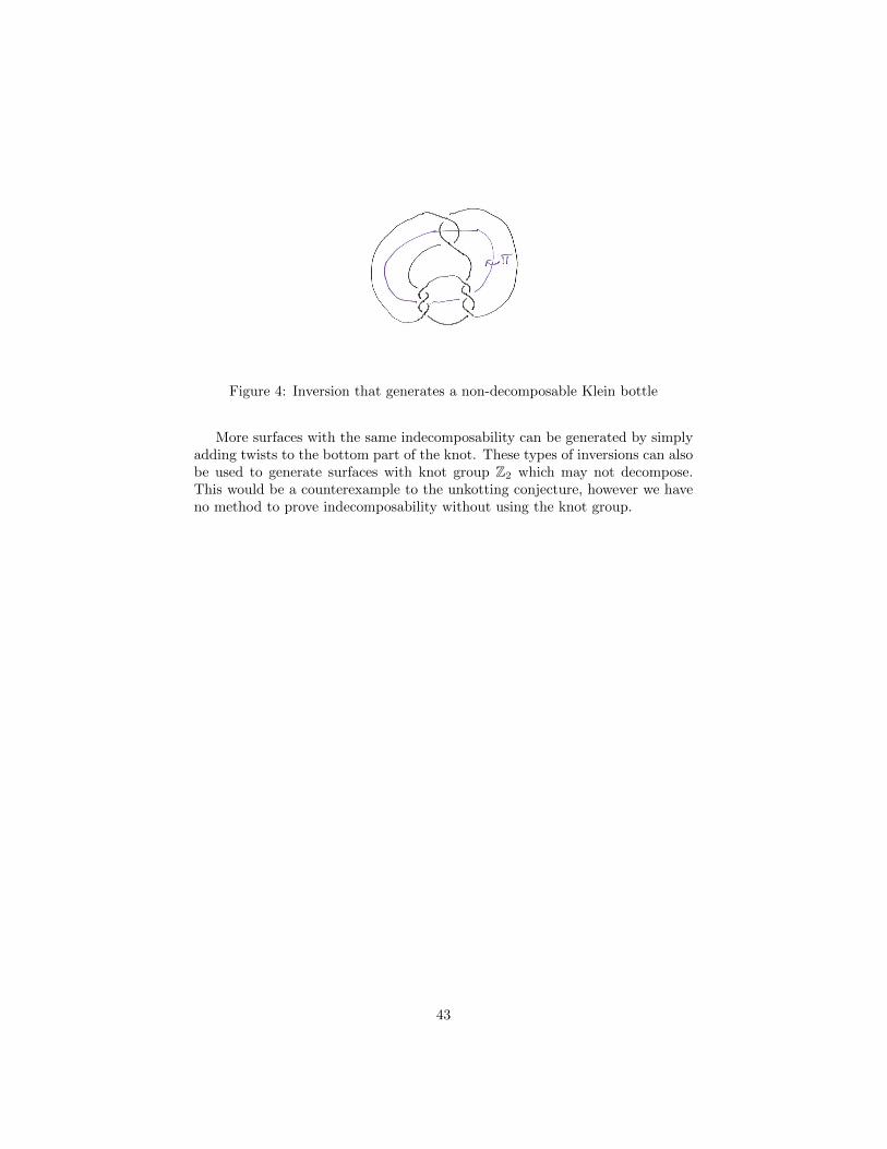
Figure 4: Inversion that generates a non-decomposable Klein bottle
More surfaces with the same indecomposability can be generated by simplyadding twists to the bottom part of the knot. These types of inversions can alsobe used to generate surfaces with knot group Z2 which may not decompose.This would be a counterexample to the unkotting conjecture, however we haveno method to prove indecomposability without using the knot group.
43
On Surfaces that are Intrinsically Surfaces ofRevolution
Daniel FreeseAdvisor: Matthias Weber
September 14, 2016
Abstract
We consider surfaces in Euclidean space parametrized on an an-nular domain such that the first fundamental form and the principalcurvatures are rotationally invariant, and the principal curvature di-rections only depend on the angle of rotation (but not the radius).Such surfaces generalize the Enneper surface. We show that they arenecessarily of constant mean curvature, and that the rotational speedof the principal curvature directions is constant. We classify the min-imal case. The (non-zero) constant mean curvature case has beenclassified by Smyth.
1
1This material is based upon work supported by the National Science Foundation underGrant No. DMS-1461061.
44

1 Introduction
We begin this paper with some background on surface theory and brieflydescribe some of the concepts we cover.
Definition 1.1. Let U ⊂ R2 be an open set. A parametrized surface is animmersion f : U → R3.
We consider the parameters (u, v) ∈ U .Recall that an immersion is a mapping whose Jacobian matrix Jf has
maximal rank, that is, whose columns are linearly independent. When con-sidering a surface parametrization f , this reduces to the vectors ∂f
∂uand ∂f
∂v
being linearly independent at every point.
Definition 1.2. The tangent space of R3 at a point P ∈ R3 is defined tobe the vector space P ×R3 with vector addition and scalar multiplicationdefined as follows:
(P,X) + (P, Y ) = (P,X + Y ), c(P,X) = (P, cX) ∀ X, Y ∈ R3, c ∈ R .
Definition 1.3. Let f : U → R3 be a parametrized surface and p ∈ U . Thevectors ∂f
∂u|p and ∂f
∂v|p form a basis for a 2-dimensional subspace of Tf(p)R3,
which we call the tangent plane Tpf of f at p.
Note that for a point p ∈ U , Tpf is isomorphic to TpU .
Definition 1.4. Given an immersion f : U ⊂ R2 → R3, the isomorphismdf |p : TpU → Tpf defined by
df |p(X) = JpfX
is called the differential or push-forward of f .
The differential relates vectors in the tangent plane of f to the tangentspace of U . We call dfX the directional derivative of f in the X-direction,and also denote it dXf .
Definition 1.5. The symmetric bilinear form Ip : TpU → R defined by
Ip(X, Y ) = 〈df |pX, df |pY 〉 ∀X, Y ∈ TpU
45

is called the first fundamental form of f at p.The first fundamental form is represented as the 2× 2 matrix
I =
(〈∂f∂u, ∂f∂u〉 〈∂f
∂u, ∂f∂v〉
〈∂f∂v, ∂f∂u〉 〈∂f
∂v, ∂f∂v〉
).
The first fundamental form allows us to calculate angles between tangentvectors, as well as their norms. It also allows us to calculate arc length andsurface area. The intrinsic geometry of a surface is the geometry that de-pends only on the first fundamental form. Thus, if two surfaces that havethe same first fundamental form, they have intrinsic geometry. For example,they have the same concept of distance, even if they are different extrinsi-cally. The next notion reveals extrinsic information of the surface.
The unit-normal vector of a surface defined by N =∂f∂u× ∂f∂u
‖ ∂f∂u× ∂f∂u‖ at each point
can be viewed as a mapping into R3, which we call the Gauss map ν.
Definition 1.6. The endomophism Sp : TpU → Tpf defined by
SpX = dν |p (df |p)−1X ∀X ∈ Tpf
is called the shape operator of f at p. It is represented by its standardmatrix.
The shape operator gives us a notion of the curvature of the surface.When studying curves in space we can calculate the curvature of a givencurve, which tells us how much the curve bends. At a point p on a surface,the shape operator tells us the curvature of a curve going in each directionin the tangent plane.
The extremal curvatures are called the principal curvatures, and the di-rections where the curvatures are extremal are called the principal curvaturedirections. These correspond respectively to the eigenvalues and eigenvectorsof the shape operator.
For more detailed background on these concepts, we refer the reader to[4]. As we proceed, we will omit the point-dependence from our notation.
Now we approach the subject of our study.
46
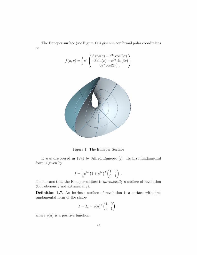
The Enneper surface (see Figure 1) is given in conformal polar coordinatesas
f(u, v) =1
6eu
3 cos(v)− e2u cos(3v)−3 sin(v)− e2u sin(3v)
3eu cos(2v) .
Figure 1: The Enneper Surface
It was discovered in 1871 by Alfred Enneper [2]. Its first fundamentalform is given by
I =1
4e2u(1 + e2u
)2(
1 00 1
).
This means that the Enneper surface is intrinsically a surface of revolution(but obviously not extrinsically).
Definition 1.7. An intrinsic surface of revolution is a surface with firstfundamental form of the shape
I = Iρ = ρ(u)2(
1 00 1
),
where ρ(u) is a positive function.
47
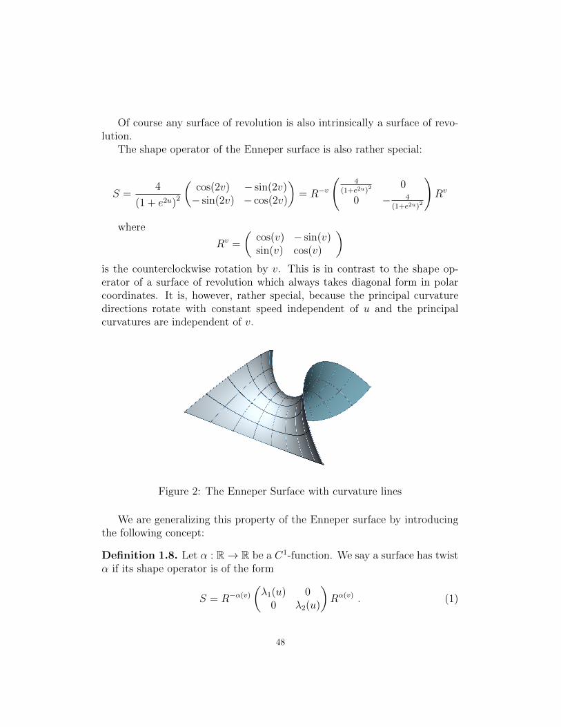
Of course any surface of revolution is also intrinsically a surface of revo-lution.
The shape operator of the Enneper surface is also rather special:
S =4
(1 + e2u)2
(cos(2v) − sin(2v)− sin(2v) − cos(2v)
)= R−v
(4
(1+e2u)20
0 − 4(1+e2u)2
)Rv
where
Rv =
(cos(v) − sin(v)sin(v) cos(v)
)
is the counterclockwise rotation by v. This is in contrast to the shape op-erator of a surface of revolution which always takes diagonal form in polarcoordinates. It is, however, rather special, because the principal curvaturedirections rotate with constant speed independent of u and the principalcurvatures are independent of v.
Figure 2: The Enneper Surface with curvature lines
We are generalizing this property of the Enneper surface by introducingthe following concept:
Definition 1.8. Let α : R→ R be a C1-function. We say a surface has twistα if its shape operator is of the form
S = R−α(v)(λ1(u) 0
0 λ2(u)
)Rα(v) . (1)
48

Note that this precisely means that the principal curvature directions areindependent of u, and the principal curvatures are independent of v.
In summary, the Enneper surface is an example of an intrinsic surfaceof revolution with twist α(v) ≡ v. A standard surface of revolution, on theother hand, has twist α(v) ≡ 0.
Note that while this is a generalization of the minimal Enneper surface,we make no assumption on the principal curvatures, besides their indepen-dence of v.
In this paper, we consider these general intrinsic surfaces of revolutionwith twist α. Our goal is to find conditions on the conformal factor ρ(u) andthe twist function α(v) necessary for these surfaces to exist and to constructand classify these surfaces.
Now we can formulate our main theorem, which is a consequence of theCodazzi equations.
Theorem 1.9. Let Σ be an intrinsic surface of revolution with twist functionα. Assume that α is not identically equal to 0 or any other integral multipleof π/2, on any open interval. Assume furthermore that the surface has noopen set of umbilic points. Then Σ has constant mean curvature, and thetwist function is linear α(v) = av.
Constant mean curvature surfaces that are intrinsic surfaces of revolutionhave been studied by Smyth, see [5]. Thus our result complements Smyth’sresult by replacing his assumption about constant mean curvature with ageometric assumption.
I order to begin a complete classification, we will invoke Bonnet’s theoremto prove:
Theorem 1.10. Let Σ be an intrinsic surface of revolution of constant meancurvature H = λ1 +λ2, first fundamental form Iρ for ρ : (u1, u2)→ R>0, andlinear twist α(v) = av. Then ρ satisfies the differential equation
ρ′(u)2 − ρ(u)ρ′′(u) =1
4H2ρ(u)4 − b2e4au (2)
for a constant b.
49
Vice versa, given H, and α(v) = av, a constant b and ρ satisfying Equa-tion (2), define
λ1,2(u) =1
2H ± b e
2au
ρ(u)2.
Then the first fundamental form Iρ and the shape operator S given by Equa-tion (1) satisfy the Gauss- and Codazzi equations and thus define an intrinsicsurface of revolution with constant twist α(v) = av and constant mean cur-vature H.
In the special case of minimal surfaces, we can achieve a complete classi-fication.
Theorem 1.11. Let Σ be an intrinsic surface of revolution that is also min-imal with constant twist α(v) = av with a > 0. Then Σ belongs to an explicit2-parameter family of minimal surfaces with Weierstrass data given by
G(w) = − 1
AwB and dh =
1
2Bw2a−1 dw ,
with parameters A and B.
In the case that the twist function is α(v) ≡ a = 0, we prove:
Theorem 1.12. Given a conformal factor ρ(u) on an interval u1 < u < u2and a constant c such that c2ρ(u) > |ρ′(u)| for all u1 < u < u2. Then thereis an intrinsic surface of revolution defined on the domain (u1, u2)× R withfirst fundamental form Iρ and twist α(v) ≡ 0. Moreover, this surface can berealized as an actual surface of revolution in R3 of the form
f(u, v) = (g(u) cos(cv), g(u) sin(cv), h(u))
with suitable functions g, h : (u1, u2)× R.
The paper is organized as follows:
• In section 2, we compute the Gauss- and Codazzi equations for intrinsicsurfaces of revolution, reduce them to a single ODE for ρ, and proveTheorems 1.9 and 1.10.
• In section 3, we specialize this equation to the minimal case, integratethe surface equations, find the Weierstrass representation of the sur-faces, prove Theorem 1.11, and give examples.
50
• In section 4, we briefly discuss the constant mean curvature case byconnecting our approach to Smyth’s. While we are not able to find ex-plicit solutions for the Smyth surfaces, we can find numerical solutionsand make images.
• In section 5, we consider the case of twist 0, prove Theorem 1.12, andshow that sectors of the Enneper surface are isometric to sectors (withdifferent angle) of surfaces of revolution.
2 Gauss- and Codazzi equations for intrinsic
surfaces of revolution with twist a > 0
In order to determine when the first fundamental form and shape operatorof an intrinsic surface of revolution with twist function α are induced by anactual surface in R3, we make use of an important theorem of surface theory,Bonnet’s theorem. But first, we’ll introduce some of the machinery behindthis theorem.
We first introduce the covariant derivative. For a surface f and tangentvector fields X, Y on f , the covariant derivative, or Levi-Civita connection,DXY measures how Y varies when it goes along a curve in the X-direction.However, it also acts on general tensor fields on the surface. We present someof its properties, which are useful in the derivations that follow.
Lemma 2.1. Given a surface f , for all tangent vector fields X, Y, Z andendomorphisms F,G of the tangent plane and for every scalar function φalong f , we have
(1) DφXY = φDXY,
(2) DX(φY ) = φDXY + (dXφ)Y,
(3) DXI(Y, Z) = I(DXY, Z) + I(Y,DXZ)
(4) DXY −DYX = [X, Y ] = dXY − dYX,(5) DX(F (Y )) = (DXF )Y + F (DXY )
(6) (DXFG) = (DXF )G+ F (DXG).
where dX is the directional derivative in the X-direction.
51
We refer to these properties by their numbers in what follows.The Gauss- and Codazzi Equations are two essential equations of surfaces
in Euclidean space. These can be written in terms of the covariant derivative,as we will show when we derive their simplified forms.
Bonnet’s theorem states that, given any positive definite first fundamentalform and shape operator satisfying the Gauss- and Codazzi equations, thereexists a unique surface in R3 with these first fundamental form and shapeoperator, up to rigid motion. Thus, we need only derive the Gauss- andCodazzi equations for intrinsic surfaces of revolution with twist α and solvethem to determine the necessary conditions on the first fundamental formand shape operator.
In order to derive the Gauss- and Codazzi equations we first determinethe relevant covariant derivatives. Much of this preparation is standard.
Introduce
U =1
ρ(u)
∂
∂uV =
1
ρ(u)
∂
∂v(3)
as the normalized coordinate vector fields. Their orthonormality with re-spect to Iρ follows from the orthonormality of ∂
∂uand ∂
∂vwith respect to the
standard inner product and the definition of Iρ. Since they form a basis ofR2, our calculations only involve these two vectors. First, we have
Lemma 2.2. The Levi-Civita connection of the first fundamental form Iρ isgiven by
DUU = 0 DUV = 0
DVU =ρ′(u)
ρ(u)2V DV V = − ρ
′(u)
ρ(u)2U .
Proof. By the v-invariance of the first fundamental form, the curves s 7→(s, v) are geodesics, and U is the unit-length tangent vector to these curves.This implies DUU = 0. Next V = Rπ/2U and intrinsic rotations are parallel,so that DUV = 0 as well.
52
Using that D is torsion-free and metric, we compute
DVU = DUV + [V, U ] by (4)
= 0 + dVU − dUV
=∂
ρ(u)∂v
∂
ρ(u)∂u− ∂
ρ(u)∂u
∂
ρ(u)∂v
= − 1
ρ(u)
∂
∂u
∂
ρ(u)∂v
=1
ρ(u)
ρ′(u)
ρ(u)2∂
∂v
=ρ′(u)
ρ(u)2V
and
DV V = I(DV V, U)U + I(DV V, V )V
= dV I(V, U)U − I(V,DVU)U + 0 by (3)
= dV (0)U − I(V,ρ′(u)
ρ(u)2V
)U = − ρ
′(u)
ρ(u)2U,
where I(DV V, V )V = 0 because
I(DV V, V ) = dV I(V, V )V − I(V,DV V )V by (3)
= dV I(V, V )V − I(V,DV V )V
= dV (1)V − I(V,DV V )V = −I(DV V, V )V.
Lemma 2.3. The Gauss equation is equivalent to
λ1(u)λ2(u) =ρ′(u)2 − ρ(u)ρ′′(u)
ρ(u)4.
53

Proof. The Gauss equation gives us:
I(R(U, V )V, U) = det(S) = λ1(u)λ2(u)
where R is the Riemann curvature tensor given by
R(X, Y ) = DXDY −DYDX −D[X,Y ]
for all tangent vector fields X, Y .Let us calculate R(U, V )V .
R(U, V )V = DUDV V −DVDUV −D[U,V ]V
= DU
(− ρ
′(u)
ρ(u)2U
)−DV (0)−D− ρ′(u)
ρ(u)2VV
= − ρ′(u)
ρ(u)2DUU − dU
(ρ′(u)
ρ(u)2
)U +
ρ′(u)
ρ(u)2DV V by (2) & (1)
= 0− 1
ρ(u)
∂
∂u
(ρ′(u)
ρ(u)2
)U +
ρ′(u)
ρ(u)2
(− ρ
′(u)
ρ(u)2U
)
= − 1
ρ(u)
(ρ′′(u)ρ(u)2 − ρ′(u)(2ρ(u)ρ′(u))
ρ(u)4
)U − ρ′(u)2
ρ(u)4U
=−ρ′′(u)ρ(u) + 2ρ′(u)2 − ρ′(u)2
ρ(u)4U
=ρ′(u)2 − ρ(u)ρ′′(u)
ρ(u)4U ,
and the claim follows.
In order to derive the Codazzi equations, we need to compute a few morecovariant derivatives regarding some endomorphisms of the tangent plane.
Lemma 2.4. The covariant derivatives of the twist rotation are given by
DURα(v) = 0 and DVR
α(v) =α′(v)
ρ(u)Rα(v)+π
2 .
Proof. The first equations follows because intrinsic rotations by a constant
54
angle are parallel and α is independent of u. For the second, we have,
(DVRα(v))U = DV (Rα(v)U)−Rα(v)DVU by (5)
= DV (cos(α(v))U + sin(α(v))V )− ρ′(u)
ρ(u)2Rα(v)V
= dV (cos(α(v))U + cos(α(v)DVU + dV (sin(α(v)))V + sin(α(v))DV V
− ρ′(u)
ρ(u)2(− sin(α(v))U + cos(α(v))V ) by (2)
=1
ρ(u)
(∂
∂vcos(α(v)U +
∂
∂vsin(α(v)V
)+ cos(α(v)DVU + sin(α(v))DV V
− (sin(α(v))DV V + cos(α(v))DVU)
=1
ρ(u)(−α′(v) sin(α(v)U + α′(v) cos(α(v))V )
=α′(v)
ρ(u)
(cos(α(v) +
π
2
)U + sin
(α(v) +
π
2
)V)
=α′(v)
ρ(u)Rα(v)+π
2U ,
and likewise DVRα(v)V = α′(v)
ρ(u)Rα(v)+π
2 V .
Lemma 2.5. The covariant derivatives of the eigenvalue endomorphism Λare given by
DUΛ(u) =1
ρ(u)Λ′(u)
(DV Λ(u))U =ρ′(u)
ρ2(u)(λ1(u)− λ2(u))V
(DV Λ(u))V =ρ′(u)
ρ2(u)(λ1(u)− λ2(u))U .
Proof. First note that ΛU = λ1U and ΛV = λ2V . We derive the first
55

equation as follows:
(DUΛ)U = DU(ΛU)− ΛDUU
= DU(λ1U)− Λ0
= (dUλ1)U + λ1DUU by (2)
=1
ρ
∂λ1∂u
U + 0
=1
ρλ1U =
1
ρ(u)Λ′(u)U ,
and likewise (DUΛ)V = 1ρ(u)
Λ′(u)V .For the second, we compute
(DV Λ)U = DV (λ1U)− ΛDVU
= λ1DVU − λ2DVU
=ρ′(u)
ρ2(u)(λ1(u)− λ2(u))V .
The third equation is proven the same way.
Lemma 2.6. The covariant derivatives of the shape operator are given by
(DUS)V =1
ρ(u)R−α(v)Λ′(u)Rα(v)V
(DV S)U = (λ1(u)− λ2(u))ρ′(u)− ρ(u)α′(v)
ρ2(u)R−2α(v)V .
Proof. In the statement, we have indicated the dependence of each functionby their respective variables. To improve legibility, we will drop the variablesin the computations below. Observe, however, that derivatives like α′ and ρ′
are always taken with respect the proper variables.For both equations we differentiate the definition of S according to the
56
product rule, and then use the lemmas above. For the first equation, we have
(DUS)V = DU(R−αΛRα)V
= (DU(R−α)ΛRα + V +R−αDU(Λ)Rα +R−αΛ(DURα))V by (6)
= (0 +R−αDU(Λ)Rα + 0)V
=1
ρ(u)R−α(v)Λ′(u)Rα(v)V .
For the second, we obtain
(DV S)U = DV (R−αΛRα)(U)
=((DVR
−α)ΛRα +R−α(DV Λ)Rα +R−αΛ(DVRα))
(U)
= R−α(−α
′
ρR
π2 ΛRα + (DV Λ)Rα +
α′
ρΛRα+π
2
)(U)
= R−α(−α′
ρR
π2 Λ(cos(α)U + sin(α)V )+
(DV Λ)(cos(α)U + sin(α)V ) +α′
ρΛ(− sin(α)U + cos(α)V ))
= R−α(−α′
ρR
π2 (λ1 cos(α)U + λ2 sin(α)V )+
ρ′
ρ2(λ1 − λ2)(cos(α)V + sin(α)U) +
α′
ρ(−λ1 sin(α)U + λ2 cos(α)V ))
= (λ2 − λ1)(−α′
ρ+ρ′
ρ2)R−α(− sin(α)U − cos(α)V )
= (λ1 − λ2)(−α′
ρ+ρ′
ρ2)R−2αV
Corollary 2.7. The Codazzi equations are equivalent to
(λ′1 + λ′2) sin(α) cos(α) = 0
1
ρ(λ1 − λ2)(ρ′ − ρα′) = −λ′1 sin2(α) + λ′2 cos2(α)
57
Proof. The Codazzi equations state that (DXS)Y = (DY S)X for any pairof tangent vectors X and Y . As we are in dimension 2 and the equation issymmetric, it suffices to verify this for X = U and Y = V . By the previoustheorem, this is equivalent to
ρΛ′RαV = (λ1 − λ2)(ρ′ − ρα′)R−αV
Pairing both sides with I(·, R−αU) and I(·, R−αV ) respectively gives
ρI(Λ′RαV,R−αU) = 0
ρI(Λ′RαV,R−αV ) = (λ1 − λ2)(ρ′ − ρα′)
as rotations preserve I, which gives I(R−αV,R−αU) = I(V, U) = 0 andI(R−αV,R−αV ) = 1.
The first equation simplifies to
0 = I(−Λ′(sin(α)U + cos(α)V ), cos(α)U − sin(α)V )
= I(−λ′1 sin(α)U + λ′2 cos(α)V ), cos(α)U − sin(α)V )
= −(λ′1 + λ′2) sin(α) cos(α),
giving us the first result, and the second to
1
ρ(λ1 − λ2)(ρ′ − ρα′) = I(Λ′RαV,R−αV )
= I(−λ′1 sin(α)U + λ′2 cos(α)V ), sin(α)U + cos(α)V )
= −λ′1 sin2(α) + λ′2 cos2(α)
as claimed.
We are now ready to prove Theorem 1.9
Proof. By assumption, the twist function α is not identically equal to anintegral multiple of π/2 on any open interval. By the first Codazzi equation,the mean curvature H(u) = λ1(u) + λ2(u) is constant except possibly at
58
isolated points. As we assume that H is at least C1, this implies that H isconstant.
Using this simplifies to the second Codazzi equation to
1
ρ(u)(2λ1(u)−H)(ρ′(u)− ρ(u)α′(v)) = −λ′1(u)
As the right hand side is independent of v, so is the left hand side. Thiscan only be the case if α′(v) is a constant as claimed, or that H = 2λ1(u)on an open interval. In the latter case we have on the same interval thatλ1(u) = λ2(u) = λ for a constant λ. But this means that this portion of thesurface is umbilic, which we have excluded.
Observe that we have not used the Gauss equations in the above proof.We will now use the second Codazzi equation to eliminate λ1 and λ2 fromthe Gauss equations.
Lemma 2.8. For α(v) = av and H = λ1(u) + λ2(u) a constant, the secondCodazzi equation has the general solution
λ1(u) =1
2H + b
e2au
ρ(u)2,
where b is any real number.
Proof. Define
µ(u) = ρ2(u)
(λ1(u)− 1
2H
).
The second Codazzi equation is then equivalent to
µ′(u) = 2aµ(u) .
Integrating and substituting back gives the claim.
The following corollary proves Theorem 1.10.
Corollary 2.9. A first fundamental form Iρ with rho = ρ(u) and shapeoperator S as in Equation (1) such that H = λ1(u) + λ2(u) is constant andα(v) = av satisfy the Gauss and Codazzi equations if and only if
ρ′(u)2 − ρ(u)ρ′′(u) =1
4H2ρ(u)4 − b2e4au (4)
In particular, by Bonnet’s theorem, these data determine and intrinsic sur-face of revolution, and every such surface arises this way.
59

Proof. This follows by using the explicit solutions for λ1 and λ2 from Lemma2.8 in the Gauss equation from Lemma 2.3, and simplifying.
To classify all intrinsic surfaces of revolution, we would need to find allsolutions to the differential equation (4), and then to integrate the surfaceequation to obtain a parametrization. We will discuss the solutions of 4 forH = 0 in Section 3.
We end this section by carrying out the first integration step of the surfaceequation, which is quite explicit and shows that special coordinate curves areplanar.
Assume that ρ(u) is a solution of 4. To determine the surface parametriza-tion, we will first determine a differential equation for the curve c = f cwith c(s) = (s, 0).
Recall from Equations 3 and 2.2 that
X(s) = U(s, 0) and Y (s) = V (s, 0)
are a parallel frame field along c(s) with respect to the first fundamentalform.
Following the proof of Bonnet’s theorem, we derive a Frenet-type differ-ential equation for the orthonormal frame X(s) = dfX(s), Y (s) = dfY (s),and N(s) = X(s)× Y (s).
X ′(s) = dfD
dsX(s) + 〈X ′(s), N(s)〉N(s)
= −〈X(s), N ′(s)〉N(s)
= −〈dfX(s), dfS∂
∂u〉N(s)
= −ρ(s)I(X(s), SX(s))N(s)
where the second equality is due to the fact that X(s) is parallel and that〈X ′(s), N(s)〉+ 〈X(s), N ′(s)〉 = d
ds〈X(s), N(s)〉 = 0. Similarly,
Y ′(s) = −ρ(s)I(Y (s), SX(s))N(s)
60
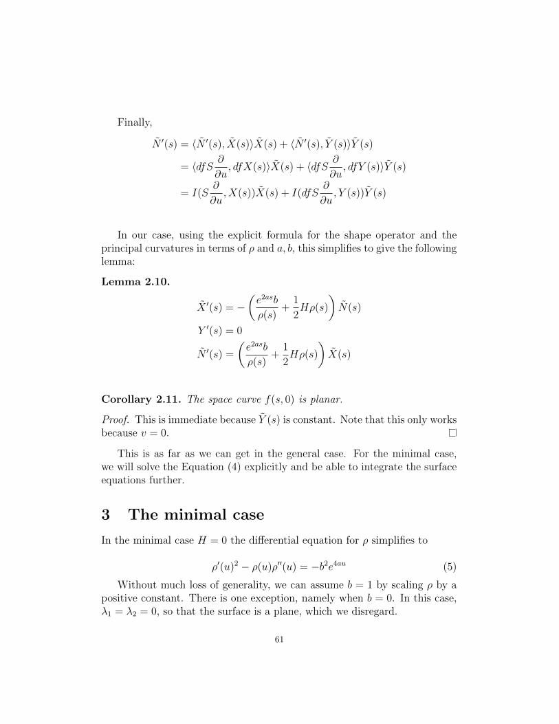
Finally,
N ′(s) = 〈N ′(s), X(s)〉X(s) + 〈N ′(s), Y (s)〉Y (s)
= 〈dfS ∂
∂u, dfX(s)〉X(s) + 〈dfS ∂
∂u, dfY (s)〉Y (s)
= I(S∂
∂u,X(s))X(s) + I(dfS
∂
∂u, Y (s))Y (s)
In our case, using the explicit formula for the shape operator and theprincipal curvatures in terms of ρ and a, b, this simplifies to give the followinglemma:
Lemma 2.10.
X ′(s) = −(e2asb
ρ(s)+
1
2Hρ(s)
)N(s)
Y ′(s) = 0
N ′(s) =
(e2asb
ρ(s)+
1
2Hρ(s)
)X(s)
Corollary 2.11. The space curve f(s, 0) is planar.
Proof. This is immediate because Y (s) is constant. Note that this only worksbecause v = 0.
This is as far as we can get in the general case. For the minimal case,we will solve the Equation (4) explicitly and be able to integrate the surfaceequations further.
3 The minimal case
In the minimal case H = 0 the differential equation for ρ simplifies to
ρ′(u)2 − ρ(u)ρ′′(u) = −b2e4au (5)
Without much loss of generality, we can assume b = 1 by scaling ρ by apositive constant. There is one exception, namely when b = 0. In this case,λ1 = λ2 = 0, so that the surface is a plane, which we disregard.
61
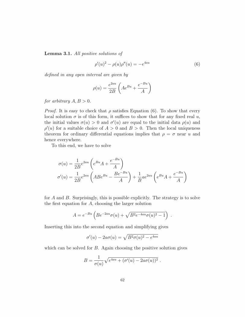
Lemma 3.1. All positive solutions of
ρ′(u)2 − ρ(u)ρ′′(u) = −e4au (6)
defined in any open interval are given by
ρ(u) =e2au
2B
(AeBu +
e−Bu
A
)
for arbitrary A,B > 0.
Proof. It is easy to check that ρ satisfies Equation (6). To show that everylocal solution σ is of this form, it suffices to show that for any fixed real u,the initial values σ(u) > 0 and σ′(u) are equal to the initial data ρ(u) andρ′(u) for a suitable choice of A > 0 and B > 0. Then the local uniquenesstheorem for ordinary differential equations implies that ρ = σ near u andhence everywhere.
To this end, we have to solve
σ(u) =1
2Be2au
(eBuA+
e−Bu
A
)
σ′(u) =1
2Be2au
(ABeBu − Be−Bu
A
)+
1
Bae2au
(eBuA+
e−Bu
A
)
for A and B. Surprisingly, this is possible explicitly. The strategy is to solvethe first equation for A, choosing the larger solution
A = e−Bu(Be−2auσ(u) +
√B2e−4auσ(u)2 − 1
).
Inserting this into the second equation and simplifying gives
σ′(u)− 2aσ(u) =√B2σ(u)2 − e4au
which can be solved for B. Again choosing the positive solution gives
B =1
σ(u)
√e4au + (σ′(u)− 2aσ(u))2 .
62
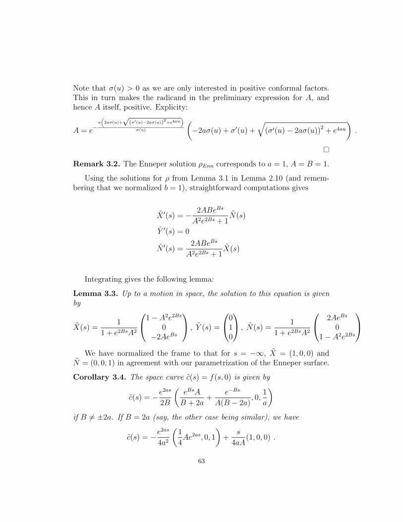
Note that σ(u) > 0 as we are only interested in positive conformal factors.This in turn makes the radicand in the preliminary expression for A, andhence A itself, positive. Explicity:
A = e−u
(2aσ(u)+
√(σ′(u)−2aσ(u))2+e4au
)
σ(u)
(−2aσ(u) + σ′(u) +
√(σ′(u)− 2aσ(u))2 + e4au
).
Remark 3.2. The Enneper solution ρEnn corresponds to a = 1, A = B = 1.
Using the solutions for ρ from Lemma 3.1 in Lemma 2.10 (and remem-bering that we normalized b = 1), straightforward computations gives
X ′(s) = − 2ABeBs
A2e2Bs + 1N(s)
Y ′(s) = 0
N ′(s) =2ABeBs
A2e2Bs + 1X(s)
Integrating gives the following lemma:
Lemma 3.3. Up to a motion in space, the solution to this equation is givenby
X(s) =1
1 + e2BsA2
1− A2e2Bs
0−2AeBs
, Y (s) =
010
, N(s) =
1
1 + e2BsA2
2AeBs
01− A2e2Bs
We have normalized the frame to that for s = −∞, X = (1, 0, 0) andN = (0, 0, 1) in agreement with our parametrization of the Enneper surface.
Corollary 3.4. The space curve c(s) = f(s, 0) is given by
c(s) = −e2as
2B
(eBsA
B + 2a+
e−Bs
A(B − 2a), 0,
1
a
)
if B 6= ±2a. If B = 2a (say, the other case being similar), we have
c(s) = −e2as
4a2
(1
4Ae2as, 0, 1
)+
s
4aA(1, 0, 0) .
63

Proof. This follows by integrating
c′(s) =d
dsf(s, 0)
= I(∂
∂s,X(s))X(s) + I(
∂
∂s, Y (s))Y (s)
= −e2as
2B
(AeBs − e−Bs
A, 0, 2
)
using the previous lemma, and simplifying.
Instead of now integrating the surface equations likewise along the curvess 7→ (u, s) for fixed u, we will use the Bjorling formula [1] to obtain theparametrization more easily.
Recall that given a real analytic curve c : (u1, u2)→ R3 and a real analyticunit normal field N : (u1, u2)→ R3 satisfying 〈c′(u), N(u)〉 = 0, there existsa unique minimal surface containing c and having surface normal N along c,and this surface can be given in a neighborhood of (u1, u2) ⊂ C by
f(z) = Re
(c(z)− i
∫ z
N(w)× c′(w) dw
)
where we write z = u+ iv and have extended c and N to holomorphic mapsinto C3.
In our case, we obtain the explicit formula for f :
f(u, v) =e2au
2B
e−Bu cos((2a−B)v)2aA−AB − AeBu cos((2a+B)v)
2a+Be−Bu sin((2a−B)v)
2aA−AB + AeBu sin((2a+B)v)2a+B
− cos(2av)a
for B 6= 2a, and
f(u, v) =1
4a2
auA− 1
4Ae4au cos(4av)
avA
+ 14Ae4au sin(4av)
−e2au cos(2av)
for B = 2a. Note that in the last case scaling a by a constant and (u, v) bythe reciprocal only scales the surface, so we can as well assume that a = 1 inthis case.
64

The Weierstrass data [1] of these surfaces are particularly simple. Usingz = u+ iv, let (also for B = 2a)
G(z) =1
Ae−Bz and dh = − 1
Be2az dz .
be the Gauss map and height differential of the Weierstrass representationformula
f(z) = Re
∫ z
12(1/G−G)i2(1/G+G)
1
dh .
This gives the surfaces f(u, v) above. This can be verified either byevaluating the integral or by solving the Bjorling integrand c′(z) − iN(z) ×c′(z) for G and dh.
Of particular interest are the cases when B and 2a are integers. Then thesubstitution z = − log(w) changes the Weierstrass data into
G(z) =1
AwB and dh =
1
Bw−2a−1 dw ,
defined on the punctured plane C∗ and being minimal surfaces of finite totalcurvature.
A substitution in the domain of the form w 7→ λw will scale G and dh bypowers of λ, so we can assume without loss of generality that A = 1.
Some of the minimal surfaces we have obtained are described in [3]. Wewill now discuss examples.
Figure 3: The Enneper Surface of order 5
65

In case that B = 2a − 1 ∈ N, we obtain the Enneper surfaces of cyclicsymmetry of order B + 1, see Figure 3. For B = 2a − 1 = 1, we obtain theoriginal Enneper surface.
The planar Enneper surfaces of order n are given by choosing B = n+ 1and 2a = n. See Figure 4 for the cases n = 1 and n = 6. These surfacesfeature an Enneper type end and a planar end. Remarkably, in the non-zeroCMC case, there are only one-ended solutions [5].
(a) order 1 (b) order 6
Figure 4: Planar Enneper surfaces
Other choices of a and B lead to more wildly immersed examples. InFigure 5 we show images of thin annuli u1 < u < u1.
66
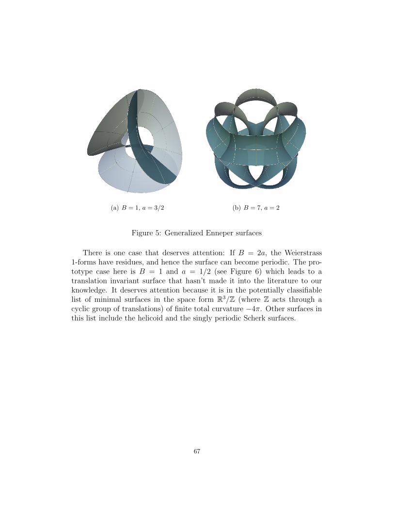
(a) B = 1, a = 3/2 (b) B = 7, a = 2
Figure 5: Generalized Enneper surfaces
There is one case that deserves attention: If B = 2a, the Weierstrass1-forms have residues, and hence the surface can become periodic. The pro-totype case here is B = 1 and a = 1/2 (see Figure 6) which leads to atranslation invariant surface that hasn’t made it into the literature to ourknowledge. It deserves attention because it is in the potentially classifiablelist of minimal surfaces in the space form R3/Z (where Z acts through acyclic group of translations) of finite total curvature −4π. Other surfaces inthis list include the helicoid and the singly periodic Scherk surfaces.
67
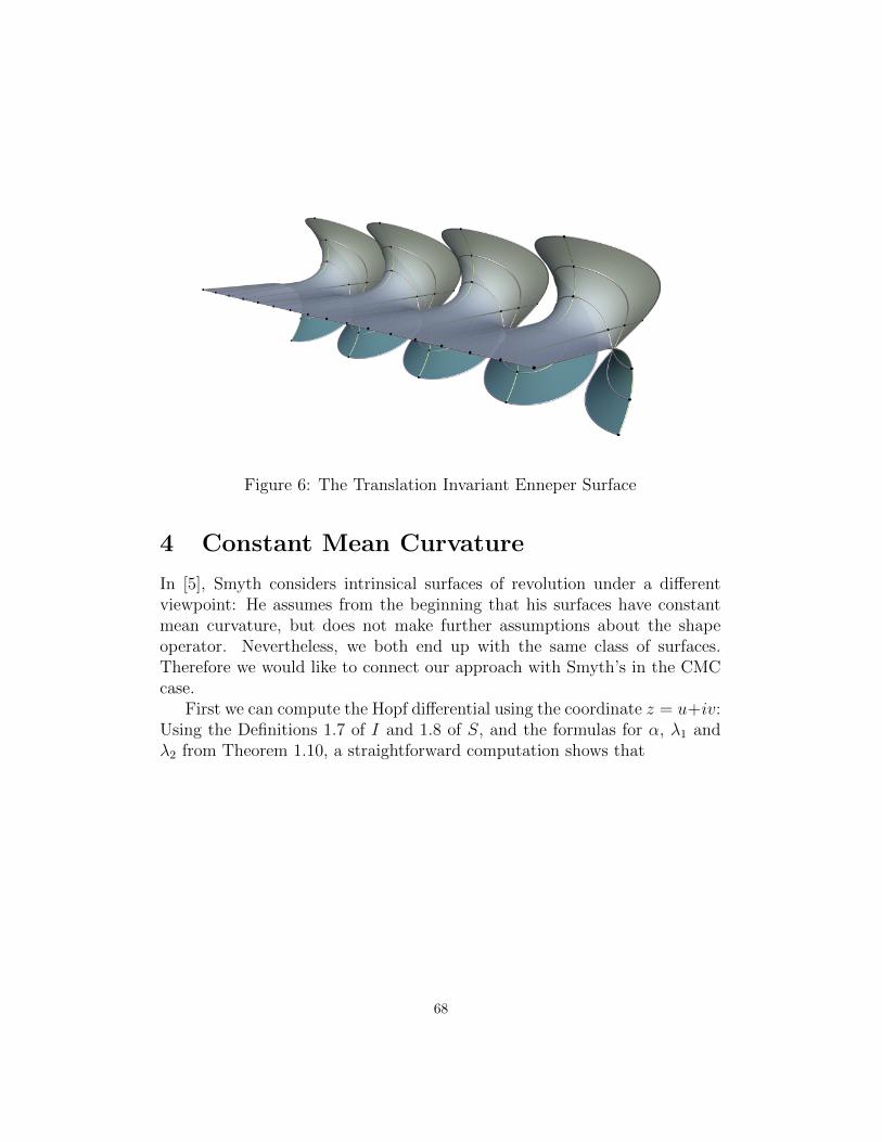
Figure 6: The Translation Invariant Enneper Surface
4 Constant Mean Curvature
In [5], Smyth considers intrinsical surfaces of revolution under a differentviewpoint: He assumes from the beginning that his surfaces have constantmean curvature, but does not make further assumptions about the shapeoperator. Nevertheless, we both end up with the same class of surfaces.Therefore we would like to connect our approach with Smyth’s in the CMCcase.
First we can compute the Hopf differential using the coordinate z = u+iv:Using the Definitions 1.7 of I and 1.8 of S, and the formulas for α, λ1 andλ2 from Theorem 1.10, a straightforward computation shows that
68
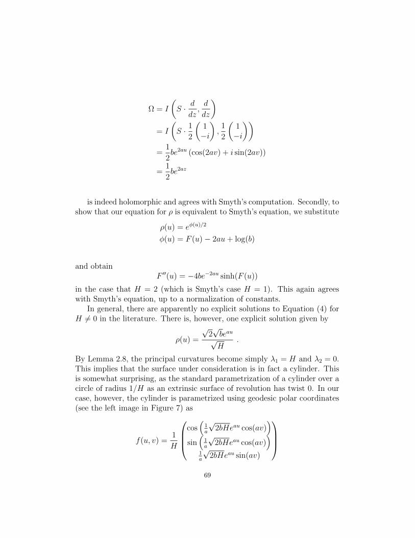
Ω = I
(S · d
dz,d
dz
)
= I
(S · 1
2
(1−i
),1
2
(1−i
))
=1
2be2au (cos(2av) + i sin(2av))
=1
2be2az
is indeed holomorphic and agrees with Smyth’s computation. Secondly, toshow that our equation for ρ is equivalent to Smyth’s equation, we substitute
ρ(u) = eφ(u)/2
φ(u) = F (u)− 2au+ log(b)
and obtainF ′′(u) = −4be−2au sinh(F (u))
in the case that H = 2 (which is Smyth’s case H = 1). This again agreeswith Smyth’s equation, up to a normalization of constants.
In general, there are apparently no explicit solutions to Equation (4) forH 6= 0 in the literature. There is, however, one explicit solution given by
ρ(u) =
√2√beau√H
.
By Lemma 2.8, the principal curvatures become simply λ1 = H and λ2 = 0.This implies that the surface under consideration is in fact a cylinder. Thisis somewhat surprising, as the standard parametrization of a cylinder over acircle of radius 1/H as an extrinsic surface of revolution has twist 0. In ourcase, however, the cylinder is parametrized using geodesic polar coordinates(see the left image in Figure 7) as
f(u, v) =1
H
cos(
1a
√2bHeau cos(av)
)
sin(
1a
√2bHeau cos(av)
)
1a
√2bHeau sin(av)
69
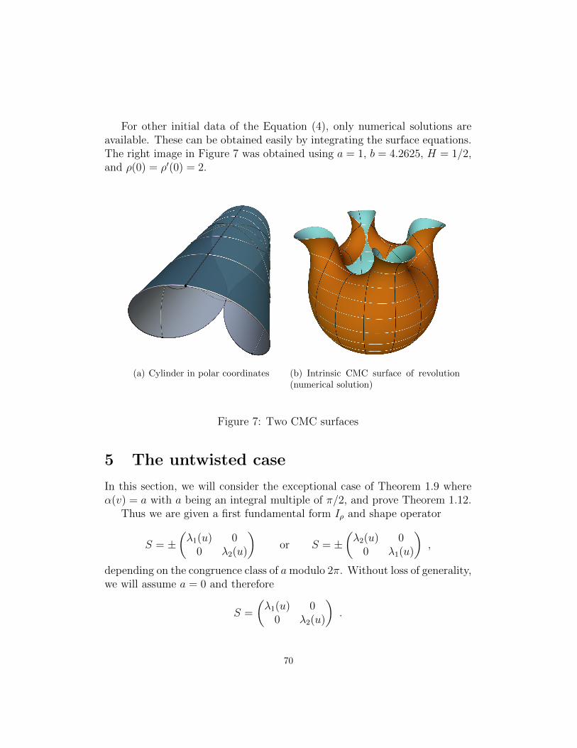
For other initial data of the Equation (4), only numerical solutions areavailable. These can be obtained easily by integrating the surface equations.The right image in Figure 7 was obtained using a = 1, b = 4.2625, H = 1/2,and ρ(0) = ρ′(0) = 2.
(a) Cylinder in polar coordinates (b) Intrinsic CMC surface of revolution(numerical solution)
Figure 7: Two CMC surfaces
5 The untwisted case
In this section, we will consider the exceptional case of Theorem 1.9 whereα(v) = a with a being an integral multiple of π/2, and prove Theorem 1.12.
Thus we are given a first fundamental form Iρ and shape operator
S = ±(λ1(u) 0
0 λ2(u)
)or S = ±
(λ2(u) 0
0 λ1(u)
),
depending on the congruence class of amodulo 2π. Without loss of generality,we will assume a = 0 and therefore
S =
(λ1(u) 0
0 λ2(u)
).
70

The Gauss- and Codazzi equations become
λ1(u)λ2(u) =ρ′(u)2 − ρ(u)ρ′′(u)
ρ(u)4
andρ′
ρ(λ1 − λ2) = λ′2
Eliminating λ1 from the first equation using the second equation leads tothe differential equation
ρ′(u)2 − ρ(u)ρ′′(u)
ρ(u)4= λ2(u)
(λ2(u) +
ρ(u)λ′2(u)
ρ′(u)
)
for λ2. Surprisingly, this equation can be solved explicitly by
λ1(u) =ρ(u)ρ′′(u)− ρ′(u)2
ρ(u)2√c2ρ(u)2 − ρ′(u)2
λ2(u) = −√c2ρ(u)2 − ρ′(u)2
ρ(u)2
for any choice of c that makes the radicand positive.We now show that any untwisted surface is a general surface of revolution.
Recall that typically a surface of revolution is being parametrized as:
f(u, v) = (g(u) cos(v), g(u) sin(v), h(u))
However, by changing the speed of rotation, a surface of revolution canalso be given by
f(u, v) = (g(u) cos(cv), g(u) sin(cv), h(u))
where c is a positive constant.We now show that we can find g and h defined on the interval (u1, u2)
having the first fundamental form and shape operator of the untwisted in-trinsic surface of revolution above, with the rotational speed-up c being theconstant c in Theorem 1.12 introduced above as an integration constant.
The first fundamental form of f is given by:
71
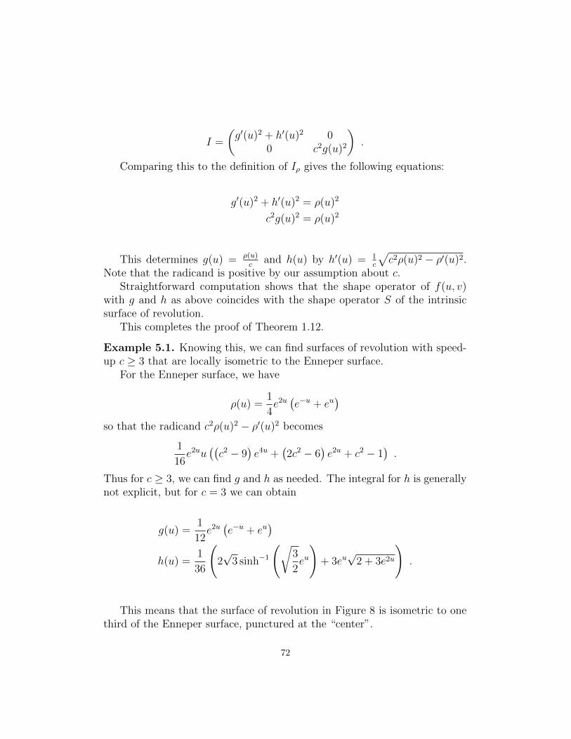
I =
(g′(u)2 + h′(u)2 0
0 c2g(u)2
).
Comparing this to the definition of Iρ gives the following equations:
g′(u)2 + h′(u)2 = ρ(u)2
c2g(u)2 = ρ(u)2
This determines g(u) = ρ(u)c
and h(u) by h′(u) = 1c
√c2ρ(u)2 − ρ′(u)2.
Note that the radicand is positive by our assumption about c.Straightforward computation shows that the shape operator of f(u, v)
with g and h as above coincides with the shape operator S of the intrinsicsurface of revolution.
This completes the proof of Theorem 1.12.
Example 5.1. Knowing this, we can find surfaces of revolution with speed-up c ≥ 3 that are locally isometric to the Enneper surface.
For the Enneper surface, we have
ρ(u) =1
4e2u(e−u + eu
)
so that the radicand c2ρ(u)2 − ρ′(u)2 becomes
1
16e2uu
((c2 − 9
)e4u +
(2c2 − 6
)e2u + c2 − 1
).
Thus for c ≥ 3, we can find g and h as needed. The integral for h is generallynot explicit, but for c = 3 we can obtain
g(u) =1
12e2u(e−u + eu
)
h(u) =1
36
(2√
3 sinh−1(√
3
2eu
)+ 3eu
√2 + 3e2u
).
This means that the surface of revolution in Figure 8 is isometric to onethird of the Enneper surface, punctured at the “center”.
72
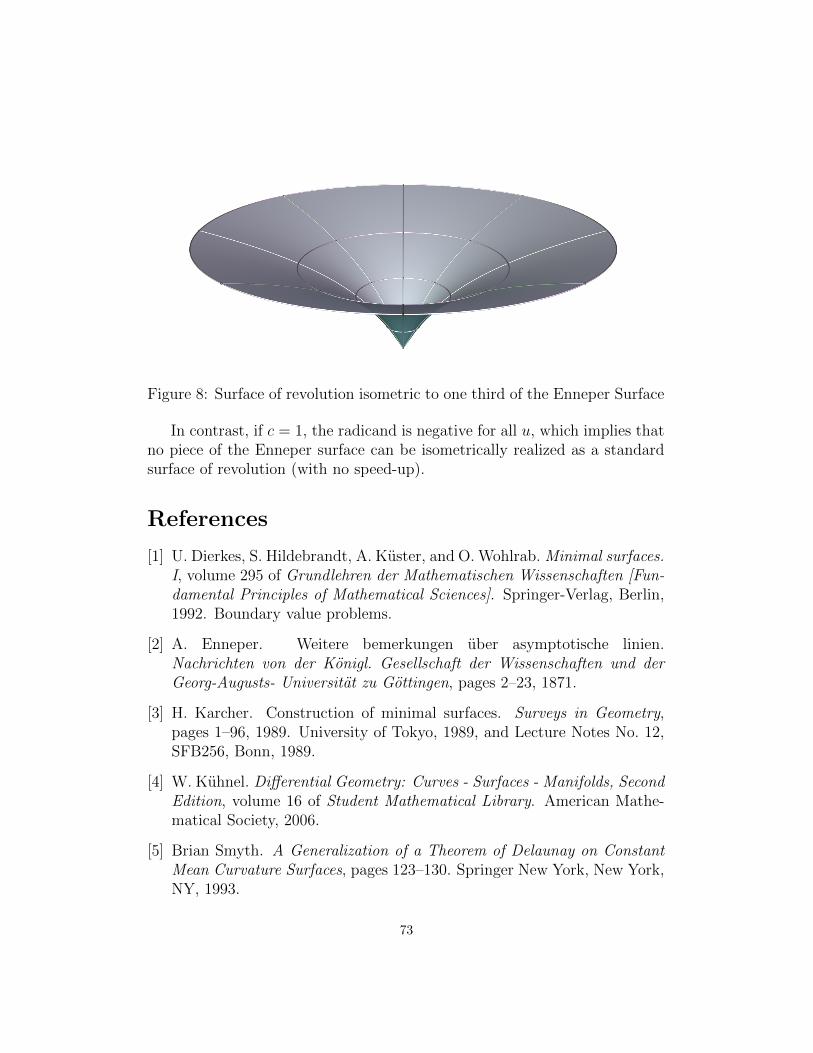
Figure 8: Surface of revolution isometric to one third of the Enneper Surface
In contrast, if c = 1, the radicand is negative for all u, which implies thatno piece of the Enneper surface can be isometrically realized as a standardsurface of revolution (with no speed-up).
References
[1] U. Dierkes, S. Hildebrandt, A. Kuster, and O. Wohlrab. Minimal surfaces.I, volume 295 of Grundlehren der Mathematischen Wissenschaften [Fun-damental Principles of Mathematical Sciences]. Springer-Verlag, Berlin,1992. Boundary value problems.
[2] A. Enneper. Weitere bemerkungen uber asymptotische linien.Nachrichten von der Konigl. Gesellschaft der Wissenschaften und derGeorg-Augusts- Universitat zu Gottingen, pages 2–23, 1871.
[3] H. Karcher. Construction of minimal surfaces. Surveys in Geometry,pages 1–96, 1989. University of Tokyo, 1989, and Lecture Notes No. 12,SFB256, Bonn, 1989.
[4] W. Kuhnel. Differential Geometry: Curves - Surfaces - Manifolds, SecondEdition, volume 16 of Student Mathematical Library. American Mathe-matical Society, 2006.
[5] Brian Smyth. A Generalization of a Theorem of Delaunay on ConstantMean Curvature Surfaces, pages 123–130. Springer New York, New York,NY, 1993.
73

Some Results in the Theory of Elastic Networks
Bat Dejean, Christian GorskiAdvisor: Dylan Thurston
September 14, 2016
Abstract
Elastic networks can be thought of as networks of rubber bandswhich can be stretched in different configurations. Stretching an elas-tic network in Euclidean space has a direct analogy to the study ofresistor networks. However, stretching elastic networks along moregeneral graphs is more complicated. A fundamental question is howto determine when one elastic network is “looser” than another. Oneway to attack this problem is to find the energy of the network as apiecewise-quadratic function of the lengths of the graph in which it isstretched. This is done by examining so-called “train track structures”on the network. We also use geometric methods to prove that an elas-tic tripod is “looser” than any electrically equivalent graph and thatan elastic delta is “tighter” than any electrically equivalent graph. Wegive some generalizations of these results. We give an example of aclass of elastically equivalent graphs and assorted proofs that a tripodis “looser” than the electrically equivalent delta. 1
Introduction
An elastic network, informally speaking, can be thought of as a networkof rubber bands, which has different energies when stretched into differentconfigurations. Mathematically, the act of “stretching” an elastic networkis simply a map (up to some notion of homotopy) from the network to sometarget space. When one stretches an elastic network in a Euclidean space,there is a direct analogy with the well-understood theory of resistor networks(see 2). However, we want to stretch networks in more general spaces; wefocus on the case mapping to trees, but one result generalizes to maps toHadamard spaces.
1This material is based upon work supported by the National Science Foundation underGrant No. DMS-1461061.
74
This paper is largely self-contained, with the exception of a few, morelaborious proofs.
In 1, we give basic definitions and some criteria for harmonicity of maps.In 2 we make explicit the analogy to resistor networks. In 3 we introducetrain track structures and show how they are used to relate the energy of amap to the dimensions of the target tree.
We then use some geometry and the electrical analogy to prove someresults about “looseness.” In 4 we give a proof that tripods are in somesense “minimal-energy” elastic networks for maps to trees and that deltasare “maximal-energy” elastic networks for maps to Hadamard spaces.
As a sort of appendix, we include several other proofs that a tripod is“looser” than its electrically equivalent delta, in the hope that these differentperspectives may be generalized further.
1 Definitions
Throughout this paper, graphs will denote finite 1-dimensional CW com-plexes, with a linear structure on each open edge (1-cell). Maps betweengraphs are continuous maps, which are not required to map vertices to ver-tices. However, we will be focusing on marked graphs, which are graphs witha distinguished finite subset whose points are designated as “marked.” Mapsbetween marked graphs are continuous maps which map marked points tomarked points. Whenever we refer to homotopy, we mean homotopy relativeto marked points; that is, all maps in a given homotopy class are equal whenrestricted to the marked points.
With this in mind, we can make precise the notion of an elastic network.
Definition 1.1. An elastic structure α on a graph Γ is an assignment ofa positive real number to each edge of Γ. We call the real number assignedto an edge e the elasticity of e. The pair (Γ, α) is called an elastic graphor an elastic network. Usually we will use a single symbol, say G, for(Γ, α).
The greater the elasticity of an edge, the “looser” it is. If we treat theelasticities of edges as lengths, the elastic structure induces a metric on thegraph in an obvious way, and this, in turn, induces a measure on the graphin an obvious way.
For most of this paper, we will consider the case of mapping our networkto a graph (usually a tree) with specified edge lengths, which we think of asstretching a network of rubber bands within a network of thin pipes.
75
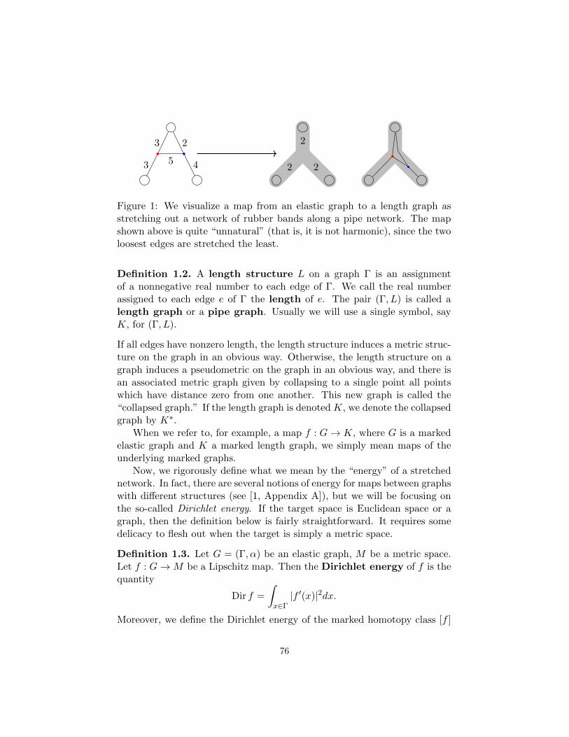
2 2
2
3
3
5
2
4
Figure 1: We visualize a map from an elastic graph to a length graph asstretching out a network of rubber bands along a pipe network. The mapshown above is quite “unnatural” (that is, it is not harmonic), since the twoloosest edges are stretched the least.
Definition 1.2. A length structure L on a graph Γ is an assignmentof a nonnegative real number to each edge of Γ. We call the real numberassigned to each edge e of Γ the length of e. The pair (Γ, L) is called alength graph or a pipe graph. Usually we will use a single symbol, sayK, for (Γ, L).
If all edges have nonzero length, the length structure induces a metric struc-ture on the graph in an obvious way. Otherwise, the length structure on agraph induces a pseudometric on the graph in an obvious way, and there isan associated metric graph given by collapsing to a single point all pointswhich have distance zero from one another. This new graph is called the“collapsed graph.” If the length graph is denoted K, we denote the collapsedgraph by K∗.
When we refer to, for example, a map f : G→ K, where G is a markedelastic graph and K a marked length graph, we simply mean maps of theunderlying marked graphs.
Now, we rigorously define what we mean by the “energy” of a stretchednetwork. In fact, there are several notions of energy for maps between graphswith different structures (see [1, Appendix A]), but we will be focusing onthe so-called Dirichlet energy. If the target space is Euclidean space or agraph, then the definition below is fairly straightforward. It requires somedelicacy to flesh out when the target is simply a metric space.
Definition 1.3. Let G = (Γ, α) be an elastic graph, M be a metric space.Let f : G→M be a Lipschitz map. Then the Dirichlet energy of f is thequantity
Dir f =
∫
x∈Γ|f ′(x)|2dx.
Moreover, we define the Dirichlet energy of the marked homotopy class [f ]
76

to beDir[f ] = inf
g∈[f ]Dir g.
If M is Euclidean space or a graph, then we can define |f ′(x)| to be
limy→x
d(f(x), f(y))
d(x, y),
and this will be defined almost everywhere if f is Lipschitz. More generally,we define |f ′(x)| to be the infimum over all local Lipschitz constants atx, where a local Lipschitz constant at x is just a Lipschitz constant for arestriction of f to a sufficiently small neighborhood of x.
If f minimizes Dirichlet energy within its homotopy class, then |f ′| isconstant on each edge, and for each edge e, we have
|f ′(x)| = `(f(e))
α(e)
for each x ∈ e, where `(f(e)) is the length of the image of e, in a senseappropriate to M . Moreoever, the Dirichlet energy is then
Dir f =∑
e∈Edge(Γ)
`(f(e))2
α(e).
In the case that M is a tree or Euclidean space, this just turns out to bethe distance between the images of the endpoints of e. Also note that, ifthe target is a geodesic space, the images of edges under a harmonic mapare geodesics. We call maps which minimize energy within their homotopyclass harmonic maps. The existence of harmonic maps is not obvious, andis not true in general. A proof for existence in the case of maps into lengthgraphs can be found in Theorem 4 of [1].
We will be dealing primarily with maps into trees in this paper, andthere is a simple criterion (precisely stated in Proposition 5.2 of [1]) whichdetermines whether a map from a marked elastic graph to a length graph isharmonic. We can think of |f ′| as the tension at a point, and then harmonicmaps correspond to a sort of physical equilibrium. Specifically, tensions areconstant at each edge, and “balance” at each vertex. That is, the total ten-sion pulling in any one direction cannot exceed the sums of the (magnitudesof the) tensions pulling in all other directions. This condition is referredto as satisfying the “triangle inequalities.” (See 2.) Notice that if there areonly two directions going out from a point, the inequalities force an equality,
77
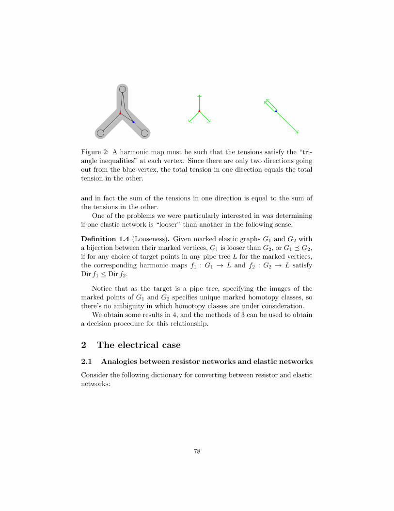
Figure 2: A harmonic map must be such that the tensions satisfy the “tri-angle inequalities” at each vertex. Since there are only two directions goingout from the blue vertex, the total tension in one direction equals the totaltension in the other.
and in fact the sum of the tensions in one direction is equal to the sum ofthe tensions in the other.
One of the problems we were particularly interested in was determiningif one elastic network is “looser” than another in the following sense:
Definition 1.4 (Looseness). Given marked elastic graphs G1 and G2 witha bijection between their marked vertices, G1 is looser than G2, or G1 G2,if for any choice of target points in any pipe tree L for the marked vertices,the corresponding harmonic maps f1 : G1 → L and f2 : G2 → L satisfyDir f1 ≤ Dir f2.
Notice that as the target is a pipe tree, specifying the images of themarked points of G1 and G2 specifies unique marked homotopy classes, sothere’s no ambiguity in which homotopy classes are under consideration.
We obtain some results in 4, and the methods of 3 can be used to obtaina decision procedure for this relationship.
2 The electrical case
2.1 Analogies between resistor networks and elastic networks
Consider the following dictionary for converting between resistor and elasticnetworks:
78

Rubber Band⇔ Resistor
Tension⇔ Current
Position⇔ Voltage
Elasticity⇔ Resistance
Hooke’s Law⇔ Ohm’s Law
Dirichlet energy⇔ Power dissipated
This dictionary translates between Hooke’s law T = Lα and Ohm’s law
I = VR , and the last correspondence is a corollary of the others. This also
allows us to consider elastic graphs as resistor networks: simply let theresistances be the elasticities.
This dictionary is useful for the following reason. If we identify positionwith voltage, f : G→ R1 is harmonic iff it satisfies Kirchhoff’s junction ruleat unmarked nodes: both are equivalent to
∑
e incident to u
f (other node incident to e)− f (u)
α (e)= 0
for every unmarked node u. (Kirchhoff’s loop rule comes for free, asshown in 3.) Thus, under this dictionary, the theories of harmonic maps toR1 and solutions to Kirchhoff’s laws are the same.
0V 10V
0m 10m
Figure 3: That the sum of the red displacements is 0 is Kirchhoff’s looprule, and that the sum of the blue tensions is 0 is Kirchhoff’s junction rule.
This allows us to “import” facts about resistor networks, which arebetter-understood, into the context of harmonic maps to R1.
We can talk about resistor networks being equivalent in the followingsense:
79
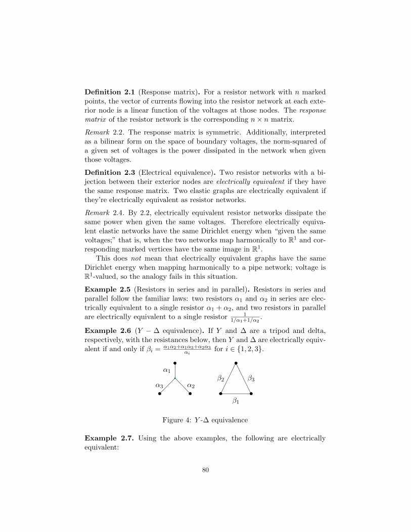
Definition 2.1 (Response matrix). For a resistor network with n markedpoints, the vector of currents flowing into the resistor network at each exte-rior node is a linear function of the voltages at those nodes. The responsematrix of the resistor network is the corresponding n× n matrix.
Remark 2.2. The response matrix is symmetric. Additionally, interpretedas a bilinear form on the space of boundary voltages, the norm-squared ofa given set of voltages is the power dissipated in the network when giventhose voltages.
Definition 2.3 (Electrical equivalence). Two resistor networks with a bi-jection between their exterior nodes are electrically equivalent if they havethe same response matrix. Two elastic graphs are electrically equivalent ifthey’re electrically equivalent as resistor networks.
Remark 2.4. By 2.2, electrically equivalent resistor networks dissipate thesame power when given the same voltages. Therefore electrically equiva-lent elastic networks have the same Dirichlet energy when “given the samevoltages;” that is, when the two networks map harmonically to R1 and cor-responding marked vertices have the same image in R1.
This does not mean that electrically equivalent graphs have the sameDirichlet energy when mapping harmonically to a pipe network; voltage isR1-valued, so the analogy fails in this situation.
Example 2.5 (Resistors in series and in parallel). Resistors in series andparallel follow the familiar laws: two resistors α1 and α2 in series are elec-trically equivalent to a single resistor α1 + α2, and two resistors in parallelare electrically equivalent to a single resistor 1
1/α1+1/α2.
Example 2.6 (Y − ∆ equivalence). If Y and ∆ are a tripod and delta,respectively, with the resistances below, then Y and ∆ are electrically equiv-alent if and only if βi = α1α2+α1α3+α2α3
αifor i ∈ 1, 2, 3.
α3 α2
α1
β1
β3β2
Figure 4: Y -∆ equivalence
Example 2.7. Using the above examples, the following are electricallyequivalent:
80

2
2 7
31
16437
8211
827
115
75
3710
2.2 Classification of networks with three marked vertices
The above “A”-shaped graph was electrically equivalent to a tripod and adelta; is this always true? The answer is no: for example, a network withno edges isn’t equivalent to any tripod or delta. If we include some limit-ing cases corresponding to tripods/deltas with “zero elasticity” or “infiniteelasticity,” the statement is true. More specifically, define the following:
Definition 2.8. A generalized delta is a delta or one of the graphs in 5 anda generalized tripod is a tripod or one of the graphs in 5.
Figure 5: The generalized tripods/deltas
Then we have
Proposition 2.9 (Classification of networks with three marked vertices).Every elastic network with three marked vertices is electrically equivalent toa unique elastic generalized tripod and a unique elastic generalized delta.
Proof. We first show it’s electrically equivalent to a unique generalized ∆.The response matrix of the delta in 4 can be calculated to be
β−1
2 + β−13 −β−1
3 −β−12
−β−13 β−1
1 + β−13 −β−1
1
−β−12 −β−1
1 β−11 + β−1
2
.
With the convention 1∞ = 0, the response matrices of the other gen-
eralized deltas are this matrix in the cases that one or more of the βiis is∞, and all such cases have a generalized delta realizing them. That is, theresponse matrix of a generalized delta is a generic matrix of the above formwith βi ∈ (0,∞], which is a generic symmetric matrix with nonpositive off-diagonal terms and rows summing to 0. It therefore suffices to show everynetwork has such a response matrix.
81
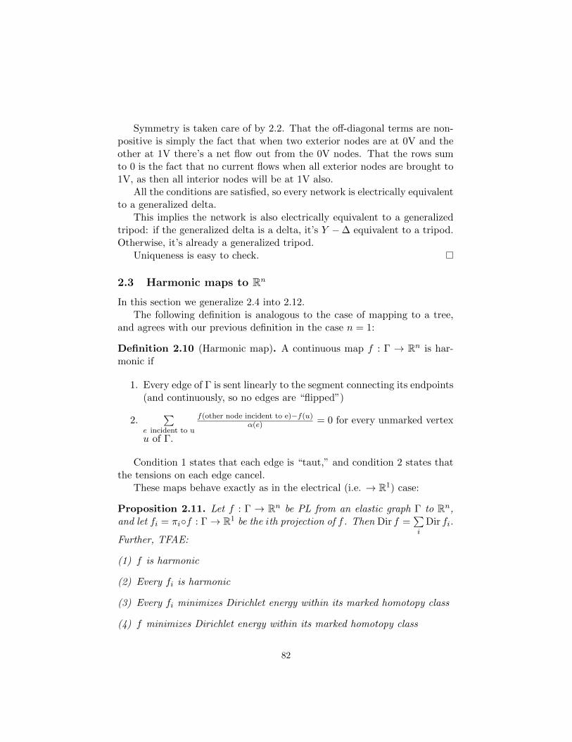
Symmetry is taken care of by 2.2. That the off-diagonal terms are non-positive is simply the fact that when two exterior nodes are at 0V and theother at 1V there’s a net flow out from the 0V nodes. That the rows sumto 0 is the fact that no current flows when all exterior nodes are brought to1V, as then all interior nodes will be at 1V also.
All the conditions are satisfied, so every network is electrically equivalentto a generalized delta.
This implies the network is also electrically equivalent to a generalizedtripod: if the generalized delta is a delta, it’s Y −∆ equivalent to a tripod.Otherwise, it’s already a generalized tripod.
Uniqueness is easy to check.
2.3 Harmonic maps to Rn
In this section we generalize 2.4 into 2.12.The following definition is analogous to the case of mapping to a tree,
and agrees with our previous definition in the case n = 1:
Definition 2.10 (Harmonic map). A continuous map f : Γ → Rn is har-monic if
1. Every edge of Γ is sent linearly to the segment connecting its endpoints(and continuously, so no edges are “flipped”)
2.∑
e incident to u
f(other node incident to e)−f(u)α(e) = 0 for every unmarked vertex
u of Γ.
Condition 1 states that each edge is “taut,” and condition 2 states thatthe tensions on each edge cancel.
These maps behave exactly as in the electrical (i.e. → R1) case:
Proposition 2.11. Let f : Γ → Rn be PL from an elastic graph Γ to Rn,and let fi = πif : Γ→ R1 be the ith projection of f . Then Dir f =
∑i
Dir fi.
Further, TFAE:
(1) f is harmonic
(2) Every fi is harmonic
(3) Every fi minimizes Dirichlet energy within its marked homotopy class
(4) f minimizes Dirichlet energy within its marked homotopy class
82
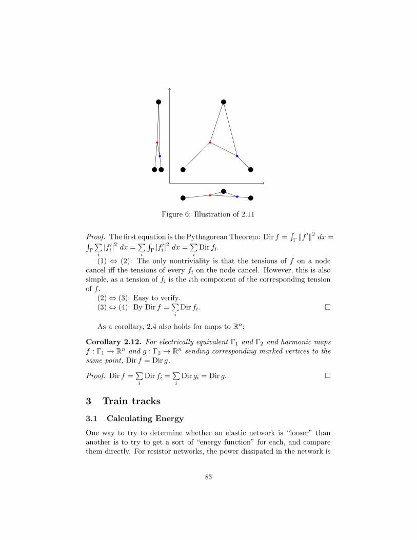
Figure 6: Illustration of 2.11
Proof. The first equation is the Pythagorean Theorem: Dir f =∫
Γ ‖f ′‖2 dx =∫
Γ
∑i|f ′i |2 dx =
∑i
∫Γ |f ′i |
2 dx =∑i
Dir fi.
(1) ⇔ (2): The only nontriviality is that the tensions of f on a nodecancel iff the tensions of every fi on the node cancel. However, this is alsosimple, as a tension of fi is the ith component of the corresponding tensionof f .
(2)⇔ (3): Easy to verify.(3)⇔ (4): By Dir f =
∑i
Dir fi.
As a corollary, 2.4 also holds for maps to Rn:
Corollary 2.12. For electrically equivalent Γ1 and Γ2 and harmonic mapsf : Γ1 → Rn and g : Γ2 → Rn sending corresponding marked vertices to thesame point, Dir f = Dir g.
Proof. Dir f =∑i
Dir fi =∑i
Dir gi = Dir g.
3 Train tracks
3.1 Calculating Energy
One way to try to determine whether an elastic network is “looser” thananother is to try to get a sort of “energy function” for each, and comparethem directly. For resistor networks, the power dissipated in the network is
83

22
2
L3L1
L2
`3`1
`2
`1
`2
`3
Figure 7: We must make combinatorial assumptions about the harmonicmap in order to predict how the stretched lengths relate to the target lengths.On the left, we assume the central elastic vertex is mapped to the centralpipe vertex. On the right, the central elastic vertex has been “pulled up intoan edge.”
just a quadratic function of the boundary voltages. Analogously, we wouldlike to determine the Dirichlet energy of a map from an elastic graph topipe graph as a function of the pipe lengths. More precisely, given a markedelastic graph G, a marked graph Γ, and a marked homotopy class [f ] of mapsfrom G to Γ, there is a harmonic map fL in [f ] for each length structureL on Γ. A length structure on Γ can be viewed as a point in Rn≥0 :=(L1, ..., Ln) ∈ Rn : Li ≥ 0, where n is the number of edges in Γ. What wewant to determine is the energy function E[f ] : Rn≥0 → R, E[f ](L) = Dir fL.
If Γ is topologically a line segment, then the analogy to resistor networkstells us that E[f ] is simply a quadratic function of the length(s) of Γ. More-over, the electrical analogy tells us that we can find the stretched lengths ofG on Γ as a linear function of the length(s) of Γ.
More generally, the stretched lengths of G are a piecewise-linear functionof the target lengths, and E[f ] is piecewise-quadratic. The reason that ourcase is more complicated than the electrical case is that positions are notparametrized by real numbers, and so we have to consider cases where dif-ferent combinations of tensions work with or against each other separately.
Example 3.1. Consider the elastic tripod Y pictured in Figure 7. Wemap it to another marked tripod K, and attempt to calculate the stretchedlengths (`1, `2, `3) of Y as a function of the lengths (L1, L2, L3) of the edgesof K. There are (up to symmetry) two cases to consider. If the central
84

vertex of Y is mapped to the central vertex of K, we clearly have
`1 = L1
`2 = L2
`3 = L3.
If the central vertex of Y is “pulled up” into an edge of K, then we havetwo concerns: the forces at the central vertex must balance, and lengthsmust “match.” That is, the sum of the lengths of the stretched edges in anypath which goes “straight” from one marked vertex to another must equalthe length of the unique geodesic between the marked vertices given by thelength structure on K. So we have
`12
+`32− `2
2= 0
and
`1 + `2 = L1 + L2
`2 + `3 = L2 + L3.
Row reducing then gives the relationship
`1`2`3
=
23
13 −1
313
23
13
−13
13
23
L1
L2
L3
.
From the above example, we see that we need to make some assumptionsabout the combinatorics of the harmonic map to calculate what the rela-tionship between stretched lengths and target lengths is. It turns out therelevant combinatorial information is recorded by “train track structures”on the source graph. These are designed to keep track of which “directions”on the source graph are mapped “in the same direction” on the target.
Intuitively, the “directions” at a point in a graph are simply the direc-tions one can take on a path from the point. Formally, we have the followingdefinition.
Definition 3.2. If Γ is a graph, and x ∈ Γ, then a direction at x is thegerm of a piecewise-linear map (R≥0, 0)→ (Γ, x), considered up to piecewise-linear reparametrization.
85
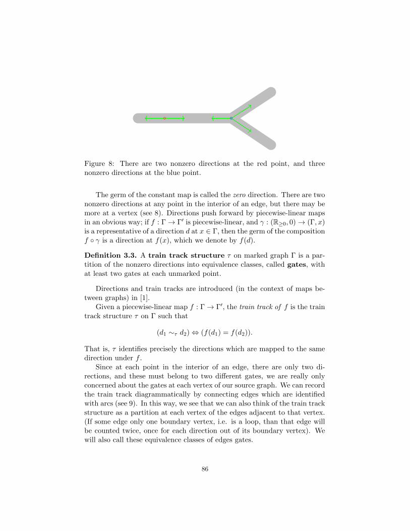
Figure 8: There are two nonzero directions at the red point, and threenonzero directions at the blue point.
The germ of the constant map is called the zero direction. There are twononzero directions at any point in the interior of an edge, but there may bemore at a vertex (see 8). Directions push forward by piecewise-linear mapsin an obvious way; if f : Γ→ Γ′ is piecewise-linear, and γ : (R≥0, 0)→ (Γ, x)is a representative of a direction d at x ∈ Γ, then the germ of the compositionf γ is a direction at f(x), which we denote by f(d).
Definition 3.3. A train track structure τ on marked graph Γ is a par-tition of the nonzero directions into equivalence classes, called gates, withat least two gates at each unmarked point.
Directions and train tracks are introduced (in the context of maps be-tween graphs) in [1].
Given a piecewise-linear map f : Γ→ Γ′, the train track of f is the traintrack structure τ on Γ such that
(d1 ∼τ d2)⇔ (f(d1) = f(d2)).
That is, τ identifies precisely the directions which are mapped to the samedirection under f .
Since at each point in the interior of an edge, there are only two di-rections, and these must belong to two different gates, we are really onlyconcerned about the gates at each vertex of our source graph. We can recordthe train track diagrammatically by connecting edges which are identifiedwith arcs (see 9). In this way, we see that we can also think of the train trackstructure as a partition at each vertex of the edges adjacent to that vertex.(If some edge only one boundary vertex, i.e. is a loop, than that edge willbe counted twice, once for each direction out of its boundary vertex). Wewill also call these equivalence classes of edges gates.
86
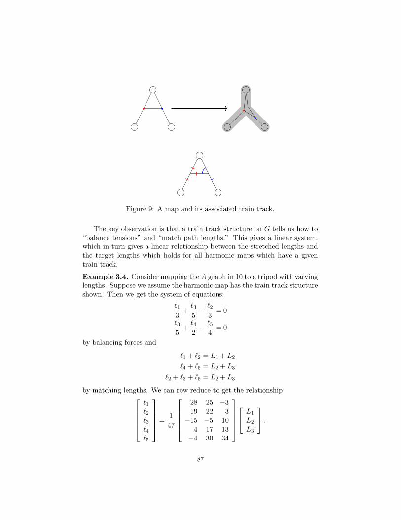
Figure 9: A map and its associated train track.
The key observation is that a train track structure on G tells us how to“balance tensions” and “match path lengths.” This gives a linear system,which in turn gives a linear relationship between the stretched lengths andthe target lengths which holds for all harmonic maps which have a giventrain track.
Example 3.4. Consider mapping the A graph in 10 to a tripod with varyinglengths. Suppose we assume the harmonic map has the train track structureshown. Then we get the system of equations:
`13
+`35− `2
3= 0
`35
+`42− `5
4= 0
by balancing forces and
`1 + `2 = L1 + L2
`4 + `5 = L2 + L3
`2 + `3 + `5 = L2 + L3
by matching lengths. We can row reduce to get the relationship
`1`2`3`4`5
=1
47
28 25 −319 22 3−15 −5 10
4 17 13−4 30 34
L1
L2
L3
.
87
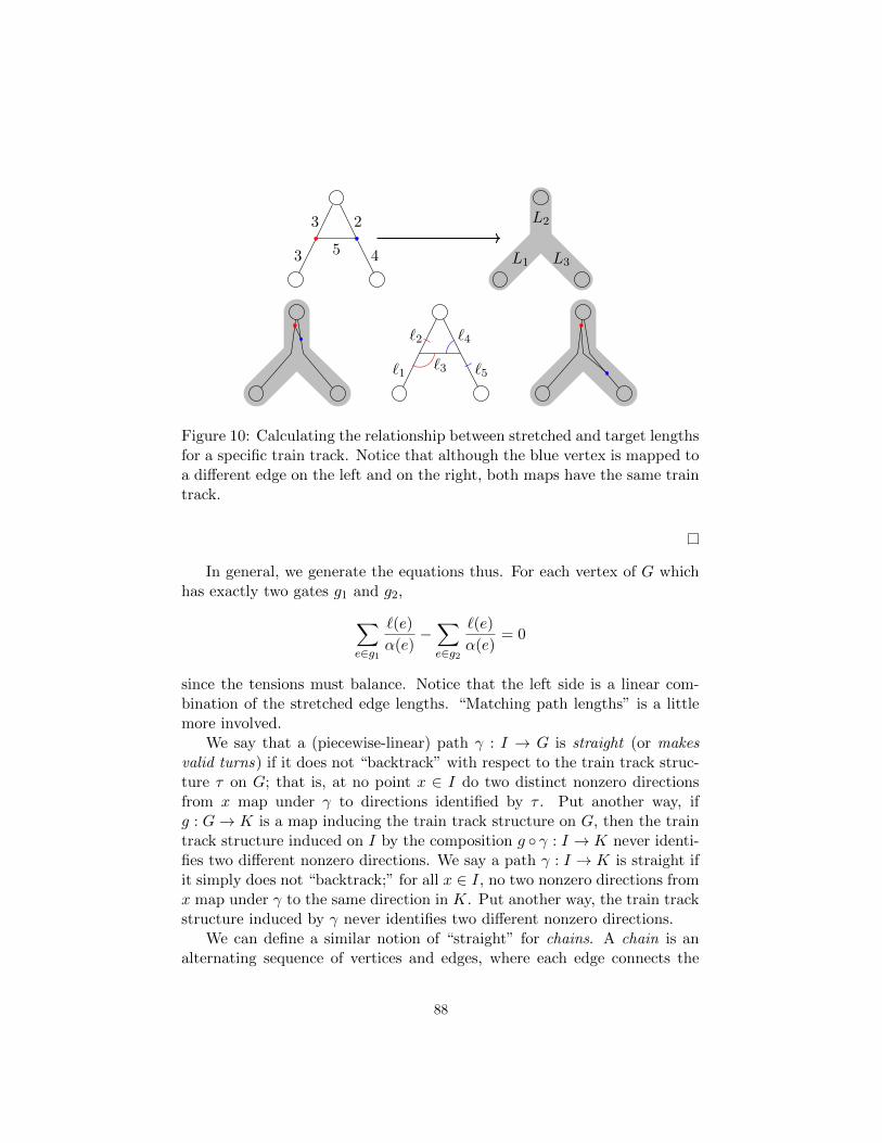
L1
L2
L33
3
5
2
4
`1
`2
`3
`4
`5
Figure 10: Calculating the relationship between stretched and target lengthsfor a specific train track. Notice that although the blue vertex is mapped toa different edge on the left and on the right, both maps have the same traintrack.
In general, we generate the equations thus. For each vertex of G whichhas exactly two gates g1 and g2,
∑
e∈g1
`(e)
α(e)−∑
e∈g2
`(e)
α(e)= 0
since the tensions must balance. Notice that the left side is a linear com-bination of the stretched edge lengths. “Matching path lengths” is a littlemore involved.
We say that a (piecewise-linear) path γ : I → G is straight (or makesvalid turns) if it does not “backtrack” with respect to the train track struc-ture τ on G; that is, at no point x ∈ I do two distinct nonzero directionsfrom x map under γ to directions identified by τ . Put another way, ifg : G→ K is a map inducing the train track structure on G, then the traintrack structure induced on I by the composition g γ : I → K never identi-fies two different nonzero directions. We say a path γ : I → K is straight ifit simply does not “backtrack;” for all x ∈ I, no two nonzero directions fromx map under γ to the same direction in K. Put another way, the train trackstructure induced by γ never identifies two different nonzero directions.
We can define a similar notion of “straight” for chains. A chain is analternating sequence of vertices and edges, where each edge connects the
88
vertices on either side of it. A chain (v0, e1, v1, ..., em, vm) is called straightif it does not “backtrack.” That is, if the chain lies in a graph with a traintrack structure, then we require that ei and ei+1 lie in different gates at vifor each 1 ≤ i ≤ m − 1. If the chain lies in a graph with no train trackstructure, then we must have ei 6= ei+1 for all 1 ≤ i ≤ m− 1, unless ei is aloop whose two directions out from its boundary vertex are not identified.
Given a straight path between vertices, we say a chain parametrizes thepath if some orientation on the edges is such that the path given by concate-nating all the edges in order is homotopic to the original path. Thence, givenour elastic graph G, our length graph K, our homotopy class [f ] : G → K,and a train track structure on τ , we have a way to associate straight chainswith marked endpoints on G to straight chains with marked endpoints onK. Specifically, we associate our chain in G to a (marked) straight pathγ in G which it parametrizes; the homotopy class [f γ] contains (up toPL reparametrization) a unique representative which is straight. (In fact,if g ∈ [f ] induces the train track structure τ on G, then g γ is a straightpath between two marked points in K). We then parametrize the straightpath in [f γ] by a straight chain (v′0, e
′1, v′1, ..., e
′q, v′q). You can think of this
chain as the “image” of our first chain. (We can do a similar process withstraight cycles and straight loops).
Clearly, the total lengths of associated straight chains must match; thefirst chain is a chain of stretched lengths with no backtracking, and thesecond is the path of target lengths along which they are stretched. Thus,having fixed our train track structure, we get
m∑
i=0
`(ei) =
q∑
j=0
L(e′j)
for each straight chain (v0, e1, v1, ..., em, vm) (either with marked endpointsor with v0 = vm) inG and each associated straight chain (v′0, e
′1, v′1, ..., e
′q, v′q).
Notice that the left side a linear combination of stretched lengths and theright is a linear combination of target lengths.
Note that if K is a tree, then any straight chain in K is determinedby its endpoints. This makes computations a lot easier; one simply mustfind straight chains with marked endpoints in G and keep track of wherethe endpoints map in K. (Since K has no cycles, there will be no straightcycles in G if τ is actually induced by a map to K). This method is fairlystraightforward to program; in fact, we used this method to write a programgiving the relationship between stretched lengths and target lengths and theenergy function for maps from 3-marked elastic graphs to a tripod.
89
In all of our experiments mapping different 3-marked networks to thetripod, the system produced had a unique solution for each assignment oftarget lengths (although most of the time there were redundant equations).We do not yet have a proof that these systems of equations have uniquesolutions, but we suspect that they do in the case that K is a tree.
Assuming the systems are sufficiently determined, then for a specifiedtrain track τ , by row-reducing our system, we get a matrix we get a matrixT such that
`1...`N
= T
L1...Ln
.
If
A =
α1
. . .
αN
is the diagonal matrix of the elasticities of the source graph, then the Dirich-let energy of a map is
Dir g =[`1 · · · `N
]A
`1...`N
=
T
L1...Ln
t
A
L1...Ln
=[L1 · · · Ln
]M
L1...Ln
,
where M = T tAT . Thus, we have explicitly obtained a piece of our energyfunction.
3.2 Regions of Validity
In order to get our system of equations, we had to assume that the har-monic representative of [f ] had a specific train track structure. However,the assignment of target lengths (L1, ..., Ln) already determines the har-monic representative(s), which in turn determines a train track structure(or structures) which may differ from our assumption. Therefore, we wantto determine which assignments of target lengths correspond to which traintrack structures, and thence how the “pieces” of our piecewise-quadraticenergy function are shaped and arranged.
90
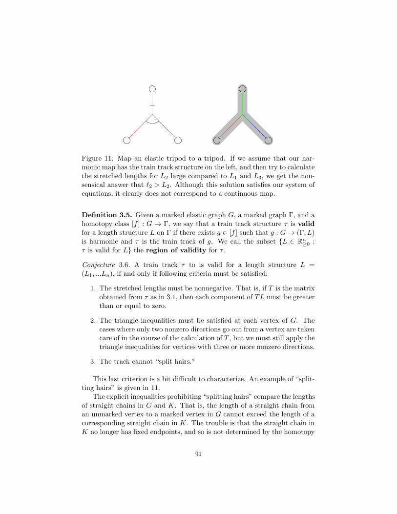
Figure 11: Map an elastic tripod to a tripod. If we assume that our har-monic map has the train track structure on the left, and then try to calculatethe stretched lengths for L2 large compared to L1 and L3, we get the non-sensical answer that `2 > L2. Although this solution satisfies our system ofequations, it clearly does not correspond to a continuous map.
Definition 3.5. Given a marked elastic graph G, a marked graph Γ, and ahomotopy class [f ] : G → Γ, we say that a train track structure τ is validfor a length structure L on Γ if there exists g ∈ [f ] such that g : G→ (Γ, L)is harmonic and τ is the train track of g. We call the subset L ∈ Rn≥0 :τ is valid for L the region of validity for τ .
Conjecture 3.6. A train track τ to is valid for a length structure L =(L1, ...Ln), if and only if following criteria must be satisfied:
1. The stretched lengths must be nonnegative. That is, if T is the matrixobtained from τ as in 3.1, then each component of TL must be greaterthan or equal to zero.
2. The triangle inequalities must be satisfied at each vertex of G. Thecases where only two nonzero directions go out from a vertex are takencare of in the course of the calculation of T , but we must still apply thetriangle inequalities for vertices with three or more nonzero directions.
3. The track cannot “split hairs.”
This last criterion is a bit difficult to characterize. An example of “split-ting hairs” is given in 11.
The explicit inequalities prohibiting “splitting hairs” compare the lengthsof straight chains in G and K. That is, the length of a straight chain froman unmarked vertex to a marked vertex in G cannot exceed the length of acorresponding straight chain in K. The trouble is that the straight chain inK no longer has fixed endpoints, and so is not determined by the homotopy
91

class. Instead, the corresponding chain is the smallest that contains theimage of the original under any map which has the given train track.
Clearly, the criteria in 3.6 are necessary for a train track to be valid.The conjecture is that they are sufficient. More work needs to be done toprove this, and perhaps find a better characterization of the last condition.
So long as these conditions are the correct ones, we then know that theregions of validity are polyhedra. That is, they are intersections Euclideanhalf-spaces. This is because each of the conditions manifests itself as asystem of linear inequalities of the stretched lengths, which, through ourcalculated relationship T from 3.1 are transformed into linear inequalitiesof the target lengths. (The solution sets of linear inequalities are, of course,polyhedra). Moreover, we know that the regions of validity are cones (thatis, invariant under positive scalar multiplication), since scaling up the targetlengths uniformly will not change the combinatorics of the harmonic map.Alternatively, one may note that the inequalities correspond to whethersome linear transformation maps into the first quadrant.
Since the regions of validity are cones, we can get all the information weneed about them from their projection onto the standard (n − 1)-simplex(the subset on which the sum of all the target lengths is 1). This is especiallyconvenient, since then for maps to a tripod, we have a clear 2-dimensionalrepresentation of the regions of validity.
Using code written by the authors, as well as code written by AndrewHenderson and code written by Dylan Thurston, we were able to experi-mentally determine and plot the regions of validity for different train trackstructures on some maps into tripods. These are presented in 12 and 13.
Understanding regions of validity allows one to understand the globalstructure of the energy functions of maps between graphs. For each n,there are only finitely many trees with n boundary vertices, and so we canunderstand the energies of maps from a fixed elastic graph with n markedpoints into a tree by examining finitely many homotopy classes of maps andfinitely many train track structures. This would give a decision procedureto check whether one network is looser than another directly; we just check–on finitely many sufficiently small regions of Rn≥0–whether one quadraticfunction is greater than another. Geometric approaches to getting resultsabout looseness are given in the next section.
92

Figure 12: On the left, we have pictured experimentally determined regionsof validity for maps from an A graph with uniform elasticities graph into thetripod. The different colors represent different train track structures on A.On the right, we have all the different train track structures that will occurfor a map from any elastic A to the tripod. Edges are drawn between traintrack structures which are in some sense similar. We see that this graphcorresponds nicely to the regions on the left.
1
1 1
1
11
1 1 1
1 1
1
12
1 1
Figure 13: We map the elastic (“M”) graphs shown in the top row to thetripod and plot the regions of validity of the train tracks that appear. For theuniformly elastic M , only 9 distinct train tracks are valid in a 3-dimensionalregion. When we break the symmetry as in the graph on the right, 5 moreregions appear. If we try to make a graph of all possible train track structure,as in 12, we get a much larger graph that does not correspond nicely to eitherof these, and, in fact, does not embed nicely into the plane. Further workmust be done to characterize how regions of validity collapse and evolve aswe vary elasticities on the source.
93
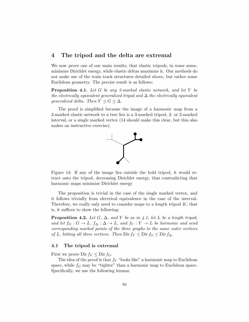
4 The tripod and the delta are extremal
We now prove one of our main results, that elastic tripods, in some sense,minimize Dirichlet energy, while elastic deltas maximize it. Our methods donot make use of the train track structures detailed above, but rather someEuclidean geometry. The precise result is as follows:
Proposition 4.1. Let G be any 3-marked elastic network, and let Y bethe electrically equivalent generalized tripod and ∆ the electrically equivalentgeneralized delta. Then Y G ∆.
The proof is simplified because the image of a harmonic map from a3-marked elastic network to a tree lies is a 3-marked tripod, 2- or 3-markedinterval, or a single marked vertex (14 should make this clear, but this alsomakes an instructive exercise).
Figure 14: If any of the image lies outside the bold tripod, it would re-tract onto the tripod, decreasing Dirichlet energy, thus contradicting thatharmonic maps minimize Dirichlet energy
The proposition is trivial in the case of the single marked vertex, andit follows trivially from electrical equivalence in the case of the interval.Therefore, we really only need to consider maps to a length tripod K; thatis, it suffices to show the following:
Proposition 4.2. Let G, ∆, and Y be as in 4.1, let L be a length tripod,and let fG : G → L, f∆ : ∆ → L, and fY : Y → L be harmonic and sendcorresponding marked points of the three graphs to the same outer verticesof L, hitting all three vertices. Then Dir fY ≤ Dir fG ≤ Dir f∆.
4.1 The tripod is extremal
First we prove Dir fY ≤ Dir fG.The idea of the proof is that fY “looks like” a harmonic map to Euclidean
space, while fG may be “tighter” than a harmonic map to Euclidean space.Specifically, we use the following lemma:
94
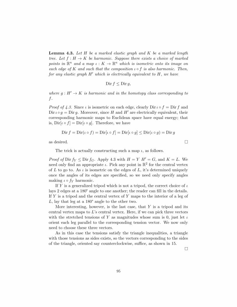
Lemma 4.3. Let H be a marked elastic graph and K be a marked lengthtree. Let f : H → K be harmonic. Suppose there exists a choice of markedpoints in Rn and a map ι : K → Rn which is isometric onto its image oneach edge of K and such that the composition ι f is also harmonic. Then,for any elastic graph H ′ which is electrically equivalent to H, we have
Dir f ≤ Dir g,
where g : H ′ → K is harmonic and in the homotopy class corresponding tof .
Proof of 4.3. Since ι is isometric on each edge, clearly Dir ι f = Dir f andDir ι g = Dir g. Moreover, since H and H ′ are electrically equivalent, theircorresponding harmonic maps to Euclidean space have equal energy; thatis, Dir[ι f ] = Dir[ι g]. Therefore, we have
Dir f = Dir(ι f) = Dir[ι f ] = Dir[ι g] ≤ Dir(ι g) = Dir g
as desired.
The trick is actually constructing such a map ι, as follows.
Proof of Dir fY ≤ Dir fG. Apply 4.3 with H = Y H ′ = G, and K = L. Weneed only find an appropriate ι. Pick any point in R2 for the central vertexof L to go to. As ι is isometric on the edges of L, it’s determined uniquelyonce the angles of its edges are specified, so we need only specify anglesmaking ι fY harmonic.
If Y is a generalized tripod which is not a tripod, the correct choice of ιlays 2 edges at a 180° angle to one another; the reader can fill in the details.If Y is a tripod and the central vertex of Y maps to the interior of a leg ofL, lay that leg at a 180° angle to the other two.
More interesting, however, is the last case, that Y is a tripod and itscentral vertex maps to L’s central vertex. Here, if we can pick three vectorswith the stretched tensions of Y as magnitudes whose sum is 0, just let ιorient each leg parallel to the corresponding tension vector. We now onlyneed to choose these three vectors.
As in this case the tensions satisfy the triangle inequalities, a trianglewith those tensions as sides exists, so the vectors corresponding to the sidesof the triangle, oriented say counterclockwise, suffice, as shown in 15.
95
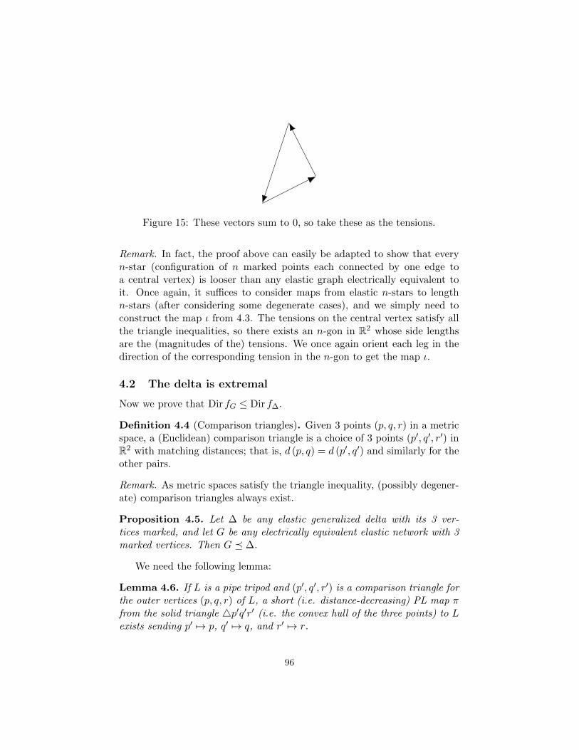
Figure 15: These vectors sum to 0, so take these as the tensions.
Remark. In fact, the proof above can easily be adapted to show that everyn-star (configuration of n marked points each connected by one edge toa central vertex) is looser than any elastic graph electrically equivalent toit. Once again, it suffices to consider maps from elastic n-stars to lengthn-stars (after considering some degenerate cases), and we simply need toconstruct the map ι from 4.3. The tensions on the central vertex satisfy allthe triangle inequalities, so there exists an n-gon in R2 whose side lengthsare the (magnitudes of the) tensions. We once again orient each leg in thedirection of the corresponding tension in the n-gon to get the map ι.
4.2 The delta is extremal
Now we prove that Dir fG ≤ Dir f∆.
Definition 4.4 (Comparison triangles). Given 3 points (p, q, r) in a metricspace, a (Euclidean) comparison triangle is a choice of 3 points (p′, q′, r′) inR2 with matching distances; that is, d (p, q) = d (p′, q′) and similarly for theother pairs.
Remark. As metric spaces satisfy the triangle inequality, (possibly degener-ate) comparison triangles always exist.
Proposition 4.5. Let ∆ be any elastic generalized delta with its 3 ver-tices marked, and let G be any electrically equivalent elastic network with 3marked vertices. Then G ∆.
We need the following lemma:
Lemma 4.6. If L is a pipe tripod and (p′, q′, r′) is a comparison triangle forthe outer vertices (p, q, r) of L, a short (i.e. distance-decreasing) PL map πfrom the solid triangle 4p′q′r′ (i.e. the convex hull of the three points) to Lexists sending p′ 7→ p, q′ 7→ q, and r′ 7→ r.
96

Proof of 4.6. A map from the boundary of the comparison triangle (that is,the union of the segments connecting two of the comparison points) to Lexists which is isometric on each edge: send segment p′q′ isometrically tothe geodesic pq, and so on. Informally, we can think of this map as addinga hinge to the comparison triangle at each of its vertices and each of thethree preimages of the central vertex, and then “collapsing” the triangle, asshown in 16.
3
452 1
3
Figure 16: A comparison triangle collapsing onto its tripod
Notice that the pink preimages of the central vertex are the points wherethe incircle of 4p′q′r′ meets the triangle; this can be seen, for instance, bythe fact that only one choice of three pink points satisfies the congruencesin the first triangle of figure 1 and the points where the incircle meets thetriangle also satisfy them.
We can therefore extend this collapse to the entire solid triangle: sub-divide the triangle into 3 via its angle bisectors and orthogonally projecteach subtriangle onto its corresponding side as shown in 17 before collaps-ing. Notice this is well-defined on the angle bisectors: no matter which sidewe project onto to resolve the ambiguity, the image in the final tripod is thesame. Call the extension π.
p′ r′
q′
p r
q
Figure 17: The extended map π
Now π is short, as desired: the pullback metric (in the sense of differentialgeometry) from the tripod, which is defined a.e., is simply the appropriateorthogonal projection of the Euclidean metric, and so measures distances no
97
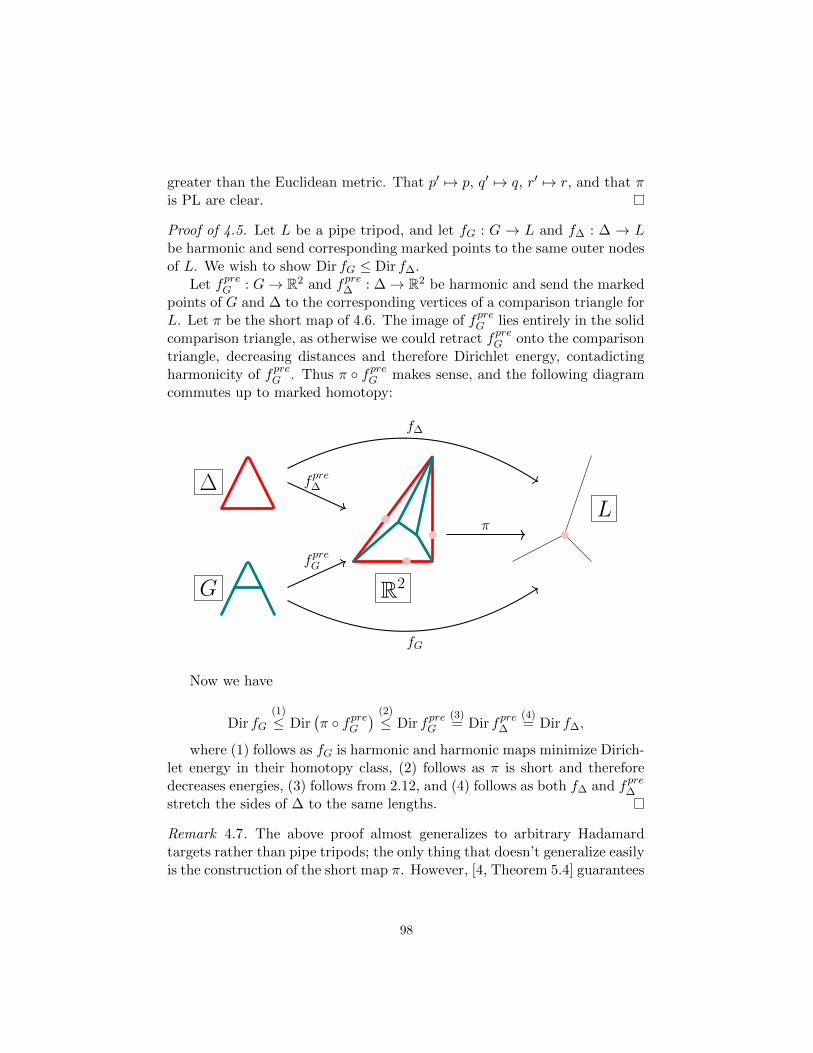
greater than the Euclidean metric. That p′ 7→ p, q′ 7→ q, r′ 7→ r, and that πis PL are clear.
Proof of 4.5. Let L be a pipe tripod, and let fG : G → L and f∆ : ∆ → Lbe harmonic and send corresponding marked points to the same outer nodesof L. We wish to show Dir fG ≤ Dir f∆.
Let fpreG : G→ R2 and fpre∆ : ∆→ R2 be harmonic and send the markedpoints of G and ∆ to the corresponding vertices of a comparison triangle forL. Let π be the short map of 4.6. The image of fpreG lies entirely in the solidcomparison triangle, as otherwise we could retract fpreG onto the comparisontriangle, decreasing distances and therefore Dirichlet energy, contadictingharmonicity of fpreG . Thus π fpreG makes sense, and the following diagramcommutes up to marked homotopy:
∆
G R2
L
fpre∆
fpreG
π
f∆
fG
Now we have
Dir fG(1)
≤ Dir(π fpreG
) (2)
≤ Dir fpreG
(3)= Dir fpre∆
(4)= Dir f∆,
where (1) follows as fG is harmonic and harmonic maps minimize Dirich-let energy in their homotopy class, (2) follows as π is short and thereforedecreases energies, (3) follows from 2.12, and (4) follows as both f∆ and fpre∆
stretch the sides of ∆ to the same lengths.
Remark 4.7. The above proof almost generalizes to arbitrary Hadamardtargets rather than pipe tripods; the only thing that doesn’t generalize easilyis the construction of the short map π. However, [4, Theorem 5.4] guarantees
98
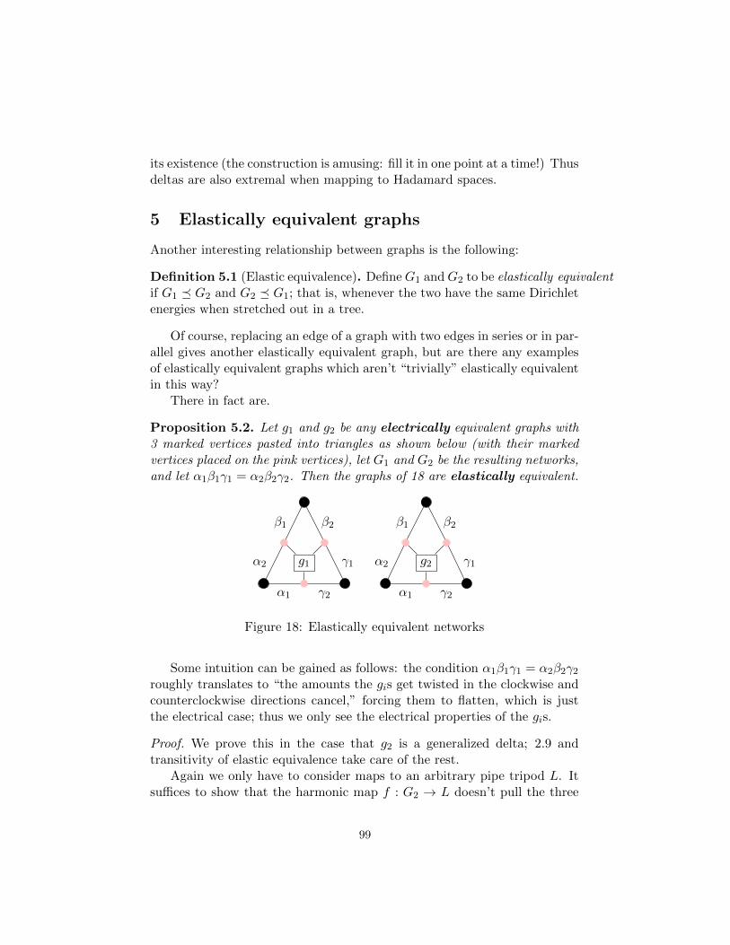
its existence (the construction is amusing: fill it in one point at a time!) Thusdeltas are also extremal when mapping to Hadamard spaces.
5 Elastically equivalent graphs
Another interesting relationship between graphs is the following:
Definition 5.1 (Elastic equivalence). DefineG1 andG2 to be elastically equivalentif G1 G2 and G2 G1; that is, whenever the two have the same Dirichletenergies when stretched out in a tree.
Of course, replacing an edge of a graph with two edges in series or in par-allel gives another elastically equivalent graph, but are there any examplesof elastically equivalent graphs which aren’t “trivially” elastically equivalentin this way?
There in fact are.
Proposition 5.2. Let g1 and g2 be any electrically equivalent graphs with3 marked vertices pasted into triangles as shown below (with their markedvertices placed on the pink vertices), let G1 and G2 be the resulting networks,and let α1β1γ1 = α2β2γ2. Then the graphs of 18 are elastically equivalent.
α1 γ2
γ1
β2β1
α2 g1
α1 γ2
γ1
β2β1
α2 g2
Figure 18: Elastically equivalent networks
Some intuition can be gained as follows: the condition α1β1γ1 = α2β2γ2
roughly translates to “the amounts the gis get twisted in the clockwise andcounterclockwise directions cancel,” forcing them to flatten, which is justthe electrical case; thus we only see the electrical properties of the gis.
Proof. We prove this in the case that g2 is a generalized delta; 2.9 andtransitivity of elastic equivalence take care of the rest.
Again we only have to consider maps to an arbitrary pipe tripod L. Itsuffices to show that the harmonic map f : G2 → L doesn’t pull the three
99
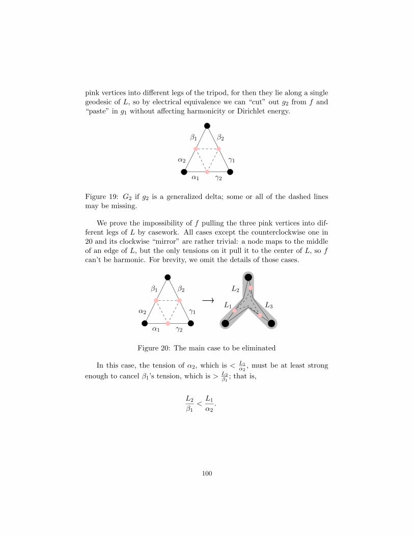
pink vertices into different legs of the tripod, for then they lie along a singlegeodesic of L, so by electrical equivalence we can “cut” out g2 from f and“paste” in g1 without affecting harmonicity or Dirichlet energy.
α1 γ2
γ1
β2β1
α2
Figure 19: G2 if g2 is a generalized delta; some or all of the dashed linesmay be missing.
We prove the impossibility of f pulling the three pink vertices into dif-ferent legs of L by casework. All cases except the counterclockwise one in20 and its clockwise “mirror” are rather trivial: a node maps to the middleof an edge of L, but the only tensions on it pull it to the center of L, so fcan’t be harmonic. For brevity, we omit the details of those cases.
L1 L3
L2
α1 γ2
γ1
β2β1
α2
Figure 20: The main case to be eliminated
In this case, the tension of α2, which is < L1α2
, must be at least strong
enough to cancel β1’s tension, which is > L2β1
; that is,
L2
β1<L1
α2.
100
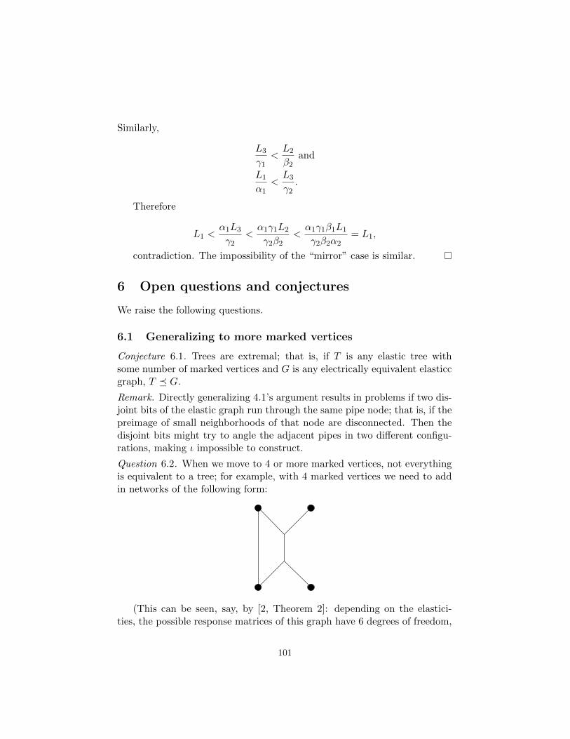
Similarly,
L3
γ1<L2
β2and
L1
α1<L3
γ2.
Therefore
L1 <α1L3
γ2<α1γ1L2
γ2β2<α1γ1β1L1
γ2β2α2= L1,
contradiction. The impossibility of the “mirror” case is similar.
6 Open questions and conjectures
We raise the following questions.
6.1 Generalizing to more marked vertices
Conjecture 6.1. Trees are extremal; that is, if T is any elastic tree withsome number of marked vertices and G is any electrically equivalent elasticcgraph, T G.
Remark. Directly generalizing 4.1’s argument results in problems if two dis-joint bits of the elastic graph run through the same pipe node; that is, if thepreimage of small neighborhoods of that node are disconnected. Then thedisjoint bits might try to angle the adjacent pipes in two different configu-rations, making ι impossible to construct.
Question 6.2. When we move to 4 or more marked vertices, not everythingis equivalent to a tree; for example, with 4 marked vertices we need to addin networks of the following form:
(This can be seen, say, by [2, Theorem 2]: depending on the elastici-ties, the possible response matrices of this graph have 6 degrees of freedom,
101
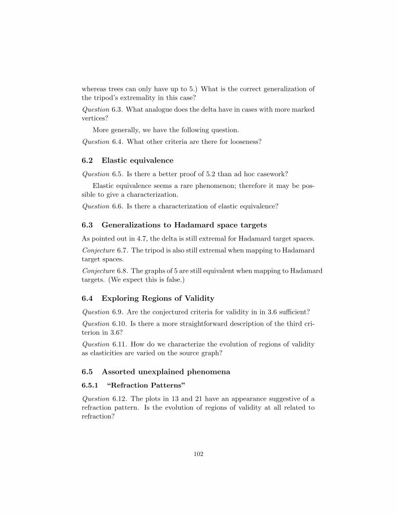
whereas trees can only have up to 5.) What is the correct generalization ofthe tripod’s extremality in this case?
Question 6.3. What analogue does the delta have in cases with more markedvertices?
More generally, we have the following question.
Question 6.4. What other criteria are there for looseness?
6.2 Elastic equivalence
Question 6.5. Is there a better proof of 5.2 than ad hoc casework?
Elastic equivalence seems a rare phenomenon; therefore it may be pos-sible to give a characterization.
Question 6.6. Is there a characterization of elastic equivalence?
6.3 Generalizations to Hadamard space targets
As pointed out in 4.7, the delta is still extremal for Hadamard target spaces.
Conjecture 6.7. The tripod is also still extremal when mapping to Hadamardtarget spaces.
Conjecture 6.8. The graphs of 5 are still equivalent when mapping to Hadamardtargets. (We expect this is false.)
6.4 Exploring Regions of Validity
Question 6.9. Are the conjectured criteria for validity in in 3.6 sufficient?
Question 6.10. Is there a more straightforward description of the third cri-terion in 3.6?
Question 6.11. How do we characterize the evolution of regions of validityas elasticities are varied on the source graph?
6.5 Assorted unexplained phenomena
6.5.1 “Refraction Patterns”
Question 6.12. The plots in 13 and 21 have an appearance suggestive of arefraction pattern. Is the evolution of regions of validity at all related torefraction?
102
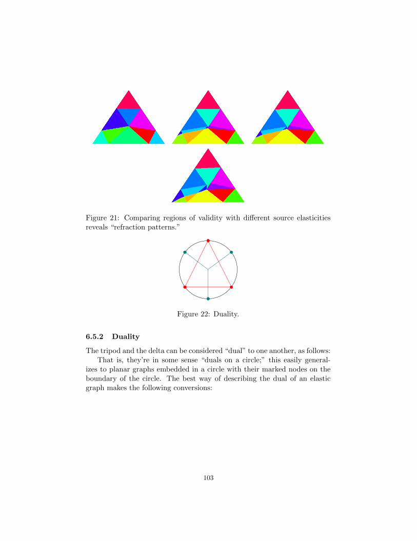
Figure 21: Comparing regions of validity with different source elasticitiesreveals “refraction patterns.”
Figure 22: Duality.
6.5.2 Duality
The tripod and the delta can be considered “dual” to one another, as follows:That is, they’re in some sense “duals on a circle;” this easily general-
izes to planar graphs embedded in a circle with their marked nodes on theboundary of the circle. The best way of describing the dual of an elasticgraph makes the following conversions:
103
Tension⇒ Length
Length⇒ Tension
Elasticity⇒ 1
Elasticity
Hooke’s Law⇒ Hooke’s Law
Dirichlet energy⇒ Dirichlet energy
The most remarkable things, however, are the following:
Kirchoff’s loop rule⇒ Kirchoff’s junction rule
Kirchoff’s junction rule⇒ Kirchoff’s loop rule
This has been explored for resistor networks; for example, in [3, Section3] the electrical case with 2 marked vertices is examined.
Due to a number of suggestive facts, we believe this should generalizesomehow to harmonic maps from elastic graphs to pipe graphs. Firstly, thetriangle inequality condition for harmonicity is exactly dual to the metrictriangle inequality between the endpoints of a pipe tripod, generalizing theswap between Kirchoff’s laws in the electrical case. In addition, a numberof matrices that seemed related to duality (from calculations of how dualityshould behave) appeared in other calculations. Even the two triangles inthe proofs of 4 are dual to one another!
A full description of duality seems elusive, however. We hope futurework can shed some light on this.
A Assorted proofs that Y ∆
Over the course of our research, we found several proofs of the followingproposition:
Proposition A.1. Let Y be an elastic tripod, let ∆ be an electrically equiv-alent delta, and let K be a length tripod. If f : Y → K is harmonic,and g : ∆ → K is harmonic in the corresponding homotopy class, thenDir f ≤ Dir g.
This is, of course, implied by our main results in 4. However, it maybe fruitful to examine the different proofs we found and search for gen-eralizations. Therefore, we include several proofs (sometimes under moreassumptions) of A.1 below.
104
Proof (Algebraic, Vertex-to-vertex case only). Let f : Y → K be a har-monic map from an elastic tripod to a length tripod, both with outer verticesmarked. If f maps the central vertex of Γ to the central vertex then we knowthat the triangle inequalities are satisfied:
L1
α1≤ L2
α2+L3
α3,L2
α2≤ L3
α3+L1
α1,L3
α3≤ L1
α1+L2
α2,
where Li are the lengths on K and αi are the corresponding elasticities on Y .We define elasticities on a delta graph ∆ by the familiar Y -∆-transformation:
αa =α
α1, αb =
α
α2, αc =
α
α3
where α := α1α2 +α2α3 +α3α1. Doing the inverse transform gives anotherset of triangle inequalities:
L1αa + αb + αc
αbαc≤ L2
αa + αb + αcαaαc
+ L3αa + αb + αc
αaαb
and so on, which, dividing by αa+αb+αc
αaαbαc, in turn yields
αaL1 ≤ αbL2 + αcL3, αbL2 ≤ αcL3 + αaL1, αcL3 ≤ αaL1 + αbL2.
Combining two triangle inequalities at a time gives
|αaL1 − αbL2| ≤ αcL3, |αbL2 − αcL3| ≤ αaL1, |αcL3 − αaL1| ≤ αbL2,
which gives the inequality:
(αaL1−αbL2)2+(αaL2−αbL3)2+(αaL3−αbL1)2 ≤ (αaL1)2+(αbL2)2+(αcL3)2.
Expanding and rearranging terms gives
α2aL
21 + α2
bL22 + α2
cL23 ≤ 2(αaαbL1L2 + αbαcL2L3 + αcαaL3L1),
and dividing both sides by αaαbαc gives
αaαbαc
L21 +
αbαcαa
L22 +
αcαaαb
L23 ≤ 2
(L1L2
αc+L2L3
αa+L3L1
αb
).
105

Adding αb+αc
αbαcL2
1 + αc+αaαcαa
L22 + αa+αb
αaαbL2
3 to both sides and factoring gives
αa + αb + αcαbαc
L21 +
αa + αb + αcαcαa
L22 +
αa + αb + αcαaαb
L23
≤ (L2 + L3)2
αa+
(L3 + L1)2
αb+
(L1 + L2)2
αc.
The right side is easily seen to be the energy of the harmonic map from ∆ to
K. Applying the inverse Y -∆ transform to the left side givesL21
α1+
L22
α2+
L23
α3,
which is the energy of the harmonic map f : Y → K.
Proof (linear algebra bash, vertex-to-vertex case only). We need only considerthe case that the central vertex of the tripod maps to the central vertex ofthe pipe tripod; that is, the case that `1
α1, `2α2
, and `3α3
satisfy the triangleinequalities. This is true iff the vector
L =
`1`2`3
is a nonnegative linear combination of
0α2
α3
,
α1
0α3
, and
α1
α2
0
;
that is, iff
L =
0 α1 α1
α2 0 α2
α3 α3 0
L′
for some L′ in the first quadrant of R3.The Dirichlet energy of Y is
106
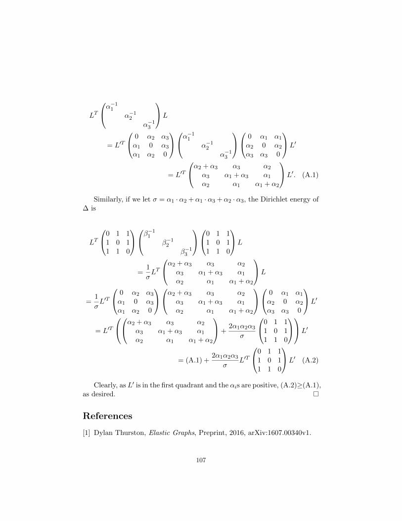
LT
α−1
1
α−12
α−13
L
= L′T
0 α2 α3
α1 0 α3
α1 α2 0
α−1
1
α−12
α−13
0 α1 α1
α2 0 α2
α3 α3 0
L′
= L′T
α2 + α3 α3 α2
α3 α1 + α3 α1
α2 α1 α1 + α2
L′. (A.1)
Similarly, if we let σ = α1 · α2 + α1 · α3 + α2 · α3, the Dirichlet energy of∆ is
LT
0 1 11 0 11 1 0
β−1
1
β−12
β−13
0 1 11 0 11 1 0
L
=1
σLT
α2 + α3 α3 α2
α3 α1 + α3 α1
α2 α1 α1 + α2
L
=1
σL′T
0 α2 α3
α1 0 α3
α1 α2 0
α2 + α3 α3 α2
α3 α1 + α3 α1
α2 α1 α1 + α2
0 α1 α1
α2 0 α2
α3 α3 0
L′
= L′T
α2 + α3 α3 α2
α3 α1 + α3 α1
α2 α1 α1 + α2
+
2α1α2α3
σ
0 1 11 0 11 1 0
L′
= (A.1) +2α1α2α3
σL′T
0 1 11 0 11 1 0
L′ (A.2)
Clearly, as L′ is in the first quadrant and the αis are positive, (A.2)≥(A.1),as desired.
References
[1] Dylan Thurston, Elastic Graphs, Preprint, 2016, arXiv:1607.00340v1.
107

[2] E.B. Curtis, D.Ingerman, and J.A. Morrow, Circular Planar Graphs andResistor Networks. Linear Algebra and its Applications 283 (1998) 115-150.
[3] R. L. Brooks, C. A. B. Smith, A. H. Stone, and W. T. Tutte, TheDissection of Rectangles into Squares. Duke Math. J. Volume 7, number1 (1940), 312-340.
[4] S. Alexander, V. Kapovitch, and A. Petrunin, Alexandrov meetsKirszbraun, Preprint, 2010, arXiv:1012.5636
108
Final ReportGTR+Γ+I Model Identifiability using a
Discrete Gamma Distribultion
Kees McGahanMentor: Elizabeth Houseworth
July 2016
Abstract
Phylogenetics is the study of trees that describe the evolution oforganisms. Mathematics provides models for DNA evolution thatenable Biologists to determine trees in a rigorous statistical frame-work. In order for these models to be useful, the models need to beidentifiable. That is, with an infinite amount of data from the truemodel, we should be able to recover all the parameters in that modeluniquely. One commonly used model, especially in phylogenetic soft-ware, is the GTR+Γ+I model, whose parameters include: T, the phy-logenetic tree, Q, the General Time Reversible (GTR) Markov ratematrix, and R, a random mutation rate taken from a mixture of aGamma distribution and invariant sites. This model has already beenshown to be identifiable when the Gamma distribution is continuous.However, all known software packages use a discrete version of theGamma distribution instead. In this REU project, we are exploringboth numerically and analytically whether the model with only tworate classes and no invariant sites is identifiable.1
1This material is based upon work supported by the National Science Foundation underGrant No. DMS-1461061.
109

This summer, I pursued a problem in mathematical biology, in the identi-fiability of trees. Phylogenetics is the study of trees that describe how speciesevolve. Biologists find themselves intrigued with the actual trees themselves,while the math involved revolves around the models used to generate saidtrees. Our work was centered around one such model, the GTR+Γ+I Modeland an attempt to prove the identifiability of this model for a specific case.
The main term to be aware of here is identifiabilty which means: if givenan infinite amount of data all of the model’s parameters can be uniquelydetermined. In our case the data comes in the form of DNA sequences ofour species. We shall assume two important details about our sequences:the first is that we have at least 4 species, as there is only one unrootedtree topology involving 3 species, and the second being that we assume oursequences contain an infinite amount of data. Through using these infinitesequences we hope to show that we can uniquely determine the parameters ofthe model. For the model we’re using, the GTR+Γ+I Model, the parametersare Q, T and R.
Our parameter Q will be some general time reversible rate matrix with atleast two non-zero distinct eigenvalues. The T that we are hoping to deter-mine is the phylogenetic tree itself, which we will consider to be unrooted andas having three or more distinct inter-species distances. The final parameterR, represents a rate of evolution. It has already been proved that if R is a acontinuous gamma distribution with mean 1 than the model will be identifi-able. My work this summer was with using R as a two rate class parameterstill with mean 1. We chose to work with a discrete Gamma distribution asthis typically is the distribution that software packages use, although theytypically use four rate classes. We hoped to be able to show that workingwith 2 rate classes would give some insight into using a discrete distribution,and possibly have our work extended to more rate classes.
Thus starting with 4 or more DNA sequences our hope is from pairwisesequence comparisons we can uniquely determine the above parameters. Dueto having an assumed infinite amount of data for pairwise comparisons wecan easily determine the stationary frequencies for each nucleotide and henceprobability matrix for any pair of species. We know through Markov chainsthat we can arrive at an equation that looks like
Pi,j(t) = Eeti,jQR
where we take the expected value of R, our discrete distribution of two rateclasses. It’s known that the eigenvectors of P are the eigenvectors of Q. Thus
110
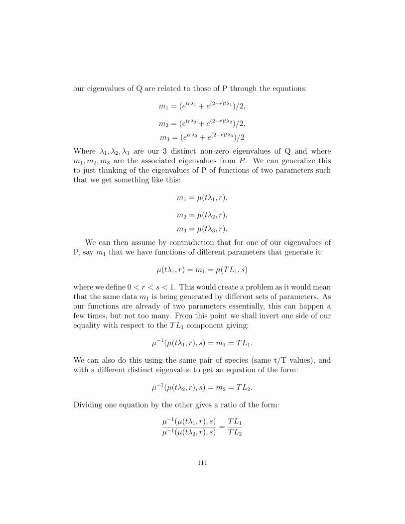
our eigenvalues of Q are related to those of P through the equations:
m1 = (etrλ1 + e(2−r)tλ1)/2,
m2 = (etrλ2 + e(2−r)tλ2)/2,
m3 = (etrλ3 + e(2−r)tλ3)/2
Where λ1, λ2, λ3 are our 3 distinct non-zero eigenvalues of Q and wherem1,m2,m3 are the associated eigenvalues from P . We can generalize thisto just thinking of the eigenvalues of P of functions of two parameters suchthat we get something like this:
m1 = µ(tλ1, r),
m2 = µ(tλ2, r),
m3 = µ(tλ3, r).
We can then assume by contradiction that for one of our eigenvalues ofP, say m1 that we have functions of different parameters that generate it:
µ(tλ1, r) = m1 = µ(TL1, s)
where we define 0 < r < s < 1. This would create a problem as it would meanthat the same data m1 is being generated by different sets of parameters. Asour functions are already of two parameters essentially, this can happen afew times, but not too many. From this point we shall invert one side of ourequality with respect to the TL1 component giving:
µ−1(µ(tλ1, r), s) = m1 = TL1.
We can also do this using the same pair of species (same t/T values), andwith a different distinct eigenvalue to get an equation of the form:
µ−1(µ(tλ2, r), s) = m2 = TL2.
Dividing one equation by the other gives a ratio of the form:
µ−1(µ(tλ1, r), s)
µ−1(µ(tλ2, r), s)=TL1
TL2
111

Which through some simplification of variables can be written as
C =µ−1(µ(λ1, r), s)
µ−1(µ(Bλ1, r), s)
where C is a constant and B is a constant with value greater than 1. Both Cand B are ratios of eigenvalues which is why we are allowed to assume thatB is greater than 1 as we can arbitrarily assume 1 eigenvalue greater thanthe other to get a value greater than 1. To make sure that this model isidentifiable we needed to show that for our ratio doesn’t equally C too manytimes.
Previous work, notably a proof of identifiability of the continuous caseshowed solved the similar problem through calculus and proving that the lineC was crossed only once or twice. We attempt a similar approach looking tofind a finite small amount of crossings of C. One way to do this is search forthe minima/maxima of the function as these will bound how many times ourratio can cross C. Thus we took the derivative of our ratio. One way to provethat our function only crosses C one time is if our derivative can be brokenup into two parts; one increasing and the other decreasing. We attemptedto do this and ended up with:
d
dx[µ−1(µ(x, r), s)
µ−1(µ(Bx, r), s)] =
µ−1(µ(Bx, r)s) 1µ′(µ−1(µ(x,r),s),s)
µ′(x, r) − µ−1(µ(x, r)s) 1µ′(µ−1(µ(Bx,r),s),s)
µ′(Bx, r)B
µ−1(µ(Bx, r), s)2.
Focusing only on the numerator we can get this too look like the followingby utilizing the fact that we have a difference in the numerator:
LHS =1
b[µ−1(µ(Bx, r)s)
µ−1(µ(x, r)s)][
µ′(x, r)
µ′(µ−1(µ(x, r), s), s)][µ′(µ−1(µ(Bx, r), s), s)
µ′(Bx, r)] − 1
and
RHS = (1
b−1)[
µ−1(µ(Bx, r)s)
µ−1(µ(x, r)s)][
µ′(x, r)
µ′(µ−1(µ(x, r), s), s)][µ′(µ−1(µ(Bx, r), s), s)
µ′(Bx, r)]+B−1.
These two functions yields a graph of the form:
112
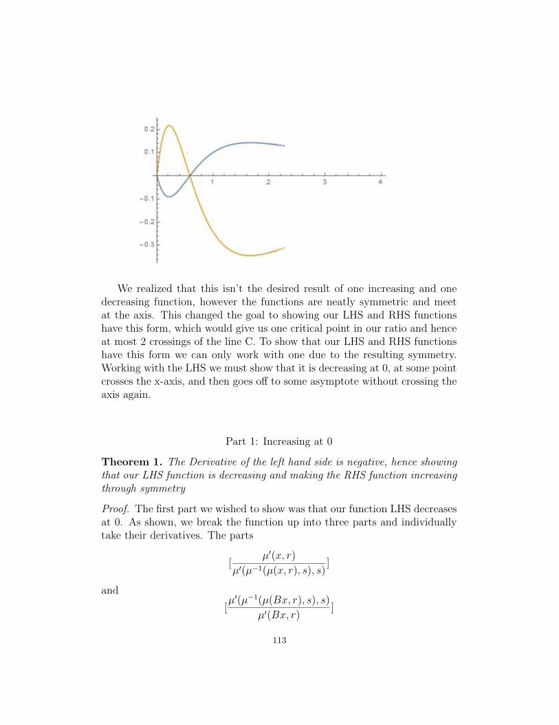
We realized that this isn’t the desired result of one increasing and onedecreasing function, however the functions are neatly symmetric and meetat the axis. This changed the goal to showing our LHS and RHS functionshave this form, which would give us one critical point in our ratio and henceat most 2 crossings of the line C. To show that our LHS and RHS functionshave this form we can only work with one due to the resulting symmetry.Working with the LHS we must show that it is decreasing at 0, at some pointcrosses the x-axis, and then goes off to some asymptote without crossing theaxis again.
Part 1: Increasing at 0
Theorem 1. The Derivative of the left hand side is negative, hence showingthat our LHS function is decreasing and making the RHS function increasingthrough symmetry
Proof. The first part we wished to show was that our function LHS decreasesat 0. As shown, we break the function up into three parts and individuallytake their derivatives. The parts
[µ′(x, r)
µ′(µ−1(µ(x, r), s), s)]
and
[µ′(µ−1(µ(Bx, r), s), s)
µ′(Bx, r)]
113
derive and evaluated at 0 pose no problems but when we take the derivativeof
[µ−1(µ(Bx, r)s)
µ−1(µ(x, r)s)]
and evaluate it at 0, we run into some 0/0 terms. As a work around weapproximate the µ−1 term with a second order Taylor series as shown in theaside.
ASIDE:
We know the second order Taylor series of µ(x, r) is
µ(x, r) = 1 + x+(r2) + (2 − r)2
4x2 + ...
To find the inverse of this expansion we shall first find the inverse of thefunction
(µ(x, r) − 1) = x+(r2) + (2 − r)2
4x2 + ...
Thus we know that (µ− 1)−1(x, s) has no constant term and thus has someexpansion that looks like
µ− 1)−1(x, s) = b1x+ b2x2 + ...
Since we know that
(µ−1)−1((µ(x, r)−1), s) = x = b1(x+(r2) + (2 − r)2
4x2+...)+b2(x+
(r2) + (2 − r)2
4x2+...)2+...
we can easily solve for the coefficients b1 and b2 which we can see are b1 = 1and
b2 = −(r2) + (2 − r)2
4This yields the second order Taylor series of
(µ− 1)−1(x, s) = x− (s2) + (2 − s)2
4x2 + ...
However this can also be used as the Taylor series for
µ−1(µ(x, r) − 1), s) = (µ− 1) − (s2) + (2 − s)2
4(µ− 1)2 + ...
114

because we just need to make sure that the Taylor series is still expandedabout 0. By evaluating our function at (µ(x, r)− 1) which at x = 0 is 0, ourµ−1 is being expanded about 0 as desired. Hence we can use this form, andthen substituting in for the above equations for µ yields
µ−1(µ(x, r)−1, s) = [x+(r2) + (2 − r)2
4x2+...]−(s2) + (2 − s)2
4[x+
(r2) + (2 − r)2
4x2 + ...]
2
Which simplifying to only the second order terms of our Taylor expansionabout zero gives
µ−1(µ− 1(x, r), s) = x+ [(r2) + (2 − r)2
4− (s2) + (2 − s)2
4]x2 + ...
BACK TO WORK
Now we can go back to looking at our function LHS and its derivative.We have:
LHS =1
b[µ−1(µ(Bx, r)s)
µ−1(µ(x, r)s)][
µ′(x, r)
µ′(µ−1(µ(x, r), s), s)][µ′(µ−1(µ(Bx, r), s), s)
µ′(Bx, r)] − 1
Looking at this in its three parts as
LHS =1
bXY Z − 1
where
X = [µ−1(µ(Bx, r)s)
µ−1(µ(x, r)s)]
Y = [µ′(x, r)
µ′(µ−1(µ(x, r), s), s)]
Z = [µ′(µ−1(µ(Bx, r), s), s)
µ′(Bx, r)]
115
we see that we’re solving for
LHS ′(0) = X ′Y Z +XY ′Z +XY Z ′.
Note that we’re excluding the 1/B term as it wont effect whether our funcitonis positive or negative when evaluated at 0. The derivatives of each of theparts are:
X ′ =Bµ′(Bx, r)µ−1(µ(x, r), s)µ′(µ−1(µ(x, r), s), s) − µ′(x, r)µ−1(µ(Bx, r), s)µ′(µ−1(µ(Bx, r), s), s)
[µ−1(µ(x, r), s)]2µ′(µ−1(µ(Bx, r), s), s)µ′(µ−1(µ(x, r), s), s)
Y ′ =µ′(µ−1(µ(x, r), s), s)µ′′(x, r) − µ′(x, r)µ′′(µ−1(µ(x, r), s), s) 1
µ′(µ−1(µ(x,r),s),s)µ′(x, r)
[µ′(µ−1(µ(x, r), s), s)]2
Z ′ =µ′(Bx, r)µ′′(µ−1(µ(Bx, r), s), s) 1
µ′(µ−1(µ(Bx,r),s),s)µ′(Bx, r) − µ′(µ−1(µ(Bx, r), s), s)µ′′(Bx, r)
[µ′(Bx, r)]2.
We also know what the components evaluated at 0 are:
µ(0, r) = (e0 + e0)/2 = 1
µ′(0, r) = (re0 + (2 − r)e0)/2 = 1
µ′′(0, r) = (r2e0 + (2 − r)2e0)/2 = (r2 + (2 − r)2)/2
Using the above information it is easy to see that both Y and Z evaluatedat 0 are both 1. Evaluating X at 0 would give 0/0 but using a first orderTaylor series we can see goes to B. So far that leaves us with LHS(0) =X ′+B ∗Y ′+B ∗Z ′. Then utilizing the information from the ASIDE for theµ−1(µ(x, r), s) terms that appear in X and evaluating at our derivatives weget something that simplifies out to
LHS ′(0) = B(1−B)(r2 + (2 − r)2 − s2 − (2 − s)2
4+r2 + (2 − r)2 − s2 − (2 − s)2
2).
All that’s left is to show that based on 0 < r < s < 1 and B > 1 this isnegative. The only part whose sign isn’t immediately determined is whether
r2 + (2 − r)2 − s2 − (2 − s)
is positive. We can see that this equals
(r + s)(r − s) + (s− r)(4 − r − s) =
116

(r − s)(r + s− 4 + r + s) =
2(r − s)[r + s− 2].
Which based on restrictions is positive. And therefore the equation
LHS ′(0) = 2Br2 + (2 − r)2 − s2 − (2 − s)2
4(1 −B)
is indeed negative due to the (1−B) term. Hence we’ve shown that derivativeof the LHS at 0 is negative, and so due to symmetry our LHS is decreasingand our RHS is increasing at x = 0.
Part 2: Goes to asymptote
I was unable to show that my functions LHS and RHS have asymptotesat some constant as X goes to infinity. However we were able to find theasymptote at infinity of the original ratio. Furthermore as this asymptote isa constant, we could hypothesize that the LHS and RHS would at infinity goto 0 as they are derivatives of our original ratio. Knowing this could providemore unique bounds for Part 3.
Lemma 1. The original ratio of [ µ−1(µ(x,r)s)µ−1(µ(Bx,r)s)
] goes to an asymptote of 1/Bat infinity.
Proof. Looking at the ratio we have
[µ−1(µ(x, r)s)
µ−1(µ(Bx, r)s)].
We know that
µ(x, r) =erx + e(2−r)x
2=e(2−r)x
2(1 + e−2(1−r)x).
This will be dominated by the e(2−r)x
2part as x goes to infinity. Thus as x
goes to infinity
µ−1(x, r) =ln (2x)
2 − r.
Therefore we can see that
µ−1(µ(x, r)s) =ln (2e(2−r)x)
2 − r=
2 − r
2 − sx.
117

Using the same logic we can see that
µ−1(µ(Bx, r)s) =ln (2e(2−r)Bx)
2 − r=
2 − r
2 − sBx.
Therefore as x goes to infinity our ratio
[µ−1(µ(x, r)s)
µ−1(µ(Bx, r)s)]
goes to 1/B.
Part 3: Crosses a small finite amount of times
We were unable to prove this but we do have a hypothesis that the LHS(and hence through symmetry RHS) both only cross the axis a finitely smallamount of times. In fact our hypothesis would by they cross only the axisonly once each. We believe it to be a true hypothesis due to extensive work inmathematica, and that we have yet to find a counterexample for any valuesof our parameters of r, s, B. A lot of our work in this area has been hoping tofind bounds that we could use to approximate our functions and work withthem instead. As of yet we haven’t managed to complete our goal.
118

References
Chai, Juanjuan, and Elizabeth A. Housworth. ”On Rogers’ proof of iden-tifiability for the GTR+ Γ+ I model.” Systematic biology (2011): syr023.
119