Embed Size (px)
Citation preview

University of North DakotaUND Scholarly Commons
Theses and Dissertations Theses, Dissertations, and Senior Projects
2013
Research about low permeability measurementJun HeUniversity of North Dakota
Follow this and additional works at: https://commons.und.edu/theses
Part of the Geology Commons
This Thesis is brought to you for free and open access by the Theses, Dissertations, and Senior Projects at UND Scholarly Commons. It has beenaccepted for inclusion in Theses and Dissertations by an authorized administrator of UND Scholarly Commons. For more information, please [email protected].
Recommended CitationHe, Jun, "Research about low permeability measurement" (2013). Theses and Dissertations. 130.https://commons.und.edu/theses/130

RESEARCH ABOUT LOW PERMEABILITY MEASUREMENT
by
Jun He
Bachelor of Science, Southwest Petroleum University, 1995
A Thesis Submitted to the Graduate Faculty
of the
University of North Dakota
In partial fulfillment of the requirements
for the degree of
Master of Science
Grand Forks, North Dakota August 2013

ii
Copyright 2013 Jun He

This thesis, submitted by Jun He in partial fulfillment of the requirements for the Degree of Master of Science from the University of North Dakota, has been read by the Faculty Advisory Committee under whom the work has been done and is hereby approved.
Date
Steve Benson
This thesis is being submitted by the appointed advisory committee as having met all of the requirements of the Graduate School of the University of North Dakota, and is
~ereby approved. s:. ~~ De~aduate School
Dat
iii

iv
Title Research about Low Permeability Measurement
Department Geology and Geological Engineering
Degree Master of Science
In presenting this thesis in partial fulfillment of the requirements for a graduate degree
from the University of North Dakota, I agree that the library of this University shall make
it freely available for inspection. I further agree that permission for extensive copying for
scholarly purposes may be granted by the professor who supervised my thesis work or, in
his absence, by the Chairperson of the department or the dean of the Graduate School. It
is understood that any copying or publication or other use of this thesis or part thereof for
financial gain shall not be allowed without my written permission. It is also understood
that due recognition shall be given to me and to the University of North Dakota in any
scholarly use which may be made of any material in my thesis.
Jun He
July 16, 2013

v
TABLE OF CONTENTS
TABLE OF CONTENTS .................................................................................................... v
LIST OF FIGURES .......................................................................................................... vii
LIST OF TABLES ............................................................................................................. ix
ACKNOWLEDGMENTS .................................................................................................. x
ABSTRACT ....................................................................................................................... xi
CHAPTER
I. INTRODUCTION .......................................................................................... 1
1.1. Previous Work ...................................................................................... 2
1.1.1. The Pulse-decay Method ....................................................... 3
1.1.2. The Oscillating Pulse Method ............................................... 7
1.1.3. Gas Research Institute (GRI) Method ................................... 8
1.2. Purpose/Thesis Statement .................................................................... 9
II. METHOD ..................................................................................................... 11
2.1. Sampler and Equipment ...................................................................... 11
2.2. Derivation of Diffusivity Equation .................................................... 14
2.3. Method 1: Downstream Pressure Build-up Measurement Method.... 20
2.3.1. Formula Derivation ............................................................ 21

vi
2.3.2. Measurement Procedure ..................................................... 25
2.4. Method 2: Radius-of-Investigation Measurement Method ................ 26
2.4.1. Formula Derivation ............................................................ 28
2.4.2. Measurement Procedure ..................................................... 30
III. RESULTS & DISCUSSION ...................................................................... 33
IV. CONCLUSIONS ........................................................................................ 41
REFERENCES ................................................................................................................. 43
NOMENCLATURE .......................................................................................................... 47

vii
LIST OF FIGURES
Figure Page
1-1 Schematic diagram for pulse decay permeability system ........................................ 4
1-2 Changes of the pressure during a sinusoidal oscillation pulse method ................... 8
1-3 Schematic diagram for GRI permeability system.................................................... 9
2-1 Core plug sampling system used in this study ........................................................ 11
2-2 Experimental setup for permeability measurement under stresses ........................ 12
2-3 Images of core and core holder for low permeability test system ......................... 13
2-4 Images of the end caps........................................................................................... 13
2-5 Schematic diagram of AutoLab-1500 low permeability system ........................... 14
2-6 Gas flows through core .......................................................................................... 15
2-7 Changes of the pressures from a downstream pressure build-up method ............. 21
2-8 ln(∆p) vs. time plot for core sample 1 ................................................................... 24
2-9 End times of downstream pressure build-up method and radius of investigation
method................................................................................................................... 31
3-1 Changes of the pressure during one experiment .................................................... 33
3-2 ln(∆p) vs. time plot for core sample 2 ................................................................... 34
3-3 ln(∆p) vs. time plot for core sample 3 ................................................................... 35
3-4 ln(∆p) vs. time plot for core sample 4 ................................................................... 35

viii
3-5 ln(∆p) vs. time plot for core sample 5 ................................................................... 36
3-6 ln(∆p) vs. time plot for core sample 6 ................................................................... 36
3-7 Comparison of permeabilities measured by three methods ................................... 39

ix
LIST OF TABLES
Table page
3-1 Permeability measured by oscillating pulse method ............................................. 37
3-2 Permeability measured by downstream pressure build-up method ....................... 37
3-3 Permeability measured by radius-of-investigation method ................................... 38

x
ACKNOWLEDGMENTS
I would like to thank my committee members, Drs. Kegang Ling (chairman), Richard
LeFever, and Steve Benson, for their advice during the research and their critical reviews
of the thesis. I would like to especially thank Dr. Kegang Ling for his suggestions on
the problem, for his constant encouragement, and for his support throughout my study.
Thanks are also extended to the University of North Dakota, the Harold Hamm School of
Geology and Geological Engineering, and Petroleum Engineering Department for
providing me an excellent education as well as facilities and patience, while I completed
my research about low permeability measurement. This research is supported in part by
the U.S. Department of Energy (DOE) under award number DE-FC26-08NT0005643. I
would also like to thank the Wilson M. Laird Core and Sample Library and the North
Dakota Geological Survey for providing core samples for this study.

xi
ABSTRACT
Petroleum exploration and production from shale formations have gained great attention
throughout the world in the last decade. Producing the hydrocarbons from shale is
challenging because of the low porosity and permeability. It is imperative to investigate
permeability of the shale formations in order to better understand the performance of
wells that are producing hydrocarbons from shale. Permeability is also one of key
parameters in modeling fluids flow in matrix in reservoir simulation. Due to the low or
very low permeability, the measurement of permeability is time consuming and expensive.
These factors often limited the ability to perform permeability measurement on large
numbers of samples. Thus, there is a great demand for a method that can significantly
reduce the time of the measurement, which leads to lower cost in core analysis.
In this study a downstream pressure build-up method, which is more operational, as
in this method the ratio of volume of the upstream reservoir, V1, to volume of the
downstream reservoir, V2, approaches infinite.
In addition, we developed another new method to determine the permeability of low
to very low permeability rock based on Darcy’s law and the radius-of-investigation
concept, which has been used in the well test design and analysis. Our method evaluates
the permeability under unsteady-state flow, which requires a shorter time to determine

xii
flow capacity of low permeability rock. The new approach is different from the existing
methods, such as GRI, oscillating pulse, and pulse decay methods. The significance of
this investigation is that it overcomes the limitations in existing methods thus becomes an
important supplement to the existing methods.

1
CHAPTER I
INTRODUCTION
Permeability is a property of a porous medium and is an indicator of its ability to
allow fluids flow through its inter-connected pores. Permeability is an inherent
characteristic of the porous media only. It depends on the effective porosity of the porous
media (Triad, 2004).
The fundamental SI unit of permeability is m2, but the Darcy (D), named after
French engineer Henry Darcy, is a practical unit for permeability. One Darcy is defined as
follows: a permeability of one Darcy will allow a flow of 1 cm3/s of fluid of 1 centipoise
(cp) viscosity through an area of 1 cm2 under a pressure gradient of 1 atm/cm. One Darcy
equals 0.986923 × 10 -12
m2. In the oil and gas industry, a smaller unit of permeability,
milli-darcy (mD), is used more commonly because the permeability for most rocks is less
than one Darcy, and for the low permeability rocks, the use of micro-Darcy (μD) or
nano-Darcy(nD) is common.
The range of the permeability of the petroleum reservoir rocks may be from 0.1 to
1,000 mD. A rock is considered to be tight when its permeability is below 1 mD (Triad,
2004). However, this criterion has been lowered to values of 0.1mD (Law & Spencer,
1993) due to the application of the new stimulation techniques to increase oil and gas

2
production. Tight rocks have been extensively studied for a wide range of applications
that include CO2 geological storage, deep geological disposal of high-level, long-lived
nuclear wastes, and production of oil and gas from unconventional reservoirs. In the
recent years, the increasing demands for oil and gas have stimulated the explorations and
productions of petroleum from low permeability formations, such as shale and limestone.
Producing the hydrocarbons from those formations is challenging because of their low
porosity and permeability. More realistic fluid flow simulation to model the process of
producing the hydrocarbons in those formations requires more accurate measurements of
permeability. Also it is urgent to investigate permeability of those low permeability
formations in order to gain better understanding of the process of well producing
hydrocarbons from shale.
Based on experimental work from Darcy, many permeability measurement methods
have been presented in order to improve the measurement accuracy, and precision, and to
reduce the measurement time. Some methods are used in laboratory, some are in field,
and some can be used in both. In this study, we focused on the methods that can be used
in the laboratory.
1.1. Previous Work
Conventional methods of measuring permeability in the laboratory utilize
steady-state flow. Steady-state flow, or a constant pressure gradient flow, is established

3
through the core plug, and the permeability is calculated from the rate of the measured
flow and the pressure gradient. But this method is not adequate when measuring
permeability in the low permeability samples. Not only the low flow rates across the
core plug are difficult to be measured and controlled, but the tests are also quite time
consuming.
Because of the disadvantage of the steady-state flow, unsteady state flow, a condition
under which the pressure gradient is a function of time, was studied. With the
measurements of the volumetric flow rate, upstream, and downstream pressures, the
permeability can be calculated. Since Brace et al. (1968) introduced a transient flow
method to measure permeability of Westerly Granite, many methods that based on
unsteady state flow theory have been proposed to measure the permeability of tight rocks.
Although many unsteady state methods have been developed to measure
permeability, most of them can be categorized into three types, which are pulse decay
method, oscillating pulse method, and Gas Research Institute (GRI) method (Tinni et al.,
2012).
1.1.1. The Pulse-decay Method
The pulse decay method is a transient method. The experimental arrangement is
shown schematically in Figure 1-1. The sample has both upstream reservoir and
downstream reservoir with the initial condition of uniform pore, upstream and

4
downstream pressures. When a pressure pulse is applied at the upstream end of a core
plug and propagates through core to the downstream reservoir, the pressure pulse will
decay over time. The decay characteristics depend on the permeability, size of the
sample, volumes of upstream and downstream reservoirs, and physical characteristics of
the fluid. Permeability is estimated by analyzing the decay characteristics of the pressure
pulse.
Figure 1-1 Schematic diagram for pulse decay permeability system
Brace et al. (1968) suggested a transient flow, or pressure-pulse, technique to
determine the permeability of granite. In their experiment the decay of pressure was
measured and the permeability was estimated through the following equation.
t
2
1
2f1 eV
V
Vp)pp(
......................................................................................... (1-1)
Where
)V
1
V
1(
cL
kA
21
............................................................................................(1-2)
A is cross-sectional area, L is length of sample, μ is fluid viscosity, c is fluid
compressibility, V1 and V2 are volumes of upstream and downstream reservoirs, p1 and p2
Upstream reservoir Downstream reservoir
VALVE
p1 V1 p2 V2 Core Vp
Hydrostatic Pressure
Core Holder

5
are pressures of upstream and downstream reservoirs, pf is final pressure, and Δp is the
pressure difference between the upstream reservoir and the downstream reservoir at time
= 0.
Permeability is calculated from Equation (1-2) after obtaining α from Equation (1-1),
which is calculated as a function of pressure decay (P1-Pf) on a semi-logarithm scale
against time. It should be noted that Δp must be small for this equation to be valid.
Dicker and Smits (1988) improved the pressure pulse-decay method by showing a
general solution of the differential equation which describes the decay curve. Based on
the solution, they pointed out that fast and accurate measurements are possible when the
volumes of the upstream and downstream reservoirs in the equipment are equal to the
pore volume of the sample. Jones (1997) developed a technique to reduce measurement
time in pulse-decay experiment. In his approach, permeability is calculated from
“late-time”measurements. Jones emphasized that the volumes of the upstream and
downstream reservoirs should be equal and pointed out that the initial pressure
equilibration step is the most time-consuming part of the pulse-decay technique. To
avoid the equilibrium state, Johns’ method utilizes a smooth pressure gradient, which
requires smaller upstream and downstream reservoirs. Metwally (2011) gave another
pulse-decay method by keeping the upstream pressure constant, which leads to an
infinitely large volume of the upstream reservoir so that the ratio of upstream volume
over downstream volume is infinite. Thus, the solution of the pulse-decay

6
measurements can be simplified and the decay time can be reduced.
The followings are other important studies on the pulse-decay method: Hsieh et al.
(1981) applied transient pulse test to measure the hydraulic properties of the rock samples
with low permeability. Le Guen et al. (1993) employed pulse-decay method to measure
permeability of rocksalt under thermo-mechanical stress. Luffel et al. (1993) reviewed
three methods to measure shale permeability. Hildenbrand et al. (2002 and 2004)
studied the gas effective permeability of fine-grained sedimentary rock using downstream
pressure-time relationship under Darcy flow condition. Homand et al. (2004) applied
the modified pulse test proposed by Hsieh (1981) to characterize permeability of low
permeable rocks. Billiotte et al. (2008) used transient pulse technique to measure the
permeability of mudstones. They observed that the gas permeability is decreasing with
the increase of the confining stresses due to the closing of some micro fissures in the
sample. This reduction is irreversible after a loading-unloading cycle. Cui et al. (2009)
presented models to correct adsorption terms during pulse-decay measurements on
crushed samples and in the field experiments. Cui et al. (2009) also used model to
determine the permeability or diffusivity from on-site drill-core desorption test data.
Metwally and Sondergeld (2011) built a new apparatus to simulate the permeability of
tight rock samples over a range of the effective pressures based on the pulse decay
technique.

7
1.1.2. The Oscillating Pulse Method
In 1990, Kranz et al. presented an oscillating pulse method to determine the
permeability and diffusivity of the rock samples. They provided one optimized
measuring system and the oscillation frequency for each of the rock types. Fischer and
Paterson (1992) measured permeability and storage capacity in three types of rocks
(marble, limestone, and sandstone) during deformation at high pressure and temperature.
The oscillating pulse method estimates rock permeability by interpreting the
amplitude attenuation and the phase retardation in the sinusoidal oscillation of the pore
pressure as it propagates through a sample.
At the beginning of the experiment, the sample pore pressure, the upstream pressure,
and the downstream pressure are stabilized. Then a sinusoidal pressure wave is
generated in the upstream and propagates through a core plug. Using the information of
the amplitude attenuation and phase shift between the upstream pressure wave and the
derived downstream pressure wave at the downstream side of the sample, the
permeability can be obtained (see Figure 1-2).
This method can measure the permeability of tight rock in a relative short time
without destroying rock sample. The accuracy of permeability obtained from this
method relies on the signal-to-noise ratio and data analysis techniques. The optimum
frequency of the oscillation and the ratio of the downstream to upstream pore pressures
depend upon the sample size and the magnitude of permeability (Kranz et al., 1990).

8
Therefore, the calculated permeability contains large uncertainty when measured under
the condition of low signal-to-noise ratio. Moreover, different analysis techniques can
result in different permeabilities in the same experiment.
Figure 1-2 Changes of the pressure during a sinusoidal oscillation pulse method
1.1.3. Gas Research Institute (GRI) Method
GRI method (Luffel, Hopkins, & SchettlerJr., 1993) differs from the previous
methods by carrying out the measurement on crushed rock sample. The experimental
arrangement is shown in Figure 1-3. The crushed rock particles are in Chamber 2.
Initially the pressure in Chamber 1 is greater than the pressure in Chamber 2. Then
open Gas Outlet Valve to allow gas flow from Chamber 1 to Chamber 2. The pressure

9
decay in the rock particles can be observed. Permeability is obtained through the
analysis of this pressure decay over time. 992)
Figure 1-3 Schematic diagram for GRI permeability system
GRI method requires shorter experimental time when compared with other methods.
However the permeability measured from the crushed samples can differ by two to three
orders of magnitude from the companion intact samples (Passey et al., 2010 and Tinni et
al., 2012). Also microcracks in the crushed particle violate the assumption in the GRI
method, which leads to an overestimate of permeability (Tinni et al., 2012).
1.2. Purpose/Thesis Statement
Due to the properties of the low or very low permeability, the measurement of the
tight-rock permeability is time consuming and expensive. An inexpensive method that
tremendously reduces the measurement time in core analysis is needed.
Gas Tank
Gas Outlet Valve
(to Chamber 2) Gas Inlet Valve
Pressure Gauge 1
Chamber 2 Chamber 1
Pressure Gauge 3 Pressure Gauge 2
Gas
Vent Valve

10
After reviewing the previous work, we chose pulse decay method as our base method
to measure permeability in the tight rock. Because the pulse decay method does not
destroy the core plug as GRI method and has higher confident level than oscillating pulse
method.
We found that to improve the pulse decay method, alterations in the volumes of the
sample pore space, the upstream reservoir, and the downstream reservoir are necessary.
Theoretically, the perfect result can be obtained only when those volumes are equal,
V1=V2=Vp (Dicker and Smits, 1988: and Jones, 1997), but it is not easy to obtain because
the pore space of a core plug (2×1 inch) is very small. A long time for pre-balance is
needed even if only the equal volumes between V1 and V2 are required.
In our study, we first investigated the downstream pressure build-up method, which
belongs to pulse decay method, but it is more operational since it does not require the
equal volumes between V1 and V2. We also developed another method, which is called
radius-of-investigation method, to determine the permeability of low to very low
permeability rock, by utilizing Darcy law and the radius-of-investigation concept. This
radius-of-investigation method is very useful in decreasing the time required for a test.

11
CHAPTER II
METHOD
2.1. Sampler and Equipment
Middle Bakken core samples, supplied by the North Dakota Geological Survey's
Wilson M. Laird Core and Sample Library, were chosen as the specimens to represent the
tight rocks.
Due to the fragile nature of the core, before preparing the core plugs, we pre-cooled
the core at -85 0C for 20 days and drilled with liquid N2 coolant (Figure 2-1). The core
plugs are cylindrical with dimension of one inch in diameter and two inches long.
Figure 2-1 Core plug sampling system used in this study

12
The equipment that is used to perform our experiments is AutoLab-1500, which is
made by New England Research Inc. Figure 2-2 presents a conceptual diagram of the
gas flow in AutoLab-1500. The cylindrical core plug was covered with copper sheet
(Figure 2-3) in order to make a gas-tight seal on the cylindrical wall of the sample, and
for applying radial confining pressure. Then the core plug was mounted in a sample
holder with flexible rubber sleeves at both ends of the plug (Figure 2-3). At last, the
sample holder was put into a vessel flooded with mineral oil, in which the sample can be
hydrostatically compressed by applying force to plug by hydraulic means.
Mineral
Oil
Fluid
Pump
Electrical
Heater
Rock
Core
TT1
Strain Gage 1
PT3
Nit
rog
en
Computer
Data Logger
Strain Gage 2
Axial Stress
Confining
Pressure
Fluid
Pump
Deplete
Valve
PT1
PT2
PT4
Figure 2-2 Experimental setup for permeability measurement under stresses

13
Figure 2-3 Images of core and core holder for low permeability test system
Figure 2-4 Images of the end caps (left: downstream cap, right: upstream cap)
Figure 2-4 shows that the two end caps contain two axial ports for transporting gas to
and from the sample and each of them has radial and circular grooves for distributing gas
to its entire surface. The upstream end-cap connects to a servo-controlled hydraulic
intensifier, which is used to control and monitor the upstream pressure (p1). The
downstream pressure at the other end of the sample is monitored by a miniature pressure
transducer, which is located in the downstream end-cap. To minimize the volume of the
downstream reservoir, a small pocket is implemented inside the downstream end-cap
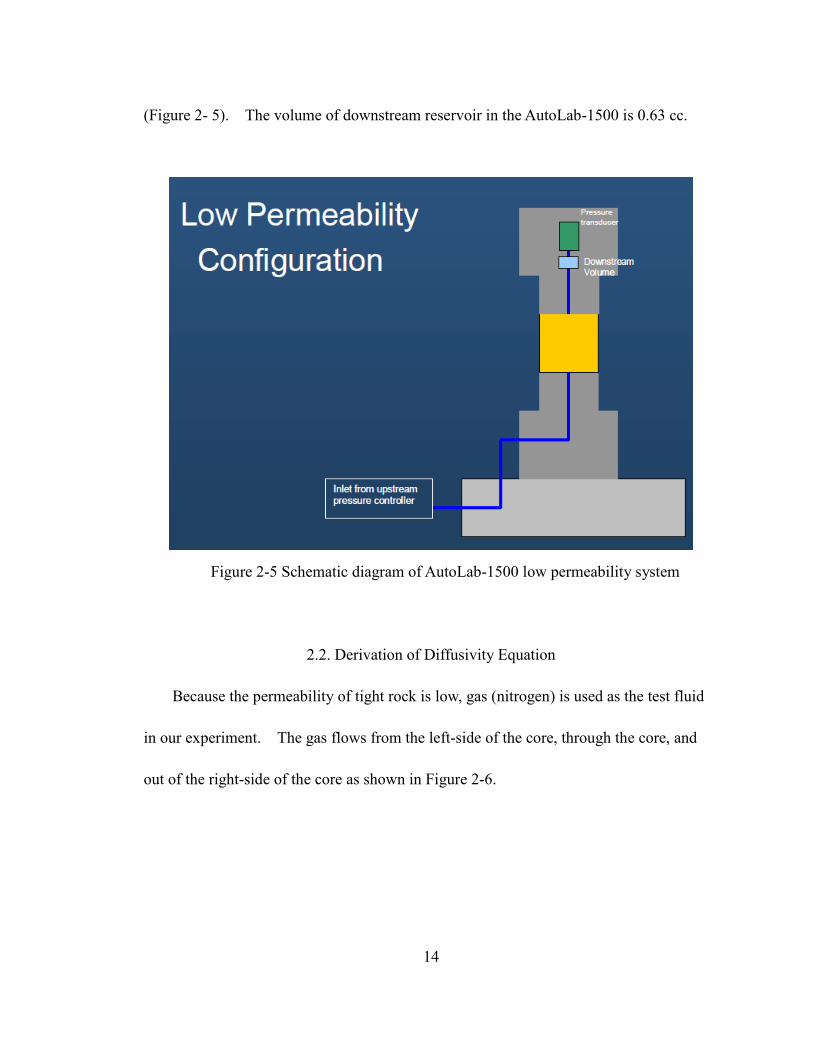
14
(Figure 2- 5). The volume of downstream reservoir in the AutoLab-1500 is 0.63 cc.
Figure 2-5 Schematic diagram of AutoLab-1500 low permeability system
2.2. Derivation of Diffusivity Equation
Because the permeability of tight rock is low, gas (nitrogen) is used as the test fluid
in our experiment. The gas flows from the left-side of the core, through the core, and
out of the right-side of the core as shown in Figure 2-6.

15
Figure 2-6 Gas flows through core
To derive the diffusivity equation of the gas flow in the core, following assumptions
are made: 1) the core is homogeneous, 2) the properties of the rock are constant, 3) the
flow in the cylindrical core is laminar, and 4) the flow in the core is isothermal.
Considering a control volume (from x to x+Δx), which is the volume that the gas flows in
from x and out at x+Δx during a certain time period Δt, the law of the mass conservation
provides:
MassdAccumulate Mass- Mass outin ..........................................................................(2-1)
The mass of gas that flows into the section is:
tAvρMass xxin .........................................................................................................(2-2)
where Δt is the time period, ρx is the gas density at location of x during Δt, vx is the gas
velocity at x in the x direction during Δt, and A is the cross-sectional area of the core
plug.
The mass of gas that flows out of the section is:
tAΔvρMass ΔxxΔxxout ...............................................................................................(2-3)
Core
△p
x+△x
p+△p
x △x
p
K D
P2
x=L x=0
P1
Control
Volume
qg
A
L

16
where Δt is the time period, ρx+Δx is the gas density at location of x+Δx during Δt, vx+Δx is
the gas velocity at x+Δx position during Δt, and A is the area of the cross section of the
core plug.
The mass of gas that accumulates inside the section is:
xAΔφρxAΔφρ MassdAccumulate ttΔttΔtt ...........................................................(2-4)
Where ρt+Δt is the gas density in the control volume at t+Δt, φt+Δt is the rock porosity of
the control volume at t+Δt, ρt is the gas density in the control volume at t, φt is the rock
porosity of the control volume at t, Δx is the incremental distance in x direction, and A is
the area of cross section of the core plug.
Substituting Equations (2-2), (2-3), and (2-4) into Equation (2-1), we have
xAΔφρxAΔφρtAΔvρtAΔvρ ttΔttΔttΔxxΔxxxx
Dividing both sides with AΔxΔt and taking the limits as Δx and Δt go towards zero, the
resulting equation becomes a linear diffusivity equation, which is
Δt
φρφρlim
Δx
vρvρlim ttΔttΔtt
0Δt
xxΔxxΔxx
0Δx
)ρφ(t
ρvx
.......................................................................................................(2-5)
Using Darcy’s law, we can express gas velocity as
x
p
μ
kv
..................................................................................................................(2-6)
where k is permeability, μ is gas viscosity, x
p
is the pressure drop along x direction.
According to the real gas law, we can calculate gas density using

17
z
p
RT
Mρ
......................................................................................................................(2-7)
where M is molar mass, R is the ideal gas constant, T is the temperature of the gas, p is
the pressure of the gas, and z is gas z-factor.
Substituting Equations (2-6) and (2-7) into Equation (2-5), we get
φ)z
p
RT
M(
t)
x
p
μ
k(
z
p
RT
M
x
Based on our assumptions above, temperature (T) and permeability (k) are constants, we
divide both sides byRT
Mto get
φ)z
p(
tx
p
μz
pk
x
which can be simplified as
φ)z
p(
tx
p
μz
p
xk
..........................................................................................(2-8)
Using gas pseudo-pressure concept (Al-Hussainy, 1966), the gas pseudo-pressure is
defined as
dpμz
p2)pm(
p
pb
..............................................................................................................(2-9)
where p is the pressure and pb is the low base pressure.
Assuming isothermal and small pressure drop, we take the derivatives with respect to
x, and t at both sides of the Equation (2-9). The equation becomes
)pdμz
p2(
x)]p[m(
x
p
pb

18
which can be simplified as
x
p
μz
p2)]p[m(
x
....................................................................................................(2-10)
and
)pdμz
p2(
t)]p[m(
t
p
pb
which can be simplified as
t
p
μz
p2)]p[m(
t
..................................................................................................... (2-11)
If we use m(p) to rearrange Equation (2-8), it becomes
φ)μz
p2(
tμ
x
p
μz
p2
xk
which can be written as
t
φ
μz
p2μ)
μz
p2(
tμφ)pm(
xk
2
2
....................................................................(2-12)
Assuming μ is constant, Equation (2-12) can be rearranged to
t
φ
z
p2)
z
p(
tz
φ2)pm(
xk
2
2
........................................................................(2-13)
If the right-hand side (RHS) of the Equation (2-13) can be transformed into a new
form so that the only variable required to be differentiated is m(p), then solving the
equation will be much easier.
Based on this hypothesis, the first item of the RHS of the Equation (2-13),
)z
p(
tz
φ2
needs to be modified. Recalling real gas law, we have

19
znRTpV
nRTV
1
z
p
Inserting nRTV
1
z
p into )
z
p(
t
, we get
t
p
p
v
V
1nRT
t
p)
V
1(
pnRT)
V
1(
tnRT)
z
p(
t 2
...................................(2-14)
The coefficient of isothermal compressibility of gas is )p
V(
V
1cg
. Substituting cg
into Equation (2-14), we get
t
pc
z
p
t
pc
v
nRT)
z
p(
tgg
................................................................................(2-15)
The second term of the RHS of the Equation (2-13) is t
φ
z
p2
. According to the
rock pore compressibility, )p
(1
cs
, we have
t
pc
t
p
p
φ
t
φs
...............................................................................................(2-16)
Finally, substituting Equation (2-15), and (2-16) into (2-13) gives
t
pc
z
p2
t
pc
z
p
z
φ2)pm(
xk sg2
2
which can be simplified as
t
p
z
p2)cc()pm(
xk sg2
2
Substituting Equation (2-11) into the above equation gives
)pm(t
c)pm(x
k t2
2
which can be written as

20
)pm(tk
c)pm(
x
t
2
2
........................................................................................(2-17)
where ct is the total compressibility ( sgt ccc ).
Now the diffusivity Equation (2-5) for linear gas flow becomes Equation (2-17).
When pressure difference between the two sides of the core is small, the coefficient in the
RHS of the Equation (2-17) can be considered as constant. Based on this assumption,
Equation (2-17) can be treated as a linear partial differential equation.
2.3. Method 1: Downstream Pressure Build-up Measurement Method
In our downstream pressure build-up method, a constant pressure is applied at the
upstream end of the core plug throughout the entire test and the pressure build-up is
observed in the downstream reservoir when the gas flows into it. Figure 2-7 shows an
example of the pressure change in the downstream reservoir as a function of time.
21
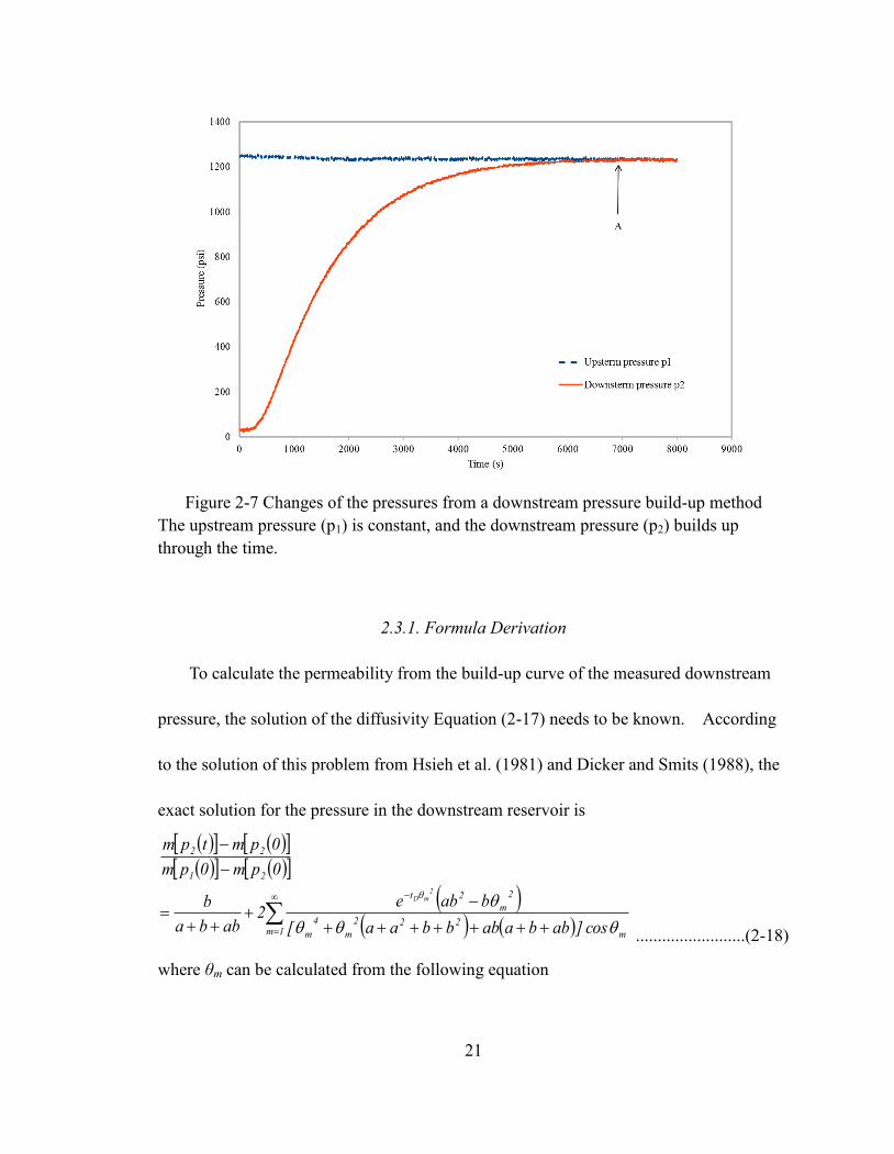
Figure 2-7 Changes of the pressures from a downstream pressure build-up method
The upstream pressure (p1) is constant, and the downstream pressure (p2) builds up
through the time.
2.3.1. Formula Derivation
To calculate the permeability from the build-up curve of the measured downstream
pressure, the solution of the diffusivity Equation (2-17) needs to be known. According
to the solution of this problem from Hsieh et al. (1981) and Dicker and Smits (1988), the
exact solution for the pressure in the downstream reservoir is
1m m
222
m
4
m
2
m
2t
21
22
cos]abbaabbbaa[
babe2
abba
b
0pm0pm
0pmtpm
2mD
.........................(2-18)
where θm can be calculated from the following equation

22
ab
)ba(tan
2
............................................................................................................(2-19)
where a is the ratio of the sample pore volume (Vp) over the upstream reservoir volume
(V1), and b is the ratio of the sample pore volume over the downstream reservoir volume
(V2), )V
Vb,
V
Va(
2
p
1
p .
In the Equation (2-18) the dimensionless time, tD, is defined as:
2
t
DLc
ktt
.................................................................................................................(2-20)
By careful observation we find that uz can be treated as constant at low pressure
range, which is the pressure conditions used in this study. According to Equation (2-9),
which is
pdμz
p2)pm(
p
pb
, the left-hand side (LHS) of Equation (2-18) can be written as
)0(p)0(p
)0(p(t)p
dpuz
p2dp
uz
p2
dpuz
p2dp
uz
p2
0pm0pm
0pmtpm2
2
2
1
2
2
2
2
)0(p
)0(p
)0(p
)0(p
(t)p
)0(p
)0(p
)0(p
21
22
1
2
2
2
2
2
2
2
....................................(2-21)
Next, we simplify the RHS of Equation (2-18). The upstream pressure p1 is
invariant throughout the test, which implies that the upstream volume V1 leads to infinity,
so the ratio of the sample pore volume to the upstream volume (1
p
V
Va ) can be
considered as zero. Substituting a as zero and the Equation (2-21) into Equation (2-18),
we obtain:
1m m
22
m
4
m
2
m
t
2
2
2
1
2
2
2
2
cos)]bb([
)b(e21
)0(p)0(p
)0(p)t(p2
mD

23
which can be written as
1m m
22
m
4
m
2
mt
2
2
2
1
2
2
2
1
cos)]bb([
be2
)0(p)0(p
)t(p)0(p 2mD
.......................................(2-22)
For a = 0, Equation (2-19) becomes
btan
......................................................................................................................(2-23)
which can be written in the following format
b
cos
sin that leads to
22
2
bcos
.
This equation contains an infinite numbers of solution θm and the values of the solutions
increase monotonically. Thus 22
m
m1m
m
b)1(cos
. Inserting it into Equation
(2-22), we obtain
1m22
m
4
m
22
m
4
m
1m
t
2
2
2
1
2
2
2
1
)bb(
bb)1(e2
)0(p)0(p
)t(p)0(p 2mD
..............................................(2-24)
Dicker and Smits (1988) mentioned that Equation (2-24) is not fully single
exponentially decreasing because the volume of upstream reservoir is much larger than
the volume of downstream reservoir. But they indicated that the experiment under this
condition is rapid. In addition, a single exponential equation fit very well with the
downstream pressure build-up curve which was built later if a right interval was selected.
Thus, we simplified Equation (2-24) to:
)bb(
bb2e
)0(p)0(p
)t(p)0(p22
1
4
1
22
1
4
1t
2
2
2
1
2
2
2
12
1D

24
Let )t(p)0(p)t(p2
2
2
1 , we get
21Dt
22
1
4
1
22
1
4
1e
)bb(
bb2
)0(p
)t(p
which can be written as
21Dt
22
1
4
1
22
1
4
1e
)bb(
bb)0(p2)t(p
..................................................................(2-25)
Taking the natural log of Equation (2-25) yields
2
1D22
1
4
1
22
1
4
1t
)bb(
bb)0(p2ln)t(pln
....................................................(2-26)
Substituting tD from Equation (2-20) into Equation (2-26), we get
tLc
k
)bb(
bb)0(p2ln)t(pln
2
t
2
1
22
1
4
1
22
1
4
1
...................................................(2-27)
Figure 2-8 ln(∆p) vs. time plot for core sample 1

25
Assigning2
t
2
1
Lc
ks
, which is the slope of the pressure difference in a logarithm as
a function of time based on Equation (2-27) (Figure 2-7); permeability can be easily
obtained from Equation (2-28) when s is fitted in Figure 2-8.
sLc
k2
1
2
t
...........................................................................................................(2-28)
Using the Taylor series of tanθ , 3tan
3
, we can calculated θ1 from Equation
(2-23): 1
3
11
b
3
, and
)b3
411(
2
32
1 ..............................................................................................(2-29)
Substituting Equation (2-29) into Equation (2-28), we obtained:
b3
4133
sLc2k
2
t
. ......................................................................................................(2-30)
Considering that22
p
V
AL
V
Vb
, the equation becomes
2
2
t
V3
AL4133
sLc2k
...................................................................................................(2-31)
2.3.2. Measurement Procedure
The determination of the permeability is a three-step process, namely installing the
core plug into AutoLab-1500, running the test, and analyzing the resultant data.

26
1) Installing the core plug into AutoLab-1500
First, the core holder is placed into the vessel, then the vessel is filled with mineral
oil and the confining pressure is increased to the desired level (pc). The valve between
the core plug and the upstream reservoir is closed. Dry nitrogen is used to fill the
upstream reservoir and the upstream pressure is increased to the desired level (p1). The
downstream pressure is atmospheric pressure. Notice that the confining pressure must
be greater than the upstream pressure.
2) Running the test
The starting time is recorded when the valve between the core plug and the upstream
reservoir is opened. During the whole test, the upstream and the confining pressures are
constant. The pressures are monitored and recorded at both the upstream and
downstream ends of the sample. The test is end when the downstream pressure is equal
to the upstream pressure, which is at the point ‘A’ in the Figure 2-7.
3) Analyzing the resultant data
First the pressure difference is calculated in a logarithm scale from equation:
)t(p)0(pln)t(pln2
2
2
1 . Then form the plot by function fitting (Figure 2-8), we get
the slope, s. Finally, using Equation (2-31), we can obtain the permeability of the rock.
2.4. Method 2: Radius-of-Investigation Measurement Method
Based on the radius-of-investigation concept (Lee, 1982), we proposed a new

27
laboratory core permeability measurement method.
When doing the permeability test using the downstream pressure build-up method,
we observed that the downstream pressure did not increase immediately when the
upstream reservoir connected with the core plug. The lower the permeability is, the
longer delay time is observed.
Based on this phenomenon, a correlation can be found between the permeability and
the delaying time. Through this correlation, the permeability can be measured in a
much shorter time (Figure 2-8) when compared with the previous method.
In our research, we discovered that the radius-of-investigation concept (Lee, 1982)
could be useful for uncovering the relationship between the permeability of rock and the
waiting time before the downstream pressure increases. Radius of investigation is the
distance that a pressure disturbance moves into a formation when it is caused from the
well. Lee pointed out that it is possible to calculate the maximum distance that a pressure
disturbance can reach at any time, if we know the properties of rock and fluid, such as the
rock permeability and porosity, fluid viscosity, and the compression of both rock and
fluid. This means that the maximum distance of pressure disturbance is a function of
permeability and time, when other parameters are constants.
Thus, the time that a pressure disturbance spends in a rock is a function of the
permeability of the rock, if we know the length of the rock. Our hypothesis is that we
can calculate the low permeability in laboratory by measuring the delaying time, which is

28
the time that the pressure disturbance propagates from the upstream end of the core plug
to the downstream end (in case pressure disturbance is generated in upstream), or the
pressure disturbance propagates from the downstream end of the core plug to the
upstream end (in case pressure disturbance is generated in downstream).
2.4.1. Formula Derivation
The pressure disturbance concept is applied here to estimate the propagation of
pressure in the core plug. First, we introduced a pressure disturbance by either
increasing the upstream pressure or decreasing the downstream pressure instantaneously,
and then we attempted to find the time, tm, at which the disturbance at location x will
reach its maximum.
According to the solution to the diffusivity Equation (2-17), for an instantaneous
pressure disturbance in an infinite linear system (Carslaw, 1959), we have
tc
k4
xexp
t
Q)p(m
t
2
...............................................................................................(2-32)
where Q is a constant, which is related to the strength of the instantaneous pressure
disturbance.
It is a physics problem of extreme value to find the time at which the pressure
disturbance reaches its maximum. The maximum solution can be solved when the time
derivative of the Equation (2-32) equals to zero:

29
0
dt
tc
k4
xexp
t
Qd
dt
)p(md t
2
which is
0
dt
tc
k4
xexpd
t
Q
dt
t
Qd
tc
k4
xexp
dt
)p(md t
2
t
2
Simplifying the above equations lead to
0
tc
k4
xexp
tc
k4
Qx
tc
k4
xexp
t2
Q
dt
)p(md
t
2
2
5
t
2
t
2
2
3
Finally we got Equation (2-33) as
0
tc
k2
x1
tc
k4
xexp
t2
Q
dt
)p(md
t
2
t
2
2
3
...........................................................(2-33)
Considering the initial condition at t=0 and 2p)0t,x(p , t=0 is a trivial solution to
Equation (2-33). Dividing both sides of the Equation (2-32) by
tc
k4
xexp
t2
Q
t
2
2
3
yields 0
tc
k2
x1
t
2
.

30
Rearranging the equation, we get the time
k2
xctt
2
tm
.............................................................................................................(2-34)
Expressing permeability in terms of porosity, viscosity, total compressibility, location,
and time, Equation (2-34) can be written as
m
2
t
t2
xck
...................................................................................................................(2-35)
Converting Equation (2-35) into the U.S. field units we have
m
t
t
xck
21896 ............................................................................................................(2-36)
where permeability k is in mD, porosity φ is dimensionless (in fraction), viscosity μ is in
cp, total compressibility ct is in psi-1
, time tm is in hour, and location (or distance) x is in
ft.
Equations (2-35) and (2-36) are the governing equations to measure the rock
permeability. They are used to calculate the permeability of any rock that meets the
aforementioned assumptions and can be used for high-permeability rocks as well. The
proposed method evaluates the permeability under unsteady-state flow and requires short
time period to determine the flow capacity of the low-permeability rock.
2.4.2. Measurement Procedure
The procedure for this method is as the same as that of the downstream pressure
build-up method, which are installing the core plug into AutoLab-1500, running the test,

31
and analyzing the resultant data.
The difference between these two methods is that the new method is much faster
than the downstream pressure build-up method. Theoretically when the disturbance
reached the end of the core, the test is ended.
Figure 2-9 End times of downstream pressure build-up method and radius of
investigation method
Point ‘A’ marks the time at which the downstream pressure build-up method stops
Point ‘B’ marks the time at which the radius of investigation method stops
Figure 2-9 shows that the total experiment time for the downstream pressure build-up
method is about 8000 seconds finishing at point ‘A’ and the new method only requires no
more than 800 second, tm, finishing at point ‘B’. It is ten times faster than the build-up
method. The time at point ‘B’ is tm, when the pressure disturbance reaches downstream

32
end of the core plug. This means that the pressure disturbance sensed by pressure gauge
is not caused by arbitrary disturbance but real pressure disturbance from upstream.

33
CHAPTER III
RESULTS & DISCUSSION
Autolab-1500 system provides an oscillating pulse method to measure the low
permeability. The installing processes for the oscillating pulse method are the same as
the processes for the previous two methods. In our study, we measured the low
permeability using these three methods, and compared the results that were calculated by
our methods with the results that are provided by Autolab-1500. Figure 3-1 shows the
changes of pore pressures during the three tests. The oscillating method started at point
‘A’, when the initial pressure equilibration is reached, and ended at the point ‘C’.
Figure 3-1 Changes of the pressure during one experiment
Point ‘A’ marks the time that the downstream pressure build-up method stops at
Point ‘B’ marks the time that the radius of the investigation method stops at
Point ‘C’ marks the time that the oscillating pulse method stops at
34
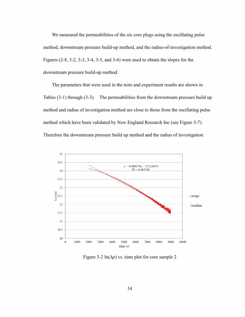
We measured the permeabilities of the six core plugs using the oscillating pulse
method, downstream pressure build-up method, and the radius-of-investigation method.
Figures (2-8, 3-2, 3-3, 3-4, 3-5, and 3-6) were used to obtain the slopes for the
downstream pressure build-up method.
The parameters that were used in the tests and experiment results are shown in
Tables (3-1) through (3-3). The permeabilities from the downstream pressure build up
method and radius of investigation method are close to those from the oscillating pulse
method which have been validated by New England Research Inc (see Figure 3-7).
Therefore the downstream pressure build up method and the radius of investigation
Figure 3-2 ln(∆p) vs. time plot for core sample 2

35
Figure 3-3 ln(∆p) vs. time plot for core sample 3
Figure 3-4 ln(∆p) vs. time plot for core sample 4

36
Figure 3-5 ln(∆p) vs. time plot for core sample 5
Figure 3-6 ln(∆p) vs. time plot for core sample 6

37
method provide reliable ways to estimate permeability of tight rocks.
Traditionally, the oscillating pulse method, which is provided by the Autolab-1500
system, is the fastest way. Figure 3-1 shows that although the measured time of the
oscillating pulse method is only from point ‘A’ to ‘C’, this method still requires the
system to reach the equilibrium state, which can be quite time consuming.
Table 3-1 Permeability measured by oscillating pulse method
Parameter unit Core 1 Core 2 Core 3 Core 4 Core 5 Core 6
k µd 0.108 0.046 0.0724 0.0438 0.11 2.25
Table 3-2 Permeability measured by downstream pressure build-up method
unit Core 1 Core 2 Core 3 Core 4 Core 5 Core 6
L in 2.7780 2.7224 2.7008 2.3882 2.6992 2.5819
D in 1.0311 1.0394 1.0327 1.0323 1.0291 1.0315
φ fraction 0.044 0.045 0.032 0.035 0.036 0.054
cs 1/psi 0.000009 0.000009 0.000009 0.000009 0.000009 0.000009
cg 1/psi 0.000125 0.000125 0.000125 0.000125 0.000125 0.000125
ct 1/psi 0.000134 0.000134 0.000134 0.000134 0.000134 0.000134
μ cp 0.0293 0.0293 0.0293 0.0293 0.0293 0.0293
V2 ft3
2.22E-05 2.22E-05 2.22E-05 2.22E-05 2.22E-05 2.22E-05
s Ln(psi2)/h -2.781108 -1.3644 -1.818 -1.2528 -2.4228 -78.12
k µd 0.1864 0.09 0.1164 0.0791 0.158 5.2731

38
Moreover, the oscillating pulse method is inconvenient. Not only does the range of
the frequency but also the shape of the sine wave need to be chosen carefully, in order to
match the range of the permeability. Choosing the wrong frequency will lead to the
failure in the experiment. Thus, the oscillating pulse method from the Autolab-1500
may not be the optimum option for measuring the low permeability.
The pressure build-up method, which is based on the pulse decay method, is the
transformation of a mature technique to measure the low permeability. Our study
Table 3-3 Permeability measured by radius-of-investigation method
unit Core 1 Core 2 Core 3 Core 4 Core 5 Core 6
L in 2.7780 2.7224 2.7008 2.3882 2.6992 2.5819
φ fraction 0.044 0.045 0.032 0.035 0.036 0.054
cs 1/psi 0.000009 0.000009 0.000009 0.000009 0.000009 0.000009
cg 1/psi 0.000125 0.000125 0.000125 0.000125 0.000125 0.000125
ct 1/psi 0.000134 0.000134 0.000134 0.000134 0.000134 0.000134
μ cp 0.0293 0.0293 0.0293 0.0293 0.0293 0.0293
t h 0.1111 0.28 0.13889 0.14167 0.05556 0.0035
k µd 0.158 0.0615 0.0868 0.0728 0.2438 5.3546

m
op
al
du
sl
D
un
an
a
th
Fig
managed to re
peration tim
lternative of
uring this pr
lope, s, shou
Doing so ensu
ncertainty in
The radiu
nd results in
certain med
he low perm
gure 3-7 Com
educe the do
me. It requir
f the stable an
rocedure, to
uld be part of
ures the con
n the obtaine
us-of-investi
n a reliable an
dia to calcula
eability beco
mparison of
ownstream v
res less time
nd commonl
reduce the u
f the data be
sistency of t
ed permeabil
igation meth
nswer. It u
ate the perme
ome a reality
39
permeabiliti
volume as mu
e than the osc
ly accepted m
uncertainty, t
etween point
the calculatio
lity.
hod requires
utilizes the pr
eability. Th
y in the labo
ies measured
uch as possi
cillating puls
method. It
the data that
t ‘B’ and ‘A’
on of slope,
the least am
ropagation s
his method m
ratory. The
d by three m
ible in order
se method an
t is worth me
are chosen t
in Figure 2-
s, and reduc
mount of the t
speed of the
made a fast m
e measure ti
methods
to reduce th
nd is a faster
entioning tha
to calculate
-9 and Figur
ces the
time to perfo
pressure wa
measuremen
ime for this
he
r
at
the
re 3-1.
orm
ave in
nt of

40
method is 10 times less than the pressure build-up method in our study. Not only the
radius-of-investigation method can be used to measure the low permeability, it can also
be used to measure the high permeability by replacing the gas fluid with the liquid fluid.
Other than the human introduced random error, the major uncertainty source in this
method is mainly from the selection of point ‘B’. In this method, the beginning of the
responding time is manually selected. However, selection of point ‘B’ can be done by
comparing the slopes between the nearby measurements and selecting the largest
changing rate of these slopes. In order to automate the analyzing procedures, this job
needs to be done as part of the future works.
In radius-of-investigation method, we used gas fluid instead of the liquid fluid to
measure low permeability rock. It should be noted that liquid will be used for high
permeability rocks. Replacing gas with liquid, we can still derive the same governing
equations as Equations (2-35) and (2-36) with liquid properties replacing gas properties.
Therefore, Equations (2-35) and (2-36) are capable of estimating permeability of any rock
that meets the aforementioned assumptions. They evaluate the permeability under
unsteady-state flow and require shorter time comparing with other methods.

41
CHAPTER IV
CONCLUSIONS
In this study, we developed two methods to measure the low permeability in the tight
rock, namely the pressure build-up method and the radius-of-investigation method. The
derivation processes were presented and the results from the two measurements were
shown and compared. Our results show that both methods have the capability of
measuring the low permeability and one of them can obtain the measurement in a very
short amount of the time. The key conclusions of our study are listed below:
1). The pressure build-up method was developed based on the pulse decay method,
which is the most commonly used method to measure the low permeability.
2). The radius-of-investigation method was developed using the delayed responding
time from the beginning time that the pressure disturbance entered the sample to the time
that the pressure disturbance propagates to the end of the sample.
3). Both methods provide reliable measurements of the permeability in our study.
4). The radius-of-investigation method can make the measurements within a very
short period of the time, which is 10 times less than that of the commonly used pulse

42
decay method in our experiment.

43
REFERENCES
Al_Hussainy, R., Ramey, H. J., & Crawford, P. B. (1966). The Flow of Real Gases
Through Porous Media. Journal of Petroleum Technology, P624-636.
Billiotte, J., Yang, D., & Su, K. (2008). Experimental study on gas permeability of
mudstones. Physics and Chemistry of the Earch 33, P S231-S236.
Brace, W. F., Walsh, J. B., & Frangos, W. T. (1968). Permeability of Granite under High
Pressure. Journal of Geophysical Research, P2225-2236.
Carlaw, H. S., & Jaeger, J. C. (1959). Conduction of Heat in Solids, second edition.
Oxford at Clarendon Press, P50.
Cui, X., Bustin, A., & bustin, R. M. (2009). Measurement of gas permeability and
diffusivity of tight reservoir rocks: different approaches and their applications.
Geofluids 9, P208-223.
Dicker, A. I., & Smits, R. M. (1988). A Practical Approach for Determining Permeability
From Laboratory Pressure-Pulse Decay Measurements. SPE 17578, P285-292.
Fischer, G. J., & Paterson, M. (1992). Chapter 9 Measurement of Permeability and
Storage Capacity in rocks during Deformation at High Temperature and Pressure.
International Geophysics, V51, P 213-252.

44
Hildenbrand, A., Schlomer, S., & Krooss, B. M. (2002). Gas breakthrough experiments
on finegrained sedimentary rock. Geofluids 2, P3-23.
Hildenbrand, A., Schlomer, S., Krooss, B. M., & Littke, R. (2004). Gas breakthrough
experiments on pelitic rocks: comparative study with N2, CO2 and CH4.
Geofluids 4, P61-80.
Homand, F., Giraud, A., Escoffier, S., & Hoxha, D. (2004). Permeability determination of
a deep argillite in saturated and partially saturated conditions. Int. J. Heat Mass
Transer 47, P3517-3531.
Hsieh, P. A., Tracy, J. V., Neuzil, C. E., Bredehoeft, J. D., & Silliman, S. E. (1981). A
transient laboratory method for determining the hydraulic properties of 'tight'
rocks-I. Theory. International Journal of Rock Mechanics and Mining Sciences &
Geomechanics Abstracts, 18, P245-252.
Jones, S. C. (1997). A Technique for Faster Pulse-Decay permeability Measurements in
Tight Rocks. SPE 28450.
Kranz, R. L., Saltzman, J. S., & Blacic, J. D. (1990). Hydraulic diffusivity measurements
on laboratory rock samples using an oscillating pore pressure method.
International Journal of Rock Mechanics and Mining Sciences & Geomechanics
Abstracts 27, P 345-352.

45
Law, B. E., & Spencer, C. W. (1993). Gas in tight reservoirs-an emerging major source of
energy. The Future of Energy Gasses, US Geological Survey, Professional
Paper1570, P233-252.
Le Guen, C., Deveughele, M., Billiotte, J., & Brulhet, J. (1993). Gas permeability
changes of rocksalt subjected to thermo-mechanical stresses. Quarterly Journal of
Engineering Geology and Hydrogeology, P327-334.
Lee, w. J. (1982). Well Testing. SPE Text book Series V1, P13-15.
Luffel, D. L., Hopkins, C. W., & SchettlerJr., P. D. (1993). Matrix Permeability
Measurement of Gas Productive Shales. SPE26633 Annual Technical Conference
and Exhibition, 3-6 October 1993, Houston, Texas.
Metwally, Y. M., & Sondergeld, C. H. (2011). Measuring low permeabilities of gas-sands
and shales using a pressure transmission technique. International Journal of Rock
Mechanics & Mining Sciences, 1135-1144.
Passey, Q. R., Bohacs, K. M., Esch, W. L., Klimentidis, R., & Sinha, S. (2010). From
Oil-Prone Source Rock to Gas-Producing Shale Reservoir - Geologic and
Petrophysical Characterization of Unconventional Shale Gas Reservoirs.
SPE131350 International Oil and Gas Conference and Exhibition in China, 8-10
June 2010, Beijing, China.

46
Tinni, A., Fathi, E., Agarwal, R., Sondergeld, C., Akkutlu, Y., & Rai, C. (2012). Shale
Permeability Measurements on Plugs and Crushed Samples. SPE 162235
Canadian Unconventional Resources Conference, 30 October-1 November 2012,
Calgary, Alberta, Canada.
Triab, D., & Donaldson, E. C. (2004). Petrophysics (second edition): Theory and Practic
of Measuring Reservoir Rock and Fluid Transport Properties. Amesterdam: Gulf
Professional publishing.

47
NOMENCLATURE
A : area of the cross section of the core plug
cS : formation compressibility
cg : gas isothermal compressibility
ct : total compressibility
D : diameter of core
k : permeability
L : length of core
M : molecular weight
m(p) : gas pseudopressure
Q : the strength of the instantaneous pressure disturbance
p : pressure
pb : base pressure
P2 : downstream pressure
p1 : upstream pressure
Δp : pressure difference
qg : gas rate
R : universal gas constant

48
s : the slope of the pressure difference in a logarithm as a function of time
T : temperature
t : time
tm : time at which the pressure disturbance is a maximum at x
Δt : time period
V1 : volume of the upstream reservoir
V2 : volume of the downstream reservoir
Vp : pore volume of the core
vx : gas velocity in x direction
x : distance from original point in x direction
Δx : incremental distance in x direction
z : gas z-factor
: porosity
ρg : gas density
µ : viscosity
µg : gas viscosity