CONSTANT-PRESSURE MEASUREMENT OF STEAM-WATER RELATIVE ... · Measurement of Steam-Water Relative Permeability ... Figure 5.6: Relative permeability, ... CONSTANT-PRESSURE MEASUREMENT

SGP-TR-169

Constant-PressureMeasurement of Steam-

Water Relative Permeability

Peter A. O’Connor

June 2001

Financial support was provided through theStanford Geothermal Program under

Department of Energy Grant No. DE-FG07-95ID13370and No. DE-FG07-99ID13763,

and by the Department of Petroleum Engineering,Stanford University

Stanford Geothermal ProgramInterdisciplinary Research inEngineering and Earth SciencesSTANFORD UNIVERSITYStanford, California

Abstract

A series of steady-state experiments have established relative permeability curves for

two-phase flow of water in a porous medium. These experiments have minimized

uncertainty in pressure, heat loss, and saturation. By attempting to maintain a constant

pressure gradient, the experiments have provided a baseline from which to determine the

effect of temperature on relative permeability.

The use of a flexible heater with an automatic control system made it possible to assume

negligible phase change for the mobile fluid. X-ray computer tomography (CT) aided by

measuring in-situ steam saturation more directly. Mobile steam mass fraction was

established by separate steam and water inlets or by correlating with previous results.

The measured steam-water relative permeability curves assume a shape similar to those

obtained by Corey (1954) for the simultaneous flow of nitrogen and water. Close

agreement between the curves by Satik (1998), Mahiya (1999), and this study establishes

the reliability of the experimental method and instrumentation adopted in these

experiments, though some differences may bear further investigation. In particular, the

steam phase relative permeability appears to vary much more linearly with saturation

than does the water phase relative permeability.

Acknowledgement

This research was conducted with financial support through the Stanford Geothermal

Program under Department of Energy Grant No. DE-FG07-99ID13763.

The contributions of the following individuals are much appreciated:

Glenn Mahiya, for establishing a sound experimental basis and providing information on

procedure.

Dr. Kewen Li, for frequent consultation on all facets of the experiment theoretical and

practical, and for invaluable experience, knowledge, and insights.

Will Whitted, for truly exceptional technical expertise and assistance in design,

construction, and redesign of all the components of this experiment.

Dr. Roland Horne, for patiently providing direction and motivation in the course of this

research work.

Table of Contents

1. Introduction ................................................................................................................. 4

2. Background ................................................................................................................. 5

2.1. Relative permeability .............................................................................................. 52.2. Saturation ................................................................................................................ 72.3. Slip factor ................................................................................................................ 82.4. Overview of previous results................................................................................... 8

3. Experimental Design ................................................................................................. 10

3.1. General design and apparatus................................................................................ 103.2. Data acquisition system......................................................................................... 123.3. Flexible heaters and control protocol .................................................................... 133.4. CT scanner............................................................................................................. 143.5. Suggested future design modifications ................................................................. 14

4. Experimental procedure ............................................................................................ 17

4.1. General procedure ................................................................................................. 174.2. Constant pressure gradient .................................................................................... 184.3. Procedural limitations ........................................................................................... 18

5. Experimental results and discussion ......................................................................... 20

5.1. General Results ..................................................................................................... 205.2. Saturation .............................................................................................................. 205.3. Correlation between mobile and in-place saturation............................................. 225.4. Pressure ................................................................................................................. 245.5. Temperature .......................................................................................................... 265.6. Heat flux................................................................................................................ 285.7. Relative permeability ............................................................................................ 285.8. Data analysis methods........................................................................................... 305.9. Comparison to previous results ............................................................................. 36

6. Conclusion................................................................................................................. 37

References ......................................................................................................................... 39

A. CT Values.................................................................................................................. 40

B. Data and Calculations................................................................................................ 43

Table of Figures

Figure 3.1: Experimental design schematic. 11

Figure 3.2: Photograph of core assembly mounted on CT scanner couch. 11

Figure 3.3: Flexible heat guard design. 14

Figure 5.1: Saturation profiles. 21

Figure 5.2: Correlation of saturation with inlet quality. 23

Figure 5.3: Pressure profiles. 25

Figure 5.4: Temperature profiles. 27

Figure 5.5: Relative permeability, all data points. 32

Figure 5.6: Relative permeability, interior data points, 15 psi pressure drop. 33

Figure 5.7: Relative permeability, harmonic means. 34

Figure 5.8: Relative permeability, constant saturation and 15 psi pressure drop. 35

Figure 5.9: Comparison of results with previous experiments. 36

4

1. Introduction

Single-phase fluid flow through porous media is normally modeled by Darcy’s Law. To

apply Darcy’s Law to multiphase flow requires the addition of the concept of relative

permeability, which accounts for effects on the flow behavior of one fluid or phase

caused by the presence of another fluid or phase. Relative permeability is believed to

depend primarily on the volume occupied by a phase and so is expressed as a function of

saturation. Potentially reducing effective permeability by an order of magnitude in some

cases, relative permeability can have a dramatic effect on fluid flow and thus is an

important parameter to determine in reservoir engineering. The relative permeability

relations involving oil, water, and gas are well known and have been established in

laboratory experiments. These curves have been used successfully in flow modeling for

petroleum reservoir engineering.

Geothermal reservoirs engineers are necessarily concerned with the flow of steam and

water; steam-water relative permeability curves have been difficult to produce due to the

inherent phase changes between the fluids and the uncertainty of determining water

saturation. A series of experiments conducted by the Stanford Geothermal Program have

sought to establish steam-water relative permeability relations; these experiments have

maintained near-adiabatic steady-state conditions, determined saturation through X-ray

computer tomography, and accounted for slip factor and capillary end effects.

The current work followed on results obtained previously. The objective was to remove

any potential effect of temperature on relative permeability by maintaining a constant

pressure and temperature gradient for every stage of the experiment. Further, the high

pressure gradient should give more reliable and reproducible results with less error than a

low pressure gradient. The results were compiled and analyzed by several methods,

presenting a comprehensive data set.

5

2. Background

2.1. Relative permeability

Relative permeability describes the effect of one fluid or phase on the flow behavior or

another fluid or phase. Fluids interfere with each other by occupying pore volume,

limiting connectivity, and causing effects of interfacial tension. These effects can be

measured quantitatively and determined by including a relative permeability parameter,

which is the permeability to a given fluid of a porous medium partially saturated with

another fluid. Relative permeability is expressed as a ratio of this permeability over the

medium’s measured absolute permeability, and so generally is a number between 0 and 1.

Relative permeability is primarily a function of saturation but could also have some

dependence on temperature, pressure, or flow rate. For multiphase flow of steam and

water the mass flux for each phase is not constant since one phase can be readily

transformed to the other. The current experiment has been designed to minimize phase

changes by maintaining adiabatic conditions.

Relative permeability relations for oil, gas, and water have been used extensively in

petroleum reservoir engineering, but steam-water curves are not as well established. The

curves developed by Corey (1954) for gas-oil relative permeability, and the simpler linear

relations (“X-curves”), are the most commonly used forms of relative permeability

relations.

The Stanford Geothermal Program has conducted many experiments to determine steam-

water relative permeability relations. The experimental procedure has been developed

and enhanced over time to ensure greater accuracy and more rigid experimental controls.

These experiments have found linear curves in some cases and Corey-type curves in

others. Steam relative permeability has been seen to be a more linear function of

saturation than is water relative permeability, though the apparent magnitude of this

difference has varied.

6

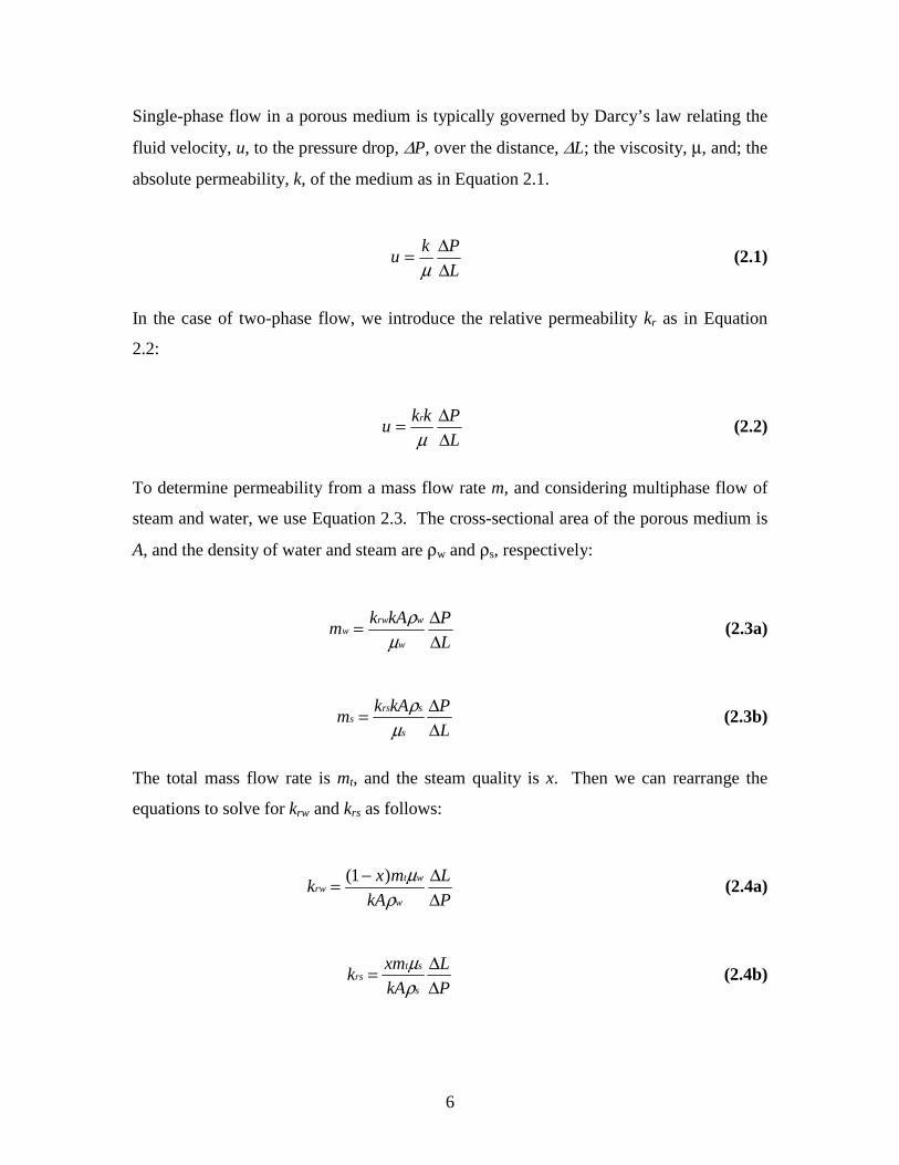
Single-phase flow in a porous medium is typically governed by Darcy’s law relating the

fluid velocity, u, to the pressure drop, ∆P, over the distance, ∆L; the viscosity, µ, and; the

absolute permeability, k, of the medium as in Equation 2.1.

L

Pku

∆∆=

µ(2.1)

In the case of two-phase flow, we introduce the relative permeability kr as in Equation

2.2:

L

Pkku

r

∆∆=

µ(2.2)

To determine permeability from a mass flow rate m, and considering multiphase flow of

steam and water, we use Equation 2.3. The cross-sectional area of the porous medium is

A, and the density of water and steam are ρw and ρs, respectively:

L

PkAkm

w

wrww

∆∆=

µρ

(2.3a)

L

PkAkm

s

srss

∆∆=

µρ

(2.3b)

The total mass flow rate is mt, and the steam quality is x. Then we can rearrange the

equations to solve for krw and krs as follows:

P

L

kA

mxk

w

wtrw

∆∆−=

ρµ)1(

(2.4a)

P

L

kA

xmk

s

strs

∆∆=

ρµ

(2.4b)

7

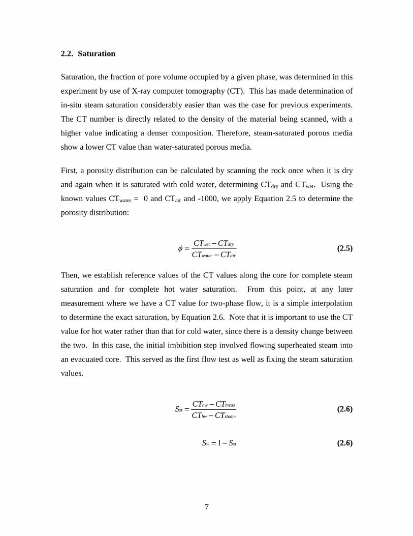
2.2. Saturation

Saturation, the fraction of pore volume occupied by a given phase, was determined in this

experiment by use of X-ray computer tomography (CT). This has made determination of

in-situ steam saturation considerably easier than was the case for previous experiments.

The CT number is directly related to the density of the material being scanned, with a

higher value indicating a denser composition. Therefore, steam-saturated porous media

show a lower CT value than water-saturated porous media.

First, a porosity distribution can be calculated by scanning the rock once when it is dry

and again when it is saturated with cold water, determining CTdry and CTwet. Using the

known values CTwater = 0 and CTair and -1000, we apply Equation 2.5 to determine the

porosity distribution:

airwater

drywet

CTCT

CTCT

−−=φ (2.5)

Then, we establish reference values of the CT values along the core for complete steam

saturation and for complete hot water saturation. From this point, at any later

measurement where we have a CT value for two-phase flow, it is a simple interpolation

to determine the exact saturation, by Equation 2.6. Note that it is important to use the CT

value for hot water rather than that for cold water, since there is a density change between

the two. In this case, the initial imbibition step involved flowing superheated steam into

an evacuated core. This served as the first flow test as well as fixing the steam saturation

values.

steamhw

meashwst

CTCT

CTCTS

−−= (2.6)

stw SS −= 1 (2.6)

8

2.3. Slip factor

Gases flowing under pressure experience a higher effective permeability than liquids do;

the permeability of a porous medium measured by flowing single phase gas varies with

the average pressure in the medium. This effect is known as Klinkenberg effect, and it is

accounted for by correcting gas relative permeability with a slip factor. The correction is

shown in Equation 2.7, where b is a value of 6.58 psia as determined by Li and Horne

(1999).

( )m

rscorrectedrs

pb

kk

+=

1)( (2.7)

2.4. Overview of previous results

As mentioned, relative permeability experiments at Stanford have been progressing for

several years with successive improvements to the apparatus and procedure. The

effectiveness of the experimental procedure was greatly increased with the employment

of a CT scanner to determine steam saturation (Clossman and Vinegar, 1988). The recent

experiments most carefully considered were those of Ambusso (1996), Satik (1998), and

Mahiya (1999). Each experiment introduced new controls and mechanisms to ensure

optimal experimental conditions and accuracy. Ambusso (1996) employed real-time

measurement of temperature and pressure to determine the status of the core at several

points along the core. Ambusso conducted his experiments at a range of temperature and

pressure gradients. Temperature at the first core thermocouple ranged from 101 °C to

117 °C. The fluid was injected in two-phase flow by heating it under pressure and then

flowing it through a throttle valve. Ambusso (1996) determined an X-curve relationship

between relative permeability and saturation. Experiments by Satik (1998) changed the

inlet mechanism, adding separate inlets for steam and for water. Mobile steam quality

was calculated on the basis of separate inlet fluid flows and measured heat flux out of the

core. A new core was prepared, with a core holder of high-temperature plastic. Satik’s

9

results indicated a Corey-type curve relationship for steam-water relative permeability,

with a steam residual saturation of less than 10% and a water residual saturation of 30%.

A subsequent experiment by Mahiya (1999) solved the problem of phase changes with

the addition of a flexible heat guard. This maintained adiabatic conditions throughout the

experiment. Mahiya’s experiment relied on a combination of separate inlets and enthalpy

calculations to determine the steam quality. Generally, mobile saturation during the

imbibition steps could be determined by maintaining single-phase flow from each inlet,

while some of the high-water-saturation drainage steps required mixed flow from each

inlet with the actual mobile saturation estimated from enthalpy. Mahiya’s results

generally agreed with Satik’s, though the steam relative permeability values were slightly

higher and the intersection of steam and water relative permeability was at Sw = .65 rather

than Sw = .55. Mahiya also concluded that there was a Corey-type relationship.

10

3. Experimental Design

The experimental design used in this experiment built on the advances in procedure and

apparatus developed in the previous experiments.

3.1. General design and apparatus

The experiment determined the steam-water relative permeability for a Berea sandstone

core. This was the same core used in experiments by Satik (1998), Mahiya (1999), and

Belen (1999). The core had the following properties: length 43 cm, diameter 5.04 cm,

measured porosity 24%, and permeability 1200 md. Clays in the core were deactivated in

previous experiments by baking it at 800 °C, and the core was cemented with epoxy to a

core holder of high-temperature plastic.

Pressure ports were drilled through the core holder at fixed intervals; heat-resistant plastic

tubing ran from these ports to a pressure transducer box. At these ports, as well as the

inlets and outlets, the pressure tubings were fitted with T-type thermocouples. There

were eight pressure and temperature measurements along the core, two at the inlets, and

one at the outlet. A flexible heat guard, described in Section 3.3, was wrapped around the

core holder. A heat flux sensor was fixed under every section of the heat guard, sending

both heat flux and temperature data to the system. As these sensors were outside the core

holder, they did not register the interior core temperature as accurately as did the

thermocouples at the pressure ports. The whole core was wrapped with insulating fiber

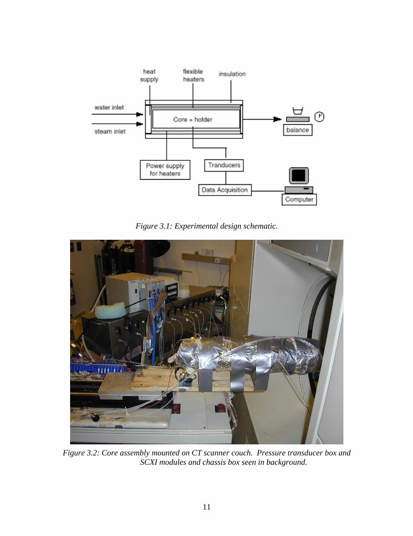
on top of the heat guard to further minimize heat loss. A schematic of the apparatus is

shown in Figure 3.1, and a photograph is shown in Figure 3.2.

11

Figure 3.1: Experimental design schematic.

Figure 3.2: Core assembly mounted on CT scanner couch. Pressure transducer box andSCXI modules and chassis box seen in background.

12

The outlet end piece was plastic, fitted with a pressure port and thermocouple. The inlet

end piece was stainless steel, fitted with two pressure ports and thermocouples, one for

the steam inlet and one for the hot water inlet. A thermal switch was installed within the

end piece to deactivate the furnaces in the event the end piece temperature exceeded 170

°C. This was added to prevent damage to the core in the event of interruption of water

flow to the heaters, as had happened in previous experimental attempts.

Deionized distilled water was sent to a boiler, where it was deaerated. The boiling water

was then pumped through a cooling tank to enable it to pass through the displacement

pump and into the inlet end piece. Two resistance heaters heated the water either to

liquid just below the saturation temperature or to vapor just above the saturation

temperature, and the fluids then entered the core and mixed. A tube ran from the outlet to

a collecting flask on a scale, where the outlet mass flow rate could be measured and

compared to the inlet mass flow rate to determine if the system was at steady state.

3.2. Data acquisition system

We recorded pressures, temperatures, and heat fluxes with a data acquisition system

designed for previous experiments. This system utilized several National Instruments

devices to process a considerable amount of data simultaneously and display it in an

easily readable format on a PC. Signals from the transducers, thermocouples, and heat

flux sensors were sent through a patch board to SCXI-1100 modules, and these modules

were installed in a SCXI-1000 chassis box. The chassis box sent the data to a PC, where

the data was displayed. The PC ran the National Instruments program LABVIEW

version 4.1, a graphical programming utility for instrumentation. LABVIEW provided a

means of monitoring heat flux, temperature, and pressure simultaneously, as well as

controlling the flexible heaters. LABVIEW did not monitor the flow rates or furnace

settings directly, but these could be entered manually so that they would be saved with

the pertinent data. We reconfigured previous LABVIEW routines to suit the needs of this

experiment.

13

3.3. Flexible heaters and control protocol

A flexible heat guard consisting of 18 independent heating elements was wrapped around

the core. A schematic is shown in Figure 3.3. The flexible heaters were connected

through a step-down transformer to a variable output power supply. A LABVIEW

routine was redesigned to activate the heater units as necessary to maintain a constant

heat flux of near zero. To control the individual heaters, we used National Instruments’

SCXI 1163-R module, consisting of 32-channel optically isolated digital output/solid-

state relays. In the closed state, each relay had a maximum resistance of 8 ohms and

carried up to 200 mA of current. A LABVIEW algorithm was constructed to monitor the

heat flux and adjust the heaters as necessary to maintain adiabatic conditions. As the

relays are not variable voltage controllers but simple on/off switches, the necessary heat

flux was generated by setting a duty cycle to each relay, and thus to each heater. A duty

cycle of 0% corresponded to relay being closed and the heater operating all the time,

while a duty cycle of 100% corresponded to the relay remaining open and the heater

being inactive. A cycle in between would open the relay a percentage of the time equal

to the duty cycle during each period. The heaters were generally set to a cycle period of

2-3 seconds, and the ideal power setting was to have most of the duty cycles near 50%.

The control protocol checked the heat flux every minute. If the heat flux for a specific

heater was outside the tolerance range, usually 30 W/m2, the program would increase or

decrease the duty cycle accordingly by a given increment, typically 5%. Due to PC speed

and memory constraints, this protocol often failed to work properly when the graphical

displays were active. For this reason, the control protocol was allowed to establish the

correct heater settings for adiabatic conditions, then the duty cycle increment was set to

0% and the graphical displays were activated. If the heat flux averages left the tolerance

range, the control protocol would be reengaged to adjust as needed. In some cases, when

specific heat flux sensors failed to function adequately, the duty cycle of a given heater

would be set manually to equal that of the heaters on either side and preventing from

adjusting independently.

14

~Digital

Controller

Solid StateRelay

Heater Strip

Heat FluxSensor

Figure 3.3: Flexible heat guard design.

3.4. CT scanner

A modified medical X-ray CT scanner was employed to determine the water saturation at

all points along the core. In-situ saturation values were calculated from images generated

by the Picker Synerview 1200X X-ray CT scanner. The core assembly was mounted and

secured on a couch, which could be controlled by the console on the scanner. The

scanner was equipped with a visible laser and a digital display of the couch position. We

therefore could establish accuracy of the measurement by ensuring that each scan was at

the same relative position along the core for each experiment.

The scanner had been augmented and modified to fit the needs of petroleum and

geothermal reservoir engineering experiments, in particular with the addition of a large

range of variable power settings. This experiment required setting the scanner at 125 kV,

65 mA, an exposure time of 8.49 seconds per slice, and a slice thickness of 10

millimeters. The large slice thickness of the CT scans reduced any potential errors

caused by inaccuracy in the couch positioning system.

3.5. Suggested future design modifications

This experiment provided insight into potential future improvements to the experimental

procedure and apparatus. The data acquisition system is exceptionally useful and should

15

become even more powerful and adaptable with newer versions of LABVIEW. We

suggest employing a faster PC to take full advantage of LABVIEW’s capabilities. The

CT scanner is accurate and provides a clear picture of the interior of the core. The

flexible heat guard greatly enhances the effectiveness of the experiment by negating the

need for heat loss estimations.

The core holder itself could be improved, in particular the inlet end piece. The stainless

steel end piece is resistant to thermal damage and permits the addition of a thermal switch

to prevent damage to the core. However, this particular device creates difficulties in

controlling the steam and water inlets. Excess heat from the steam furnace heats the inlet

water, to the extent that it was often not needed to supply any heat at all to the water

furnace in order to have water at the saturation temperature. Maintaining superheated

steam and liquid water at the two inlets was difficult. At times, the hot water temperature

appeared to exceed the saturation temperature, despite the fact that there was not enough

power going into the core to heat the given flow rate to superheated conditions. This may

have been a consequence of steam pockets forming in the water furnace at the location of

the thermocouple, or asymmetrical water flow around the furnace. In all of these cases,

the temperature at the first pressure port was at the saturation temperature, even if both

steam and water inlets had appeared to be injecting superheated steam. Therefore, it is

not considered that injection through then water inlet was actually superheated steam in

these cases.

The steel end piece also at times heated the water at the first pressure port to a higher

temperature than the water in the inlet. This would be the case when the energy produced

by the heaters could not be entirely transferred to the injected fluids as they passed

through the end piece. This effect is visible in a couple of the temperature profiles in

Section 5, though it was often a problem that had to be fixed during the experiment. If,

as a consequence of heat transfer between the furnaces, there was more steam entering

the core than was entering solely through the steam inlet, we would have underestimated

the steam relative permeability in some cases.

16

A future end piece should retain the stainless steel construction, but should have a greater

separation between the steam furnace and the water furnace. A gap cut down the length

of the endpiece, filled with insulation or left open to the air, would greatly reduce heat

transfer between the steam heater and the water heater. A thermal switch should be

installed in the steam heater side of the inlet, since it will be necessary to deactivate the

heaters in the event of interruption of water supply. Two other methods might allay the

problem of heat transfer between the heaters. Preheating the steam would reduce the

power necessary for the steam furnace, as would the use of external furnaces. The

internal furnaces minimize atmospheric heat loss, an advantage that we may not wish to

dispense with.

The displacement pumps used in this experiment were accurate, but not very reliable. In

one case, loss of fluid flow resulted in damage to the core and warranted the installation

of the thermal switch. After that modification, there were several other flow decreases

that caused temperature spikes and triggered the thermal switch. We suggest replacement

of the displacement pumps.

If the experiment is to be repeated at a different pressure gradient, additional

modifications would be necessary. The current core holder is probably not suitable for

temperature and pressure gradients significantly higher than those used in this

experiment. A titanium core holder might be an effective option if its cost is not

prohibitive.

17

4. Experimental procedure

This section describes the steps taken in the experiment, conceptual goals, and challenges

encountered. The experimental procedure closely followed the procedure established by

Mahiya (1999), though certain changes were made to enhance the effectiveness of the

experiment.

4.1. General procedure

The water supply was set up as detailed in Section 3. The boiler had to be refilled

periodically with water and allowed to boil for a length of time sufficient to deaerate the

water. Once the water was deaerated and the boiler was full and turned off, the system

could generally be allowed to run overnight or for several hours during the day to

establish steady-state conditions. This was not the case for experiments at high mass

flow rate. Outlet water was collected occasionally and weighed on a scale to compare the

outlet mass flow rate to the injection mass flow rate, to verify steady-state conditions and

to confirm the accuracy of the pump flow rates.

The experiment began with an imbibition process. Performing the imbibition process

first allowed determination of the maximum necessary steam flow and correspondingly

the maximum necessary power input. The initial step was a flow of superheated steam

into an evacuated core; as the CT values for this step were actually slightly lower than

those found for the evacuated core, this was used as the baseline for calibration of the CT

values. Therefore, the steam saturation in this step was taken to be 100%, as the

temperature at all points along the core was considerably higher than the saturation

temperatures. Fluid injection continued, with an increasing water mass fraction in each

successive step of the experiment. We attempted to control temperature sufficiently that

there was obviously single-phase flow from each inlet. At each step, after the system had

reached steady-state conditions, a CT scan of the core was taken. The images were

processed on the Picker console, transferred to a magnetic tape drive, and then saved to a

PC.

18

Once the imbibition step was complete, the drainage process began. During this process,

only one inlet pump was available and two-phase fluid was injected at saturated

conditions. Mobile steam quality was calculated as detailed in Section 5.3. The drainage

experiments took place over a range of high and moderate water saturations.

Unfortunately, it was not possible to further investigate the region of low water

saturation.

4.2. Constant pressure gradient

In this experiment, we attempted to maintain a constant pressure gradient of 0.89 psi/inch

(a 15 psi pressure drop over a 43 cm core) to avoid any effects of temperature on relative

permeability. The outlet was at atmospheric pressure, and an inlet pressure of 15 psig

corresponded to a saturation temperature of 120 °C. Constant pressure gradient was to be

maintained by varying the flow rate as needed. Total mass flow rate ranged from 2 g/min

to 16 g/min for all of the steps at the target pressure gradient.

4.3. Procedural limitations

Certain modifications to the experiment were necessitated by limitations of the apparatus.

During the drainage step, hot water was to be injected through one inlet and steam

through another, as had been done in the imbibition step. However, in this stage of the

experiment we sought to produce very small steam flow rates, to further examine the area

of high water saturation. For the flow rates considered, it proved to be impossible to heat

fluid in the steam inlet to superheated conditions without considerable transfer of excess

heat to the core and to the hot water inlet. It proved easier to produce miniscule amounts

of steam by heating the inlet water to the saturation temperature. Later in the drainage

step, it would have been possible to return to a dual-inlet setup, but the other

displacement pump had begun to fail, possibly due to a leaking seal.

The original inlet thermocouples failed and were replaced before the drainage step, but

the replacement thermocouples were less accurate due to difficulties in positioning them

precisely enough. They routinely read temperatures too high (if the thermocouple was

positioned near the heater) or too low (if it was further back along the pressure tubing).

19

In the drainage step, the temperature at the first pressure port was used to determine if the

flowing fluid was at saturated conditions. While it would be better to know the actual

inlet temperature, it was not crucial, as we did not have separate inlets of superheated

steam and liquid water.

Certain of the drainage steps may not have reached steady-state flow. Due to the large

volume of water involved, they could only be left unattended for 2-3 hours at most before

the boiler would need to be refilled; as a consequence, they could not stabilize overnight.

In these cases, they were monitored and as much time as possible was allowed for the

system to stabilize. This most likely accounts for the saturation front seen in some of the

drainage experiments.

20

5. Experimental results and discussion

5.1. General Results

A total of 28 steady-state experiments were performed over a period of several weeks.

The resulting data covered the full range of saturations, with particularly large amounts of

data for regions of moderate saturation. Fifteen imbibition experiments were performed,

followed by 13 drainage experiments. The drainage experiments had greater success in

covering the range of high water saturations but suffered from loss of accuracy in

determining the flowing steam saturation. Near-adiabatic conditions were maintained for

all experiments. Other than an initial flow of 100% steam into an evacuated core, the

maximum steam saturation reached was about 65%. The maximum water saturation

reached was 100%, due to condensation of immobile steam during the earliest drainage

step. The full results of the experiment are presented in Appendix B, in chronological

order.

5.2. Saturation

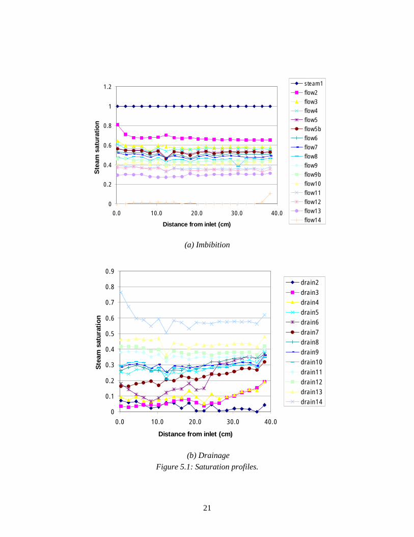
Saturation profiles during the imbibition step, shown in Figure 5.1a, were constant across

the core and cover the range of steam saturation from 30% to 65%. These tests did not

cover a range of high-water or high-steam saturations. The saturation profiles in the

drainage step, shown in Figure 5.1b, exhibit greater variation across the core, but also

covered a wider range of saturations. The existence of a saturation front and multiple flat

saturation regions allowed these experiments to provide useful data. The presence of

fronts in the drainage phase may be the result of unsteady-state conditions, or it may be

the result of the steam in the latter part of the core being more difficult to displace. In

results presented later in this chapter, one relative permeability graph is presented using

the average saturation from the first half of the core, which showed stable saturation at all

points. Capillary end effect was visible in many of the steps. For this reason, one

relative permeability graph is presented excluding the pressure ports nearest to the inlet

and outlet.

21

0

0.2

0.4

0.6

0.8

1

1.2

0.0 10.0 20.0 30.0 40.0

Distance from inlet (cm)

Ste

amsa

tura

tio

n

steam1

flow2

flow3

flow4

flow5

flow5b

flow6

flow7

flow8

flow9

flow9b

flow10

flow11

flow12

flow13

flow14

(a) Imbibition

0

0.1

0.2

0.3

0.4

0.5

0.6

0.7

0.8

0.9

0.0 10.0 20.0 30.0 40.0


Ste

amsa

tura

tion

drain2

drain3

drain4

drain5

drain6

drain7

drain8

drain9

drain10

drain11

drain12

drain13

drain14

(b) Drainage

Figure 5.1: Saturation profiles.

22

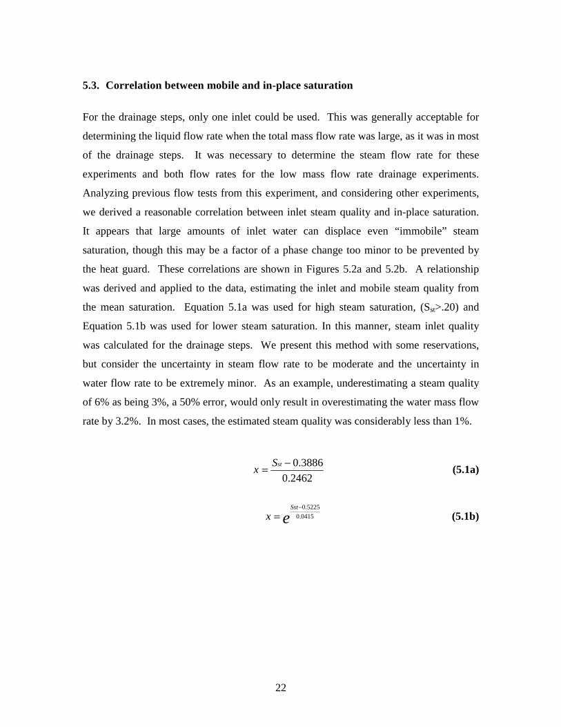
5.3. Correlation between mobile and in-place saturation

For the drainage steps, only one inlet could be used. This was generally acceptable for

determining the liquid flow rate when the total mass flow rate was large, as it was in most

of the drainage steps. It was necessary to determine the steam flow rate for these

experiments and both flow rates for the low mass flow rate drainage experiments.

Analyzing previous flow tests from this experiment, and considering other experiments,

we derived a reasonable correlation between inlet steam quality and in-place saturation.

It appears that large amounts of inlet water can displace even “immobile” steam

saturation, though this may be a factor of a phase change too minor to be prevented by

the heat guard. These correlations are shown in Figures 5.2a and 5.2b. A relationship

was derived and applied to the data, estimating the inlet and mobile steam quality from

the mean saturation. Equation 5.1a was used for high steam saturation, (Sst>.20) and

Equation 5.1b was used for lower steam saturation. In this manner, steam inlet quality

was calculated for the drainage steps. We present this method with some reservations,

but consider the uncertainty in steam flow rate to be moderate and the uncertainty in

water flow rate to be extremely minor. As an example, underestimating a steam quality

of 6% as being 3%, a 50% error, would only result in overestimating the water mass flow

rate by 3.2%. In most cases, the estimated steam quality was considerably less than 1%.

2462.0

3886.0−= stSx (5.1a)

eSst

x 0415.0

5225.0−

= (5.1b)

23

0

0.2

0.4

0.6

0.8

1

1.2

0.0001 0.001 0.01 0.1 1

inlet steam quality

stea

msa

tura

tio

n

(a) Logarithmic plot

0

0.2

0.4

0.6

0.8

1

1.2

0 0.2 0.4 0.6 0.8 1

inlet steam quality

stea

msa

tura

tion

(b) Linear plot

Figure 5.2: Correlation of saturation with inlet quality.

24

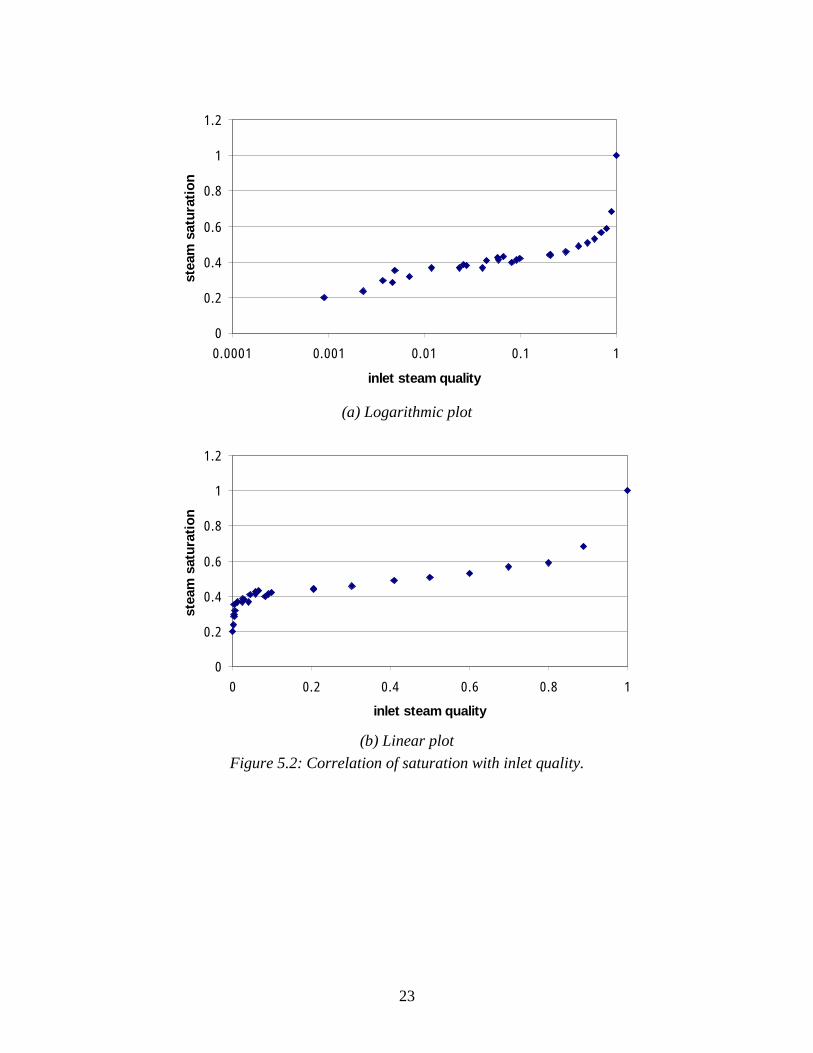
5.4. Pressure

The goal of this experiment was to maintain a constant pressure drop of 15 psi by varying

the flow rate as needed. This was successfully accomplished throughout the entire

imbibition phase, save for the 100% water inlet step at the end. The constant pressure

gradient could not be maintained in a few cases of high water flow, such as the end of the

imbibition phase and the first few trials of the drainage phase. In these cases, the pump

and heater could not supply sufficient water at 120 °C to maintain a 15-psi pressure drop

across the core. For attempts to increase the flow rate further, the main limitation

appeared to be the rate of heat transfer from the water heater to the fluid flowing over it.

The water being injected remained considerably below the saturation temperature, yet the

temperature at the first pressure port was higher than that measured for the hot water

inlet. This indicated that the heater was not transferring all of its heat to the fluid, and

that the excess was transferred directly to the core, which could result in damage to the

core. Pressure profiles are shown in Figure 5.3a and Figure 5.3b. Note that the pressure

drop is very close to 15 psi for most of the drainage steps and all but one of the

imbibition steps.

A second reason to maintain the 15 psi pressure drop is that it appears the transducers are

most reliable in that range. Flow tests at lower pressure seem more likely to have minor

anomalies, which resulted in relative permeability either inflating or becoming negative.

This may simply be a consequence of absolute errors and fluctuations in the pressure

readings, which produce a greater relative effect at low pressure. For this reason, the

flow tests with lowest pressure gradients are excluded from most presentations of the

relative permeability data.

25

0

2

4

6

8

10

12

14

16

18

20

0 10 20 30 40 50


Pre

ssur

e(p

sig)

steam1

flow2

flow3

flow4

flow5b

flow6

flow7

flow8

flow9

flow9b

flow11

flow10

flow12

flow13

flow14

(a) Imbibition

0

2

4

6

8

10

12

14

16

18

0 10 20 30 40 50


Pre

ssur

e(p

sig)

drain2

drain3

drain4

drain5

drain6

drain7

drain8

drain9

drain10

drain11

drain12

drain13

drain14

(b) Drainage

Figure 5.3: Pressure profiles.

26

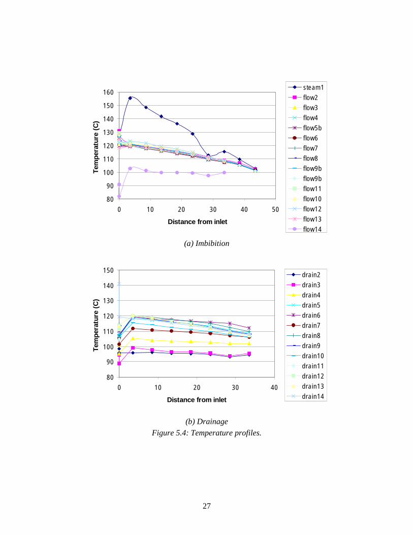
5.5. Temperature

The core temperatures generally matched the saturation temperatures at the measured

pressures. Slight deviations due to instrument inaccuracy and fluctuation existed, so we

took 1 psi to be an acceptable margin of error between the measured temperature and the

saturation temperature. Anything outside of that range was considered superheated or

unsaturated. Some steps, such as the steam imbibition phase, exhibited a higher

temperature at the first pressure port than at the inlet. This was regarded as a

consequence of inadequate heat transfer away from the steam heater, with the result being

that the heater was radiating excess heat through the end piece and into the core. This

was generally not a desirable condition. Temperature profiles are shown in Figure 5.4a

and Figure 5.4b. Note that for much of the drainage phase the thermocouples near the

end of the core were not functional. The more reliable thermocouples from the end of the

core had been moved to replace malfunctioning thermocouples at the inlets, as

controlling the inlet temperature as precisely as possible was of greater importance than

monitoring the outlet temperature.

27

80

90

100

110

120

130

140

150

160

0 10 20 30 40 50

Distance from inlet

Tem

pera

ture

(C)

steam1

flow2

flow3

flow4

flow5b

flow6

flow7

flow8

flow9b

flow9b

flow11

flow10

flow12

flow13

flow14

(a) Imbibition

80

90

100

110

120

130

140

150

0 10 20 30 40

Distance from inlet

Tem

pera

ture

(C)

drain2

drain3

drain4

drain5

drain6

drain7

drain8

drain9

drain10

drain11

drain12

drain13

drain14

(b) Drainage

Figure 5.4: Temperature profiles.

28

5.6. Heat flux

The average heat flux was kept within 30 W/m2 of a target heat flux of 0 W/m2

throughout each experiment. As the individual heaters cycled on and off, the

instantaneous heat flux at any given sensor at a specific time may have been between 80

and -80 W/m2. The instantaneous heat flux data was recorded but is not an effective

measure of the actual heat flux and so is not included here. Two heat flux sensors were

highly erratic, so the heaters for these strips were set to the duty cycles of adjacent

heaters. A recurring concern throughout the experiment was heat flux through the

stainless steel inlet end piece. This prevented the calculation of inlet enthalpy based on

power supplied to the furnaces, which would have otherwise been a useful method to

estimate inlet steam quality.

5.7. Relative permeability

Results for relative permeability appear to be Corey-type curves for water and possibly a

more linear relationship for steam. Maximum steam saturation appears to be around

70%, and maximum water saturation appears to be 90%. When considering the flow

trials not occurring at the target pressure gradient, there are indications that krw may be as

high as 0.65 or even higher. These less-reliable trials comprise nearly all of the cases

with water saturation greater than 0.8, so it might not be appropriate to discard them

entirely.

In all figures other than Figure 5.7 (the harmonic averages), the data from the first

pressure port and the outlet are excluded. Each stage of the experiment showed a

considerable disparity between the data from these ports and the data determined

elsewhere along the core. This was most likely due to capillary end effect or unusual

pressure behavior involving the placement of the inlet and outlet pressure tubings. The

data are presented as follows:

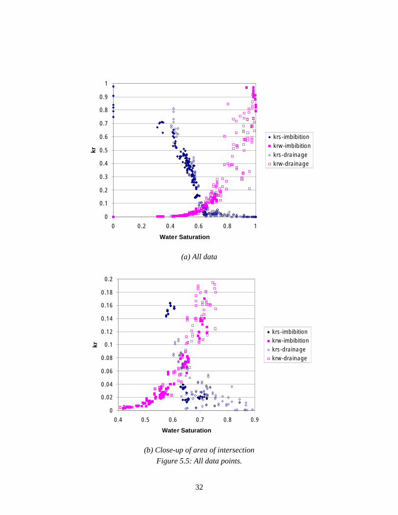
Figures 5.5a and 5.5b show the relative permeability curves for all data points other than

the first pressure port and the outlet. Note that a few data points indicated permeabilities

significantly greater than 1 or less than 0 even after correcting for the slip factor; these

29

were attributed to instrumentation anomalies and were ignored. Figure 5.5b focuses on

the data near the area of low permeability around Sw = 0.64. In this view, we see that the

imbibition steps show scattered clusters of the krs data, rather than any significant trend.

Figures 5.6a and 5.6b show the relative permeability for all points in the interior of the

core (pressure ports 2-7) and the points from flow tests with a gradient less than 12 psi.

This shows a maximum water saturation of 0.92, a maximum steam saturation of 0.69,

and increasing scatter in krw as Sw increases.

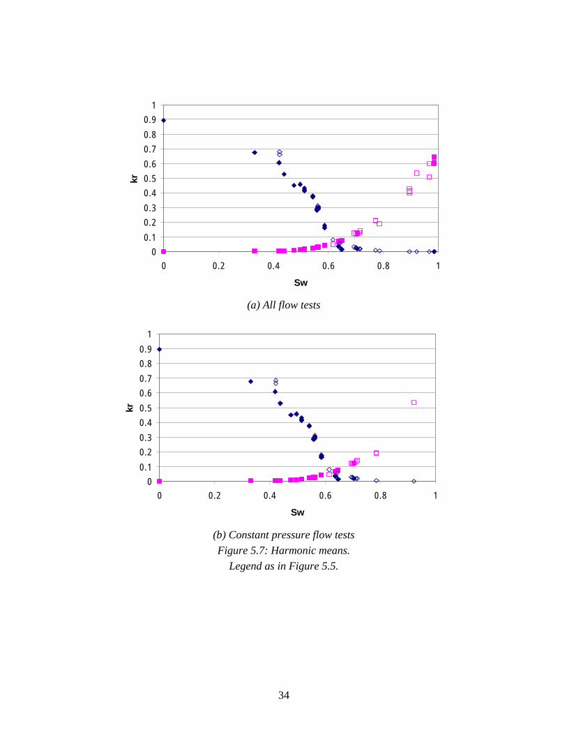
Figures 5.7a and 5.7b show the mean relative permeabilities across the core for each step;

Figure 5.7a shows the mean values from all steps, while Figure 5.7b excludes the runs

which did not occur with a pressure drop near 15 psi.

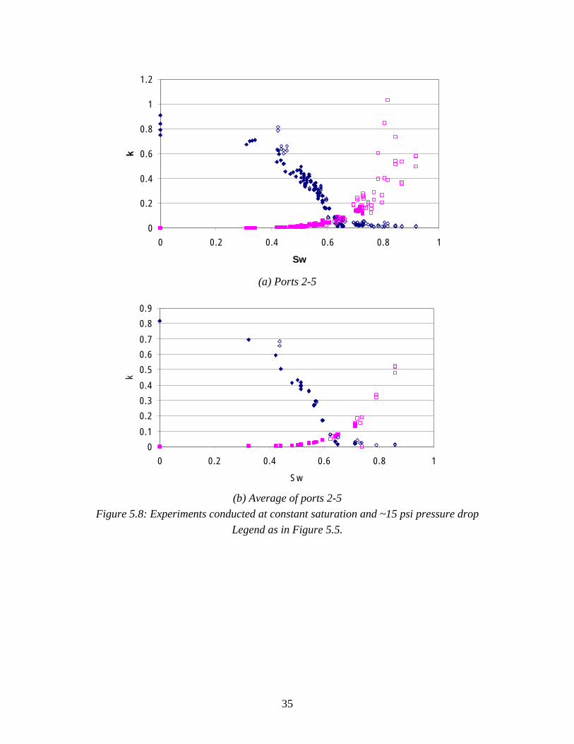
Figures 5.8a and 5.8b show the relative permeability calculated at the data points 2-5,

which had uniform saturation in each flow test and were generally free from anomalous

pressure readings resulting in inflated or negative relative permeability. Figure 5.8a

shows all the data, and Figure 5.8b shows the averaged values for each flow test. These

graphs exclude the flow tests of high water saturation that had a pressure drop of less than

12 psi. The corrections show some improvement in the scatter for the graph of all data

points, but no real change from the harmonic means of the entire core.

Note that there are considerably more data points than there are steady-state experiments;

each experiment allowed determination of relative permeability across every interval

between pressure ports. In addition, some experiments had pressure and temperature data

recorded several times during the 30-minute scanning interval, resulting in multiple

relative permeability values for a single flow test if there was variation in the transducers

or thermocouples.

It is our conclusion that the data from the harmonic means (Figure 5.7a) are the most

reliable and the best representation of the total data gathered. It then appears that while

water relative permeability follows a Corey-type curve similar to that found in previous

experiments, steam relative permeability follows a steeper and more linear trend. This

conclusion does not change when different sections of the data are considered. The

30

steam relative permeability deviates from a Corey curve in several regions, and not

simply for the drainage data points involving a mobile steam quality calculated through

correlations. It may be that steam relative permeability follows a truly different relation,

or it may be that there was some systematic error in the calculation of steam flow rates.

If, for example, the inlet heaters were heating the end piece enough that water was turned

to steam after it passed the inlet thermocouples and entered the core, the result would be

underestimated inlet steam quality. This bears further investigation with particular focus

on the region of water saturation between 50% and 75%.

From the graphs, residual water saturation appears to be around 30%, and residual steam

saturation appears to be around 10%. Residual steam saturation is hard to determine

since the drainage tests began with an initial water saturation of about 100%.

The data points from the low-pressure stages are not consistent with the rest of the data.

This may be due to an actual effect of pressure on relative permeability, but it is more

likely due to two other factors. The low-pressure flow tests are also the flow tests with

highest water saturation, and low pressure gradients are more significantly disturbed by

fluctuations and inaccuracies in the pressure transducers.

5.8. Data analysis methods

The values for mean relative permeability across the core were calculated by taking the

harmonic average of the relative permeabilities for all points along the core, then plotting

against the mean saturation across the core. This accounted for the varying viscosity and

density, whereas averaging the temperature and viscosity and calculating relative

permeability based on the overall pressure drop would not have done so. The data was

originally calculated considering all data points, then considering only the interior data

points (ignoring the data points closest to the inlet and outlet). There was no noticeable

difference in the appearance of the averaged data; while the capillary end effect may

create anomalous outlying points on a graph of all data, these points will not significantly

alter the average of the data. In Figure 5.8b, the same method was used, but only the

values for saturation and relative permeability between ports 2 and 5 were considered.

31

Averaging the saturation across the core does not account for the flow tests in which the

saturation varied across the half of the core nearest the outlet, as was the case for

approximately half of the drainage tests. This problem was to be eliminated by only

considering ports 2 through 5. However, even when the whole core was considered and

averaged, the points from these tests did not diverge from the data trends, as the

relationship between relative permeability and saturation is nearly linear over the

relatively small range of saturation seen in those tests.

Data were also compiled for the relative permeability as measured at each individual

pressure port. The shapes of the relative permeability graph were similar throughout,

though each pressure port had different endpoints. The lack of high water saturation

values in the latter part of the core limited the data available in those sections, and the

graphs overall did not reveal any abnormalities in any of the interior pressure ports.

32

0

0.1

0.2

0.3

0.4

0.5

0.6

0.7

0.8

0.9

1

0 0.2 0.4 0.6 0.8 1

Water Saturation

kr

krs-imbibition

krw-imbibition

krs-drainagekrw-drainage

(a) All data

0

0.02

0.04

0.06

0.08

0.1

0.12

0.14

0.16

0.18

0.2

0.4 0.5 0.6 0.7 0.8 0.9

Water Saturation

kr

krs-imbibitionkrw-imbibitionkrs-drainagekrw-drainage

(b) Close-up of area of intersection

Figure 5.5: All data points.

33

0

0.2

0.4

0.6

0.8

1

1.2

0 0.2 0.4 0.6 0.8 1

Sw

kr

(a) All data

0

0.02

0.04

0.06

0.08

0.1

0.12

0.14

0.16

0.18

0.2

0.4 0.5 0.6 0.7 0.8 0.9

Sw

kr

(b) Close-up of area of intersection

Figure 5.6: Interior data points, 15 psi pressure drop.

Legend as in Figure 5.5.

34

0

0.1

0.2

0.3

0.4

0.5

0.6

0.7

0.8

0.9

1

0 0.2 0.4 0.6 0.8 1

Sw

kr

(a) All flow tests

0

0.1

0.2

0.3

0.4

0.5

0.6

0.7

0.8

0.9

1

0 0.2 0.4 0.6 0.8 1

Sw

kr

(b) Constant pressure flow tests

Figure 5.7: Harmonic means.


35

0

0.2

0.4

0.6

0.8

1

1.2

0 0.2 0.4 0.6 0.8 1

Sw

k

(a) Ports 2-5

0

0.1

0.2

0.3

0.4

0.5

0.6

0.7

0.8

0.9

0 0.2 0.4 0.6 0.8 1

Sw

k

(b) Average of ports 2-5

Figure 5.8: Experiments conducted at constant saturation and ~15 psi pressure drop


36

5.9. Comparison to previous results

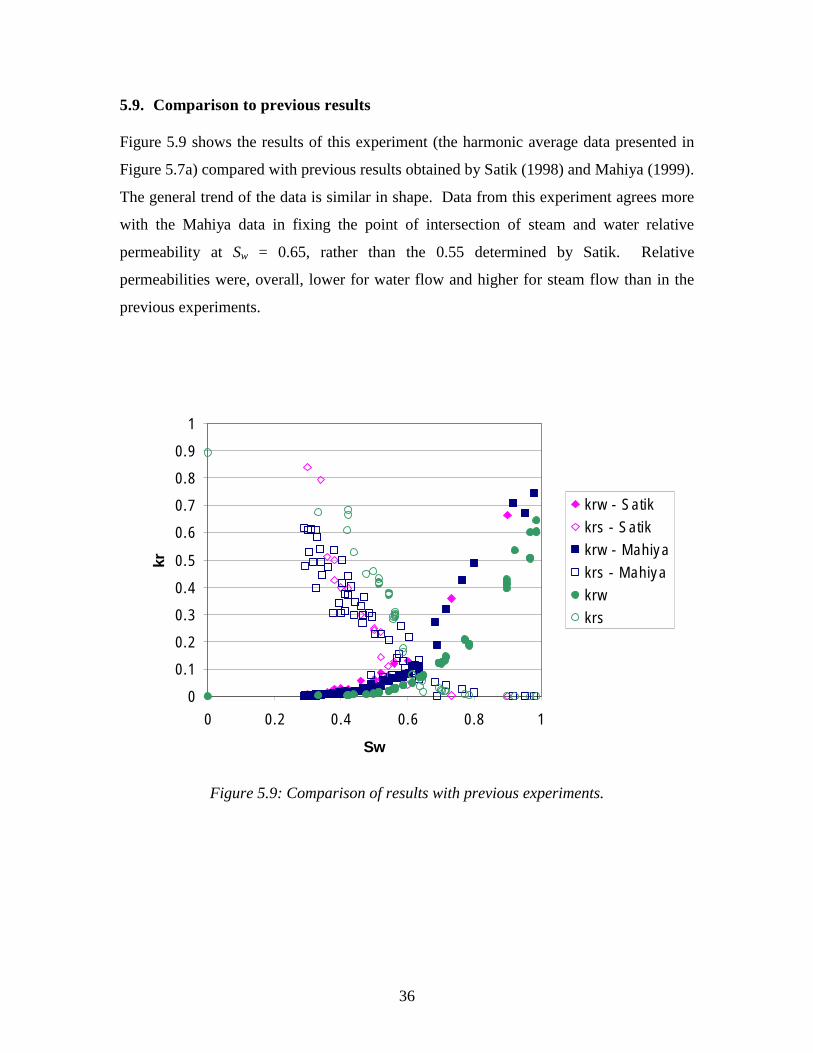
Figure 5.9 shows the results of this experiment (the harmonic average data presented in

Figure 5.7a) compared with previous results obtained by Satik (1998) and Mahiya (1999).

The general trend of the data is similar in shape. Data from this experiment agrees more

with the Mahiya data in fixing the point of intersection of steam and water relative

permeability at Sw = 0.65, rather than the 0.55 determined by Satik. Relative

permeabilities were, overall, lower for water flow and higher for steam flow than in the

previous experiments.

0

0.1

0.2

0.3

0.4

0.5

0.6

0.7

0.8

0.9

1

0 0.2 0.4 0.6 0.8 1

Sw

kr

krw - Satik

krs - Satik

krw - Mahiya

krs - Mahiya

krw

krs

Figure 5.9: Comparison of results with previous experiments.

37

6. Conclusion

This experiment built on the methodology developed in previous experiments to

determine steam-water relative permeability at constant pressure gradient. Heat flux was

controlled successfully to maintain adiabatic conditions within the core, though concerns

remain about excessive heat gain or loss through the inlet. A constant pressure gradient

was maintained in most cases, though maintaining a constant pressure gradient at high

water flow rates continues to be a challenge.

A comprehensive data set was compiled. Pressure, temperature, and saturation were

measured and recorded and used to calculate relative permeability. The data were then

analyzed in a number of ways, and several representations of the steam-water relative

permeability relations were presented.

The relative permeability relations suggested by this study support a Corey-type profile

for water relative permeability, though they suggest otherwise for steam relative

permeability. As in previous experiments, residual water saturation of this core was

found to be in the vicinity of 30%. Residual steam saturation was more difficult to

determine but apparently near 10%. The steam phase slip factor has a significant effect

on the relative permeability. If not considered, it will increase the apparent relative

permeability of the steam phase by 20-40%.

This relative permeability experiment focused on a specific Berea sandstone core under a

pressure gradient of 15 psi across 43 cm, with an inlet temperature of 120 °C. As

geothermal reservoirs tend to be of a composition different than sandstone, with

temperatures in excess of 120 °C, these results are not directly applicable to geothermal

reservoir engineering in their current form. However, they do provide important insights

into the general behavior of steam and water in two-phase flow, which should be similar

in form if not in detail to the flow properties of steam and water under geothermal

38

conditions. The experimental methodology established should prove useful for

expanding this experiment to include geothermal reservoir material.

For the immediate future, it is our hope that subsequent investigations involve similar

experiments at a different pressure gradient, to evaluate the role of pressure and

temperature on relative permeability. Experimentation at a greater pressure gradient may

require the development of a different core holder mechanism, while experimentation at a

lesser pressure gradient may require more sensitive and precise transducers.

39

References

Ambusso, W.J., “Experimental Determination of Steam-Water Relative Permeability

Relations,” MS thesis, Stanford University, Stanford, California (1996).

Clossman, P.J. and Vinegar, J.J., “Relative Permeability to Steam and Water at Residual

Oil in Natural Cores; CT Scan Saturation,” SPE paper 174449.

Corey, A.T., “The Interrelations Between Gas and Oil Relative Permeabilities,”

Producers Monthly Vol. 19 (1954), pp 38-41.

Li, K. and Horne, R.N., “Accurate Measurement of Steam Flow Properties,” GRC

Transactions 23 (1999).

Mahiya, G, “Experimental Measurement Of Steam-Water Relative Permeability,” MS

thesis, Stanford University, Stanford, California (1999).

Satik, C., “A Measurement of Steam-Water Relative Permeability,” Proceedings of 23rd

Workshop on Geothermal Reservoir Engineering, Stanford University, Stanford,

California (1998)

40

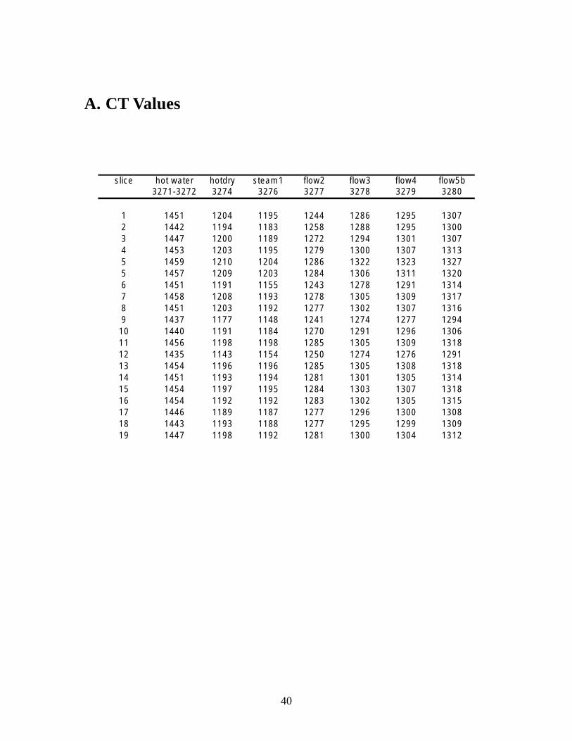
A. CT Values

slice hot water hotdry steam1 flow2 flow3 flow4 flow5b3271-3272 3274 3276 3277 3278 3279 3280

1 1451 1204 1195 1244 1286 1295 13072 1442 1194 1183 1258 1288 1295 13003 1447 1200 1189 1272 1294 1301 13074 1453 1203 1195 1279 1300 1307 13135 1459 1210 1204 1286 1322 1323 13275 1457 1209 1203 1284 1306 1311 13206 1451 1191 1155 1243 1278 1291 13147 1458 1208 1193 1278 1305 1309 13178 1451 1203 1192 1277 1302 1307 13169 1437 1177 1148 1241 1274 1277 129410 1440 1191 1184 1270 1291 1296 130611 1456 1198 1198 1285 1305 1309 131812 1435 1143 1154 1250 1274 1276 129113 1454 1196 1196 1285 1305 1308 131814 1451 1193 1194 1281 1301 1305 131415 1454 1197 1195 1284 1303 1307 131816 1454 1192 1192 1283 1302 1305 131517 1446 1189 1187 1277 1296 1300 130818 1443 1193 1188 1277 1295 1299 130919 1447 1198 1192 1281 1300 1304 1312

41

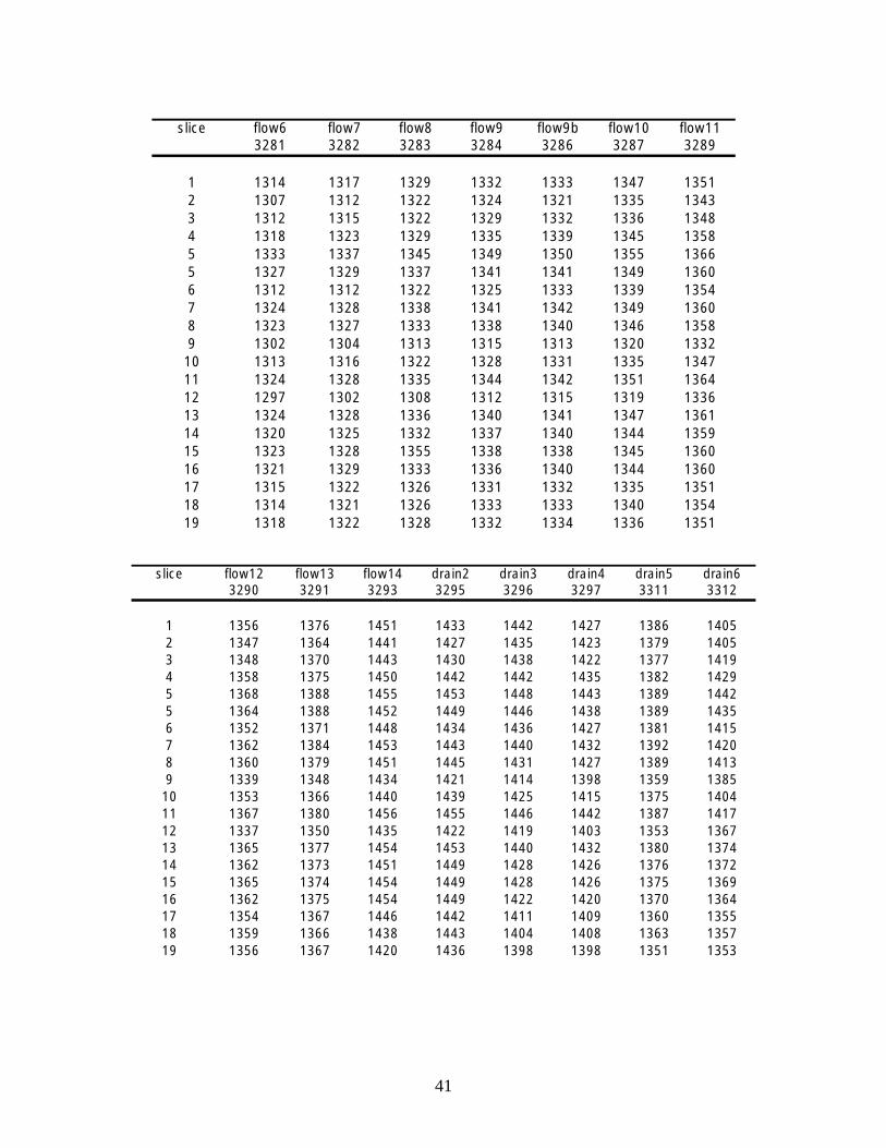
slice flow6 flow7 flow8 flow9 flow9b flow10 flow113281 3282 3283 3284 3286 3287 3289

1 1314 1317 1329 1332 1333 1347 13512 1307 1312 1322 1324 1321 1335 13433 1312 1315 1322 1329 1332 1336 13484 1318 1323 1329 1335 1339 1345 13585 1333 1337 1345 1349 1350 1355 13665 1327 1329 1337 1341 1341 1349 13606 1312 1312 1322 1325 1333 1339 13547 1324 1328 1338 1341 1342 1349 13608 1323 1327 1333 1338 1340 1346 13589 1302 1304 1313 1315 1313 1320 133210 1313 1316 1322 1328 1331 1335 134711 1324 1328 1335 1344 1342 1351 136412 1297 1302 1308 1312 1315 1319 133613 1324 1328 1336 1340 1341 1347 136114 1320 1325 1332 1337 1340 1344 135915 1323 1328 1355 1338 1338 1345 136016 1321 1329 1333 1336 1340 1344 136017 1315 1322 1326 1331 1332 1335 135118 1314 1321 1326 1333 1333 1340 135419 1318 1322 1328 1332 1334 1336 1351

slice flow12 flow13 flow14 drain2 drain3 drain4 drain5 drain63290 3291 3293 3295 3296 3297 3311 3312

1 1356 1376 1451 1433 1442 1427 1386 14052 1347 1364 1441 1427 1435 1423 1379 14053 1348 1370 1443 1430 1438 1422 1377 14194 1358 1375 1450 1442 1442 1435 1382 14295 1368 1388 1455 1453 1448 1443 1389 14425 1364 1388 1452 1449 1446 1438 1389 14356 1352 1371 1448 1434 1436 1427 1381 14157 1362 1384 1453 1443 1440 1432 1392 14208 1360 1379 1451 1445 1431 1427 1389 14139 1339 1348 1434 1421 1414 1398 1359 138510 1353 1366 1440 1439 1425 1415 1375 140411 1367 1380 1456 1455 1446 1442 1387 141712 1337 1350 1435 1422 1419 1403 1353 136713 1365 1377 1454 1453 1440 1432 1380 137414 1362 1373 1451 1449 1428 1426 1376 137215 1365 1374 1454 1449 1428 1426 1375 136916 1362 1375 1454 1449 1422 1420 1370 136417 1354 1367 1446 1442 1411 1409 1360 135518 1359 1366 1438 1443 1404 1408 1363 135719 1356 1367 1420 1436 1398 1398 1351 1353

42

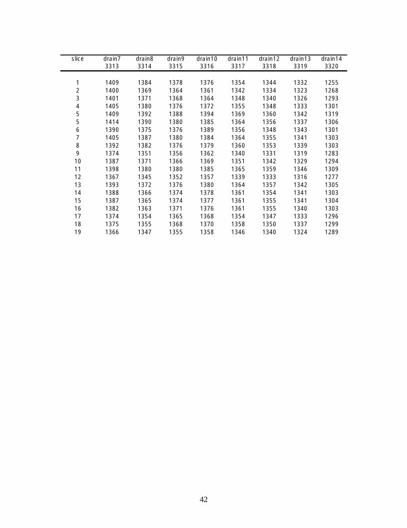
slice drain7 drain8 drain9 drain10 drain11 drain12 drain13 drain143313 3314 3315 3316 3317 3318 3319 3320

1 1409 1384 1378 1376 1354 1344 1332 12552 1400 1369 1364 1361 1342 1334 1323 12683 1401 1371 1368 1364 1348 1340 1326 12934 1405 1380 1376 1372 1355 1348 1333 13015 1409 1392 1388 1394 1369 1360 1342 13195 1414 1390 1380 1385 1364 1356 1337 13066 1390 1375 1376 1389 1356 1348 1343 13017 1405 1387 1380 1384 1364 1355 1341 13038 1392 1382 1376 1379 1360 1353 1339 13039 1374 1351 1356 1362 1340 1331 1319 128310 1387 1371 1366 1369 1351 1342 1329 129411 1398 1380 1380 1385 1365 1359 1346 130912 1367 1345 1352 1357 1339 1333 1316 127713 1393 1372 1376 1380 1364 1357 1342 130514 1388 1366 1374 1378 1361 1354 1341 130315 1387 1365 1374 1377 1361 1355 1341 130416 1382 1363 1371 1376 1361 1355 1340 130317 1374 1354 1365 1368 1354 1347 1333 129618 1375 1355 1368 1370 1358 1350 1337 129919 1366 1347 1355 1358 1346 1340 1324 1289

43

B.Data and Calculations

steam1

inlet X Iw (Amperes) Vw (Volts) Is (Amperes) Vs (Volts) mw (kg/s) ms (kg/s)

1.00E+00 0.000 0 1.225 96.2 0.00E+00 3.83E-05

distance (cm) T (°C) P(psig) P(bars) µs (cp) µw (cp)

ST inlet 0 130.322 13.908 1.972HW inlet 0 126.968 14.209 1.993

1 3.5 155.380 13.089 1.916 0.01292 0.23452 8.5 148.532 11.626 1.815 0.01286 0.23813 13.5 141.960 10.198 1.716 0.01280 0.24194 18.5 136.496 8.827 1.622 0.01274 0.24595 23.5 128.876 7.085 1.502 0.01266 0.25146 28.5 112.771 5.768 1.411 0.01259 0.25597 33.5 115.602 4.316 1.311 0.01252 0.26148 38.5 109.824 2.475 1.184 0.01242 0.2693

outlet 43.5 102.736 0.481 1.046 0.01230 0.2792

ρs (kg/m3) ρw (kg/m3) krs krw Sst krs (corr)

1 1.0844 944.03 1.6858 0.0000 1.000 1.36302 1.0309 945.37 0.9882 0.0000 1.000 0.79063 0.9784 946.73 1.0618 0.0000 1.000 0.83984 0.9279 948.09 1.1607 0.0000 1.000 0.90705 0.8635 949.89 0.9755 0.0000 1.000 0.74926 0.8145 951.31 1.3609 0.0000 1.000 1.02997 0.7604 952.95 1.3145 0.0000 1.000 0.97668 0.6913 955.16 1.1312 0.0000 1.000 0.8178

outlet 0.6159 957.72 1.1608 0.0000 1.000 0.8098mean 1.1727 0.0000 1.000 0.8929

44

flow2


8.89E-01 0.000 0 1.200 94.3 4.17E-06 3.33E-05


ST inlet 0 130.772 15.561 2.086HW inlet 0 127.320 15.286 2.067

1 3.5 120.616 14.466 2.011 0.01297 0.23132 8.5 119.209 13.082 1.915 0.01292 0.23453 13.5 117.491 11.583 1.812 0.01286 0.23824 18.5 115.879 10.100 1.710 0.01279 0.24225 23.5 113.927 8.568 1.604 0.01273 0.24676 28.5 111.169 6.966 1.494 0.01265 0.25187 33.5 109.152 5.052 1.362 0.01256 0.25868 38.5 106.921 3.250 1.237 0.01246 0.2659

outlet 43.5 102.472 0.430 1.043 0.01230 0.2795


1 1.1346 942.80 1.0521 0.0038 0.809 0.85852 1.0841 944.03 0.8676 0.0023 0.694 0.70153 1.0293 945.41 0.8399 0.0021 0.678 0.67174 0.9748 946.83 0.8920 0.0022 0.691 0.70505 0.9184 948.35 0.9118 0.0021 0.671 0.71086 0.8591 950.02 0.9267 0.0021 0.661 0.71087 0.7879 952.11 0.8395 0.0018 0.658 0.62978 0.7204 954.21 0.9677 0.0019 0.653 0.7081

outlet 0.6140 957.79 0.7158 0.0013 0.651 0.4989mean 0.8813 0.0020 0.670 0.6759

45

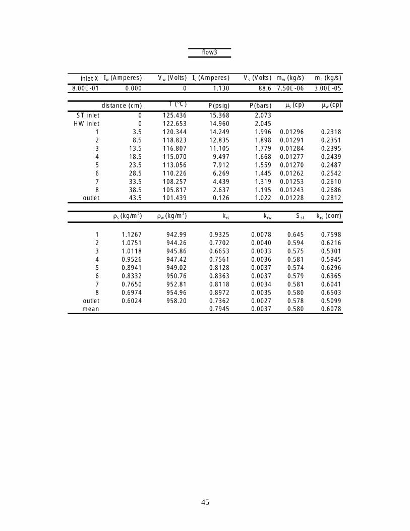
flow3


8.00E-01 0.000 0 1.130 88.6 7.50E-06 3.00E-05


ST inlet 0 125.436 15.368 2.073HW inlet 0 122.653 14.960 2.045

1 3.5 120.344 14.249 1.996 0.01296 0.23182 8.5 118.823 12.835 1.898 0.01291 0.23513 13.5 116.807 11.105 1.779 0.01284 0.23954 18.5 115.070 9.497 1.668 0.01277 0.24395 23.5 113.056 7.912 1.559 0.01270 0.24876 28.5 110.226 6.269 1.445 0.01262 0.25427 33.5 108.257 4.439 1.319 0.01253 0.26108 38.5 105.817 2.637 1.195 0.01243 0.2686

outlet 43.5 101.439 0.126 1.022 0.01228 0.2812


1 1.1267 942.99 0.9325 0.0078 0.645 0.75982 1.0751 944.26 0.7702 0.0040 0.594 0.62163 1.0118 945.86 0.6653 0.0033 0.575 0.53014 0.9526 947.42 0.7561 0.0036 0.581 0.59455 0.8941 949.02 0.8128 0.0037 0.574 0.62966 0.8332 950.76 0.8363 0.0037 0.579 0.63657 0.7650 952.81 0.8118 0.0034 0.581 0.60418 0.6974 954.96 0.8972 0.0035 0.580 0.6503

outlet 0.6024 958.20 0.7362 0.0027 0.578 0.5099mean 0.7945 0.0037 0.580 0.6078

46

flow4


7.00E-01 0.000 0 1.060 83.3 1.05E-05 2.45E-05


ST inlet 0 128.011 14.673 2.025HW inlet 0 125.368 14.208 1.993

1 3.5 119.604 13.613 1.952 0.01294 0.23332 8.5 118.018 12.208 1.855 0.01288 0.23663 13.5 116.106 10.528 1.739 0.01281 0.24104 18.5 114.465 9.001 1.634 0.01275 0.24545 23.5 112.457 7.495 1.530 0.01268 0.25006 28.5 109.698 5.924 1.422 0.01260 0.25547 33.5 107.844 4.219 1.304 0.01251 0.26188 38.5 105.609 2.522 1.187 0.01242 0.2691

outlet 43.5 101.867 0.202 1.027 0.01228 0.2808


1 1.1035 943.55 0.8193 0.0132 0.609 0.66482 1.0522 944.83 0.6455 0.0057 0.567 0.51873 0.9906 946.41 0.5704 0.0048 0.558 0.45244 0.9344 947.91 0.6619 0.0054 0.551 0.51815 0.8787 949.46 0.7098 0.0056 0.557 0.54756 0.8204 951.14 0.7245 0.0054 0.568 0.54927 0.7567 953.07 0.7186 0.0051 0.567 0.53328 0.6930 955.10 0.7825 0.0053 0.566 0.5662

outlet 0.6053 958.10 0.6479 0.0040 0.563 0.4494mean 0.6904 0.0055 0.562 0.5267

47

flow5b


6.00E-01 0.000 0 0.968 75.7 1.33E-05 2.00E-05


ST inlet 0 122.322 14.230 1.994HW inlet 0 119.683 14.014 1.979

1 3.5 119.383 13.342 1.933 0.01293 0.23392 8.5 117.944 11.971 1.839 0.01287 0.23723 13.5 115.951 10.276 1.722 0.01280 0.24174 18.5 114.076 8.694 1.613 0.01273 0.24635 23.5 112.127 7.189 1.509 0.01266 0.25106 28.5 109.418 5.601 1.399 0.01259 0.25657 33.5 107.519 3.947 1.285 0.01250 0.26298 38.5 105.383 2.335 1.174 0.01241 0.2700

outlet 43.5 101.518 0.362 1.038 0.01229 0.2799


1 1.0936 943.80 0.8049 0.0149 0.563 0.65202 1.0435 945.05 0.5441 0.0074 0.545 0.43653 0.9813 946.66 0.4655 0.0061 0.533 0.36844 0.9230 948.22 0.5274 0.0066 0.497 0.41165 0.8673 949.78 0.5867 0.0071 0.513 0.45116 0.8083 951.50 0.5930 0.0068 0.524 0.44797 0.7465 953.38 0.6123 0.0067 0.528 0.45268 0.6860 955.33 0.6788 0.0071 0.532 0.4896

outlet 0.6114 957.88 0.6162 0.0060 0.527 0.4289mean 0.5904 0.0071 0.525 0.4499

48

flow6


5.00E-01 0.000 0 0.980 76.4 2.08E-05 2.08E-05


ST inlet 0 123.915 14.565 2.017HW inlet 0 120.223 14.129 1.987

1 3.5 119.649 13.415 1.938 0.01293 0.23372 8.5 118.139 12.080 1.846 0.01288 0.23703 13.5 116.232 10.373 1.728 0.01281 0.24154 18.5 114.370 8.774 1.618 0.01274 0.24605 23.5 112.379 7.266 1.514 0.01267 0.25086 28.5 109.551 5.651 1.403 0.01259 0.25647 33.5 107.713 4.018 1.290 0.01250 0.26268 38.5 105.581 2.406 1.179 0.01241 0.2696

outlet 43.5 101.753 0.448 1.044 0.01230 0.2794


1 1.0963 943.73 0.6460 0.0219 0.535 0.52352 1.0475 944.95 0.5801 0.0118 0.522 0.46573 0.9849 946.56 0.4799 0.0094 0.510 0.38014 0.9260 948.14 0.5419 0.0102 0.488 0.42335 0.8702 949.70 0.6081 0.0110 0.486 0.46806 0.8102 951.44 0.6061 0.0105 0.501 0.45807 0.7492 953.30 0.6439 0.0106 0.506 0.47648 0.6887 955.24 0.7045 0.0110 0.507 0.5088

outlet 0.6146 957.77 0.6437 0.0094 0.506 0.4488mean 0.5991 0.0111 0.503 0.4577

49

flow7


4.10E-01 0.000 0 1.012 79.3 3.00E-05 2.08E-05


ST inlet 0 126.375 15.667 2.093HW inlet 0 121.298 15.254 2.065

1 3.5 120.522 14.526 2.015 0.01297 0.23122 8.5 119.086 13.150 1.920 0.01292 0.23443 13.5 116.927 11.299 1.792 0.01284 0.23904 18.5 115.003 9.565 1.673 0.01277 0.24375 23.5 112.903 7.896 1.558 0.01270 0.24876 28.5 109.940 6.172 1.439 0.01261 0.25457 33.5 108.039 4.300 1.310 0.01252 0.26158 38.5 105.585 2.519 1.187 0.01242 0.2691

outlet 43.5 101.500 0.466 1.045 0.01230 0.2793


1 1.1368 942.75 0.6300 0.0306 0.523 0.51422 1.0866 943.97 0.5443 0.0164 0.507 0.44033 1.0189 945.68 0.4291 0.0124 0.495 0.34244 0.9551 947.35 0.4858 0.0135 0.480 0.38225 0.8935 949.04 0.5364 0.0142 0.474 0.41546 0.8296 950.87 0.5557 0.0141 0.485 0.42257 0.7598 952.97 0.5545 0.0133 0.488 0.41198 0.6929 955.10 0.6341 0.0144 0.478 0.4588

outlet 0.6153 957.74 0.6133 0.0129 0.484 0.4277mean 0.5458 0.0147 0.487 0.4191

50

flow8


3.02E-01 0.000 0 0.963 75.2 4.17E-05 1.80E-05


ST inlet 0 124.279 15.019 2.049HW inlet 0 120.387 14.628 2.022

1 3.5 120.986 13.961 1.976 0.01295 0.23252 8.5 119.517 12.692 1.888 0.01290 0.23553 13.5 117.579 10.982 1.770 0.01283 0.23984 18.5 115.763 9.342 1.657 0.01276 0.24445 23.5 113.657 7.727 1.546 0.01269 0.24936 28.5 110.702 6.066 1.431 0.01261 0.25497 33.5 108.700 4.184 1.302 0.01251 0.26208 38.5 106.141 2.322 1.173 0.01241 0.2700

outlet 43.5 101.843 0.148 1.023 0.01228 0.2811


1 1.1162 943.24 0.5968 0.0466 0.477 0.48542 1.0699 944.39 0.5172 0.0248 0.474 0.41703 1.0072 945.98 0.4055 0.0187 0.467 0.32284 0.9469 947.57 0.4473 0.0198 0.444 0.35125 0.8873 949.22 0.4820 0.0205 0.449 0.37276 0.8256 950.99 0.5005 0.0203 0.460 0.38017 0.7554 953.11 0.4791 0.0184 0.434 0.35538 0.6855 955.35 0.5292 0.0191 0.463 0.3817

outlet 0.6033 958.17 0.5095 0.0170 0.463 0.3531mean 0.4912 0.0210 0.457 0.3752

51

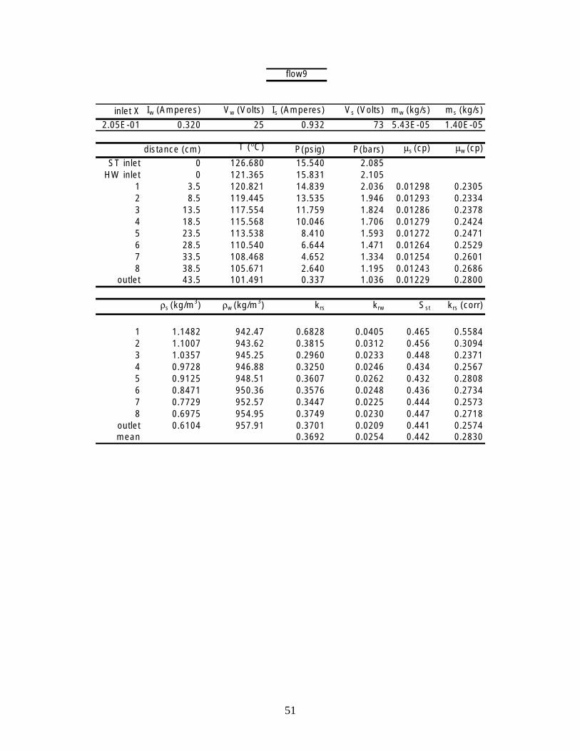
flow9


2.05E-01 0.320 25 0.932 73 5.43E-05 1.40E-05


ST inlet 0 126.680 15.540 2.085HW inlet 0 121.365 15.831 2.105

1 3.5 120.821 14.839 2.036 0.01298 0.23052 8.5 119.445 13.535 1.946 0.01293 0.23343 13.5 117.554 11.759 1.824 0.01286 0.23784 18.5 115.568 10.046 1.706 0.01279 0.24245 23.5 113.538 8.410 1.593 0.01272 0.24716 28.5 110.540 6.644 1.471 0.01264 0.25297 33.5 108.468 4.652 1.334 0.01254 0.26018 38.5 105.671 2.640 1.195 0.01243 0.2686

outlet 43.5 101.491 0.337 1.036 0.01229 0.2800


1 1.1482 942.47 0.6828 0.0405 0.465 0.55842 1.1007 943.62 0.3815 0.0312 0.456 0.30943 1.0357 945.25 0.2960 0.0233 0.448 0.23714 0.9728 946.88 0.3250 0.0246 0.434 0.25675 0.9125 948.51 0.3607 0.0262 0.432 0.28086 0.8471 950.36 0.3576 0.0248 0.436 0.27347 0.7729 952.57 0.3447 0.0225 0.444 0.25738 0.6975 954.95 0.3749 0.0230 0.447 0.2718

outlet 0.6104 957.91 0.3701 0.0209 0.441 0.2574mean 0.3692 0.0254 0.442 0.2830

52

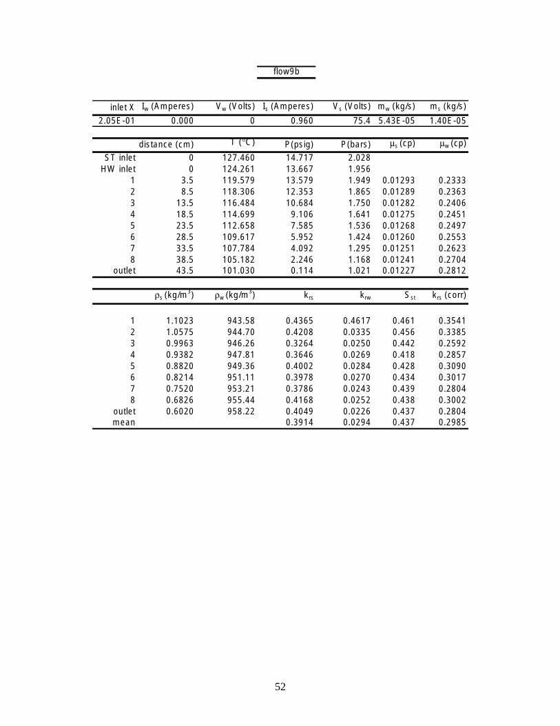
flow9b


2.05E-01 0.000 0 0.960 75.4 5.43E-05 1.40E-05


ST inlet 0 127.460 14.717 2.028HW inlet 0 124.261 13.667 1.956

1 3.5 119.579 13.579 1.949 0.01293 0.23332 8.5 118.306 12.353 1.865 0.01289 0.23633 13.5 116.484 10.684 1.750 0.01282 0.24064 18.5 114.699 9.106 1.641 0.01275 0.24515 23.5 112.658 7.585 1.536 0.01268 0.24976 28.5 109.617 5.952 1.424 0.01260 0.25537 33.5 107.784 4.092 1.295 0.01251 0.26238 38.5 105.182 2.246 1.168 0.01241 0.2704

outlet 43.5 101.030 0.114 1.021 0.01227 0.2812


1 1.1023 943.58 0.4365 0.4617 0.461 0.35412 1.0575 944.70 0.4208 0.0335 0.456 0.33853 0.9963 946.26 0.3264 0.0250 0.442 0.25924 0.9382 947.81 0.3646 0.0269 0.418 0.28575 0.8820 949.36 0.4002 0.0284 0.428 0.30906 0.8214 951.11 0.3978 0.0270 0.434 0.30177 0.7520 953.21 0.3786 0.0243 0.439 0.28048 0.6826 955.44 0.4168 0.0252 0.438 0.3002

outlet 0.6020 958.22 0.4049 0.0226 0.437 0.2804mean 0.3914 0.0294 0.437 0.2985

53

flow10


9.09E-02 0.473 37 0.853 66.8 9.17E-05 9.17E-06


ST inlet 0 128.509 16.068 2.121HW inlet 0 120.015 16.322 2.139

1 3.5 121.474 15.914 2.110 0.01302 0.22822 8.5 120.538 14.669 2.025 0.01298 0.23093 13.5 118.933 12.949 1.906 0.01291 0.23484 18.5 117.075 11.196 1.785 0.01284 0.23925 23.5 114.862 9.411 1.662 0.01276 0.24426 28.5 111.604 7.296 1.516 0.01267 0.25077 33.5 108.940 5.005 1.358 0.01256 0.25888 38.5 2.652 1.196 0.01243 0.2685

outlet 43.5 0.273 1.032 0.01229 0.2804


1 1.1873 941.55 1.9741 0.1646 0.406 1.62482 1.1420 942.62 0.2530 0.0545 0.422 0.20673 1.0793 944.15 0.1928 0.0401 0.417 0.15574 1.0151 945.78 0.2000 0.0400 0.395 0.15955 0.9495 947.51 0.2088 0.0400 0.407 0.16406 0.8713 949.67 0.1906 0.0346 0.410 0.14677 0.7861 952.17 0.1933 0.0329 0.417 0.14498 0.6979 954.94 0.2098 0.0331 0.424 0.1521

outlet 0.6080 958.00 0.2354 0.0341 0.420 0.1636mean 0.2315 0.0413 0.414 0.1777

54

flow11


1.19E-02 0.864 68.1 0.688 54.3 1.67E-04 2.00E-06


ST inlet 0 129.384 16.811 2.172HW inlet 0 123.661 17.389 2.212

1 3.5 122.358 16.053 2.120 0.01303 0.22792 8.5 120.694 14.481 2.012 0.01297 0.23133 13.5 118.463 12.278 1.860 0.01288 0.23654 18.5 116.344 10.398 1.730 0.01281 0.24145 23.5 113.954 8.602 1.606 0.01273 0.24666 28.5 110.538 6.614 1.469 0.01264 0.25307 33.5 108.536 4.524 1.325 0.01253 0.26068 38.5 2.532 1.188 0.01242 0.2690

outlet 43.5 0.093 1.020 0.01227 0.2814


1 1.1923 941.43 0.0872 0.0913 0.391 0.07182 1.1352 942.79 0.0440 0.0786 0.383 0.03593 1.0547 944.77 0.0335 0.0573 0.372 0.02704 0.9858 946.54 0.0418 0.0684 0.349 0.03315 0.9196 948.32 0.0466 0.0730 0.362 0.03636 0.8460 950.39 0.0454 0.0675 0.354 0.03477 0.7681 952.71 0.0472 0.0660 0.360 0.03528 0.6934 955.08 0.0544 0.0713 0.363 0.0394

outlet 0.6012 958.25 0.0506 0.0607 0.363 0.0350mean 0.0472 0.0693 0.363 0.0363

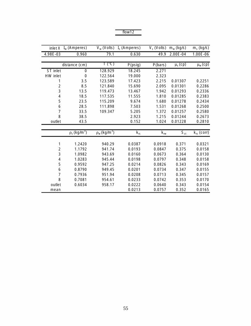
55

flow12


4.98E-03 0.960 79.1 0.630 49.9 2.00E-04 1.00E-06


ST inlet 0 128.929 18.245 2.271HW inlet 0 122.564 19.000 2.323

1 3.5 123.589 17.423 2.215 0.01307 0.22512 8.5 121.840 15.690 2.095 0.01301 0.22863 13.5 119.473 13.467 1.942 0.01293 0.23364 18.5 117.535 11.555 1.810 0.01285 0.23835 23.5 115.209 9.674 1.680 0.01278 0.24346 28.5 111.898 7.503 1.531 0.01268 0.25007 33.5 109.347 5.205 1.372 0.01257 0.25808 38.5 2.923 1.215 0.01244 0.2673

outlet 43.5 0.152 1.024 0.01228 0.2810


1 1.2420 940.29 0.0387 0.0918 0.371 0.03212 1.1792 941.74 0.0193 0.0847 0.375 0.01583 1.0982 943.69 0.0160 0.0673 0.364 0.01304 1.0283 945.44 0.0198 0.0797 0.348 0.01585 0.9592 947.25 0.0214 0.0826 0.343 0.01696 0.8790 949.45 0.0201 0.0734 0.347 0.01557 0.7936 951.94 0.0208 0.0713 0.345 0.01578 0.7081 954.61 0.0233 0.0742 0.353 0.0170

outlet 0.6034 958.17 0.0222 0.0640 0.343 0.0154mean 0.0213 0.0757 0.352 0.0165

56

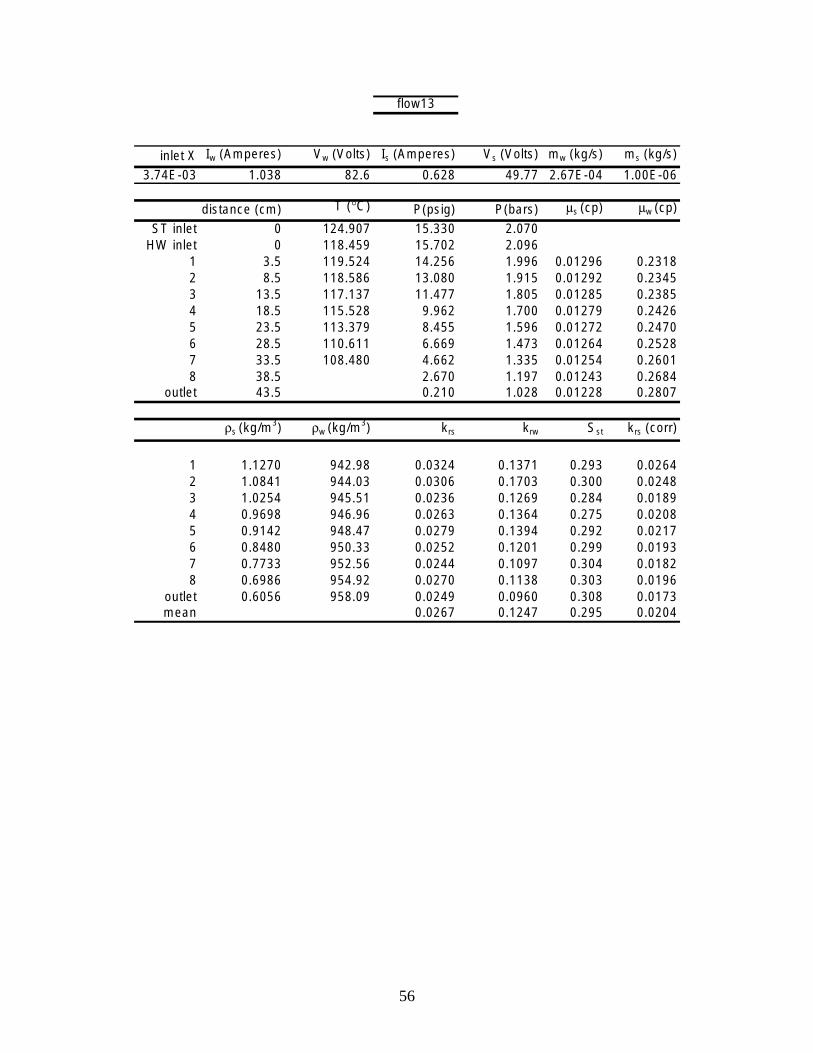
flow13


3.74E-03 1.038 82.6 0.628 49.77 2.67E-04 1.00E-06


ST inlet 0 124.907 15.330 2.070HW inlet 0 118.459 15.702 2.096

1 3.5 119.524 14.256 1.996 0.01296 0.23182 8.5 118.586 13.080 1.915 0.01292 0.23453 13.5 117.137 11.477 1.805 0.01285 0.23854 18.5 115.528 9.962 1.700 0.01279 0.24265 23.5 113.379 8.455 1.596 0.01272 0.24706 28.5 110.611 6.669 1.473 0.01264 0.25287 33.5 108.480 4.662 1.335 0.01254 0.26018 38.5 2.670 1.197 0.01243 0.2684

outlet 43.5 0.210 1.028 0.01228 0.2807


1 1.1270 942.98 0.0324 0.1371 0.293 0.02642 1.0841 944.03 0.0306 0.1703 0.300 0.02483 1.0254 945.51 0.0236 0.1269 0.284 0.01894 0.9698 946.96 0.0263 0.1364 0.275 0.02085 0.9142 948.47 0.0279 0.1394 0.292 0.02176 0.8480 950.33 0.0252 0.1201 0.299 0.01937 0.7733 952.56 0.0244 0.1097 0.304 0.01828 0.6986 954.92 0.0270 0.1138 0.303 0.0196

outlet 0.6056 958.09 0.0249 0.0960 0.308 0.0173mean 0.0267 0.1247 0.295 0.0204

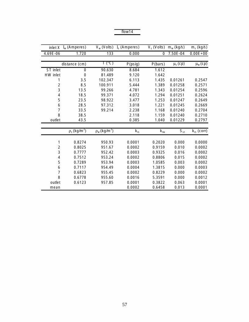
57

flow14


4.69E-06 1.720 133 0.000 0 7.50E-04 0.00E+00


ST inlet 0 90.630 8.684 1.612HW inlet 0 81.489 9.120 1.642

1 3.5 102.347 6.113 1.435 0.01261 0.25472 8.5 100.911 5.444 1.389 0.01258 0.25713 13.5 99.266 4.781 1.343 0.01254 0.25964 18.5 99.371 4.072 1.294 0.01251 0.26245 23.5 98.922 3.477 1.253 0.01247 0.26496 28.5 97.312 3.018 1.221 0.01245 0.26697 33.5 99.214 2.238 1.168 0.01240 0.27048 38.5 2.118 1.159 0.01240 0.2710

outlet 43.5 0.385 1.040 0.01229 0.2797


1 0.8274 950.93 0.0001 0.2020 0.000 0.00002 0.8025 951.67 0.0002 0.9159 0.010 0.00023 0.7777 952.42 0.0003 0.9325 0.016 0.00024 0.7512 953.24 0.0002 0.8806 0.015 0.00025 0.7289 953.94 0.0003 1.0585 0.003 0.00026 0.7117 954.49 0.0004 1.3815 0.000 0.00037 0.6823 955.45 0.0002 0.8229 0.000 0.00028 0.6778 955.60 0.0016 5.3591 0.000 0.0012

outlet 0.6123 957.85 0.0001 0.3822 0.063 0.0001mean 0.0002 0.6458 0.013 0.0001

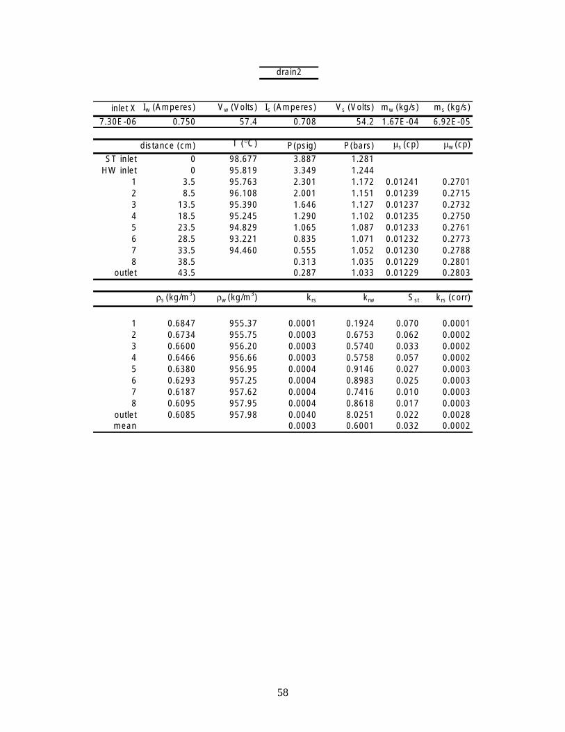
58

drain2


7.30E-06 0.750 57.4 0.708 54.2 1.67E-04 6.92E-05


ST inlet 0 98.677 3.887 1.281HW inlet 0 95.819 3.349 1.244

1 3.5 95.763 2.301 1.172 0.01241 0.27012 8.5 96.108 2.001 1.151 0.01239 0.27153 13.5 95.390 1.646 1.127 0.01237 0.27324 18.5 95.245 1.290 1.102 0.01235 0.27505 23.5 94.829 1.065 1.087 0.01233 0.27616 28.5 93.221 0.835 1.071 0.01232 0.27737 33.5 94.460 0.555 1.052 0.01230 0.27888 38.5 0.313 1.035 0.01229 0.2801

outlet 43.5 0.287 1.033 0.01229 0.2803


1 0.6847 955.37 0.0001 0.1924 0.070 0.00012 0.6734 955.75 0.0003 0.6753 0.062 0.00023 0.6600 956.20 0.0003 0.5740 0.033 0.00024 0.6466 956.66 0.0003 0.5758 0.057 0.00025 0.6380 956.95 0.0004 0.9146 0.027 0.00036 0.6293 957.25 0.0004 0.8983 0.025 0.00037 0.6187 957.62 0.0004 0.7416 0.010 0.00038 0.6095 957.95 0.0004 0.8618 0.017 0.0003

outlet 0.6085 957.98 0.0040 8.0251 0.022 0.0028mean 0.0003 0.6001 0.032 0.0002

59

drain3


2.31E-05 1.068 81.9 0.000 0 2.67E-04 0.00E+00


ST inlet 0 94.907 4.088 1.295HW inlet 0 88.979 4.169 1.301

1 3.5 99.147 3.746 1.272 0.01249 0.26382 8.5 97.873 2.678 1.198 0.01243 0.26843 13.5 96.554 2.367 1.176 0.01241 0.26984 18.5 96.418 1.973 1.149 0.01239 0.27175 23.5 95.893 1.688 1.130 0.01237 0.27306 28.5 93.989 1.389 1.109 0.01235 0.27457 33.5 95.498 0.953 1.079 0.01233 0.27678 38.5 0.352 1.038 0.01229 0.2799

outlet 43.5 0.315 1.035 0.01229 0.2801


1 0.7390 953.62 0.0007 0.5273 0.035 0.00052 0.6989 954.91 0.0003 0.2122 0.031 0.00023 0.6872 955.29 0.0011 0.7323 0.043 0.00084 0.6724 955.78 0.0009 0.5817 0.059 0.00065 0.6616 956.14 0.0012 0.8079 0.072 0.00096 0.6503 956.53 0.0012 0.7740 0.048 0.00087 0.6338 957.09 0.0008 0.5347 0.081 0.00068 0.6110 957.89 0.0006 0.3921 0.129 0.0004

outlet 0.6096 957.94 0.0101 6.3732 0.173 0.0071mean 0.0008 0.5357 0.079 0.0006

60

drain4


4.20E-05 1.140 82.2 0.000 0 2.42E-04 0.00E+00


ST inlet 0 101.682 4.679 1.336HW inlet 0 95.564 4.977 1.356

1 3.5 105.317 3.771 1.273 0.01249 0.26372 8.5 104.220 3.631 1.264 0.01248 0.26423 13.5 103.597 3.009 1.221 0.01245 0.26694 18.5 103.445 2.865 1.211 0.01244 0.26765 23.5 102.930 2.543 1.189 0.01242 0.26906 28.5 102.089 1.787 1.136 0.01238 0.27257 33.5 102.016 1.496 1.116 0.01236 0.27408 38.5 1.456 1.114 0.01236 0.2742

outlet 43.5 0.422 1.042 0.01229 0.2795


1 0.7400 953.59 0.0004 0.1675 0.094 0.00032 0.7347 953.76 0.0037 1.4462 0.085 0.00273 0.7114 954.50 0.0009 0.3285 0.069 0.00064 0.7059 954.68 0.0038 1.4222 0.090 0.00275 0.6938 955.07 0.0017 0.6392 0.108 0.00126 0.6653 956.02 0.0008 0.2756 0.084 0.00057 0.6543 956.39 0.0020 0.7194 0.097 0.00148 0.6528 956.44 0.0145 5.2369 0.136 0.0103

outlet 0.6137 957.80 0.0006 0.2063 0.165 0.0004mean 0.0011 0.4085 0.104 0.0008

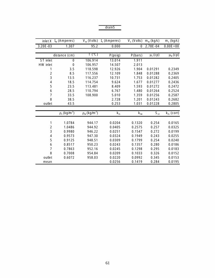
61

drain5


3.20E-03 1.307 95.2 0.000 0 2.78E-04 0.00E+00


ST inlet 0 106.914 13.014 1.911HW inlet 0 106.957 14.507 2.013

1 3.5 118.598 12.926 1.904 0.01291 0.23492 8.5 117.556 12.109 1.848 0.01288 0.23693 13.5 116.237 10.731 1.753 0.01282 0.24054 18.5 114.754 9.624 1.677 0.01277 0.24365 23.5 113.481 8.409 1.593 0.01272 0.24726 28.5 110.794 6.767 1.480 0.01264 0.25247 33.5 108.900 5.010 1.359 0.01256 0.25878 38.5 2.728 1.201 0.01243 0.2682

outlet 43.5 0.253 1.031 0.01228 0.2805


1 1.0784 944.17 0.0204 0.1320 0.254 0.01652 1.0486 944.92 0.0405 0.2575 0.257 0.03253 0.9980 946.22 0.0251 0.1547 0.272 0.01994 0.9573 947.30 0.0324 0.1949 0.243 0.02555 0.9125 948.51 0.0309 0.1799 0.254 0.02406 0.8517 950.23 0.0243 0.1357 0.280 0.01867 0.7863 952.16 0.0245 0.1298 0.295 0.01838 0.7008 954.84 0.0209 0.1033 0.326 0.0152

outlet 0.6072 958.03 0.0220 0.0992 0.345 0.0153mean 0.0256 0.1419 0.284 0.0195

62

drain6


5.84E-04 1.530 111.5 0.000 0 4.17E-04


ST inlet 0 110.698 14.577 2.018HW inlet 0 107.011 16.260 2.134

1 3.5 119.885 14.254 1.996 0.01296 0.23182 8.5 118.443 13.716 1.959 0.01294 0.23303 13.5 117.516 12.836 1.898 0.01291 0.23514 18.5 116.562 12.220 1.856 0.01288 0.23665 23.5 115.853 11.846 1.830 0.01287 0.23766 28.5 115.024 9.906 1.696 0.01279 0.24287 33.5 112.237 7.573 1.535 0.01268 0.24988 38.5 3.786 1.274 0.01249 0.2636

outlet 43.5 101.353 0.282 1.033 0.01229 0.2803


1 1.1269 942.99 0.0042 0.1543 0.180 0.00342 1.1073 943.46 0.0160 0.5781 0.126 0.01303 1.0752 944.25 0.0100 0.3563 0.082 0.00814 1.0526 944.82 0.0146 0.5120 0.133 0.01185 1.0389 945.17 0.0244 0.8463 0.156 0.01956 0.9677 947.02 0.0050 0.1664 0.197 0.00407 0.8816 949.38 0.0045 0.1420 0.315 0.00358 0.7405 953.57 0.0033 0.0919 0.347 0.0024

outlet 0.6083 957.99 0.0042 0.1052 0.353 0.0029mean 0.0061 0.1891 0.214 0.0047

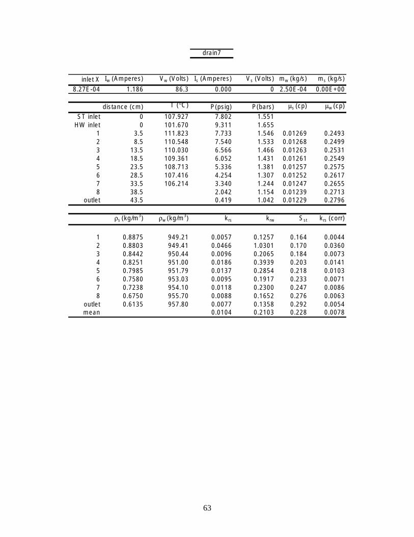
63

drain7


8.27E-04 1.186 86.3 0.000 0 2.50E-04 0.00E+00


ST inlet 0 107.927 7.802 1.551HW inlet 0 101.670 9.311 1.655

1 3.5 111.823 7.733 1.546 0.01269 0.24932 8.5 110.548 7.540 1.533 0.01268 0.24993 13.5 110.030 6.566 1.466 0.01263 0.25314 18.5 109.361 6.052 1.431 0.01261 0.25495 23.5 108.713 5.336 1.381 0.01257 0.25756 28.5 107.416 4.254 1.307 0.01252 0.26177 33.5 106.214 3.340 1.244 0.01247 0.26558 38.5 2.042 1.154 0.01239 0.2713

outlet 43.5 0.419 1.042 0.01229 0.2796


1 0.8875 949.21 0.0057 0.1257 0.164 0.00442 0.8803 949.41 0.0466 1.0301 0.170 0.03603 0.8442 950.44 0.0096 0.2065 0.184 0.00734 0.8251 951.00 0.0186 0.3939 0.203 0.01415 0.7985 951.79 0.0137 0.2854 0.218 0.01036 0.7580 953.03 0.0095 0.1917 0.233 0.00717 0.7238 954.10 0.0118 0.2300 0.247 0.00868 0.6750 955.70 0.0088 0.1652 0.276 0.0063

outlet 0.6135 957.80 0.0077 0.1358 0.292 0.0054mean 0.0104 0.2103 0.228 0.0078

64

drain8


5.56E-03 1.275 92.8 0.000 0 2.67E-04 0.00E+00


ST inlet 0 114.345 14.126 1.987HW inlet 0 107.168 15.797 2.102

1 3.5 119.878 13.992 1.978 0.01295 0.23242 8.5 118.826 13.155 1.920 0.01292 0.23433 13.5 117.695 11.909 1.834 0.01287 0.23744 18.5 116.245 10.687 1.750 0.01282 0.24065 23.5 114.898 9.572 1.673 0.01277 0.24376 28.5 112.397 7.839 1.554 0.01269 0.24897 33.5 109.976 5.718 1.407 0.01259 0.25618 38.5 3.013 1.221 0.01245 0.2669

outlet 43.5 0.300 1.034 0.01229 0.2802


1 1.1174 943.22 0.0288 0.1095 0.262 0.02342 1.0868 943.97 0.0637 0.2378 0.288 0.05153 1.0412 945.11 0.0445 0.1617 0.270 0.03574 0.9964 946.26 0.0472 0.1669 0.262 0.03755 0.9554 947.35 0.0538 0.1850 0.278 0.04236 0.8914 949.10 0.0368 0.1214 0.307 0.02857 0.8127 951.37 0.0328 0.1018 0.331 0.02488 0.7115 954.50 0.0290 0.0829 0.351 0.0212

outlet 0.6090 957.96 0.0333 0.0865 0.369 0.0232mean 0.0383 0.1239 0.307 0.0294

65

drain9


4.67E-03 1.275 92.3 0.000 0 2.50E-04 0.00E+00


ST inlet 0 113.334 12.917 1.904HW inlet 0 107.015 14.998 2.047

1 3.5 118.722 12.893 1.902 0.01291 0.23502 8.5 117.723 12.104 1.848 0.01288 0.23693 13.5 116.057 10.505 1.738 0.01281 0.24114 18.5 114.637 9.237 1.650 0.01276 0.24475 23.5 112.749 7.863 1.555 0.01269 0.24896 28.5 110.287 5.955 1.424 0.01260 0.25537 33.5 108.056 4.488 1.323 0.01253 0.26088 38.5 2.663 1.197 0.01243 0.2685

outlet 43.5 0.370 1.039 0.01229 0.2798


1 1.0772 944.20 0.0201 0.0890 0.285 0.01622 1.0484 944.93 0.0549 0.2391 0.304 0.04413 0.9897 946.44 0.0286 0.1199 0.293 0.02264 0.9431 947.68 0.0376 0.1532 0.274 0.02955 0.8923 949.07 0.0365 0.1436 0.286 0.02836 0.8215 951.11 0.0284 0.1058 0.295 0.02157 0.7668 952.75 0.0393 0.1404 0.304 0.02938 0.6983 954.92 0.0344 0.1159 0.315 0.0249

outlet 0.6117 957.87 0.0309 0.0959 0.327 0.0215mean 0.0322 0.1235 0.300 0.0247

66

drain10


3.47E-03 1.137 82.9 0.000 0 2.00E-04 0.00E+00


ST inlet 0 107.724 9.874 1.694HW inlet 0 106.222 11.742 1.823

1 3.5 115.448 9.997 1.703 0.01279 0.24252 8.5 114.155 9.081 1.639 0.01275 0.24513 13.5 112.739 7.814 1.552 0.01269 0.24904 18.5 111.283 6.821 1.484 0.01265 0.25235 23.5 109.801 5.836 1.416 0.01260 0.25576 28.5 107.750 4.295 1.309 0.01252 0.26157 33.5 106.265 3.359 1.245 0.01247 0.26548 38.5 2.138 1.161 0.01240 0.2709

outlet 43.5 101.473 0.452 1.044 0.01230 0.2794


1 0.9710 946.93 0.0159 0.0884 0.293 0.01252 0.9373 947.83 0.0312 0.1702 0.317 0.02443 0.8905 949.13 0.0236 0.1248 0.284 0.01834 0.8537 950.17 0.0314 0.1611 0.244 0.02405 0.8171 951.24 0.0329 0.1645 0.272 0.02496 0.7596 952.98 0.0225 0.1073 0.276 0.01677 0.7245 954.08 0.0386 0.1791 0.289 0.02838 0.6786 955.57 0.0315 0.1399 0.299 0.0226

outlet 0.6148 957.76 0.0249 0.1043 0.318 0.0174mean 0.0263 0.1302 0.288 0.0198

67

drain11


1.84E-02 1.088 79.3 0.000 0 1.50E-04 0.00E+00

distance (cm) T (°C) P(psig) P(bars) µs µw

ST inlet 0 104.974 14.758 2.031HW inlet 0 111.299 15.492 2.081

1 3.5 119.050 13.096 1.916 0.01292 0.23452 8.5 117.370 11.789 1.826 0.01286 0.23773 13.5 115.553 10.039 1.705 0.01279 0.24244 18.5 113.809 8.597 1.606 0.01273 0.24665 23.5 111.744 7.142 1.506 0.01266 0.25126 28.5 109.200 5.264 1.376 0.01257 0.25787 33.5 107.172 3.891 1.282 0.01250 0.26328 38.5 2.330 1.174 0.01241 0.2700

outlet 43.5 0.387 1.040 0.01229 0.2797


1 1.0847 944.02 0.0415 0.0462 0.379 0.03352 1.0368 945.22 0.0792 0.0857 0.385 0.06353 0.9726 946.89 0.0627 0.0651 0.366 0.04964 0.9194 948.32 0.0801 0.0803 0.338 0.06255 0.8656 949.83 0.0839 0.0809 0.345 0.06456 0.7958 951.87 0.0702 0.0642 0.347 0.05287 0.7444 953.45 0.1021 0.0895 0.353 0.07548 0.6858 955.34 0.0968 0.0806 0.355 0.0698

outlet 0.6123 957.85 0.0863 0.0669 0.365 0.0601mean 0.0732 0.0705 0.357 0.0561

68

drain12


3.62E-02 1.040 75.5 0.000 0 1.17E-04 0.00E+00


ST inlet 0 111.913 14.896 2.040HW inlet 0 113.790 16.317 2.138

1 3.5 119.855 14.084 1.984 0.01295 0.23222 8.5 118.435 12.640 1.885 0.01290 0.23563 13.5 116.312 10.648 1.747 0.01282 0.24074 18.5 114.531 9.040 1.637 0.01275 0.24535 23.5 112.272 7.425 1.525 0.01267 0.25036 28.5 109.563 5.414 1.387 0.01258 0.25727 33.5 107.360 3.958 1.286 0.01250 0.26298 38.5 2.355 1.176 0.01241 0.2699

outlet 43.5 101.275 0.339 1.037 0.01229 0.2800


1 1.1207 943.14 0.0661 0.0375 0.418 0.05382 1.0680 944.43 0.1068 0.0587 0.416 0.08603 0.9950 946.30 0.0825 0.0434 0.398 0.06554 0.9358 947.88 0.1081 0.0547 0.368 0.08475 0.8761 949.53 0.1143 0.0555 0.376 0.08816 0.8014 951.71 0.0996 0.0457 0.369 0.07517 0.7470 953.37 0.1467 0.0644 0.379 0.10858 0.6868 955.30 0.1439 0.0599 0.380 0.1039

outlet 0.6105 957.91 0.1275 0.0493 0.392 0.0887mean 0.1043 0.0507 0.385 0.0803

69

drain13


1.99E-01 0.964 70.1 0.000 0 8.33E-05 0.00E+00


ST inlet 0 105.792 15.470 2.080HW inlet 0 113.521 16.843 2.175

1 3.5 120.488 14.557 2.017 0.01297 0.23112 8.5 118.727 13.023 1.911 0.01291 0.23473 13.5 116.434 10.801 1.758 0.01282 0.24034 18.5 114.475 9.056 1.638 0.01275 0.24525 23.5 112.177 7.379 1.522 0.01267 0.25046 28.5 109.571 5.378 1.384 0.01257 0.25747 33.5 107.351 3.918 1.283 0.01250 0.26318 38.5 2.277 1.170 0.01241 0.2702

outlet 43.5 100.944 0.364 1.038 0.01229 0.2799


1 1.1379 942.72 0.2496 0.0217 0.465 0.20382 1.0820 944.09 0.3895 0.0327 0.464 0.31483 1.0006 946.15 0.2888 0.0231 0.465 0.22954 0.9364 947.86 0.3906 0.0299 0.403 0.30595 0.8744 949.58 0.4327 0.0318 0.425 0.33336 0.8000 951.75 0.3933 0.0273 0.425 0.29627 0.7455 953.42 0.5749 0.0382 0.433 0.42488 0.6838 955.40 0.5536 0.0348 0.436 0.3989

outlet 0.6115 957.88 0.5261 0.0308 0.449 0.3661mean 0.3931 0.0291 0.438 0.3033

70

drain14


7.72E-01 1.209 88 0.000 0 3.33E-05 0.00E+00


ST inlet 0 141.114 12.420 1.870HW inlet 0 119.477 12.921 1.904

1 3.5 118.120 12.216 1.856 0.01288 0.23662 8.5 117.022 11.220 1.787 0.01284 0.23923 13.5 115.516 9.913 1.697 0.01279 0.24274 18.5 113.860 8.513 1.600 0.01272 0.24685 23.5 111.992 7.138 1.505 0.01266 0.25126 28.5 109.312 5.494 1.392 0.01258 0.25697 33.5 107.934 4.194 1.302 0.01251 0.26198 38.5 2.733 1.202 0.01243 0.2681

outlet 43.5 102.076 0.690 1.061 0.01231 0.2781


1 1.0525 944.82 1.3510 0.0082 0.766 1.08562 1.0160 945.75 0.9875 0.0058 0.634 0.78763 0.9680 947.01 0.7865 0.0045 0.578 0.62064 0.9163 948.41 0.7719 0.0043 0.546 0.60145 0.8654 949.83 0.8280 0.0044 0.558 0.63636 0.8043 951.62 0.7404 0.0038 0.566 0.55847 0.7558 953.09 0.9911 0.0049 0.578 0.73518 0.7010 954.84 0.9448 0.0044 0.578 0.6859

outlet 0.6238 957.44 0.7517 0.0033 0.592 0.5266mean 0.8758 0.0045 0.579 0.6645

Documents

CONSTANT-PRESSURE MEASUREMENT OF STEAM-WATER RELATIVE ... · Measurement of Steam-Water Relative Permeability ... Figure 5.6: Relative permeability, ... CONSTANT-PRESSURE MEASUREMENT