Representing Reconstructed Networks Mathematically: The ...systemsbiology.ucsd.edu/sites/default/files/Attachments/Images/... · Representing Reconstructed Networks Mathematically:

1

University of California, San DiegoDepartment of Bioengineering

Systems Biology Research Grouphttp://systemsbiology.ucsd.edu

Representing Reconstructed Networks Mathematically:The Stoichiometric Matrix

Bernhard PalssonLecture #4

September 15, 2003

2



Outline

1) The stoichiometric matrix- Constructing the S-matrix- Flux vectors- Connectivity

2) Topological properties and SVD of S- 4 fundamental subspaces of S- Singular value decomposition of S

3) The two null spaces of S: Pools and pathways- Open systems- Closed systems N(S)

v

vdyn

vss

Rn Rm

0 0

dtd

dyn

xC =

Cconsv

C

Smxn

R(S ) R(S)

N(S )

S tot

S int SexchS =

0

3



Stoichiometric Coefficients

A -a

B 0

C -c

D 0

E +e

F 0

G 0

H +h

• Integral numbers

• Universal biochemical constants• Constants: time-invariant

chemical reaction: aaA + A + ccC C vvii eeE + E + hhHH

com

poun

ds

viRepresentation as a column in a matrix:

EACH COLUMN IN THE STOICHIOMETRIC MATRIX CORRESPONDS TO A PARTICUALR METABOLIC BIOCHEMICAL

REACTION

The stoichiometric coefficients: They are integers (a,c,e,h in the example given) that represent the number of molecules of chemical species (A,C,E,H in the examples) that are transformed in this particular chemical reaction. These coefficients are constants (i.e. are not condition dependent, that is functions of temperature, pressure, pH, etc). Further they are biologically universal, that is the same metabolic reaction proceeds the same way in all cells; for instance hexokinase always catalyzes the reaction:

Glucose + ATP --> Glucose-6-phosphate + ADP

Formation of a column in S: Each metabolite has a row in the stoichiometric matrix, and each reaction has a column. The stoichiometric coefficients are used to form a column, with the stoichiometric coefficient that corresponds to a particular metabolite appearing in the row to which it corresponds. If a metabolite is formed by the reaction, the coefficient has a positive sign, if it is consumed by the reaction, the stoichiometric coefficient appears with a negative sign. All other rows (corresponding to metabolites that do not participate in the reaction) are zero. The stoichiometric coefficients are usually unity (i.e. 1 or –1). The reactions in biochemical networks are mostly linear (i.e. one substrate) or bilinear (i.e. two substrates). Reactions of higher order are rare and in general all the reaction can be described using linear or bilinear

4



All Elements Must be Balanced During a Chemical Reaction

GLC + ATP GLC + ATP G6P + ADPG6P + ADP

C

H

O

P

N

D =

All elements have to balance during a chemical conversion

(i.e. the number of C, H, O, etc. has to be equal on both sides of the reaction equation).

The elemental balance of a stoichiometric reaction vector can be checked using the elemental matrix, D.

Example: Biochemistry textbook definition of glucokinase:

-1

-1

1

1

S =

v1

v1

GLC

ATP

G6P

ADP

6 10 6 10

12 13 11 13

6 13 9 10

0 3 1 2

0 5 0 5

GLC ATP G6P ADP

ELEMENTAL BALANCE

All chemical reactions have to be elementally balanced. That is, the number of carbons, hydrogens, oxygens, etc. had to be equal on both sides of a chemical reaction. This can be check using an elemental matrix, D. For example, biochemistry textbook definition of gluckinase is:

GLC + ATP ® G6P + ADP.

We can construct an element matrix D that contains the chemical elements as its rows and compounds as its columns. For example, we know that glucose has 6 carbons, 12 hydrogen, and 6 oxygen. The stoichiometric matrix of glucokinase reaction is also shown. S has to be orthogonal to D and we will check whether or not that is the case.

5



Elemental Balancing During Chemical Reactions

GLC + ATP GLC + ATP G6P + ADPG6P + ADP + H+ H

DS =

-1

-1

1

1

0

-1

0

0

0

=

6 10 6 10

12 13 11 13

6 13 9 10

0 3 1 2

0 5 0 5

The H+ row is not balanced ® a proton is missing on the right hand side:

The stoichiometric reaction vector must be orthogonal to all therows in D.

Example continued:

C

H

O

P

N

ELEMENTAL BALANCE

When we multiply D and S, we see that all the elements are zero except hydrogen. Here the matrix shows a hydrogen atom disappears during this chemical conversion. Therefore, we know that we are missing a hydrogen at the right hand side. The stoichiometric matrix will then be changed based on this balancing process.

6



Charge Balance in the Stoichiometric Matrix

Similar to the elemental balancing, electric charge must also beconserved:

ES = 0E – Electric charge matrix

Example:Superoxide dismutase reaction 2 O2

- + 2 H+ ® H2O2 + O2

-1 1 0 0

-2-211

= 0

E = e-O2 H H 2O2 O2 -2

-211

S =

-1 1 0 0

CHARGE BALANCING

The total electric charge is also conserved in a biochemical reaction. For example for a superoxide dismutase reaction, we can write an electric charge matrix in which atomic charges of the compounds are shown. E is also orthogonal to S and when they are multiplied, the product should be zero if theS is balanced also for electrons.

7



3 0 0 3 0

4 1 1 6 0

3 0 0 3 0

0 1 0 0 1

Moiety Balance in the Stoichiometric MatrixBiochemical moieties such as the adenyl or NAD groups are also conserved in stoichiometric matrices:

TS = 0T – Biochemical moiety matrix

Example: lactate dehydrogenase

PYR + PYR + NADNAD--H + H H + H LAC + LAC + NADNADv1

TS =

-1

-1

-1

1

1

0

0

0

0

=C

H

O

NAD

PYR NADH H LAC NAD

MOEITY BALANCING

It is also possible to define chemical compounds by their chemical moieties and not elemental composition. For example, chemical moieties such as NAD, adenyl group, methyl group, and like, can be define to simplify the chemical balancing in S. For example in lactate dehyrogenase reaction, we can treat NAD as one conserved group. When we multiply this matrix to S, the product, as before, is zero which means that S is balanced for carbon, hydrogen, oxygen, and NAD.

8



From the Genes to the Stoichiometric Matrix:Compiling all the reaction vectors

vA vBC vD1 vD2

• • • •

• • • •

• • • •

• • • •

• • • •

• • • •

• • • •

• • • •

• • • •

S =

One geneone enzymeone reaction

Two genesone enzymeone reaction

One geneone enzyme

two reactions

No. of genes

No. of enzyme complexes

No. of enzymecatalyzed reactions

gene A

enzyme A

gene B gene C

enzyme complex B/C

gene D

enzyme D

THE NUMBER OF REACTIONS IN A METABOLIC GENOTYPE IS NOT THE SAME AS THE NUMBER OF GENES IN THE GENOTYPE

There is not a one-to-one correspondence between the number of genes that are associated with metabolism and the number of chemical transforma tions that take place. This difference is due to several factors.

First, many enzymes are oligomeric complexes that contain more than one protein chain. These complexes are formed by non-stoichiometric binding, or association of several different protein molecules. Hemoglobin, being a tetramer of two alpha and two beta globins is perhaps the best know example of a protein oligomer.

Second, enzymes can catalyze more than one chemical reaction. This feature is often referred to as substrate promiscuity. These chemical transformations tend to be similar.

These features give rise to a different number of genes from the number of enzymes (or enzyme complexes) and the number of chemical reactions that take place. All of these situations can be accounted for, however, with the stoichiometric matrix as illustrated.

9



Many Enzymes – One Reaction

Reactions catalyzed by > 1 Enzyme:E. coli Enzs Rxns2 553 124 1

Homology or ease of evolutionary “invention”?

~60% of isozymes in E. coli exhibit sequence similarity(Ouzonis and Karp 2000)

vA vD vD

• • •

• • •

• • •

• • •

• • •

• • •

• • •

• • •

• • •

No. of genes



S =

gene A

enzyme A


gene B gene C

enzyme B enzyme C

Two genestwo enzymesone reaction

MANY ENZYMES – ONE REACTION

Many enzymes catalyze the same biochemical reaction. For example, E. colihas 2 enzymes that catalyze 55 reactions, 3 enzymes that catalyze 12 reactions, and 4 enzymes that catalyze the same reaction. When several enzyme catalyze the same biochemical reaction, the same reaction is entered in the stoichiometric matrix multiple times (i.e. the same reaction is entered four times for the last case in E. coli).

10



One Enzyme – Many Reactions

Enzymes that catalyze > 1 Reaction:

100 multifunctional enzymes identified in EcoCyc – up to 9 reactions catalyzed

This implies that genome annotation projects are underpredicting multifunctional proteins.

(Ouzonis and Karp 2000)

vA vBC vD1 vD2

• • • •

• • • •

• • • •

• • • •

• • • •

• • • •

• • • •

• • • •

• • • •

No. of genes



S =

gene A

enzyme A


gene B

enzyme B

One geneone enzyme

two reactions

gene D

enzyme D

ONE ENZYME – MANY REACTIONS

Conversely to what was shown on the previous slide, there are enzymes that can catalyze many different reactions. Thus a gene can give rise to many columns in the stoichiometric matrix. In the extreme case, in EcoCyc there is an enzyme found that can catalyze 9 different reactions in E. coli. If such a gene is removed from the genome, all 9 columns disappear from the stoichiometric matrix.

11



The Full Stoichiometric Matrix

S int Sexch

Internal reactions

Exchangereactions

External metabolites

S =Internal metabolites

v1

x1 x2

‘closed’

S int

v1

x1 x2

b1 b2

‘open’

Sexch

v1

x1 x2

b1 b2

X1,ext X2,ext

‘closed’

S tot

S tot

A matter of drawing “system boundary”

0

THE FULL STOICHIOMETRIC MATRIX

The full stoichiometric matrix is shown in this slide. It contains m internal metabolites, and n internal reactions. The first n columns represent the internal reactions, and the first m rows represents the internal metabolites. The mxn portion of the stoichiometric matrix can thus be thought as all the reactions that occur in the cell, Sint. The stoichiometric matrix may also contain exchange reactions too. If we want to compartmentalize the cell into different organelles we can also partition the internal reactions into different compartments such as mitochondrial and cytosolic. In addition to the internal reactions, we can add the exchange reactions. This allow us to transfer metabolites in and out of the cell boundary, Sexch. The exchange fluxes connect the inside metabolites of the cell to the outside metabolites. Thus, there is an equal number of external metabolites to the number of transmembranereactions. If the outside metabolites are also included in the stoichiometric matrix then the system can be thought as a closed system (e.g. in a fermentorsystem) and S is Stot.

12



Partitioning of the Flux Vector into Internal and External (Exchange) Fluxes

• External fluxes are those fluxes that flow across the cellular boundary.

– These are denoted by b i. These fluxes are often accessible to measurement or can be estimated based on experimental data. The sign convention adopted for these fluxes is that they are positive if mass is flowing out of the cell.

– Internal fluxes are those that take place with in the cell (within our system boundary).

– These fluxes are hard to measure, but often we will know their maximum value.

PARTITIONING THE FLUX VECTOR

We draw a systems boundary around the metabolic system in which we are interested. Thus, there will be reactions that take place within the system and those that exchange molecules with the surroundings. We partition the flux vector accordingly.

Normally, the system boundary is drawn such that the metabolic system being considered is the entire metabolic system in a cell. Then the system boundary effectively becomes the cell membrane. In other cases we may be interested in an organelle, such as the mitochondrion, and we will draw our system boundary around it. In other cases, we draw system boundaries around certain sectors of metabolism, such as the fueling reactions, or the amino acid synthetic pathways. In such cases, the system boundary is conceptual and not physical.

We also partition the system because we can assign values for some of the fluxes (e.g. the exchange flux), and calculate the internal state using the given values.

The concept of a ‘system boundary’ is frequently used in the physical and engineering sciences, while for life scientists reading these no tes, it may be a new one. It may take some getting used to.

13



Chemical Reactions vs. Fluxes Through ThemThe columns of the stoichiometric matrix represent the reactions

(n in number)The actual reaction rates, or the fluxes that take place through

these reaction are denoted by a vThe assignment of a flux through a reaction can be performed by

a simple matrix multiplication

. v1

||

|

||

|

|

|||

|

||

|

|

|

........

n

||

|

||

|

|

|

2

.

i

j

n

1

111

||

|

||

|

|

|

m nm

n

b

bv

v

SS

SS

vS

.

.

.

.

.

.

.

.

.

.||

|

||

|

|

|||

|

||

|

|

|

........

Example:1 . A + 2 . B v 1 . C

METABOLIC REACTIONS AND THE FLUXES THROUGH THEM

The annotated sequence and biochemical knowledge of the metabolic enzymes lead to the definition of the stoichiometric matrix. Each column in this matrix represents a particular metabolic reaction. However, the flux through a reaction is highly dependent on what the cell is doing. For instance, if an amino acid is available to the cell, it will get imported and no t synthesized. Although the cell is capable of carrying out all the reactions that lead to the synthesis of the amino acid, they are not used. The flux through them is zero. Later we will see how the cell regulates flux (either by kinetic means or by regulation of gene expression), but for now we introduce the product of the stoichiometric matrix and the flux vector. The matrix is a constant, while the flux vector is a variable.

It is also important to note the difference between reactions and fluxes. Every column of S is a chemical reaction with a defined and set values. The fluxes however are the values that represent the activity of the reactions and indicates how much is going through them.

14



Connectivity properties of the stoichiometric matrix

S11 • • • • • • • • S 1 n

• •

• •

• •

S m 1 • • • • • • • • S mn

reactionsm

etab

olit

es

S ij

∑=

=n

1jiji SJ

Ji= the number of reactionsin which a metabolite participates

Ij = the number of metabolitesthat participate in a reaction∑

=

=m

1iijj SI

SOME CONNECTIVITY PROPERTIES OF HE STOICHIOMETRIC MATRIX

As illustrated above, the stoichiometric matrix is a connectivity matrix that connects all the metabolites in a defined metabolic system. We now introduce some of its connectivity properties:

1. The participation number. Metabolites can participate in several metabolic reactions. The number of metabolic reactions that a metabolite participates in can be obtained by simply summing up the number of non-zero elements in the row that corresponds to the metabolite. Note that all internal metabolites must have a participation number of two or more. If not there is a dead end in the network. This feature can be used to curate and diagnose genome annotation, as being either incomplete or erroneous. External metabolites typically will have only a single reaction associated with them, namely membrane transport.

2. The number of molecules participating in a particular metabolic reaction can be obtained by simply summing up the absolute value of all the stoichiometric coefficients that appear in a column. The most frequent number is 4.

15



Metabolite Connectivity in Genome-Scale Stoichiometric Matrices

Metabolite connectivity of E. coli, H. influenzae, H. pylori, and S. cerevisiae and S. cerevisiae

1

10

100

1000

1 10 100 1000Metabolites No.

Nu

mb

er o

f Rea

ctio

ns

E. coliS. cerevisiae

H. influenzaeH. pylori

ATP 160 ATP 115 ATP 80 Hext 225PI 140 PI 103 ADP 65 ATP 174ADP 137 ADP 102 PI 60 ADP 140Hext 86 CO2 40 PPI 38 PI 123CO2 63 PPI 40 CO2 36 CO2 70PPI 56 NADP 32 NADP 34 PPI 68PYR 53 NADPH 31 NADPH 33 NAD 61GLU 48 GLU 30 GLU 24 NADP 60NAD 48 NAD 25 CoA 20 NADH 56NADH 43 PYR 23 NH3 18 NADPH 56NADP 41 NADH 22 NAD 16 GLU 53NH3 41 NH3 22 PYR 16 NH3 49

E. coli H. influenzae H. pylori S. cerevisiae

METABOLITE CONNECTIVITY

Metabolite connectivity of four microorganisms E. coli, H. influenzae, H. pylroi, and S. cerevisiae are shown here. Some of the metabolites participate in a large number of reactions. For example ATP participate in more than 160 reactions in E. coli and S. cerevisiae. The concentration of these metabolites are very important since any changes in them affects many reactions. There are also metabolites that participate in two reactions. These constitute the main connectivity number in the network. Note that the participation number of exchange reactions is one since only one metabolite is involved in these reactions.

The connectivity of metabolites on a log-log graphs was first shown by Edwards et. al. for the metabolic network of H. influenzae. Other groups have also demonstrated that networks exhibiting this type of connectivity are scale-free and many networks in nature show similar characteristics.

16



Topological Properties and Singular Value Decomposition of S

17



N(A)

x

Rn Rm

0 0

b

Amxn

R(A^ ) R(A )

N(A^)

domain co-domain

Matrix as a Linear Map: The Four Fundamental Subspaces of a Matrix

Null Space

Row Space Column Space

Left Null Space

Ax = b

LINEAR MAPPING

Every matrix multiplied to a vector x which produces a vector b is a linear transformation that maps the x to b. This linear transformation corresponds to the mapping of the domain which contains two subspaces (null space and row space) to the co-domain or range, which also has two subspaces (left null space and column space).

18



N(S)

v

vdyn

vss

Rn Rm

0 0

dtd

dyn

xC =

Cconsv

C

Smxn

R(S) C(S)

L(S)N(S)

v

vdyn

vss

Rn Rm

0 0

dtd

dyn

xC =

Cconsv

C

Smxn

R(S) C(S)

L(S)

The Four Fundamental Subspaces of S

dx/dt = SvDynamic Mass Balance Equation:

S as a linear transformation from v to dx/dt:

Flux Solution SpaceRow spaceNull space

Concentration Solution SpaceColumn spaceLeft null space

THE 4 SUBSPACES OF S

In biochemical networks, the stoichiometric matrix acts as the linear transformation between the space of reaction activities and time derivatives of concentration space. Any biochemical transformation can be described using the dynamic mass balance equation, where x is the vector of metabolite concentrations, v is the vector of reaction activities and S is the stoichiometric matrix. S maps v onto dx/dt and has four subspaces.

19



Null Space of S

Null space of S, N (S), consists of all the vectors vss that satisfy,

Svss = 0

(i.e. when dx/dt=0 or at steady state).

Let N span N(S), thus:

SN = 0

N contains all the vectors that define the dependencies in the columns of S.

The dimension of N (S) is n-r (where r = rank(S))

The vectors of N define a basis set for all the steady state pathways in a metabolic network.

N(S)

v

vdyn

vss

Rn Rm

0 0

d td

dynx

C =

C consv

C

Smxn

R(S ) R(S)

N(S )

NULL SPACE OF S

The first subspace we’ll look at is the null space. Null space of S consists of all the vectors that satisfy Sv = 0. This holds true for the steady state solutions or when dx/dt = 0. The vectors of N define a basis set for the null space. The dimension of the null space is n-r, where r is the rank of S. The null space spans the steady state pathway space of a biochemical network.

20



Left Null Space of S

Left Null space of S, N (S^), consists of all the vectors that define the dependencies of the rows in S or,

LS = 0,

where L span N(S^).

Dynamic mass balance:dx/dt = Sv

Multiply with L:Ldx/dt = LSv = 0Ldx/dt = 0Lx = a = const.

The vectors of L define the conserved relationships amongst metabolite concentrations in a metabolic network.

The dimension of N (S^) is m-r (where r = rank(S)).

N(S)

v

vdyn

vss

Rn Rm

0 0

d td

dynx

C =

Cconsv

C

Smxn

R(S ) R(S)

N( S )

NULL SPACE OF S

The left null space constrains all the conserved relationships. If there are dependencies in the rows of S, they would be defined by the basis set of the left null space. An example of conserved relationships was presented earlier in this lecture.

21



Column Space of S

N(S)

v

vdyn

vs s

Rn Rm

0 0

d td

dynx

C =

Cconsv

C

Smxn

R(S^) R(S)

N(S )

Column space of S, R(S), is spanned by all the independent columns of S,

C spans R(S),

The column space defines the dynamic concentration space in which metabolites are formed and consumed,

dx/dt = S1v + S2v+...+ Srv .

The dimension of R(S) is r (where r = rank(S)).

COLUMN SPACE OF S

The column space of S is spanned by all the independent columns of S and therefore has a dimension of r. The dynamic concentration space is defined by the column space, where each column vector contributes to the dynamic changes of the concentrations.

22



Row Space of S

N(S)

v

vdyn

vs s

Rn Rm

0 0

d td

dynx

C =

Cconsv

C

Smxn

R(S^) R(S)

N(S )

Row space of S, R(S^), is spanned by all the independent rows of S,

R spans R(S^),

and defines the space of thermodynamic transduction which derives biochemical reactions to proceed.

The dimension of R(S^) is r (where r = rank(S)).

ROW SPACE OF S

The row space is spanned by all the independent rows of S and therefore its dimension is r. The row space is the space in which the changes in the concentration values contribute to the flux rates.

23



Why should we analyze the stoichiometric matrices?Why should we analyze the stoichiometric matrices?• The number of genome or chromosome projects launched since 1995 is about 480 (Winstead, Genome Network News 2001)• Analysis of metabolic networks with no kinetic information has been done for:

• Metabolites (Edwards, 1999; Jeong, 2000)• Reactions/pathways (Schilling, 1998; Karp, 2001)

• A combined metabolite/reaction characterization has not been done for biochemical networks

How can we do it?How can we do it?Singular value decomposition of metabolic networks:

• Offers a combined and simultaneous analysis of metabolites and reactions• Provides information about metabolically decoupled and decorrelated systemic features

What can we learn from SVD analysis of stoichiometric What can we learn from SVD analysis of stoichiometric matrix?matrix?Let us see!

Why S and Why SVD?Why S and Why SVD?

Why S and Why SVD?

Before starting to use SVD and learn its basic theory, let us first ask why we should care about analyzing stoichiometric matrices and why use SVD. What analytical tools can we use to further expand our understanding of the stoichiometric matrices and what should we expect to learn from them?

The number of chromosome and genome projects lunched since 1995 has been estimated to be as much as 480. This means that there is an abundant amount of information available about the basic construct of many organisms and it is possible now to reconstruct stoichiometric matrices of various cells and living systems. Structure of metabolic networks has been analyzed and characterized in the past. However, the topological analysis of metabolic networks has been focused either on the analysis of metabolites or enzyme activities, individually. A combined characterization of metabolites and reactions has never been attempted.

Singular value decomposition provides an appropriate tool for this purpose. It offers a combined and simultaneous analysis of metabolites and reactions, and it provides information about the systemic properties that are completely decoupled and decorrelated from each other. We will see later why such decorrelated network properties may be useful for network analysis.

24



SS

mxn

rxr

Eig

en-c

onne

ctiv

ity.

mxn

SS

.

nxn

VVTT

=

mxm

UU

Eigen-reaction

Metaboliteconnectivity

Reaction

stoi

chio

met

ry

Singular value

S = U VTS 00 0

mxn

Singular Value Decomposition in a NutshellSingular Value Decomposition in a Nutshell

Theory of SVD

Now let’s briefly review the theory of singular value decomposition.

For a given matrix S, we can form or decompose the matrix into three matrices from which an inner product reproduces the original matrix. Suchdecomposition is not arbitrary and determines the eigenvectors and eigenvalues of a matrix. But before we see what those properties are, let’sschematically show how SVD works.

The stoichiometric matrix Smxn is a matrix in which there are m metabolites (i.e. the rows) and n biochemical reactions (i.e. the columns). Therefore, going from top to bottom on a column of S means we are looking at the stoichiometric coefficients of a reaction, and going sidewise on a row means we are looking at the connectivity or participation of metabolites over all the reactions in the network. When S is decomposed using SVD, we get an mxmmatrix U, an mxn diagonal matrix, and nxn matrix V. U is the left singular vector matrix, the middle matrix is the diagonal matrix of singular values, and V is the right singular vector matrix. If S is not full rank, then an rxr subset of the middle matrix is non-zero and each diagonal element gives a singular value of the matrix S (where r=rank(S)). Corresponding to this non-zero diagonal matrix, there exist an mxr matrix containing what we call the eigen-reactions of S and an rxn matrix of eigen-connectivities.

25



SS

mxn

rxr

.

mxn

SS

.

nxn

VVTT

=

mxm

UU

Column space Left null space

Row

spa

ceN

ull s

pace

Flux Solution SpaceRow spaceNull space

Concentration Solution SpaceColumn spaceLeft null space

N( S)

v

vdyn

vss

R n Rm

0 0

dtd

dyn

xC =

Cconsv

C

Smxn

R(S) C (S)

L(S)N( S)

v

vdyn

vss

R n Rm

0 0

dtd

dyn

xC =

Cconsv

C

Smxn

R(S) C (S)

L(S)

SVD and the Four Fundamental SubspacesSVD and the Four Fundamental Subspaces

SVD gives orthonormal basis for the 4 subspaces:

SVD and the 4 Subspaces of S

We also mentioned that matrices of singular value decomposition have very special properties. We have talked about the four fundamental subspaces of Sin the previous lecture and we have explained the physical and geometric meaning of these subspaces (that is the column space, left null space, row space, and null space). The singular vectors of SVD give us a basis set for these four subspaces. U contains the column space and the left null space and V contains the row space and the null space of S. Not only SVD provides a basis set for the four fundamental subspace, it give a very special basis set. The basis sets that are generated using SVD are orthogonal to each other and are normal vectors, and also the right singular vectors are coup led to the left singular vectors (or the vectors of U and V are coupled) via the singular values. Thus, the relative importance of the coupling between the left and right singular vectors in the construct of the network is measured by the magnitude of the singular values.

Note that the row space contains thermodynamic information.

26



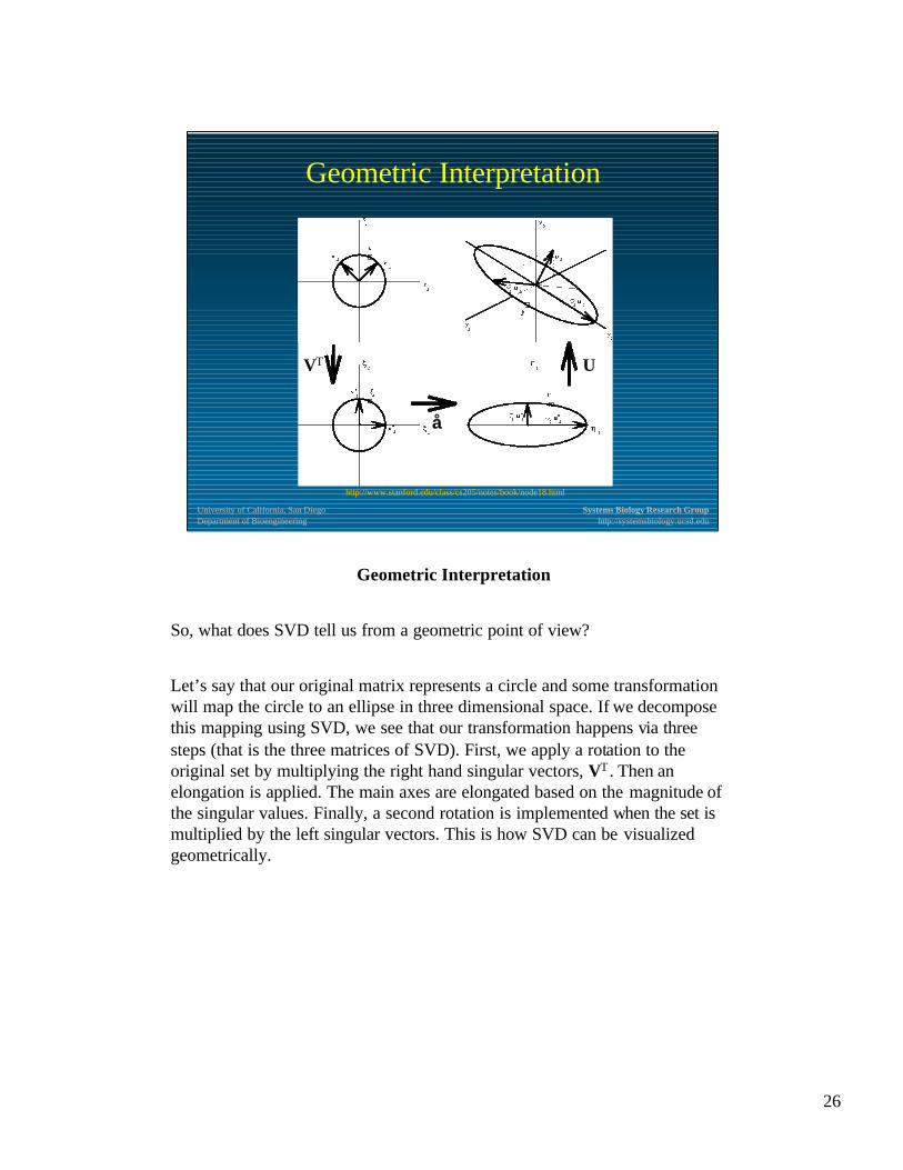
Geometric Interpretation

http://www.stanford.edu/class/cs205/notes/book/node18.html

VT U

å

Geometric Interpretation

So, what does SVD tell us from a geometric point of view?

Let’s say that our original matrix represents a circle and some transformation will map the circle to an ellipse in three dimensional space. If we decompose this mapping using SVD, we see that our transformation happens via three steps (that is the three matrices of SVD). First, we apply a rotation to the original set by multiplying the right hand singular vectors, VT . Then an elongation is applied. The main axes are elongated based on the magnitude of the singular values. Finally, a second rotation is implemented when the set is multiplied by the left singular vectors. This is how SVD can be visualized geometrically.

27



Mathematical FormulationMathematical Formulation

vTT

dtd

SVx

U =

vSx

=dtd

T

mxn

V000S

US

=

)()(

vTkk

Tk

dtd

vxu

s=

Dynamic Mass Balance Equation:

Combine (1) and (2):

(for k-=1,...,r)

SVD decomposition of S:

(1)

(2)

or

ukT

· x = uk1x1 + uk2x2 + … + ukrxm

Systemic reactions (eigen-reactions):

vkT

· v = vk1v1 + vk2v2 + … + vknvn

Systemic participation: (eigen-connectivity):

å u ki x i for u ki <0

å u ki x i for u ki >0

å v kj v j

(3)

(4)

(5)

(6)

Mathematical Formulation

So, how do we incorporate SVD analysis into stoichiometric matrix analysis? The dynamic mass balance equation (Eq. 1) describes how the temporal concentration changes of metabolites, dx/dt, are related to the flux, v, changes of chemical reactions using stoichiometric matrix as a linear transformation. S, as described, is a linear mapping between the concentration space and the flux space. Singular value decomposition of S results in the formation of the left singular vectors, uk, diagonal matrix of singular values, si, and the right singular vector, vk (Eq. 2). We can substitute Eq. 2 in Eq. 1 and rearrange the equation, which allow us to formulate systemic reactions and systemic connectivities (Eqs. 4 and 5). This means that there is a linear combination of metabolites (Eq. 4) that is being uniquely moved by a linear combination of reactions (Eq. 5). The motion that takes place via these sets of systemic reactions and connectivities are orthogonal to each other and thus are structurally decoupled.

28



Definition of Systemic Reactions:Definition of Systemic Reactions:just for illustrationjust for illustration

ukT

· x = uk1x1 + uk2x2 + … + ukrxm

a x1 + b x2 ® c x3 + d x4

Systemic reactions:

Example (for illustration):

e x5 + f x3 ® g x2 + h x6

S =

-a-bdd00

v1 v2

x1x2x3x4x5x6

0g-f0eh

u12 x2 ® u13 x3

u21 x1 ® u24 x4

u35 x5 ® u36 x6

v2

v1

0-u12u13000

U =

-u2100u2400

u1 u2 u30000u35u36

x1x2x3x4x5x6

u2

u1

...

Definition of Systemic Reactions

Any chemical reaction is a set of metabolites being converted to each other with stoichiometrically defined coefficients, a. For example, we can think of a system in which two chemical reactions proceed as shown. The chemical reaction vectors are not orthogonal to each other and they may span a space within which all the combinations of the flux values may fall. When the system is decomposed using SVD, the resulting eigen-reactions have coefficients that are different from the chemical reactions. These eigen-reactions are orthogonal to each other and therefore capture the chemical structure of S that are independent from each other. Note that the matrix shown in this example is not exact and it is presented only for illustration purposes.

29



Definition of Systemic Reactions:Definition of Systemic Reactions:just for illustrationjust for illustration

ukT

· x = uk1x1 + uk2x2 + … + ukrxm

a x1 + b x2 ® c x3 + d x4

Systemic reactions:

Example (for illustration):

e x5 + f x3 ® g x2 + h x6

S =

-a-bdd00

v1 v2

x1x2x3x4x5x6

0g-f0eh

u12 x2 ® u13 x3

u21 x1 ® u24 x4

u35 x5 ® u36 x6

v2

v1

0-u12u13000

U =

-u2100u2400

u1 u2 u30000u35u36

x1x2x3x4x5x6

u2

u1

...

Definition of Systemic Reactions

Any chemical reaction is a set of metabolites being converted to each other with stoichiometrically defined coefficients, a. For example, we can think of a system in which two chemical reactions proceed as shown. The chemical reaction vectors are not orthogonal to each other and they may span a space within which all the combinations of the flux values may fall. When the system is decomposed using SVD, the resulting eigen-reactions have coefficients that are different from the chemical reactions. These eigen-reactions are orthogonal to each other and therefore capture the chemical structure of S that are independent from each other. Note that the matrix shown in this example is not exact and it is presented only for illustration purposes.

30



Definition of Systemic ConnectivitiesDefinition of Systemic Connectivities

Example:

S =

-a-bdd00

v1 v2

x1x2x3x4x5x6

0-fg0eh

v12 v1 ® v12 v2

v21 v1 ® v24 v2

x2

x1-v11v12

VT =v21v22

v1 v2

v1v2

v 2

v 1

a x1 + b x2 ® c x3 + d x4

e x5 + f x2 ® g x3 + h x6

Systemic participations:

vkT

· v = vk1v1 + vk2v2 + … + vknvn

Definition of Systemic Connectivities

Similarly to the reactions, we can examine the metabolites and determine in what reactions they participate. In our example, the connectivity of metabolites can be examined by moving across the the rows of S. Once again, the connectivity vectors of metabolites are not orthogonal to each other. When the system is systematically decomposed using SVD, the resulting eigen-connectivities have coefficients that are different from the chemical reactions. These eigen-connectivities are orthogonal to each other and capture the structural property of S that are decoupled.

31



Key Features of SVDKey Features of SVD

• SVD is an objective and non-parametric analytical method.

• S=USVT

S=s1<u1.v1T>+ s2<u2.v2

T>+... +sr<ur.vrT>

• SV=US

S | = | •

• UTS= SVT

— S = • —

• SVD provides a solution to an eigenvalue/eigenvector problem

• SVD forms orthonormal basis sets for the four fundamental subspaces of a linear mapping

• SVD can be used to identify and biochemically characterize the dominant features of metabolic networks

Key Features of SVD

SVD is an objective and non-parametric analytical tool. A matrix can be decomposed using SVD. The reconstruction of the matrix is done through multiplication of eigenvector and scaling by the eigenvalues. The decomposition can be represented in different forms which each can be informative. These alternative representations may show how the reactions are scaled, or how the metabolites are connected in S. Also, SVD provides a systemic way of determining all the eigenvalues and eigenvectors for a matrix. It generates the orthonormal basis for the four subspace. And finally, it allows for the identification of dominant feature in metabolic network.

32



Angle Between a Pair of Vectors as a Angle Between a Pair of Vectors as a Measure of SimilarityMeasure of Similarity

cos(q) =

q = cos-1(u1.u2)

u1.u2||u1|| ||u2||

More similar

less similar

Angle Difference as a Similarity Measurement

It is possible to determine how similar two vectors are in a higher dimension by calculating the angle they make. The smaller the angle the more similar they are. This can be done by calculating the inner product of the two vectors and determining the arccosine of this number.

33



The U’s are more similar and V’s

The systemic metabolites are shared but the systemic reactions leading to these metabolites differ from one genome to another

Similarity Measure of Right and Left Similarity Measure of Right and Left Singular VectorsSingular Vectors

Similarity between the Right and Left Singular Vectors

As a means for comparing the singular vectors of different networks, the cosine angle of the vectors were measured in comparison with the singular vector of the genome-scale network of E. coli. As we can see the similarity between the singular vectors of U and V decreases as we go through the dominant modes. Another observation is that the singular vectors of U are more similar among the networks than those of V. This implies that the systemic metabolites are shared among the networks but the systemic reactions leading to them differ from one organism to another.

34



Conversion of ATP to ADP and Pi

Redox Metabolism of NADP and NADPH

Proton motive force

Metabolism of inorganic phosphate

ATP ® ADP + Pi

NADPH ® NADP

Hext

Pi and PPi

EigenEigen--Reaction SpectrumReaction Spectrum

UU

The first 4 modes

Eigen-Reaction Spectrum

If we examine the singular vectors of the U matrix for the three genome-scale networks, we’ll see that the first mode represents the conversion of ATP to ADP and Pi, the second mode shows the conversion of the redox potential, the third mode represents the proton motive force, and the fourth mode shows the phosphate metabolism in the cell.

35



AT

P-co

uple

d T

rans

port

ers

Synt

heta

se

AT

P-co

uple

d Tr

ansp

orte

rs

AT

P-co

uple

d T

rans

port

ers

Kin

ase

Kin

ase

“ATP ® ADP + P i”

EigenEigen--Connectivity Spectrum (1Connectivity Spectrum (1stst Mode)Mode)VVTT

Eigen-Connectivity Spectrum

(reactions that “collectively” drive the conversion)

We can also examine each singular vector of V that corresponds to these four singular vectors of V. The first mode delineates what reactions systemically contribute to the conversion of ATP to ADP and Pi. As you can see, a number enzymes are grouped together. In E. coli, the synthetase and ATP-coupled transporters show up together. In H. influenzae and H. pylori, ATP-coupled transporters and kinases are grouped together and contribute to this systemic conversion of ATP to ADP and Pi.

36



Red

ucta

se to

Deh

ydro

gena

se

Fatty

Aci

d Sy

nthe

sis

Red

ucta

se to

Deh

ydro

gena

se

Fatty

Aci

d Sy

nthe

sis

Red

ucta

s

Fatty

Aci

d Sy

nthe

sis

“NADPH ® NADP”

EigenEigen--Connectivity Spectrum (2Connectivity Spectrum (2ndnd Mode)Mode)VVTT


For the second mode, the systemic conversion of NADPH to NADP is done through the systemic coupling of fatty acid synthesis and reductases and dehyrogenases in E. coli and H. influenzae and fatty acid synthesis and reductases in H. pylroi.

37



H-c

oupl

ed T

rans

port

ers

ET

S ETS

ET

S

H-c

oupl

ed T

rans

port

ers

H-c

oupl

ed T

rans

port

ers

“Hext”

EigenEigen--Connectivity Spectrum (3Connectivity Spectrum (3rdrd Mode)Mode)

VVTT


The third mode corresponding to the proton motive force is media ted through the systemic grouping of electron transport system and proton-coupled transporters in all three networks.

38



Phos

phat

ase

Deh

ydro

gena

se

Fatty

Aci

d D

egre

datio

n

Synt

heta

se

Synt

ase

Phos

phat

ase

Deh

ydro

gena

se

Fatty

Aci

d D

egre

datio

n

Synt

heta

se

Synt

ase

“Pi and PPi”

EigenEigen--Connectivity Spectrum (4Connectivity Spectrum (4thth Mode)Mode)

VVTT


Finally, the phosphate metabolism is achieved through the systemic grouping of phosphatase, dehydrogenase, and fatty acid degradation in E. coli, synthetase in H. influenzae, and synthase in H. pylori.

39



• Cofactor participation in energy, redox , and phosphate metabolismconstitutes the dominant features of the metabolic networks, with a similar level of importance.

• Reactions deriving the leading features differ from one network to another.

• We can characterized dominant features of genome -scale metabolic networks that are systemically decorrelated.

• The differences among metabolic networks of living organisms are in finer details .

•We can now define systemic metabolic reactions for study of systems biology of metabolism.

What Have We Learned from the SVD What Have We Learned from the SVD Analysis of GenomeAnalysis of Genome--Scale Networks?Scale Networks?

Lessons Learned

So what have we learned from the analysis of metabolic networks using SVD?

40



The Two Null Spaces of S:Pools and Pathways

41



N(S)

v

vdyn

v ss

0 0

dtd

dyn

xC =

Cconsv

C

R(S^) R(S)

N(S^)

The Four Fundamental Subspaces of SDynamic Flux Vectors: thermodynamic state

Time Derivatives of concentrations:

Dynamic Invariants:Pools of metabolite concentrations

vss ® Svss = 0

v ® Sv

vdyn ® Svdyn = Sv

Steady State Flux Vectors:Extreme pathways

A Schematic Depiction of the Action of a Matrix and the Four Subspaces Associated With It

Every matrix can be thought of as a mapping function or a lineartransformation. It takes a vector from one space and transforms it into a vector in another space, of perhaps a different dimensionality. The four fundamental spaces are the row, column, null, and the left null spaces. These spaces are further described on the next slides.

42



The Four Fundamental Subspaces of S• The row space

– contains the dynamic flux vectors and thermodynamic transitions

• The null space– contains all the steady state solutions to the flux balance

equations

• The column space– contains the time derivatives of concentrations resulting

from the mapping

• The left null space – contains all the dynamic conserved invariants of the

network

The Four Subspaces of the Stoichiometric Matrix

All the four fundamental subspaces of S will be of interest to us. The first spaces that we will study are the right and left null space of S, since they contain all the steady state solutions, Sv = 0, and the pooled variables, Σi(dXi/dt) = 0.

43



Pools and Pathways

A* DE

E*

BA

C

POOL: CONSERVED BY FLOW IN PATHWAY

PATHWAY: CONNECTING INPUT TO AN OUTPUT

Pools and Pathways

The null space defines the space in which all the steady state solutions reside. In this space, pathways are formed which connect the network’s input(s) to its output(s), while keeping the net metabolite rates unchanged over time (i.e. dX/dt=0).

The left null space on the other hand, defines a space in which all the conserved concentration quantities reside. Here, the conserved metabolite entities form the pools whose total value stay constant in the network and does not change by the flow in the pathways.

44



The Closed “A to B” System

S =−1 11 −1

The Null Space The Left Null Space

11

p1

A B

p1

1 1( ) C1

A B

C1

+

v1

A B

v2 AkBkdtdB

BkAkdtdA

12

21

+−=

+−=

The Simple ‘AB’ Example:

Let’s consider a reversible reaction. The stoichiometric matrix S is shown, and it is rank deficient or singular.

The addition of the two columns gives zero. This can be seen by multiplying the stoichiometric matrix with the column vector (1,1)t. Thus, this column vector spans the null space. This vector represents the pathway

v1+v2

or the reversible back and forth reaction.

The addition of the rows gives a zero. This can be seen by multiplying from the left with the vector (1,1). Thus (1,1) spans the left null space and represents the summation of

A+B.

It is obvious in this case that this sum is time invariant.

45



The Open “A to B” System

v1

A B

v2

b1 b2 S =−1 1 1 01 −1 0 −1

The Null Space: The Left Null Space:

1 10 11 01 0

p1 p2

A Bp1

A B

p2

No Conservation Quantities

The Open ‘AB’ Example

If we now add exchange fluxes, the stoichiometric matrix for the closed system is ‘appended’ with the exchange reactions. The matrix is no longer rank-deficient. Thus, the left null space is of zero dimension and there are no conserved quantities. The sum of A and B will vary with time depending on the exchange fluxes.

The null space is now two-dimensional. It is spanned by two pathways. The same pathway that existed for the closed system, corresponding to the reversible reaction, is still there. Later, we shall classify this pathway as Type III.

There is a new pathway vector. It ties the input and the output via a straight pass through the system. Later, we shall classify this pathway as Type I.

Any steady state flux distribution in this simple open ‘AB’ system is a linear combination of these two basis pathways.

46



The Larger Closed “A to B” System

The ‘Smaller’ Left Null Space:

C1 = A + B

v1

A B

v2

b1 b2A* B*

The ‘Larger’ Left Null Space:

C2 = A* + A + B + B*

The Small Null Space:

1 10 11 01 0

p1p2

A Bp1

A B

p2

v1v2b1b2

p1 p2

The Larger Closed “AB” Example

If we now add the external metabolites A* and B*, the system is again closed.

47



The open “A to B to C” System

A B C S =−1 1 0 1 01 −1 −1 0 00 0 1 0 −1

p1 = (1 , 0 , 1, 1, 1)p2 = (1, 1, 0, 0, 0)

A B

p2

A B

p1

C

A Slightly More Complex Example

The next two slides contain a slight variation from the previous example. Now we are examining a 3 component system but the analysis is the same. A and B equilibrate on the fast time-scale forming a pool (A+B). On the slower time scale the the pool (A+B) is filled via the input reaction and drained via the conversion to C.

48



The Michaelis-Menten Mechanism: Open System

p1 p2

C1 = (0, 1, 1, 0)

S E+ E P+ES

p1 p3

p4p5

S E+ E P+ES

No conservation quantities

v1

v2

v3

b1

b2

b3

b4

1 1 1 1 1

0 1 0 0 0

1 0 1 1 1

1 0 1 0 0

1 0 0 1 0

0 0 0 1 1

0 0 1 0 1

p1 p2 p3 p4 p5b1 b2

b1 b2

b3 b4

The Michaelis-Menten Mechanism:

open system

Again, this slide just shows the changes in the pathway and conservation structures as a result of adding inputs and outputs to the system.

49



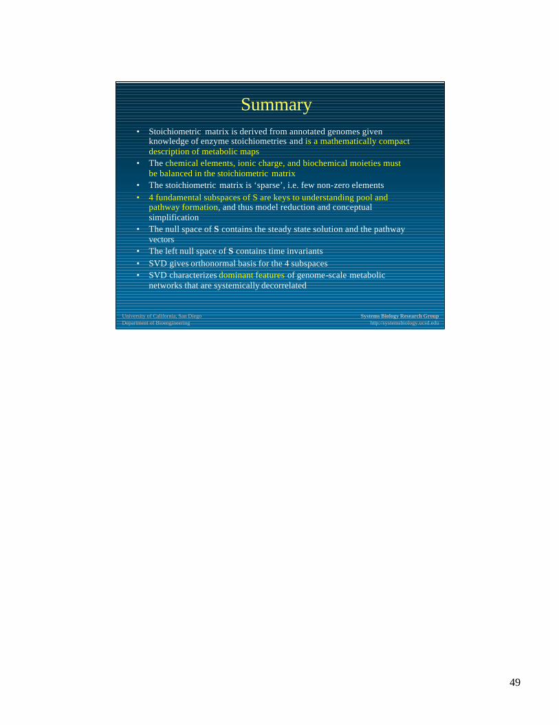
Summary• Stoichiometric matrix is derived from annotated genomes given

knowledge of enzyme stoichiometries and is a mathematically compact description of metabolic maps

• The chemical elements, ionic charge, and biochemical moieties must be balanced in the stoichiometric matrix

• The stoichiometric matrix is ‘sparse’, i.e. few non-zero elements• 4 fundamental subspaces of S are keys to understanding pool and

pathway formation, and thus model reduction and conceptual simplification

• The null space of S contains the steady state solution and the pathway vectors

• The left null space of S contains time invariants• SVD gives orthonormal basis for the 4 subspaces• SVD characterizes dominant features of genome-scale metabolic

networks that are systemically decorrelated

50



References• Ouzounis, C.A. and P.D. Karp, Global properties of the metabolic map of

Escherichia coli. Genome Research, 2000. 10(4): p. 568-76.• Edwards, J.S. and B.O. Palsson, The Escherichia coli MG1655 in silico metabolic

genotype: Its definition, characteristics, and capabilities. Proceedings of the National Academy of Sciences, 2000. 97(10): p. 5528-5533.

• Edwards, J.S. and B.O. Palsson, Systems properties of the Haemophilus influenzaeRd metabolic genotype. Journal of Biological Chemistry, 1999. 274(25): p. 17410-6.

• Schuster, S., T. Höfer, Determining all extreme semi-positive conservation relations in chemical reaction networks: a test criterion for conservativity. J. Chem. Soc. Faraday Trans. 1991. 87: p. 2561-2566.

• Meyer, C. D. Matrix analysis and applied linear algebra (Society for Industrial and Applied Mathematics, Philadelphia, 2000).

• Strang, G. Linear Algebra and its Applications (Saunders College Publishing, Fort Worth, 1988).

• Jeong, H., et al., The large-scale organization of metabolic networks. Nature, 2000. 407(6804): p. 651-4.

• Schilling, C.H. and B.O. Palsson, The underlying pathway structure of biochemical reaction networks. Proceedings of the National Academy of Sciences of the United States of America, 1998. 95(8): p. 4193-8.

51



References• Karp, P.D., Pathway Databases: A Case Study in Computational Symbolic Theories.

Science, 2001. 293(5537): p. 2040-2044. Alter, O., Brown, P. O. & Botstein, D. Singular value decomposition for genome-wide expression data processing and modeling. Proceedings of the National Academy of Sciences of the United States of America 97, 10101-6 (2000).

• Holter, N. S. et al. Fundamental patterns underlying gene expression profiles: simplicity from complexity. Proceedings of the National Academy of Sciences of the United States of America 97, 8409-14 (2000).

• Nielsen, T.O. et. al. Molecular characterization of soft tissue tumors: a gene expression study, Lancet. 2002 Apr 13;359(9314):1301-7.

• Fogolari F, Tessari S, Molinari H. Singular value decomposition analysis of protein sequence alignment score data. Proteins. 2002 Feb 1;46(2):161-70.

• Famili, I and B. O. Palsson, Systemic Metabolic Reactions Are Obtained by Singular Value Decomposition of Genome-Scale Stoichiometric Matrices, in review.

• B. O. Palsson, "On the Dynamics of the Irreversible Michaelis-Menten Reaction Mechanism'', Chem. Eng. Sci., 42, 447-458 (1987).

• C.H. Schilling, S. Schuster, B.O. Palsson, and R. Heinrich, "Metabolic Pathway Analysis: Basic Concepts and Scientific Applications in the Post -Genomic Era," Biotechnology Progress, 15: 296-303 (1999).

• Reinhart Heinrich and Stefan Shuster, The Regulation of Cellular Systems, Chapman and Hall, New York, 1996.

• David Lay, Linear Algebra and its Applications, Addison-Wesley, Menlo Park, 1997.

Documents

Representing Reconstructed Networks Mathematically: The ...systemsbiology.ucsd.edu/sites/default/files/Attachments/Images/... · Representing Reconstructed Networks Mathematically: