Embed Size (px)
Citation preview
Universiteit van Amsterdam
MSc Mathematical Physics
Master Thesis
Representations of Uq(sl2∣1)at roots of unity
Tim Weelinck
June 26, 2015
Supervisor:Prof. Dr. N.R.Reshetikhin
Second Reader:Dr. H.B. Posthuma
Korteweg-de Vries Instituut voor WiskundeFaculteit der Natuurwetenschappen, Wiskunde en Informatica

Representations of Uq(sl2∣1)at roots of unity
Tim Weelinck
AbstractIn this thesis representations of Uq(sl2∣1) at roots of unity are studied. The
representation theory is studied by applying techniques and methods developedby C. De Concini, V. Kac and C. Procesi for quantum groups at roots of unity
[DCK90, DCKP92].The study of simple representations of Uq(sl2∣1) is reduced to the study of a
family, Ax, of finite dimensional quotients of Uε(sl2∣1) parametrized by an affinevariety Ω = Spec(Z0). Here Z0 is some central sub-Hopf algebra of Uε(sl2∣1). It isshown that Z0 has a canonical Poisson bracket, inducing an isomorphism betweenPoisson manifolds Ω and (SL∗
2∣1)∅, the base space of the dual Poisson-Lie group.
An action of an infinite group on Ω is defined, the so-called quantum coadjointaction. It is shown that orbits of the quantum coadjoint action are exactly thesymplectic leaves in Ω. It is deduced that Ax is generically semimsimple over Ω
by concretely describing the generic simple representations. Moreover, it isshown that the family of algebras Ax can be seen as a trivial vector bundle overΩ, and that for two points x, y in the same symplectic leaf we have that Ax is
isomorphic to Ay as algebras.
II

AcknowledgementsFirst and foremost, I would like to thank my supervisor Nicolai Reshetikhin. I amthankful for the time taken supervising this project and the wealth of ideas -andnew approaches- he shared with -and suggested to- me. I am also thankful forpleasant conversations on visions on mathematics, and life in and outside of math.
Secondly, I wish to thank Hessel Posthuma for being second reader, and forhelpful discussions on Poisson geometry.
Thirdly, I want to give my thanks to Sacha, Iordan and David for fruitfulconversations while in Berkeley.
Fourthly, I want to thank all the students at KdV for enjoyable coffee breaks,lunches, and especially Reinier for assisting me geometrically.
Lastly, I want to express my sincerest gratitude towards Juultje, for everything.
III


Contents
Abstract II
Acknowledgements III
Introduction 1
1 Preliminaries on Quantum Supergroups 71.1 Hopf superalgebras and enveloping superalgebras . . . . . . . . . . . 71.2 Superbialgebras and Poisson-Lie supergroups . . . . . . . . . . . . . . 171.3 Uq(sl2∣1) as quantization of O(SL∗
2∣1) . . . . . . . . . . . . . . . . . . . 26
2 Representation Theory of Uε(sl2∣1) 352.1 Structure of the Quantized Universal Enveloping Lie Superalgebra . 352.2 Generic representations of Uε(sl2) . . . . . . . . . . . . . . . . . . . . . 402.3 Generic Representations of Uε(sl2∣1) . . . . . . . . . . . . . . . . . . . . 412.4 Sets of irreducible representations parametrized over the dual Pois-
son Lie group . . . . . . . . . . . . . . . . . . . . . . . . . . . . . . . . . 44
3 The Quantum Coadjoint Action 493.1 A canonical Poisson structure on Z0 . . . . . . . . . . . . . . . . . . . 493.2 The quantum coadjoint action . . . . . . . . . . . . . . . . . . . . . . . 543.3 Geometry of the quantum coadjoint action . . . . . . . . . . . . . . . 603.4 Structure of Ax as vector bundle over Ω . . . . . . . . . . . . . . . . . 65
Discussion 69Discussion . . . . . . . . . . . . . . . . . . . . . . . . . . . . . . . . . . . . . . 69Future work . . . . . . . . . . . . . . . . . . . . . . . . . . . . . . . . . . . . . 69
A A Short Introduction to Super Mathematics 71A.1 Basics on Lie superalgebras . . . . . . . . . . . . . . . . . . . . . . . . . 71A.2 Supermanifolds . . . . . . . . . . . . . . . . . . . . . . . . . . . . . . . . 76A.3 Lie supergroups . . . . . . . . . . . . . . . . . . . . . . . . . . . . . . . . 81
V

VI
B PBW Theorems 85
C Representation Theory of Semisimple Algebras 89
D A very short introduction to Spec(R) 99
E Quantum Calculus 103
Bibliography 110

Introduction
In this thesis we study the representation theory of the quantum supergroupUq(sl2∣1) at roots of unity. We should add that Uq(sl2∣1) is not really quantum, noris it a supergroup. What then, is Uq(sl2∣1)? To answer this question we will jumpback in time to the early 80s.Theoretical physicsts were studying the quantum inverse scattering method (QISM),a method to solve quantum integrable systems developed by Ludvig Faddeev andhis group at the Leningrad School. In 1981 Petr Kulish and Nicolai Reshetikhin[KN83] described what would later be recognized as Uq(sl2), the first example ofa quantized universal enveloping algebra.We refer to chapter one to learn what is meant by ‘universal enveloping algebra’.We will take some time to explain the term ‘quantized’. Nowadays, the wordhas its own meaning in mathematics, but this is of course a term borrowed fromphysics. Let us start with the physics and then distill from it what we shall meanwith quantization.
Intermezzo: quantizationIn the early 20th century physics was split into two seemingly separateworlds: the classical (macroscopic) world and the quantum (smallest scale)world. To describe a physical system in classical mechanics, one specifiescertain data: a smooth Poisson manifold M playing the role of the spaceof possible states, and a set of observables, which are functions on themanifold M . The evolution of the system over time is represented by asmooth path m(t) in M . Given a starting point m(t0), the following setof equations
d
dtf(m(t)) = Hcl, f(m(t))
determines the evolution of m(t) over time. Here Hcl denotes some specialfunction called the classical Hamiltonian, and ⋅, ⋅ denotes the Poissonbracket.In quantum mechanics, one specifies similar data, but the mathematicalstructures are different. The space of states is now a complex Hilbert space,and the observables are non-commutative operators on the Hilbert space.A special operator, called the quantum Hamiltonian Hqu, now encodes the
1

2
time evolution of an operator A as follows
dA
dt= [Hqu,A]
Can one pass from the classical situation to a the quantum situation? Thisis exactly the problem of quantization. One approach, due to Jose Moyal,is to keep the space of functions on the manifold as space of observables,but to replace the product between functions by some non-commutativeproduct. Let us make this more precise: denote F(M) the set of functionson M , and denote ⋆0 the normal commutative product on F(M). Wedefine a family of products ⋆h depending on some parameter h (h can bea complex number for example), such that ⋆0 is the old product, and ⋆hsatisfies some smoothness condition with respect to h. One should think ofh as Planck’s constant. As Planck’s constant tends to 0, h → 0, quantummechanics becomes classical mechanics, and from Physical motivation weask that
limh→0
f ⋆h g − g ⋆h f
h= f, g (*)
Of course a mathematician does not need to restrict its attention to func-tion algebras on spaces of states, one can consider any commutative algebraA with a Poisson bracket and wonder whether we can deform the productto some product ⋆h satisfying (∗). This is what we will mean by a ‘quan-tizations’.1
Returning to Kulish and Reshetikhin, it was later realized they had defined afamily of algebras Uq(sl2), dependent on some complex parameter q, that shouldalso be considered as a quantization. Mid 1980’s Vladimir Drinfel’d and Mi-chio Jimbo independently generalized the construction of Uq(sl2), by associat-ing a quantum group Uq(g) to any simple Lie group g. In his famous address[Dri87] in 1986 in Berkeley, Drinfel’d popularized the name ‘quantum group’ forthese objects. Drinfel’d developed the basis for the theory of quantum groups,introducing concepts such as Poisson-Lie groups and Lie bialgebras. Althoughquantum groups were initially conceived to produce non-trivial solutions to theYang-Baxter equation, nowadays they are connected to many diverse mathemati-cal fields.2 For example, quantum groups have become connected to knot theoryand low-dimensional topology, most famously perhaps in the construction of therenowned Reshetikin-Turaev invariants [RT91].
In the early 90s Victor Kac, Corrado De Concini and Claudio Procesi publisheda series of papers studying the properties of quantum groups at roots of unity,
1This of course does not constitute a rigorous definition, but it is the right idea. See definition1.2.3 for an improved definition.
2The Yang-Baxter equation is an important equation in QISM.

3
amongst others [DCK90, DCKP92], and an enlarged summary in [DCP93]. Byutilizing methods from smooth and algebraic geometry they were able to lay baremany interesting properties of the representation theory of the quantum group atroots of unity. This thesis should be seen as a direct succesor to the ideas in thesepapers. We consider a specific quantum supergroup and utilize the techniquesdeveloped by De Concini, Kac and Procesi to study its representation theory.
The purpose of this project is twofold. Firstly, we show that many of the techniquesand methods developed in [DCK90, DCP93, DCKP92] are almost directly appli-cable to Uq(sl2∣1). This gives strong evidence that the same should hold for moregeneral basic Lie superalgebras. Secondly, although the papers [DCK90, DCKP92]have a certain status in the field, the author has found that many PhD studentsworking in areas closely related to quantum groups have not actually read thesepapers themselves.The author conjectures that the style of writing of these papers has a lot to dowith that. To illustrate this point, an important result in [DCP93, prop. 11.8]which has but four lines as proof, has grown in size to a proof of more than a pagein this thesis as proposition 3.4.1. We do not believe this difference in size is dueto a misunderstanding of the theorem or its proof.The author has modest hopes that by providing a detailed ‘worked example’ inthis thesis, the original work of De Concini, Kac and Procesi becomes accesible toa wider audience.
Organisation and main results
The thesis is written having a first year master student, or advanced undergraduatestudent, in mind as audience. We hope the style does not come across as pedantic,but we have tried to consistently choose clarity over brevity. We hasten to addthat this holds for the ‘main part’ of the thesis, being chapter two and three. Wehave added chapter one to provide a fuller picture to the reader, but the chapteris in no way meant as a comprehensive introduction to quantum supergroups.
Chapter One: Preliminaries on Quantum Supergroups
This chapter is written with two goals in mind. On the one hand, we try to getthe reader up to speed with quantum supergroups. We introduce the mathemat-ical definitions underlying the object Uq(sl2∣1) such as super Hopf algerbras, Liesuperbialgebras and Poisson-Lie supergroups. The treatment is rather brief, butreferences are provided on all important topics.On the other hand, the chapter is written to make precise in what way Uq(sl2∣1)quantizes what Poisson manifold. If the reader is to take anything from the chapterit should be the following statement.

4
• Uq(sl2∣1) endows O(SL∗2∣1
) with the structure of a Poisson-Hopf algebra.
Hence O((SL∗2∣1
)∅) also has the structure of a Poisson-Hopf algebra.
Chapter Two: Representation Theory of Uε(sl2∣1)
We study Uq(sl2∣1) at a root of unity. We prove the following structure theoremsin section one.
• Let ε be an `th root of unity. Uε(sl2∣1) has a central sub-Hopf algebra Z0
generated by the `th powers of the even generators.
• Uε(sl2∣1) is a free Z0-module of dimension 16`4.
In the second and third section we define a family of Uε(sl2∣1)-modules dependenton a set of four parameters living in C2 ×C∗2. Excluding some Zariski closed setin C2 ×C∗2 this family consists of `2 non-isomorphic simple modules of dimension4`.In the fourth section we prove that
Z0 ≅ O((SL2∣1)∅) (*)
as Hopf algebras. This allows us to study representations of Uε(sl2∣1) over the affinevariety Ω ∶= maxSpec(Z0) ≅ (SL∗
2∣1)∅. In particular we identify the parameters
that defined a family of representations, as points in Ω, and prove the followingtheorem.
• There exists a Zariski open subset of Ω such that Ax ∶= Uε/mxUε is a semisim-ple algebra of dimension 16`4 over those points.3 The semisimple algebrasplits up as a direct sum of `2 simple modules of dimension 4`.
Chapter Three: The Quantum Coadjoint Action
We begin this chapter by substantially improving the isomorphism *, with thefollowing result.
• Z0 has a canonical Poisson bracket defined by
a, b = limq→ε
ab − ba
`(q` − q−`)
this endows Z0 with the structure of a Poisson-Hopf algebra and as Poisson-Hopf algebras Z0 ≅ O((SL∗
2∣1)∅).
Now that Ω is endowed with a Poisson structure, we wish to study the interactionbetween Poisson geometry and representation theory. In section two we prove thefollowing results.
3Here mx denotes the maximal ideal corresponding to a point x ∈ Ω = Spec(Z0).

5
• We can naturally associate a Lie algebra g of complete vector fields on Ω tothe generators of Z0.
• The global flows corresponding to the complete vector fields in g define aninfinite group G acting on Ω (the quantum coadjoint action). The orbits ofG are are exactly the symplectic leaves of Ω.
In section three we elucidate the structure of the symplectic leaves, by proving thefollowing results
• There exists a natural 4-1 covering map π from Ω to the big cell G0 ⊂
(SL2∣1)∅.
• The Lie algebra generated by the infinitesimal generators of the conjugationaction of (SL2∣1)∅ lift to a Lie algebra of vector fields g on Ω.
• At every point of Ω we have that g and g span the same space in the tangentspace to Ω.
• Let O denote a conjugacy class in SL2∣1. Then O0 = G0 ∩ O is a smoothconnected variety and the connected components of π−1(O0) are orbits of thegroup G.
Hence, we can use the structure of conjugacy classes in (SL2∣1)∅ to study thesymplectic leaves in Ω. For example, we immediately obtain the structure of thefixed points of G.
• Denote F the fixed points of G, then F = (z1, z2, b, c) ∈ Ω ∶ z1 = 1, b = c = 0.
The last section is devoted to proving the following important theorem
• The family of algebras Ax ∶= Uε(sl2∣1)/mxUε(sl2∣1) defines a trivial vectorbundle of rank 16`4 over Ω. For two points x, y in the same sympletic leafwe have that Ax ≅ Ay as algebras.
Appendices
In the appendices we have placed the theory that we could not give a satisfyingplace within the thesis.
Appendix AThe first three appendices give a short introduction to super mathematics, andare intended to provide the necessary background knowledge to read chapter one.Similar to the approach in chapter one, many results are stated without proof, butrather are references provided.

6
Appendix BThe appendix on the PBW theorem, provides a brute force proof of the PBWtheorem for Uq(sl2∣1).
Appendix CThe appendix on representation theory is a compact introduction to Jacobson the-ory of semisimple algebra, culminating in the proof of the following statement
Let A be a finite dimensional algebra of dimension n, let Mi be a set of non-isomorphic simple modules of A such that dim(A) = ∑i dim(Mi)
2. Then
1. A is a semimsimple algebra.
2. A ≅∏i End(Mi) as algebra.
3. Mi constitute a complete set of simple modules.
The material in this appendix is standard and can be found in many books,for example [Lan02]. However, the proof of theorem C.0.35 is original, in the sensethat the author is unaware of a similar proof in the literature.
Appendix DThe introduction on Spec(R) was written with the student in mind who has neverattended a course on algebraic geometry. The appendix is rather brief, as we donot need much algebraic geometry.
Appendix EThe final appendix deals with quantum calculus, whose identities we will need atseveral points of the thesis. We have chosen to give a elaborate introduction there,more than necessary at least, mainly because we feel q-calculus is a lot of fun toplay around with.

Chapter 1
Preliminaries on QuantumSupergroups
In this first chapter we will introduce the concepts that are preliminary to theobject that we wish to study: the quantum supergroup Uq(sl2∣1). We have triedto introduce those concepts that a ‘generic first year graduate student’, will notbe familiar with. For basics on super mathematics we refer to the appendix. Incontrast with the rest of the thesis the emphasis will be on stating results withoutproof, instead providing references. The idea being that the this section createscontext and motivation for the further thesis, but is not vital to appreciating therepresentation theoretic results in the rest of the thesis. The main goal of thischapter can be summarized as: explaing what it means that the super Hopf algebraUq(sl2∣1) quantizes O(SL∗
2∣1).
1.1 Hopf superalgebras and enveloping superal-
gebras
A Hopf algebra is an algebra that has a compatible structure as a coalgebra.Moreover, a Hopf algebra is endowed with a special antihomomorphism. Theynaturally appear as the function algebras on (smooth, algebraic) groups.
Historical Remark. In [Dri87] Drinfel’d writes that quantum groups are more or lessthe same as Hopf algebras. Unfortunately, there is still no satisfactory definition ofquantum group today. Drinfel’d reasons as follows. If one considers a group (Liegroup resp. algebraic group) the (smooth resp. regular) functions on that groupnaturally have the structure of a commutative Hopf algebra. In fact this gives ananti-equivalence of categories, if one matches the right type of group to the right
7

8 Preliminaries on Quantum Supergroups
type of Hopf algebra. The non-commutative Hopf algebras are to be consideredas non-commutative functions on a ‘quantum group’.
A thorough treatment of Drinfel’ds philosophy would require too much space.Instead, we will define the central concepts of super Hopf algebra, Lie superbialge-bra and Poisson-Lie supergroup and work out the example of how the super Hopfalgebra Uq(sl2∣1) quantizes the function algebra O(SL∗
2∣1).
Remark. Super Hopf algebras are simple generalizations of Hopf algebras. Readersfamiliar with Hopf algebras and universal enveloping algebras are advised to skipto the end of this section.
The part ‘co’ in coalgebra refers to a dual structure. In this case a dualizedalgebra structure, similarly supercoalgebras are dual superalgebras.1 We give adefinition of superalgebra different from the one in the appendix, because it iseasier to dualize.
Definition 1.1.1. An associative superalgebra with unit is a triple (A,µ, η) whereA is a super vector space and two even linear maps, the product µ ∶ A⊗A→ A andthe unit η ∶ C→ A, satisfying the conditions (Un) and (Ass).(Un) The diagram
A⊗A⊗A A⊗A
A⊗A A
id⊗ µ
µ⊗ id
µ
µ
commutes.(Ass) The diagram
C⊗A A⊗A A⊗C
A
η ⊗ id id⊗ η
≅ ≅
commutes.A superalgebraA is called (super)commutative if, in addition, the condition (Comm)holds(Comm) The diagram
1We follow common terminology, and thus resist to write cosuperalgebra.

Hopf superalgebras and enveloping superalgebras 9
A⊗A A⊗A
A
τ
η η
commutes.Here τ ∶ A⊗A→ A⊗A is the graded flip, defined by τ(a⊗ b) = (−1)∣a∣∣b∣b⊗ a.
A morphism of superalgebras f ∶ (A,µ, η) → (A′, µ′, η′) is an even linear mapf ∶ A→ A′ such that
η′ (f ⊗ f) = f η and f η = η′.
Example 1.1.2. Let V be a super vector space. We define super vector spaceT (V ) = ⊕n>0T n(V ), where T 0(V ) = C, T n(V ) = V ⊗n for n > 0. The canonicalisomorphisms T n(V )⊗Tm(V ) ≅ T n+m(V ) induce an associative product on T (V )
explicitly given by
(x1 ⊗ . . .⊗ xn) ⋅ (xn+1 ⊗ . . . xn+m) = x1 ⊗ . . .⊗ xn+m.
We call this the tensor algebra of V .
The definition of superalgebra is readily dualized by reversing all arrows.
Definition 1.1.3. A coassociative supercoalgebra with counit is a triple (C,∆, ε)where C is a super vector space and two even linear maps, the coproduct ∆ ∶ C →C⊗C and the counit ε ∶ C → C, such that the conditions (Coun) and (Coass) hold.(Coun) The diagram
C⊗C C ⊗C C ⊗C
C
ε⊗ id id⊗ ε
∆≅ ≅
commutes.(Coass) The diagram
C C ⊗C
C ⊗C C ⊗C ⊗C
∆
∆ id⊗∆
∆⊗ id

10 Preliminaries on Quantum Supergroups
commutes.A supercoalgebra C is called co(super)commutative if the condition (Cocomm)holds.2
(Cocomm) The diagram
C ⊗C C ⊗C
C
τ
∆∆
commutes.A morphism of supercoalgebras f ∶ (C,∆, ε) → (C ′,∆′, ε′) is an even linear mapf ∶ C → C ′ such that
(f ⊗ f) ∆ = ∆′ f and ε′ f = ε.
Remark. (i) Note that in the definitions of supercoalgebra and superalgebra weare interpreting C as C1∣0. Here C1∣0 denotes the super vector space with even partC1∣0
0 = C and odd part C1∣01 = 0. In particular we ask that η(C) ⊂ A0 and that
ε(C1) = 0.(ii) To any (co)superalgebra we can associate two natural (co)algebras. Firstly,since all defining maps are even, (A0, µ, η) resp. (C0,∆, ε) define an algebra resp.coalgebra. However, using again that all maps are even, we can also define thealgebra (A/A1, µ, η) resp. coalgebra (C/C1,∆, ε). These do not define the same(co)algebras in general.3 This observation is closely related to the fact that for asupermanifold (M,A) the algebra C∞(M) is not a subalgebra of A(M) in general,but rather a quotient.
Example 1.1.4. [Kas95, p. 41](i) (Dual Coalgebra) If (C,∆, ε) is a supercoalgebra, then C∗ =HomC(C,C) natu-rally carries a superalgebra structure. Denote λ ∶ C∗⊗C∗ → (C ⊗C)∗, the naturalmap defined by λ(f ⊗ g)(v ⊗ u) ∶= f(u)⊗ g(v), τ the graded flip.Then (C∗,∆∗ λ τ, ε∗) is a superalgebra.(ii) (Dual Algebra) Let (A,µ, η) be a finite dimensional superalgebra. Then λ ∶
A∗⊗A∗ → (A⊗A)∗ is an isomorphism. A∗ has a natural supercoalgebra structuredefined by (A∗, τ λ−1 µ∗, η∗).
Notation. (Sweedler’s sigma notation) Let (C,∆, ε) be a supercoalgebra. For x ∈ Cthe element ∆(x) ∈ C ⊗C is of the form
∆(x) =∑i
x′i ⊗ x′′
i .
2We will always drop the super in cosupercommutative. For example, we will speak of co-commutative supercoalgerbas.
3In fact we can improve these associations to functors from the category of (co)superalgebrasto the the category of (co)algebras.

Hopf superalgebras and enveloping superalgebras 11
Henceforth, we shall agree to drop the subscripts and write
∆(x) =∑(x)
x′ ⊗ x′′
instead.Coassociativity allows us to unamibiguously write
∆⊗ id ∆(x) = id⊗∆ ∆(x) =∑(x)
x′ ⊗ x′′ ⊗ x′′′,
and in fact using coassociativity repeatedly allows us to use the same notation forhigher powers of the coproduct. Using Sweedler’s sigma notation we can rewritethe conditions (Coun) and (Cocomm) in the following short form:
∑(x)
ε(x′)x′′ =∑(x)
ε(x′′)x′ = x ∀x ∈ C, (Coun)
∑(x)
x′ ⊗ x′′ =∑(x)
(−1)∣x′∣∣x′′∣x′′ ⊗ x′ ∀x ∈ C. (Cocomm)
If a super vector space has both superalgebra and supercoalgebra structureswe can ask for two natural compatility conditions.
Definition 1.1.5. A superbialgebra is a quintuple (B,µ, η,∆, ε) such that (A,µ, η)is a superalgebra and (B,∆, ε) is a supercoalgebra and one of the following equiv-alent conditions holds
• ∆ and ε are superalgebra morphisms.
• µ and η are supercoalgebra morphisms.
Proof. The proof can be made entirely visual, by drawing the four commutingdiagrams that correspond to each condition and observing they are the same fourdiagrams[Kas95, th. 3.2.1].
Using Sweedler’s notation we can reformulate the first condition into the fol-lowing short form:
∑(xy)
(xy)′ ⊗ (xy)′′ = ∑(x)(y)
(−1)∣y′∣∣x′′∣x′y′ ⊗ x′′y′′,
∆(1) = 1⊗ 1, ε(xy) = ε(x)ε(y), ε(1) = 1.
Example 1.1.6. [Kas95, p. 46-47](i)Let V be a super vector space, there exists a unique superbialgebra structureon the tensor algebra T (V ) such that ∆(v) = v ⊗ 1 + 1 ⊗ v and ε(v) = 0 for anyelement v ∈ V . It is cocommutative.(ii) (Dual Bialgebra) Let B be a finite dimensional superbialgebra. Then the dualspace B∗ naturally has the structure of a superbialgebra.

12 Preliminaries on Quantum Supergroups
Definition 1.1.7. A Hopf superalgebra is a sextuple (H,µ, η,∆, ε, S) such that(H,µ, η,∆, ε) is a superbialgebra and S ∶H →H is an even linear anti-homomorphismof superalgebras satisfying the condition (An-Po)(An-Po)The diagram
H ⊗H H ⊗H
H C H
H ⊗H H ⊗H
S ⊗ id
id⊗ S
∆
∆
µ
µ
ε η
commutes.We can reformulate the condition (An-Po) in compact Sweedler’s notation:
∑(x)
S(x′)x′′ =∑(x)
x′S(x′′) = ε(x)η(1), ∀x ∈H. (An-Po)
Remark. Let (B,µ, η,∆, ε) is a superbialgebra. The bialgebra structure has im-portant consequences for the representation theory of B. The algebra B has atrivial module C on which B acts through ε. Moreover, let M,N be A-modules.Then ∆ makes M ⊗ N into an B-module, by b ⋅m ⊗ n = b′m ⊗ b′′n. Rephrasedcategorically, Mod(B), the category of B-modules, can be given the structure ofa monoidal category [KRT97, §2.1].
Example 1.1.8. (i) (Group algebra) This group algebra is not a super Hopf alge-bra, but nevertheless a very important Hopf algebra. Let G be a finite group. Thegroup algebra C[G] is defined as the C vector space with basis δgg∈G. The unitη ∶ C C[G] is given by η(c) = cδe. The product is defined by bilinearly extendingδg ⋅ δh = δgh, associativity of G makes this into an associative product. We can en-dow C[G] with a cocommutative Hopf algebra structure by letting ∆(δg) = δg⊗δg,ε(δg) = 1 and S(δg) = δg−1 .(ii) As a dual vector space k[G]∗ = Fun(G) is naturally a commutative bialgebra.We can give it antipode S∗. By interpreting Fun(G) ⊗ Fun(G) as functions onG ×G we see that coproduct, counit and antipode are given by
∆(f)(g ⊗ h) = f(gh), ε(f) = f(e), S(f)(g) = f(S(g)) = f(g−1). (1.1)
Hopf superalgebras and enveloping superalgebras 13
(iii) Let H be a finite dimensional super Hopf algebra. The dual superbialgebraH∗ is naturally a super Hopf algebra with antipode S∗.
As indicated in the following proposition, example (ii) has a very important‘extension’ to Lie- and algebraic groups.
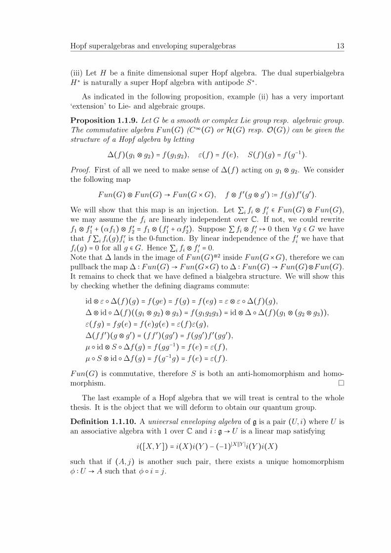
Proposition 1.1.9. Let G be a smooth or complex Lie group resp. algebraic group.The commutative algebra Fun(G) (C∞(G) or H(G) resp. O(G)) can be given thestructure of a Hopf algebra by letting
∆(f)(g1 ⊗ g2) = f(g1g2), ε(f) = f(e), S(f)(g) = f(g−1).
Proof. First of all we need to make sense of ∆(f) acting on g1 ⊗ g2. We considerthe following map
Fun(G)⊗ Fun(G)→ Fun(G ×G), f ⊗ f ′(g ⊗ g′) ∶= f(g)f ′(g′).
We will show that this map is an injection. Let ∑i fi ⊗ f′
i ∈ Fun(G) ⊗ Fun(G),we may assume the fi are linearly independent over C. If not, we could rewritef1 ⊗ f ′1 + (αf1)⊗ f ′2 = f1 ⊗ (f ′1 + αf
′
2). Suppose ∑ fi ⊗ f ′i ↦ 0 then ∀g ∈ G we havethat f ∑i fi(g)f
′
i is the 0-function. By linear independence of the f ′i we have thatfi(g) = 0 for all g ∈ G. Hence ∑i fi ⊗ f
′
i = 0.Note that ∆ lands in the image of Fun(G)⊗2 inside Fun(G×G), therefore we canpullback the map ∆ ∶ Fun(G)→ Fun(G×G) to ∆ ∶ Fun(G)→ Fun(G)⊗Fun(G).It remains to check that we have defined a bialgebra structure. We will show thisby checking whether the defining diagrams commute:
id⊗ ε ∆(f)(g) = f(ge) = f(g) = f(eg) = ε⊗ ε ∆(f)(g),
∆⊗ id ∆(f)((g1 ⊗ g2)⊗ g3) = f(g1g2g3) = id⊗∆ ∆(f)(g1 ⊗ (g2 ⊗ g3)),
ε(fg) = fg(e) = f(e)g(e) = ε(f)ε(g),
∆(ff ′)(g ⊗ g′) = (ff ′)(gg′) = f(gg′)f ′(gg′),
µ id⊗ S ∆f(g) = f(gg−1) = f(e) = ε(f),
µ S ⊗ id ∆f(g) = f(g−1g) = f(e) = ε(f).
Fun(G) is commutative, therefore S is both an anti-homomorphism and homo-morphism.
The last example of a Hopf algebra that we will treat is central to the wholethesis. It is the object that we will deform to obtain our quantum group.
Definition 1.1.10. A universal enveloping algebra of g is a pair (U, i) where U isan associative algebra with 1 over C and i ∶ g→ U is a linear map satisfying
i([X,Y ]) = i(X)i(Y ) − (−1)∣X ∣∣Y ∣i(Y )i(X)
such that if (A, j) is another such pair, there exists a unique homomorphismφ ∶ U → A such that φ i = j.
14 Preliminaries on Quantum Supergroups
We summarize some of the properties of the universal enveloping algebra inthe following theorem.
Theorem 1.1.11. [Mus12] Let g be a Lie superalgebra.
1. U = U(g) exists and equals the associative superalgebra T (g)/I where I isthe ideal in the tensor algebra T (g) generated by elements of the form X ⊗
Y − (−1)∣Y ∣∣X ∣Y ⊗X − [X,Y ] where X,Y ∈ g.
2. Any g-representation has a unique structure as a U(g)-module.
3. Let X1, . . . ,Xn be a basis of g0 over C, and Xn+1, . . . ,Xn+m a basis of g1 overC. The set Xj1
1 ⋯Xjn+mn+m with j1, . . . , jn ∈ N, jn+1, . . . , jn+m ∈ 0,1 defines a
basis of Ug over C.
4. U(g) has a canonical structure as a Hopf algebra where ∆ and ε are definedon g U(g) by
∆(X) =X ⊗ 1 + 1⊗X, ε(X) = 0, S(X) = −X.
Remark. It is not hard to check that the algebra we define in (1) has the rightproperties. The basis in (3) is called the PBW-basis, see appendix B, and showsg injects into U(g). To prove (2) and (4) one uses the universal property of U .
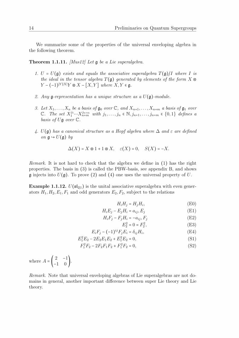
Example 1.1.12. U(sl2∣1) is the unital associative superalgebra with even gener-ators H1,H2,E1, F1 and odd generators E2, F2, subject to the relations
HiHj =HjHi, (E0)
HiEj −EjHi = aij,Ej (E1)
HiFj − FjHi = −aij, Fj (E2)
E22 = 0 = F 2
2 , (E3)
EiFj − (−1)ijFjEi = δijHi, (E4)
E21E2 − 2E2E1E2 +E
21E2 = 0, (S1)
F 21F2 − 2F2F1F2 + F
21F2 = 0, (S2)
where A = (2 −1−1 0
).
Remark. Note that universal enveloping algebras of Lie superalgebras are not do-mains in general, another important difference between super Lie theory and Lietheory.

Hopf superalgebras and enveloping superalgebras 15
Definition 1.1.13. (The Quantum Supergroup Uq(sl2∣1)) Let Uq denote the quan-tum supergroup Uq(sl2∣1), defined to be the C-superalgebra, dependent on param-eter q ∈ C∗ ∖ ±1, and having even generators K±
1 ,K±
2 ,E1, F1 and odd generatorsE2, F2, subject to the following relations
KiK−1i = 1, KiKj =KjKi, (E0)
KiEj = qaijEjKi, KiFj = q
−aijFjKi, where A = (2 −1−1 0
) , (E1)
EiFj − (−1)ijFjEi = δijKi −K−1
i
q − q−1, (E2)
E22 = 0 = F 2
2 , (E3)
E21E2 − (q + q−1)E1E2E1 +E2E
21 = 0, (S1)
F 21F2 − (q + q−1)F1F2F1 + F2F
21 = 0. (S2)
In the following proposition, we show that we can endow Uq with a super Hopfalgebra structure.
Proposition 1.1.14. There exist unique even algebra morphisms ε ∶ U → C, ∆ ∶
U → U ⊗ U , and a unique even algebra anti-morphism S ∶ U → U that are definedon the generators of Uq as follows:
∆(Ei) = Ei ⊗Ki + 1⊗Ei, ε(Ei) = 0,
∆(Fi) = Fi ⊗ 1 +K−1i ⊗ Fi, ε(Fi) = 0,
∆(Ki) =Ki ⊗Ki ε(K±1i ), = 1,
S(Ei) = −EiK−1i ,
S(Fi) = −KiFi,
S(Ki) =K−1i .
Denote µ and η the product and unit in Uq. The sextuple (Uq, µ, η,∆, ε, S) is asuper Hopf algebra.
Proof. The proof of a statement such as ‘algebra A with these generators andrelations can be given a Hopf algebra structure’ are standard. We will give anelaborate description. First we will show that existence implies uniqueness. Weknow that a general element in Uq can written as the sum of monomials a = ai1⋯ainwith aij generators. Suppose there exist two algebra morphisms ∆,∆′ defined ongenerators as above. The computation
∆(a) = ∆(ai1)⋯∆(ain) = ∆′(ai1)⋯∆′(ain) = ∆(a′)

16 Preliminaries on Quantum Supergroups
shows that ∆ and ∆′ are equal on all monomials in A, and hence equal on all ofA. The proofs that existence of ε and S imply uniqueness are analogous.To check that ∆ extends to a morphism of algebras one reasons as follows. De-note F the free superalgebra with the same generators as Uq (but no relations).Then Uq is a quotient of F by some set of relations. One defines ∆(A1⋯An) ∶=∆(A1)⋯∆(An) for all generators Ai and extends linearly. Note that this is a well-defined (even) algebra morphism F → F⊗F . We wish to check whether this algebramorphism descends to the quotient Uq of F i.e. are all relations in Uq respected by∆. Concretely one checks the following. Let u = 0 be a relation in Uq. We wish tocheck whether ∆(u) is in the kernel of the quotient map F ⊗ F → Uq ⊗Uq. Theseare straightforward computations, we check two of such computations:
∆(E2)∆(E2) = (E2 ⊗K2 + 1⊗E2)(E2 ⊗K2 + 1⊗E2),
= (−1)1E2 ⊗K2E2 + (−1)0E2 ⊗E2K2 = 0 = ∆(E22),
ε(E1)ε(F1) − ε(F1)ε(E1) = 0 =ε(K1) − ε(K−1
1 )
q − q−1.
Checking ∆ descends to Uq establishes existence, and hence uniqueness. Similarlyone shows existence for ε. It remains to check whether they define a cosuperalgebrastructure on Uq. The computation
id⊗ ε ∆(xy) = ∑(xy)
id⊗ ε((xy)′ ⊗ (xy)′′)
= ∑(x)(y)
id⊗ ε(x′y′ ⊗ x′′y′′)
= ∑(x)(y)
id(x′y′)ε(x′′y′′) = ∑(x)(y)
x′y′ε(x′′)ε(y′′)
= ∑(x)(y)
id⊗ ε(x′ ⊗ x′′)id⊗ ε(y′ ⊗ y′′)
= id⊗ ε ∆(x)id⊗ ε ∆(y)
shows us it sufficies to check the conditions (Coun) and (Coass), as rewritten usingSweedler’s notation, on the generators. These are straightforward calculations thatwe leave to the reader. In conclusion, Uq has a unique bialgebra structure withcoproduct and counit extending our definitions above.It remains to check the bialgebra Uq has a antipode extending the definition above.For the same reasons existence will imply uniqueness, and existence is shown inthe same way as before. We show the computation
S(K−11 )S(K1) =K1K
−11 = 1 = S(1)
as example, leaving the others to the reader.

Superbialgebras and Poisson-Lie supergroups 17
It remains to check that S is an antipode for the bialgebra U . The computation
µ id⊗ S ∆(ab) = (ab)′S((ab)′′) = a′b′S(a′′b′′)
= a′b′S(b′′)S(a′′) = a′ε(b)η(1)S(a′′)
= ε(a)ε(b)η(1) = ε(ab)η(1)
shows that it suffices checking the condition (An-Po) on generators.4 These arestraightforward computations, such as
µ id⊗ S ∆(Ei) = EiK−1i + −EiK
−1i = 0 = 0 ⋅ 1 = ε(Ei)η(1),
that we leave to the reader.
Historical Remark. Following Drinfel’d we will call Uq(sl2∣1) a quantized univer-sal enveloping algebra. The first example of a quantized universal envelopingalgebra, Uq(sl2), is due to Kulish and Reshetikhin [KN83]. Drinfel’d [Dri87] andJimbo [Jim85] independently generalized this construction to any simple Lie alge-bra. QUEAs are non-commutative, non-cocommutative Hopf algebras. Before the‘quantum-group era’ only a handful of examples were known.
Remark. Uq(sl2∣1) is not strictly a deformation of U(sl2∣1), although the two areintimitely related. In fact one could think of the new elements Ki as qHi , but wewill not pursue this train of thought here. We refer to the book of Christian Kassel[Kas95] to see this connection elucidated for Uq(sl2).
References and further reading
Although not treating super mathematics, we highly recommend any reader un-familiar with Hopf algebras or quantized enveloping algebras the excellent bookof Christian Kassel [Kas95]. The Rule of Signs heuristic is enough to adapt alldefinitions to the super case. For enveloping superalgebras we recommend [Mus12].
1.2 Superbialgebras and Poisson-Lie supergroups
Let us recall what a Poisson structure is on (Hopf) (super)algebras.
Definition 1.2.1. 1. Let A be a commutative superalgebra, a Poisson struc-ture on A is a Lie superalgebra bracket , ∶ A × A → A that satisfies the(super) Leibniz rule a, bc = a, bc + (−1)∣a∣∣b∣ba, c for any a, b, c ∈ A. Wecall the pair (A,,) a Poisson superalgebra.
2. A morphism between Poisson algebras (A,,A) and (B,,B) is a morphismof superalgebras f ∶ A→ B such that f(a, a′A) = f(a), f(a′)B.
4To be precise, a similar calculation shows the same reasoning holds for the condition with Sand id exchanged.

18 Preliminaries on Quantum Supergroups
3. Let (A,,A and (B,,B) be Poisson superalgebras. Then A ⊗ B has acanonical Poisson bracket defined by
a⊗ b, a′ ⊗ b′A⊗B ∶= (−1)∣a′∣∣b∣(a, a′A ⊗ bb
′ + aa′ ⊗ b, b′B).
4. Let A be a Hopf algebra, and let , be a Poisson structure on the algebraA. We call A a Poisson-Hopf algebra if the coproduct ∆ ∶ A → A ⊗ A is amorphism of Poisson algebras i.e. ∆a, a′ = ∆(a),∆(a′).
For us, the most important examples of Poisson structures will come fromso-called deformations.
Definition 1.2.2. Let A be a commutative superalgebra. An analytical (torsionfree) deformation of A is a family of superalgebras (Ah, µh, ηh) and linear isomor-phisms φh ∶ Ah → A0 smoothly dependent on parameter h ∈ C such that m0 ∶ A0 →
A is an isomorphism of algebras. By smoothly dependent we will mean following.Define a multiplication ⋆h on A as follows a ⋆h b = φh ⊗ φh µh φ−1
h ⊗ φ−1h (a⊗ b).
Let Xii∈I be a basis in A and ask that
a ⋆h b = ∑i∈I′,∣I′∣<∞
ma,bi (h)Xi
for some analytic functions ma,bi (h) ∶ C→ C.
Two deformations (Ah, φh), (A′
h, φ′
h) are called equivalent if µ′h = φ′−1h φh µh
φ−1h φ′h i.e. if they define the same multiplication ⋆h on A.
Remark. There are many other ways of defining deformations, and the smooth-ness condition in the above is a very specific choice. It will suffice for our purposeshowever, and is a natural condition in the case that the algebra has a filtration,and you require the deformation to respect the filtration. Besides analytical de-formations, there are many other deformations, see for example [Dri87, §2] and[DCP93, §11].
Proposition 1.2.3. Let Ah be a deformation of A. Then A has a canonicalPoisson structure, defined by
a, b ∶= limh→0
a ⋆h b − (−1)∣a∣∣b∣b ⋆h a
h.
Proof. First we should explain how to interpret the limit. Recall what it meansthat ⋆h depends smoothly, and note that limh→0 a ⋆h b − b ⋆h a = 0, we define thelimits as follows
a, b ∶=∑i∈I′
limh→0
ma,bi (h) −mb,a
i (h)
hXi
=∑i∈I′
(ma,bi −mb,a
i )′(0)Xi.

Superbialgebras and Poisson-Lie supergroups 19
Therefore, the bracket is well-defined. Obviously this bracket is supersymmetric.For the Jacobi identity we have
a,b, c+⟲ = limh′→0
limh→0
a ⋆h (b ⋆h′ c − c ⋆h′ b) − (b ⋆h′ c − c ⋆h′ b) ⋆h a)
hh′+⟲
= limh→0
a ⋆h (b ⋆h c − c ⋆h b) − (b ⋆h c − c ⋆h b) ⋆h a
h2+⟲
= limh→0
a ⋆h b ⋆h c − a ⋆h c ⋆h b − b ⋆h c ⋆h a + c ⋆h b ⋆h a+⟲
h2
= limh→0
0
h2= 0
Where we are allowed to replace the seperate limits (h,h′)→ (0,0) by the diagonallimit h → 0 since all seperate limits exists and hence must coincide with thediagonal one. Using the rule of signs one easily uses the above computation toprove the super Jacobi identity.For the Leibniz identity we use a similar technique
a, bc = limh→0
a ⋆h (bc) − (bc) ⋆h a
h
= limh→0
a ⋆h b ⋆h c − b ⋆h c ⋆h a
h
= limh→0
a ⋆h b ⋆h c − b ⋆h a ⋆h c + b ⋆h a ⋆h c − b ⋆h c ⋆h a
h
= limh→0
((a ⋆h b)c − (b ⋆h a)c
h+b(a ⋆h c) − b(c ⋆h a)
h)
= a, bc + ba, c
Where we can replace h′ by h and vice versa, by looking at the analytic functionscorresponding to a⋆h(b⋆h′ c)−(b⋆h′ c)⋆ha, call them fi(h,h′). Note that fi(0,0) = 0for all i, such that we are calculating their derivatives in line two. Also note thatfi(0, h) = 0 for all i, such that the product rule yields
d
dh∣h=0
fi(h,h) =d
dh∣h=0
(fi(0, h) + f(h,0)) =d
dh∣h=0
fi(h,0)
Which is exactly the expression of line one. Similarly one moves from line threeto four. Using the rule of signs yields the super version.
The non-commutativity of Ah ‘encodes’ the Poisson bracket of A0. We willsay that Ah is a quantization of the Poisson algebra A0. Conversely, if we havesuch a family of non-commutative algebras Ah we can dequantize it and call thePoisson algebra A0 the quasi-classical limit of Ah. This language is borrowedfrom physics where one would interpret the parameter h as Plankc’s constant, andsending h → 0 corresponds to going from a quantum mechanical sysmtem to a

20 Preliminaries on Quantum Supergroups
classical system. Our Poisson bracket comes from the first order in h, hence thequasi in quasi-classical.If the function algebra of a Lie supergroup is endowed with a ‘compatible Poissonstructure’ (to be explained later) we will call it a Poisson-Lie supergroup. We willintroduce the linearized version first.
Definition 1.2.4. A Lie superbialgebra is a pair (g, δ) where g is a Lie superalgebraand δ ∶ g → Λ2(g), the cobracket is an even morphism of super vector spaces suchthat δ is a cocycle, i.e.
δ[X,Y ] = [δ(X), Y ⊗ 1 + 1⊗ Y ] + [1⊗X +X ⊗ 1, δ(Y )],
and δ satisfies the super co Jacobi identity, i.e.
Alt(δ ⊗ id) δ(X) = 0;
where Alt(a⊗ b⊗ c) = a⊗ b⊗ c + (−1)∣a∣∣b∣c⊗ a⊗ b + (−1)∣a∣∣c∣b⊗ c⊗ a.
Remark. The language is consistent with our earlier treatment of co-, bialgebras:we have endowed g with a bialgebra structure in the category of Lie superalgebras.
Definition 1.2.5. A finite dimensional Manin supertriple is a triple (g,g1,g2) offinite dimensional Lie superalgebras, where g is endowed with a non-degeneratebilinear form ⟨, ⟩ such that
1. The bilinear form is invariant i.e. ⟨[X,Y ], Z⟩ = ⟨X, [Y,Z]⟩ for all X,Y,Z ∈ g.
2. g = g1 ⊕ g2 as vector spaces, and gi g as Lie algebras.
3. g1 and g2 are isotropic subspaces w.r.t ⟨, ⟩.
A linear subspace V ⊂ g is called isotropic if ⟨, ⟩∣V ×V = 0.
Proposition 1.2.6. [And93, prop. 1] Let (g, δ) be a finite dimensional Lie su-perbialgebra, then g∗ inherits a Lie superalgebra bracket from δ∗. The triple (g ⊕g∗,g,g∗) naturally has the structure of a finite dimensional Manin supertriple.Conversely, let (g,g1,g2) be a Manin supertriple, with g finite dimensional, theLie superalgebra structure on g2 induces a superbialgebra structure on g1.
Proof. Let x, y ∈ g, α, β ∈ g∗. The bilinear form on g⊕ g∗ is given by
(x + α, y + β) = ⟨α, y⟩ + −(−1)∣x∣∣β∣⟨β,x⟩
where ⟨, ⟩ is the natural pairing between g and g∗. The Lie superalgebra bracketis given by [x,α] = [x,α]1 + [x,α]2 where [x,α]i ∈ pi are determined by
([x,α]1, β) = (x, [α,β]), (y, [x,α]2) = ([y, x], α)
The rest of the proof consists of checking that identities are satisfied, and can befound in [And93].

Superbialgebras and Poisson-Lie supergroups 21
Corollary 1.2.7. (Dual Lie Superbialgebra) Let g be a finite dimensional Liesuperbialgebra, then g∗ naturally has the structure of a Lie superbialgebra.
Proof. This is immediate from the previous proposition by noting that the Maninsupertriple is symmetric with respect to the gi g.
Proposition 1.2.8. [And93] ( Drinfel’ds Double) Let g be a Lie superbialgebraand (g⊕ g∗,g,g∗) be the associated Manin supertriple. Then δ = δg − δg∗ defines aLie superbialgebra structure on g ⊕ g∗. It is called the Drinfel’d double of g anddenoted D(g).
Example 1.2.9. (Standard superbialgebra structure on sl2∣1) Let g = sl2∣1. Recallthat g has a non-degenerate invariant supersymmetric bilinear form (, ) ∶ g×g→ Cgiven by the supertrace. We can use it to identify the positive and negative borelas dual super vector spaces.
b+ = h⊕ n+ b− = h⊕ n−
= h⊕α∈−Φ+ gα, = h⊕α∈Φ− gα.
See appendix A.1 for the definition of the positive root system. Concretely b+(resp. b−) is spanned by the Hi and Ei (resp. Hi and Fi).
Claim: (b+ ⊕ b−,b+,b−) naturally has the structure of a finite dimensional Maninsupertriple.Proof claim. We write g ∶= b+ ⊕ b− = n+ ⊕ h+ ⊕ n− ⊕ h− and define the followingcommutation relations
[H+
i ,H−
j ] = 0, [H±
i ,Ej] = aijEj, [H±
i , Fj] = −aijFj
[Ei, Fj] = δij1
2(H+
i +H−
i )
where H±
i ∈ h±. It is easy to see this defines a Lie superalgebra structure on g. Weendow g with
⟨x+1 +x−
1 +h+
1 +h−
2 , x+
2 +x−
2 +h+
2 +h−
2⟩ = str(x+1x−
2)+str(x−1x+
2)+2(str(h+1h−
2)+str(h−1h+
2))
as bilinear form. Clearly b± g, and b± are isotropic with respect to ⟨, ⟩. Itremains to check whether the pairing is non-degenerate and invariant, but this isimmediate since the supertrace has those properties for sl2∣1.
Proposition 1.2.6 now immediately yields that b+ and b− can be given dual su-perbialgebras structures by dualizing their Lie superbrackets via the bilinear form.Let us compute the cobracket on b+. The dual basis for b+ in terms of the basis

22 Preliminaries on Quantum Supergroups
of b− is given as follows:
E∨
1 = F1 E∨
2 = F2,
E∨
12 = F12 H∨
1 = −1
2H2,
H∨
2 = −1
2(H1 + 2H2).
Using the identification (b+)∗ ≅ b−, the brackets
[H∨
1 ,E∨
1 ] = −1
2E∨
1 [H∨
2 ,E∨
1 ] = 0,
[H∨
1 ,E∨
2 ] = 0 [H∨
2 ,E∨
2 ] = −1
2E∨
2 ,
[H∨
1 ,E∨
12] = −1
2E∨
12 [H∨
2 ,E∨
12] = −1
2E∨
12,
[E∨
1 ,E∨
2 ] = E∨
12 [E∨
i ,E∨
12] = 0,
[H∨
i ,H∨
j ] = 0,
are the Lie bracket transported from b− to b∗+. We will dualize the bracket on b∗
+
to define a cobracket δ+ ∶ b+ → b+ ∧ b+, by setting
⟨δ+(X), Y ∧Z⟩ = ⟨X, [Y,Z]⟩.
We will compute δ+(E1) as example. E1, only pairs non-zero with E∨
1 i.e. onlywhen [Y,Z] = E∨
1 . By looking at the relations in b∗+
we see that the only non-zeropairing is given by
⟨δ+(E1),1
2[E∨
1 ,H∨
1 ]⟩ = 1.
We conclude that
δ+(E1) =1
2E1 ∧H1.
The other cobrackets can be computed similarly, and are given as follows
δ+(Hi) = 0,
δ+(E2) =1
2E2 ∧H2,
δ+(E12) =1
2E12 ∧ (H1 +H2) +E1 ∧E2.
Proposition 1.2.6, and actually its proof, now ensure us that we have defined a Liesuperbialgebra structure on b+. Analogously we can dualize the Lie bracket on b+to find the following cobracket on b−
δ−(Hi) = 0,
δ−(Fi) = −1
2Fi ∧Hi,
δ−(F12) = −1
2F12 ∧ (H1 +H2) + F2 ∧ F1,

Superbialgebras and Poisson-Lie supergroups 23
Moreover, g can be given a Lie superbialgebra as the Drinfel’d double of b+ byletting δg = δb+ − δb− .Observe that we have chosen the Lie superalgebra on g in such a way that
gÐ→ sl2∣1
Ei ↦ Ei, Fi ↦, Fi, H±
i ↦Hi
is a well-defined Lie superalgebra morphism. Equivalently we could say that sl2∣1 isa Lie superalgebra quotient of g. We claim that this is actually a Lie superbialgebraquotient. Indeed, as δ±(H±
i ) = 0 the cobracket δg descends to sl2∣1 defining a Liesuperbialgebra structure. This is called the standard bialgebra structure on sl2∣1[ES02, §4.4]. The cobracket on sl2∣1 is given by
δ(H1) = 0, δ(H2) = 0,
δ(Ei) =1
2Ei ∧Hi, δ(Fi) =
1
2Fi ∧Hi,
δ(E12) =1
2E12 ∧ (H1 +H2) +E1 ∧E2, δ(F12) =
1
2F12 ∧
1
2(H1 +H2) + F1 ∧ F2,
note that we have extra minusses for the F s coming from the minus in δg = δb+−δb− .
Example 1.2.10. (Standard superbialgebra structure on sl∗2∣1) Corrolary 1.2.7 nowimmediately gives that we can induce a dual Lie superbialgebra structure on sl∗2∣1from the standard structure on sl2∣1. Let us begin by describing the Lie super-algebra structure on sl∗2∣1. We define a Lie superbracket on sl∗2∣1 by solving theconditions
⟨[X,Y ], Z⟩ = ⟨X ∧ Y, δ(Z)
for all pairs X,Y ∈ sl∗2∣1. For example, there is no Z ∈ sl2∣1 such that δ(Z) = Ei∧Fi,hence [E∨
i , F∨
i ] = 0. We obtain the following conditions
[E∨
i , F∨
j ] = 0, [H∨
i ,H∨
j ] = 0,
[E∨
1 ,E∨
2 ] = E∨
12, [F ∨
1 , F∨
2 ] = F ∨
12,
[H∨
i ,E∨
j ] = −δij1
2E∨
j , [H∨
i , F∨
j ] = −δij1
2F ∨
j ,
[H∨
i ,E∨
12] = −1
2E∨
12, [H∨
i , F∨
12] = −1
2F ∨
12,
defining a Lie superbracket on sl∗2∣1. It is easy to check that map
sl∗2∣1 Ð→ sl2∣1 ⊕ sl2∣1,
E∨
i ↦ (0, Fi), E∨
12 ↦ (0, F12),
F ∨
i ↦ (Ei,0), F ∨
12 ↦ (−E12,0),
H∨
1 ↦ (1
2H2,−
1
2H2), H∨
2 ↦ (1
2H1 +H2,−
1
2H1 −H2),

24 Preliminaries on Quantum Supergroups
defines a morphism of Lie superalgebras. We give the calculation
[H∨
2 , F∨
12] = [(1
2H1 +H2,−
1
2H1 −H2), (−E12,0)]
= (1
2E12,0) = −
1
2F ∨
12
as example. Henceforth we will identify the Lie superalgebra sl∗2∣1 with its imageinside sl2∣1⊕ sl2∣1. It remains to compute the cobracket on sl∗2∣1. As before we solvethe equations
⟨δsl∗2∣1(X), Y ∧Z⟩ = ⟨X, [Y,Z]sl2∣1⟩
to find the cobracket. On the dual basis we find
δ(H∨
1 ) = E∨
1 ∧ F∨
1 +E∨
12 ∧ F∨
12, δ(H∨
2 ) = E∨
2 ∧ F∨
2 +E∨
12 ∧ F∨
12,
δ(E∨
1 ) = 2H∨
1 ∧E∨
1 −H∨
2 ∧E∨
1 , δ(F ∨
1 ) = −2H∨
1 ∧ F∨
1 +H∨
2 ∧ F∨
1
δ(E∨
2 ) = −H∨
1 ∧E∨
2 , δ(F ∨
2 ) =H∨
1 ∧ F∨
2
δ(E∨
12) = (H∨
1 −H∨
2 ) ∧E∨
12 +E∨
2 ∧E∨
1 δ(F ∨
12) = −(H∨
1 −H∨
2 ) ∧ F∨
12 + F∨
1 ∧ F ∨
2 ,
as cobracket on sl∗2∣1. We can translate this to the following cobracket
δ(H1,−H1) = 4(E1,0) ∧ (0, F1) + 4(E12,0) ∧ (0, F12) + 2(E2,0) ∧ (0, F2), (1.2)
δ(H2,−H2) = −2(E1,0) ∧ (0, F1) − 2(E12,0) ∧ (0, F12), (1.3)
δ(E1,0) =1
2(E1,0) ∧ (H1,−H1), (1.4)
δ(0, F1) = −1
2(0, F1) ∧ (H1,−H1), (1.5)
δ(E2,0) =1
2(H1,−H1) ∧ (E2,0), (1.6)
δ(0, F2) = −1
2(H1,−H1) ∧ (0, F2), (1.7)
δ(E12,0) =1
2(H1 +H2,−H1 −H2) ∧ (E12,0) + (E2,0) ∧ (E1,0), (1.8)
δ(0, F12) = −1
2(H1 +H2,−H1 −H2) ∧ (0, F2) − (0, F1) ∧ (0, F2), (1.9)
on sl∗2∣1 as sup Lie superalgebra of sl2∣1⊕sl2∣1. We will give two sample calculations,to show how to translate the cobracket
δ(H2,−H2) = 2δ(H∨
1 ) = 2E∨
1 ∧ F∨
1 + 2E∨
12 ∧ F∨
12
= 2(0, F1) ∧ (E1,0) + 2(0, F12) ∧ (−E12,0)
= −2(E1,0) ∧ (0, F1) − 2(E12,0) ∧ (0, F12),
δ(H1,−H1) = 2δ(H∨
2 ) − 2δ(H2)
= E∨
2 ∧ F∨
2 +E∨
12 ∧ F∨
12) − 2(−2(E1,0) ∧ (0, F1) − 2(E12,0) ∧ (0, F12))
= 4(E1,0) ∧ (0, F1) + (E12,0) ∧ (0, F12) + (E2,0) ∧ (0, F2).

Superbialgebras and Poisson-Lie supergroups 25
Drinfel’d introduce Lie bialgebras in [Dri87] as the tangent spaces of Poisson-Lie groups. Andruskiewitsch generalized this to Poisson-Lie supergroups.
Definition 1.2.11. 1. A Poisson supermanifold is a triple (M,A, ,) where (M,A)is a supermanifold and , ∶ A(M)×A(M)→ A(M) turns A(M) into a Pois-son superalgebra.
2. A Poisson-Lie supergroup is a quadruple (G,A, i,∆,,) where (G,A, i,∆)
is a Lie supergroup i.e. (G,A) is a supermanifold and i ∶ A(G) → A(G),∆ ∶ A(G)→ A(G)⊗A(G) induce a Hopf algebra structure on A(G)⋆. Addi-tionally (G,A,,) is a Poisson manifold and ∆ ∶ A(G)→ A(G)⊗A(G) is amap of Poisson superalgebras.
Theorem 1.2.12. [And93, prop. 5] Let (G,A,,) be a Poisson-Lie supergroup.Then g has a natural superbialgebra structure induced by ,. Conversely, let(g, δ) be a finite dimensional Lie superbialgebra. Then the simply connected Liesupergroup with Lie superalgebra g is a Poisson-Lie supergroup with respect to somebracket , that induces δ.
Proof. See [And93] for details. If we have , a superbracket on A(G) then wecan dualize to a map δ ∶ A(G)⋆ → A(G)⋆ ⊗A(G)⋆, defined by
⟨δ(x), f ⊗ g⟩ = ⟨x,f, g⟩
This map can be restricted to g ⊂ A(G)⋆ and yields a cobracket δ ∶ g→ g⊗g whichendows g with a Lie superbialgebra structure.Conversely, for f, g ∈ A(G) we can define f, g by requiring ⟨f, g, x⟩ = ⟨f ⊗g, δ(x)⟩.
Remark. Although the proof of Andruskiewitsch is short, it does not provide atangeable way to actually compute one from the other. As we will see in the lastsection, we will compute δ as the tangent map to the Poisson 2-tensor.
Definition 1.2.13. Let (G,A) be a Poisson-Lie supergroup. We call (G∗,A′) aPoisson dual group to (G,A) if their Lie algebras are dual as Lie superbialgebras.
References and further reading
For basics on Lie bialgebras and Poisson-Lie groups we refer the original article[Dri87] of Drinfeld, the book by Etingof and Schiffmann [ES02] and chapter onein [CP94]. For general theory on Poisson structures, including Poisson-Lie groups,we refer to the book [LGPV13]. For Poisson-Lie supergroups, the reader shouldconsult the article [And93] of Andruskiewitsch.

26 Preliminaries on Quantum Supergroups
1.3 Uq(sl2∣1) as quantization of O(SL∗2∣1
)
We introduce an auxiliary algebra U ′
q that is isomorphic to Uq(sl2∣1) for all q ∈ C∗∖
±1 but is also well-defined at q = 1. This will turn out to be a supercommutativeHopf algebra of dimension (4,4) isomorphic to O(SL∗
2∣1). U ′
1 is canonically aPoisson algebra by proposition 1.2.3. In fact it is a Poisson-Hopf algebra. In thissense Uq quantizes O(SL∗
2∣1), the Poisson structure induced on O(SL∗
2∣1) from Uq
is exactly the one corresponding to the standard bialgebra structure on sl∗2∣1.
Proposition 1.3.1. Let U ′
q be defined as the superalgebra with even generatorsE1, F1,K1,K2 and odd generators E2, E12, F2, F12 subject to the following relations
KiK−1i = 1, KiKj =KjKi, KiEj = q
aij EjKi, (1.10)
KiE12 = qai1+ai2E12Ki, KiF12 = q
−ai1−ai2F12Ki, (1.11)
where A = (2 −1−1 0
),
EiFj − (−1)∣i∣∣j∣FjEi = δij(q − q−1)(Ki −K
−1i ), (1.12)
E12F12 + F12E12 = (q − q−1)(K1K2 −K−11 K−1
2 ), (1.13)
E22 = E
212 = 0, F 2
2 = F 212 = 0, (1.14)
E2E1 − q−1E1E2 = (q − q)−1E12, F1F2 − qF2F1 = (q − q−1)F12, (1.15)
E12E1 = qE1E12, F1F12 = q−1F12F1, (1.16)
E2E12 = −q−1E12E2, F12F2 = −qF2F12, (1.17)
F1E12 − E12F1 = (q − q−1)2K1E2, E1F12 − F12E1 = (q − q−1)2F2K−11 , (1.18)
F2E12 + E12F2 = −(q − q−1)2E1K
−12 , E2F12 + F12E2 = (q − q−1)2K2F1. (1.19)
For all q ∈ C∗ we have that Uq ≅ U ′
q as superalgebras. Hence, the the super Hopfalgebra structure of Uq induces a super Hopf algebra structure on U ′
q.
Proof. The isomorphism is given on generators by
U ′
q Ð→ Uq,
Ei ↦ (q − q−1)Ei,
Fi ↦ (q − q−1)Ei,
Ki ↦Ki,
E12 ↦ (q − q−1)(E2E1 − q−1E1E2),
F12 ↦ (q − q−1)(F1F2 − qF2F1).
It is an easy, but tedious proof to check that all the map respects all the conditions.We will not write this out. Similarly, one can define the obvious inverse map on

Uq(sl2∣1) as quantization of O(SL∗2∣1
) 27
generators of Uq and check that it defines an algebra homomorphism. In effectwe have rewritten Uq in terms of new generators, and all the conditions betweenthem.
The reason we introduced U ′
q is that the superalgebra is well defined in thelimit q → 1, and it is easy to see U ′
q becomes supercommutative in that limit.
Proposition 1.3.2. U ′
1 is endowed with a canonical Poisson structure by propo-sition 1.2.3. U ′
1 has the structure of a Poisson-Hopf algebra with this bracket.
Proof. We need to check whether the canonical bracket in 1.2.3 is well-defined.Although we do not want to use the canonical bracket, but rescale the bracket bya factor 1
2 by defining
a, b ∶= limq→1
ab − (−1)∣b∣∣a∣ba
q − q−1= limq→1
ab − (−1)∣a∣∣b∣ba
q − 1
q
1 + q.
The proof will consist in computing the bracket. A typical calculation will useL’Hopital’s rule, for example:
E2, E1 = limq→1
E2E1 − E1E2
q − q−1
= limq→1
(q−1 − 1)E1E2 + (q − q−1E12
q − q−1
= −1
2E1E2 + E12.
The brackets on the generators are all well-defined and given as follows
Ki,Kj = 0, Ei, Fj = δij(Ki −K−1i ), (1.20)
K±
i , Ej = ±aij2EjK
±
i , K±
i , Fj = ∓aij2K±
i Fj, (1.21)
K±
i , E12 = ±ai1 + ai2
2E12K
±
i , K±
i , F12 = ∓ai1 + ai2
2K±
i F12, (1.22)
Fi, E12 = 0, Ei, F12 = 0, (1.23)
E12, F12 =K1K2 −K−11 K−1
2 , (1.24)
E2, E1 = −1
2E1E2 + E12, F2, F1 = −
1
2F1F2 + F12, (1.25)
E12, E1 =1
2E1E12, F12, F1 =
1
2F1F12, (1.26)
E2, E12 = −1
2E2E12, F2, F12 = −
1
2F2F12. (1.27)
As the bracket is well-defined on generators, proposition 1.2.3 now immediatelyyields we have defined a Poisson bracket.

28 Preliminaries on Quantum Supergroups
It remains to show whether U ′
q is a Poisson-Hopf algebra, it suffices to check theequality
∆a, b = ∆(a),∆(b) (1.28)
on generators by the following argument. Suppose 1.28 holds for the pairs a, b anda, c then we also have
∆(a),∆(bc) = ∆(a)∆(b),∆(c) = (−1)∣a∣∣b∣∆(b)∆(a),∆(c) + ∆(a),∆(b)∆(c)
= (−1)∣a∣∣b∣∆(b)∆(a, c) +∆(a, b)∆(c)
= ∆((−1)∣a∣∣b∣ba, c + a, bc) = ∆(a, bc)
We will give one of these computations as example. Note that since we are trans-porting the coproduct of Uq some of the coefficients change. For example,
∆(F12) = F12 ⊗ 1 +K−11 K−1
2 ⊗ F12 − (q − q−1)F2K−11 ⊗ F1,
∆(F12) = F12 ⊗ 1 +K−11 K−1
2 ⊗ F12 − F2K−11 ⊗ F1.
We will now check that ∆(F1, F2 = ∆(F1),∆(F2). The reader should takecare to closely observe the rule of signs, adding minusses for every exchange of oddelements in a formula. We compute:
∆(F2),∆(F1) = F2 ⊗ 1 +K−12 ⊗ F2, F12 ⊗ 1 +K−1
1 K−12 ⊗ F12 − F2K
−11 ⊗ F1
= F2, F12⊗ 1 + F2,K−11 K−1
2 ⊗ F12 + K2, F2K−11 ⊗ F1
− K−12 , F12⊗ F2 +K
−11 K−1
2 ⊗ F2, F12
+ K2, F2K−11 ⊗ F2F1 +K
−12 F2K
−11 ⊗ F2, F1
=1
2F2F12 ⊗ 1 +
1
2F2K
−11 K−1
2 ⊗ F12 +1
2K−1
2 F12 ⊗ F2
+1
2K−1
1 K−22 ⊗ F2F12 −
1
2K2F2K
−11 ⊗ F1F2
=1
2(F2 ⊗ 1 +K−1
2 ⊗ F2)(F12 ⊗ 1 +K−11 K−1
2 ⊗ F12 − F2K−11 ⊗ F1)
=1
2∆(F2)∆(F12)
= ∆(F2, F1).
We leave out the other computations.
Before defining the Lie supergroup, we would like to warn the reader that thefollowing argument is not completely rigorous. We will be defining a complex Liesupergroup, for which the theory is more subtle than the real theory we treatedin appendix A.3. For example, the global holomorphic functions do not containall the information of the complex-analytic supermanifold. We feel that without
Uq(sl2∣1) as quantization of O(SL∗2∣1
) 29
discussing the theory of complex supermanifolds and giving all the necessary de-tails, the arguments below do not hold up to the standard of rigour we hope tohave achieved in the other parts of the thesis. We do note that the impact on thethesis is minimal, so that the reader should feel free to read the rest of the chapteras heuristics. The important thing to note is that corrolory 1.3.6 remains validregardless of the rigour in defining this supergroup, which is the only result wewill actually use in the rest of the thesis.
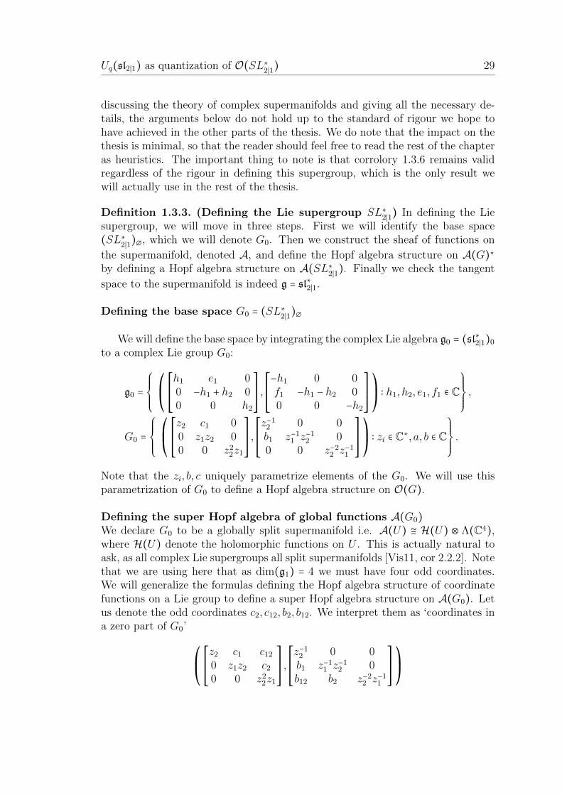
Definition 1.3.3. (Defining the Lie supergroup SL∗2∣1
) In defining the Liesupergroup, we will move in three steps. First we will identify the base space(SL∗
2∣1)∅, which we will denote G0. Then we construct the sheaf of functions on
the supermanifold, denoted A, and define the Hopf algebra structure on A(G)⋆
by defining a Hopf algebra structure on A(SL∗2∣1
). Finally we check the tangent
space to the supermanifold is indeed g = sl∗2∣1.
Defining the base space G0 = (SL∗2∣1
)∅
We will define the base space by integrating the complex Lie algebra g0 = (sl∗2∣1)0
to a complex Lie group G0:
g0 =
⎧⎪⎪⎪⎨⎪⎪⎪⎩
⎛⎜⎝
⎡⎢⎢⎢⎢⎢⎣
h1 e1 00 −h1 + h2 00 0 h2
⎤⎥⎥⎥⎥⎥⎦
,
⎡⎢⎢⎢⎢⎢⎣
−h1 0 0f1 −h1 − h2 00 0 −h2
⎤⎥⎥⎥⎥⎥⎦
⎞⎟⎠∶ h1, h2, e1, f1 ∈ C
⎫⎪⎪⎪⎬⎪⎪⎪⎭
,
G0 =
⎧⎪⎪⎪⎨⎪⎪⎪⎩
⎛⎜⎝
⎡⎢⎢⎢⎢⎢⎣
z2 c1 00 z1z2 00 0 z2
2z1
⎤⎥⎥⎥⎥⎥⎦
,
⎡⎢⎢⎢⎢⎢⎣
z−12 0 0b1 z−1
1 z−12 0
0 0 z−22 z−1
1
⎤⎥⎥⎥⎥⎥⎦
⎞⎟⎠∶ zi ∈ C∗, a, b ∈ C
⎫⎪⎪⎪⎬⎪⎪⎪⎭
.
Note that the zi, b, c uniquely parametrize elements of the G0. We will use thisparametrization of G0 to define a Hopf algebra structure on O(G).
Defining the super Hopf algebra of global functions A(G0)
We declare G0 to be a globally split supermanifold i.e. A(U) ≅ H(U) ⊗ Λ(C4),where H(U) denote the holomorphic functions on U . This is actually natural toask, as all complex Lie supergroups all split supermanifolds [Vis11, cor 2.2.2]. Notethat we are using here that as dim(g1) = 4 we must have four odd coordinates.We will generalize the formulas defining the Hopf algebra structure of coordinatefunctions on a Lie group to define a super Hopf algebra structure on A(G0). Letus denote the odd coordinates c2, c12, b2, b12. We interpret them as ‘coordinates ina zero part of G0’
⎛⎜⎝
⎡⎢⎢⎢⎢⎢⎣
z2 c1 c12
0 z1z2 c2
0 0 z22z1
⎤⎥⎥⎥⎥⎥⎦
,
⎡⎢⎢⎢⎢⎢⎣
z−12 0 0b1 z−1
1 z−12 0
b12 b2 z−22 z−1
1
⎤⎥⎥⎥⎥⎥⎦
⎞⎟⎠

30 Preliminaries on Quantum Supergroups
and use the formulas of 1.1.9 to define the super Hopf algebra structure. Forexample, for the upper triangular part we have
⎡⎢⎢⎢⎢⎢⎣
z2 c1 c12
0 z1z2 c2
0 0 z22z1
⎤⎥⎥⎥⎥⎥⎦
,
⎡⎢⎢⎢⎢⎢⎣
z′2 c′1 c′12
0 z′1z′
2 c′20 0 z
′22 z
′
1
⎤⎥⎥⎥⎥⎥⎦
=
⎡⎢⎢⎢⎢⎢⎣
z2z′2 z2c′1 + c1z′1z′
2 z2c′12 + c1c′2 + c12z′1z′22
0 z1z2z′1z′
2 z1z2c′2 + c2z′1z′22
0 0 z22z1z
′22 z
′
1
⎤⎥⎥⎥⎥⎥⎦
.
We find the following coproduct candidate
∆(z1) = z1 ⊗ z1 ∆(z−11 ) = z−1
1 ⊗ z−11
∆(z2) = z2 ⊗ z2 ∆(z−12 ) = z−1
2 ⊗ z−12
∆(c1) = c1 ⊗ z1z2 + z2 ⊗ c1 ∆(b1) = b1 ⊗ z−12 + z−1
1 z−12 ⊗ b1
∆(c2) = c2 ⊗ z1z22 + z1z2 ⊗ c2 ∆(b2) = b2 ⊗ z
−11 z−1
2 + z−22 z−1
1 ⊗ b2
∆(c12) = c12 ⊗ z1z22 + c1 ⊗ c2 + z2 ⊗ c12 ∆(b12) = b12 ⊗ z
−12 + b2 ⊗ b1 + z
−22 z−1
1 ⊗ b12
where the second row is obtain from a similar calculation on the lower triangularpart. The candidate counit is evaluating the coordinates on the identity element,i.e. ε(zi) = 1, ε(ci) = 0 = ε(bi). Since O(G0) is just a supersymmetric algebra, wecan define ∆(ab) = ∆(a)∆(b) and it is easy to see from the formulas that we havedefined a superbialgebra structure on O(G0).For the antipode we will follow the same strategy, and compute the normal an-tipode, as if we were dealing with normal coordinate functions:
⎡⎢⎢⎢⎢⎢⎣
z2 c1 c12
0 z1z2 c2
0 0 z22z1
⎤⎥⎥⎥⎥⎥⎦
−1
=
⎡⎢⎢⎢⎢⎢⎣
z−12 −c1z−1
1 z−22 −z1z−3
2 (c12 + z−12 c1c2)
0 z−11 z−1
2 −c2z−21 z−3
2
0 0 z−22 z−1
1
⎤⎥⎥⎥⎥⎥⎦
.
We read off the candidate antipode:
S(z1) = z−11 , S(z−1
1 ) = z1,
S(z2) = z−12 , S(z−1
2 ) = z2,
S(c1) = −c1z−11 z−2
2 , S(b1) = −b1z1z22 ,
S(c2) = −z−21 z−3
2 c2, S(b2) = −b2z21z
32 ,
S(c12) = −z−11 z−3
2 (c12 − z−11 z−1
2 c1c2), S(b12) = −z1z32(b12 − z1z2b2b1).
The first thing to note is, that the Hopf algebra maps restricted to the evencoordinates are the same as they would have been coming from 1.1.9 on the Liegroup G0. This is coincidental, because of the triangular form of our matrices.5
Normally one would have to take the Hopf quotient O(G0)/O(G0)1 to obtain the‘usual’ Hopf algebra. Nevertheless, this is a nice bonus as it ensures we have
5We expect that one could have predicted this behaviour by noting that SL∗2∣1 has the structure
of a split Lie supergroup (a group object in the category of split supermanifolds), which is truebecause [(sl∗2∣1)1, (sl
∗2∣1)1] = 0 [Vis11, prop 4.4].

Uq(sl2∣1) as quantization of O(SL∗2∣1
) 31
defined a Hopf algebra structure on the even coordinates. It remains to whetherour S also extends to an antipode for the odd part of the algebra. We check twosuch identities as examples:
µ S ⊗ id ∆(b2) = S(b2)z−11 z−1
2 + z22z1b2
= −b2z32z
21z
−11 z−1
2 + z22z1b2 = 0 = ε(b2),
µ id⊗ S ∆(b12) = b12z2 + b2(−b1z1z22) + z
−22 z−1
1 (−z1z32b12 + z
21z
42b2b1)
= 0 = ε(b12).
As the Hopf structure on the even elements coincides with the usual one, it is veryeasy to give A(G0) a Hopf algebra structure. For fβ where β is some product ofodd coordinates, we can just let ∆(fβ) = ∆usual(f)∆(β).
Sanity check: computing Te(G0,A)We will conclude our description of SL∗
2∣1by computing its tanget Lie superalge-
bra, and showing it is indeed isomorphic to the Lie superalgebra sl∗2∣1. We know
that Te(G0) is spanned by ∂∂b1
∣e, ∂∂c1
∣e, ∂∂z1
∣e, ∂∂z2
∣e, using the exponential map it is
easy to deduce how to translate g0 into this basis.
(H1,−H1) =⎛⎜⎝
⎛⎜⎝
1 0 00 −1 00 0 0
⎞⎟⎠,⎛⎜⎝
−1 0 00 1 00 0 0
⎞⎟⎠
⎞⎟⎠,
et(H1,−H1) =⎛⎜⎝
⎛⎜⎝
et 0 00 e−t 00 0 1
⎞⎟⎠,⎛⎜⎝
e−t 0 00 et 00 0 1
⎞⎟⎠
⎞⎟⎠,
such that
d
dt∣t=0
z1(et(H1,−H1)) =
d
dt∣t=0
e−2t = −2,
d
dt∣t=0
z2(et(H1,−H1)) =
d
dt∣t=0
et = 1,
d
dt∣t=0
c1(et(H1,−H1)) =
d
dt∣t=0
0 = 0,
d
dt∣t=0
b1(et(H1,−H1)) =
d
dt∣t=0
0 = 0.
Of course all odd coordinates vanish on et(H1,−H1). We deduce (H1,−H1) = ( ∂∂z2
− 2 ∂∂z1
) ∣e.We obtain the following correspondence
(H1,−H1) = (∂
∂z2
− 2∂
∂z1
)∣e
, (H2,−H2) =∂
∂z1
∣e
i,
(E1,0) =∂
∂c1
∣e
, (0, F1) =∂
∂b1
∣e
,

32 Preliminaries on Quantum Supergroups
after making the other calculations. TeM has a canonical Lie bracket, from thecoproduct on O(G0). [v, v′](f) = (v ⊗ v′ − v′ ⊗ v)(∆(f)). For completion we willgive a sample calculation to check this indeed gives g0 the structure of (sl∗2∣1)0:
[(H1,−H1), (E1,0)](∆(c1)) = [∂
∂z2
−2∂
∂z1
,∂
∂c1
]e(c1⊗z1z2+z2⊗c1) = 1−(1−2) = 2.
It is easy to see from the coproducts that [(H1,−H1), (E1,0)] will vanish on theother coordinate functions, we conclude [(H1,−H1), (E1,0)] = 2 ∂
∂c1∣e= 2(E1,0).
Recall that Te(G0,A)1 has basis ∂∂b2
∣e, ∂∂b12
∣e, ∂∂c2
∣e, ∂∂c12
∣e
(compare to corrolary
A.2.4.) These odd derivations act as one would expect. For example, ∂∂b2
∣e
only
has non-zero values on functions of the form f(z1, z2, b1, c2)b1, where it has thevalue f(1,1,0,0). In fact, we can just treat these derivations as normal partialderivatives on our function.6 We can use the coproduct again to compute the Liebrackets, for example
[(H1,−H1),∂
∂c2
∣e
] = −∂
∂c2
∣e
, [(H2,−H2),∂
∂c2
∣e
] = 0,
[E1,∂
∂∣e
] = −∂
∂c12
∣e
, [∂
∂c2
∣e
,∂
∂c12
∣e
= 0,
[∂
∂bi∣e
,∂
∂c2
∣e
] = 0,
such that we find that all Lie brackets are compatible with the assignment (E2,0) =∂∂c2
∣e. It is not hard to check that the
(E2,0) =∂
∂c2
∣e
, (0, F2) =∂
∂b2
∣e
,
(E12,0) = [(E2,0), (E1,0)] = −∂
∂c12
∣e
, (0, F12) = [(0, F1), (0, F2)] = −∂
∂b12
∣e
,
assignments yield an isomorphism of Lie superalgebras. We conclude that SL∗2∣1
indeed has sl∗2∣1 as its tangent Lie superalgebra.
Proposition 1.3.4. Let U ′
q be defined as in 1.3.1. We have the following isomor-phism of super Hopf algebras
U1 ≅ O(SL∗2∣1). (1.29)
6To be precise the odd derivations anti-commute with odd coordinate functions, but theseare sent to 0 anyway.

Uq(sl2∣1) as quantization of O(SL∗2∣1
) 33
Proof. Both U ′
1 and O(SL∗2∣1
) are supersymmetric algebras with the same amountof generators, therefore, it suffices to give an algebra isomorphism and checkwhether the other Hopf data (coproduct, antipode, counit) are equal on thesegenerators. The algebra isomorphism is given as follows:
K1 ↦ z1 K2 ↦ z2,
E1 ↦ −c1z−12 F1 ↦ b1z2,
E2 ↦ −c2z−12 z−1
1 F2 ↦ b2z1z2,
E12 ↦ c12z−12 F12 ↦ b12z2.
In order to compare coproducts, we compute the two missing coproducts in U ′
1
∆(F12) = F12 ⊗ 1 + F2K−11 ⊗ F1 +K
−11 K−1
2 ⊗ E12,
∆(E12) = E12 ⊗K1K2 + E1 ⊗ E2K1 + 1⊗ E12.
Indeed, comparing the two coproducts and counits we easily infer that this definesan isomorphism of bialgebras. It remains to check whether the antipodes agree.This can be done by direct calculation, or by noting that antipodes are unique fora bialgebra i.e. an isomorphism of bialgebras must induce an isomorphism of thecorresponding Hopf algebras.
Theorem 1.3.5. O(SL∗2∣1
) is endowed with the structure of a Poisson-Hopf algebrathrough isomorphism 1.3.4. Moreover, SL∗
2∣1is exactly the Poisson-Lie supergroup
integrating sl∗2∣1 with standard Lie bialgebra structure.
Proof. The only thing to check is whether the Poisson bracket indeed induces theright coalgebra structure on sl∗2∣1. We compute the Poisson bracket:
zi, zj = 0, zi, z−
j = 0,
z±i , c1 = ±ai12z±i c1, z±i , c2 = ±
a2i
2z±i c2, z±i , c12 = ±
ai1 + ai22
z±i c12,
z±i , b1 = ∓ai12z±i b1, z±i , c2 = ∓
a2i
2z±i b2, z±i , b12 = ∓
ai1 + ai22
z±i b12,
c1, b1 = z−1i − zi, c1, b2 =
1
2c1b2, c1, b12 = 0,
c2, b1 =1
2c2b1, c2, b2 = z
−12 − z2, c2, b12 = 0,
c12, b1 = 0, c12, b2 = 0, c12, b12 = z1z2 − z−11 z−1
2 ,
c1, c2 = −c12z1z2 c1, c12,= −1
2c1c12, c2, c12 =
1
2c12c2,
b1, b2 = −b12z−12 z−1
1 , b1, b12 = −1
2b12b1, b2, b12 =
1
2b12b2.
We can now compute δ by taking the derivative of the associated Poisson 2-tensorP i.e. P = (z−1
1 − z1)∂∂c1
∧ ∂dellb1
+ . . . . The target space of P is a vector space,

34 Preliminaries on Quantum Supergroups
therefore we can calculate its derivative, by deriving the functions in front of thebasis elements. For example,
δ(E1,0) ∶=d
dt∣t=0
P (et(E1,0)).
Only two terms of P have non-zero derivatives, namely: z1c1∂∂z1
∧ ∂∂c1
− 12z2c1
∂∂z2
∧ ∂∂c1
.
Letting (E1,0), or equivalently ∂∂c1
, act on the functions we find that
δ(E1,0) =∂
∂z1
∧∂
∂c1
−1
2
∂
∂z2
∧∂
∂c1
= −1
2(H1,−H1) ∧ (E1,0) =
1
2(E1,0) ∧ (H1,−H1).
We compute δ(H2,−H2) as final example, leaving the rest to the reader. Recallthat (H2,−H2) = ∂
∂z1∣e. We see that in the Poisson 2-tensor the only non-zero
terms come from the brackets c1, b1 = z−11 − z1 and c12, b12 = z1z2 − z−1
1 z−1. Wecompute:
(H2,−H2)(z−11 − z1) = −2, (H2,−H2)(z1z2 − z
−11 z−1
2 ) = 2
therefore δ(H2,−H2) = −2∂
∂c1
∧∂
∂b1
+ 2∂
∂c12
∧∂
∂b12
= −2(E1,0) ∧ (0, F1) − 2(E12,0) ∧ (0, F12)
which agrees with the cobracket in sl∗2∣1.
Corollary 1.3.6. O((SL∗2∣1
)∅) ∶= O(SL∗2∣1
)/O(SL∗2∣1
)1 has a canonical Poisson-
Hopf structure, which agrees with the Hopf algebra structure on O((SL2∣1)∅) com-ing from proposition 1.1.9.
Proof. This first statement of this corrolary is immediate, by noting that O(SL∗2∣1
)
is a Poisson-Hopf ideal (this is true because both ∆ and , are even). More-over, in this case the structure evens coincides with the Poisson-Hopf structure onO(SL∗
2∣1)0, this is coincidental in this situation. We prove the second statement
by computing the Poisson-Hopf structure O((SL∗2∣1
)∅) = C[b, c, z±1 , z±
2 ], where wedenote b1 and c1 as b resp. c. The Hopf-Poisson structure is given as follows:
zi, zj = 0, zi, z−
j = 0, (1.30)
z±i , c = ±ai12z±i c, c, b = z−1
i − zi, z±i , b = ∓ai12z±i b, (1.31)
and
∆(c) = z2 ⊗ c + c⊗ z1z2, ε(c) = 0, S(c) = −cz−22 z−1
1 , (1.32)
∆(b) = b⊗ z−12 + z−1
1 z−12 ⊗ b, ε(b) = 0, S(b) = −bz2
2z1, (1.33)
∆(zi) = zi ⊗ zi, ε(zi) = 1, S(z±i ) = z∓
i . (1.34)
Chapter 2
Representation Theory of Uε(sl2∣1)
In the early 90s De Concini, Kac and Procesi published a series of papers, amongstothers [DCK90, DCKP92], in which they study quantum groups at roots of unity.We use their methods and ideas to study the quantum supergroup Uq(sl2∣1) at rootsof unity. The algebraic behaviour of a quantum (super)group is very differentat a root of unity then at generic parameter q. Most importantly, one finds thatthe center becomes enlarged, which has profound implications on the representationtheory. In this chapter we reduce the study of the simple representations of Uq(sl2∣1)to studying the representation theory of a family of finite dimensional quotients ofUq(sl2∣1) parametrized by some affine space. Generically these quotients will turnout to be semisimple algebras having `2 different 4`-dimensional simple modulesthat we will concretely describe.
2.1 Structure of the Quantized Universal Envelop-
ing Lie Superalgebra
We begin by studying the structure of Uq(sl2∣1) when we specialize q → ε, whereε ∈ C∗ is a `th primitive root of unity and ` is an odd integer larger than 1. Werecall the definition of Uε(sl2∣1).
Definition 2.1.1. Let Uε denote the quantum supergroup Uε(sl2∣1), defined to bethe C-superalgebra with even generators K±
1 ,K±
2 ,E1, F1 and odd generators E2, F2
subject to the following relations
KiK−1i = 1, KiKj =KjKi, (E0)
KiEj = εaijEjKi, KiFj = ε
−aijFjKi, where A = (2 −1−1 0
) , (E1)
35

36 Representation Theory of Uε(sl2∣1)
EiFj − (−1)ijFjEi = δijKi −K−1
i
ε − ε−1, (E2)
E22 = 0 = F 2
2 , (E3)
E21E2 − (ε + ε−1)E1E2E1 +E2E
21 = 0, (S1)
F 21F2 − (ε + ε−1)F1F2F1 + F2F
21 = 0. (S2)
Lemma 2.1.2. Uε as a super vector space is spanned by monomials
Ks1K
t2E
m1 (E2E1)
oEp2F
m′1 (F2F1)
o′F p′2 (2.1)
where s, t ∈ Z, m,m′ ∈ Z≥0, o, o′, p, p′ ∈ 0,1.
Proof. We will say that a monomial is in standard form if it is of the form as in 2.1.It suffices to show that any monomial reduces to a sum of monomials in standardform. It is easy to see that using equations E0, E1 and E2 we can reduce anymonomial to sums of terms Ks
1Kt2 ∗ e ∗ f with e a monomial in Ei, f a monomial
in Fi. It remains to show we can reduce the e and f parts to sums of monomialsin standard form.
Claim: Any non-zero monomial e in E1 and E2 will have at most 2 E2 terms.Proof claim. Any monomial of the form E2Ea
1E2Eb1E2Ec
1E2 can be reduced to asum of terms of the form E2E1E2E1E2Ed
1 using equation S1. Equation S1 impliesE1E2E1E2 = E2E1E2E1, we deduce that all such terms are equal to E2E2E1E2E1Ed
1 =
0 by E3.
If e contains one E2 term we can use S1 to move any E1 right of E2 to theleft, except possibly one E1. This is covered in the cases o = 0, p = 1 respectivelyo = 1, p = 0. In case e contains two E2 terms we can reduce Ea
1E2Eb1E2Ec
1 to termsof the form Ea
1E2E1E2E1 = Ea1E1E2E1E2. This is covered in the case o = p = 1.
Thus any e can be reduced to a sum of terms in standard form. Reducing f to asum of terms in standard form is analogous.
Of course more is true, the monomials are a basis of Uε. Due to the largeamount of computations involved, we have moved the proof to Appendix B.
Theorem 2.1.3. (PBW Theorem) Uε as a vector space has
Ks1K
t2E
m1 (E12)
oEp2F
m′1 (F12)
o′F p′2 ∶ s, t ∈ Z, m,m′ ∈ Z≥0, o, o
′, p, p′ ∈ 0,1
as a C-linear basis. Here E12 = E2E1 − ε−1E2E1.1
Recall that we Uε endowed with a super Hopf algebra structure in proposition1.1.14.The counit ε ∶ Uε → C, coproduct ∆ ∶ Uε → Uε⊗Uε and antipode S ∶ Uε → Uε
1E12 is known as the quantum commutator, see also example 2.1.6

Structure of the Quantized Universal Enveloping Lie Superalgebra 37
are defined on generators as follows:
∆(Ei) = Ei ⊗Ki + 1⊗Ei, ε(Ei) = 0,
∆(Fi) = Fi ⊗ 1 +K−1i ⊗ Fi, ε(Fi) = 0,
∆(Ki) =Ki ⊗Ki, ε(K±1i ) = 1,
S(Ei) = −EiK−1i ,
S(Fi) = −KiFi,
S(Ki) =K−1i .
Definition 2.1.4. Let Z0 be the subalgebra of Uε generated by E`1, F `
1 , K±`i .
Z0 will turn out to be a central sub-Hopf algebra. In order to show this we willfirst recall some combinatorial identities from quantun calculus, see Appendix E.The quantum (binomial) numbers are defined as follows:
[n] =qn − 1
q − 1, [n]! = [n][n − 1]⋯[1], [
m
n] =
[m]!
[n]![m − n]!.
We set [0]! = 1.Furthermore, we will recall the quantum binomial theorem E.0.49: let x, y beelements in an associative algebra such that yx = q2xy for some scalar q then
(x + y)m =m
∑j=0
[m
j]xjym−j. (QBT)
For q a primitive root of unity, we find that [`] =q`−1q−1 = 0, and hence [
`j] =
[`]⋯[`−j+1][j]! = 0 for 0 < j < `.
Definition 2.1.5. Let σ an automorphism of an associative algebra A. A twistedderivation relative to σ is a linear map D ∶ A→ A such that:
D(ab) =D(a)b + σ(a)D(b).
Example 2.1.6. (i) Any element a ∈ A induces a twisted derivation adσ(a) relativeto σ, defined by adσ(a)(b) = ab − σ(b)a(ii) In Uε we have a natural automorphism, conjugation by K−1
1 : σ(x) =K−11 xK1.
In this case we will suppress σ in the notation of the induced twisted derivationse.g. ad(E1)(E2) will be understood to mean adσ(E1)(E2).
The twisted derivation of Uε will allow us to replace the Serre type relationsS1 and S2 by ones using ad:
ad(E1)2(E2) = ad(E1)(E1E2 −K
−11 E2K1E1)
= E21E2 −K1E1E2K
−11 E1 − εE1E2E1 + εK1E2E1K
−11 E1
= E21E2 − (ε−1 + ε)E1E2E1 +E2E
21 ,

38 Representation Theory of Uε(sl2∣1)
and similarly ad(F1)2(F2) = F 2
1F2 − (ε + ε−1)F1F2F1 + F2F 21 .
In this notation we have
E12 = −q−1ad(E1)(E2), F12 = ad(F1)(F2).
Proposition 2.1.7. Let σ be an automorphism of some associative algebra A,a ∈ A s.t. σ(a) = q2a, define adσ(a)(b) = ab − σ(b)a. The identity
adσ(a)m(b) =
m
∑j=0
(−1)jqj(j−1)[m
j]am−jσj(b)aj
holds in A for all a, b ∈ A.
Proof. Let La,Ra ∈ End(A) denote the left and right multiplication with a respec-tively. We can write
ada = La −Raσ
Since A is associative La and Ra commute, we find that
La(Raσ)(b) = aσ(b)a = q−2σ(a)σ(b)a = q−2(Raσ)La(b)
holds for all a, b ∈ A. Thus we are in the position to apply lemma QBT to La,Raσ ∈
End(A):
(adσ(a))m = (La −Raσ)
m =m
∑j=0
(−1)j[m
j]Lm−ja (Raσ)
j.
As σRa = q2Raσ we find, using a simple induction argument, that (Raσ)j =
qj(j−1)Rjaσj. This completes the computation.
Corollary 2.1.8. Let ε ∈ C be a primitve `th root of unity, A an associative algebrawith automorphism σ s.t. σ(a) = ε2a for some a ∈ A. Then
(adσa)`(b) = a`x − σ`(x)al.
Proof. This follows directly from applying the QBT.
Proposition 2.1.9. Z0 is a central Hopf subalgebra of Uε, with Hopf maps definedon generators as follows
∆(E`1) = E
`1 ⊗K
`1 + 1⊗E`
1, S(E`1) = −E
`1K
`1, ε(E`
1) = 0,
∆(F `1) = F
`1 ⊗ 1 +K−`
1 ⊗ F `1 , S(F `
1) = −Fl1K
−`1 , ε(F `
1) = 0,
∆(K±`1 ) =K±`
1 ⊗K±`1 , S(K±`
1 ) =K∓`1 , ε(K±`
1 ) = 1.
Proof. Recall that Z0 is the subalgebra generated by E`1, F
`1 ,K
±`1 ,K
±`2 . To show Z0
is central it suffices to check that the generators of Z0 commute with the generatorsof Uε. As ε` = 1 obviously K±`
1 and K±`2 are central. We will show that E`
1 is central

Structure of the Quantized Universal Enveloping Lie Superalgebra 39
and leave out the computations for F `1 as they are completely analogous.
The commutator with Ki can be computed directly:
E`1Ki = ε
−ai1E`−11 K1E1 = ε
−`ai1K1E`1 =K1E
`1.
For [E`1,E2] we use corollary 2.1.8 with σ conjugation byK1. Recall that ad(E1)
2E2 =
0 is exactly our Serre type relation. Therefore,
0 = ad(E1)`(E2) = E
`1E2 − σ
`(E2)El1 = E
`1E2 − ε
`a12E2E`1 = E
`1E2 −E2E
`1
holds. Since E1 commutes with F2, so does El1. It remains to compute the com-
mutator of El1 with F1. We will make use of a telescopic expansion:
[E`1, F1] = E
`−11 E1F1 −E
`−11 F1E1 +E
`−21 E1F1E1 −E
`−21 F1E1E1 + . . .
⋅ ⋅ ⋅ +E1F1E`−11 − F1E1E
`−11
= E`−11
K1 −K−11
ε − ε−1+E`−2
1
K1 −K−11
ε − ε−1E1 + ⋅ ⋅ ⋅ +
K1 −K−11
ε − ε−1E`−1
1
=E`−1
1 K1
ε − ε−1
`−1
∑i=0
ε2i +E`−1
1 K−11
ε − ε−1
`−1
∑j=0
ε−2j
=E`−1
1 K1
ε − ε−1
1 − ε2`
1 − ε2+E`−1
1 K−11
ε − ε−1
1 − ε−2`
1 − ε−2
= 0.
Thus Z0 is indeed central. It remains to show it is a Hopf subalgebra. For thitsuffices to check Z0 is closed under the coproduct and antipode. Since Z0 is asubalgebra it suffices to check that Z0 is closed under coproduct and antipode onthe generators. We first check the generators K±
i :
∆(K±`i ) = ∆(Ki)
±` = (Ki ⊗Ki)±` =K±`
i ⊗K±`i ∈ Z0 ⊗Z0,
S(K±`i ) = S(Ki)
` =K∓`i ∈ Z0.
Note that in the above we are using that ∆ and S are an algebra homorphism andanti-homomorphism respectively. For E1 we have coproduct ∆(E1) = E1 ⊗K1 +
1⊗E1. As E1⊗K1 ⋅1⊗E1 = q21⊗E1 ⋅E1⊗K1, we can use lemma QBT to computethat
∆(E`1) = ∆(E1)
` = (E1 ⊗K1 + 1⊗E1)` = E`
1 ⊗K`1 + 1⊗E`
1 ∈ Z0 ⊗Z0.
The antipode can be calculated directly:
S(E`1) = S(E1)
` = (−E1K1)` = (−1)`E`
1K`1ε
−(0+2+⋅⋅⋅+2(`−1)
= −E`1K
`1ε
−`(`−1) = −E`1K
`1 ∈ Z0.
We leave the computation for F `1 .
Corollary 2.1.10. Uε is a free Z0 module of dimension 16`4.
Proof. This is immediate from the PBW-theorem 2.1.3.

40 Representation Theory of Uε(sl2∣1)
2.2 Generic representations of Uε(sl2)
We will describe a family of modules of Uε(sl2) dependent on three variables inC2 ×C∗. Generically, i.e. in a dense subset of C2 ×C∗, these modules are simpleUε(sl2)-modules.
The algebra Uε(sl2) is defined to be the subalgebra of Uε(sl2∣1) generated by E1, F1
and K1.
Convention. We will often drop the subindices 1 when describing elements inUq(sl2) e.g. we will write K rather than K1.
The structure of generic simple representations of Uε(sl2) is well known. Seefor example [BG02a, §III].
Lemma 2.2.1. [BG02a, Th. III.2.2] Let λ ∈ C∗, a, b ∈ C, and let V be a complexvector space with basis m0, . . . ,ml−1. The following action makes V into a simpleUε(sl2)-module, denoted V (a, b, λ).
Kmi = λε−2imi
Fmi =
⎧⎪⎪⎨⎪⎪⎩
mi+1 if i < ` − 1
bm0 if i = ` − 1
Emi =
⎧⎪⎪⎨⎪⎪⎩
am`−1 ∶= e0m`−1 if i = 0
(ab + (εi−ε−i)(λε1−i−λ−1εi−1)(ε−ε−1)2 mi−1 ∶= eimi−1 if i > 0
If λ ≠ ±εi for any i ∈ Z or b ≠ 0, then V (a, b, λ) is a simple Uε(sl2)-module.
Remark. The ei introduced above are useful abbreviations of which we will makeuse to shorten some of the long expressions.
Proposition 2.2.2. Let V (a, b, λ) be a simple U(sl2)-module as described above.For 1 ≤ i ≤ l − 1 we have
V (a, b, λ) ≅ V (eib−1, b, λε−2i)
as U(sl2)-modules
Proof. Let the linear map V (a, b, λ)→ V (eib−1, b, λε−2i) be given on the basis as
mj ↦
⎧⎪⎪⎪⎪⎪⎪⎪⎨⎪⎪⎪⎪⎪⎪⎪⎩
m`−1b if j = i − 1
bml−1−i if j = ` − 1
mj−i if j − i ≥ 0, j ≠ ` − 1
ml+j−i otherwise
It is now an easy calculation to check that the Uε(sl2) action commutes with thismap.
We will call the simple modules V (a, b, λ) the generic representations of Uε(sl2).This terminology will be explained in the final section of this chapter.

Generic Representations of Uε(sl2∣1) 41
2.3 Generic Representations of Uε(sl2∣1)
As we have Uε(sl2) ⊂ Uε(sl2∣1) it is natural to ask whether we can extend the (sim-ple) generic Uε(sl2)-modules to simple Uε(sl2∣1)-module. Let Uε(sl2) ⊗ C[K±
2 ] ≅
U evenε be the even part of Uε. Given λ2 ∈ C∗, each simple Uε(sl2)-module V (a, b, λ1)
extends naturally to a simple U evenε -module V (a, b, λ1, λ2) by lettingK2mi = λ2εimi.
The following proposition describes simple Uε(sl2∣1)-modules naturally extendingthe generic U even
ε -modules.
Theorem 2.3.1. Let V = V (a, b, λ1, λ2), be a simple U evenε -module. We define
super vector space
W (a, b, λ1, λ2) ∶= V ⊕E2V ⊕E12V ⊕E12E2V
i.e. a (2`,2`)-dimensional vector space, denoted shortly W , with even resp. oddbasis
mi,E2E1E2mi0≤i≤`−1 ∪ E2mi,E1E2mi0≤i≤`−1
The following action endows W with an Uε-module structure.
K1 ⋅mi = λ1ε−2i K2 ⋅mi = λ2ε
i,
K1 ⋅E2mi = λ1ε−2i−1 K2 ⋅E2mi = λ2ε
i,
K1 ⋅E1E2mi = λ1ε−2i+1 K2 ⋅E1E2mi = λ2ε
i−1,
K1 ⋅E2E1E2mi = λ1ε−2i K2 ⋅E2E1E2mi = λ2ε
i−1,
E1 ⋅mi = eimi−1,
E1 ⋅E2mi = E1E2mi,
E1 ⋅E1E2mi = (ε + ε−1)eiE1E2mi−1 − eiei−1E2mi−2,
E1 ⋅E2E1E2mi = eiE2E1E2mi−1,
E2 ⋅mi = E2mi,
E2 ⋅E2mi = 0,
E2 ⋅E1E2mi = E2E1E2mi,
E2 ⋅E2E1E2mi = 0,

42 Representation Theory of Uε(sl2∣1)
F1 ⋅mi =
⎧⎪⎪⎨⎪⎪⎩
mi+1 if i < l − 1
bm0 if i = l − 1,
F1 ⋅E2mi =
⎧⎪⎪⎨⎪⎪⎩
E2mi+1 if i < l − 1
bE2m0 if i = l − 1,
F1 ⋅E1E2mi =
⎧⎪⎪⎨⎪⎪⎩
E1E2mi+1 −λ1ε
−2i−1−λ−11 ε2i+1
ε−ε−1 E2mi if i < l − 1
bE1E2m0 −λ1ε−λ
−11 ε−1
ε−ε−1 E2ml−1 if i = l − 1,
F1 ⋅E2E1E2mi =
⎧⎪⎪⎨⎪⎪⎩
E2E1E2mi+1 if i < l − 1
bE2E1E2m0 if i = l − 1,
F2 ⋅mi = 0,
F2 ⋅E2mi =λ2εi − λ−1
2 ε−i
ε − ε−1mi,
F2 ⋅E1E2mi = eiλ2εi − λ−1
2 ε−i
ε − ε−1mi−1,
F2 ⋅E2E1E2mi =λ2εi−1 − λ−1
2 ε1−i
ε − ε−1E1E2mi − ei
λ2εi − λ−12 ε
−i
ε − ε−1E2mi−1,
Moreover, W (a, b, λ1, λ2) is simple when
(λ2λ1 − λ−12 λ
−11 )(λ2ε
−1 − λ−12 ε
) + ab(2 − ε2 − ε−2) ≠ 0,
and V (a, b, λ1, λ2) is simple i.e. λ1 ≠ ±εi for i ∈ Z or b ≠ 0.
Proof. Showing that the action defines a module structure on W boils down tochecking whether the defining relations E0−E3, S1, S2 of Uε are respected by themodule structure. These are easy but sometimes lenghthy calculations. We check
the relation E2F2 + F2E2 =K2−K
−12
ε−ε−1 as example:
(E2F2 + F2E2) ⋅mi = F2 ⋅E2mi
=λ2εi − λ2ε−i
ε − ε−1mi =
K2 −K−12
ε − ε−1mi,
(E2F2 + F2E2) ⋅E2mi = E2 ⋅λ2εi − λ2ε−i
ε − ε−1mi
=K2 −K−1
2
ε − ε−1E2mi,

Generic Representations of Uε(sl2∣1) 43
(E2F2 + F2E2) ⋅E1E2mi = E2 ⋅ (eiλ2εi − λ−1
2 ε−i
ε − ε−1mi−1)
+λ2εi−1 − λ−1
2 ε1−i
ε − ε−1E1E2mi − ei
λ2εi − λ−12 ε
−i
ε − ε−1E2mi−1
=K2 −K−1
2
ε − ε−1E1E2mi,
(E2F2 + F2E2) ⋅E2E1E2mi = E2 ⋅ (λ2ε1−i − λ−1
2 εi−1
ε − ε−1E1E2mi
− eiλ2ε−i − λ−1
2 εi
ε − ε−1E2mi−1) =
λ2ε1−i − λ−12 ε
i−1
ε − ε−1E2E1E2mi
=K2 −K−1
2
ε − ε−1E2E1E2mi,
Finally we show that W is simple for the given conditions. Let M ≠ 0 be asubmodule of W . Since ε is primitive root of unity we find that W is the sum ofits distinct Ki eigenspaces Wm,n ∶= w ∈W ∶K1w = λ1εmw,K2w = λ2εnw
W =∑i
W−2i,i ⊕W−2i−1,i ⊕W−2i+1,i−1 ⊕W−2i,i−1
=∑i
Cmi ⊕CE2mi ⊕CE1E2mi ⊕CE2E1E2mi
There is degeneracy for W−2i−1,i and W−2i−1,i+1. Nevertheless W , and therefore alsoM , are spanned by the eigenvectors it contains.Since M ≠ 0 it contains at least one such eigenvector. Suppose mi ∈M , then by theUε(sl2) action V ⊂M (note we use here that W extends the simple Uε(sl2)-moduleV (a, b, λ1)). The E1 and E2 action then yield M = W . If E2mi + αE1E2mi+1 ∈
M , we have E2E1E2mi ∈ M (which is also the last case). A straightforwardcomputation, which we leave out due to its length, yields
F2F1F2 ⋅E2E1E2mi =(λ2λ1 − λ−1
2 λ−11 )(λ2ε−1 − λ−1
2 ε) + ab(2 − ε2 − ε−2)
(ε − ε−1)2mi
which is a non-zero multiple of mi by assumption. Therefore, in all cases we reduceto the case mi ∈M which implies M =W .
Proposition 2.3.2. We find the following isomorphisms between the modules de-scribed in theorem 2.3.1:
W (a, b, λ1, λ2) ≅W (eib−1, b, ε−2iλ1, ε
iλ2)
for i ∈ 1, . . . , l − 1.
Proof. An easy corrolary to proposition 2.2.2.

44 Representation Theory of Uε(sl2∣1)
2.4 Sets of irreducible representations parametrized
over the dual Poisson Lie group
In this section we show that Z0, as a Hopf algebra, can be seen as the coordinatering on the even part of the dual Poisson Lie supergroup of SL2∣1. Furthermore, wecan identify maxSpec(Z0) = (SL∗
2∣1)∅. We define a family of algebras over (SL∗
2∣1)∅
and use it to analyze the representation theory of Uε.
Recall that the even part of the dual Poisson Lie group is defined as follows
(SL∗2∣1)∅ = ⎛⎜⎝
⎡⎢⎢⎢⎢⎢⎣
∗ ∗ 00 ∗ 00 0 ∗
⎤⎥⎥⎥⎥⎥⎦
,
⎡⎢⎢⎢⎢⎢⎣
∗ 0 0∗ ∗ 00 0 ∗
⎤⎥⎥⎥⎥⎥⎦
⎞⎟⎠∈ SL2∣1 × SL2∣1 ∶ inv. diag. elements .
We write Ω for short, and use the parametrization
⎛⎜⎝
z2 c 00 z1z2 00 0 z2
2z1
⎞⎟⎠,⎛⎜⎝
z−12 0 0b z−1
1 z−12 0
0 0 z−22 z−1
1
⎞⎟⎠∶ zi ∈ C∗, a, b ∈ C
to identify Ω as a set with a quasi-affine variety in C4. Denote O(Ω) the ring of(regular or algebraic) functions on Ω, we have that O(Ω) = C[b, c, z1, z2, z−1
1 , z−12 ] =
C[b, c, z1, z2]z1,z2 .
Lemma 2.4.1. O(Ω) is a Hopf-algebra with Hopf maps defined on the genetorsof O(Ω) as:
∆(c) = z2 ⊗ c + c⊗ z1z2, ε(c) = 0, S(c) = −cz−22 z−1
1
∆(b) = b⊗ z−12 + z−1
1 z−12 ⊗ b, ε(b) = 0, S(b) = −bz2
2z1
∆(zi) = zi ⊗ zi, ε(zi) = 1, S(z±i ) = z∓
i
Proof. We can use proposition 1.1.9, or equivalently corrolary 1.3.6.
Proposition 2.4.2. We have an isomorphism of Hopf algebras
Z0 → O(Ω),
− (ε − ε−1)`E`1 ↦ cz−1
2 , (ε − ε−1)F `1 ↦ bz2, K±`
i ↦ z±i .
Proof. Why we chose these specific coefficients for E`1 and F `
1 will become clearin the next chapter. Obviously this is an isomorphism of commutative algebras.Therefore, it suffices to check that the Hopf-algebra structure on Z0 in proposition2.1.9 is respected by the map, denote it φ, on generators. This is trivial for z1, z2
and the counit. It remains to check coproduct and antipode on E`1 and F `
1 , to

Sets of representations parametrized over (SL∗2∣1
)∅ 45
improve readability we leave out the coefficients (ε − ε−1)` in the computations:
∆(φ(E`1)) = ∆(cz−1
2 ) = ∆(c)∆(z−12 ) = (z2 ⊗ c + c⊗ z1z2)z
−12 ⊗ z−1
2
= cz−12 ⊗ z1 + 1⊗ cz−1
2 = φ(∆(E`1),
S(φ(E`1)) = S(cz
−12 ) = −cz−2
2 z−11 = φ(−E`
1)φ(K−`1 ) = φ(S(E`
1)),
∆(φ(F `1)) = ∆(bz2) = ∆(b)∆(z2) = (z−1
2 z−11 ⊗ b + b⊗ z−1
2 )z2 ⊗ z2
= bz2 ⊗ 1 + z−11 ⊗ cz2 = φ(∆(F `
1),
S(φ(F `1)) = S(bz2) = −bz
22z1 = φ(−F
`1)φ(K
l1) = φ(S(F
`1)).
Recall the definition of the spectrum of a ring, in the sense of [DCP93].
Definition 2.4.3. Let A be a unital algebra algebra over C. We define mSpec(A)
to be the set of all equivalence classes of finite dimensional simple representationsover C.
We have the following variation of Schur’s lemma.
Lemma 2.4.4. (Schur’s lemma) Let A be an associative unital algebra of countabledimension that is finitely generated over its center Z. For a simple representationV we have:1. dim(V ) <∞.2. Hom(V,V ) = C ⋅ id.
Proof. We will prove the statements in reverse order. Denote Z(V ) ∶= f ∈
Hom(V,V ) ∶ ∃z ∈ Z s.t. f(a) = z ⋅ a ∀a ∈ A. Let a1, . . . , an generate A asa Z-module. As V is simple A ⋅ v = V for any v ≠ 0. For such a v we have thata1 ⋅ v, . . . , an ⋅ v generate V as a Z(V )-module. Thus V is finitely generated asZ(V )-module. For 0 ≠ f ∈ Z(V ) we find that f(V ) = V since x ⋅f(v) = f(x ⋅v) im-plies f(V ) is a proper submodule of the simple module V . By Nakayama’s lemmathere must exist a g ∈ Z(V ) s.t. (1 − fg)V = 0 i.e. f is invertible. Then Z(V ) isa field over C, and hence equals C by lemma D.0.41. This concludes the proof oftwo. One follows immediately as V is finitely generated over Z(V ) = C.
We can now connect mSpec(A) to the usual definition in algebraic geometry,and hence endow mSpec(A) with a Zariski topology.
Lemma 2.4.5. Let A = [x1, . . . , xn, y1, y−11 , . . . , ym, y−1
m ], then mSpec(A) can beidentified with the maximal spectrum of A in the sense of D.0.38.
Proof. Note that A satisfies the conditions of Schur’s lemma. All xi, yi are centraland hence must act as scalars on simple representations. The one dimensionalsimple representations are thus completely characterized by the values of the xiand yi. The generalized weak Nullstellensatz D.0.43 tells us that exactly describesthe maximal ideals of A i.e. the closed points in Spec(A).
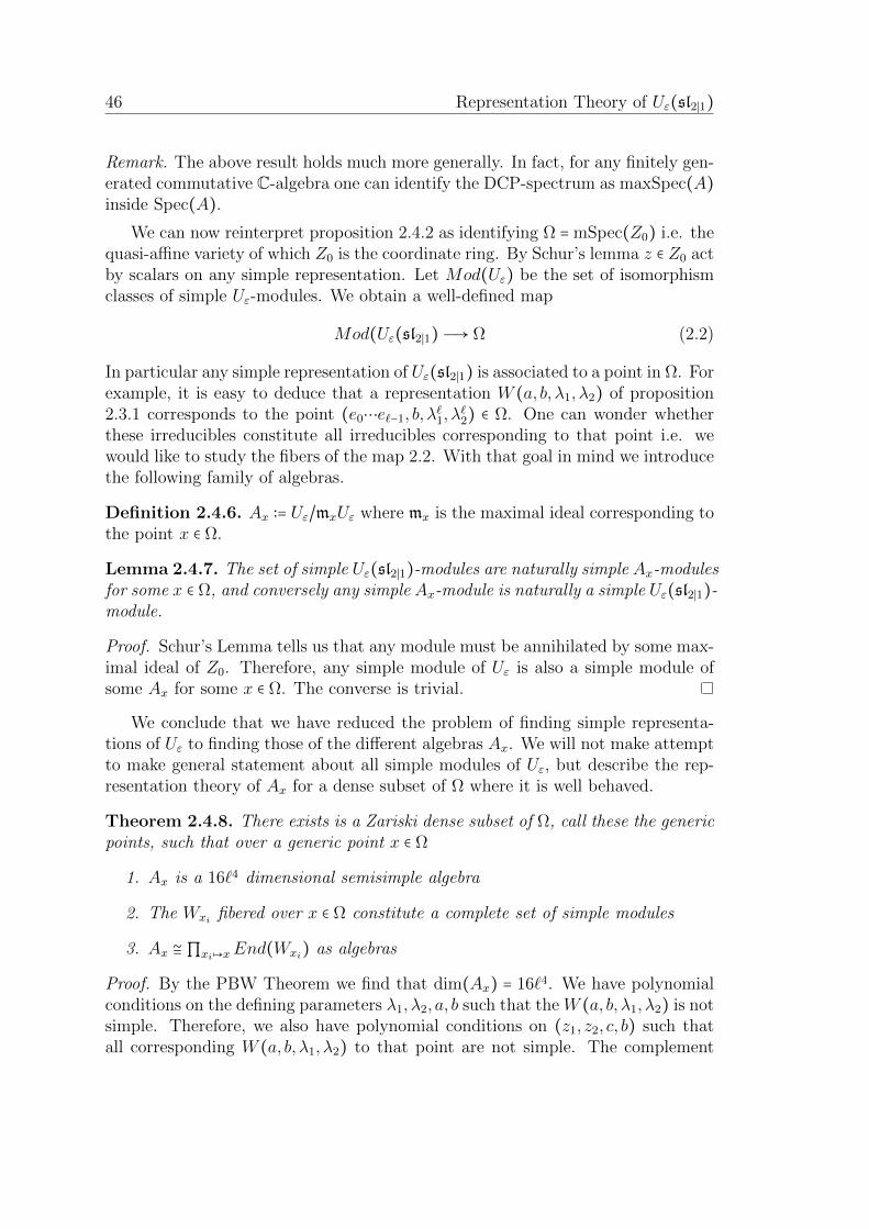
46 Representation Theory of Uε(sl2∣1)
Remark. The above result holds much more generally. In fact, for any finitely gen-erated commutative C-algebra one can identify the DCP-spectrum as maxSpec(A)
inside Spec(A).
We can now reinterpret proposition 2.4.2 as identifying Ω = mSpec(Z0) i.e. thequasi-affine variety of which Z0 is the coordinate ring. By Schur’s lemma z ∈ Z0 actby scalars on any simple representation. Let Mod(Uε) be the set of isomorphismclasses of simple Uε-modules. We obtain a well-defined map
Mod(Uε(sl2∣1)Ð→ Ω (2.2)
In particular any simple representation of Uε(sl2∣1) is associated to a point in Ω. Forexample, it is easy to deduce that a representation W (a, b, λ1, λ2) of proposition2.3.1 corresponds to the point (e0⋯e`−1, b, λ`1, λ
`2) ∈ Ω. One can wonder whether
these irreducibles constitute all irreducibles corresponding to that point i.e. wewould like to study the fibers of the map 2.2. With that goal in mind we introducethe following family of algebras.
Definition 2.4.6. Ax ∶= Uε/mxUε where mx is the maximal ideal corresponding tothe point x ∈ Ω.
Lemma 2.4.7. The set of simple Uε(sl2∣1)-modules are naturally simple Ax-modulesfor some x ∈ Ω, and conversely any simple Ax-module is naturally a simple Uε(sl2∣1)-module.
Proof. Schur’s Lemma tells us that any module must be annihilated by some max-imal ideal of Z0. Therefore, any simple module of Uε is also a simple module ofsome Ax for some x ∈ Ω. The converse is trivial.
We conclude that we have reduced the problem of finding simple representa-tions of Uε to finding those of the different algebras Ax. We will not make attemptto make general statement about all simple modules of Uε, but describe the rep-resentation theory of Ax for a dense subset of Ω where it is well behaved.
Theorem 2.4.8. There exists is a Zariski dense subset of Ω, call these the genericpoints, such that over a generic point x ∈ Ω
1. Ax is a 16`4 dimensional semisimple algebra
2. The Wxi fibered over x ∈ Ω constitute a complete set of simple modules
3. Ax ≅∏xi↦xEnd(Wxi) as algebras
Proof. By the PBW Theorem we find that dim(Ax) = 16`4. We have polynomialconditions on the defining parameters λ1, λ2, a, b such that the W (a, b, λ1, λ2) is notsimple. Therefore, we also have polynomial conditions on (z1, z2, c, b) such thatall corresponding W (a, b, λ1, λ2) to that point are not simple. The complement

Sets of representations parametrized over (SL∗2∣1
)∅ 47
defines some Zariski open set in Ω. We find we have `2 different 4` dimensionalsimple modules W (a, b, λ1, λ2) of Ax. To be precise, we find that we have `3
corresponding choices of (a, b, λ1, λ2) corresponding to a point (c, b, z1, z2), butproposition 2.3.2 tells us we have counted ` times to many modules. It is easy tosee that the remaining modules are all non-isomorphic. We count dimensions andapply Corrolary C.0.37.
Remark. Now we are finally in a position to truly appreciate the name ‘genericsimple module’. If we randomly pick a simple Uε(sl2∣1)-module, generically (withpropability one) we will pick one of the generic simple modules in theorem 2.4.8.
Corollary 2.4.9. Generically the map
Mod(Uε)→ Ω
is `2 to 1.
Proof. By Schur’s Lemma we know that every simple module lies over a point inx ∈ Ω, and hence can be interpreted as a simple module of Ax. From the previousproposition we see that for a generic point the fiber contains `2 different simplemodules.


Chapter 3
The Quantum Coadjoint Action
Recall that (SL∗2∣1
)∅ has a canonical Poisson-Hopf structure induced from Uε. Weshow that Z0 has a canonical Poisson-Hopf structure as well and prove the isomor-phism of theorem 2.4.2 is in fact an isomorphism of Poisson-Hopf algebras. Wethen construct an action of an infinite dimensional group on Ω whose orbits areprecisely the symplectic leaves. Finally we show that Ax can be seen as the fibersof a smooth vector bundle over the symplectic leaves whose fibers are isomorphicas algebras.
3.1 A canonical Poisson structure on Z0
Let us recall how we defined the Poisson structure on O(SL∗2∣1
): we had a familyof algebras deforming the function algebra and dequantized the deformation toget a Poisson structure on O(SL∗
2∣1). In similar spirit one can think that we
have a family of non-commutative Z0∣q deforming the commutative Z0∣q=ε. Thisis exactly how we will define a Poisson bracket for Z0, although we will choosea useful normalization. First, however, we will introduce an alternative type ofquantum numbers and prove a small lemma that we will need in working withthem.
Definition 3.1.1. (Alternative Quantum Numbers) When trying to find generalformulae for commuting powers of the generators in Uq(sl2∣1) quantum numbersnaturally appear. The most natural, or useful, ones in this case are closely relatedto, but slightly different from, the ones we defined in the appendix. For n ∈ N
49
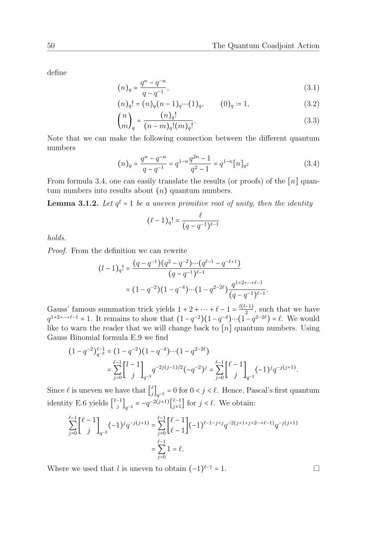
50 The Quantum Coadjoint Action
define
(n)q =qn − q−n
q − q−1, (3.1)
(n)q! = (n)q(n − 1)q⋯(1)q, (0)q ∶= 1, (3.2)
(n
m)q
=(n)q!
(n −m)q!(m)q!. (3.3)
Note that we can make the following connection between the different quantumnumbers
(n)q =qn − q−n
q − q−1= q1−n q
2n − 1
q2 − 1= q1−n[n]q2 (3.4)
From formula 3.4, one can easily translate the results (or proofs) of the [n] quan-tum numbers into results about (n) quantum numbers.
Lemma 3.1.2. Let q` = 1 be a uneven primitive root of unity, then the identity
(` − 1)q! =`
(q − q−1)`−1
holds.
Proof. From the definition we can rewrite
(l − 1)q! =(q − q−1)(q2 − q−2)⋯(q`−1 − q−`+1)
(q − q−1)`−1
= (1 − q−2)(1 − q−4)⋯(1 − q2−2`)q1+2+⋅⋅⋅+`−1
(q − q−1)`−1.
Gauss’ famous summation trick yields 1 + 2 + ⋅ ⋅ ⋅ + ` − 1 =l(l−1)
2 , such that we haveq1+2+⋅⋅⋅+`−1 = 1. It remains to show that (1− q−2)(1− q−4)⋯(1− q2−2`) = `. We wouldlike to warn the reader that we will change back to [n] quantum numbers. UsingGauss Binomial formula E.9 we find
(1 − q−2)`−1q−2 = (1 − q−2)(1 − q−4)⋯(1 − q2−2`)
=`−1
∑j=0
[l − 1
j]q−2q−2j(j−1)/2(−q−2)j =
`−1
∑j=0
[` − 1
j]q−2
(−1)jq−j(j+1).
Since ` is uneven we have that [`j]q−2
= 0 for 0 < j < `. Hence, Pascal’s first quantum
identity E.6 yields [`−1j]q−2
= −q−2(j+1)[`−1j+1
] for j < `. We obtain:
`−1
∑j=0
[` − 1
j]q−2
(−1)jq−j(j+1) =`−1
∑j=0
[` − 1
` − 1](−1)`−1−j+jq−2(j+1+j+2⋅⋅⋅+`−1)q−j(j+1)
=`−1
∑j=0
1 = `.
Where we used that l is uneven to obtain (−1)`−1 = 1.

A canonical Poisson structure on Z0 51
Proposition 3.1.3. Z0 has a canonical Poisson structure by letting
a, b = limq→ε
ab − ba
`(q` − q−`)(3.5)
Proof. Note that if ε is a primitive root of unity with ` ≥ 3, then q`−q−` as a functionof q has a zero of order 1 in ε. Thus we are just renormalizing the definition ofthe Poisson structure in proposition 1.2.3. Hence the result is immediate if thedeformation of Z0 by the family Z0 is nice (smooth) enough around ε. We willshow this by explicitly computing the Poisson structure.
To compute the Poisson structure of Z0 we will need a useful identity due toKac
Lemma 3.1.4. For simplicity denote E = E1, F = F1, K = K1 in Uq(sl2∣1), thefollowing identity holds
[Em, F s] =
min(m,s)
∑j=1
(m
j)q
(s
j)q
(j)q!Fs−j
2j−m−s
∏r=j+1−m−s
[K; r]Em−j (3.6)
where [K; r] ∶= Kqr−K−1q−rq−q−1 .
Proof. We will prove this formula, by a rather elaborate double induction. We willdrop the qs in the notation of the binomials and factorials to improve readability.
For m = 1, s = 1 [E,F ] =K −K−1
q − q−1=
1
∑j=1
(1
1)(
1
1)(1)!F 0
0
∏r=0
[K; 0]E0
Now suppose the formula holds for m = 1, s, we find that
[E,F s+1] = F [E,F s] + [E,F ]F s = F (s)F s−1[K; 1 − s] + [K; 0]F s
= F s([K; 1 − s](s) + [K;−2s])
= F sKq−s(q(s) + q−s(1)) −K−1qs(q(s) + qs(1)
q − q−1
= (s + 1)F s[K; s].
We used that qj(i) + qi(j) = (i + j) and [K; i]F j = F j[K; i − 2j].

52 The Quantum Coadjoint Action
Now suppose the formula holds for m,s, we find that:
[Em+1, F s] = E[Em, F s] + [E,F s]Em
= Emin(m,s)
∑j=1
(m
j)(s
j)(j)!F s−j
2j−m−s
∏r=j+1−m−s
[K; r]Em−j + (s)F s−1[K; 1 − s]Em
now use [E,F s−j] = (s − j)F s−j−1[K; 1 − (s − j)]
=
min(m,s)
∑j=1
(m
j)(s
j)(j)!(s − j)F s−j−1[K; 1 − s + j]
2j−m−s
∏r=j+1−m−s
[K; r]Em−j+
+
min(m,s)
∑j=1
(m
j)(s
j)(j)!F s−j
2j−m−s
∏r=j+1−m−s
[K; r − 2]Em−j+1 + (s)F s−1[K; 1 − s]Em
=
min(m,s)+1
∑j=2
(m
j − 1)(s
j)(j)!F s−j−1[K; j − s]
2(j−1)−m−s
∏r=j+1−(m+1)−s
[K; r]Em+1−j+ (*)
+
min(m,s)
∑j=2
(m
j)(s
j)(j)!F s−j
2(j−1)−m−s
∏r=j+1−(m+1)−s−1
[K; r]Em+1−j (*)
+ (m)(s)F s−1[K;−m − s]Em + (s)F s−1[K; 1 − s]Em (**)
where we used (sj−1
)(j − 1)!(s − j + 1) = (sj)(j)! in the last line. We now wish to
merge the two large sums from j = 2 up to j =min(m,s) in the lines (*). Note thatthe second sum has an extra term in the product for r = j + 1 − (m + 1) − s − s − 1.We compute:
(m
j − 1)[K; s − j] + (
m
j)[K; j −m − s − 1]
= (m + 1
j)
1
(m + 1)((j)[K; s − j] + (m − j + 1)[K; j −m − s − 1])
= (m + 1
j)[K; 2j − (m + 1) − s].
This exactly yields the following expression
min(m,s)
∑j=2
(m + 1
j)(s
j)(j)!F s−j−1[K; j − s]
2j−(m+1)−s
∏r=j+1−(m+1)−s
[K; r]Em+1−j.
For the j = 1 term we add the two terms of line (**):
(m)(s)F s−1[K;−m − s]Em + (s)F s−1[K; 1 − s]Em
= (m + 1
1)(s
1)(1)!F s−1[K; 2 − (m + 1) − s]Em.
This is exactly the j = 1 term in the right hand side of 3.6 for m + 1.Finally we need to match our min(m,s)+1 term in (*), with the j =min(m+1, s)

A canonical Poisson structure on Z0 53
term in the right hand side of 3.6. Denote n = min(m + 1, s) and n′ = min(m,s),we wish to check whether
(m
n)(s
n)(n)!(s − n)F s−n[K; 1 − s − n]
2n−m−s
∏r=n+1−m+s
[K; r]Em−n
?=
min(m+1,s)
∑n′=min(m,s)+1
(m + 1
n′)(s
n′)(minn′)!F s−n′[K; 1 − s − n′]
2n′−(m+1)−s
∏r=n′+1−(m+1)+s
[K; r]Em+1−n′
holds. If s < m the LHS is 0, as (s − j + 1) = (0) = 0. This equals the RHS,since min(m + 1, s) = min(m,s) = s implies it is an empty sum. If m < s we havemin(m,s) + 1 = m + 1 = min(m + 1, s), we need to match the seperate parts ofthe expression: (
mm) = (
m+1m+1
), we again write (sj−1
)(j − 1)!(s − j + 1) = (sj)(j)! and
[K; j − s] = [K;m + 1 − s] = [K; 2(m + 1) − (m + 1) − s] exactly the term missingin the product. We have matched all terms in both situations (s < m and m < s)which completes the second induction.
Proposition 3.1.5. The Poisson bracket of Z0 defined in 1.2.3 is well-defined andgiven on the generators of Z0 as follows
E`1, F
`1 =
K`1 −K
−`1
(ε − ε)2`, K±`
i ,K±`j = 0, (3.7)
E`1,K
±`1 = ∓E`
1K`1, F `
1 ,K±`1 = ±F `
1K`1, (3.8)
E`1,K
±`2 = ±
1
2E`
1K±`2 , F `
1 ,K±`2 = ∓
1
2F `
1K±`2 . (3.9)
Proof. The proof will consist of the calculations. Of course we must check if thelimit is well-defined, this will be obvious from inspection in all cases. We computethe first bracket:
E`1, F
`1 = lim
q→ε
1
(q − q−1)`
0
∏r=1−`
[K; r] by 3.6
=K`
(ε − ε−1)2`
`−1
∏i=0
(1 − ε2iK−2)
=K`
(ε − ε−1)2`
`
∑i=0
[`
i]
2
ε
εi(i+1)/2(−K2)i by E.9
=K` −K−`
(ε − ε−1)2`.
We used Kac’s formula to rewrite [E`, F `]. By looking at the terms we seethat (
`j)(`j)(j)! ensure that our limit is well-defined. Furthermore, we use that

54 The Quantum Coadjoint Action
limq→ε (`j) = 0 for 0 < j < `, and we have used our lemma to rewrite [`]! = q`−q−`
(q−q−1)` :
E`1,K
±`1 = lim
q−ε
E`1K
`1(1 − q
±2`⋅`)
`(q` − q−`)
= E`1K
±`1
1
`
±2l2
−2lby l’Hopital’s rule
= ∓E`1K
±`1 .
We leave the rest of the computations as they are completely analogous to thesecond computation.
Corollary 3.1.6. The Poisson bracket defined in 1.2.3 turns Z0 into a Hopf-Poisson algebra and as Hopf-Poisson algebra it is isomorphic to O(Ω) via Hopfisomorphism 2.4.2.
Proof. It is now obvious why we chose the normalization in our Hopf algebraisomorphism: from the formulas one easily sees that sending (ε − ε)`E1 ↦ E1, (ε −ε−1)`Fi ↦ Fi,Ki ↦ Ki yields an isomorphism of Hopf algebras U ′
q/(U′
q)1 and Z0
for which the Poisson structures are identical. The isomorphism then holds bytransitivity. We conclude that Z0 hence must also be a Hopf-Poisson algebra.
3.2 The quantum coadjoint action
We will now define what De Concini, Kac and Procesi call the quantum coadjointaction [DCKP92, DCK90]. The action is basically the action of the global flowsof the derivations defined by the generators of Z0. We will connect the orbits ofthis action to conjugation orbits in the big cell G0 ⊂ (SL2∣1)∅.
Definition 3.2.1. We define four derivations in the algebra Z0
e1(u) ∶= limq→ε
[E`
1
(`)!, u] = (ε − ε)`El
1, u = u, cz2, (3.10)
f1(u) ∶= limq→ε
[F `
1K−`1
(`)!, u] = (ε − ε)`F `
1K−`1 , u = bz−1
1 z−12 , u, (3.11)
k1(u) ∶= limq→ε
[K`
1
`(q` − q−`), u] = K`
1, u = z1, u, (3.12)
k2(u) ∶= limq→ε
[K`
2
`(q` − q−`), u] = K`
2, u = z2, u. (3.13)
We will see that the derivations naturally extend to derivations of Z0, and denoteg the Lie algebra of vector fields on Ω they generate.

The quantum coadjoint action 55
We can easily directly compute, or use the Leibniz rule and previous compu-tations to deduce the following action on the generators of O(Ω):
e1(z±
1 ) = ±cz±
1 z2, k1(z±
1 ) = 0, (3.14)
e1(z±
2 ) = ∓1
2z1±1
2 , k1(z±
2 ) = 0, (3.15)
e1(c) =1
2c2z2, k1(c) = cz1, (3.16)
e1(b) = −1
2bcz2 + z2(z1 − z
−11 ), k1(b) = −bz1, (3.17)
f1(z±
1 ) = ±bz−12 z−1±1
1 , k2(z±
1 ) = 0, (3.18)
f1(z±
2 ) = ∓1
2bz−1±1
2 z−11 , k2(z
±
2 ) = 0, (3.19)
f1(c) = −1
2bcz−1
1 z−12 + z−1
2 − z−21 z−1
2 , k2(c) = −1
2cz2, (3.20)
f1(b) =1
2b2z−1
2 z−11 , k2(b) =
1
2bz2. (3.21)
Definition 3.2.2. Let Z0 denote algebra of analytic functions on Ω i.e. the formalpower series in z±1 , z
±
2 , b, c that converge to holomorphic functions on Ω.
Let D be a derivation of some algebra A, for t ∈ C denote exptD ∶= ∑∞
n=0(tD)
n
n! .
Proposition 3.2.3. Let e1, f1, k1, k2 be as in 3.2.1. Then exp(te1), exp(tf1),
exp(tk1) and exp(tk2) define linear automorphisms of Z0 for all t ∈ C.
Proof. We will first argue that it suffices to check whether the action of the etD
is well-defined on the coordinate functions i.e. the generators of Z0. ObviouslyetD is linear, and etD(1) = 1. We then immediately obtain that etD defines anhomomorphism of algebras Z0 → Z0, by:
exp(tD)(ab) =∞
∑n=0
(tD)n
n!(ab)
=∞
∑n=0
n
∑i=0
(n
i)(tD)n−i(a)(tD)i(b)
n!by the Leibniz rule
= etD(a)etD(b).
Using this, for a general analytic function we then have
etDf(b, c, z1, z2) = f(etDb, etDc, etDz1, e
tDz2)
which is analytic as a composition of analytic functions. Thus we have an endo-morphism Z0 → Z0, The inverse map is of course given by e−tD. We conclude the

56 The Quantum Coadjoint Action
proof with the calculations. Using 3.14 - 3.21 we easily obtain
exp(tk1)(zi) = zi, exp(tk1)(c) = cetz1 , exp(tk1)(b) = be
−tz1 ,
exp(tk2)(zi) = zi, exp(tk2)(c) = ce−
12tz2 , exp(tk2)(b) = be
12tz2 .
For e1 and f1 it will be sometimes be convenient to compute them on generators
E`1, F
`1 instead of b, c. One could obtain the formulas for b, c by using the auto-
morphism structure if one wanted. Our first technique in these computations isfinding an element a s.t. D(a) = 0. Then in following computations if D(b) = abwe have that D2(b) = D(ab) = aD(b) = a2b, allowing easy generalization to findthe expression for Dn(b). We compute:
e1(E`1) = 0, exp(te1)(E
`1) = E
`1,
e1(K`1) = −(ε − ε
−1)`E`1K
`1, exp(te1)(K
`1) =K
`1e
−t(ε−ε−1)`E`1 ,
e1(K`2) =
1
2(ε − ε−1)`E`
1K`2, exp(te1)(K
`2) =K
`2e
12(ε−ε−1)`E`
1 .
In the case of exp(te1)(F `1), we will not explicitly calculate the value as we only
need exp(te1) to be well-defined. However, it would not be hard to actually cal-culate the value. We use the following claim
Claim: Let ft be a family of function depending smoothly on t ∈ R and ana-lytically in its other complex variables (we say t smoothly parametrizes a familyof holomorphic functions). Then ∫
t
0 ftdt is also a family of holomorphic functionsdepending smoothly on t.Proof claim. Fixing all variables except t, we have ft a smooth function of t, thenobviously ∫
t
0 ftdt also smooth. To check whether it depends holomorphically it suf-fices to check whether all anti-holomorphic differentials vanish. However, as thisis a bounded integral of a smooth function we can pull the differentials throughthe integral which vanishes on ft.
We have that
e1(F`1) =
K`1 −K
−`1
(ε − ε−1)`.

The quantum coadjoint action 57
We can use the following computation
exp(te1)(F`1) =∑
n≥0
(te1)n
n!
= F `1 +∑
n≥1
tne1n−1
n!(e1(F
`1))
= F `1 + ∫
t
0∑n≥1
tn−1e1n−1
(n − 1)!(e1(F
`1))
= F l1 + ∫
t
0exp(te1)(e1(F
`1))dt
to conclude exp(te1)(F `1) is analytic. Note that we have already computed that
exp(te1)(K±`1 ) are analy functions depending smoothly on t, therefore we can use
the claim to conclude exp(te1)(F `1) is a family of analytic functions.
Similarly, we can compute the values for f1:
f1(F`1K
−l1 ) = 0, exp(tf1)(F
`1K
−`1 ) = F `
1K−`1 ,
f1(K`1) = F
`1 = F
`1K
−`1 K
`1, exp(tf1)(K
`1) =K
`1eF `1K
−l1 ,
f1(Kl2) =
1
2F `
1K−`1 K
`2, exp(tf1)(K
`2) =K
`2e
12F `1K
−`1 .
Again we will not explicitly compute f1(c) as we do not need it (although it wouldbe possible from the arguments given). We will argue as before:
f1(bc) = bz−12 − bz2
1z−12 ,
such that
exp(tf1)(bc) = bc + ∫t
0(exp(tf1)f1(bc))dt.
Thus exp(tf1)(bc) is analytic and smoothly depedent on t by the claim. We observethat since
f1(c) = −1
2bcz−1
2 z−11 + z−1
2 − z−21 z−1
2
we can actually pursue the same strategy a bit further, and write
exp(tf1)(c) = c + ∫t
0exp(tf1)(−
1
2bcz−1
2 z−11 + z−1
2 − z−21 z−1
2 )dt.
This is also a family of analytic functions, using the claim.
Definition 3.2.4. Denote G the infinite group generated by the automorphismsexp(te1), exp(tf1), exp(tk1), exp(tk2).

58 The Quantum Coadjoint Action
Proposition 3.2.5. (Quantum Coadjoint Action) G has a natural action on Ω byholomorphic transformations, called the quantum coadjoint action. The vectorfields e1, f1, k1, k2 are complete and G as a group acting on Ω is exactly the groupgenerated by the global flows of e1, f1, k1, k2.
Proof. Using the previous proposition, we now have a well-defined dual action onΩ defined by
f(g ⋅ x) = (g−1 ⋅ f)(x), f ∈ Z0, g ∈ G, x ∈ Ω
As G ∶ Z0 → Z0 these are indeed holomorphic transformations. To see that theseautomorphisms are the flows of the vector fields we make the following computation
d
dt∣t=0
f(exp(te1)(x)) =d
dt∣t=0
exp(−te1)(f)(x))
=d
dt∣t=0∑n≥0
(−t)n(e1
n(f)
n!(x)
= −[e1, f](x)
= −(e1)x(f)
We conclude that exp(−te1) is the global flow of e1. The other computations areanalogous.
The orbits of our group will turn out to be the symplectic leaves of the Poissonmanifold Ω. We recall the definitions.
Definition 3.2.6. Let M be a n-dimensional real smooth Poisson manifold.
1. For f ∈ C∞(M) we define a vector field Vf by Vf(g) ∶= f, g. Vf is calledthe Hamiltonian vector field associated to f .
2. For m ∈ M we define the sympletic leaf through m, denoted Sm, as the setof points that are connected to m by a piecewise smooth curve consisting offlows of Hamiltonian vector fields.
Theorem 3.2.7. [LGPV13, Th 1.30]a Let M be a n-dimensional real smoothPoisson manifold. Then M can be written as the disjoint union of its symplecticleaves. Moreover, the symplectic leaves all have the structure of immersed sym-plectic manifolds, whose tangent space is spanned by the Hamiltonian vector fieldson M .
We consider Ω as an 8-dimension real smooth manifold ΩR with real coordinatesb, c, z1, z2 and their complex conjugates b, c, z1, z2. From the Poisson bracket on Ωwe obtain a holomorphic bivectorfield P (df ∧ dg) ∶= f, g on Ω, which we caninterpret as a smooth bivectorfield on the real manifold ΩR. This defines a realsmooth Poisson structure on ΩR.

The quantum coadjoint action 59
Remark. Note that for this choice of real Poisson structure P vanishes on the anti-holomorphic one forms db, dc, dzi. There are other natural choices associating realsmooth Poisson structures to a Poisson bracket between holomorphic functions. In[LGSX08] several natural choice are discussed, for all these choices the symplecticleaves coincide.
Proposition 3.2.8. The symplectic leaves of the real smooth Poisson manifold ΩRare exactly the orbits of G.
To proof this proposition, we will need a small lemma.
Definition 3.2.9. Let M be an n-dimensional, smooth manifold. Let F be afamily (possibly infinite) of locally defined vector fields. For m ∈ M we definethe orbit of F through m, denoted Fm, to be the subset of M consisting of thosepoints that can be reached from m by concatenating finitely many flows of thevector fields in F .
Note that we can define an equivalence relation on M by saying m ∼ n ifm ∈ Fm.
Example 3.2.10. (1) The symplectic leaves are exactly the orbits of the familyof Hamiltonian vector fields.(2) We will see that the orbits of a Lie group acting on a manifold are exactly theorbits of the family of so-called infinitesimal generators.
Lemma 3.2.11. Let M be a connected manifold, F a family of locally definedvector fields such that for every point x0 ∈ M there exists X1, . . . ,Xn ∈ F locallydefined around x0 such that the Xi(x0) span Tx0M .Then we have M = Fm, or equivalently, every orbit is all of M .
Proof. For m ∈ M choose X1, . . . ,Xn that span the tangent space at m. We canchoose a t0 such that the flows of the Xi are all defined for t ∈ [−t0, t0]. We definea map
expm ∶ Txm→M, X ↦ αX(t0)
where αX(t) is the flow of the vector field xiXi with xi constants such that X =
xiXi(m). We compute its derivative:
T0 expm(X) =d
dt∣t=0
αX(t) = α′X(0) =X.
We have found that T0 expm(X) = IdTmM . By the inverse function theorem[Lee13,4.5], expm must be a local diffeomorphism. Thus Fm is open in M . For m′ /∈ Fm weuse a similarly defined local diffeomorphism expm′ to find an open neighbourhoodof m′ disjoint from Fm. Thus Fm is open and closed in M , and therefore all ofM .

60 The Quantum Coadjoint Action
Proof. (Proof of proposition 3.2.8) By the previous lemma, it suffices to show thatthe vector fields e1, f1, k1, k2 span the tangent space at every point of the symplecticleaf.As f, only depends on df it is not hard to show that Falg, (the family ofHamiltonian vector fields coming from algebraic functions) indeed span the tangentspace to Sm at every point.The algebraic functions on ΩR are polynomials in b, c, z±1 , z
±
2 and their complexconjugates (the 8 real coordinates on Ω). Using the Leibniz identity repeatedly,we see that the 8 Hamiltonian vector fields associated to the coordinate functionsspan the same in every tangent space, as the span of all algebraic Hamiltonianvector fields.We now use that we have a Poisson structure coming from a Poisson bracketbetween holomorphic coordinates i.e. the associated 2-tensor P only consists ofholomorphic differentials, such that P kills db, and the other complex conjugatecoordinates. Thus Vb, Vc, Vzi span the tangent space to the leaves. Now usingLeibniz again, and noting that zi is always non-zero we see that this spans the sameas the vector fields F `
1 , ⋅, E`1, ⋅, K`
i , ⋅, which spans the same as e1, f1, k1, k2
(again by using Leibniz).
References and further reading
The main inspiration for this section and the next section are the papers [DCK90,DCKP92] and the lecture notes [DCP93]. There are also brief treatments on thequantum coadjoint action in [CP94] and [BG02a]. For basics on Poisson manifoldswe refer to [LGPV13].
3.3 Geometry of the quantum coadjoint action
We have seen that the symplectic leaves of Ω, or to be precise ΩR, are exactly theorbits of the quantum coadjoint action. However, the flows exp(te1), exp(tf1),exp(tk1), exp(tk2) are computationally demanding to work with. To elucidate thestructure of the orbits, i.e. the symplectic foliation of Ω, we will show that Ωcovers the big cell G0 ⊂ (SL2∣1)∅. We will find that the infinitesimal generatorsof the conjugation action of (SL2∣1)∅ on itself lift to vector fields related to thederivations e1, f1, k1, k2. This will allow us to use the structure of the conjugationorbits to describe the symplectic foliation.
We define (SL2∣1)∅ as integrating the Lie algebra (sl2∣1)0 i.e. it is the base spaceof the Lie supergroup SL2∣1 and given as follows
(SL2∣1)∅ =
⎧⎪⎪⎪⎨⎪⎪⎪⎩
⎛⎜⎝
a11 a12 0a21 a22 00 0 a33
⎞⎟⎠∶ a11a22 − a12a21 = a33 ≠ 0
⎫⎪⎪⎪⎬⎪⎪⎪⎭

Geometry of the quantum coadjoint action 61
We can define the following 4-1 unbranched covering map
π ∶ Ω = (SL∗2∣1)∅ Ð→ (SL2∣1)∅, (3.22)
(b+, b−)↦ (b−)−1b+. (3.23)
Using our parametrization of (S∗2∣1
)∅, we obtain the following presentation of π:
⎛⎜⎝
⎡⎢⎢⎢⎢⎢⎣
z2 c 00 z1z2 00 0 z1z2
2
⎤⎥⎥⎥⎥⎥⎦
,
⎡⎢⎢⎢⎢⎢⎣
z−12 0 0b z−1
1 z−12 0
0 0 z−11 z−1
2
⎤⎥⎥⎥⎥⎥⎦
⎞⎟⎠
↦ (3.24)
⎛⎜⎝
z22 z2c 0
−bz32z1 −bcz2
2z1 + z21z
22 0
0 0 z21z
42
⎞⎟⎠.
From this presentation it is obvious the map is indeed an unbranched four sheetedcovering map onto its image. We define the big cell G0 by declaring that π issurjective onto the open, dense subset G0 ⊂ SL2∣1.We recall the definition of infinitesimal generators.
Definition 3.3.1. Let G be a Lie group acting smoothly on a manifold M . Weobtain an anti-homomorphism of algebras
# ∶ g→ Der(M), X ↦X#. (3.25)
Here X# denotes the infinitesimal-generator of X, a vector field on M defined by
X#m =
d
dt∣t=0
expg(tX) ⋅m. (3.26)
Remark. The infinitesimal generators have a very different span in the tangentspaces than the left-invariant vector fields g in general. For example, let G be aLie group acting on itself by conjugation. Then we obtain a map g→ TeG,X ↦X#
e
As e is fixed under conjugation, this is the 0 map.
Theorem 3.3.2. [OR04, prop. 2.3.12] The orbits of G coincide with the orbitsof infinitesimal-generators as family of vector fields (as defined in 3.2.9) and areimmersed submanifolds of M whose tangent spaces are spanned by the infinitesimalgenerators.
Remark. Although not originally proved in this way, theorem 3.3.2 and theorem3.2.7 are both corrolaries of the Stefan-Sussmann Theorem [Sus73, Ste74, OR04].The Stefan-Sussmann theorem discusses generalized, or singular, distributions,which are exactly the spans of local families of vector fields as we introduced in3.2.9. The theorem states necessary and sufficient conditions for the generalized

62 The Quantum Coadjoint Action
distribution to be integrable (a generalization of involutivity) i.e. a condition thatensures that through every point there exists an immersed submanifold whosetangent space is exactly spanned by the generalized distribution. This gives ageneralized, or singular, foliation of the space. In fact, the theorem even tells uswhat these integral manifolds are: exactly the orbits of the family of vector fieldsas defined in 3.2.9.
We will use the following useful lemma, to establish the connection betweenthe infinitesimal generators on G0 and the derivations on Ω.
Lemma 3.3.3. Let G be a Lie group, acting on itself by conjugation. Let X# bethe infinitesimal generator associated to some X ∈ g, and let ρ ∶ SL2∣1 ↦ GL(V )
be a representation of the Lie group G with associated representation of its Liealgebra ρ∗ ∶ g→ End(V ).We can see ρ as a matrix with functions ρij as entries. The following identity
X#(ρij)(g) = [ρ∗(X), ρ(g)]ij (3.27)
holds.
Proof. The proof will follow from direct computation:
X#(ρij)(g) =d
dt∣t=0
ρij(exp(tX) ⋅ g)
=d
dt∣t=0
ρij(exp(tX)g exp(−tX))
=∑k,l
d
dt∣t=0
ρik(exp(tX))ρkl(g)ρlj(exp(−tX))
=∑k
(ρ∗)ik(X)ρkj(g) −∑l
ρil(g)(ρ∗)lj(X)
= [ρ∗(X), ρ(g)]ij,
where we used that ρnm(exp(±tX))t=0 = ρnm(Id) = δn,m.
Theorem 3.3.4. Let E#1 , F
#1 ,H
#1 ,H
#2 denote the infinitesimal generators on the
even Lie group (SL2∣1)∅, associated to the conjugation action. We can use π tolift the restricted vector fields from G0 to Ω, by abuse of notation we will give theselifted vector fields the same name. We have the following correspondence:
e1 = z22F
#1 , (3.28)
f1 = z−22 z−1
1 E#1 , (3.29)
k1 =z1
2H#
1 , (3.30)
k2 = −z2
2(H#
1 +H#2 ). (3.31)

Geometry of the quantum coadjoint action 63
Proof. We take ρ ∶ G→ GL3(C) to be the standard/defining representation: send-ing an elementg ∈ SL2∣1 to the associated 3×3 matrix (letting (SL2∣1)∅ act on C3).Then ρ∗ is the standard representation of (sl2∣1)0 as defined in the appendix.It suffices to check the equalities on the coordinate functions, in fact it suffices tocheck the equalities on the entries of the matrix
ρ(π(b, c, z1, z2)) =⎛⎜⎝
z22 z2c 0
−bz32z1 −bcz2
2z1 + z21z
22 0
0 0 z21z
42
⎞⎟⎠
as equality on the matrix elements enforces equality on the coordinate functions.For example D(z2
2) = 2z2D(z2), as z2 is invertible we can deduce D(z2) =1z2D(z2
2).Thus it suffices to check whether the derivations agree on (ρ π)ij. We have
π∗E#g (ρ π)ij = E
#π(g)
(ρ π π−1)ij = E#(ρij(π(g)) = [E#, ρ(π(g))]ij
where we used the lemma in the last step. Therefore, the following computationscomplete the proof:
e1(ρ(π(g))) =⎛⎜⎝
−cz32 0 0
z42 + bcz
42z1 − z2
1z42 z3
2c 00 0 0
⎞⎟⎠
=
⎡⎢⎢⎢⎢⎢⎣
⎛⎜⎝
0 0 0z2
2 0 00 0 0
⎞⎟⎠,⎛⎜⎝
z22 z2c 0
−bz32z1 −bcz2
2z1 + z21z
22 0
0 0 z21z
42
⎞⎟⎠
⎤⎥⎥⎥⎥⎥⎦
= [z22ρ∗(F1), ρ(π(g))],
f1(ρ(π(g))) =⎛⎜⎝
−bz2z−11 −bcz−1
1 + 1 − z−11 0
0 bz−11 z2 0
0 0 0
⎞⎟⎠
=
⎡⎢⎢⎢⎢⎢⎣
⎛⎜⎝
0 z−22 z−1
1 00 0 00 0 0
⎞⎟⎠,⎛⎜⎝
z22 z2c 0
−bz32z1 −bcz2
2z1 + z21z
22 0
0 0 z21z
42
⎞⎟⎠
⎤⎥⎥⎥⎥⎥⎦
= [z−22 z−2
1 ρ∗(E1), ρ(π(g))],
k1(ρ(π(g))) =⎛⎜⎝
0 z2c 0bz2
1z31 0 0
0 0 0
⎞⎟⎠
=
⎡⎢⎢⎢⎢⎢⎣
⎛⎜⎝
z12 0 00 − z12 00 0 0
⎞⎟⎠,⎛⎜⎝
z22 z2c 0
−bz32z1 −bcz2
2z1 + z21z
22 0
0 0 z21z
42
⎞⎟⎠
⎤⎥⎥⎥⎥⎥⎦
= [z1
2ρ∗(H1), ρ(π(g))],

64 The Quantum Coadjoint Action
f1(ρ(π(g))) =⎛⎜⎝
0 −12cz
22 0
−12bz
42z1 0 0
0 0 0
⎞⎟⎠
=
⎡⎢⎢⎢⎢⎢⎣
⎛⎜⎝
− z22 0 00 0 00 0 − z22
⎞⎟⎠,⎛⎜⎝
z22 z2c 0
−bz32z1 −bcz2
2z1 + z21z
22 0
0 0 z21z
42
⎞⎟⎠
⎤⎥⎥⎥⎥⎥⎦
= [−z2
2ρ∗(H1 +H2), ρ(π(g))]
.
Denote g the Lie algebra of vector fields on Ω the lifted vector fields generate.Recall g is the Lie algebra of vector fields on Ω generated by the e1, f1, k1, k2.
Corollary 3.3.5. 1. At every point of Ω we have that g and g span the samespace in the tangent space to Ω.
2. Let O denote a conjugacy class in SL2∣1. Then O0 = G0 ∩ O is a smoothconnected variety and the connected components of π−1(O0) are orbits of thegroup G.
3. Denote F the fixed points of G, then F = (z1, z2, b, c) ∈ Ω ∶ z1 = 1, b = c = 0.
Proof. 1. The coordinates zi are never 0, therefore the previous propositionyields that e1, f1, k1, k2 span the same as E#, F#,H#
i . As # ∶ X → X# isan anti-homomorphism, g is closed under the Lie bracket. Then using thefollowing formula
[fV, gV ′] = fg[V,V ′] + fV (g)V ′ − gV ′(f)U
we see that [g, g]x ⊂ [g,g]x, where the sub x denotes we are looking at thespan inside some TxΩ.
2. SL2∣1/G0 are the matrices with a 0 in the upper left corner. It is easy to seethat O0 is always non-empty open in O. Since π is a local diffeomorphism, bynaturality of flows ([Lee13, cor 9.14]) the lift of the flows of the infinitesimalgenerators coincide with the flows of the lifts of the infinitesimal generators.O is reached by flowing in SL2∣1, whereas 1, theorem 3.2.8 and lemma 3.2.11
show that the flows of the lifts are exactly the G orbits.
3. The fixed points of G are exactly the fixed points of the conjugation actioni.e. the center of SL2∣1, which are exactly diagonal matrices of the formdiag(a, a, a2) for a ∈ C∗. We now simply compute the inverse image under π.

Structure of Ax as vector bundle over Ω 65
Remark. It is interesting to note that where for Uq(sl2) the quantum coadjointaction had two fixed points, for Uq(sl2∣1) we find a whole line of fixed points.
Borrowing some terminology from conjugacy classes in simple Lie groups, wewill define a torus T = x ∈ Ω ∶ E1(x) = F1(x) = 0, Treg = x ∈ T ∶ zi(x) ≠ 1, z1z2 ≠
±1. A G orbit is called semisimple (resp. regular semisimple) if it intersectT (resp. Treg.)
Corollary 3.3.6. 1. Every G-orbit in Ω contains an element x such that E1(x) =0.
2. The union of all regular semisimple orbits is dense in Ω
Proof. Elements in (SL2∣1)∅ look like
(A 00 det(A)
)
with A ∈ GL2(C). For purposes of conjugacy classes it suffices to consider just theGL2 part. Both statements are now easy to prove, via direct computation if onelikes, by considering the properties of conjugacy classes in GL2.
3.4 Structure of Ax as vector bundle over Ω
We will finish our description of Ω and the coadjoint action, by proving the fol-lowing theorem.
Theorem 3.4.1. Let x, y ∈ Ω be in the same symplectic leaf (G-orbit). ThenAx ≅ Ay as algebras.
This theorem has profound implications on the representation theory of Uq(sl2∣1).For example we can immediately obtain the following corrolaries.
Corollary 3.4.2. Ax is semisimple if x is in a regular semisimple orbit.
Proof. Ax is isomorphic to Ay where y ∈ Treg. For y ∈ Treg we have that b = c = 0,and zi ≠ ±1. We compare with the conditions in 2.3.1 on when the different Wy
are necessarily simple. As zi ≠ 1 then λi ≠ ±εj, thus one condition is satisfied.The other condition reduces to (λ1λ2 − λ−1
1 λ−12 )(λ2ε−1 − λ−1
2 ε) ≠ 0 i.e. λ22 ≠ ε
2 andλ1λ2 ≠ ±1. These are satisfied, thus Ay is semisimple, and hence Ax is.
Corollary 3.4.3. There is a Zariski open, dense, subset in Ω such that Ax is asemisimple algebra over these points.
Proof. The regular semisimple orbits are dense in Ω.

66 The Quantum Coadjoint Action
Remark. In fact De Concini, Kac and Procesi used this method to obtain the abovetheorem for Uq(g), g a simple Lie algebra. They did not make an analysis of theconcrete representations to find such a subset, as we have done, but rather showedthrough deformation arguments that the Ax is semisimple over points in Treg andthen used the above theorem.
To prove theorem 3.4.1, we will first need some more structure on the familyof algebras Ax.
Proposition 3.4.4. There is a trivial vector bundle V of rank 16`4 over Ω suchthat Vx = Ax for every x ∈ Ω.
Proof. This is actually a very general construction, we will describe it in our case.First note that Z0, as the function algebra on Ω, can be seen as global sectionsof a trivial line bundle L over Ω. An element f ∈ Z0 has value (x, f(x)) ∈ Ω × Cwhere f(x) should be seen as f( mod mx). The fibers of the line bundle are thenexactly Z0/mxZ0 where x varies over Ω.Recall that Uε is a free Z0-module of rank 16`4, thus Uε ≅ Z
⊕16`4
0 as a module.Therefore, Uε can be seen as the sections of a trivial vector bundle of rank 16`4 overΩ. The fibers are now exactly given by Cn = (Z0/mxZ0)
⊕16`4 = Uε/mxUε = Ax.
Proof. (Proof of theorem 3.4.1) We can define a new bundle of algebras Ax ∶=
A⊗Z0 Z0, we a natural isomorphism
Ax = Uε/mxUε ≅ Uε/mxUε = Ax
Thus A is also a trivial vector bundle V over Ω, and by choosing a basis of Uε asfree Z0-module we obtain a trivialization a1, . . . , an (of course n = 16`4). Thus asum ∑i λiai ∈ Ax (where λi ∈ C) can be associated to the point (x, (λ1, . . . , λn)) inthe vector bundle.To an element H ∈ Z0 we can associate a vector field ΞH on V as follows. LetξH denote the Hamiltonian vector field on Ω given by ξH(f) = H,f, and letH,ai = ∑j P
ijH aj for some P ij
H ∈ Z0. For a point y = (x, (λ1, . . . , λn)) ∈ V we haveTy(V ) = TxΩ ×Cn with the vector field gives as
ΞH,y = (ξH,x, (−∑i
P ijH (x))j)
Denote Φ (respectively φ) the local flows of ΞH around y (respectively ξH aroundx). Thus Φ = (φ,ψ) for some ψ.ξH is independent of the λi, thus so is φ. Therefore, for t in the domain of the flowΦ, we obtain maps
ψt ∶ Aφ(0)=x → Aφ(t).
These maps are in fact bijections, because flows are diffeomorphisms. The flow ψis a solution to a multidimensional ODE, the general form of such a solution is

Structure of Ax as vector bundle over Ω 67
given by a multiplicative integral
ψt,ψ0 = limN→∞
N
∏m=0
exp−(PH)ij(φ(tm))(tm − tm−1)ψ0
where t0 < t1 < ⋅ ⋅ ⋅ < tm−1 < tm = t, and max(tm − tm−1) → 0. Here (PH)ij is the
matrix with P ijH as coefficients, and ψ0 =
Ð→ψ (0) = [λ0, . . . , λn]T . See [DF79] for the
theory of multiplicative integrals, the statement can be found as theorem 2.1. Forus what is relevant is that the dependence on the λi is linear, and that up to firstorder ψt is described as
ψt = Idn×n − (PH(φ(t))ijdt
We wish to show ψt is actually an algebra isomorphism. Denote µx the multi-plication in Ax, and ckij the structure constants of Ax with respect to the basisa1, . . . , an. We would like to show
µφ(t+t′) ψt′ ⊗ ψt′ = ψt′ µφ(t)
for all t′ where both sides are defined. We will show this by the following strategy.Note that it suffices to show that these maps are equal when evaluated on all pairsai, aj, for every t and t′. Thus for a fixed pair ai, aj and a fixed t, we wish to show
µφ(t+t′) ψt′(ai)⊗ ψt′(aj) = ψt′ µφ(t)(ai ⊗ aj)
for all t′ where both sides are defined. For t′ = 0 we have ψ0 = id such that this istrivially true. We will show that as a map of t′ the two maps
(−ε, ε)→ Cn, t′ ↦ µφ(t+t′) ψt′(ai)⊗ ψt′(aj),
(−ε, ε)→ Cn, t′ ↦ ψt′ µφ(t)(ai ⊗ aj),
have the same derivatives everywhere. As f(dt) = f ′(0) + f(0)dt( mod dt2) andboth maps agree on t′ = 0 it suffices to check whether the two maps are equalmodulo dt2 evaluated on dt. We compute:
µφ(t+dt)(ψdt(ai)⊗ ψdt(aj)) =
= µφ(t+dt)(((I − (PH)kldt)(ai)⊗ (I − (PH)kldt)(aj)))
= µφ(t+dt)((ai − H,aidt)⊗ (aj − H,aj))
=∑k
ckij(φ(t + dt))ak − µφ(t)(H,ai⊗ aj + ai ⊗ H,aj)dt
= (∑k
ckij(φ(t))ak + H, ckij(φ(t))dt)ak − H,ai, aj(φ(t))dt Taylor
=∑k
ckij(φ(t))ak + (∑k
H, ckijak − H, ckijak − ckijH,ak) (φ(t))dt Leibniz
= (I − PHdt)µφ(t)(ai ⊗ aj)

68 The Quantum Coadjoint Action
For the Taylor expansion we used
ckij(φ(t + dt)) = ckij(φ(t)) + (ckij(φ(t)))
′dt (mod dt2),
(ckij(φ(t)))′ = H, ckij(φ(t)),
as φ(t) is the flow of the Hamiltonian vector field associated to H. Finally PHai =H,ai by definition of the matrix PH (note that ai here acts as a column vector).
Further Reading
The statement of the proof can be found in [DCP93, Cor. 11.8] and [DCL94, Cor.9.2]. This proof is an adaptation of [BG02b, Th. 4.2].
Discussion
In this short chapter we hope to give the thesis some context by looking back towhat we have done so far, and placing it in a larger programme. We will discusssome future directions for the project, and mention two open problems.
Discussion
Even though we did not formulate any strict research goals at the start of this the-sis, we loosely formulated one of the goals as ‘showing that many of the techniquesand methods developed in [DCK90, DCKP92, DCP93] are directly applicable toUq(sl2∣1).’ Guided by the philosophy that ‘(very) good ideas are applicable in (far)more general settings than what they were developed for’, we could place the thesisin a more ambitious programme:
‘To develop ”DCKP-theory” for general quantum supergroups at roots of unity.’
The Lie superalgebra sl2∣1 should be seen as playing the same pivotal role sl2plays for quantum groups: if the techniques of DCKP work for sl2∣1, then theyshould work for a much larger family of Lie superalgebras. In this thesis we havedeveloped two strands from DCKP-theory: the semisimple behaviour of the bundleof algebras Ax over some Zariski open set in Spec(Z0) and the quantum coadjointaction on Spec(Z0). It would be very surprising if the same could not be done forsln∣m.
Future work
There are many other interesting directions to study, besides the obvious gener-alizations to general (families of) quantum supergroups. Due to time limitationswe could not include an application of the representation theory of Uq(sl2∣1). In[KR04] Reshetikhin and Kashaev construct knot invariants by braiding the genericrepresentations of Uε(gl2). The structure of R-matrices for Lie superalgebras hasbeen developed in the early 90s by Khoroshkin and Tolstoy in [KT91]. By showing
69

70 The Quantum Coadjoint Action
that quantum supergroups are braided in the sense of [RT91] one could utilize thetechniques of [KR04] to obtain new invariants. The construction and computationof of invariants for Uq(sl2∣1) will be part of some future project.
Furthermore, there are many parts of the theory in [DCP93, DCKP92] that wehave not yet developed in the case of Uq(sl2∣1). Let us state two open problems.
1. Let Zε denote the center of Uε(sl2), Zε is an algebra generated by E`, F `,K`
and a casimir element c, modulo one polynomial relation. We can study Uεas a family of algebras over mSpec(Zε) and find that generically Uε is simpleof dimension ` (equivalently: has an Zariski open set as Azumaya locus).Moreover, the canonical map mSpec(Zε) → mSpec(Z0) is generically `-1.The centres of Uq(g) are for Lie superalgebras in general not even finitelygenerated.Question: Is there some other natural space X, with canonical map X →
mSpec(Z0) that can replace the role of mSpec(Zε) i.e. Uε(sl2∣1) is Azumayaover some Zariski open set in X, and X →mSpec(Z0) is generically `2-1.
2. We have seen that for Uq(sl2∣1) the bundle of algebras Ax is genericallysemisimple over Ω with `2 simple modules of dimension 4`. For quantumgroups, one can abstractly predict such behaviour, for example, by show-ing that the quantum group has the structure of a so-called PI-Hopf triple[BG02a, Ch. III.4]. The algebraic properties of quantum supergroups are‘worse’, for example, U(g) is often not a domain.Question: Can one weaken the assumptions in the proofs about the abstractnature of the representation theory of quantum groups, to allow them tocarry over to the quantum supergroup case.

Appendix A
A Short Introduction to SuperMathematics
A.1 Basics on Lie superalgebras
In supermathematics objects such as vector spaces, algebras, modules are Z2
graded. For example, a super vector space is a vector space V endowed witha Z2 gradation V = V0 ⊕ V1. The dimension of the super vector space is givenby the tuple (dim(V0),dim(V1)). We call elements of V0 (resp. V1) homogeneouselements of degree 0 (resp. 1), or even (resp. odd) elements. For v ∈ Vi we write∣v∣ = i for the degree of v.
Convention. Numbers numbering degree are intended as living inside Z2 i.e. whenadding degrees i + j we actually mean the number i + j (mod 2).
Example A.1.1. In the category of super vector spaces we have a canonical tensorproduct. Let V and W be super vector spaces. In particular V and W are vectorspaces, so we have tensor product V ⊗W as vector spaces. We give V ⊗W a Z2-grading as follows, a pure tensor v ⊗w with ∣v∣ = i, ∣w∣ = j has degree i + j mod 2.Explicitly:
(V ⊗W )0 = V0 ⊗W0 ⊕ V1 ⊗W1,
(V ⊗W )1 = V0 ⊗W1 ⊕ V1 ⊗W0.
Definition A.1.2. A superalgebra is a super vector space A = A0 ⊕ A1 togetherwith a bilinear map ⋅ ∶ A ×A→ A such that Ai ⋅Aj ⊂ Ai+j.A superalgebra is said to be (super)commutative if a ⋅b = (−1)∣a∣∣b∣b ⋅a for all a, b ∈ A.
Convention. In formulas, when there are expressions containing the degree of ele-ments, we always tacitly assume the element to be homogeneous, even though westill ∀a ∈ A.
71

72 A Short Introduction to Super Mathematics
Note that supercommutativity implies that the square of every odd element isalways zero. Physicists would perhaps be tempted to call the even (resp. odd)elements in a supercommutative algebra bosonic (resp. fermionic).
Example A.1.3. (i) The exterior algebra of a finite dimensional vector space isan example of a supercommutative superalgebra without unity.1 The even (resp.odd) part of the super vector space are spanned by pure wedges of even (resp.odd) degree. Multiplication is given by wedging.(ii) Let V,W be two super vector spaces. Denote HomC(V,W ) the set of linearmaps between V and W . It naturally has the structure of an associative super-algebra. The even (resp. odd) homogeneous linear maps are those that mapVi Wi (resp. Vi Wi+1). Multiplication is given by composition.(iii) Let V = W have dimension (n,m). By choosing bases of V0 and V1 we canidentify V ≅ Cn∣m and Hom(V,V ) = End(V ) ≅ Matn∣m(C). Whereby Cn∣m we meanwe have a distinguished ordered homogeneous basis of our (n,m)-dimensional su-per vector space, and Matn∣m is the superalgebra of (n+m)× (n+m) matrices. Itis now visually obvious what are the odd and even linear maps. For example in
the (1,1)-dimensional case we have even matrices (a 00 d
) and odd matrices (0 bc 0
)
with a, b, c, d ∈ C. Similarly, we can sketch the general situation as follows
n
⎧⎪⎪⎪⎨⎪⎪⎪⎩
m
⎧⎪⎪⎪⎨⎪⎪⎪⎩
⎡⎢⎢⎢⎢⎢⎢⎢⎢⎢⎢⎢⎢⎣
0 ⋯ 0 1 ⋯ 1⋮ ⋱ ⋮ ⋮ ⋱ ⋮
0 ⋯ 0 1 ⋯ 11 ⋯ 1 0 ⋯ 0⋮ ⋱ ⋮ ⋮ ⋱ ⋮
´¹¹¹¹¹¹¹¹¹¹¹¹¸¹¹¹¹¹¹¹¹¹¹¹¹¶n
1 ⋯ 1´¹¹¹¹¹¹¹¹¹¹¹¹¸¹¹¹¹¹¹¹¹¹¹¹¹¶
m
0 ⋯ 0
⎤⎥⎥⎥⎥⎥⎥⎥⎥⎥⎥⎥⎥⎦
We can therefore easily deduce Matn∣m has dimension (n2 +m2,2nm).
Let M = (A BC D
) ∈Matn∣m with even blocks A of size n×n and D of size m×m.
We define the supertrace str(M) ∶= tr(A) − tr(D).
Definition A.1.4. A Lie superalgebra is a super vector space g = g0 ⊕ g1 togetherwith a bilinear map [, ] ∶ g × g→ g such that
[gi,gj] ⊂ gi+j, (Z2 grading)
[X,Y ] = −(−1)∣X ∣∣Y ∣[Y,X], (Skew-supersymmetry)
(−1)∣X ∣∣Z∣[X, [Y,Z]] + (−1)∣X ∣∣Y ∣[Y, [Z,X]] + (−1)∣Y ∣∣Z∣[Z, [X,Y ]] = 0,(Super Jacobi identity)
1Although one could consider the empty wedge as unity.

Basics on Lie superalgebras 73
for all (homogeneous) X,Y,Z ∈ g.
Remark. (Rule of Signs) In the case of Lie superalgebras, and in many others insuperalgebra, it is quite easy to adapt the non-super definition to the Z2-gradedcase by using a heuristic which Manin calls the ‘rule of signs’ [Man97]. ‘If in someformula of usual algebra there are monomials with interchanged terms, then in thecorresponding formula in superalgebra every interchange of neighboring terms, saya and b, is accompanied by the multiplication of the monomial by (−1)∣a∣∣b∣.’
Example A.1.5. (i) Let A be an associative superalgebra. We can make A intoa Lie superalgebra by defining
[a, b] ∶= a ⋅ b − (−1)∣a∣∣b∣b ⋅ a
on homogeneous elements and extending [, ] bilinearly.(ii) By (i) we can endow End(V ) with a Lie superalgebra structure, we call thisLie superalgebra the general linear Lie superalgebra and denote it gl(V ). IfV = Cn∣m we will write gln∣m.(iii) We define the special linear Lie superalgebra as follows
sln∣m ∶= X ∈ gln∣m ∣ str(X) = 0
Definition A.1.6. A homomorphism of Lie superalgebras g,g′ is an even linearmap f ∶ g→ g′ such that f([X,Y ] = [f(X), f(Y )] ∀X,Y ∈ g.A representation of a Lie superalgebra g in a super vector space V is a homomor-phism ρ ∶ g→ gl(V ).
Example A.1.7. We define the adjoint representation ad ∶ g→ End(g) by
ad(X)(Y ) ∶= [X,Y ].
The super Jacobi identity ensures we indeed defined a homomorphism of Lie su-peralgebras.
Definition A.1.8. (Alternative definition of sl2∣1)For our later purposes it will be useful to present sl2∣1 with abstract generatorsand relations, see [Sch93].sl2∣1 is defined to be Lie superalgebra with even generators H1,H2,E1, F1 and oddgenerators E2, F2 subject to the following relations
[Hi,Hj] = 0, (E0)
[Hi,Ej] = aijEj, (E1)
[Hi, Fj] = −aijFj, (E2)
[E2,E2] = 0 = [F2, F2], (E3)
[Ei, Fj] = δijHi, (E4)
[E1, [E1,E2]] = 0, (S1)
[F1, [F1, F2]] = 0, (S2)

74 A Short Introduction to Super Mathematics
where A = (2 −1−1 0
).
Example A.1.9. (Standard or Defining Representation) We can now make theconnection between our abstract sl2∣1 and the matrix algebra by using the so called‘defining representation’ of sl2∣1 in C2∣1, ρ ∶ sl2∣1 → gl(C2∣1)
H1 ↦
⎡⎢⎢⎢⎢⎢⎣
1 0 00 −1 00 0 0
⎤⎥⎥⎥⎥⎥⎦
, H2 ↦
⎡⎢⎢⎢⎢⎢⎣
0 0 00 1 00 0 1
⎤⎥⎥⎥⎥⎥⎦
,
E1 ↦
⎡⎢⎢⎢⎢⎢⎣
0 1 00 0 00 0 0
⎤⎥⎥⎥⎥⎥⎦
, E2 ↦
⎡⎢⎢⎢⎢⎢⎣
0 0 00 0 10 0 0
⎤⎥⎥⎥⎥⎥⎦
,
F1 ↦
⎡⎢⎢⎢⎢⎢⎣
0 0 01 0 00 0 0
⎤⎥⎥⎥⎥⎥⎦
, F2 ↦
⎡⎢⎢⎢⎢⎢⎣
0 0 00 0 00 1 0
⎤⎥⎥⎥⎥⎥⎦
.
Remark. Note that although Hi,Ei, Fi generate sl2∣1, the basis contains extra el-ements E12 = [E2,E1], F12 = [F1, F2] which in the defining representation corre-spond to
⎡⎢⎢⎢⎢⎢⎣
0 0 −10 0 00 0 0
⎤⎥⎥⎥⎥⎥⎦
and
⎡⎢⎢⎢⎢⎢⎣
0 0 00 0 0−1 0 0
⎤⎥⎥⎥⎥⎥⎦
We will end this section by discussing root theory of g = sln∣m, for the proofs ofthe statements and a more general discussion we refer to [CW12] and [Mus12].
Definition A.1.10. 1. A Cartan subalgebra h of g is defined to be a Cartansubalgebra of g0 = sln ⊕ slm.
2. Let h be a Cartan subalgebra of g. For α ∈ h∗ we define
gα ∶= X ∈ g ∣ [H,X] = α(H),∀H ∈ h.
3. The root system of g is defined to be
Φ ∶= α ∈ h∗ ∣ gα ≠ 0, α ≠ 0.
4. We define the even and odd roots, respectively, to be
Φ0 ∶= α ∈ Φ ∣ gα ∩ g0 ≠ 0, Φ1 ∶= α ∈ Φ ∣ gα ∩ g1 ≠ 0.
5. The Weyl group of g is defined to be the Weyl group of g0.

Basics on Lie superalgebras 75
Example A.1.11. For sln∣m the supertrace defines a non-degenerate supersym-metric invariant bilinear form. To be precise we are taking the supertrace in thedefining representation:
(⋅, ⋅) ∶ sln∣m × sln∣m → C, (X,Y )↦ str(XY ).
We choose as Cartan subalgebra h the diagonal matrices in sln∣m. Let εi1≤i≤n,δj1≤j≤m ⊂ h∗ have values on diagonal matrix
X = diag(x1, . . . , xn+m)
given by
εi(X) = xi, δj(X) = xn+j.
Then the root system is given as
Φ = Φ0 ∪Φ1,
Φ0 = εi − εj, δi − δj ∣ i ≠ j,
Φ1 = ±(εi − δj).
The Weyl group is isomorphic to Sn ×Sm, where Sn denotes the symmetric groupon n letters. It acts on roots as follows
(σ, τ)(εi) = εσ(i), (σ, τ)(δj) = δτ(j).
We can transport the bilinear form to h∗ and find
(εi, εj) = δij,
(δi, δj) = −δij,
(εi, δj) = 0.
Definition A.1.12. 1. A positive system is a subset Φ+ ⊂ Φ such that α ∈ Φ+
implies −α /∈ Φ+ and α,β ∈ Φ+ implies α + β ∈ Φ+.
2. A fundamental system Π ⊂ Φ+ are the roots in a positive system Φ+ thatcannot be written as the sum of two roots in Φ+.
3. The roots in a fundamental system are called simple roots.
Remark. The Weyl group acts on the set of positive (and fundamental) systems.However, the Weyl group does not act transitively, in general.
Example A.1.13. For sl2∣1 we have root system
Φ = Φ0 ∪Φ1 = ε1 − ε2, ε2 − ε1 ∪ ±(ε1 − δ1),±(ε2 − δ1).

76 A Short Introduction to Super Mathematics
We can choose fundamental system
Π = α1 = ε1 − ε2, α2 = ε2 − δ1.
Which is exactly the choice to give us cartan matrix A = (2 −1−1 0
), and aij =
(αi, αj). Note that (α2, α2) = 0, we call this an isotropic odd root.The Dynkin diagram of sl2∣1 is given by
in Kac’s notation, see [Kac77]. Here, denotes an even simple root, whereas ⊗denotes an odd isotropic root.
Remark. A thorough discussion of Lie superalgebras would take us too far adrift.Let us illustrate however that the the theory of Lie superalgebras is fundamentallyvery different from the theory of Lie algebra. One cannot just insert the word superin theorems about Lie algebras and expect to find true statements. Kac classifiedthe finite dimensional simple Lie superalgebras in [Kac77]. Similar to the normalcase we can define simple (resp. semisimple) to be Lie superalgebras having no non-trivial ideals (resp. solvable ideals). Kac found many facts contrasting the non-super case. For example, not every finite-dimensional irreducible representationof a solvable Lie superalgebra is one-dimensional. Semisimple Lie superalgebrasare by no means always direct sums of simple superalgebras. The Killing form ofsimple Lie superalgebras may be zero. There is a description of finite dimensionalirreducible representations using highest weight theory, but full reducibility is nottrue in general.
References and further reading
The interested reader wishing to learn more about the basics of Lie superalgebrasand their representation theory is advised to read chapter one in [CW12]. Formore advanced reading we recommend [Mus12], Scheunerts lecture notes [Sch79]and the seminal paper of Kac [Kac77]. The reader unfamiliar with the basics ofLie algebras has a wealth of sources to tap into, for example Humphrey’s classicbook: [Hum72].
A.2 Supermanifolds
To every smooth manifold M we can associate a commutative algebra, C∞(M), ofall real valued smooth functions on M . In the spirit of algebraic geometry, we canalso regard C∞(M) as the primary object. Rather than defining a supermanifoldby extending the base space M to a superspace locally modelled on a superspaceRn∣m will we extend the sheaf of smooth functions to include anti-commutingelements.
Supermanifolds 77
Remark. There are constructions that do model supermanifolds locally on flatsuperspace, for example the so-called DeWitt manifolds. In good cases, Batch-elor showed that the two different ways of building supermanifolds coincide, inthe sense that to each version we can naturally associate its other version. Werefer to the book of Rogers [Rog07] for DeWitt manifolds and the relation toKostant’s construction of smooth ‘algebraic’ supermanifolds in [Kos77]. We willfollow the latters ‘algebraic’ description of supermanifolds, independently discov-ered by Berezin, Leites and Kostant.
Definition A.2.1. A (n,m)-dimensional supermanifold is a pair (M,A), whereM is a n-dimensional smooth manifold and A is sheaf of supercommutative super-algebras on M such that
1. There exists a map of sheafs A→ C∞, f ↦ f , respecting the grading, sendinga function to its numerical part.
2. There exists an open cover Uαα∈A of splitting neigbourshoods where foreach α ∈ A
A(Uα) ≅ C∞(Uα)⊗Λ(Rm).
3. If N is the sheaf of nilpotents in A then (M,A/N ) is isomorphic to (M,C∞).
Remark. Note that in condition 1 we have interpreted C∞(U) as a superalgebrawith trivial odd part. For every open U we have an exact sequence
0→ N (U)→ A(U)→ C∞(U),
hence we can obtain C∞(M) from A(M) as a quotient. Much more is true, in factwe will see essentially all information about (M,A) resides in the supercommuta-tive algebra A(M).
Let U be a splitting neighbourhood of some supermanifold (M,A), we haveA(U) ≅ C∞(U)⊗Λ(Rm), thus A(U) is a C∞(U)-module. The subalgebra N (U) ⊂
A(U) of nilpotents elements is of course also a C∞(U)-module. We can choosen elements in A1(U) generating N (U) as C∞(U)-module, we will call these nelements the odd coordinates on U . A general function f ∈ A(U) can bewritten as a f0 +∑
Ni=1 fiβn1⋯βnj
where fi ∈ C∞(U) and βj odd coordinates on U[Kos77, prop 2.6].
Definition A.2.2. A differentiation of A(M) at p is an element v ∈ A(M)∗i suchthat
v(fg) = v(f)g(p) + (−1)∣f ∣∣v∣f(p)v(g)
v ∈ A(M)∗ is called a differentiation at p if both its homogeneous components are.The Tangent space Tp(M,A) of (M,A) at p ∈M is defined as the vector space ofdifferentiations of A(M) at p.

78 A Short Introduction to Super Mathematics
Remark. Here A(M)∗ = Hom(A(M),R) denotes the full linear dual of A(M).
Regarding R = R1∣0 with R1∣00 = R and R1∣0
1 = 0 we can see A(M)∗ as a gradedspace. We have
A(M)∗i = Hom(A(M),R)i = Hom(A(M)i,R)
Proposition A.2.3. Let (M,A) be a (n,m)-dimensional supermanifold. For anyopen set U in M containing a point p we have a natural isomorphism Tp(U,A∣U) ≅Tp(M,A).
Proof. One can prove this theorem in the usual way [Lee13, prop 3.9], by showingthat there exist bump functions in A(X)0[Kos77, lemma 2.4].
Corollary A.2.4. Let (M,A) be a (n,m)-dimensional supermanifold. The tan-gent space Tp(M,A) is (n,m)-dimensional and we have a natural isomorphism
Tp(X,A)0 ≅ TpX.
Proof. Choose a splitting neighbourhood U around p, we identify Tp(U,A∣U) and
Tp(X,A). For v ∈ Tp(M,A)0 let f ∈ A(X)1 then v(f) = 0 as v(f) ∈ R1∣01 = 0, in
particular all odd coordinates are killed by v. Thus N (U) ⊂ ker(v) and v descendsto a derivation of A(U)/N (U) ≅ C∞(U). This map is obviously an injection. Forsurjectivity we can extend some v ∈ TpU by declaring it 0 on N (U). Thus we havecanonically identified Tp(U,A∣U) ≅ TpU .
For v ∈ Tp(M,A)1 we have v(A0) ⊂ R1∣01 = 0. In fact let U be a splitting
neighbourhood, such that a general function f ∈ A(U) can be written as f =
f0 +∑i βi1⋯βin with fi ∈ C∞(M) and β1, . . . , βm the odd coordinates on U . Forv ∈ Tp(U,A∣U) we have that
v(f) =∑i
fi(p)βi1(p)⋯βij⋯βin(p)v(βij)
by Leibniz rule. As odd coordinates have vanishing function factors, the onlynon-zero contributions come from the parts of f0 + ∑i fiβi1⋯βin where in = i1.Differently put, for v ∈ Tp(U,A∣U) it has only non-zero values on functions livingin the C∞(U) linear span of the odd coordinates. We conclude that a basis of
Tp(U,A∣U) is given by the odd derivations ∂∂βi
∣p1≤i≤m defined by
∂
∂βi∣p
(fβj) = f(p)δij where f ∈ C∞(U),
∂
∂βi∣p
(g) = 0 for all other g ∈ A(U).
In particular Tp(M,A) has dimension (n,m).

Supermanifolds 79
As it turns out it is much more convenient to work with the dual of A(M). Infact, A(M)∗ will play a more central role in defining Lie supergroups than A(M).However, the full linear dual is too large. Recall example 1.1.4, we had to restrictourselves to a finite dimensional algebra to induce a coalgebra structure. We willdefine a reduced dual, the largest subspace of the full linear dual that inherits acoalgebra structure by dualizing.
Definition A.2.5. Let A be a (super)algebra. The reduced dual A⋆ of A is definedas
A⋆ ∶= f ∈ A∗ ∶ ∃ ideal I ⊂ ker(f) s.t. dim(A/I) <∞.
Lemma A.2.6. [HGK10, p. 114] If A is a (super)algebra, then A⋆ is naturally a(super)coalgebra i.e.
∆(A⋆) ⊂ A⋆ ⊗A⋆ ⊂ (A⊗A)∗. (A.1)
If A is commutative, then A⋆ is cocommutative.
Moreover, it is the largest subspace of A∗, with property A.1[Swe69, prop.6.0.3].
Definition A.2.7. Let (C,∆, ε) be a (super)coalgebra. We call an element g ∈ Cgroup-like element if g ≠ 0 and ∆(g) = g ⊗ g.Let g be a group-like element, we call an element X ∈ C primitive with respect tog if ∆(X) =X ⊗ g + g ⊗X.
Proposition A.2.8. If H is a (super) Hopf algebra then we can define the follow-ing group respectively Lie algebra
G(H) ∶= g ∈H ∶ ∆(g) = g ⊗ g,
g(H) ∶= X ∈H ∶ ∆(X) =X ⊗ 1 + 1⊗X.
The bracket on g(H) is the (graded) commutator. We call elements of the Liealgebra g(H) the primitive elements of H. The inverse of a group-element isgiven by g−1 = S(g). For primitive elements we have S(X) = −X. The group G(H)
acts on g(H) by conjugation. The elements of G(H) are linearly independent,hence we may view C[G(H)] as sub-Hopf algebra of H.
Proof. All are elementary proofs.
Let (M,A) be a supermanifold. For p ∈M we can define dirac-delta functions(distributions) δp ∈ A(X)∗ defined by δp(f) = f(p) for f ∈ A(M). Then δp is analgebra homomorphism and has mp ∶= ker(δp) a maximal ideal in A(M) as kernel.
Definition A.2.9. Let (M,A) be a supermanifold. Define
Akp(M)⋆ ∶= f ∈ A(M)∗ ∶ f(mp)k+1 = 0,
Ap(M)⋆ ∶= ∪kAkp(M)⋆.

80 A Short Introduction to Super Mathematics
Proposition A.2.10. [Kos77, prop 2.11.2] We have a direct sum
A(M)⋆ = ⊕p∈MAp(M)⋆.
The δp are the unique group-like elements of Ap(M)⋆ and the tangent space Tp(M,A)is the set of primitive elements with respect to δp.
This proposition now allows us to recover the set M ⊂ A(M)⋆, but much moreis true. In fact, we can recover the whole sheaf A from A(M)⋆, and the topology onM from the weak topology on A(M)∗. We refer to [Kos77] for the constructions.Henceforth we shall consider A(M) as the primary object.
Definition A.2.11. A morphism σ ∶ (M,A) → (N,B) of supermanifolds is ahomomorphism σ∗ ∶ B(N)→ A(M) of superalgebras.
In similar spirit to the discussion above we should be able to deduce from thisone map, all other maps one would expect: a map of smooth manifolds accompa-nied by a map of sheafs.For a σ a morphism of supermanifolds we can define the map σ∗ ∶ A(M)→ B(N),σ∗(v)(g) ∶= v(σ∗(g)) which restricts to maps
σ∗ ∶ A(M)⋆ → B(N)⋆,
σM ∶M → N,
where M,N are now considered as the group like elements within A(M)⋆ resp.B(N)⋆.
Theorem A.2.12. Let σ ∶ (M,A) → (N,B) be a morphism of supermanifolds.Then
1. The map σM is a smooth map of manifolds. Furthermore, there exists aunique map of sheaves σ∗ ∶ B → A extending σ∗. The map σ∗ ∶ B(N) →
A(M)⋆ is an isomorphism if and only if the induced map of sheaves σ∗ ∶B → A is an isomorphism and σM ∶M → N is a diffeomorphism[Kos77, prop2.15.1].
2. The map σ∗ ∶ A(M)⋆ → B(N)⋆ is a bijection if and only if σ is a isomorphismof graded manifolds.[Kos77, prop. 2.17.2]
Definition A.2.13. Let (M,A) and (N,B) be two supermanifolds. We call τ ∶A(M)⋆ → B(N)⋆, a homomorphism of superalgebras, smooth if τ = σ∗ for somemorphism of supermanifolds σ ∶ (M,A)→ (N,B).
Thus theorem A.2.12 states that two supermanifolds (M,A) and (N,B) areisomorphic if there exists a smooth diffeomorphism between A(M)⋆ and B(N)⋆.

Lie supergroups 81
A.3 Lie supergroups
In similar vein to the previous section, we will define a Lie supergroup to be asupermanifold (G,A), where G is a Lie group and A(G)⋆ satisfies some specificconditions. This description turns out to be equivalent with asking A(G)⋆ to havethe structure of a what Kostant calls Lie-Hopf algebra. In order to make the con-nection between Lie supergroups and Lie-Hopf algebras explicit we will start withsome structure theorems on cocommutative Hopf algebras.
Recall that every Lie superalgebra g has a canonically associated cocommuta-tive Hopf algebra U(g), its universal enveloping algebra. Amongst other thingsthe PBW-basis tells us that the map i ∶ g → U(g) is an injection. Hence we canidentify g with i(g). Moreover, we can recover g as the primitive elements in U(g).We will show that so-called connected cocommutative Hopf algebras all have thisstructure.
Definition A.3.1. Let H be a super Hopf algebra. We have seen that H∗ has thestructure of a supercoalgebra. Define
m(H∗) ∶= f ∈H∗ ∶< f,1 >= 0,
Hk ∶= h ∈H ∶ h(m(H∗))k.
as m(H∗) is an ideal we have Hk ⊂ Hk+1. Set He ∶= ∪kHk. We refer to He as theconnected component of H. Call H connected if H =He.
Theorem A.3.2. [Kos77, prop 3.2] Let H be a connected cocommutative superHopf algbra. Denote h = g(H) the Lie superalgebra of primitive elements in H.Then we have
H ≅ U(h)
as Hopf algebras.
Kostant also provides a classification theorem for general cocommutative superHopf algebras. In order to state the theorem we need to introduce the smashproduct, a semi-direct product of cocommutative Hopf algebras.
Definition A.3.3. [Abe77, p. 142] (Smash product of U(g) and C[G]) Let Gbe a group acting on some Lie superalgebra g i.e. we have a representation π ∶
G → Aut(g) such that π(g) is a Lie superalgebra isomorphism for all g ∈ G. Byuniversality π extends uniquely to a representation
π ∶ G→ Aut(U(g)).
We define the super Hopf algebra U(g)#C[G] as follows.

82 A Short Introduction to Super Mathematics
1. As a super vector space U(g)#C[G] ≅ U(g) ⊗ UC[G] where we write a#binstead of a⊗ b.
2. Product. µ#(X#δg, Y#δh) =Xπ(g)(Y )#δgh.
3. Unit. η#(1) = δe#1.
4. Coproduct. ∆#(X#δg) = ∑(X)(X ′#δg)⊗ (X ′′#δg).
5. Counit. ε#(X#δg) = ε(X)ε(g) = ε(X).
6. Antipode. S#(X#δg) = π(g−1)(S(X))#δg−1 .
Remark. As U(g) has no group-like elements, except 1, we easily see that 1#δgfor g ∈ G are the group-like elements in the smash product. On the other hand,the primitive elements are exactly given by X#1 with X ∈ g i.e we can recover Gand U(g) from the smash-product.
If G = e the smash product U(g)#C[e] ≅ U(g). Therefore, we can see thefollowing theorem as a natural generalization of theorem A.3.2.
Theorem A.3.4. [Kos77, th. 3.3] Let H be a cocommutative super Hopf algebra.Recall that the group of group-like elements G = G(H) acts by conjugation on theLie superalgebra of primitive elements g = g(H). As super Hopf algebra we havethe isomorphism
H ≅ U(g)#C[G].
where the smash-product is taken with respect to the π, the representation thatextends the conjugation action and the isomorphism is given by the natural mapX#δg ↦ µH(X ⊗ g) =Xg.
Let g be a Lie superalgebra. We can restrict the adjoint representation of g tog0 and obtain a map
adg ∶ g0 → End(g), adg(X)(Y ) = [X,Y ].
Let G be a Lie group with Lie algebra g0, we say Adg is defined on G if therepresentation adg exponentiates to a representation
Adg ∶ G→ Aut(g).
For example, this is true for the simply-connected, connected Lie group whose Liealgebra is g0.
Definition A.3.5. A cocommutative Hopf algebra H is called a Lie-Hopf or L-H algebra if there exists a triple (G,g, π) where G is a Lie group, g is a finitedimensional Lie superalgebra and a representation π ∶ G→ Aut(g) such that

Lie supergroups 83
1. G has g0 as its Lie algebra.
2. Adg is defined on the identity component Ge of G and π∣Ge = Adg. Let g bea Lie superalgebra, and let G be a Lie group whose Lie algebra is g0.
3. H ≅ C[G]#U(g).
In that case we denote the L-H algebra E(G,g, π) or E(G,g) (if it is clear whichπ is referred to).
Remark. It makes sense to ask whether a morphism τ ∶ A(M)⋆⊗A(M)⋆ → A(M)⋆
is smooth, since there exist canonical products in the category of supermanifolds.Let (M,A) be a supermanifold then (M ×M,A × A) is a supermanifold with(A ×A)(M ×M)⋆ = A(M)⋆ ×A(M)⋆ [Kos77, p. 215,216].
Definition A.3.6. Let (G,A) be a supermanifold. We say that (G,A) has thestructure of a Lie supergroup if A(G)⋆ is a Hopf algebra with multiplication
µ ∶ A(G)⋆ ⊗A(G)⋆ → A(G)⋆,
and antipodeS ∶ A(G)⋆ → A(G)⋆
smooth maps.A morphism of Lie supergroups is a morphism σ ∶ (G,A)→ (G′,A′) of superman-ifolds such that σ∗ ∶ A(G)→ A′(G′) is a homorphism of super Hopf algebras.
We can summarize some of the main results of Kostant in [Kos77] about thestructure of Lie supergroups in the following theorem.
Theorem A.3.7. Let (G,A) be a Lie supergroup. Then we have the following
1. G are the group-like elements in A(G)⋆ and have the structure of a smoothLie group
2. g = Te(G,A) is the Lie superalgebra of primitive elements of A(G)⋆.
3. g0 with its Lie algebra structure as a Lie subalgebra of g is the Lie algebra ofG.
4. A(G)⋆ has the structure of a Lie-Hopf algebra and A(G)⋆ = E(G,g).
5. A(G)⋆e = U(g)
Remark. In fact one can define morphisms between L-H algebras and the aboveinduces a bijection between the isomorphism classes of Lie supergroups and L-Halgebras. However, Kostant only proved the above theorem for ground field R. See[Vis11] for the proof that the category of complex Lie supergroups is equivalentto the category of complex Harish-Chandra pairs. Harish-Chandra pairs wereintroduced by Koszul in [Kos82], but are very similar to our Lie-Hopf algebras.


Appendix B
PBW Theorems
PBW theorems, named for Henri Poincare, Garrett Birkhoff and Ernst Witt1 areubiquitous in Lie theory. PBW theorems give explicit descriptions of the basisof a universal enveloping Lie (super)algebra, quantum group, etcetera. Provingsuch a theorem is not difficult, but can be tedious as it more or less boils downto straightforward, sometimes long, computations. We will provide a brute forcemethod -so to speak- in the case sl2∣1 inspired by the proof for Uq(sl2) in [Jan96].We would like to point out that there are more elegant ways to prove such theorems,based on the Diamond lemma, see [Mus12, Th. 6.1.1].
Theorem B.0.8. (PBW Theorem for Uq(sl2∣1)) Let q ∈ C∗. Uq(sl2∣1) as a vectorspace has
En1E
m2 E
o12K
s1K
t2F
a1 F
b2F
c12 ∶ s, t ∈ Z, n, a ∈ Z≥0,m, o, b, c ∈ 0,1
as a C-linear basis. Here E12 = E2E1 − q−1E2E1, F12 = F1F2 − qF2F1.
Definition B.0.9. Monomials of Uq(sl2∣1) of the form En1E
m2 E
o12K
s1K
t2F
a1 F
b2F
c12
are said to be in standard form. A polynomial is said to be in standard form if allits terms (monomials) are.
Example B.0.10. E1F1 is in standard form, F1E1 is not. However, we can rewriteF1E1 = E1F1 − (q − q−1)−1(K1 −K−1
1 ) as a polynomial in standard form.
Before we can prove this theorem we have to show some identities between thegenerators. Let us recall the relations we have between them.
KiK−1i = 1, KiKj =KjKi, (E0)
KiEj = εaijEjKi, KiFj = ε
−aijFjKi, where A = (2 −1−1 0
) (E1)
1The names are in chronological order, and also in order of completeness and generality oftheir proofs.
85

86 PBW Theorems
EiFj − (−1)ijFjEi = δijKi −K−1
i
ε − ε−1, (E2)
E22 = 0 = F 2
2 , (E3)
E21E2 − (ε + ε−1)E1E2E1 +E2E
21 = 0, (S1)
F 21F2 − (ε + ε−1)F1F2F1 + F2F
21 = 0. (S2)
Lemma B.0.11. The following identities
E2En1 =
qn − q−n
q − q−1En−1
1 E12 + q−nEn
1E2, (B.1)
E12E1 = qE1E12, (B.2)
E12E2 = −qE2E12, (B.3)
hold in Uq(sl2∣1).
Proof. The second identity is just S1 rewritten using E12, the third identity followsdirectly from combining S1 and E3.We prove the first identity by induction. For n = 1 we have E2E1 = E12 + q−1E1E2
which holds by definition of E12. The computation
E2En1 = (
qn−1 − q1−n
q − q−1En−2
1 E12 + qn−1En−1
1 E2)E1
=qn − q2−n
q − q−1En−1
1 E12 + qn−1En−1
1 (E12 − q−1E1E2)
=qn − q−n
q − q−1En−1
1 E12 + q−nEn
1E2
shows the induction steps also holds.
Similarly, using induction and the relations between generators one can show

87
the following identities:2
F1En1 = En
1F1 +En−11
1 − q2n
q(q − q−1)2(K1 − q
2−2nK−11 ), (B.4)
F1E12 = E12F1 −K1E2, (B.5)
F2E12 = −E12F2 −E1K−12 , (B.6)
F2Fn1 = q−1 q
n − q−n
q − q−1F n−1
1 F12 + q−nF n
1 F2, (B.7)
F12En1 = En
1F12 −En−11 K−1
1 F2q1 − q−2n
1 − q−2, (B.8)
F12E2 = −E2F12 − qF1K2, (B.9)
F12E12 = −E12F12 +K1K2 −K−1
1 K−12
q − q−1, (B.10)
F12F1 = qF1F12, (B.11)
F12F2 = −qF2F12. (B.12)
We are now ready to give (a sketch of) the proof of Theorem B.
Proof. (Sketch) We have already shown the monomials span Uq(sl2∣1) in lemma2.1.2. It remains to show that the monomials are linearly indepedent. Considera polynomial ring C[X1,X2,X12, Z1, Z2, Y1, Y2, Y12], and the following quotient ofits localization
A = C[X1,X2,X12, Z1, Z−11 , Z2, Z
−12 , Y1, Y2, Y12]/⟨X
22 ,X
212, Y
22 , Y
212⟩
Then the monomials Xn1X
m2 X
o12Z
s1Z
t2Y
a1 Y
b2 Y
c12 with n, a ∈ N, s, t ∈ Z, m,o, b, c ∈
0,1 consitute a basis of A. We would like to endow A with a Uq(sl2∣1)-modulestructure, using the following algorithm.
To compute: action of generator g on monomial m.
1. Replace in m all Xs by Es, all Zs by Ks, all Y s by F s, call this monomialin Uq m′.
2. g acts on m′ by left multiplication, then reduce m′ to monomials in standardform, call the result m′′.
3. Replace all Es by Xs, Ks by Zs, F s by Y s, and denote this monomial m′′′.
4. Define g ⋅m ∶=m′′′.
2Again we do not write down the relations in order of proving, but rather in order of whichwe will be using them.

88 PBW Theorems
For example F1 ⋅X1 = X1Y1 − (q − q−1)−1(K1 −K−11 ). Note that at this moment it
is not clear whether this reduction to standard form (step 3) is unique. We willsatisfy ourselves, for the moment, by making explicit choices using our identities.We denote the the associated endomorphism of our generators by lower case i.e.E1 ↦ e1 ∈ End(A). We will make use of the notation p =Xn
1Xm2 X
o12Z
s1Z
t2Y
a1 Y
b2 Y
c12.
e1(p) ∶=X1 ⋅ p,
e2(p) ∶= (−q)mqn − q−n
q − q−1X−1
1 X12 ⋅ p + q−nX2 ⋅ p,
e12(p) ∶= (−q)n(−q)mX12 ⋅ p,
k1(p) ∶= q2n−m+op,
k1−1(p) ∶= q−2n+m−o, p
k2(p) ∶= q−n−op,
k2−1(p) ∶= qn+op,
We leave out the descriptions of f1, f2, f12 as these become quite lengthy, eventhough they are easily computable from the identities stated above.We need to check whether the relations between generators are respected, i.e. E0-E3, S1-S2, but also F12 = F1F2 − qF2F1, E12 = E2E1 − q−1E1E2. The identitiesE0,E1 are easy to check, let us check one of the non-trivial ones:
e1(e1(e2(p))) − (q + q−1)e1(e2(e1(p))) + e2(e1(e1(p)))
= (−q)mqn − q−n
q − q−1X1X12 ⋅ p + q
−nX21X2 ⋅ p
− (q + q−1)((−q)mqn+1 − q−n−1
q − q−1X1X12 ⋅ p + q
−n−1X21X2 ⋅ p)+
+ (−q)mqn+2 − q−n−2
q − q−1X1X12 ⋅ p + q
−n−2X21X2 ⋅ p
= 0.
Similarly one can check the other identities, however, the reader is strongly dis-couraged of doing this by hand. The amount of terms involved in checking S2 is336. The interested reader is encouraged to contact the author to obtain a Wol-fram Mathematica 10 program that checks these identities.
Now that we have a module structure the proof is easily completed by notingthat the actions of our PBW basis elements on 1 ∈ A yield linearly independentelements in A, therefore the associated endomorphisms are linearly independent,and hence the elements itself.
Appendix C
Representation Theory ofSemisimple Algebras
Convention. All algebras considered will be associative, with 1 ≠ 0.
Definition C.0.12. Let A be an algebra, a left A-module is an abelian group Mand an operation ⋅ ∶ A ×M →M such that
1. a ⋅ (m + n) = a ⋅m + a ⋅ n.
2. (a + b) ⋅m = a ⋅m + b ⋅m.
3. (ab) ⋅m = a ⋅ (b ⋅m).
4. 1 ⋅m =m.
We say A acts on M on the left.
Definition C.0.13. Let A be an algebra, and let M be a (left) A-module.
1. A submodule of M is a subgroup N ⊂M that is closed under left action byA.
2. M is called a simple A-module if M ≠ 0 and M has no A-submodules otherthan 0 and M .
3. M is called a semisimple A-module if every A-submodule of M is a directsummand of M as A-module.
Remark. We will avoid using the word irreducible. We do this because the wordfeels like ‘not reducible’, in the sense of not being reducible to a sum of subrepre-sentations. Whereas irreducible is synonymous with simple.
89

90 Representation Theory of Semisimple Algebras
We call a module indecomposable if it cannot be written as a non-trivial directsum of simple modules. Note that simple modules are always indecomposable, butthe converse does not necessarily hold. We will see that for semisimple algebrasthe indecomposable modules coincide with the simple ones.
We will first study the structure of the different endomorphism rings of simplemodules and their relation to the A-action.
Lemma C.0.14. (Schur’s Lemma) Let M be a simple A-module. Then EndA(M) ∶=
f ∈ End(M) ∶ a ⋅ f(m) = f(a ⋅m) ∀a ∈ A,m ∈M is a division ring.
Proof. Let f ∈ EndA(M). Then ker(f) and im(f) are both submodules of M .Since M is simple ker(f) resp. im(f) must equal M resp. 0 or 0 resp. M .Hence either f = 0, or f is invertable.
Remark. In the case that A is an algebra over C and M is finite dimensional, thisdivision ring is finite dimensional over C and hence C itself. See D.0.41.
Lemma C.0.15. (Annihilator Lemma) Let M be a simple A-module, D = EndA(M)
its divison ring, m1, . . . ,mn a set of D-linearly independent elements, and I ∶=a ∈ A ∶ a ⋅mi = 0, 1 ≤ i ≤ n − 1. There exists an a ∈ I such that a ⋅mn ≠ 0.
Proof. We will prove the result by induction on the dimension of V =Dm1, . . . ,mn.For V = 0 there is no condition on elements of I i.e. I = A. For m ≠ 0 we havethat 1 ⋅m =m ≠ 0.Suppose the statement holds for dimension n − 1. Let W = Dm1, . . . ,mn−1 ⊂ V .Write A(W ) ∶= a ∈ A ∶ a ⋅W = 0 and A(V ) = I = a ∈ A ∶ a ⋅ V = 0. Note thatA(W ) is a left-ideal and therefore A(W )mn a submodule of M . By the inductionhypothesis A(W )mn ≠ 0, thus A(W )mn =M .Define S ∶= s ∈ M,s /∈ V ∶ A(V )s = 0. We wish to show that S = ∅. Suppose itisn’t, and let m ∈ S. We define a map as follows
τ ∶M →M, x↦ axs
where ax ∈ A(W ) such that x = axmn. Since A(W )mn =M we can always choosesuch a ax. We need to show this map is well-defined i.e. independent of this choiceof ax. Suppose amn = a′mn. Then (a − a′) ∈ A(mn) ∩ A(W ) = A(V ). We haveA(V )m = 0 such that as = a′s.Let x = amn, then rx = ramn, as A(W ) is a left-ideal ra ∈ A(W ), thus τ(rx) =ramn = rτ(x) and hence τ ∈ EndA(M).For a ∈ A(W ) we have that a(s − τ(mn)) = 0 i.e. s − τ(mn) ∈ A(W ). By theinduction hypothesis s ∈ τ(mn) +W ⊂ V by Schur’s Lemma. This contradicts ourchoice of s /∈ V , hence S = ∅.
Theorem C.0.16. (Jacobson Density Theorem) Let M be a simple A-module.m1, . . . ,mn ∈M and f ∈ End(M). There exists an a ∈ A such that a ⋅mi = f(mi).In particular A ⋅m =M for any m ≠ 0.
91
Proof. We prove by induction. For n = 1, let m ≠ 0 be given. Note that A ⋅m isa submodule of M . It is a non-empty submodule: 1 ⋅m = m ∈ A ⋅m. Since M issimple we conclude that A ⋅m =M .Let m1, . . . ,mn, f ∈ End(M). By the induction hypothesis we can find an a ∈ Asuch that f(mi) = a ⋅mi for 1 ≤ i ≤ n − 1. Consider I = a ∈ A ∶ a ⋅mi = 0 1 ≤ i ≤n − 1. This is a left-ideal. Hence I ⋅mn is a submodule of M . If I ⋅mn = 0 theAnnihilator Lemma inplies mn is linearly dependent on m1, . . . ,mn−1, such thata ⋅mn = f(mn). If I ⋅mn ≠ 0 then choose a′ ∈ I such that a′ ⋅mn = f(mn) − a ⋅mn.Then (a + a′) ⋅mi = f(mi) for all i.
Example C.0.17. Let V be some finite dimensional simple module of a C-algebraA. Choosing a basis v1, . . . , vn we obtain an isomorphism End(V ) ≅Matn(C).The Jacobson Density Theorem tells us A maps surjectively onto Matn. Schur’sLemma tells us EndA(V ) ≅ C, these are the multiples of the identity matrix insideMatn.End(V ) has a natural A-module structure by defining (a ⋅ f)(v) ∶= a ⋅ f(v) forf ∈ End(V ), v ∈ V . We can use the basis of V to obtain a basis mij of End(V )
where mij(vk) = δjkvi. Define E(V )i ∶= Cmi1, . . . ,min. It is obvious these areA-invariant subspaces, moreover E(V )i ≅ V as modules by sending mij ↦ vj. Weconclude End(V ) ≅⊕V dim(V ) as a semisimple module i.e. End(V ) is semisimpleand has up to isomorphism one simple module, namely V , which sits dim(V ) timesinside End(V ).
Remark. We cannot overstate the importance of the above example. As we willsee finite dimensional semisimple algebras A are exactly direct sums of semisimplealgebras End(Vi), where the Vi are a complete set of non-isomorphic simple A-modules.
We will now prove some structural results on semisimple algebras, returninglater to the relation between the algebra action and endomorphisms of its simplemodules.
Proposition C.0.18. Let A be an algebra, M be a (left) A-module. The followingare equivalent
1. M is semisimple.
2. M is a direct sum of simple submodules.
3. M is a sum of simple submodules.
Proof. Clearly being a direct sum of simple modules implies being a sum of simplesubmodules. Suppose M = M1 + ⋅ ⋅ ⋅ +Mn, where each Mi is simple. Let V be asubmodule of M . Let I be a maximal subset of 1, . . . , n such that ∑i∈IMi∩V = 0.Denote W = ∑i∈IMi. We claim that M =W ⊕V . Suppose not, then there is a Mj
not contained in the sum, by simpleness Mj∩(V ⊕W ) = 0 contradicting maximality

92 Representation Theory of Semisimple Algebras
of I.Suppose M is semisimple. Let V be a submodule of maximal dimension such thatV is the direct sum of simple submodules. Let W be a complement. If W ≠ 0, i.e.V ≠ M we can choose a simple submodule of W and add it to V , contradictingmaximality of V .
Corollary C.0.19. Submodules and quotients of semisimple A-modules are semisim-ple.
Proof. Let U be semisimple, and V a submodule. Let W be a submodule of V , asa submodule of U it has complement Z. Then V =W ⊕Z ∩ V .Let U = ∑iUi, where Ui are simple. U/V = ∑iUi/(Ui∩V ). By simpleness Ui∩V = Uior 0, and hence U/V is also a sum of simple modules.
Definition C.0.20. An algebra A is called semisimple if it is semisimple as a(left) module over itself. For clarity we will write AA when considering A as a leftA-module.
Theorem C.0.21. Let A be a semisimple algebra. Every finitely generated A-module is semisimple and every simple module is isomorphic to a submodule of
AA.
Proof. Let V be an A-module, with generators v1, . . . , vn. Denote AA⊕n thedirect sum of n copies of the semisimple module AA. AA⊕n is a direct sum ofsimple modules, and therefore semisimple. We have a surjective map
AA⊕n → V, (a1, . . . , an)↦ a1 ⋅ v1 + ⋅ ⋅ ⋅ + an ⋅ vn
Then V is isomorphic to a quotient of the semisimple module AAoplusn and hencesemisimple itself.Let V be a simple module. Then for any v ≠ 0 we have AA → V, a ↦ a ⋅ v asurjective map of modules. Hence V = AA/U for some submodule U of AA. U hasa complement W in AA. We find W ≅ V .
We can establish a connection between simple modules of A and maximal idealsof A, this will lead us to a very useful criterion of semisimpleness.
Definition C.0.22. I ⊂ A is called a (left) ideal of A if I is a subset of A, that is a(left) module under the natural A-action. Equivalently an ideal is a AA submodule.An ideal is called maximal, if it is maximal (with respect to inclusion) amongstproper ideals.
Proposition C.0.23. Every simple module is (non-canonically) isomorphic to aquotient AA/m where m is a maximal left-ideal. Conversely, for every maximalleft-ideal m of A we have that AA/m is a simple module.

93
Proof. Let M be simple, pick m ≠ 0 ∈ M . Then A ⋅m = M by simpleness. Weobtain AA/ker(a↦ a ⋅m) ≅M , it is easy to check that m = ker(a↦ a ⋅m) is a left-ideal of A. Suppose m is not maximal, then m ⊂ p ⊊ A yields a proper submodule
AA/p of M .Reasoning in the same way, if AA/m is not simple, then a proper submodule Mcorresponds to AA/p with p ⊊ A and m ⊂ p i.e. m could not have been maximal.
Definition C.0.24. Let A be an algebra. We define the Jacobson radical as theintersection of all maximal left-ideals of A
J(A) ∶= ⋂max left-ideals
m.
Lemma C.0.25. Let A be an algebra. The following are equivalent
1. y ∈ J(A).
2. 1 − xy is left invertable for all x ∈ A.
3. yM = 0 for all simple modules M .
Proof. Let y ∈ J(A). Suppose 1 − xy not left invertable. Then 1 − xy is insidesome maximal ideal m. However, y ∈ J(A) ⊂ m such that 1 − xy ∈ m implies 1 ∈ m.Contradiction.Assume 1 − xy is left-invertable for all x. Suppose yM ≠ 0 for some simple M .Then A ⋅ y ⋅ m = M , in particular xym = m for some x. Then (1 − xy)m = 0.Contradiction.Finally suppose yM = 0 for all simple M . In particular yA/m = 0 by the previousproposition. Thus y ∈ m, for any maximal ideal m.
For an A-module M we can define AnnA(M) ∶= a ∈ A ∶ a ⋅M = 0. Clearly thisis a two-sided ideal. We directly deduce the following corrolary from the previouslemma.
Corollary C.0.26. Let A be an algebra
J(A) = ⋂Msimple
AnnA(M)
is a two-sided ideal. A/J(A) and A have the same simple modules.
For so called Artinian rings, named after Emil Artin, we can use the Jacobsonradical to investigate semisimpleness.
Definition C.0.27. A ring R is called left Artinian if any descending sequence ofleft-ideals I1 ⊃ I2 ⊃ . . . , stabilizes i.e. ∃N such that Ii = IN for all i > N .

94 Representation Theory of Semisimple Algebras
Lemma C.0.28. Finite dimensional algebras are left Artinian rings
Proof. Left ideals are in particular sub-vector spaces of A. Hence I1 ⊂ I2 as propersubsets yields dim(I1) > dim(I2). Therefore, by looking at dimensions we concludeany descending chain necessarily stabilizes.
Lemma C.0.29. The Jacobson radical of Artinian rings can be written as theintersection of finitely many maximal ideals.
Proof. It suffices to show that the intersection of a countable set of maximal idealsequals the intersection of only finitely many ones. Let m1,m2, . . . be maximalideals, we can consider the descending chain
m1 ⊃ m1 ∩m2 ⊃ m1 ∩m2 ∩m3 ⊃ . . .
Since this chain stabilizes we find that m1 ∩ . . .mN−1 ∩mn = m1 ∩ ⋅ ⋅ ⋅ ∩mN−1 for alln ≥ N .
Theorem C.0.30. Let A be an left Artinian ring. Then A is semisimple iffJ(A) = 0.
Proof. Suppose A is semisimple. Then AA = J(A) ⊕ B. If J(A) ≠ 0 then B isa proper left-ideal and hence contained in some maximal left-ideal m. But asJ(A) ∩B = 0 we have J(A) /⊂ m. Contradiction.Now suppose J(A) = 0, then there are no elements that annihilate all simplemodules simultaneously. Let mi1≤i≤n be a set of maximal ideals such that J(A) =
∩ni=1mi.
AA→ ⊕ni=1A/mi
is an injective map. Thus AA is a submodule of the semisimple module ⊕ni=1A/mi
and is therefore semisimple.
Remark. In fact one can strenghten the above result by showing that semisimplerings are necessarily Artinian.
Lemma C.0.31. Let A be an algebra, we have J(A/J(A)) = 0. Call A/J(A) theJacobson quotient.
Proof. Immediate considering that A and A/J(A) have the same simple modulesand J(A) = ⋂M simpleAnn(M).
The previous lemma tells us that every Artinian algebra has a semisimplequotient. Moreover, as the Jacobson radical needs to be 0 in order for A to besemisimple, this is the largest such quotient. Since the quotient A/J(A) and Ahave the same simple modules, we can deduce a lot about A from studying itsJacobson quotient.

95
Corollary C.0.32. Let A be a finite dimensional algebra. All simple A-modulesare finite dimensional. There are only finitely many non-isomorphic simple mod-ules.
Proof. As A is finite dimensional, A is Artinian. By the previous lemma A/J(A)
is a semisimple algebra. Since A and A/J(A) have the same simple modules thereis no harm in assuming A is semisimple itself. We know that AA splits as a directsum of simple modules, these are necessarily finite dimensional, and there can beonly finitely many. As every simple module is isomorphic to a submodule of AAthe corrolary holds.
We will now completely describe the structure of finite dimensional semisimplealgebras. Our approach will be proving an ‘enhanced Jacobson Density Theo-rem’, we will later show that this enhanced theorem implies the well known Artin-Wedderburn Theorem.
Definition C.0.33. Let A be a finite dimensional algebra with M1, . . . ,Mn acomplete set of non-isomorphic simple modules. Define
Ii ∶=⋂j≠i
Ann(Mj).
Lemma C.0.34. Let A,Mi be as above. Then Ii is a non-empty two sided ideal.Moreover, for any 0 ≠m ∈Mi we have that Ii ⋅m =Mi.
Proof. Clearly Ii is a two-sided ideal. Since every algebra has a semisimple quotientit suffices to prove the above for semisimple algebras. Suppose Ii = 0. Choosing
bases for the Mj we obtain a morphism of left A-modules AA → ⊕j≠iMdim(Mj)
j
sending a to a acting on the basis elements of all the Mj. Ii = 0 implies thatthis is an injection. A is semisimple, thus having such an injection implies thatthe simple modules of A are isomorphic to submodules of the semisimple module
⊕j≠iMdim(Mj)
j . Using our analysis of End(V ) in Example C.0.17 we conclude thatwould imply in particular that Mi ≅Mj for some j ≠ i. Contradiction.Pick 0 ≠ a ∈ Ii, as J(A) = Ii ∩ Ann(Mi) = 0 we must have that a ⋅ m ≠ 0 forsome m ∈ Mi. We obtain Ii ⋅m = Mi. Let 0 ≠ m′ ∈ Mi, we can write m′ = a ⋅mfor a ∈ Ii. As Ii is a left-ideal we have A⋅a ⊂ Ii and hence Ii ⋅m′ ⊃ A⋅a⋅m = A⋅m′ =M .
Theorem C.0.35. (Finite Dimensional Density Theorem) Let A be a finite di-mensional algebra over C. Let M1, . . . ,Mn constitute a complete set of non-isomorphic simple modules. Then the natural morphism of algebras
A→n
∏i=1
End(Mi)
is a surjection.

96 Representation Theory of Semisimple Algebras
Proof. As A is finite dimensional, A is Artinian. Then A/J(A) is semisimple. AsJ(A) is in the kernel of the map above we can assume, without loss of generality,that A is semisimple i.e. J(A) = 0.Claim: For any linearly independent set m1, . . .mn in Mi. Define I = a ∈ Ii ∶a ⋅mi = 0,1 ≤ i ≤ n − 1, there exists a ∈ I such that a(mn) ≠ 0.Proof claim. Note that this is exactly claiming that the Annihilator Lemma holdsfor Ii ⊂ A. If we look at the proof of the Annihilator Lemma we have used onlytwo properties of A in the proof. First, that A ⋅m =Mi for 0 ≠m ∈Mi and secondlythat the subsets A(W ) and A(V ) we defined are left-ideals. Lemma C.0.34 tellsus that these properties also hold for Ii. Hence the Annihilator Lemma holds for Ii.
We are now almost ready to prove the theorem. We make three observations:firstly for any endomorphism f we have f = ∑
ni=1 fi with fi ∈ End(Vi), secondly
a ∈ Ii ↦ fa ∈ End(Vi), and lastly a morphism in End(Vi) is completely determinedby its image on the basis. Therefore it suffices to show that for any f ∈ End(Vi)we can find a ∈ Ii such that f(mi) = a ⋅mi on a basis of Vi.
We prove by induction on the size of a linearly independent set m1, . . . ,mn
in Mi. For n = 1 we saw that Ii ⋅m =M for m ≠ 0.Suppose the result holds for n−1. Let a ∈ Ii be chosen such that a ⋅mi = f(mi) for1 ≤ i ≤ n − 1. By the above claim we have that Ii ⋅mn ≠ 0 and hence Ii ⋅mn =M .Choose a′ ∈ Ii such that a′ ⋅mn = f(mn) − a ⋅mn. Then (a + a′) ⋅mi = f(mi) for alli.
Corollary C.0.36. (Finite Dimensional Artin-Wedderburn Theorem) Let A bea finite dimensional semisimple algebra over C, then A ≅ ∏
ni=1Matni
(C). Thenumbers ni are unique up to permutation.
Proof. Let M1, . . . ,Mn constitute a complete set of simple modules. The DensityTheorem states that A surjects onto ∏
ni=1End(Mi). Semisimpleness tells us the
map is injective. Choosing bases for the simples yields the isomorphisms withMatni
(C).To see that the numbers are unique up to permutation, we note that we saw inexample C.0.17 Matni
(C) that has exactly one simple module Cni . We must haveMj ≅ Cni for some unique j. Then Matni
(C) ≅ End(Mj). Thus the numbers nimust always be the dimensions of the simple modules, for any such isomorphism.
Corollary C.0.37. Let A be a finite dimensional algebra with non-isomorphicsimple modules M1, . . . ,Mn such that dim(A) = ∑
ni=1 dim(Mi)
2 then the followinghold
1. A is semisimple.
2. A ≅∏ni=1End(Mi) as algebras.

97
3. The Mi constitute a complete set of isomorphism classes of simple modules.
Proof. Let M1, . . . ,MN be a complete set of isomorphism classes of simples. Wehave a surjective morphism of algebras A→∏
Ni=1End(Mi), and count dimensions
dim(A) =n
∑i=1
dim(Mi)2 =
n
∑i=1
dim(End(Mi)) ≤N
∑i=1
dim(End(Mi))
We conclude the map can only be surjective if there are no other simple modules,and it is in fact an isomorphism. The Jacobson radical is exactly the kernel of thismap, hence J(A) = 0, and A is semisimple.


Appendix D
A very short introduction toSpec(R)
We introduce some notions from algebraic-geometry that we will make us ofthroughout the thesis.
Definition D.0.38. Let R be a commutative ring, denote Spec(R) or spectrumof R, the set of prime ideals of R. We can endow Spec(R) with a topology inthe following way. Let I ⊂ R be an ideal, define the vanishing set of I to beV (I) ∶= p ∈ R ∶ I ⊂ p. The closed sets of Spec(R) are exactly the vanishing setsof the ideals of R. This topology is called the Zariski topology.
Lemma D.0.39. (i) The Zariski topology defines a topology on Spec(R)
(ii) The closed point in Spec(R) are exactly the maximal ideals.
Proof. (i) By definition V (0) = Spec(R), V (R) = ∅. For Ii a collection of idealsp ∈ ∩iV (I) ⇐⇒ Ii ⊂ p ∀i ⇐⇒ p ∈ V (∑i Ii). Lastly p ∈ V (I) ∪ V (J) ⇐⇒ p ⊂
I ∨ p ⊂ J Ô⇒ p ⊂ IJ (last step since p is an ideal). Conversely if IJ ⊂ p but I /⊂ pthen ∃i ∈ I s.t. i /∈ p. For all j ∈ J we have ij ∈ p, since p is prime we conclude thatJ ⊂ p.(ii) Let p = V (I), then I ⊂ J Ô⇒ J = p. Suppose p ⊂ J , then I ⊂ J , hence J = pi.e. p maximal.
Remark. Elements r ∈ R are called functions on Spec(R). Their value at a pointp ∈ Spec(R) is r (mod p) where the latter means the value of r in the residue fieldRp/p. In general this can give very strange behaviour, as functions can take valuesin different fields at different points. However, the example below is not only goodto keep in mind in general, but pivotal for us since in our case the functions arewell behaved.
99

100 A very short introduction to Spec(R)
Example D.0.40. Let R = C[x] i.e. the polynomial functions on C (in algebraicgeometry these are the functions one is interested in). Then Spec(R) = (x −a), (0) ∶ a ∈ C. The closed points in Spec(R) (i.e. maximal ideals) are 1-1correspondence with points in C. Note that f(a) = f (mod (x − a)), hence theconcept of value at a point, coincides with the natural definition.
The above example hints at a deep connection between the algebra and geom-etry, this connection is made explicit in the celebrated Nullstellensatz by DavidHilbert. Before proving the theorem we need a useful lemma on countable divisonrings over C.
Lemma D.0.41. Let R be a division ring with countable dimension as a vectorspace over C. Then R = C.
Proof. Suppose R ≠ C. Since C is algebraically closed there must exist a r ∈ Rtranscendental over C. We claim 1
r−λ are linearly independent, for all λ ∈ C.Indeed,
n
∑i=0
µi1
r − λi= 0 Ô⇒
∑nj=0∏i≠j µi(r − λi)
∏ni=0(r − λi)
Ô⇒n
∑j=0
∏i≠j
µi(r − λi) = 0
which contradicts r being transcendental. Thus R has uncountable dimension asa vector space over C. By contradiction R = C.
We now give the cheap and dirty proof of Hilber’s weak Nullstellensatz.
Theorem D.0.42. (Hilbert’s weak Nullstellensatz) The map
a = (a1, . . . , an)↦ ma = (x1 − a1, . . . , xn − an)
is a bijective correspondence between points in Cn and maximal ideals in C[x1, . . . , xn].
Proof. Let φ ∶ C[x1, . . . , xn] → C[x1, . . . , xn]/m = F be the quotient homomor-phism. Note that F = C[x1, . . . , xn]/ma is a field, so indeed the ma are maximalideals. To prove injectivity, suppose ma = mb, then ma contains (xi − ai) and(xi − bi), hence (ai − bi). Since ma is maximal, it cannot contain non-zero scalars,thus ai = bi for all i. To prove surjectivity, suppose m is a maximal ideal, thenF = C[x1, . . . , xn]/m is a field. As F is the image of a countable vector space overC it must be a countable vector space over C itself. By lemma D.0.41 F ≅ C.Then φ(xi) = ai for some ai. Thus some ma is in the kernel of φ i.e. ma ⊂ m, bymaximality m = ma.
We will need a slightly more general result, the proof is identical, mutatismutandis.

101
Theorem D.0.43. (generalized Hilbert’s weak Nullstellensatz) The map
a = (a1, . . . , an, b1, . . . , bm)↦ ma = (x1 − a1, . . . , xn − an, y1 − b1, . . . , y1 − bm)
is a bijective correspondence between points in Cn × C∗m and maximal ideals inC[x1, . . . , xn, y1, y−1
1 , . . . , ym, y−1m ].


Appendix E
Quantum Calculus
In this section we introduce q-calculus (q for quantum), which more or less corre-sponds to normal calculus, without taking limits. For us what motivates studyingq-calculus is that quantum binomial coefficients naturally appear in the commuta-tion relations in the quantum group. In this chapter we will develop the theory weneed, based on the treatment in [KC02]. Although for our intends and purposes wedo not need more theory than is treated here, the interested reader is encouragedto spend some time on classical q-calculus results, such as q-Taylor expansions forpolynomials.
Definition E.0.44. Consider an arbitrary function f(x). Its q-differential is
dqf(x) ∶= f(qx) − f(x).
We can use the q-differential to define the q-derivative
Dqf(x) ∶=dqf(x)
dqx=f(qx) − f(x)
(q − 1)x.
Remark. It is worthwile to note that, although in many respects q-calculus resem-bles normal calculus, already in the product rule we find an asymmetry that is notprevalent in normal calculus:
Dq(f(x)g(x)) =f(qx)g(qx) − f(x)g(x)
q(x − 1)
=f(qx)(g(qx) − g(x))
q(x − 1)+
(f(qx) − f(x))g(x)
q(x − 1)
= f(qx)Dqg(x) +Dq(f(x))g(x). (E.1)
It is a fun exercise to derive the quantum quotient rule. However, interestinglyenough there is no general quantum analogue of the chain rule.
103

104 Quantum Calculus
The close connection between calculus and its quantum analogue is reflectedby the following identityLet f be a differentiable function, the following relation
limq→1
Dqf(x) =df
dx
holds between the q-derivative and normal derivative.
Example E.0.45. We will compute the q-derivative of xn. As Dxn = nxn−1 innormal calculus, we will define a quantum number [n]q motivated by the following:
Dqxn =
(qx)n − xn
q(x − 1)=qn − 1
q − 1xn−1.
Definition E.0.46. We define the q-analogue of n as follows
[n]q ∶=qn − 1
q − 1= 1 + q + ⋅ ⋅ ⋅ + qn−1. (E.2)
If no confusion is possible, we will suppress the q and simply write [n].
Instead of normal addition, the natural quantum addition is given as follows
[n] + qn[m] = qm[n] + [m] = [n +m]. (E.3)
Expanding on this, we can define q-factorials, and q-binomial coefficients
Definition E.0.47.
[n]! ∶=
⎧⎪⎪⎨⎪⎪⎩
1 if n = 0
[n][n − 1]⋯[1] n=1,2,. . .(E.4)
[n
j] ∶=
[n][n − 1]⋯[n − j + 1]
[j]!=
[n]!
[j]![n − j]!(E.5)
We have two q-Pascal identities as quantum analogues of the normal Pascalidentity (
n−1j) + (
n−1j−1
) = (nj).
Proposition E.0.48. (q-Pascal identities)The have the identities
[n
j] = [
n − 1
j − 1] + qj[
n − 1
j] (E.6)
and
[n
j] = qn−j[
n − 1
j − 1] + [
n − 1
j] (E.7)
as quantum analogues of the Pascal identities.

105
Proof. The proofs are simple adaptations of the normal computations, using q-addition instead of normal addition.
[n − 1
j − 1] + qj[
n − 1
j] =
[n − 1] . . . [n − j + 1]
[j]!([j] + qj[n − j])
=[n − 1] . . . [n − j + 1]
[j]!([n]) = [
n
j],
qn−j[n − 1
j − 1] + [
n − 1
j] =
[n − 1] . . . [n − j + 1]
[j]!(qn−j[j] + [n − j])
=[n − 1] . . . [n − j + 1]
[j]!([n]) = [
n
j].
In the quantum setting, we have the following non-commutative analogue ofthe binomial theorem
Proposition E.0.49. (Quantum Binomial Theorem) Let yx = qxy where q is somenumber commuting with both x and y then
(x + y)n =n
∑j=0
[n
j]xjyn−j. (QBT)
Proof. We will prove the formula by induction. We note that n = 1 holds trivially,where we set [0]! = 1 by definition.
(x + y)n = (x + y)n−1(x + y) =n−1
∑j=0
[n − 1
j]xjyn−1−j(x + y)
=n−1
∑j=0
[n − 1
j](qn−1−jxj+1yn−1−j + xjyn−1−j+1)
= yn +n−1
∑j=1
(qn−j[n − 1
j − 1] + [
n − 1
j])xjyn−j + xn
=n
∑j=1
[n
j]xjyn−j by E.7.
Remark. Note that, limq→1[n] = n. Such that by taking the limit q → 1 we obtainthe classical counterparts to our quantum identities.

106 Quantum Calculus
We will use these identities to prove properties of some natural quantum func-tions. To see what we mean by natural, consider our previous example E.0.45where we have computed that Dqxn = [n]xn−1. However, it is easy to computethat Dq(x − a)n has no nice expression at all. We would like to find the naturalquantum function (x − a)nq such that Dq(x − a)nq = [n](x − a)nq .
Definition E.0.50. The quantum analogue of (x − a)n is defined as
(x − a)nq =
⎧⎪⎪⎨⎪⎪⎩
1 if n = 0
(x − a)(x − qa)⋯(x − qn−1a) if n = 1,2, . . .(E.8)
Remark. A common notation, that we will not use, is (a; q)n instead of (1 − a)nq .
Let us check that our function indeed has the desired property
Proposition E.0.51. For n ≥ 1,
Dq(x − a)nq = [n](x − a)n−1
q
Proof. We prove this by induction. Clearly the equality holds for n = 1. Thecomputation
Dq(x − a)n+1q =Dq(x − a)
n(x − a)
= [1](x − a)n + (qx − qna)Dq(x − a)nq by E.1
= [1](x − a)n + q(x − qn−1)[n](x − a)n−1q
= ([1] + q[n])(x − a)nq= [n + 1](x − a)nq
shows the induction step is also satisfied.
Remark. Let us note that although the notation suggests familiarity, one needsto be careful in working with these quantum functions (x + a)nq . For example, ingeneral, (x+a)nq ≠ (a+x)nq , and (x+a)m+n ≠ (x+a)m(x+a)n. In fact, (x+a)m+n =(x + a)m(x + qma)nq .
We conclude this chapter with a classical result due to Gauss.
Lemma E.0.52. (Gauss’s Binomial Formula) Let n ∈ N. Then the followingequality holds
(x + a)nq =n
∑j=0
[n
j]qj(j−1)/2ajxn−j (E.9)

107
Proof. We prove by induction, and note that n = 1 holds. The computation
(x + a)nq = (x + a)n−1q (x + qn−1a)
=n−1
∑j=0
[n − 1
j]qj(j−1)/2ajxn−1−jyj(x + qn−1a)
= xn +n−1
∑j=1
([n − 1
j − 1]q(j−1)(j−2)/2ajqn−1xn−j
+ [n − 1
j]qj(j−1)/2ajxn−j) + q(n−1)(n−2)/2+n−1an
= xn +n−1
∑j=1
qj(j−1)ajxn−j([n − 1
j − 1]qn−j + [
n − 1
j]) + qn(n−1)an
= xn +n−1
∑j=1
qj(j−1)ajxn−j[n
j] + qn(n−1)an by E.7
=n
∑j=0
[n
j]qj(j−1)/2ajxn−j
shows the induction step is also satisfied.
Remark. This treatment will suffice for our purposes. Of course there is muchmore to the story of q-calculus: q-integration, q-Taylor expansion, q-exponentialfunctions, etc. For these results, and more, we refer to the -very readable- bookby Kac en Cheung [KC02].


Populaire Samenvatting
In deze scriptie bestuderen wij de representatietheorie van de algebra Uq(sl2∣1)bij eenheidswortels. Het woord representatietheorie betekent dat wij deze algebrabestuderen, door te bekijken op welke manieren hij als symmetrie kan optredenvan een lineare ruimte. We spreken van een (lineaire) representatie als we de al-gebra laten werken op een lineaire ruimte, in een manier die compatibel is met destructuur van de algebra. We hopen inzicht te verkrijgen in de structuur van dealgebra, door zijn lineaire representaties te bestuderen.De algebra Uq(sl2∣1) is een zogenoemde kwantumsupergroep. Kwantumgroepenwerden in de jaren 80 geintroduceerd om een vergelijking op te lossen die belan-grijk is binnen de statistische fysica. Tegenwoordig spelen kwantumgroepen eenbelangrijke rol in zeer verschillende takken van de wiskunde, zoals laag dimension-ale topologie en knopentheorie.Een kwantumgroep, zoals Uq(sl2∣1), is strikt genomen een familie algebras, waarbijde parameter q vrij gekozen mag worden uit een verzameling complexe getallen.Elke keuze van q levert een andere kwantumgroep op. Veel keuzes van q lev-eren ongeveer dezelfde kwantumgroep op, echter in het geval dat we q als een-heidswortel kiezen verandert het gedrag van de kwantumgroep drastisch. Beginjaren 90 bestudeerden een drietal wiskundigen, Corrado de Concini, Victor Kacen Claudio Procesi, de representatietheorie van kwantumgroepen bij eenheidswor-tels, en gebruikten hiervoor technieken uit onder andere de gladde en algebraıschemeetkunde.In deze scriptie passen wij de technieken van de Concini, Kac en Procesi toe opeen kwantumsupergroep. Het woord super geeft aan dat het om een algemener ob-ject gaat dan de kwantumgroep, en dat de kwantumgroep supersymmetrie bezit.Veel van de technieken die door de Concini, Kac en Procesi ontwikkeld zijn kun-nen direct toegepast worden op de supergroep. In deze scriptie bespreken we eenaantal van de methoden, en passen deze toe om conclusies te trekken over derepresentatietheorie van Uq(sl2∣1).
109

Bibliography
[Abe77] E. Abe. Hopf Algebras. Cambridge University Press, 1977.
[And93] N. Andruskiewitsch. Lie superbialgebras and poisson-lie supergroups.Abh. aus dem Math. Sem. der Univ. Ham., 63:147–163, 1993.
[BG02a] Ken A. Brown and Ken R. Goodearl. Lectures on Algebraic QuantumGroups. Birkhauser, 2002.
[BG02b] Ken A. Brown and Iain Gordon. Poisson orders, sym-plectic reflection algebras and representation theory.http://arxiv.org/abs/math/0201042v2, 2002.
[CP94] V. Chari and A. Pressley. A Guide to Quantum Groups. CambridgeUniversity Press, 1994.
[CW12] Shun-Jen Cheng and Weiqiang Wang. Dualities and Representationsof Lie Superalgebras, volume 144 of Graduate Studies in Mathematics,chapter Lie superalgebra ABC. AMS, 2012.
[DCK90] C. De Concini and V. Kac. Representations of quantum groups at rootsof 1. In Operator Algebras, Unitary Representations, Enveloping Alge-bras, and Invariant Theory (Paris 1989), pages 471–506. Birkhauser,1990.
[DCKP92] C. De Concini, V. Kac, and C. Procesi. Quantum coadjoint action. J.Amer. Math. Soc., pages 151–189, 1992.
[DCL94] C. De Concini and V. Lyubashenko. Quantum function algebras atroots of 1. Adv. in Math., 108:205–262, 1994.
[DCP93] C. De Concini and C. Procesi. Quantum groups. In D-modules, Repre-sentation Theory and Quantum Groups, volume 1565 of Lecture Notesin Mathematics. Springer-Verlag, 1993.
111

112 BIBLIOGRAPHY
[DF79] John D. Dollard and Charles N. Friedman. Product Integration withApplications to Differential Equations, volume 10 of Encyclopedia ofMathematics and Its Applications. Addison-Wesley Publishing Com-pany, 1979.
[Dri87] V.G. Drinfel’d. Quantum groups. In Proc. Inter. Congress of Math.(Berkeley 1986). AMS, 1987.
[ES02] Pavel Etingof and Olivier Schiffmann. Lectures on Quantum Groups.International Press, 2nd edition, 2002.
[HGK10] M. Hazewinkel, N. Gubareni, and V.V. Kirichenko. Algebras, Ringsand Modules: Lie Algebras and Hopf Algebras, volume 168 of Math.Surveys and Monogr. AMS, 2010.
[Hum72] J.E. Humphreys. Introduction to Lie Algebras and Representation The-ory. Springer-Verlag, 1972.
[Jan96] Jens Carsten Jantzen. Lectures on Quantum Groups. AMS, 1996.
[Jim85] Michio Jimbo. A q-difference analogue of U(g) and the yang-baxterequation. Lett. in Math. Phys., pages 63–69, 1985.
[Kac77] V.G. Kac. A sketch of lie superalgebra theory. Commun. Math. Phys.,53:31–64, 1977.
[Kas95] Christian Kassel. Quantum Groups. Springer-Verlag, 1995.
[KC02] Victor Kac and Pokman Cheung. Quantum Calculus. Springer-Verlag,2002.
[KN83] P. Kulish and Reshetikhin N. Quantum linear problem for the sine-gordon equation and higher representations. J. Sov. Math, 23:2435–2441, 1983.
[Kos77] Bertram Kostant. Graded manifolds, graded lie theory, and prequanti-zation. In Differential Geometrical Methods in Mathematical Physics,volume 570 of Lectures Notes in Mathematics, pages 177–306. SpringerBerlin Heidelberg, 1977.
[Kos82] J.-L. Koszul. Graded manifolds and graded lie theory. In Proc. on theInt. Meet. on Geom. and Phys. (Bologna), pages 71–84, 1982.
[KR04] R. Kashaev and N. Reshetikhin. Braiding for quantum gl2 at roots ofunity. arXiv:math/0410182, 2004.

BIBLIOGRAPHY 113
[KRT97] C. Kassel, M. Rosso, and V. Turaev. Quantum Groups and Knot In-variants. Number 5 in Panoramas et Syntheses. Societe Mathematiquede France, 1997.
[KT91] S.M. Khoroshkin and V.N. Tolstoy. Universal r-matrix for quantized(super)algebras. Commun. Math. Phys., 141:599–617, 1991.
[Lan02] Serge Lang. Algebra. Number 211 in Graduate Texts in Mathematics.Springer-Verlag, 3rd edition, 2002.
[Lee13] John M. Lee. Introduction to Smooth Manifolds. Number 218 in Grad-uate Texts in Mathematics. Springer Science+Bussiness Media, 2ndedition, 2013.
[LGPV13] C. Laurent-Gengoux, A. Pichereau, and P. Vanhaecke. Poisson Struc-tures. Springer-Verlag, 2013.
[LGSX08] C. Laurent-Gengoux, M. Stienon, and P. Xu. Holomor-phic poisson manifolds and holomorphic lie algebroids.http://arxiv.org/pdf/0707.4253v4.pdf, 2008.
[Man97] Y.I. Manin. Gauge Field Theory and Complex Geometry, volume 289of Grundlehren der Math. Wiss. Springer-Verlag, english edition, 1997.
[Mus12] Ian M. Musson. Lie superalgebras and enveloping algebras. AMS, 2012.
[OR04] J.P. Ortega and T.S. Ratiu. Momentum Maps and Hamiltonian Reduc-tion, volume 222 of Progr. in Math. Springer Science+Business Media,2004.
[Rog07] A. Rogers. Supermanifolds: Theory and Applications. World ScientificPublishing, 2007.
[RT91] N. Reshetikhin and V. Turaev. Invariants of 3-manifolds via link poly-nomials and quantum groups. Inv. Math., 103:547–597, 1991.
[Sch79] M. Scheunert. The Theory of Lie Superalgebras, volume 716 of LectureNotes in Mathematics. Springer-Verlag, 1979.
[Sch93] M. Scheunert. The presentation and q deformation of special linear liesuperalgebrs. J. of Math. Phys., 34, 1993.
[Ste74] P. Stefan. Accessibility and foliations with singularities. Bull. of theAmer. Math. Soc., 80(6), November 1974.
[Sus73] H.J. Sussmann. Orbits of families of vector fields and integrability ofdistributions. Tr. of the Amer. Math. Soc., 180, June 1973.
114 BIBLIOGRAPHY
[Swe69] M.E. Sweedler. Hopf Algebras. W.A. Benjamin Inc., 1969.
[Vis11] E.G. Vishnyakova. On complex lie supergroups and split homogeneoussupermanifolds. Transformation Groups, 16:265–285, 2011.


![2S1 Gvozdika - skalak.info Gvozdika.pdf · A Ciepliński, R Woźniak - Goździk - Nowa Technika Wojskowa 4/93 [góra] 122 mm haubica samobieżna 2S1, typu zakrytego, konstrukcji radziec](https://img.dokumen.tips/doc/110x75/5a94d8817f8b9a9c5b8c4628/2s1-gvozdika-gvozdikapdfa-cieplinski-r-wozniak-gozdzik-nowa-technika.jpg)