REPRESENTATION LEARNING FOR SEQUENCEAND COMPARISON DATA

A Dissertation

Presented to the Faculty of the Graduate School

of Cornell University

in Partial Fulfillment of the Requirements for the Degree of

Doctor of Philosophy

by

Shuo Chen

February 2016

© 2016 Shuo Chen

ALL RIGHTS RESERVED

REPRESENTATION LEARNING FOR SEQUENCE AND COMPARISON DATA

Shuo Chen, Ph.D.

Cornell University 2016

The core idea of representation learning is to learn semantically more meaningful

features (usually represented by a vector or vectors for each data point) from the dataset,

so that they contain more discriminative information and make the given prediction task

easier. It often provides better generalization performance and data visualization.

In this thesis work, we improve the foundation and practice of representation learn-

ing methods for two types of data, namely sequences and comparisons:

1. Using music playlist data as an example, we propose Logistic Markov Embedding

method that learns from sequence of songs and yields vectorized representations

of songs. We demonstrate its better generalization performance in predicting the

next song to play in a coherent playlist, as well as its capability in producing

meaningful visualization for songs. We also propose an accompanying scalable

training method that can be easily parallelized for learning representations on se-

quences.

2. Motivated by modeling intransitivity (rock-paper-scissors relation) in competitive

matchup (two-player games or sports) data, we propose the blade-chest model

for learning vectorized representations of players. It is then extended to a general

framework that predicts the outcome of pairwise comparisons, making use of both

object and context features. We see its successful application in matchup and

preference prediction.

The two lines of works have the same underlying theme: the object we study is first

represented by a parameter vector or vectors, which are used to explain the interac-

tions in the proposed models. These parameter vectors are learned by training on the

datasets that contain interactions. The learned vectors can be used to predict any future

interaction by simply plugging them back into the proposed models. Also, when the

dimensionality of the vector is small (e.g. 2), plotting them gives interesting insight into

the data.

BIOGRAPHICAL SKETCH

Shuo Chen was born on December 19th, 1985 in Zitong, Sichuan Province, P.R. China.

He spent most of his early years in the city of Mianyang in Sichuan until the graduation

of middle school. He then went to Tsinghua University in Beijing, and spent in total

nine years (2001-2010) to get his high school diploma from the High School attached to

Tsinghua University, Bachelor’s degree from the Academic Talent Program in the De-

partment of Physics, and Master of Science degree from the Department of Automation.

Since fall 2010, Shuo has been studying for his Ph.D. degree in Computer Science

at Cornell University.

iii

To my parents Gongfu Chen and Jiyun Liu, my beloved late grandmother Shuqing Xie,

and this beautiful world.

iv

ACKNOWLEDGEMENTS

First of all, I would like to express my deepest gratitude to my advisor Thorsten

Joachims for his support, patience and encouragement throughout my PhD study. He

is always passionate and insightful about machine learning research, and provides me

with guidance whenever I need it. He encouraged and supported me to work on prob-

lems that I was truly interested in, instead of following the trend in the machine learning

community. The end result is this thesis, of which I am proud. He has not only taught

me how to do research, but also how to choose good research problems to work on. The

latter in my opinion is the defining quality of a good researcher. I am so fortunate to

have learned it from him. Moreover, I am also inspired by his life attitudes, which will

benefit me for my life after graduation.

I would like to thank my special committee members Charles Van Loan and David

Bindel for the supervision over my applied math minor and all the inspiring research-

related discussions we had. I also thoroughly enjoy the matrix computation perspective

they provide me with. It is a great addition to my machine learning expertise.

I also want to thank Joshua Moore, Douglas Turnbull and Jiexun Xu for the collab-

orations on the research projects I have been working on. Moreover, Song Cao, Brad

Gulko, Arzoo Katiyar, Albert Liu, Karthik Raman, Adith Swaminathan, Chenhao Tan,

Wenlei Xie, Yexiang Xue, Johanna Ye, Yisong Yue provided me with constructive dis-

cussions and feedback. Without them, I could not have done it.

I am grateful to David Bindel, Claire Cardie, Nate Foster, Johannes Gehrke, John

Hopcroft, Thorsten Joachims, Robert Kleinberg, Lillian Lee, Adam Siepel, Noah

Snavely, Eva Tardos, Charles Van Loan for the education I received from the gradu-

ate level courses and seminars they offered. They greatly broadened my knowledge on

computer science and other related subjects and made me into an all-around computer

scientist.

v

I need to thank all my internship mentors Jean-Francois Paiement at AT&T, Chai-

tanya Chemudugunta and Yuan Cheng at Blizzard Entertainment and Shaunak Chatter-

jee at LinkedIn. They opened the world of applied machine learning and data mining in

industry for me. The experience is going to be invaluable for my career.

There are so many friends at Cornell I want to thank. They are Kai-Min Chung,

Bailu Ding, Yibei Gu, Zhen Han, Qi Huang, Ronan Le Bras, Ningzi Li, Huijia Lin,

Albert Liu, Sijie Liu, Yin Lou, Jon Park, Tobias Schnabel, Amit Sharma, Anshumali

Shrivastava, Ruben Sipos, Chenhao Tan, Wei-Lung Dustin Tseng, Wenlei Xie, Yexiang

Xue, Jing Yang, Shuang Zhao, Changxi Zheng, Tao Zou. We either fought through

course projects, exchanged ideas on research and life, or simply had fun together. They

made my days in Ithaca so colorful. Among them, thanks to Wenlei Xie and Chenhao

Tan for being my best pals.

Special thanks go to Peibei Shi for being my inspiration.

Thanks and love to my parents Gongfu Chen and Jiyun Liu for the unconditional

love they gave me all my life. They are always supportive of whatever I enjoy doing,

even when it is something that they do not understand, such as my PhD research. I am

truly grateful for it.

Thanks to my late grandmother Shuqing Xie for always caring for me. It is sad that

she could not see me finish my PhD. She will always be in my heart.

Last but not least, I have myself to thank for pulling it through. It has been a long

but fruitful journey with many ups and downs. I am so proud of myself for always being

true to my heart and not getting lost.

vi

TABLE OF CONTENTS

Biographical Sketch . . . . . . . . . . . . . . . . . . . . . . . . . . . . . . . iiiDedication . . . . . . . . . . . . . . . . . . . . . . . . . . . . . . . . . . . . ivAcknowledgements . . . . . . . . . . . . . . . . . . . . . . . . . . . . . . . vTable of Contents . . . . . . . . . . . . . . . . . . . . . . . . . . . . . . . . viiList of Tables . . . . . . . . . . . . . . . . . . . . . . . . . . . . . . . . . . xList of Figures . . . . . . . . . . . . . . . . . . . . . . . . . . . . . . . . . . xi

1 Introduction 11.1 Sequence data . . . . . . . . . . . . . . . . . . . . . . . . . . . . . . . 31.2 Comparison data . . . . . . . . . . . . . . . . . . . . . . . . . . . . . 41.3 Bibliographic Remarks . . . . . . . . . . . . . . . . . . . . . . . . . . 5

2 Background and Related Work 7

3 Playlist Prediction via Metric Embedding 113.1 Introduction . . . . . . . . . . . . . . . . . . . . . . . . . . . . . . . . 113.2 Related Work . . . . . . . . . . . . . . . . . . . . . . . . . . . . . . . 133.3 Metric Model of Playlists . . . . . . . . . . . . . . . . . . . . . . . . . 15

3.3.1 Single-Point Model . . . . . . . . . . . . . . . . . . . . . . . . 173.3.2 Dual-Point Model . . . . . . . . . . . . . . . . . . . . . . . . 183.3.3 Regularization . . . . . . . . . . . . . . . . . . . . . . . . . . 203.3.4 Extending the Model . . . . . . . . . . . . . . . . . . . . . . . 21

3.4 Generating Playlists . . . . . . . . . . . . . . . . . . . . . . . . . . . . 233.5 Solving the Optimization Problems . . . . . . . . . . . . . . . . . . . . 24

3.5.1 Stochastic Gradient Training . . . . . . . . . . . . . . . . . . . 243.5.2 Landmark Heuristic for Acceleration . . . . . . . . . . . . . . 263.5.3 Implementation . . . . . . . . . . . . . . . . . . . . . . . . . . 27

3.6 Experiments . . . . . . . . . . . . . . . . . . . . . . . . . . . . . . . . 283.6.1 What do embeddings look like? . . . . . . . . . . . . . . . . . 293.6.2 How does the LME compare to n-gram models? . . . . . . . . 303.6.3 Where does the LME win over the n-gram model? . . . . . . . 313.6.4 What are the effects of regularization? . . . . . . . . . . . . . . 333.6.5 How directional are radio playlists? . . . . . . . . . . . . . . . 353.6.6 What is the effect of modeling popularity? . . . . . . . . . . . . 353.6.7 How does the landmark heuristic affect model quality? . . . . . 363.6.8 Does our method capture the coherency of playlists? . . . . . . 37

3.7 Conclusions . . . . . . . . . . . . . . . . . . . . . . . . . . . . . . . . 38

4 Multi-space Probabilistic Sequence Modeling 394.1 Introduction . . . . . . . . . . . . . . . . . . . . . . . . . . . . . . . . 394.2 Related Work . . . . . . . . . . . . . . . . . . . . . . . . . . . . . . . 404.3 Probabilistic Embedding Models . . . . . . . . . . . . . . . . . . . . . 42

vii

4.3.1 Logistic Markov Embedding . . . . . . . . . . . . . . . . . . . 434.3.2 Training and Lack of Scalability . . . . . . . . . . . . . . . . . 454.3.3 Naive Parallelization . . . . . . . . . . . . . . . . . . . . . . . 46

4.4 Multi-Space Embedding . . . . . . . . . . . . . . . . . . . . . . . . . 484.4.1 LME in Multiple Spaces . . . . . . . . . . . . . . . . . . . . . 494.4.2 Parallelization . . . . . . . . . . . . . . . . . . . . . . . . . . 534.4.3 Multi-Space Partitioning . . . . . . . . . . . . . . . . . . . . . 544.4.4 Implementation . . . . . . . . . . . . . . . . . . . . . . . . . . 574.4.5 Extension and Generalization . . . . . . . . . . . . . . . . . . 58

4.5 Experiments . . . . . . . . . . . . . . . . . . . . . . . . . . . . . . . . 594.5.1 What does the multi-space embedding with portals look like? . 604.5.2 How does Multi-LME compare to the original LME? . . . . . . 624.5.3 What are the effects of ratio of internal songs in preclustering

phase? . . . . . . . . . . . . . . . . . . . . . . . . . . . . . . . 644.5.4 What are the effects of different preclustering? . . . . . . . . . 65

4.6 Conclusions . . . . . . . . . . . . . . . . . . . . . . . . . . . . . . . . 66

5 Modeling Intransitivity in Matchup and Comparison Data 675.1 Introduction . . . . . . . . . . . . . . . . . . . . . . . . . . . . . . . . 675.2 Related work . . . . . . . . . . . . . . . . . . . . . . . . . . . . . . . 695.3 Model . . . . . . . . . . . . . . . . . . . . . . . . . . . . . . . . . . . 71

5.3.1 Bradley-Terry model . . . . . . . . . . . . . . . . . . . . . . . 715.3.2 Intransitivity model . . . . . . . . . . . . . . . . . . . . . . . . 725.3.3 Training . . . . . . . . . . . . . . . . . . . . . . . . . . . . . . 765.3.4 Regularization . . . . . . . . . . . . . . . . . . . . . . . . . . 775.3.5 Software . . . . . . . . . . . . . . . . . . . . . . . . . . . . . 78

5.4 Experiments . . . . . . . . . . . . . . . . . . . . . . . . . . . . . . . . 785.4.1 Synthetic datasets . . . . . . . . . . . . . . . . . . . . . . . . . 785.4.2 General experiment setup on real-world datasets . . . . . . . . 795.4.3 How does modeling intransitivity affect the prediction in online

competitive video games? . . . . . . . . . . . . . . . . . . . . 815.4.4 Does intransitivity exist in professional sports? . . . . . . . . . 865.4.5 How does our method perform in matchup matrix recovery? . . 875.4.6 Do we see significant intransitivity in rank aggregation data? . . 905.4.7 How does the bias term affect the performance of our model? . 92

5.5 Conclusions . . . . . . . . . . . . . . . . . . . . . . . . . . . . . . . . 92

6 Predicting Matchups and Preferences in Context 936.1 Introduction . . . . . . . . . . . . . . . . . . . . . . . . . . . . . . . . 936.2 Preliminaries . . . . . . . . . . . . . . . . . . . . . . . . . . . . . . . 95

6.2.1 Learning setup . . . . . . . . . . . . . . . . . . . . . . . . . . 956.2.2 Rote learning . . . . . . . . . . . . . . . . . . . . . . . . . . . 966.2.3 Bradley-Terry model . . . . . . . . . . . . . . . . . . . . . . . 976.2.4 Pairwise logistic regression model . . . . . . . . . . . . . . . . 97

viii

6.2.5 TrueskillTM ranking system . . . . . . . . . . . . . . . . . . . . 986.3 Our framework . . . . . . . . . . . . . . . . . . . . . . . . . . . . . . 99

6.3.1 The blade-chest model . . . . . . . . . . . . . . . . . . . . . . 996.3.2 The blade-chest model as the top layer . . . . . . . . . . . . . . 1006.3.3 Bottom layer for player features only . . . . . . . . . . . . . . 1016.3.4 Adding game feature vectors . . . . . . . . . . . . . . . . . . . 1026.3.5 Training . . . . . . . . . . . . . . . . . . . . . . . . . . . . . . 103

6.4 Related work . . . . . . . . . . . . . . . . . . . . . . . . . . . . . . . 1046.5 Experiments . . . . . . . . . . . . . . . . . . . . . . . . . . . . . . . . 108

6.5.1 Experiment setup . . . . . . . . . . . . . . . . . . . . . . . . . 1086.5.2 Experiments with synthetic datasets . . . . . . . . . . . . . . . 1096.5.3 Experiments with real-world datasets . . . . . . . . . . . . . . 115

6.6 Conclusions and extensions . . . . . . . . . . . . . . . . . . . . . . . . 122

7 Conclusion and future work 125

Bibliography 128

ix

LIST OF TABLES

3.1 CPU time and log-likelihood on yes small. . . . . . . . . . . . . . . . 363.2 CPU time and log-likelihood on yes big. . . . . . . . . . . . . . . . . 37

4.1 Statistics and baselines of the playlists datasets. . . . . . . . . . . . . . 58

5.1 Test log-likelihood on rank aggregation datasets. . . . . . . . . . . . . 875.2 Test accuracy on rank aggregation datasets. . . . . . . . . . . . . . . . 885.3 The effects of the bias term on test log-likelihood (top) and accuracy

(bottom). . . . . . . . . . . . . . . . . . . . . . . . . . . . . . . . . . 89

6.1 Test log-likelihood on competitive matchup datasets. . . . . . . . . . . 1206.2 Test accuracy on competitive matchup datasets. . . . . . . . . . . . . . 1206.3 Test log-likelihood on pairwise preference datasets with context. . . . . 1206.4 Test accuracy on pairwise preference datasets with context. . . . . . . 121

x

LIST OF FIGURES

3.1 Illustration of the Single-Point Model. The probability of some othersong following s depends on its Euclidean distance to s. . . . . . . . . 17

3.2 Illustration of the Dual-Point Model. The probability of some othersong following s depends on the Euclidean distance from the exit vectorV(s) of s to the target song’s entry vector U(·). . . . . . . . . . . . . . 19

3.3 Visual representation of an embedding in two dimensions with songsfrom selected artists highlighted. . . . . . . . . . . . . . . . . . . . . . 29

3.4 Single/Dual-point LME against baseline on yes small(left) andyes big(right). d is the dimensionality of the embedded space. . . . . . 32

3.5 Log likelihood on testing transitions with respect to their frequenciesin the training set on yes small. . . . . . . . . . . . . . . . . . . . . . 32

3.6 Effect of regularization for single-point model on yes small. . . . . . . 343.7 Effect of regularization for dual-point model on yes small. . . . . . . . 343.8 Effect of popularity term on model likelihood in yes small (left) and

yes big (right). . . . . . . . . . . . . . . . . . . . . . . . . . . . . . . 353.9 n-hop results on yes small. . . . . . . . . . . . . . . . . . . . . . . . . 37

4.1 Time for computing the embedding on yes big with respect to numberof cores used for shared-memory (left) and distributed-memory (right)parallelization. The difference in runtime for 1 core result from differ-ent hardware used in the two experiments. . . . . . . . . . . . . . . . . 47

4.2 Illustration of transitions under Multi-LME. Gray, blue and orange cir-cles represent real songs, entry portals and exit portals respectively.Left: intra-cluster transition from sa to sb in the same cluster Cu. Right:inter-cluster transition from sa in Cu to sb in Cv. Two portals oexit

u,v andoentry

v,u are used in the process. . . . . . . . . . . . . . . . . . . . . . . . 484.3 Illustration of the effect of portal trick on the transition probability ma-

trix for the case of three clusters. We assume the songs within thesame cluster are grouped together. The intra-cluster transitions (diago-nal blocks) are decided by the local LME. The inter-cluster transitions(off-diagonal blocks) are rank-one approximated by the outer product(denoted by ⊗) of an exit vector and an entry vector. . . . . . . . . . . 51

4.4 A plot of a multi-spaced embedding produced by Multi-LME with d =

2 and c = 9 for yes big. Gray points represent songs. Blue and orangenumbers represent entry and exit portals respectively, with the numberitself denoting the cluster it is linked with. . . . . . . . . . . . . . . . . 59

4.5 Test log-likelihood (left) and run time (right) for various settings of cand d on yes small. . . . . . . . . . . . . . . . . . . . . . . . . . . . . 61

4.6 Test log-likelihood (left) and run time (right) for various settings of cand d on yes big. . . . . . . . . . . . . . . . . . . . . . . . . . . . . . 61

4.7 Test log-likelihood (left) and run time (right) for various settings of cand d on yes complete. . . . . . . . . . . . . . . . . . . . . . . . . . . 61

xi

4.8 Test log-likelihood against the ratio of internal songs in preclusteringphase. Tested on yes big, with d = 5. . . . . . . . . . . . . . . . . . . 64

4.9 Test log-likelihood on yes big, with d = 5 and the preclustering methodvaried. The ratio of internal songs is set to 0.03 for LME-based method. 65

5.1 A metaphorical illustration of the gadget we use to model intransitivity.Player a and player b are in a sword duel. Player a’s blade is closerto player b’s chest than vice versa, as shown by the two blue dashedlines. This illustrates how, in our model, player a has a better chance ofwinning than player b. . . . . . . . . . . . . . . . . . . . . . . . . . . 74

5.2 The visualization of our model trained on rock-paper-scissors (leftpanel) and rock-paper-scissors-lizard-Spock (right panel) datasets with-out bias terms and d set to 2. Each player is represented by an arrow,with the head being the blade vector and the tail being the chest vector. 79

5.3 Average log-likelihood (left panel) and test accuracy (right panel) onStarcraft II:WoL dataset. . . . . . . . . . . . . . . . . . . . . . . . . . 82

5.4 Average log-likelihood (left panel) and test accuracy (right panel) onStarcraft II:HotS dataset. . . . . . . . . . . . . . . . . . . . . . . . . . 83

5.5 Average log-likelihood (left panel) and test accuracy (right panel) onDotA 2 dataset. . . . . . . . . . . . . . . . . . . . . . . . . . . . . . . 83

5.6 Average Log-likelihood (left panel) and test accuracy (right panel) onATP tennis dataset. . . . . . . . . . . . . . . . . . . . . . . . . . . . . 83

5.7 Recovery accuracy on Street Fighter IV (left panel) and randomized(right panel) matchup tables of 35 characters. . . . . . . . . . . . . . . 84

6.1 Pipeline of CONCAT model. . . . . . . . . . . . . . . . . . . . . . . . 1046.2 Pipeline of SPLIT model. . . . . . . . . . . . . . . . . . . . . . . . . 1056.3 Average log-likelihood (left panel) and test accuracy (right panel) on

syn-rand datasets. . . . . . . . . . . . . . . . . . . . . . . . . . . . . 1136.4 Average log-likelihood (left panel) and test accuracy (right panel) on

syn-determ datasets. . . . . . . . . . . . . . . . . . . . . . . . . . . . 1136.5 Average log-likelihood (left panel) and test accuracy (right panel) on

syn-attr datasets. . . . . . . . . . . . . . . . . . . . . . . . . . . . . . 113

xii

CHAPTER 1

INTRODUCTION

The representation of the data is always a crucial factor in the effectiveness of ma-

chine learning algorithms. As a result, much effort goes into the design of data prepro-

cessing for machine learning practice. The goal is to convert raw features of the data

points into representations that are better-suited for the learning task. Data preprocess-

ing can take many forms, but often it falls into the scope of feature learning/selection or

dimensionality reduction.

However, for many learning problems we lack any readily available raw features

beyond the identities of the objects, and the data must be considered merely as a collec-

tion of interactions among these atomic objects. To give some concrete examples, we

have words following each other in a corpus, songs playing one after another in a music

playlists collection, players defeating each other in historic game records. Very often,

these objects have no or few descriptors associated with them other than their identities.

Nonetheless, we would still like to model and predict the interactions among them, even

for interactions not observed in the training data.

A straightforward way to solve the problem would be estimating each interaction in

a rote way. However, sparsity of the data often makes the estimate inaccurate. Using the

game records as an example, two players may never face each other in the historic data

given a large enough player pool. Using the rote method, the generalization on future

games between the two players can only be a random guess at best. However, since each

player has played against many other players, it is possible to learn their strengths and

weaknesses, and thus have a more educated prediction than the rote way.

The key here is still to learn representations for the objects from the interaction

1

data. To be more specific, we want to learn a vectorized representation for each of the

(usually featureless) objects, so that these learned feature vectors through our model

provide some semantic explanation for the interaction between the data points. The line

of the work is generally known as representation learning or the embedding method.

In recent years, the machine learning community has witnessed representation learn-

ing arise as one of its most impactful methods, with successful applications in language

modeling, co-occurrence data modeling, recommendation system, image tagging, etc.

As stated in many related works, representation learning has two main advantages. The

first is that, it usually leads to better generalization performance than conventional meth-

ods. This is because by assigning each object a representation, one can reason about the

interaction between objects more accurately, even when the interaction does not appear

in the training set very often, or even appear at all. For example, in language model-

ing where words/phrases are represented by vectors, suppose we only observe the word

“cat” following the word “cute” but never the word “dog” in the training corpus. How-

ever, since “cat” and “dog” are semantically similar and could be interchangeable in

many contexts, their vectorized representation should be close to each other. This helps

the model figure out that “cute” could also be an appropriate adjective for “dog” with

high confidence. The second main advantage for representation learning is that, low

dimensional embedding (especially d = 2 or 3) is very useful for data visualization,

providing human analysts with more insight into the data. These advantages are demon-

strated in the research throughout this thesis.

Motivated by its merits, this thesis presents novel models improving the founda-

tion and practice of representation learning on sequence and comparison data, two gen-

eral forms that many datasets assume. The two lines of works follow the same inher-

ent methodology. We carefully design vectorized representation for the object in the

2

datasets we study, and propose models that use these vectors to compute the probability

of the interaction in the datasets. These vectors, which are also the parameters of the

models, are learned through maximizing certain objective functions (e.g. log-likelihood

of the interactions) on the training datasets. Once learned, the vectors can be used to

predict (with a probability as output) any interaction among the objects. When the di-

mensionality of the vectors is low enough, they can also be plotted to reveal the relations

among all the objects in a human-friendly way.

More specifically, the contributions of this thesis are as follows.

1.1 Sequence data

Many sources produce data that is sequential in nature. Examples are sentences as se-

quences of words/phrases, music playlists as sequences of songs, weather readings as

sequences of symbols and temperatures, speech as sequences of frequencies and am-

plitudes, video as sequences of images and so on. As a result, sequence data is widely

studied and modeled across many research domains.

In this thesis, we focus on music playlists for the novelty of the application, al-

though our approach can be naturally extended to other sequence modeling problems.

We propose the Logistic Markov Embedding (LME) method that assumes playlists obey

a Markov property, that is the song to play next only depends on the current song that

is playing, not any previous songs. We represent each song with one vector (the single-

point model) or two vectors (dual-point model), and model the transition probability

between two consecutive songs to be proportional to the distance between their repre-

senting vectors. These (parameter) vectors are trained through learning from coherent

playlists, or more specifically, maximizing likelihood on a training set of radio playlists

3

designed by professional DJs.

Empirical tests suggest better generative performance of our model than conven-

tional methods. In particular, further studies reveals that the gain mostly comes from the

transitions that are not observed in the training datasets. Moreover, visualizing the 2D

model gives a semantically meaningful map that reveals the similarity between songs.

To solve the problem of slow training when there are many songs, we propose an

scalable training method that learns multiple local LMEs, and uses virtual songs called

“portals” to link them. This multi-LME can represent the transition probability between

any pair of songs just like LME, but its training can be parallelized by letting each

computer node handle one local LME. Empirically, multi-LME training gives an order-

of-magnitude speedup with little loss of model fidelity.

1.2 Comparison data

Pairwise comparisons are another widely existing type of data. They often appear in

sports prediction, matchmaking for online video games, pairwise preference of cus-

tomers regarding items, etc. Most of the existing research in pairwise comparison, in-

cluding the famous Bradley-Terry model, can be interpreted as rank-based model, which

learn a scalar for each player/item to represent its absolute strength/quality. This type

of methods fails to capture more subtle relations, in particular intransitivity (rock-paper-

scissors relation).

We propose the blade-chest model, a method that use two vectors (called the blade

and chest vector respectively) to represent each player/item. We show that it is capable

of capturing any comparison relations among all the objects given sufficient dimension-

4

ality of the vectors. There is also a natural and intuitive way to address intransitivity,

which can be visualized graphically. We test the model on a wide range of real-world

applications to demonstrate its advantage over many baselines including the rank-based

methods. We also find that the blade-chest model is more effective than the rank-based

models when it comes to modeling online competitive video games.

Furthermore, we extend the blade-chest model into a general probabilistic frame-

work for pairwise comparison prediction. Our framework can make use of all the rich

information we have regarding the object and the context. It has a dual-layer struc-

ture, with the top layer identical to the blade-chest model, and the bottom layer as a

feature mapper that links the space of original features and the space of blade/chest vec-

tors. We test our framework on several real-world datasets in both sports/game matchup

and preference domains, and report significant performance improvements over existing

methods. Our method also improves the performance on some applications where the

original blade-chest model does not outperform rank-based models by much. Finally,

we test the framework on a wide range of synthetic datasets that simulate real-world

scenarios for which we do not have real-world data.

1.3 Bibliographic Remarks

The main body of this thesis is based on four research papers we published/submitted

throughout my PhD study, two for each line of work.

1. Chapter 3 is published in the 18th ACM SIGKDD Conference on Knowledge Dis-

covery and Data Mining (KDD), Beijing, China, August 2012. It is a collaboration

with Josh L. Moore, Douglas Turnbull and Thorsten Joachims. I contributed in

proposing the models, implementing the software, collecting the data and running

5

the majorirty part of the empirical tests. Josh contributed in running part of the

empirical tests and making the visualization. Thorsten contributed in proposing

the models. Everyone contributed in writing the paper.

2. Chapter 4 is published in the 19th ACM SIGKDD Conference on Knowledge

Discovery and Data Mining (KDD), Chicago, IL, USA, August 2013. It is a col-

laboration with Jiexun Xu and Thorsten Joachims. I contributed in proposing the

models, implementing the majority of the algorithms, collecting the data, doing

most of the empirical tests and writing the paper. Jiexun contributed in experi-

menting with different preclustering methods. Thorsten contributed in proposing

the models and writing the paper.

3. Chapter 5 is published in the 9th ACM International Conference on Web Search

and Data Mining (WSDM), San Francisco, February 2016. It is a collabora-

tion with Thorsten Joachims who contributed in proposing the blade-chest-inner

model, outlining the theoretical analysis and writing the paper. I contributed in

initially proposing the blade-chest-dist model, doing theoretical analysis, imple-

menting all the methods, collecting the data, doing all empirical tests and writing

the paper.

4. Chapter 6 is submitted to the 25th International World Wide Web Conference

(WWW), Montreal, Canada, April 2016, and is still under review. It is a collabo-

ration with Thorsten Joachims who contributed in extending the scope to pairwise

preference and writing the paper. I contributed in proposing and implementing

the framework, collecting the data, running empirical tests and writing the paper.

6

CHAPTER 2

BACKGROUND AND RELATED WORK

This chapter serves as the discussion of global related work of this thesis. Specific

related work is discussed in each of the four following chapters.

Representation learning, or embedding method, has long existed in the machine

learning literature. In its simplest form, the learning task is to figure out a vectorized rep-

resentation for each of the (usually featureless) data points, so that these learned feature

vectors provide some semantic explanation for the interaction between the data points

in the dataset.

One of the earliest and widely used algorithm is multidimensional scaling (MDS)

[31]. The input of MDS is complete pairwise distances between all the data points.

The goal is to find a set of d-dimensional vectors (also called embeddings), each of

which represents one data point, so that their Euclidean distances in the d-dimensional

space are as close to the ones given as input as possible. One of the most common

application for MDS is in data visualization. When d is set to 2 and embeddings are

plotted, it provides a 2-dimensional map, where the closeness between data points is

demonstrated much more clearly than the pairwise distances in the raw input data.

The embedding method is closely related to dimensionality reduction. Take MDS as

an example. If the input is a D-dimensional vector for each data points with D > d, we

can still use the MDS algorithm by first computing those pairwise distances in the D-

dimensional space. The end product is the lower-dimensional representations for these

data points. This process is exactly the same as Principal Component Analysis (PCA)

[62], a widely used linear dimensionality reduction algorithm.

7

There is also a line of work that attempts to do nonlinear transformation by only

taking the local interaction (distance between data points that are close to each other)

into account. Two representative works are [118, 106], followed by notable works like

[11, 13, 48, 109, 130]. Similar ideas have been applied to other closely related fields like

clustering [89, 127] and semi-supervised learning [142]. These lines of work usually

define a score to measure the intensity of the interaction (e.g. the overall closeness

between pairs of nearby data points in the embedded space), which is optimized to

learn the embedding. More often than not, these methods involve solving an eigenvalue

problem [45] or a semi-definite programing (SDP) [125] of an n by n matrix (n being

the number of data points). It usually has scaling issues when n gets big, and especially

when the matrix is dense.

Other than the eigenvalue or SDP formulation mentioned above, there exists another

line of work that explicitly reasons about the embedding under a probabilistic model of

the data. Typical papers are [51, 43, 79, 14, 86]. A distinctive characteristic of them is

that there is some notion of partition function: a sum of n summands that serves as the

normalizer in the probability. The models are most often optimized via Maximum Like-

lihood Estimation (MLE), and via gradient methods [19, 35]. There are other estimators

that could be used [22, 47].

Another line of works that has a representation learning interpretation is matrix fac-

torization, where a well-known example application is collaborative filtering in recom-

mendation systems. The general idea is to approximate an n1 by n2 matrix X (could

be complete or incomplete) as a product of two matrices U (n1 by d) and V (d by n2).

Once learned, U could be viewed as the d-dimensional representation of the row-items

(e.g. customers), and V is the d-dimensional representation of the column-items (e.g.

products). The interaction between the embedded vectors is through the inner product.

8

Notable works include [74, 70, 108, 116, 129, 46, 133]. There are a few variations

along this line. For example, X could be a tensor instead of a matrix [101, 104], or the

interaction function could be Euclidean distance instead of inner product [68].

Also somewhat relevant are the topic models [95, 52, 18]. It may not become im-

mediately obvious, but in a learned model (Latent Dirichlet Allocation [18] model for

example), each document is represented by a feature vector that describes its member-

ship to different topics, which could be deemed as the embedded vector.

The concept of representation learning is also entwined with deep learning [73],

arguably the most popular topic in the machine learning community in recent years.

The idea of using a sophisticated multi-layer structure to convert raw features (some-

times just the identity of the token) into intermediate and more semantically mean-

ingful features in the hidden layers, which are later used for the task of classifica-

tion/regression/reconstruction, bears a resemblance to the concept of representation

learning. Representative works include convolutional networks [72], autoencoder [126]

and recurrent neural networks [15]. In fact there is not a clear distinction between rep-

resentation learning and deep learning [12] as far as we know.

In recent years we have witnessed the rise of representation learning in both aca-

demic and industrial research. One of the most promising applications, which is also

closely related to this thesis work, is language modeling. While a few models main-

tain simple interaction function between vectorized representations (inner product, Eu-

clidean distance) [85, 68], we have also seen models that leverage more complicated

structures (e.g. deep learning network) and representative forms (matrix or tensor)

[14, 86, 54, 114, 136]. In general, the goal of these models is to find a latent space by

learning from featureless words (treated as tokens), so that semantically similar words

end up in close by spots under certain measurement. The learned representations for

9

words could later be used in other Natural Language Processing tasks, like automatic

sentence completion, text summarization, sentiment analysis, etc.

10

CHAPTER 3

PLAYLIST PREDICTION VIA METRIC EMBEDDING

Digital storage of personal music collections and cloud-based music services (e.g.

Pandora, Spotify) have fundamentally changed how music is consumed. In particular,

automatically generated playlists have become an important mode of accessing large

music collections. The key goal of automated playlist generation is to provide the user

with a coherent listening experience. In this paper, we present Latent Markov Embed-

ding (LME), a machine learning algorithm for generating such playlists. In analogy to

matrix factorization methods for collaborative filtering, the algorithm does not require

songs to be described by features a priori, but it learns a representation from example

playlists. We formulate this problem as a regularized maximum-likelihood embedding

of Markov chains in Euclidian space, and show how the resulting optimization problem

can be solved efficiently. An empirical evaluation shows that the LME is substantially

more accurate than adaptations of smoothed n-gram models commonly used in natural

language processing.

3.1 Introduction

A music consumer can store thousands of songs on his or her computer, portable music

player, or smart phone. In addition, when using a cloud-based service like Rhapsody

or Spotify, the consumer has instant on-demand access to millions of songs. This has

created substantial interest in automatic playlist algorithms that can help consumers

explore large collections of music. Companies like Apple and Pandora have developed

successful commercial playlist algorithms, but relatively little is known about how these

algorithms work and how well they perform in rigorous evaluations.

11

Despite the large commercial demand, comparably little scholarly work has been

done on automated methods for playlist generation (e.g., [96, 41, 78, 82]), and the results

to date indicate that it is far from trivial to operationally define what makes a playlist

coherent. The most comprehensive study was done by [82]. Working under a model

where a coherent playlist is defined by a Markov chain with transition probabilities

reflecting similarity of songs, they find that neither audio-signal similarity nor social-

tag-based similarity naturally reflect manually constructed playlists.

In this chapter, we therefore take an approach to playlist prediction that does not rely

on content-based features, and that is analogous to matrix decomposition methods in col-

laborative filtering [71]. Playlists are treated as Markov chains in some latent space, and

our algorithm – called Logistic Markov Embedding (LME) – learns to represent each

song as one (or multiple) points in this space. Training data for the algorithm consists

of existing playlists, which are widely available on the web. Unlike other collaborative

filtering approaches to music recommendation like [96, 41, 132], ours is among the first

(also see [6]) to directly model the sequential and directed nature of playlists, and that

includes the ability to sample playlists in a well-founded and efficient way.

In empirical evaluations, the LME algorithm substantially outperforms traditional

n-gram sequence modeling methods from natural language processing. Unlike such

methods, the LME algorithm does not treat sequence elements as atomic units without

metric properties, but instead provides a generalizing representation of songs in Eu-

clidean space. Technically, it can be viewed as a multi-dimensional scaling problem

[30], where the algorithm infers the metric from a stochastic sequence model. While

we focus exclusively on playlist prediction in this chapter, the LME algorithm also pro-

vides interesting opportunities for other sequence prediction problems (e.g. language

modeling).

12

3.2 Related Work

Personalized Internet radio has become a popular way of listening to music. A user

seeds a new stream of music by specifying a favorite artist, a specific song, or a seman-

tic tag (e.g., genre, emotion, instrument.) A backend playlist algorithm then generates

a sequence of songs that is related to the seed concept. While the exact implementation

details of various commercial systems are trade secrets, different companies use differ-

ent forms of music metadata to identify relevant songs. For example, Pandora relies on

the content-based music analysis by human experts [121] while Apple iTunes Genius

relies on preference ratings and collaborative filtering [10]. What is not known is the

mechanism by which the playlist algorithms are used to order the set of relevant songs,

nor is it known how well these playlist algorithms perform in rigorous evaluations.

In the scholarly literature, two recent papers address the topic of playlist prediction.

First, Maillet et al. [78] formulate the playlist ordering problem as a supervised binary

classification problem that is trained discriminatively. Positive examples are pairs of

songs that appeared in this order in the training playlists, and negative examples are pairs

of songs selected at random which do not appear together in order in historical data.

Second, McFee and Lanckriet [82] take a generative approach by modeling historical

playlists as a Markov chain. That is, the probability of the next song in a playlist is

determined only by acoustic and/or social-tag similarly to the current song. We take a

similar Markov chain approach, but do not require any acoustic or semantic information

about the songs.

While relatively little work has been done on explicitly modeling playlists, consider-

ably more research has focused on embedding songs (or artists) into a similarity-based

music space (e.g., [76, 96, 41, 132].) Our work is most closely related to research that

13

involves automatically learning the music embedding. For example, Platt et al. use

semantic tags to learn a Gaussian process kernel function between pairs of songs [96].

More recently, Weston et al. learn an embedding over a joint semantic space of audio

features, tags and artists by optimizing an evaluation metric (Precision at k) for various

music retrieval tasks [132]. Our approach, however, is substantially different from these

existing methods, since it explicitly models the sequential nature of playlists.

Modeling playlists as a Markov chain connects to a large body of work on sequence

modeling in natural language processing and speech recognition. In those applications, a

language model of the target language is used to disambiguate uncertainty in the acous-

tic signal or the translation model. Smoothed n-gram models (see e.g. [63]) are the

most commonly used method in language modeling, and we will compare against such

models in our experiments. However, in natural language processing and speech recog-

nition n-grams are typically used as part of a Hidden Markov Model (HMM)[97], not

in a plain Markov Model as in our work. In the HMM model, each observation in se-

quence is governed by an hidden state that evolves in Markovian fashion. The goal

for learning to estimate the transition probability between hidden states as well as the

probability of the observations conditioned on the hidden states. Using singular value

decomposition, recent works on embedding the HMM distribution into a reproducing

kernel Hilbert space [115, 53] circumvent the inference of the hidden states and make

the model usable as long as kernel can be defined on the domain of observation. While

both this work and our work make use of embeddings in the context of Markov chains,

the two approaches solve very different problems.

Sequenced prediction also has important applications and related work in other do-

mains. For example, Rendle et al. [101] consider the problem of predicting what a

customer would have in his next basket of online purchasing. They model the transition

14

probabilities between items in two consecutive baskets, and the tensor decomposition

technique they use can be viewed as embedding in a way. While both are sequence

prediction problems, the precise modeling problems are different.

Independent of and concurrent with our work, Aizenberg et al. [6] developed a

model related to ours. The major difference lies in two aspects. First, they focus less on

the sequential aspect of playlists, but more on using radio playlists as proxies for user

preference data. Second, their model is based on inner products, while we embed using

Euclidean distance. Euclidean distance seems a more natural choice for rendering an

easy-to-understand visualization from the embeddings. Related is also work by Zheleva

et al. [139]. Their model, however, is different from ours. They use a Latent Dirichlet

Allocation-like graphical model to capture the hidden taste and mood of songs, which

is different from our focus.

3.3 Metric Model of Playlists

Our goal is to estimate a generative model of coherent playlists which will enable us

to efficiently sample new playlists. More formally, given a collection S = s1, ..., s|S|

of songs si, we would like to estimate the distribution Pr(p) of coherent playlists p =

(p[1], ..., p[kp]). Each element p[i] of a playlist refers to one song from S .

A natural approach is to model playlists as a Markov chain, where the probability of

a playlist p = (p[1], ..., p[kp]) is decomposed into the product of transition probabilities

Pr(p[i]|p[i−1]) between adjacent songs p[i−1] and p[i].

Pr(p) =

kp∏i=1

Pr(p[i]|p[i−1]) (3.1)

For ease of notation, we assume that p[0] is a dedicated start symbol. Such bigram (or

15

n-gram models more generally) have been widely used in language modeling for speech

recognition and machine translation with great success [63]. In these applications, the

O(|S|n) transition probabilities Pr(p[i]|p[i−1]) are estimated from a large corpus of text

using sophisticated smoothing methods.

While such n-gram approaches can be applied to playlist prediction in principle,

there are fundamental difference between playlists and language. First, playlists are less

constrained than language, so that transition probabilities between songs are closer to

uniform. This means that we need a substantially larger training corpus to observe all of

the (relatively) high-probability transitions even once. Second, and in contrast to this,

we have orders of magnitude less playlist data to train from than we have written text.

To overcome these problems, we propose a Markov-chain sequence model that pro-

duces a generalizing representation of songs and song sequences. Unlike n-gram models

that treat words as atomic units without metric relationships between each other, our ap-

proach seeks to model coherent playlists as paths through a latent space. In particular,

songs are embedded as points (or multiple points) in this space so that Euclidean dis-

tance between songs reflects the transition probabilities. The key learning problem is

to determine the location of each song using existing playlists as training data. Once

each song is embedded, our model can assign meaningful transition probabilities even

to those transitions that were not seen in the training data.

Note that our approach does not rely on explicit features describing songs. However,

explicit song features can easily be added to our transition model as outlined below. We

will now introduce two approaches to modeling Pr(p) that both create an embedding of

playlists in Euclidean space.

16

s''

s'

s

Figure 3.1: Illustration of the Single-Point Model. The probability of some othersong following s depends on its Euclidean distance to s.

3.3.1 Single-Point Model

In the simplest model as illustrated in Figure 3.1, we represent each song s as a single

vector X(s) in d-dimensional Euclidean space M. The key assumption of our model

is that the transition probabilities Pr(p[i]|p[i−1]) are related to the Euclidean distance

||X(p[i]) − X(p[i−1])||2 between p[i−1] and p[i] inM through the following logistic model:

Pr(p[i]|p[i−1]) =e−||X(p[i])−X(p[i−1])||22∑|S |j=1 e−||X(s j)−X(p[i−1])||22

(3.2)

We will typically abbreviate the partition function in the denominator as Z(p[i−1]) and

the distance ||X(s) − X(s′)||2 as ∆(s, s′) for brevity. Using a Markov model with this

transition distribution, we can now define the probability of an entire playlist of a given

length kp as

Pr(p) =

kp∏i=1

Pr(p[i]|p[i−1]) =

kp∏i=1

e−∆(p[i],p[i−1])2

Z(p[i−1]). (3.3)

Our method seeks to discover an embedding of the songs into this latent space which

causes “good” playlists to have high probability of being generated by this process. This

is inspired by collaborative filtering methods such as [71, 128], which similarly embed

17

users and items into a latent space to predict users’ ratings of items. However, our

approach differs from these methods in that we wish to predict paths through the space,

as opposed to independent item ratings.

In order to learn the embedding of songs, we use a sample D = (p1, ..., pn) of existing

playlists as training data and take a maximum likelihood approach. Denoting with X

the matrix of feature vectors describing all songs in the collection S, this leads to the

following training problem:

X = argmaxX∈<|S|×d

∏p∈D

kp∏i=1

e−∆(p[i],p[i−1])2

Z(p[i−1])(3.4)

Equivalently, we can maximize the log-likelihood

L(D|X) =∑p∈D

kp∑i=1

−∆(p[i], p[i−1])2− log(Z(p[i−1])). (3.5)

In Section 3.5, we describe how to solve this optimization problem efficiently, and we

explore various methods for avoiding overfitting through regularization in Section 3.3.3.

First, however, we extend the basic single-point model to a model that represents each

song through a pair of points.

3.3.2 Dual-Point Model

Representing each song using a single point X(s) as in the previous section has at least

two limitations. First, the Euclidean metric ||X(s)−X(s′)||2 that determines the transition

distribution is symmetric, even though the end of a song may be drastically different

from its beginning. In this case, the beginning of song s may be incompatible with

song s′ altogether, and a transition in the opposite direction – from s′ to s – should be

avoided. Second, some songs may be good transitions between genres, taking a playlist

on a trajectory away from the current location in latent space.

18

u v

ss''

s'

Figure 3.2: Illustration of the Dual-Point Model. The probability of some othersong following s depends on the Euclidean distance from the exit vec-tor V(s) of s to the target song’s entry vector U(·).

To address these limitations, we now propose to model each song s using a pair

(U(s),V(s)) of points. We call U(s) the “entry vector” of song s, and V(s) the “exit

vector”. An illustration of this model is shown in Figure 3.2. Each song s is depicted

as an arrow connecting U(s) to V(s). The “entry vector” U(s) models the interface to

the previous song in the playlist, while the “exit vector” V(s) models the interface to

the next song. The transition from song s to s′ is then described by a logistic model

relating the exit vector V(s) of song s to the entry vector U(s′) of song s′. Adapting our

notation for this setting by representing the asymmetric song divergence ||V(s)−U(s′)||2

as ∆2(s, s′) and the corresponding dual-point partition function as Z2(s), we obtain the

following probabilistic model of a playlist.

Pr(p) =

kp∏i=1

Pr(p[i]|p[i−1]) =

kp∏i=1

e−∆2(p[i],p[i−1])2

Z2(p[i−1])(3.6)

Similar to Eq. (3.4), computing the embedding vectors (U(s),V(s)) for each song can

be phrased as a maximum-likelihood problem for a given training sample of playlists

D = (p1, ..., pn), where V and U are the matrices containing the respective entry and exit

19

vectors for all songs.

(V,U) = argmaxV,U∈<|S|×d

∏p∈D

kp∏i=1

e−∆2(p[i],p[i−1])2

Z2(p[i−1])(3.7)

As in the single-point case, it is again equivalent to maximize the log-likelihood:

L(D|V,U) =∑p∈D

kp∑i=1

−∆2(p[i], p[i−1])2− log(Z2(p[i−1])) (3.8)

3.3.3 Regularization

While the choice of dimensionality d of the latent space M provides some control of

overfitting, it is desirable to have more fine-grained control. We therefore introduce the

following norm-based regularizers that get added to the log-likelihood objective.

The first regularizer penalizes the Frobenius norm of the matrix of feature vectors,

leading to

X = argmaxX∈<|S|×d

L(D|X) − λ||X||2F (3.9)

for the single point model, and

(V,U) = argmaxV,U∈<|S|×d

L(D|V,U) − λ(||V ||2F + ||U ||2F) (3.10)

for the dual point model. λ is the regularization parameter which we will set by cross-

validation. For increasing values of λ, this regularizer encourages vectors to stay closer

to the origin. This leads to transition distributions Pr(p[i]|p[i−1]) that are closer to uni-

form.

For the dual-point model, it also makes sense to regularize by the distance between

the entry and exit vector of each song. For most songs, these two vectors should be

20

close. This leads to the following formulation,

(V,U) = argmaxV,U∈<|S|×d

L(D|V,U) − λ(||V ||2F + ||U ||2F) (3.11)

−ν∑s∈S

∆2(s, s)2

where ν is a second regularization parameter.

3.3.4 Extending the Model

The basic LME model can be extended in a variety of ways. We have already seen

how the dual-point model can account for the directionality of playlists. To further

demonstrate its modeling flexibility, consider the following extensions to the single-

point model. These extension can also be added to the dual-point model in a straightfor-

ward way.

Popularity. The basic LME models have only limited means of expressing the popu-

larity of a song. By adding a separate “popularity boost” bi to each song si, the resulting

transition model

Pr(p[i]|p[i−1]) =e−∆(p[i],p[i−1])2

+bidx(p[i])∑j e−∆(s j,p[i−1])2

+b j(3.12)

where idx(s) returns the index of a song in the song collection (e.g. idx(s j) = j). It can

separate the effect of a song’s popularity from the effect of its similarity in content to

other songs. This can normalize the resulting embedding space with respect to popular-

ity, and it is easy to see that training the popularity scores bi as part of Eq. (3.12) does

not substantially change the optimization problem.

User Model. The popularity score is a simple version of a preference model. In the

same way, more complex models of song quality and user preference can be included as

21

well. For example, one can add a matrix factorization model to explain user preferences

independent of the sequence context, leading to the following transition model.

Pr(p[i]|p[i−1], u) =e−∆(p[i],p[i−1])2

+A(p[i])T B(u)∑j e−∆(s j,p[i−1])2

+A(s j)T B(u)(3.13)

Analogous to models like in [71], A(s) is a vector describing song s and B(u) is a vector

describing the preferences of user u.

Semantic Tags. Many songs have semantic tags that describe genre and other qual-

itative attributes of the music. However, not all songs are tagged, and tags do not follow

a standardized vocabulary. It would therefore be desirable to embed semantic tags in the

same Euclidean space as the songs, enabling the computation of (semantic) distances

between tags, as well as between tags and (untagged) songs. This can be achieved by

modeling the prior distribution of the location of song s based on its tags T (s) in the

following way.

Pr(X(s)|T (s)) = N

1|T (s)|

∑t∈T (s)

M(t),1

2λId

(3.14)

Note that this definition of Pr(X(s)|T (s)) nicely generalizes the regularizer in Eq. (3.4),

which corresponds to an “uninformed” Normal prior Pr(X(s)) = N(0, 12λ Id) centered at

the origin of the embedding space. Again, simultaneously optimizing song embeddings

X(s) and tag embeddings M(t) does not substantially change the optimization problem

during training. This extended embedding model for songs and tags is described in more

detail in [87].

Observable Features. Some features may be universally available for all songs, in

particular features derived from the audio signal via automated classification. Denote

these observable features of song s as O(s). We can then learn a positive-semidefinite

matrix W similar to [81], leading to the following transition model.

Pr(p[i]|p[i−1]) =e−∆(p[i],p[i−1])2

+O(p[i])T WO(p[i−1])∑j e−∆(s j,p[i−1])2

+O(s j)T WO(p[i−1])(3.15)

22

Long-Range Dependencies. A more fundamental problem is the modeling of long-

range dependencies in playlists. While it is straightforward to add extensions for mod-

eling closeness to some seed song – either during training, or at the time of playlist gen-

eration as discussed in Section 3.4 – modeling dependencies beyond n-th order Markov

models is an open question. However, submodular diversification models from informa-

tion retrieval (e.g. [137]) may provide interesting starting points.

3.4 Generating Playlists

From a computational perspective, generating new playlists is very straightforward.

Given a seed location in the embedding space, a playlist is generated through repeated

sampling from the transition distribution. From a usability perspective, however, there

are two problems.

First, how can the user determine a seed location for a playlist? Fortunately, the

metric nature of our models gives many opportunities for letting the user specify the

seed location. It can be either a single song, the centroid of a set of songs (e.g. by a

single artist), or a user may graphically select a location through a map similar to the

one in Figure 3.3. Furthermore, we have shown in other work [87] how songs and social

tags can be jointly embedded in the metric space, making it possible to specify seed

locations through keyword queries for semantic tags.

Second, the playlist model that is learned represents an average model of what con-

stitutes a good playlists. Each particular user, however, may have preferences that are

different from this average model at any particular point in time. It is therefore im-

portant to give the user some control over the playlist generation process. Fortunately,

our model allows a straightforward parameterization of the transition distribution. For

23

example, through the parameters α, β and γ in the following transition distribution

Pr(p[i]|p[i−1], p[0]) =e−α∆(p[i],p[i−1])2

+βbi−γ∆(p[i],p[0])2

Z(p[i−1], p[0], α, β, γ), (3.16)

the user can influence meaningful and identifiable properties of the playlists that get

generated. For example, by setting α to a value that is less than 1, the model will take

larger steps. By increasing β to be greater than 1, the model will focus on popular songs.

And by setting γ to a positive value, the playlists will tend to stay close to the seed

location. It is easy to imagine other terms and parameters in the transition distribution

as well.

To give an impression of the generated playlists and the effects of the parameters,

we provide an online demo at http://lme.joachims.org.

3.5 Solving the Optimization Problems

In the previous section, the training problems were formulated as the optimization prob-

lems in Eq. (3.5) and Eq. (3.8). While both have a non-convex objective, we find that

the stochastic gradient algorithm described in the following robustly finds a good solu-

tion. Furthermore, we propose a heuristic for accelerating gradient computations that

substantially improves runtime.

3.5.1 Stochastic Gradient Training

We propose to solve optimization problems Eq. (3.5) and Eq. (3.8) using the following

stochastic gradient method. We only describe the algorithm for the dual-point model,

since the algorithm for the single-point model is easily derived from it.

24

We start with random initializations for U and V . We also calculate a matrix T whose

elements Tab are the number of transitions from the sa to sb in the training set. Note that

this matrix is sparse and always requires less storage than the original playlists. Recall

that we have defined ∆2(sa, sb) as the song divergence ||U(sa)−V(sb)||2 and Z2(sa) as the

dual-point partition function∑|S|

l=1 e−∆2(sa,sl)2. We can now equivalently write the objective

in Eq. (3.8) as

L(D|U,V) =

|S|∑a=1

|S|∑b=1

Tab l(sa, sb) −Ω(V,U) (3.17)

where Ω(V,U) is the regularizer and l(sa, sb) is the “local” log-likelihood term that is

concerned with the transition from sa to sb.

l(sa, sb) = −∆2(sa, sb)2− log(Z2(sa)) (3.18)

Denoting with 1x=y the indicator function that returns 1 if the equality is true and 0 oth-

erwise, we can write the derivatives of the local log-likelihood terms and the regularizer

as

∂l(sa, sb)∂U(sp)

= 1a=p2

−−→∆2(sa, sb) +

∑|S|l=1 e−∆2(sa,sl)2−→

∆2(sa, sl)Z2(sa)

∂l(sa, sb)∂V(sq)

= 1b=q2

−→∆2(sa, sb) − 2

e−∆2(sa,sq)2−→∆2(sa, sq)

Z2(sa)∂Ω(V,U)∂U(sp)

= 2λU(sp) − 2ν−→∆2(sp, sp)

∂Ω(V,U)∂V(sp)

= 2λV(sp) + 2ν−→∆2(sp, sp)

where we used−→∆2(s, s′) to denote the vector V(s) − U(s′).

We can now describe the actual stochastic gradient algorithm. The algorithm iterates

through all songs sp in turn and updates the exit vectors for each sp by

U(sp)← U(sp) +τ

N

|S|∑b=1

Tpb∂l(sp, sb)∂U(sp)

−∂Ω(V,U)∂U(sp)

. (3.19)

25

For each sp, it also updates the entry vector for each possible transition (sp, sq) via

V(sq)← V(sq) +τ

N

|S|∑b=1

Tpb∂l(sp, sb)∂V(sq)

−∂Ω(V,U)∂V(sq)

. (3.20)

τ is a predefined learning rate and N is the number of transitions in training set. Note

that grouping the stochastic gradient updates by exit songs sp as implemented above is

advantageous, since we can save computation by reusing the partition function in the

denominator of the local gradients of both U(sp) and V(sq). More generally, by storing

intermediate results of the gradient computation, a complete iteration of the stochastic

gradient algorithm through the full training set can be done in time O(|S|2). We typi-

cally run the algorithm for T = 100 or 200 iterations, which we find is sufficient for

convergence.

3.5.2 Landmark Heuristic for Acceleration

The O(|S|2) runtime of the algorithm makes it too slow for practical applications when

the size of S is sufficiently large. The root of the problem lies in the gradient computa-

tion, since for every local gradient one needs to consider the transition from the exit song

to all the songs in S. This leads to O(|S|) complexity for each update steps. However,

considering all songs is not really necessary, since most songs are not likely targets for a

transition anyway. These songs contribute very little mass to the partition function and

excluding them will only marginally change the training objective.

We therefore formulate the following modified training problem, where we only

consider a subset Ci as possible successors for si.

L(D|U,V) =

|S|∑a=1

∑sb∈Ca

Tab l(sa, sb) −Ω(V,U) (3.21)

26

This reduces the complexity of a gradient step to O(|Ci|). The key problem lies in iden-

tifying a suitable candidate set Ci for each si. Clearly, each Ci should include at least

most of the likely successors of si, which lead us to the following landmark heuristic.

We randomly pick a certain number (typically 50) of songs and call them landmarks,

and assign each song to the nearest landmark. We also need to specify a threshold

r ∈ [0, 1]. Then for each si, its direct successors observed in the training set are first

added to the subset Cri , because these songs are always needed to compute the local

log-likelihood. We keep adding songs from nearby landmarks to the subset, until ratio

r of the total songs has been included. This defines the final subset Cri . By adopting this

heuristic, the gradients of the local log-likelihood become

∂l(sa, sb)∂U(sp)

= 1a=p2

−−→∆2(sa, sb) +

∑sl∈Cr

pe−∆2(sa,sl)2−→

∆2(sa, sl)

Zr(sa)

∂l(sa, sb)∂V(sq)

= 1b=q2

−→∆2(sa, sb) − 2

e−∆2(sa,sq)2−→∆2(sa, sq)

Zr(sa),

where Zr(sa) is the partition function restricted to Cra, namely

∑sl∈Cr

ae−∆2(sa,sl)2

. Empiri-

cally, we update the landmarks every 10 iterations1, and fix them after 100 iterations to

ensure convergence.

3.5.3 Implementation

We implemented our methods in C. The code is available online at http://lme.

joachims.org.1A iteration means a full pass on the training dataset.

27

3.6 Experiments

In the following experiments we will analyze the LME in comparison to n-gram base-

lines, explore the effect of the popularity term and regularization, and assess the com-

putational efficiency of the method.

To collect a dataset of playlists for our empirical evaluation, we crawled Yes.com

during the period from Dec. 2010 to May 2011. Yes.com is a website that provides radio

playlists of hundreds of stations in the United States. By using the web based API2, one

can retrieve the playlists of the last 7 days for any station specified by its genre. Without

taking any preference, we collect as much data as we can by specifying all the possible

genres. We then generated two datasets, which we refer to as yes small and yes big. In

the small dataset, we removed the songs with less than 20, in the large dataset we only

removed songs with less than 5 appearances. The smaller one is composed of 3, 168

unique songs. It is then divided into into a training set with 134, 431 transitions and

a test set with 1, 191, 279 transitions. The larger one contains 9, 775 songs, a training

set with 172, 510 transitions and a test set with 1, 602, 079 transitions. The datasets are

available for download at http://lme.joachims.org.

Unless noted otherwise, experiments use the following setup. Any model (either the

LME or the baseline model) is first trained on the training set and then tested on the test

set. We evaluate test performance using the average log-likelihood as our metric. It is

defined as log(Pr(Dtest))/Ntest, where Ntest is the number of transitions in test set. One

should note that the division of training and test set is done so that each song appears at

least once in the training set. This was done to exclude the case of encountering a new

song when doing testing, which any method would need to treat as a special case and

impute some probability estimate.

2http://api.yes.com

28

-4 -3 -2 -1 0 1 2 3 4 5

-2.2

-1.2

-0.2

0.8

1.8

2.8

3.8

4.8

5.8Garth BrooksBob MarleyThe Rolling StonesMichael JacksonLady GagaMetallicaT.I.All

Figure 3.3: Visual representation of an embedding in two dimensions with songsfrom selected artists highlighted.

3.6.1 What do embeddings look like?

We start with giving a qualitative impression of the embeddings that our method pro-

duces. Figure 3.3 shows the two-dimensional single-point embedding of the yes small

dataset. Songs from a few well-known artists are highlighted to provide reference points

in the embedding space.

First, it is interesting to note that songs by the same artist cluster tightly, even though

our model has no direct knowledge of which artist performed a song. Second, logical

connections among different genres are well-represented in the space. For example,

consider the positions of songs from Michael Jackson, T.I., and Lady Gaga. Pop songs

from Michael Jackson could easily transition to the more electronic and dance pop style

of Lady Gaga. Lady Gaga’s songs, in turn, could make good transitions to some of the

more dance-oriented songs (mainly collaborations with other artists) of the rap artist

29

T.I., which could easily form a gateway to other hip hop artists.

While the visualization provides interesting qualitative insights, we now provide a

quantitative evaluation of model quality based on predictive power.

3.6.2 How does the LME compare to n-gram models?

We first compare our models against baseline methods from Natural Language Process-

ing. We consider the following models.

Uniform Model. The choices of any song are equally likely, with the same proba-

bility of 1/|S|.

Unigram Model. Each song si is sampled with probability p(si) = ni∑j n j

, where ni

is the number of appearances of si in the training set. p(si) can be considered as the

popularity of si. Since each song appears at least once in the training set, we do not need

to worry about the possibility of p(si) being zero in the testing phase.

Bigram Model. Similar to our models, the bigram model is also a first-order Markov

model. However, transition probabilities p(s j|si) are estimated directly for every pair of

songs. Note that not every transition from si to s j in the test set also appears in the

training set, and the corresponding p(si|s j) will just give us minus infinity log likelihood

contribution when testing. We adopt the Witten-Bell smoothing [63] technique to solve

this problem. The main idea is to use the transition we have seen in the training set to

estimate the counts of the transitions we have not seen, and then assign them nonzero

probabilities.

We train our LME models without heuristic on both yes small and yes big. The

30

resulting log-likelihood on the test set is reported in Figure 3.4, where d is the dimen-

sionality of the embedding space. Over the full range of d the single-point LME out-

performs the baselines by at least one order of magnitude in terms of likelihood. While

the likelihoods on the big dataset are lower as expected (i.e. there are more songs to

choose from), the relative gain of the single-point LME over the baselines is even larger

for yes big.

The dual-point model performs equally well for models with low dimension, but

shows signs of overfitting for higher dimensionality. We will see in Section 3.6.4 that

regularization can mitigate this problem.

Among the conventional sequence models, the bigram model performs best on

yes small. However, it fails to beat the unigram model on yes big (which contains

roughly 3 times the number of songs), since it cannot reliably estimate the huge number

of parameters it entails. Note that the number of parameters in the bigram model scales

quadratically with the number of songs, while it scales only linearly in the LME mod-

els. The following section analyzes in more detail where the conventional bigram model

fails, while the single-point LME shows no signs of overfitting.

3.6.3 Where does the LME win over the n-gram model?

We now explore in more detail why the LME model outperforms the conventional bi-

gram model. In particular, we explore the extent to which the generalization perfor-

mance of the methods depends on whether (and how often) a test transition was ob-

served in the training set. The ability to produce reasonable probability estimates even

for transitions that were never observed is important, since about 64 percent of the test

transitions were not at all observed in our training set.

31

-14

-13

-12

-11

-10

-9

-8

-7

-6

-5

2 5 10 25 50 100

Avg

. lo

g lik

elih

ood

d 2 5 10 25 50 100

d

single-point LMEdual-point LME

UniformUnigram

Bigram

Figure 3.4: Single/Dual-point LME against baseline on yes small(left) andyes big(right). d is the dimensionality of the embedded space.

-9

-8

-7

-6

-5

-4

-3

0 2 4 6 8 10 0

0.2

0.4

0.6

0.8

1

Avg

. lo

g lik

elih

ood

Fract

ion

of

transi

tions

Freq. of transitions in training set

LME log-likelihoodBigram log-likelihoodFraction of transitions

Figure 3.5: Log likelihood on testing transitions with respect to their frequenciesin the training set on yes small.

32

For both the single-point LME and the bigram model on the small dataset, Figure 3.5

shows the log-likelihood of the test transitions conditioned on how often that transition

was observed in the training set. The bar graph illustrates what percentage of test transi-

tions had that given number of occurrences in the training set (i.e. 64% for zero). It can

be seen that the LME performs comparably to the bigram model for transitions that were

seen in the training set at least once, but it performs substantially better on previously

unseen transitions. This is a key advantage of the generalizing representation that the

LME provides.

3.6.4 What are the effects of regularization?

We now explore whether additional regularization as proposed in Section 3.3.3 can fur-

ther improve performance.

For the single-point model on yes small, Figure 3.6 shows a comparison between

the norm-based regularizer (R1) and the unregularized models across dimensions 2, 5,

10, 25, 50 and 100. For each dimension, the optimal value of λ was selected out of

the set 0.0001, 0.001, 0.01, 0.1, 1, 10, 20, 50, 100, 500, 1000. It can be seen that

the regularized models offer no substantial benefit over the unregularized model. We

conjecture that the amount of training data is already sufficient to estimate the (relatively

small) number of parameters of the single-point model.

Figure 3.7 shows the results for dual-point models using three modes of regulariza-

tion. R1 denotes models with ν = 0, R2 denotes models with λ = 0, and R3 denotes

models trained with ν = λ. Here, the regularized models consistently outperform the

unregularized ones. Starting from dimensionality 25, the improvement of adding reg-

ularization is drastic, which saves the dual-point model from being unusable for high

33

-6.6

-6.4

-6.2

-6

-5.8

-5.6

2 5 10 25 50 100

Avg

. lo

g lik

elih

ood

d

R1No regularization

Figure 3.6: Effect of regularization for single-point model on yes small.

-6.6

-6.4

-6.2

-6

-5.8

-5.6

2 5 10 25 50 100

Avg

. lo

g lik

elih

ood

d

R1R2R3

No regularization

Figure 3.7: Effect of regularization for dual-point model on yes small.

dimensionality. It is interesting to note the effect of R2, which constrains the exit and

entry points for each song to be near each other. Effectively, this squeezes the distance

between the two points, bringing the dual-point model closer to the single-point model.

34

3.6.5 How directional are radio playlists?

Since the single-point model appears to perform better than the dual-point model, it

raises the question of how important directionality is in playlists. We therefore con-

ducted the following experiment. We train the dual-point model as usual for d = 5 on

yes small, but then reverse all test transitions. The average log-likelihood (over 10 train-

ing runs) on the reversed test transition is −5.960±0.003, while the log-likelihood of the

test transitions in the normal order is −5.921±0.003. While this difference is significant

according to a binomial sign test (i.e. the reversed likelihood was indeed worse on all 10

runs), the difference is very small. This provides evidence that radio playlists appear to

not have many directional constraints. However, playlists for other settings (e.g. club,

tango) may be more directional.

3.6.6 What is the effect of modeling popularity?

-6.3

-6.25

-6.2

-6.15

-6.1

-6.05

-6

-5.95

-5.9

-5.85

-5.8

2 5 10 25 50 100

Avg

. lo

g lik

elih

ood

d

-7.3

-7.2

-7.1

-7

-6.9

-6.8

-6.7

-6.6

-6.5

2 5 10 25 50 100d

With popularity termWithout popularity term

Figure 3.8: Effect of popularity term on model likelihood in yes small (left) andyes big (right).

As discussed in Section 3.3.4, an added term for each song can be used to separate

35

popularity from the geometry of the resulting embedding. In Figure 3.8, a comparison

of the popularity-augmented model to the standard model (both with single-point) on the

two datasets is shown. Adding the popularity terms substantially improves the models

for low-dimensional embeddings. Even though the term adds only one parameter for

each song, it can be viewed as adding as much expressive power as dozens of additional

spatial parameters per song.

3.6.7 How does the landmark heuristic affect model quality?

We take the single-point model with d = 5 without regularization as an example in this

part. We list the CPU time per iteration and log-likelihood on both datasets in Table 3.1

and Table 3.2. The landmark heuristic significantly reduces the training iteration time to

what is almost proportional to r. However, for low r we see some overhead introduced

by building the landmark data structure. The heuristic yields results comparable in qual-

ity to models trained without the heuristic when r reaches 0.3 on both datasets. It even

gets slightly better than the no-heuristic method for higher r. This may be because we

excluded songs that are very unlikely to be transitioned to, resulting in some additional

regularization.

r CPU time/s Test log-likelihood0.1 3.08 -6.4219770.2 3.81 -6.1176420.3 4.49 -6.0589490.4 5.14 -6.0438970.5 5.79 -6.048493

No heuristic 11.37 -6.054263

Table 3.1: CPU time and log-likelihood on yes small.

36

r CPU time/s Test log-likelihood0.1 27.67 -7.2728130.2 34.98 -7.0319470.3 42.01 -6.9250950.4 49.33 -6.8979250.5 56.88 -6.894431

No heuristic 111.36 -6.917984

Table 3.2: CPU time and log-likelihood on yes big.

-6.8

-6.7

-6.6

-6.5

-6.4

-6.3

-6.2

-6.1

-6

-5.9

-5.8

0 2 4 6 8 10 12 14 16 18 20

Avg

. lo

g lik

elih

ood

n

d = 2d = 5

d = 10d = 25d = 50

d = 100

Figure 3.9: n-hop results on yes small.

3.6.8 Does our method capture the coherency of playlists?

We designed the following experiment to see whether our method captures the co-

herency of playlists. We train our model on the 1-hop transitions in training dataset,

which is the same as what we did before. However, the test is done on the n-hop transi-

tions (consider the current song and the nth song after it as a transition pair) in the test

dataset. The experiments was run on yes small for various values of d without regular-

ization. Results are reported in Figure 3.9.

One can observe that for all values of d, the log-likelihood consistently decreases as

n increases. As n goes up to 6 and above, the curves flatten out. This is evidence that

37

our method does capture the coherency of the playlists, since songs that are sequentially

close to each other in the playlists are more likely to form a transition pair.

3.7 Conclusions

We presented a new family of methods for learning a generative model of music playlists

using existing playlists as training data. The methods do not require content features

about songs, but automatically embed songs in Euclidean space similar to a collaborative

filtering method. Our approach offers substantial modeling flexibility, including the

ability to represent song as multiple points, to make use of regularization for improved

robustness in high-dimensional embeddings, and to incorporate popularity of songs,

giving users more freedom to steer their playlists. Empirically, the LME outperforms

smoothed bigram models from natural language processing and leads to embeddings

that qualitatively reflect our intuition of music similarity.

38

CHAPTER 4

MULTI-SPACE PROBABILISTIC SEQUENCE MODELING

Learning algorithms that embed objects into Euclidean space have become the meth-

ods of choice for a wide range of problems, ranging from recommendation and image

search to playlist prediction and language modeling. Probabilistic embedding methods

provide elegant approaches to these problems, but can be expensive to train and store as

a large monolithic model. In this chapter, we propose a method that trains not one mono-

lithic model, but multiple local embeddings for a class of pairwise conditional models

especially suited for sequence and co-occurrence modeling. We show that computation

and memory for training these multi-space models can be efficiently parallelized over

many nodes of a cluster. Focusing on sequence modeling for music playlists introduced

in the last chapter, we show that the method substantially speeds up training while main-

taining high model quality.

4.1 Introduction

Learning methods that embed objects into Euclidean space have become the method of

choice for a wide range of problems, ranging from recommendation and image search

to playlist prediction and language modeling. Not only do they apply to modeling

problems where a feature-vector representation of objects is not available (e.g., movies,

users, songs), they actually compute a vectorial representation that can be used as the

basis for subsequent modeling steps (e.g., semantic and syntactic language modeling).

While small to medium-scale models can be trained by standard methods, training

large-scale models may not be feasible on a single machine. This is especially true

for embedding problems that go beyond the Gaussian model of rating prediction. For

39

example, when the embedding is used to model probability distributions over discrete

objects like sequences (e.g., playlists [111], words in a sentence[79], purchases [101])

or complex preferences (e.g., as extension to [103]), computation time and memory for

storing data and model become a bottleneck.

In this chapter, we explore training algorithms for embedding models that execute

a distributed fashion, especially for logistic embedding models of sequences and co-

occurrences. We formulate an extended logistic model that directly exploits the proper-

ties of the data — namely that many dependencies are local even though we are training a

global model. By uncovering the locality in the data, we partition the global embedding

problem into multiple local embedding problems that are connected through narrow in-

terfaces, which we call portals. We show that training this portal model in a distributed

fashion can be decomposed into two steps, each of which performs maximum-likelihood

optimization.

By deriving this portal model as an explicit probabilistic model for merging multi-

ple local embeddings, the model not only allow more efficient training but also allows

efficient prediction in a distributed fashion. Furthermore, the portal model provides un-

derstanding for why and when parallel training will be effective. We conduct extensive

experiments on probabilistic sequence modeling for music playlist prediction, showing

that we can train on hundreds of nodes in parallel without substantial reduction in model

fidelity, but in orders of magnitude less time.

4.2 Related Work

Embedding methods have been long studied and proved to be effective in capturing

latent semantics of how items (e.g. words in sentences) interact with each other. These

40

methods only have a linear blowup in parameters as the number of items goes up. For

the purpose of this chapter, this line of works can be categorized into two classes. The

first class [106, 118, 131, 55, 141, 68, 101] defines a score to measure the intensity

of any interaction, which is optimized while learning the embedding. The other class

[14, 51, 86, 43, 79] explicitly reasons about the embedding under a probabilistic model

of the data. Particularly relevant to this chapter are those that normalize via a soft-max

function to model distributions over discrete items, and that are trained via maximum

likelihood.

There are at least two approaches to training these embedding models. First, one

can formulate a relaxation of the training problem that can be optimized globally (e.g.

a semidefinite programming or singular value decomposition [106, 118, 131]). Second,

one can explicitly fix the dimensionality and solve the resulting non-convex objective

function to a local optimum. Most popular and generally effective for this second ap-

proach are stochastic gradient method [111, 43, 101] that take one interaction at a time

to compute and update with local gradients. However, for probabilistic models using the

soft-max function computing gradients requires summation over all items. This can be

troublesome when the number of total items scales up.

One way to address the growing computational needs arising from large datasets

is the use of parallel computation. In particular, there are several works that aim to

parallelize training via stochastic gradient methods for both shared-memory [93] and

distributed-memory settings [143, 33]. The extension to multi-space embedding mod-

els we propose is different from these works. The embedding problem is divided into

subproblems in multiple spaces that are only losely coupled, so that they can be solved

in an embarrassingly parallel fashion. Furthermore, the model we introduce not only

distributes computation, but also reduces that overall amount of computation that is

41

necessary.

4.3 Probabilistic Embedding Models

We would like to first introduce a general family of models that can benefit from the

techniques we propose in this chapter. Suppose we have n types of items X =⋃n

i=1Xi,

with all Xi being disjoint. Each type Xi contains |Xi| distinct items x(i)1 , x

(i)2 , . . . , x

(i)|Xi |

.

The training dataset D consists of directional pairwise observations in the form of (y|x),

where x, y ∈ X. For each x ∈ X, we associate it with a d-dimensional (d is predefined)

vector X(x), so that the conditional probability of the pair (y|x) can be modeled as

Pr(y|x) =

n∏i=1

(eI(X(y),X(x))∑

y′∈XieI(X(y′),X(x))

)1y∈Xi

. (4.1)

Here 1· is the indicator function and I(·, ·) is the interaction function between two vec-

tors in the d-dimensional space. Common choices include negative Euclidean distance

and the inner product. The goal is to learn the collection of all the d-dimensional vectors

(or a∑n

i=1 |Xi| by d matrix), which can be done by maximizing the likelihood

X = argmaxX∈<(

∑ni=1 |Xi |)×d

∏(y|x)∈D

Pr(y|x). (4.2)

Several existing works fall into this class of models:

• Logistic Markov Embedding (LME) from the last chapter aims to model se-

quences for music playlist generation. x and y are consecutive songs in a playlist,

and Euclidian distance in the embedding space reflects the probability of a transi-

tion from x to y.

• The sphere embedding [79] is proposed for modeling sentence structure in natural

language. Such language models are important components in systems for ma-

42

chine translation, speech recognition, etc. Here (y|x) means that word y follows

word x.

• Stochastic Neighbor Embedding (SNE) [51] embeds general vectorial data points

into low-dimensional space. x and y are data points that belong to the same type,

and a directional pair (y|x) exists if x and y are neighbors.

• The conditional model of Co-occurrence Data Embedding (CODE) [43] deals

with two types of items, and the interaction is the co-occurrence of two items

from different types (e.g. a word appears in a document). (y|x) exists if x and y

co-occur, and x is manually designated as the item being conditioned on.

One should note that it is also possible to model joint distributions instead of condi-

tional ones. Following [43], we could let

Pr(x, y) ≈ Pr(y|x)Pr(x), (4.3)

where Pr(x) is estimated empirically from the training set. If symmetry is important,

one could also consider

Pr(x, y) ≈12

(Pr(y|x)Pr(x) + Pr(x|y)Pr(y)). (4.4)

In the rest of the chapter, we mainly focus on sequence modeling via LME. However,

it is possible to extend the ideas to this more general family, as to be discussed in Section

4.4.5.

4.3.1 Logistic Markov Embedding

LME [111, 88] was introduced as a probablistic model for learning to generate playlists.

Given a collection of songs S = s1, ..., s|S|, a playlist is a sequence of songs from S.

43

We use p = (p[1], ..., p[kp]) to denote a playlist p of length kp. We use D to represent

a collection of playlists. Given a training sample D of playlists, the goal is to learn a

d-dimensional vector for each of the songs in S.

Suppose the vector that represents song s is X(s). The transition probability given

the previous song in a playlist p to the next song is modeled as

Pr(p[i]|p[i−1]) =e−||X(p[i])−X(p[i−1])||22∑|S|j=1 e−||X(s j)−X(p[i−1])||22

=e−∆(p[i],p[i−1])2

Z(p[i−1]), (4.5)

where Z(p[i−1]) denotes the partition function in the denominator, and the distance

||X(s) − X(s′)||2 is abbreviated by ∆(s, s′). Given this local transition probability, the

probability of a playlist is modeled as

Pr(p) =

kp∏i=1

Pr(p[i]|p[i−1]) =

kp∏i=1

e−∆(p[i],p[i−1])2

Z(p[i−1]). (4.6)

The learning problem is to find the coordinates for each of the songs (they form a |S| by

d matrix X) that maximize the likelihood on a training playlist collection D

X = argmaxX∈<|S|×d

∏p∈D

kp∏i=1

e−∆(p[i],p[i−1])2

Z(p[i−1]). (4.7)

Since this model only uses order-one Markov dependency, it is convenient to use

a transition matrix T to represent the collection of playlists D. The element at the ith

row and jth column Ti j is the number of transitions from si to s j (We will denote this

transition pair as (si → s j), with si called from-song and s j called to-song) in the playlist

collection. T is usually very sparse. Thus it can be stored efficiently via hashing. Using

T , the optimization problem can be rewritten as

X = argmaxX∈<|S|×d

|S|∏i=1

|S|∏j=1

e−∆(s j,si)2

Z(si)

Ti j

. (4.8)

44

Following the empirical results in the last chapter, it is beneficial to include a popularity

boost term b(s) for each of the songs, slightly modifying Eq. (4.5) into

Pr(p[i]|p[i−1]) =e−∆(p[i],p[i−1])2

+bidx(p[i])∑j e−∆(s j,p[i−1])2

+b j, (4.9)

where idx(s) returns the index of a song in the song collection (e.g. idx(s j) = j). Equa-

tion Eq. (4.6) - Eq. (4.8) need to be changed accordingly. We call this model boosted-

LME and the original model unboosted-LME. For brevity, we use the unboosted-LME

for all mathematical derivations in this chapter, but use the boosted-LME in the experi-

ments.

4.3.2 Training and Lack of Scalability

The LME is typically trained using stochastic gradient, with the gradient for the log

likelihood of any transition pair (sa → sb) expressed as

∂l(sa, sb)∂X(si)

= 1i=a2

−→∆(sa, sb)−

∑|S|j=1e−∆(sa,s j)2−→

∆(sa, s j)

Z(sa)

− 1i=b2

−→∆(sa, sb) + 2

e−∆(sa,si)2−→∆(sa, si)

Z(sa), (4.10)

where−→∆(sa, sb) denotes X(sb) − X(sa). Note that the computation of Z(sa) involves

summing over |S| terms.

In each iteration of stochastic gradient descent, the algorithm sequentially traverse

all the transition pairs (si → s j) in D. To be more specific, it first picks a from-song si,

computes and accumulates gradients for the transition pairs that have si as from-song,

then adds it back to update the embedding and move on to the next from-song. This

grouping by from-song allows that gradients for pairs (si → s j) and (si → s j′) can share

45

the computation of Z(si). There are |S| from-songs, and for each from-song, the com-

plexity for computing the partition function is O(|S|). Thus, the time complexity for

each iteration is O(|S|2). This causes serious scalability issue, and training LME on

dataset with around 75K songs and 15K playlists took more than two weeks even for

dimensionality d = 2.

4.3.3 Naive Parallelization

A first approach to speed up training is to parallelize the algorithm. The most natural

approach is to perform the gradient computation in parallel. In each iteration, we assign

each thread/process an approximately equal number of from-songs, and let it be respon-

sible for the gradients that are associated with those from-songs. When it comes to the

implementation of this method, there is a distinction between shared-memory setting

and distributed-memory setting.

In the shared-memory parallelization, all threads share the same copy of the param-

eters (in our case, the embedding matrix X itself) to learn in main memory. A read-write

lock ensures consistent access to X. We implemented the shared-memory parallelization

with pthread, and tested it on an eight-core machine. A typical time-against-number-of-

cores curve is shown in Fig. 4.1 (left), showing a close to linear speedup. However, the

cost of a multi-core CPU goes up superlinearly with respect to the number of cores, and

locking X will become a bottleneck as the number of cores increases.

In a distributed-memory architecture, where multiple machines connected via a net-

work are used, it is easier to get a large number of processors. However, the commu-

nication overhead is typically larger. We implemented the algorithm using the Mes-

sage Passing Interface (MPI), again letting each process be in charge of a subset of

46

1000

2000

3000

4000

5000

6000

7000

8000

9000

10000

1 2 4 8

Tim

e/s

econds

Num of cores

1000

2000

3000

4000

5000

6000

7000

8000

9000

10000

1 2 4 8

Tim

e/s

econds

Num of cores

Figure 4.1: Time for computing the embedding on yes big with respect to numberof cores used for shared-memory (left) and distributed-memory (right)parallelization. The difference in runtime for 1 core result from dif-ferent hardware used in the two experiments.

from-songs. Since each process now has its own copy of the embedding matrix X, we

need to introduce checkpoints for communication over network to sync the matrices. At

each checkpoint, one master process collects all the accumulated gradient from all the

processes, adds them together to update the embedding matrix, and then redistributes

the updated embedding matrix to each process. Each checkpoint for communication

involved one MPI Reduce and one MPI Bcast call. A curve from one run is plotted in

Fig. 4.1 right. The speedup is much less than for the shared-memory implementation,

and it is not monotone, let alone linear. In general, network communication creates large

overhead and large variability in the runtime.

We conclude that naive parallelization provides only limited benefits and has its own

scalability limits. In particular, the naive parallelization does not reduce the total compu-

tation needed for training, meaning that even under perfect scaling through paralleliza-

tion we need to grow the number of processors quadratically for this O(|S|2) algorithm.

In the next section, we therefore explore a new probabilistic embedding model that not

47

Figure 4.2: Illustration of transitions under Multi-LME. Gray, blue and orangecircles represent real songs, entry portals and exit portals respectively.Left: intra-cluster transition from sa to sb in the same cluster Cu.Right: inter-cluster transition from sa in Cu to sb in Cv. Two portalsoexit

u,v and oentryv,u are used in the process.

only enables parallelization, but also addresses the O(|S|2) scaling.

4.4 Multi-Space Embedding

The key insight motivating the Multi-space Logistic Markov Embedding (Multi-LME)

proposed in the following lies in the locality of the data. Generally, songs only have

transition connecting with a small subset of (similar) songs (e.g. songs of the same

genre). While we would still like to learn a global transition model, we only need to

48

model these local transitions in detail, while a coarser model suffices for songs that

are far away. The Multi-LME exploits this locality and abstracts far-away song songs

behind a narrow interface that allows them to be processed largely independently on

different compute nodes.

The Multi-LME model itself is a probabilistic embedding model that is trained via

maximum likelihood in two steps. First, we formulate the problem of coarsely partition-

ing the songs as a maximum likelihood problem. Second, models for local sets of songs

and their interfaces, called portals, to remote songs can be solved as largely independent

maximum likelihood problems.

4.4.1 LME in Multiple Spaces

Suppose, for now, we already have a partition of all songs S into c clusters

C1,C2, . . . ,Cc. How to get this partition will be explained later. Naively, we could

train a separate LME on each cluster in fully parallel fashion to embed its songs in an

individual space. This offers a probabilistic model for the intra-cluster transitions. How-

ever, we still need to account for the inter-cluster transitions, since there is typically still

a substantial portion of inter-cluster transitions.

We model these inter-cluster transitions via what we call portals1. Portals can be

thought of as virtual songs added to each cluster to connect them. Each cluster has

2(c−1) portals, half of which are entry portals from the other c−1 clusters and the other

half are exit portals to the other c − 1 clusters. We use oentryu,v /oexit

u,v to denote the entry/exit

portal in cluster Cu from/to cluster Cv. We also use Ou to denote the set of portals in Cu.

1The name portal is inspired by the video game Portal by Valve Corporation. A illuminating videothat explains the idea can be found on their website http://store.steampowered.com/video/400.

49

With the help of portals, it it now possible to model inter-cluster transition in a two-

step fashion: suppose we want to do the transition (sa → sb), with sa ∈ Cu and sb ∈ Cv

as shown in Fig. 4.2 (right). The Markov chain first transitions from sa to the exit portal

oexitu,v to cluster v in cluster u (colored orange). It then transitions with probability 1 to

the entry portal oentryv,u from cluster u in cluster v (colored blue). From there, the chain

takes a second step to go to sb. This means that Pr(p[i]|p[i−1]) is modeled as the product

of Pr(oexitu,v |p

[i−1]) and Pr(p[i]|oentryv,u ), each of which depends on its embedding in its own

space. More specifically, we have

Pr(p[i]|p[i−1]) =e−||X(oexit

u,v )−X(p[i−1]))||22∑s∈Cu∪Ou

e−||X(s)−X(p[i−1])||22

·e−||X(p[i])−X(oentry

v,u )||22∑s∈Cv∪Ov

e−||X(s)−X(oentryv,u )||22

,

if p[i−1] ∈ Cu, p[i] ∈ Cv and u , v. (4.11)

Adding portals does not change the representations of the intra-cluster transition by

much. Intra-cluster transition still takes only one-step. As shown in Fig. 4.2 (left), we

go directly from sa to sb in cluster u. A slight difference is that, when it comes to the

partition function, we also need to consider the contribution of the portals. Formally, we

have

Pr(p[i]|p[i−1]) =e−||X(p[i])−X(p[i−1]))||22∑

s∈Cu∪Oue−||X(s)−X(p[i−1]))||22

,

if p[i−1] ∈ Cu and p[i] ∈ Cu. (4.12)

Adding popularity terms to equation Eq. (4.11) and Eq. (4.12) for both songs and

portals is straightforward.

Figure 4.3 summarizes and further illustrates the structure of the portal model. De-

note with Pexitu,v the length-|Cu| exit vector that contains Pr(oexit

u,v |s),∀s ∈ Cu, and with Pentryv,u

50

Figure 4.3: Illustration of the effect of portal trick on the transition probabilitymatrix for the case of three clusters. We assume the songs within thesame cluster are grouped together. The intra-cluster transitions (diago-nal blocks) are decided by the local LME. The inter-cluster transitions(off-diagonal blocks) are rank-one approximated by the outer product(denoted by ⊗) of an exit vector and an entry vector.

the length-|Cv| entry vector that contains Pr(s|oentryv,u ),∀s ∈ Cv. Then the |S|×|S| transition

probability matrix that contains all the Pr(s j|si) is structured as illustrated in Fig. 4.3:

diagonal blocks that govern the intra-cluster transitions are represented by their local

LMEs; any off-diagonal block that stands for inter-cluster transitions can be seen as a

rank-1 approximation by the outer product of an exit vector Pexit and an entry vector

Pentry.

Finally, to verify that the Multi-LME is a valid probabilistic model, the sum of tran-

51

sition probabilities to all the songs in the collection must always be upper-bounded by

1. Assuming p[i−1] ∈ Cu,

∑s∈S

Pr(s|p[i−1]) =∑s∈Cu

Pr(s|p[i−1])+∑s<Cu

Pr(s|p[i−1])

=∑s∈Cu

Pr(s|p[i−1])+∑

Cv,v,u

∑s∈Cv

Pr(s|p[i−1])

=∑s∈Cu

Pr(s|p[i−1])+∑

Cv,v,u

∑s∈Cv

Pr(oexitu,v |p

[i−1]) Pr(s|oentryv,u )

=∑s∈Cu

Pr(s|p[i−1])+∑

Cv,v,u

Pr(oexitu,v |p

[i−1])∑s∈Cv

Pr(s|oentryv,u )

≤∑s∈Cu

Pr(s|p[i−1])+∑

Cv,v,u

Pr(oexitu,v |p

[i−1])∑

s∈Cv∪Ov

Pr(s|oentryv,u )

=∑s∈Cu

Pr(s|p[i−1])+∑

Cv,v,u

Pr(oexitu,v |p

[i−1])

≤∑

s∈Cu∪Ou

Pr(s|p[i−1])

=1. (4.13)

The fact that it is not equal to 1 is because our model assigns some probability to tran-

sitions from real songs to entry portals and transitions that make more than one pass

through portals. We allowed them for the convenience of implementation. Note that

this approximation is conservative, since any probability or likelihood we compute is

actually a lower bound of the true value. We argue that the impact is minimal as long as

the number of portals/clusters is small compared to the number of songs in each cluster.

Also, when it comes to playlist generation, we can always renormalize the transition

probabilities to make them sum to 1.

52

4.4.2 Parallelization

The key advantage of the Multi-LME model is that training can be completely (with

respect to both objective functions and parameters) decomposed for each cluster. To see

it, we can write the likelihood on the training sample as

L(D|X) =

|S|∏i=1

|S|∏j=1

Pr(s j|si)Ti j

=

c∏u=1

[ |S|∏i=1

|S|∏j=1

Pr(s j|si)Ti j·1si∈Cu∧s j∈Cu

· Pr(oexitu,v |si)Ti j·1

si∈Cu∧s j∈Cv∧u,v

· Pr(s j|oentryu,v )Ti j·1

si∈Cv∧s j∈Cu∧u,v]

4=

c∏u=1

L(Du|Xu). (4.14)

Du is the local subset of the training sample D restricted to the songs in cluster Cu, as

computed by Alg. 1. Note that each L(Du|Xu) depends only on the parameters Xu, which

is a |Cu|+2(c−1) by d matrix representing the coordinates of the songs and portals in the

space of Cu. To maximize the entire likelihood L(D|X), we can optimize each L(Du|Xu)

independently.

In practice, one can solve all local LMEs in parallel, with each single LME running

on one node without communicating with others over the network. If the number of local

LMEs exceeds the number of processors, we find the following scheduling algorithm to

be effective [69, p.600-606]. For each of the c LMEs, we associate it with the number of

the nonzero elements in the transition matrix as a load factor. We then sort these LMEs

in descending order of the load factors. Starting from the LME with biggest load, we

sequentially assign them to the process with least total load.

If we sequentially solve all local LMEs on a single processor and assuming a fixed

53

Input: Training set D, partition C1,C2, . . . ,Cc

Output: Training set Du for Cu

Initialize Du as an empty set.for (si → s j) ∈ D do

if si ∈ Cu ∧ s j ∈ Cu thenAdd (si → s j) to Du

else if si ∈ Cu ∧ s j ∈ Cv ∧ u , v thenAdd (si → oexit

u,v ) to Du

else if si ∈ Cv ∧ s j ∈ Cu ∧ u , v thenAdd (oentry

u,v → s j) to Du

elseDo nothing

end ifend for

Algorithm 1: Build training set for a cluster

number of iterations, the overall complexity is O(c(maxi |Ci| + 2(c − 1))2) for an appro-

priate value of c, which is much better than the O(|S|2) of the monolithic LME.

4.4.3 Multi-Space Partitioning

Finally, we need to resolve how to partition the collection of songs S into c disjoint

clusters. To a first approximation, we want to create a partition of songs that gives us as

many one-step intra-cluster transitions as possible on one hand. On the other hand, we

would like to have the size of clusters to be as balanced as possible, so that the whole

process would not be bottlenecked by one big local cluster. Overall, this preclustering

step needs to be efficient and scale well, since it will be executed on a single machine.

As shown in the last chapter, the embedding produced by LME forms meaningful

clusters, with songs that have high transition frequencies being close to each other. This

suggests that LME itself could be used for preclustering.

Consider a small subset of songs Sint from S, which we call “internal songs”.

54

All other songs are called “external songs”, denoted by Sex = S\Sint. We propose

a modified LME objective that models transitions between internal songs as usual,

and aggregates transitions to external songs behind special objects called “medleys”

M = m1,m2, . . . ,mc. We consider c medleys, one for each cluster, which are points

in embedding space like portals. Suppose we have a mapping f (·) that maps a external

song to a medley. Then our entire training playlist dataset or training transition pairs D

can be rewritten into a new one D′ by replacing any external songs s with its medley

f (s) and only keeping transitions that involve at least one internal songs.

We then train an LME on this new dataset with |Sint| real songs plus c medleys. Once

the embedding is trained, we can reassign each external songs to a medley that further

maximizes the training likelihood. For an external song s ∈ Sex,

f (s) = argmaxm∈M

∏(s→s′)∈D

s′∈Sint

[Pr(s′|m)

]Tidx(s)idx(s′)

·∏

(s′→s)∈Ds′∈Sint

[Pr(m|s′)

]Tidx(s′)idx(s) , (4.15)

with transition probabilities given by the LME. This can be done by simply traversing

all the medleys.

Training the LME and reassigning external songs to medleys can be alternated to

greedily maximize likelihood. This algorithms is summarized in Algs. 2 and 3. Once

the algorithm converges, we do the following to assign each song into a cluster:

• For an internal song, assign it to the cluster represented by its closest medley in

the embedding space.

• For an external song s that has transitions with internal songs, assign it to the

cluster represented by its medley f (s).

55

Input: Training set D, internal and external song collection Sint and Sex.Initialize f (·) as random mapping from external songs to medleys.while have not converged do

Use Alg. 3 to build training set with medleys D′.Train LME on D′.Use equation Eq. (4.15) to update mapping f (·).

end while

Algorithm 2: LME with medleys

• For an external song that does not have transitions with internal songs, we iterate

through all clusters and add the external song with the closest connection to the

current cluster. The iteration ends when all external songs have been assigned.

There are a few tweaks we used in our implementation that help improve the perfor-

mances. First, we select the songs with the largest number of appearances as internal

songs. Second, we stop the two-step algorithm when less than 0.5% of the external

songs that have transitions with internal songs change its medley compared to the last

iteration. Third, we choose to train an unboosted LME as empirically it gives more

balanced clustering results, which is good for parallelization to be discussed in later

sections. Fourth, we fix the dimensionality to be 2 to make the preclustering phase as

fast as possible. Fifth, each LME run except the first one is seeded with the embedding

produced by the previous iteration.

The number of points that need to be embedded in each LME run is |Sint| + c, so

the complexity of each LME iteration is O((|Sint| + c)2). As we control |Sint| to be less

than 10% of S, this is acceptable. Also, because of seeding, later LME runs take much

less time than earlier runs, as most of the vectors are already near its optimal position at

initialization. Usually it takes less than 20 LME runs to converge.

There are other algorithms/packages that could be used for preclustering, and we

explore the following two in the following experiments:

56

Input: Training set D, internal and external song collection Sint and Sex, externalsong to medley mapping f (·).Output: New training set with medleys D′.Initialize D′ as an empty set.for (si → s j) ∈ D do

if si ∈ Sint ∧ s j ∈ Sint thenAdd (si → s j) to D′

else if si ∈ Sint ∧ s j ∈ Sex thenAdd (si → f (s j)) to D′

else if si ∈ Sex ∧ s j ∈ Sint thenAdd ( f (si)→ s j) to D′

elseDo nothing

end ifend for

Algorithm 3: Build transition pairs with medleys

1. Spectral Clustering [90] can be used to cluster an undirected graph. The main rou-

tine of spectral clustering is a eigenvalue decomposition on the graph Laplacian

matrix. Our playlist data forms an undirected graph if we deem each song as a

vertex, and transitions between songs as undirected edges associated with the fre-

quency as the weight. We need to run the kmeans phase of the algorithm several

times to pick the most balanced partitioning.

2. METIS [67] is a popular software package that does undirected graph partitioning

by using a hierarchical coarsening and refining algorithm as well as some finely

tuned heuristics. It is a very fast and highly optimized implementation.

4.4.4 Implementation

We have implemented two versions of Multi-LME. One is a single-process version,

which is written in C and sequentially solves all local LMEs in the second phase. The

other one is an MPI version, which is implemented in C with Open MPI [38]. It dis-

57

yes small yes big yes completeAppearance Threshold 20 5 0

Num of Songs 3,168 9,775 75,262Num of Train Trans 134,431 172,510 1,542,372Num of Test Trans 1,191,279 1,602,079 1,298,181Uniform baseline -8.060856 -9.187583 -11.229025Unigram baseline -7.647614 -8.635369 -9.013904Bigram baseline -7.332255 -8.850634 -8.917027

Table 4.1: Statistics and baselines of the playlists datasets.

patches the LMEs in the second phase to different processes. MPI allows the program to

be run on both shared-memory (a multi-core machine) and distributed-memory (cluster

of machines) setting, and it handles communication transparently. For both versions,

we use the LME-based algorithm as the default preclustering method. We also offer

the option to take partitioning results produced by other programs as an input file. The

source code is available at http://lme.joachims.org.

4.4.5 Extension and Generalization

The portal trick for parallelization can also be applied more generally to the family of

models defined in Section 4.3. The key modification is to introduce portals (potentially

different portals for different types of items), and rewrite the conditional probability

Pr(y|x) as Pr(y|oentry) · Pr(oexit|x). Then the embedding problem breaks up into several

independent and much smaller problems in separate spaces. For the preclustering phase,

one can come up with a problem-specific algorithm, or just use the general purpose

clustering methods discussed in the Section 4.4.3.

58

Figure 4.4: A plot of a multi-spaced embedding produced by Multi-LME withd = 2 and c = 9 for yes big. Gray points represent songs. Blue andorange numbers represent entry and exit portals respectively, with thenumber itself denoting the cluster it is linked with.

4.5 Experiments

The following experiments analyze training efficiency and prediction performances of

the Multi-LME on datasets of different sizes. The monolithic LME will serve as the

key baseline. We also explore the effect of different preclustering methods, and how

robustly the model behaves under different parameter choices.

We evaluate on the playlists datasets collected from Yes.com that is described in the

last chapter. Yes.com is a website that provides radio playlists of hundreds of stations

in the United States. Its web-based API2 allows user to retrieve the playlists played in

last 7 days at any station in the database. Playlists were collected without taking any

2http://api.yes.com

59

preferences on genres. Preprocessing that keeps songs whose number of appearance is

above certain threshold offered three datasets with different number of songs, namely

yes small (thresholded by 20), yes big (thresholded by 5) and yes complete (thresholded

by 0, everything is kept). Then each of the dataset was divided them into a training set

and a testing set, with the training set containing as few playlists as possible to have all

songs appear at least once. The key statistics about the datasets are given in Table 4.1,

and the datasets are available at http://lme.joachims.org.

Unless specified otherwise, our experiments use the following setup. Any model is

first trained on the training set and then tested on the testing set. The test performance is

evaluated by using the average log-likelihood. It is defined as log(Pr(Dtest))/Ntest, where

Ntest is the number of transitions in testing set.

Following the last chapter, our baselines include uniform, unigram and bigram (with

Witten-Bell smoothing) models. We altogether list the baselines on three datasets in

Table 4.1. A detailed comparison against these baseline is not of great interest in this

chapter, since the test log-likelihood of all models is substantially above these base-

lines. The baselines were largely added to provide a meaningful scale for performance

differences.

The experiments were run on a cluster of computers, with each single one having a

dual-core Intel Xeon CPU 3.60GHz and 8Gb RAM.

4.5.1 What does the multi-space embedding with portals look like?

To get an idea of how the songs and portals distribute in the multiple spaces, we first pro-

vide the following qualitative analysis. We took the yes big dataset, set dimensionality

60

-8

-7.5

-7

-6.5

-6

-5.5

1 5 10 25 50 100 200

Avg. lo

g lik

elih

ood

Num of clusters

Multi-LME d = 2Multi-LME d = 5

Multi-LME d = 10Multi-LME d = 25Multi-LME d = 50

UniformUnigram

Bigram

10

100

1000

10000

1 5 10 25 50 100 200

Tim

e/s

econds

Num of clusters

Multi-LME d = 2Multi-LME d = 5

Multi-LME d = 10Multi-LME d = 25Multi-LME d = 50

Figure 4.5: Test log-likelihood (left) and run time (right) for various settings of cand d on yes small.

-9.5

-9

-8.5

-8

-7.5

-7

-6.5

1 5 10 25 50 100 200

Avg. lo

g lik

elih

ood

Num of clusters

Multi-LME d = 2Multi-LME d = 5

Multi-LME d = 10Multi-LME d = 25Multi-LME d = 50

UniformUnigram

Bigram

1000

10000

100000

1 5 10 25 50 100 200

Tim

e/s

econds

Num of clusters

Multi-LME d = 2Multi-LME d = 5

Multi-LME d = 10Multi-LME d = 25Multi-LME d = 50

Figure 4.6: Test log-likelihood (left) and run time (right) for various settings of cand d on yes big.

-11

-10.5

-10

-9.5

-9

-8.5

-8

-7.5

-7

-6.5

1 50 100 200 400

Avg

. lo

g li

kelih

ood

Num of clusters

Multi-LME d = 2Multi-LME d = 5

Multi-LME d = 10Multi-LME d = 25Multi-LME d = 50

UniformUnigram

Bigram

10000

100000

1e+06

1 50 100 200 400

Tim

e/s

eco

nds

Num of clusters

Multi-LME d = 2Multi-LME d = 5

Multi-LME d = 10Multi-LME d = 25Multi-LME d = 50

Figure 4.7: Test log-likelihood (left) and run time (right) for various settings of cand d on yes complete.

61

of embedding d = 2 and number of clusters c = 9, and then plotted all the embeddings

in their own 2D plane. The plots can be seen in Fig. 4.4.

There are several interesting things worth pointing out. First, different spaces have

different scales, as can be seen from the different granularities of x and y axes. This is

the result of independent training, and it shows that by introducing portals, we add links

between clusters without enforcing any constraints to coordinate them. Second, some

clusters (e.g. Cluster 1 and 7) exhibit inner structure with subclusters, which suggest

that it is possible to further partition into more clusters without hurting model fidelity.

Finally, it can be observed that most of the portals are distributed in the peripheral areas

of the mass of songs. This makes sense, as the portals represent songs that are outside

the current cluster.

4.5.2 How does Multi-LME compare to the original LME?

As the first question in our quantitative analysis, we want to explore whether the de-

coupled training in multiple space substantially degrades model fidelity. We trained the

Multi-LME with various choice of d and c (c = 1 means the original LME with no parti-

tioning), on both yes small and yes big. We used the LME-based preclustering method,

with 8% of songs chosen as internal songs. The test log likelihoods are reported in

Figs. 4.5 and 4.6 left. As can be seen, although the curves tend to go down as we in-

crease the number of clusters, they are still high above the three baselines even for the

worst case. Note that for yes small the use of c = 200 clusters is excessive, and we even

have more portals than real songs in some clusters. The small loss in model fidelity is

well acceptable.

How does the runtime scale with the number of clusters? To avoid any outside

62

influence on the runtime, each experiment was run sequentially on a single machine

and process. The time reported here are the time spent on preclustering phase plus the

average time for the local embeddings accross all clusters. This gives us an idea of

how fast training can be done given enough machines so that all individual embeddings

can be run at the same time. Figs. 4.5 and 4.6 right, show that a substantial speedup

until a sweet spot at around 100 clusters is reached. After that runtime increases again,

as preclustering and the number of added portals slows down training. The bumps are

largely due to some runs taking a larger number of LME iterations than other due to

numerical issues with the stopping criterion. As expected, the speedup is bigger the

larger the dataset and the larger the dimensionality.

The Multi-LME can also handle the yes complete dataset with 75K songs, which is

largely intractable using conventional LME training. Here, we fix the ratio of internal

songs for preclustering to be 0.03. Fig. 4.7 shows the results. Note that we are missing

results for c = 1 and d > 2 — even for d = 2, training original LME with a single

process already took us more than two weeks. For the test log-likelihood on the left,

we can see that Multi-LME is even slightly better than the brute-force training. We

conjecture that the added modeling flexibility of not having to fit all points into a single

metric space can improve model fit. In terms of runtime, the Multi-LME improves over

the LME from more than two weeks to just a few hours. There is a standalone single red

point, which stands for the naive parallelization in the distributed memory setting on 50

cores for d = 2. The Multi-LME is substantially faster when using the same number of

processors.

63

-8

-7.8

-7.6

-7.4

-7.2

-7

-6.8

-6.6

0.01 0.02 0.03 0.04 0.05 0.06 0.07 0.08 0.09 0.1

Avg. lo

g lik

elih

ood

Ratio of internal songs for preclustering

Multi-LME c = 5Multi-LME c = 10Multi-LME c = 25Multi-LME c = 50

Multi-LME c = 100

Figure 4.8: Test log-likelihood against the ratio of internal songs in preclusteringphase. Tested on yes big, with d = 5.

4.5.3 What are the effects of ratio of internal songs in preclustering

phase?

We explore how many songs are needed in the preclustering stage. For a range of dif-

ferent numbers of clusters we vary the ratio of internal songs in the preclustering phase.

The resulting curves are shown in Fig. 4.8. As expected, using more internal songs pro-

duces Multi-LME embeddings with better test log-likelihood. The models with bigger c

tends to need to more internal songs. The curves gradually flatten once the ratio is above

certain threshold, which should be considered the best ratio.

In practice, the best ratio needs to be tuned for different datasets. As in our exper-

iments, 0.08 tends to work well for yes small and yes big, but for yes complete 0.03 is

enough. This may be due to the fact that a small set of popular songs are responsible for

most of the plays in the playlists dataset.

64

-7.8

-7.6

-7.4

-7.2

-7

-6.8

-6.6

5 10 25 50 100 200

Avg. lo

g lik

elih

ood

Number of clusters

LMESpectral clustering

METIS

Figure 4.9: Test log-likelihood on yes big, with d = 5 and the preclusteringmethod varied. The ratio of internal songs is set to 0.03 for LME-based method.

4.5.4 What are the effects of different preclustering?

As mentioned in Section 4.4.3, the preclustering phase can be replaced by general graph

partitioning methods. Here we investigate how different methods affect the final test log-

likelihood. For different methods, we vary the number of clusters to draw the curves in

Fig. 4.9. Spectral clustering tends to perform slightly better than the LME preclustering.

METIS is the worst, but is still high above any of the three baselines. The differences

between three methods fairly small.

The comparison does not tell much in some sense, since for all of the three methods,

there are quite a few parameters that need tuning. The LME preclustering takes the ratio

of internal songs; spectral clustering needs to choose the type of Laplacian and number

of rounds kmeans needs to run; METIS has its balancing factor and type of algorithms to

use. For the experiments in Fig. 4.9, these parameters were left at their default settings.

It is also difficult to quantitatively compare run time, as the three method are im-

plemented quite differently. LME preclustering is implemented in C without use of any

65

non-standard libraries; Spectral clustering is written in MATLAB, making use of the ef-

ficient eigs function to solve the eigenvalue decomposition problem; METIS is written

in highly optimized C code. Also, run time varies when different parameters are applied.

Qualitatively, we observed that METIS is almost always the fastest. Depending on the

size of the dataset, the advantage our method and spectral clustering may shift.

4.6 Conclusions

This chapter proposes a probabilistic embedding model that exploits locality in the data

to reduce training complexity and to permit parallelization. The key idea is to model

highly connected regions in detail, but connect remote region only through a narrow

interface that largely decouples the training problems. The formulation as a single prob-

abilistic model and its associated maximum likelihood training objective guides not only

how each local model should be fit and connected to other local models, but also how the

training problem should be split across multiple computer nodes. Empirical results show

orders of magnitude reduced runtime with at worst slightly reduced, but sometimes even

improved model fidelity.

66

CHAPTER 5

MODELING INTRANSITIVITY IN MATCHUP AND COMPARISON DATA

We present a method for learning potentially intransitive preference relations from

pairwise comparison and matchup data. Unlike standard preference-learning models

that represent the properties of each item/player as a single number, our method infers a

multi-dimensional representation for the different aspects of each item/player’s strength.

We show that our model can represent any pairwise stochastic preference relation and

provide a comprehensive evaluation of its predictive performance on a wide range of

pairwise comparison tasks and matchup problems from online video games and sports,

to peer grading and election. We find that several of these task – especially matchups in

online video games – show substantial intransitivity that our method can model effec-

tively.

5.1 Introduction

The modeling of pairwise comparison/two-player matches has seen a wide range of ap-

plications. To name some examples, it is used in sports [24] to predict which player/team

is more likely to win in a given league or tournament. In matchmaking for online video

games, it is used to pair players of equal strength to create a fun and fair gaming experi-

ence [49, 84]. It is also used in recommendation systems to learn rankings of items (e.g.

movies) from pairwise preference statement [40].

The seminal work of [119], which later led to the well-known Bradley-Terry model

[21, 77], is the basis for much of the research in this area [23]. The goal of many of these

works is to learn a scalar parameter for each of the player/item from historic pairwise

comparison data. These parameters usually represent the ranks or strengths of individu-

67

als, with higher ranks favored for the win over lower ranks in future comparisons.

However, using a single number to represent a player/item can be an oversimplifica-

tion. For example, consider the game of rock-paper-scissors. It is impossible to assign

one number to each item to correctly model the intransitive relations among them. More

generally, in many real-world scenarios, there could be multiple attributes of each object.

A tennis player could have different strengths in forehand, backhand, serve, return, lob,

volley and so on. A soccer team could have players of different capability in each posi-

tions. A movie could have different facets, such as the genre or subgenre (a sci-fi movie

that has romantic elements, or thriller packed with actions), or aspects of filmmaking

(writing, performing, directing, editing, music, costume, visual effects, etc.). Given this

multi-dimensional nature of ability, a tennis player with a strong serve may beat a player

with a weak return, who in turn may beat another player with his strong lop, who in turn

may beat the first player due to his strong return. This creates intransitive relations that

a single number cannot represent.

In this chapter, we propose a method for learning a multi-dimensional representation

for each players from pairwise comparisons1, which can model intransitive relations.

We empirically evaluate the model on a variety of real-world datasets including sports,

online competitive video games, movie preference, peer grading and elections. In par-

ticular, we investigate how much intransitivity our model detects in these applications,

and in how far our model improves predictive accuracy.

1We are going to use the terms pairwise comparison and matchup interchangeably in the rest of thischapter.

68

5.2 Related work

The fundamentals of pairwise comparison were established in [119, 21, 77]. [23] gives

a survey of following works. In addition, learning to rank each player’s strength has also

been studied in the context of matchmaking system for online video games [42, 32, 56,

84]. These works all follow the principle of using a single scalar to measure the player’s

strength.

Although mentioned many times in the literature, intransitivity is not closely exam-

ined in most of the works. To the best of our knowledge, the only work that explicitly

models intransitivity in matchup data is [25]. It uses a 2-dimensional2 vector to model

each player, and uses a ±1 variable to record who is favored between any pair of players

. However, it was only tested on very small datasets without any quantitative investiga-

tion into whether modeling intransitivity improves model fidelity3. The idea of multi-

dimensional representation also appears in [59, 23], although no intransitivity related

issues are addressed.

As ubiquitous as pairwise comparison is, pairwise models have attracted attention

from a wide variety of research communities. In animal behavior studies, [113] sug-

gested that the three types of male side-blotched lizards exhibit the rock-paper-scissors

relation in their mating strategy. [9] and [122] looked at the dominance within groups of

wild woodland caribou, and examined how pairs of caribou interacted with each other to

compete for food, water or females. The statistical model proposed in [122] can actually

handle intransitivity, but it relies on getting explicit additional features like age, gender

and antler size, and can only handle two of those features at a time.

2Theoretically it can be extended to higher-dimensional space.3The ±1 variables are decided by which player wins more in a matchup in the training dataset. We

initially have this method implemented. However, its performance is generally below the baselines, so wedid not include it in the experiments in Section 5.4.

69

In economics, [80] is one of the earliest papers that touches on the topic of intransi-

tivity. It suggested that a single utility function is not enough to model intransitivity, and

a multi-dimensional vector of utility functions is needed. This coincides with our intu-

ition. The following [39] mathematically analyzed how likely intransitivity occurs given

the model proposed in [80]. [75] designed an experiment that collects pairwise prefer-

ence from about 20 people. The results suggest that when aggregated, intransitivity does

exist in these opinions.

In contrast to the aforementioned works, this chapter proposes a method based on

the multi-dimensional representation idea that explicitly models the intransitivity using

only the boolean results of pairwise comparisons, i.e. without using any features of

the items themselves. The trained model is aimed at predicting any future comparisons

as correctly as possible. We use this method to examine a wide range of real-world

applications to see whether modeling intransitivity helps or not.

Tangentially related, pairwise comparison also arises as a subroutine of multi-class

classification problems [57, 16]. The goal here is to assign one or more best classes to

each instance given the pairwise comparisons among all the classes. It differs from ours,

as our focus is about any individual comparison for prediction.

The idea of learning multi-dimensional representations in a semantically meaning-

ful latent space has also become a popular and effective method in many applications,

including language modeling [85, 114], playlist generation [111, 88, 27], co-occurrence

data modeling [43], recommendation system [46, 141] and image/social media tagging

[133, 134].

Also related is the work [3], in which the authors use matrix factorization to predict

scores of professional basketball games. The idea of using different feature functions

70

for offense and defense is analogous to the model we propose. The major difference lies

in three aspects. First, it does not explicitly studies the intransitive behavior. Second,

the input differs, as our models takes simple binary win or lose results and theirs needs

detailed scores. Lastly, we go beyond the specific basketball result prediction in their

work, and empirically test on a collection of vastly different applications.

5.3 Model

5.3.1 Bradley-Terry model

In this chapter, we focus on modeling matches/comparisons between two players/items,

where we assume the outcome cannot be a draw (either the first player or the second

player wins). Let us first review the Bradley-Terry model [21, 77] for pairwise com-

parison, upon which we build our model. In one of the most common forms of the

Bradley-Terry model, each player’s strength is represented by a single real number γ.

The probability of player a beating player b is modeled as

Pr(a beats b) =exp(γa)

exp(γa) + exp(γb)

=1

1 + exp(−(γa − γb))

= S (M(a, b)). (5.1)

Here S (x) = 1/(1 + exp(−x)) is the sigmoid/logistic function. M(a, b) is what we

call the matchup function of player a and player b in this chapter. It measures the edge

given to player a when matched up against player b. In Bradley-Terry model, it is simply

modeled as M(a, b) = γa − γb, the difference of strengths between two players. Some

properties of the Bradley-Terry model are:

71

1. The range of M(a, b) is R, with positive/negative meaning player a/b has more

than 50% chance of winning, and 0 meaning it is an even matchup.

2. When M(a, b) → +∞, Pr(a beats b) → 1. Similarly when M(a, b) → −∞,

Pr(a beats b)→ 0.

3. M(a, b) = −M(b, a). This makes sure that we always have Pr(a beats b) = 1 −

Pr(b beats a) satisfied.

Note that these three properties follow the properties of the sigmoid function. In fact,

any real-valued function M(a, b) that takes two players as arguments and satisfies prop-

erty 3 can be plugged in and give us a Bradley-Terry-like model.

It is convenient to write down matchup relations among all players in a matrix, which

we call the matchup matrix.

Definition 1 (Matchup Matrix). For n players, an n by n real skew-symmetric matrixM

is called a matchup matrix if for any two players a and b4, we have

Mab = S −1(Pr(a beats b)) = log(

Pr(a beats b)1 − Pr(a beats b)

).

5.3.2 Intransitivity model

The notion of stochastic intransitivity we are interested in modeling in this chapter can

be defined as follows.

Definition 2 (Intransitivity). Matchup relations of n players contain (stochastic) in-

transitivity if there exist three players a, b and c such that Pr(a beats b) > 0.5,

Pr(b beats c) > 0.5 and Pr(c beats a) > 0.5.4Without loss of generality, we assume the players are represented by integers here.

72

Since using single number to represent how good a player is cannot effectively model

the intransitivity in the data, we need a more expressive model. Our idea is to learn

a multi-dimensional representation for each player. Building upon the Bradley-Terry

model in Eq. (5.1), in the following we design a gadget for the matchup function M(a, b)

so that it makes use of the multi-dimensional representations and can model intransitiv-

ity.

Before explaining the gadget mathematically, we would like to describe it using a

metaphor. Imagine two players a and b facing each other in a sword duel (depicted in

Figure 5.1). Each player has two important spots: his blade, which he uses to attack his

opponent, and his chest, which he does not want his opponent to attack. If a player’s

blade is closer to his opponent’s chest than his opponent’s blade to his chest, he is more

likely to win. In Figure 5.1, the player on the left has the advantage, as given by the

difference between the two distances shown in blue dashed lines.

Formally, we represent each player a with two d-dimensional vectors ablade and achest.

Our matchup function is then defined as

M(a, b) = ||bblade − achest||22 − ||ablade − bchest||

22. (5.2)

Note that this new matchup function is a real-valued function that satisfies property

3 discussed in Section 5.3.1, so we can just plug it into the sigmoid function to model

Pr(a beats b). We now have a multi-dimensional representation for each player, where

the blade and chest vectors are used to capture different styles (strength or vulnerability)

in their offense and defense. These styles have different effects when matched up against

different opponents. We will refer to this model as the blade-chest-dist model. Later in

Section 5.4, we will show that this gadget can capture intransitivity in synthetic and real

datasets.

73

Figure 5.1: A metaphorical illustration of the gadget we use to model intransitiv-ity. Player a and player b are in a sword duel. Player a’s blade is closerto player b’s chest than vice versa, as shown by the two blue dashedlines. This illustrates how, in our model, player a has a better chanceof winning than player b.

In many real-life games/sports, the absolute strength of a player is likely to still be

a very important factor in wining or losing. Thus we also add bias terms to our new

matchup function that are similar to the strength scalar in the original Bradley-Terry

model. Then our blade-chest-dist model becomes

M(a, b) = ||bblade − achest||22 − ||ablade − bchest||

22 + γa − γb. (5.3)

In this way, our model strictly generalizes the Bradley-Terry model.

In the discussion so far, we use the squared Euclidean distance to model the interac-

tion between the representations of two players. This follows what has been successfully

experimented in [111, 43, 124]. On the other hand, there are many works in the litera-

74

ture that favor an inner product as the interaction function [85, 133, 6]. Therefore, we

also introduce our blade-chest-inner model

M(a, b) = ablade · bchest − bblade · achest + γa − γb, (5.4)

again with optional bias terms. We empirically evaluate and compare both of these

models in Section 5.4.

How expressive are these models in their ability to capture intransitive relations?

The following theorem states that any paiwise relation can be represented, if the dimen-

sionality of the representation space is large enough.

Theorem 1 (Expressiveness). The blade-chest-inner and blade-chest-dist models with-

out the bias term can represent any matchup matrixM given a representation space of

dimensionality d that is at least as large as the number of items n.

Proof. For the blade-chest-inner model, we choose d = n, and construct the blade and

chest vectors as following: achest is unit vector with the ath element being 1 and others

being 0. ablade = 12 [Ma1,Ma2, . . . ,Man]. According to the model, we have

M(a, b) = ablade · bchest − bblade · achest

=12Mab −

12Mba =Mab.

For the blade-chest-dist model, we choose d = n + 1. achest is similarly constructed as

for the blade-chest-inner case. Note that now the last element of any chest vector is 0.

Also ||achest||22 = 1. For blade vectors, we do ablade = 1

4 [Ma1,Ma2, . . . ,Man,Ca], where

Ca is a padding number that makes sure ||ablade||22 equals to some positive constant C for

any player a. Then,

M(a, b) = ||bblade − achest||22 − ||ablade − bchest||

22

= ||bblade||22 + ||achest||

22 − ||ablade||

22 − ||bchest||

22

75

+ 2(ablade · bchest − bblade · achest)

= C + 1 −C − 1 + 2(14Mab −

14Mba

)=Mab.

It is worth discussing the relations between the blade-chest-dist and blade-chest-

inner models. Following the proof above, the matchup function of the blade-chest-dist

model can be rewritten as

M(a, b) = 2(ablade · bchest − bblade · achest + γ′a − γ′b), (5.5)

where γ′a = (||achest||22 − ||ablade||

22)/2 and γ′b = (||bchest||

22 − ||bblade||

22)/2. This formulation

is very similar to the matchup function of the blade-chest-inner model with bias term in

Eq. (5.4). The difference is that now γ′ depends on the blade and chest vectors instead

of being a free parameter. As a result, although the two models are closely related,

neither one generalizes the other, and their performance differences are investigated in

Section 5.4.

5.3.3 Training

Given observed outcomes of pairwise comparisons, we would like to estimate a repre-

sentation (consisting of a blade vector, a chest vector and an optional strength γ) for

each player in order to be able to accurately predict the outcome of future matchups.

In the following, we propose to do the training via maximum likelihood estimation.

More specifically, suppose D is our training dataset, which contains all the match re-

sults among all players P used for training. Instead of having and individual record for

each of the different comparisons, we collapse the matches between each pair of players

into 4-tuples (a, b, na, nb), where a and b (∈ P) are the two players and na and nb are

76

the numbers of times each player wins against the other. The overall likelihood on the

training dataset becomes

∏(a,b,na,nb)∈D

S(M(a, b)

)na ·(1 − S (M(a, b))

)nb . (5.6)

The log-likelihood is

L(D|Θ) ,∑

(a,b,na,nb)∈D

l(a, b, na, nb|Θ)

=∑

(a,b,na,nb)∈D

(− na log

(1 + exp(−M(a, b))

)− nb log

(1 + exp(M(a, b))

)), (5.7)

where Θ contains all the parameters (blade, chest and γ). The term l(a, b, na, nb|Θ) is the

local log-likelihood on each of the 4-tuples.

To train the models, we used the stochastic gradient method [20]. Specifically, we

repeatedly sampled 4-tuples from the training dataset, computed the sub-gradients of the

local log-likelihood over the parameters, and updated the parameters until convergence.

5.3.4 Regularization

We also experimented with different regularization terms to prevent overfitting. The

one we ended up using is R(Θ) =∑

a∈P ||ablade − achest||2. It pushes the blade and chest

vectors for the same player together. Under heavy regularization, it tends to make our

gadget degenerate to the original Bradley-Terry model. The regularized objective func-

tion becomes L(D|Θ) − λR(Θ), with λ being a regularization parameter that is tuned on

a validation set.

77

5.3.5 Software

We implemented the training software in C with the various options mentioned above.

The source code and the datasets used for testing in the following section are available

at http://www.cs.cornell.edu/˜shuochen/.

5.4 Experiments

In this section, we first demonstrate that our model does capture intransitivity in syn-

thetic datasets. We then explore a wide range of real-world datasets to evaluate in how

far they exhibit intransitive behavior that can be captured by our models.

5.4.1 Synthetic datasets

To demonstrate that our proposed model can capture intransitivity on synthetic datasets,

we begin by looking at the classic rock-paper-scissors game. The training dataset is

generated as follows: there are three players, namely rock, paper and scissors. We

generate 3, 000 games among them, with rock beating scissors 1, 000 times, scissors

beating paper 1, 000 times, and paper beating rock 1, 000 times. We trained our blade-

chest-dist model without the bias term, and we set the dimensionality of the vectors to

be d = 2. We then visualize the learned model in the left panel of Figure 5.2. Each

player is represented by an arrow, with the head being its blade vector, and the tail being

its chest vector. The interlocking pattern in the visualization is evidence that our model

captures the intransitive rule between the rock, paper and scissors.

There is also an interesting extension of the original rock-paper-scissors game in

78

Figure 5.2: The visualization of our model trained on rock-paper-scissors (leftpanel) and rock-paper-scissors-lizard-Spock (right panel) datasetswithout bias terms and d set to 2. Each player is represented by anarrow, with the head being the blade vector and the tail being the chestvector.

popular culture called rock-paper-scissors-lizard-Spock5. In addition to the three-way

intransitivity between rock, paper and scissors, new rules for the other two players are

added, and a graphical demonstration of the rules can be found here6. We generated

1, 000 matches for each matchup, and then do the training and visualization analogous

to the classic rock-paper-scissors game. The results are shown in the right panel of Fig-

ure 5.2. Here we observe the similar interlocking pattern, with each of the 10 matchups

correctly demonstrated.

5.4.2 General experiment setup on real-world datasets

The results on synthetic datasets demonstrate that our models can represent complex

intransitive relations in low dimensional space. Now we move on to real-world datasets.

Unless specified otherwise, the setup for the experiments is as follows: Given a dataset

that contains all the 1 vs. 1 matches we collected, we randomly split it into 50% matches

5http://en.wikipedia.org/wiki/Rock-paper-scissors-lizard-Spock6http://www.recidivistsw.com/developer-notes/rock-paper-scissors-

lizard.html

79

for training, 20% matches for validation, and 30% matches for testing. We vary models,

dimensionality d for the representation and regularization parameter λ7 for training,

and validate them based on the average log-likelihood for each match on the validation

partition. Then we evaluate the performance on the test partition. For each dataset,

we do this random training-validation-testing split 10 times, and report the mean and

standard deviation of the performance measures on the test partition.

We use two different measures: average test log-likelihood and test accuracy. The

average test log-likelihood is defined similarly to the training log-likelihood. For the test

partition D′,

L(D′|Θ) =1N′

∑(a,b,na,nb)∈D′

(na · log(Pr(a beats b|Θ)) + nb · log(Pr(b beats a|Θ))

), (5.8)

where N′ =∑

(a,b,na,nb)∈D′(na + nb) is the total number of games in the testing partition.

Log-likelihood is always a negative value. The higher the value is, the better the model

performs. The test accuracy is defined as

A(D′|Θ) =1N′

∑(a,b,na,nb)∈D′

(na · 1

Pr(a beats b|Θ)≥0.5 + nb · 1Pr(b beats a|Θ)>0.5

). (5.9)

1· is the indicator function. This measure is a real number in [0, 1], representing the

percentage of matches whose (binary) outcome can be correctly predicted according to

the model. The higher the value is, the better the model performs.

Unless noted otherwise, we only show results of models that include the bias terms.

We will discuss the effects of removing the bias term in Section 5.4.7.

We compare our model against two baselines: the original Bradley-Terry model

defined in Eq. (5.1) and what we call the naive baseline. The naive baseline sepa-

rately estimates the chance of winning of each player based on their previous matches:7For λ, we do grid search over powers of 10 from 1E-3 to 1E5.

80

Pr(a beats b) = (na + 1)/(na + nb + 2). We add 1 to both na and nb to avoid negative

infinite test log-likelihood. One should also note that if the winning probability returned

by the naive model is exactly 0.5, Eq. (5.9) will predict the first player to be the winner

when computing the accuracy, who is randomly chosen from the two.

5.4.3 How does modeling intransitivity affect the prediction in on-

line competitive video games?

The first real-world application we would like to examine here is online competitive

video games (a.k.a esports). We picked two of the most popular games in the esports

scene: Starcraft II and Defense of the Ancients 2.

Starcraft II

Starcraft II is a military science fiction real-time strategy game developed and published

by Blizzard Entertainment8. In the most common competitive setting, two players face

off against each other. Each of them collects resources to build an army and fight his

opponents, until one player’s force is completely wiped out. Each player has options to

build a variety of different combat units with different attributes such as building cost,

building time, movement speed, attack range, toughness, etc. The choice of what and

when to build based on scouting information from the enemy is an essential part of the

strategy of Starcraft II.

We collected all the match results of professional Starcraft II players from the web-

site aligulac.com up until February 20, 2014 (the day we did the crawling). There

8http://us.battle.net/sc2/en/

81

2 5

10

25

50

100

150

200

250

300

d

0.61

0.60

0.59

0.58

0.57

0.56

0.55

0.54

0.53

Avg

. lo

g-l

ikelih

ood

2 5

10

25

50

100

150

200

250

300

d

0.67

0.68

0.69

0.70

0.71

0.72

0.73

0.74

0.75

Test

Accu

racy

blade-chest-dist

blade-chest-inner

Bradley-Terry

Naive

Figure 5.3: Average log-likelihood (left panel) and test accuracy (right panel) onStarcraft II:WoL dataset.

are two phases of Starcraft II: the original game StarCraft II: Wings of Liberty (WoL),

and the later released expansion StarCraft II: Heart of the Swarm (HotS), which adds

more options for the players and is often considered as a different game. We treat them

separately. For of WoL, we have 4, 381 players with 61, 657 games, and 2, 287 play-

ers with 28, 582 games for HotS. Note that these games are from various competitions

with different formats (single elimination, double elimination, group stage, round robin

etc.), and for many competitions, the matching is decided by random draw without any

seeding.

The results are plotted in Figure 5.3 and Figure 5.4. The improvement here stands

out. On both datasets and for both average test log-likelihood and test accuracy, our

models show clear superiority over the baselines once d is high enough, and our best

model boosts the test accuracy by about 5%.

There are also some other interesting findings. First, the blade-chest-inner model

tends to perform better than the blade-chest-dist model. Second, a substantially higher

dimension is needed to accurately model this game than the two-dimensional model that

is sufficient for rock-paper-scissors. We conjecture that this is due to the complexity of

the rules governing this game.

82

2 5

10

25

50

100

150

200

250

300

d

0.60

0.58

0.56

0.54

0.52

0.50

0.48

Avg

. lo

g-l

ikelih

ood

2 5

10

25

50

100

150

200

250

300

d

0.68

0.70

0.72

0.74

0.76

0.78

Test

Accu

racy

blade-chest-dist

blade-chest-inner

Bradley-Terry

Naive

Figure 5.4: Average log-likelihood (left panel) and test accuracy (right panel) onStarcraft II:HotS dataset.

2 5

10

25

50

100

150

200

250

300

d

0.68

0.67

0.66

0.65

0.64

0.63

0.62

0.61

Avg

. lo

g-l

ikelih

ood

2 5

10

25

50

100

150

200

250

300

d

0.58

0.60

0.62

0.64

0.66

Test

Accu

racy

blade-chest-dist

blade-chest-inner

Bradley-Terry

Naive

Figure 5.5: Average log-likelihood (left panel) and test accuracy (right panel) onDotA 2 dataset.

2 5

10

25

50

100

150

200

250

300

d

0.66

0.64

0.62

0.60

0.58

0.56

0.54

Avg

. lo

g-l

ikelih

ood

2 5

10

25

50

100

150

200

250

300

d

0.56

0.58

0.60

0.62

0.64

0.66

0.68

0.70

0.72

Test

Accu

racy

blade-chest-dist

blade-chest-inner

Bradley-Terry

Naive

Figure 5.6: Average Log-likelihood (left panel) and test accuracy (right panel) onATP tennis dataset.

The reason why intransitivity exists in Starcraft II can be explained from game de-

sign principles. At a low level, video game designers like to include elements of in-

transitivity in their games. One typical example in many war games is: cavalry is good

83

5000 10000 15000 20000 25000# of sampled matches

0.50

0.55

0.60

0.65

0.70

0.75

0.80

0.85

0.90

Recovery

accu

racy

blade-chest-dist

blade-chest-inner

Bradley_Terry

Naive

5000 10000 15000 20000 25000# of sampled matches

0.5

0.6

0.7

0.8

0.9

1.0

Recovery

accu

racy

blade-chest-dist

blade-chest-inner

Bradley_Terry

Naive

Figure 5.7: Recovery accuracy on Street Fighter IV (left panel) and randomized(right panel) matchup tables of 35 characters.

against archer, archer is good against pikeman, and pikeman is good against cavalry.

This keeps the game balanced, as players always have tools to counter any particular

strategy or play style in the game.

At a high level, games that feature power buildup over time (including many trading

card games and real-time strategy games such as Starcraft II) usually induce a set of

strategies that are characterized by the stages of the game they focus on, with mid-

game centric strategy beating early-game centric strategy, late-game centric strategy

beating mid-game centric strategy and again early-game centric strategy beating late-

game centric strategy. In the scenario of real-time strategy game in particular, there are

also three main types of strategies called rush, boom and turtle[36], with rush (early

aggression) beating boom (economy first), boom beating turtle (pure defensive), and

turtle beating rush9. We believe that the relations between different types of general

strategies that are associated with the nature of the game could also give rise to the

captured intransitivity in the Starcraft II data.

9Refer to Chapter 4 of [36] for more details.

84

Defense of the Ancients 2

Defense of the Ancients 2 (DotA 2)10 is a multi-player online battle arena (MOBA)

game developed by Valve Corporation. In contrast to Starcraft II, where each player

commands a whole army, in DotA 2 each player picks a single hero (in-game avatar)

with teams of five players each facing off against each other. Each individual hero

has its own strengths and weaknesses, so a particular one may be good against some

others and bad against some others. The keys to victory usually include forming

an overall balanced team and working together with teammates to cover each other’s

weaknesses. We crawled the match results of professional DotA 2 teams from http:

//www.datdota.com/. The date range is from April 1st, 2012 to September 11th,

2014 (the start of their database until the day we did the crawling). The dataset contains

10, 442 matches of 757 teams. These matches are from all kinds of competitive formats

similar to Starcraft II.

The empirical results are shown in Figure 5.5. In terms of log-likelihood, we ob-

served some limited but significant boost, especially from blade-chest-inner. However,

there is little improvement in test accuracy over Bradley-Terry. These results suggest

that, despite the existence of low-level intransitive elements, the team format seems to

smooth out their effect, making the team’s overall strength (single scalar from Bradley-

Terry model) the deciding factor in determining match results. As a result, the high-level

explanation (general set of strategies induced by the nature of the game that has intran-

sitivity) seems to be a more reasonable one for the success on the Starcraft II datasets.

10http://blog.dota2.com/

85

5.4.4 Does intransitivity exist in professional sports?

We examine tennis as an example of a single-player real-world professional sport.11. We

crawled or the tennis tournament matches organized by Association of Tennis Profes-

sionals (ATP)12 from 2005 to 2012 using a Scala API 13. These matches were played by

the top male tennis players of the time, with 742 players and 23, 806 games involved.

The results are plotted in Figure 5.6. Similar to the DotA 2 case, we observe a small

boost over the Bradley-Terry baseline from our best model on log-likelihood, but no

boost in terms of test accuracy.

There are at least two explanations. First, this could be just the way professional

sports works. To become the best in the world, one needs to be an all-around excel-

lent player without any substantial weakness. Therefore the rock-paper-scissors rela-

tions do not exist among top players due to selection effects. The second explanation is

about how these players are matched up. The data results from tournaments matches,

where single elimination bracket is the most common format. To form the bracket, some

ranking-based14 seeding is applied. As a result, in the first few rounds, there are a lot

of matches of which the two participants have a large ranking discrepancy. Note that

half of the matches of the tournament are already played after the first round of a sin-

gle elimination bracket. The large difference in overall strength of the players in these

matches may drown out any intransitivity that is present.

11Team-based competition are presumably more complicated as things like team chemistry could bevery crucial factor that affect a team’s strength and yet hard to model at the same time. Also in professionalleagues (like NBA and MLB), teams keep changing by signing/trading players.

12http://www.atpworldtour.com/13https://github.com/danielkorzekwa/atpworldtour-api14e.g. http://www.atpworldtour.com/Rankings/Singles.aspx

86

Table 5.1: Test log-likelihood on rank aggregation datasets.

DATASET NAIVE B-T OUR BEST

PEER POSTER −0.6256 ± 0.0001 −0.5920 ± 0.0004 −0.5826 ± 0.0001

PEER FINAL −0.5426 ± 0.0001 −0.5923 ± 0.0020 −0.4887 ± 0.0008

MOVIELENS −0.6886 ± 0.0002 −0.6152 ± 0.0005 −0.5982 ± 0.0001

JESTER −0.6557 ± 0.0001 −0.6474 ± 0.0001 −0.6474 ± 0.0001

SUSHI A −0.6186 ± 0.0001 −0.6215 ± 0.0001 −0.6181 ± 0.0002

SUSHI B −0.6784 ± 0.0001 −0.6203 ± 0.0001 −0.6205 ± 0.0002

ELECTION A5 −0.6271 ± 0.0001 −0.6258 ± 0.0001 −0.6258 ± 0.0001

ELECTION A9 −0.6552 ± 0.0001 −0.6561 ± 0.0001 −0.6548 ± 0.0001

ELECTION A17 −0.6971 ± 0.0001 −0.6971 ± 0.0001 −0.6908 ± 0.0002

ELECTION A48 −0.6646 ± 0.0001 −0.6649 ± 0.0001 −0.6643 ± 0.0002

ELECTION A81 −0.6617 ± 0.0001 −0.6629 ± 0.0001 −0.6607 ± 0.0001

ELECTION SF07 −0.5388 ± 0.023 −0.5469 ± 0.0023 −0.5388 ± 0.0021

ELECTION CM −0.5005 ± 0.0005 −0.5028 ± 0.0004 −0.5005 ± 0.0005

ELECTION DW −0.4752 ± 0.0008 −0.4769 ± 0.0008 −0.4751 ± 0.0010

ELECTION DN −0.4949 ± 0.0006 −0.4968 ± 0.0006 −0.4949 ± 0.0005

5.4.5 How does our method perform in matchup matrix recovery?

A possible explanation for the apparent lack of intransitivity in some of our experiments

could be that there are not enough matchups in the test set for a significant amount of

intransitivity to appear — analogous to a rock-paper-scissors test set where there are no

paper-scissors matchups, leading to a single scalar parameter being enough to represent

all comparisons. To amend this, we want to set up an experiment that tests all the

matchups equally.

87

Table 5.2: Test accuracy on rank aggregation datasets.

DATASET NAIVE B-T OUR BEST

PEER POSTER 0.6570 ± 0.0001 0.7088 ± 0.0008 0.7094 ± 0.0009

PEER FINAL 0.6353 ± 0.0003 0.7545 ± 0.0014 0.7588 ± 0.0060

MOVIELENS 0.5870 ± 0.0001 0.6794 ± 0.0002 0.6798 ± 0.0002

JESTER 0.6142 ± 0.0001 0.6236 ± 0.0001 0.6236 ± 0.0001

SUSHI A 0.6529 ± 0.0001 0.6529 ± 0.0001 0.6535 ± 0.0005

SUSHI B 0.6123 ± 0.0001 0.6582 ± 0.0001 0.6591 ± 0.0005

ELECTION A5 0.6531 ± 0.0001 0.6587 ± 0.0001 0.6587 ± 0.0001

ELECTION A9 0.6123 ± 0.0001 0.6088 ± 0.0001 0.6125 ± 0.0002

ELECTION A17 0.5311 ± 0.0001 0.5262 ± 0.0001 0.5318 ± 0.0009

ELECTION A48 0.5996 ± 0.0001 0.6001 ± 0.0001 0.6002 ± 0.0001

ELECTION A81 0.5998 ± 0.0001 0.6037 ± 0.0001 0.6037 ± 0.0001

ELECTION SF 0.7420 ± 0.0018 0.7401 ± 0.0021 0.7423 ± 0.0022

ELECTION CM 0.7093 ± 0.0006 0.7081 ± 0.0005 0.7094 ± 0.0004

ELECTION DW 0.7226 ± 0.0008 0.7228 ± 0.0011 0.7227 ± 0.0011

ELECTION DN 0.7094 ± 0.0008 0.7091 ± 0.0008 0.7094 ± 0.0008

We accomplish this by examining our model’s ability in recovering a matchup ma-

trix. The example we use can be found on this webpage15. It is a 35-by-35 table. The

numbers in it are integers in [1, 9], and they measure the matchup relations among 35

selectable characters in Super Street Fighter VI16, a 1 vs. 1 fighting game. These num-

ber were compiled by experts according to their knowledge of the game. We apply

S −1(x/10) on those numbers to convert the table into a matchup matrixM as defined in

Section 5.3.1. Our goal here is to uniformly sample matches from the matchup matrix,

15http://iplaywinner.com/news/2011/1/5/super-street-fighter-4-tier-list-january-2011.html

16http://www.streetfighter.com/us/ssfiv

88

Table 5.3: The effects of the bias term on test log-likelihood (top) and accuracy(bottom).

DATASET blade-chest-dist W/O blade-chest-dist W/ blade-chest-inner W/O blade-chest-inner W/

WoL −0.5507 ± 0.0032 −0.5405 ± 0.0035 −0.5385 ± 0.0027 −0.5375 ± 0.0037

HotS −0.5190 ± 0.0082 −0.5051 ± 0.0080 −0.5085 ± 0.0058 −0.5042 ± 0.0080

DotA 2 −0.6635 ± 0.0056 −0.6304 ± 0.0069 −0.6196 ± 0.0067 −0.6194 ± 0.0062

TENNIS −0.5790 ± 0.0055 −0.5546 ± 0.0051 −0.5544 ± 0.0034 −0.5533 ± 0.0040

DATASET blade-chest-dist W/O blade-chest-dist W/ blade-chest-inner W/O blade-chest-inner W/

WoL 0.7139 ± 0.0048 0.7323 ± 0.0043 0.7468 ± 0.0037 0.7462 ± 0.0034

HotS 0.7429 ± 0.0057 0.7639 ± 0.0052 0.7740 ± 0.0058 0.7742 ± 0.0059

DotA 2 0.6360 ± 0.0058 0.6579 ± 0.0082 0.6519 ± 0.0089 0.6553 ± 0.0093

TENNIS 0.6804 ± 0.0047 0.6968 ± 0.0043 0.6941 ± 0.0048 0.6956 ± 0.0049

generate results according to the numbers, learn the representation of each character

from the sample, and see how well we can recovery the matchup matrix according to

the learned model.

We uniformly sampled from 5, 000 to 25, 000 matches. We evaluate the performance

by accuracy on uneven matchups. To be more specific, after learning from the sampled

matches, we can compute the recovered matchup matrix M′, with M′ab = M(a, b|Θ).

Let U = (a, b)|Mab , 0 be the set of uneven matchups. Our test recovery accuracy is

defined as

R(Θ) =1|U |

∑(a,b)∈U

1MabM

′ab>0. (5.10)

One can think of this metric as being closely related to the test accuracy from the

previous experiments.

The results are in the left panel of Figure 5.7. While there is not much difference

between blade-chest-dist and blade-chest-inner, the superiority of our models over the

89

baselines is clearly shown here.

We also ran a randomized version of this experiment. We generated a matchup

matrix for 35 players, and each entry of the matrix was a uniformly selected integer

value in [1, 9], and then it was applied to by S −1(x/10). We made sure thatMab = −Mba.

Clearly, there is no notion of intrinsic strength or play style at all.We used the same

sampling strategy as above to generate the training set. The results are in the right

panel of Figure 5.7. The dominance of our methods remains the same (the two lines

almost completely overlap). The role of two baselines get switched: the naive baseline

that simply memorizes what happened in the training matches approaches the accuracy

of our models as the size of the training set increases, while Bradley-Terry is almost

unusable because its assumption does not match how the data is generated.

5.4.6 Do we see significant intransitivity in rank aggregation data?

In the previous experiments we used direct matchup data. Now we will use data in the

form of rankings. The setup is as follows: we have a set of items/candidates, a subsets

of which judges are asked to rank from most favored to least favored. The usual task

is to aggregate these individual preferences in order to form an global ranking of all

items. Here, however, we are more interested in predicting pairwise comparisons. Of

particular interest is whether there are multi-dimensional aspects of the items that result

in intransitivity.

Note that it is possible to have intransitivity in rank aggregation data. Imagine an

example that bears a resemblance to the rock-paper-scissors scenario: We have three

candidates A, B and C. The votes from three judges are A > B > C, B > C > A and

C > A > B. Breaking these votes into pairwise comparisons, we have A wins over B by

90

2 : 1, B wins over C by 2 : 1 and C wins over A by 2 : 1. Could similar behaviors also

make significant appearance in real-world data?

We tested it on a wide range of datasets, including (a) peer grading data for both

poster presentation and final project from [99]; (b) the movielens 100k dataset [50]; (c)

the Jester joke rating dataset [44]; (d) the sushi preference dataset on both granularities

of ingredients [65]; and (e) several top election datasets from [120] in terms of size: A5,

A9, A17, A48, A81, San Francisco 2007 Mayoral, County Meath, Dublin North and

Dublin West. If the number of items assigned to each judge is very large, we subsampled

randomly.

We follow the experiment setting in Section 5.4.2, except that we partition the data

into training, validation and testing sets by judges rather than by individual comparisons.

The (best validated) results are in Table 5.1 and Table 5.2. On most of the datasets,

our method outperforms the baselines. However, the improvements are typically small,

especially in terms of test accuracy. The results suggest that there is some, but not much

intransitivity in these rank aggregation applications that can be captured by our model.

There could be two explanations for this. For one, most of the data we tested on

contains a close to perfect ranking. Some intransitivity may exist for candidates of sim-

ilar ranking, but it only accounts for a small part. Suppose we have N candidates, n

of which have intransitivity among them. n is small compared to N, and when broken

into pairwise comparisons, its effect gets further diluted to n2 against N2. The second

explanation is about how the data is generated. They are not in natural pairwise com-

parison form. When each judge is asked to construct a ranking for all or a subset of

the candidates, he or she is likely to have a global utility function in mind or in sub-

consciousness to help, which eliminates the space for intransitivities due to behavioral

biases (e.g. framing).

91

5.4.7 How does the bias term affect the performance of our model?

We only showed the results of our model with the bias term so far. It is worth checking

how much effect the added bias term has on our model. Here we take the previous 1

vs. 1 competition datasets, and list the best log-likelihood and accuracy we get from

both models with and without the bias terms. As one can see in Table 5.3, additing the

bias term is almost always beneficial (the only exception being test accuracy on WoL

for blade-chest-inner). Another interesting observation is that blade-chest-dist seems to

benefit more from the bias term than blade-chest-inner.

5.5 Conclusions

We presented a method for learning preference relations from pairwise comparison data.

By modeling each item/player in a multi-dimensional space, the model can represent

intransitive relations. We explore datasets ranging from online video games and sports

to peer grading and election, finding that the new model provides improved prediction

accuracy on several tasks, especially in the domain of online video games.

92

CHAPTER 6

PREDICTING MATCHUPS AND PREFERENCES IN CONTEXT

We present a general probabilistic framework for predicting the outcome of pairwise

matchups (e.g. two-player sport matches) and pairwise preferences (e.g. product prefer-

ences), both of which have widespread applications ranging from matchmaking in com-

puter games to recommendation in e-commerce. Unlike existing models for these tasks,

our model not only learns representations of the items in a more expressive latent vector

space, but also models how context modifies matchup and preference outcomes. For

example, the context “weather” may alter the winning probability in a tennis match, or

the fact that the user is on a mobile device may alter his preferences among restaurants.

More generally, the model is capable of handling any symmetric game/comparison prob-

lem that can be described by vectorized player/item and game/context features. We pro-

vide a comprehensive evaluation of its predictive performance with real datasets from

both domains to show its ability to predict preference and game outcomes more ac-

curately than existing models. Furthermore, we demonstrate on synthetic datasets the

expressiveness of the model when compared against theoretical limits.

6.1 Introduction

A wide range of real-world prediction problems requires modeling a pairwise relation

between a potentially large set of objects. For example, when modeling competitive

matchups in sports, the goal is to predict the outcome and the associated winning prob-

ability of a game between two players. By learning from historical game records among

the players, traditional statistical models and their extensions [119, 21, 77] have been

applied to both real-world sports prediction [83] and the matchmaking systems of online

competitive video games [49]. Similarly, pairwise-relation models have been used for

93

learning to predict human preferences and decision making. This ranges from purchas-

ing choice people make between pairs of product, to aggregating pairwise preferences

for learning the ranking of all the items [29, 28]. In the context of search engine espe-

cially, it has been shown that treating clicks as revealing pairwise preferences is more

reliable than treating clicks as absolute judgments [61].

What motivates the work in this chapter is that matchups and comparisons typically

take place in varying contexts that can alter the outcome, and that both contexts and ob-

jects can be described by generalizing features. Examples in modeling sports matchups

include characteristics of the game (i.e. the context) include weather, the time the game

is played at, the importance of the game, the referee, the prize money and so on. All of

these factors can affect the outcome of the game, and they are different from features de-

scribing the players (i.e. objects), like age, world ranking, recent game record, whether

just return from injury or not, playing at home or away. Similarly in the preference

domain, imagine the choices between restaurants. Each restaurant could have features

like food it serves, distance from current location, the environment, whether AC or Wi-

Fi is installed. However, a customer’s particular choice is also affected by context like

whether he is hungry or not, lunch or dinner, weekday or weekend [4].

In this chapter, we propose a general probabilistic framework for modeling pairwise

relations that applies to any problem that can be modeled through object and context

features. In particular, we show how the framework applies to accurately modeling and

predicting the outcome of any type of game between two players, as well as to modeling

human choices that are affected by context. Unlike existing works in the literature, our

model naturally incorporates both features of objects (e.g., players, choices) and features

of the context (e.g, game, framing). Furthermore, by building upon a recently introduced

choice model that can represent intransitivity, our approach can model inherently intran-

94

sitive relations that exist in sports matchups, and it can represent apparent intransitivities

due to changing contexts in preference relations. The new model is evaluated in both the

matchup and the preference domains, showing that it can produce results that surpass

the fidelity of conventional models.

6.2 Preliminaries

6.2.1 Learning setup

From now on, we are going to use the following concepts interchangeably for compet-

itive matchup and pairwise preference modeling: matchup/pairwise preference, player/

item, game/context, win/beat/be preferred. In this chapter we focus on modeling

matchups between two players, and we assume the result for each individual match

cannot be a draw. In the most general setting we are concerned about, a player a en-

counters player b in a game g. At the end of the game, there can be only one winner. In

addition, we also have feature vectors that describe the players and games: xa, xb ∈ Rdp

and yg ∈ Rdg . These feature vectors take very general form and can be used to encode

any information we have regarding the players and game. Think about a professional

tennis game for example. The feature vector of a player could contain: identity, age,

nationality, world ranking, whether on a winning/losing streak, etc. The feature vector

of a game could contain: weather, surface of the ground, indoor or outdoor match, how

deep into the tournament bracket, etc.

By learning from a training set D that contains multiple matches (triples of (a, b, g)

and associated feature vectors), we want to predict the outcome of any future matchup

as accurately as possible in terms of the probability Pr(a beats b). In the following

95

subsections, we discuss a few conventional methods from existing literature, which also

serve as baselines for empirical tests later.

6.2.2 Rote learning

The most straightforward method to solve the problem is probably estimating each

matchup probability Pr(a beats b) individually. The maximum likelihood estimator

gives an intuitive formula

Pr(a beats b) =na

na + nb, (6.1)

where na and nb are the number of times a and b wins in total na+nb matches respectively.

This is intuitively normalizing the counts to get the probability. The model contains

O(n2) parameters, with n being the total number of players. One can imagine that, given

enough data, it can model any matchup probability arbitrarily accurately. However, in

reality not every possible matchup may be played enough times to get a good sample,

or even played at all. For example, a comparatively lesser player who usually gets

eliminated by a much better player in the first round of a tournament due to seeding,

rarely gets a chance to play someone of similar competence. On the other hand, the

duel between two big names takes place much more frequently in the later stages of the

tournament. Some na and nb could be zero, or even both of them, making it hard to

model that matchup accurately. This also gives rise to a negative infinite log-likelihood,

which is one of our measuring metric. To avoid it, we do a simple add-one smoothing

[64].

Pr(a beats b) =na + 1

na + nb + 2, (6.2)

We call it the rote learning model, it is essentially the same as the naive baseline

from the last chapter. Note that for this model, we are not using any features of players

96

or games except the player’s identity.

6.2.3 Bradley-Terry model

The seminal work of Bradley-Terry model [21, 77] is the basis of many research works

in pairwise comparison, which naturally extends to matchup prediction. In the Bradley-

Terry model, each player’s strength is represented by a single real number γ, and there

are O(n) parameters. We have detailed the model in Section 5.3.1, and especially how

it can be viewed as a sigmoid function applied to a matchup function S (M(a, b)). The

learning problem is to figure out the best strength parameter for each player from the

training dataset, and is usually done via maximum likelihood estimation. To better tune

the model, a regularization term is often included. We use the 2-norm of the vector of

γ’s for the purpose in this chapter. Again, this model only makes use of the identity of

players, not additional features for players and games.

6.2.4 Pairwise logistic regression model

There is one way to extend the Bradley-Terry model to incorporate additional player

information. We model each player’s strength as a weighted sum

γa = wT xa. (6.3)

Then the matchup function becomes M(a, b) = wT (xa − xb). The model can be inter-

preted as a logistic regression [17]: The input is the difference of the two player’s feature

vectors, and the output is 1/0 for the first player to win/lose. In fact, the Bradley-Terry

model can be considered as a special case of this model, where the only feature used is

97

player’s identity. Naturally, this model could and should be trained with regularization.

We use 2-norm regularizer in our experiments as well.

One may think game features could be added to this model similarly. There are two

most straightforward ways. For one, we can have additional weight vector for the game

feature M(a, b) = wT (xa − xb) + w′T yg. This is not a valid matchup function though,

because it does not satisfy property 3 introduced in Section 5.3.1. For the other, we

can stack player and game feature vectors to form a new player feature vector, with the

matchup function being

M(a, b) = wT

xa

yg

− xb

yg

. (6.4)

However, the parts that are corresponding to the game features are the same for two

players, and thus cancelled out, having no effect on the output.

6.2.5 TrueskillTM ranking system

The TrueskillTM ranking system [49] was developed at Microsoft and used in their on-

line matchmaking systems for their Xbox products. At its core, each player’s strength

is represented as a random variable that satisfies the univariate Gaussian distribution

γa ∼ N(µa, σ2a). The winning probability is modeled as Pr(a beats b) = Pr(γa > γb).

The training is done through Bayesian estimation with added priors for the parameters.

It is supposed to run in an online fashion: the ranking system sees a game, updates the

parameters, and never sees that game again. However, to make it a fair comparison

with other methods that run in batch mode, we also pass the training set through the

TrueskillTM model multiple times until we have the best validation results. We imple-

mented the model ourselves. The original TrueskillTM model is not capable of handling

98

additional features. As the Bradley-Terry model to the pairwise logistic regression, one

can imagine a similar way of modifying the TrueskillTM model to include player fea-

tures. However, there is still no direct way for game features.

6.3 Our framework

We detail our framework for general matchup modeling in this section. We first briefly

review the blade-chest model from the last chapter, which serves as the top layer of our

framework. Then we introduce the bottom layers and explain how different features are

added in.

6.3.1 The blade-chest model

Most of the previous works have the following in common: they use one single scalar

to model the absolute strength of a player. Many of these works root from the Bradley-

Terry model, and are surveyed in [23]. This in some case is an oversimplification. For

example, these models are not able to account for any intransitive rock-paper-scissors

relation among three players if it exists in the data.

Our work in the last chapter attempts to model the intransitivity explicitly by using

two d-dimensional vectors to represent a player. One is called the blade vector, and

the other the chest vector. The winning and losing are decided based on the distance

between one player’s blade to his opponent’s chest and vice versa. As depicted in Fig-

ure 5.1, player a has an edge over player b in this matchup.

99

Mathematically, one can write down the corresponding matchup function as

M(a, b) = ||bblade − achest||22 − ||ablade − bchest||

22, (6.5)

which we call the blade-chest-dist model. The blade and chest vectors are the parame-

ters of the model, and are learned from training dataset. Training this model on a syn-

thetic rock-paper-scissors dataset gives us an interlocking visualization that correctly

represents all three matchups as shown in the left panel of Figure 5.2.

One variation of the blade-chest-dist model is to replace the Euclidean distance in

the matchup function with inner product, which gives

M(a, b) = ablade · bchest − bblade · achest. (6.6)

We call it the blade-chest-inner model. According to our empirical results in the last

chapter, modeling intransitivity this way is generally advantageous over the single-scalar

methods. Between the two, the blade-chest-inner model usually performs better in terms

of testing log-likelihood and accuracy, and is also more stable. Still these models cannot

incorporate features other than player’s identity. In later experimental section, we also

test with this original blade-chest-inner model, and call it the featureless model. In the

rest of this section, we build upon the blade-chest-inner model for the general matchup

modeling framework.

6.3.2 The blade-chest model as the top layer

Our framework has a two-layer structure. At the top layer, we use the blade-chest-inner

model to output the winning probability,

Pr(a beats b|g) = S (M(a, b|g))

100

= S (ablade(xa, yg) · bchest(xb, yg) − bblade(xb, yg) · achest(xa, yg)). (6.7)

This top layer guarantees the needed symmetry, as M(a, b|g) = −M(b, a|g) still holds.

Instead of being d-dimensional vectors of free parameters for training, now the blade

and chest vectors are functions of the player and game feature vectors. Our bottom

layer serves as a feature mapper that bridges the blade/chest vectors and feature vectors.

Following subsections cover the details.

6.3.3 Bottom layer for player features only

For simplicity, we first discuss how the bottom layer works when we only use the player

feature vectors. A natural way to link the space of blade/chest vectors and the space of

feature vectors is by using a linear transformation. That is

ablade(xa) = Bxa

bblade(xb) = Bxb

achest(xa) = Cxa

bchest(xb) = Cxb, (6.8)

where B and C are d × dp parameter matrices that transform player feature vectors in to

blade or chest vectors respectively1, and d is a tunable parameter. Alternatively, we can

link the two spaces by using a fully-connected feedforward neural network layer:

ablade(xa) = f (Bxa)

bblade(xb) = f (Bxb)

1Note that when xa and xb are 0-1 vectors that only encode the players’ identities, this goes back tothe original blade-chest-inner model.

101

achest(xa) = f (Cxa)

bchest(xb) = f (Cxb), (6.9)

where f is the element-wise activation function. We choose hyperbolic tangent function

tanh(·) as f (over another popular choice the sigmoid function), as its range includes

both positive and negative values, similar to the original blade/chest vectors with free

parameters.

The linear transformation Eq. (6.8) can also be viewed as the special case of Eq.

(6.9), with no or identity function as activation function. We will refer the two different

options as NOACT and TANH in later discussions.

6.3.4 Adding game feature vectors

Next we add game feature vectors so that it affects two players differently, and the effects

do not cancel out. Unlike for the logistic model, the concatenation of player vector and

game vector works here

ablade(xa, yg) = fblade

B

xa

yg

bblade(xb, yg) = fblade

B

xb

yg

achest(xa, yg) = fchest

C xa

yg

bchest(xb, yg) = fchest

C xb

yg

. (6.10)

102

Passing through a NOACT layer, there will be nonzero cross terms xTa yg and xT

b yg left to

represent different influences of the game on two players. It applies to TANH similarly.

We denote this choice of model as CONCAT. It is depicted in Figure 6.1.

We also try to let the game feature vectors warp the blade and chest vectors di-

rectly. To do so, we first separately map the game feature vector into the same d-

dimensional space as blade/chest vectors by applying a NOACT/TANH layer. Then

we do a Hadamard/entry-wise product for the warping,

ablade(xa, yg) = f (B′yg) f (Bxa)

bblade(xb, yg) = f (B′yg) f (Bxb)

achest(xa, yg) = f (C′yg) f (Cxa)

bchest(xb, yg) = f (C′yg) f (Cxb). (6.11)

We call this model choice SPLIT, as the mapping of the player and game features happen

separately. The entire pipeline is shown in Figure 6.2.

6.3.5 Training

We train our model to maximize the log-likelihood on the training dataset, that is (as-

suming a is the winner)

argmaxΘ

∑(a,b,g)∈D

log Pr(a beats b|Θ, g). (6.12)

Θ denotes all the parameters, and is usually B and C, with additional B′ and C′ for

SPLIT model. We also train it with Frobenius norm on these parameter matrices as

regularization terms.

The training of our model is done via online backpropagation [107]: Until conver-

gence, we iterate through the entire training dataset repeatedly, feed one game to the

103

Figure 6.1: Pipeline of CONCAT model.

model at a time, update the parameters immediately based on the result of backpropa-

gation. Our implementation in C that contains all the different training options will be

made available on our website.

6.4 Related work

Pairwise comparison has been studied since the seminal work of [119], which later led

to the well-known Bradley-Terry model [21, 77]. They paved the way for most of the

research in the area, as surveyed in [23].

Learning to rank a player’s strength in order to predict results or do matchmaking

in sports or online video games has been a successful application of pairwise compari-

104

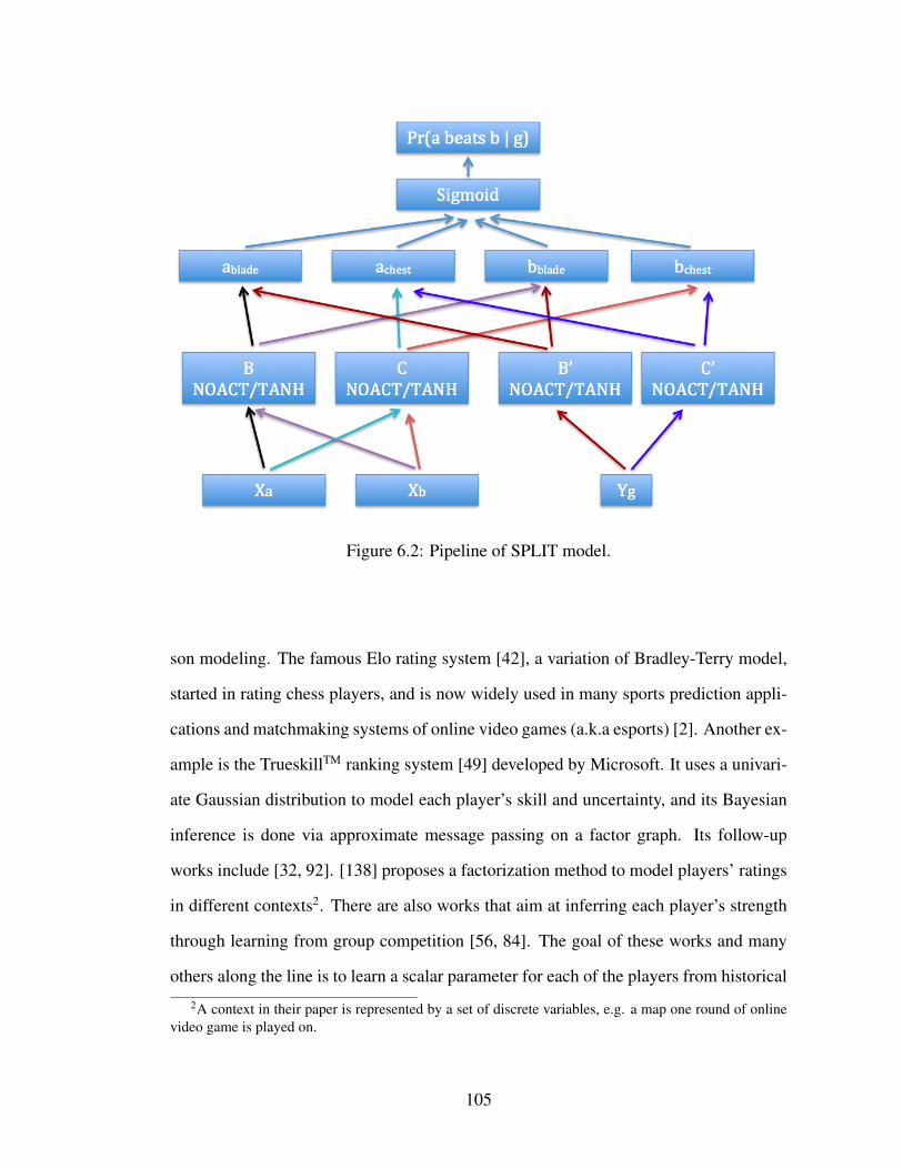
Figure 6.2: Pipeline of SPLIT model.

son modeling. The famous Elo rating system [42], a variation of Bradley-Terry model,

started in rating chess players, and is now widely used in many sports prediction appli-

cations and matchmaking systems of online video games (a.k.a esports) [2]. Another ex-

ample is the TrueskillTM ranking system [49] developed by Microsoft. It uses a univari-

ate Gaussian distribution to model each player’s skill and uncertainty, and its Bayesian

inference is done via approximate message passing on a factor graph. Its follow-up

works include [32, 92]. [138] proposes a factorization method to model players’ ratings

in different contexts2. There are also works that aim at inferring each player’s strength

through learning from group competition [56, 84]. The goal of these works and many

others along the line is to learn a scalar parameter for each of the players from historical

2A context in their paper is represented by a set of discrete variables, e.g. a map one round of onlinevideo game is played on.

105

pairwise comparison data. These parameters usually represent the absolute strengths of

individuals, with larger values favored for the win over smaller values in future games.

However, these types of models could be an oversimplification. They fail to cap-

ture things like intransitivity (rock-paper-scissors relation) that could exist in the data

[26]. To remedy it, many works attempt to use more expressive ways to model the play-

ers, and report improved performance. [25, 26] use one or more vectors to represent a

player, and are able to explicitly model the intransitive behaviors. [59, 123] generalize

Bradley-Terry model with vectorized representations of player’s ranking. The previ-

ously discussed [56] could also fall into this category, as the player is represented by

a vector of its ratings for different discrete contexts. [3] designs a matrix factorization

algorithm to predict scores of professional basketball games.

The BalanceNet model proposed in [34] is closely related to our work. It uses a

multi-layer neural network to help matchmaking in Ghost Recon Online, a first-person

shooter (FPS) online video game developed by Ubisoft. It can also account for player

features such as number of matches played, average kill/death ratio etc. The main dif-

ferences that make it incomparable with our work are twofold: For one thing, the game

they addressed is asymmetric. The opposing players in one match are playing different

roles, which means if you switch the input of them, you do not get one minus your pre-

vious probability. This comes with the nature of Ghost Recon Online, and makes it not

applicable to general symmetric matchups, unlike our framework3. For the other, it is

not built to make use of any game features.

Most of the aforementioned works on player modeling and game prediction only

take into account players’ identities, with exceptions of [56] considering discrete context

3We would argue that a symmetric matchup is a more general form, as if the game is asymmetric, itcould still be modeled as a symmetric one. One possible approach could be adding to the player featurevector to specify what asymmetric role he is playing in this game.

106

variables and [34] using additional player features. Different from them, our work in this

chapter is a general probabilistic matchup modeling framework for any two-player game

with more expressive power than player-ranking. It can also utilize any vectorized player

features and game features, no matter whether the features are discrete or continuous.

Another application of pairwise comparison is preference learning [37, 28, 135].

Instead of one player beating the other, here one observation in the dataset is one item

being preferred (by a human) over the other. In a typical preference learning setting,

the training data consists of pairwise preferences of instances, represented by a feature

vector. The goal is to learn an underlying ranking function (with scalar output) that

satisfies the training data as much as possible. A similar idea arises in the context of

search engine. It is studied as the “learning from implicit feedback problem” [29, 60,

98, 61], where user expresses his/her preference by clicking on retrieved items. The

major difference between these works and our work is threefold: Firstly, the items’

identities are usually not part of the feature vectors in their empirical tests (although

theoretically can be). Other auxiliary features are used instead. Secondly, similar to

the aforementioned player-ranking models, they try to learn a scalar ranking function

for the instance, which has limited expressiveness in representing the relations between

items. Lastly, there is no notion or no natural way of accounting for context information

in which the choice is made.

Learning with context has been studied in the machine learning community, and one

line of research that is related to our work is context-aware recommender system. While

traditional recommender system [105] considers only the ratings of a users giving to the

items4, people realize that scenarios or contexts in which users rate the items could be a

crucial factor that impacts the evaluation [4]. There is also evidence from the research in

decision-making domain that different contexts can change human decision significantly

4Works that make use of the inherent features of users and items also exist [5, 117]

107

[112, 58]. As a result, making use of the context information could significantly boost

the performance of the recommender system, as reported in representative works like [8,

66, 110, 102]. Here, the task is by learning from user’s scores of items within different

contexts to predict any missing values, the unknown score for any triple of user, item

and context. It is usually measured by mean average error (MAE) on the scores, or

normalized discounted cumulative gain (NDCG) for retrieval tasks. This differs from

the goal of our work, which is to predict the choice and its probability of pairwise

preference, not the ratings for items, as accurately as possible.

6.5 Experiments

In this section, we discuss our empirical results in the two domains: competitive

matchup data and pairwise preference data. In each domain, we report results on both

real-world data to show the applicability, and on synthesized data to demonstrate the

expressive power of our model.

6.5.1 Experiment setup

We first introduce the general setup of all the experiments. If not specified otherwise,

the experiments are run as following: We train various models (both ours and base-

lines) with different d’s (where applicable) and regularization intensities5 on the training

dataset. The model that reports the best performance on validation dataset in terms of

log-likelihood is then tested on the testing dataset.

5The selection of these hyperparameters is through grid search, with d from 2 to 100, and the sharedregularization hyperparameter λ across all parameter matrices from 1E-7 to 1E3.

108

For evaluation, we use the same two metrics as in the last chapter: average test log-

likelihood and test accuracy. The average test log-likelihood is defined similarly to the

training log-likelihood. For the test partition D′, assuming a is the winner,

L(D′|Θ) =1|D′|

∑(a,b,g)∈D′

log(Pr(a beats b|Θ, g)), (6.13)

where |D′| is the total number of games in the testing set. Log-likelihood is always a

negative value. The test accuracy is defined as

A(D′|Θ) =1|D′|

∑(a,b,g)∈D′

1Pr(a beats b|Θ,g)≥0.5. (6.14)

1· is the indicator function. This metric is a real number in [0, 1], representing the

percentage of matches whose binary outcomes can be correctly predicted according to

the model. For both metrics, the higher the value is, the better the model performs.

For the baselines, we compare our methods with rote, Bradley-Terry, pairwise lo-

gistic model and TrueskillTM. For our methods, we also vary the information we in-

put into the models, from featureless (Section 6.3.1), player/item features only to both

player/item features and game/context features.

6.5.2 Experiments with synthetic datasets

We would like to first demonstrate our models’ expressiveness on a collection of syn-

thetic datasets. In construction of these datasets, we add interpretable player/item fea-

tures and game/context features that correspond to plausible real-world scenarios.

109

Data generation

For the competitive matchup modeling, we simulate how the home-field advantage and

weather could affect the outcome of the game. Specifically, the home-field advantage

gives the home player an edge. The weather makes the matchup deterministic when it

is good, and unpredictable when it is bad. The details of the generation process are as

following:

1. There are 50 players in total.

2. There are 3 player features (in addition to player’s identity): playing at home,

playing away or playing in a neutral environment. In any game, one of the fol-

lowing is true: One player is at home and the other is away, or both players are

playing in neutral environments. The two scenarios are equally likely.

3. There are 2 game features: weather being normal or special. Each happens 50%

of the times.

4. For each possible matchup, we assign a 75/25 chance for each player to win

prior to considering the weather and home-field advantage. The favored player is

selected via a coin toss.

5. There are two types of how weather affect the games we would like to explore:

For both types, if the weather is normal, the matchup stays 75/25. For the first

type, if the weather is special (meaning bad in this case), we set the matchup to

be 50/50 and then consider the home-field’s effect. For the second type (special

weather means good), we set the matchup to be 100/0 and disregard the home-

field feature, meaning the favored player will win for sure. One can consider

that the two types simulate the two ends of the spectrum: The weather makes

the matchup extremely random or extremely deterministic. We denote the two

110

resulting datasets as syn-rand and syn-determ.

6. If one player has the home-field advantage, their chances of winning increase

by 10 percent (e.g. a 75/25 matchup when the favored player is away becomes

a 65/35 matchup). If neither player has the home-field advantage (both are in

neutral), there is no such effect.

7. For each game, we randomly sample two different players, the home-field and the

weather features. We then sample the outcome according to the resulting matchup.

8. We vary the total number of games to generate datasets with different sizes. Ev-

ery dataset is randomly divided into training, validation and testing in a roughly

5: 2 : 3 ratio.

In the domain of pairwise preference, we explore a case when different attributes

of an item affect the comparison. Imagine a case when we need to choose a restaurant

from a pair using an online recommendation system. If we are already in town and log

on a mobile device, the distance to the restaurants may be the most important factor in

the decision. On the other hand, if we are still at home with a desktop, the quality of the

restaurant may overweigh the distance, as we need to drive anyway. We generate simple

datasets to simulate this scenario:

1. We have 50 restaurants in total.

2. Each restaurant is associated with two binary 0/1 numbers that represent distance

and quality. The chance for each number to be 0 or 1 is 50%.

3. For each pairwise comparison, we uniformly select two restaurants and the mo-

bile/desktop context. We compare the two 0/1 numbers of the given context. If

they are the same, we select the winner via a coin toss. Otherwise, the one with

larger number (1 in this case) wins the comparison.

111

4. We generate datasets with various sizes, and also have a roughly 5: 2 : 3 training,

validation and testing ratio. We name the datasets syn-attr.

Empirical results

We test our models with different input information, and tune them across all training

option combinations (NOACT, TANH, CONCAT, SPLIT) on validation set. This ends

up with “featureless” (no additional feature used other than identities), “player only”

(best result by using only player features) and “our best” (best result by using both player

and game features). We compare the results against the aforementioned baselines. Note

that “player only” and “logistic” do not apply to the preference data, as there are no

player/item features other than identity. They are essentially the same as “featureless”

and “Bradley-Terry”.

We plot the performance metrics against the size of the dataset in Figure 6.3, 6.4 and

6.5. In addition, we introduce two limits, denoted as “theoretical best” and “theoretical

best rote”. For the first, it is the limit we could get by being fully aware of how the

data is generated and having an infinite amount of training and testing data. For the

second, it is similar to “theoretical best”, but the infinite amount of data only contains

players’ identities. This is is similar to featureless, Bradley-Terry, TrueskillTM and rote

baselines input-wise. Note that due to the fact that all the generated datasets are finite, it

is possible for any method that learns from them to go above the limits that is assuming

infinite data due to sampling error (It is the case in the right panel of Figure 6.5). Also,

for the right panel of Figure 6.4, the two limits overlap.

How do our models compare against the baselines? We observe that our models

generally outperform all the baselines. With full information, our models are signifi-

112

Figure 6.3: Average log-likelihood (left panel) and test accuracy (right panel) onsyn-rand datasets.

Figure 6.4: Average log-likelihood (left panel) and test accuracy (right panel) onsyn-determ datasets.

Figure 6.5: Average log-likelihood (left panel) and test accuracy (right panel) onsyn-attr datasets.

113

cantly better than the rest in terms of log-likelihood, and almost always better in terms

of accuracy. The only exception is test accuracy for syn-determ data in the right panel

of Figure 6.4, where it is fairly easy to predict the win/loss correctly since there are so

many 100/0 matchups generated. Some of the baselines go above “our best” by very

small margin, but all of them are bounded near “theoretical best”.

How do different levels of input information affect our models? In general, we

see that extra information helps improve the performance when comparing the curves

of “ours best”, “player only” and “featureless” in all plots, especially as the numbers of

games grow. It is interesting to point out that including player feature only does not help

much when comparing against featureless baselines on syn-determ data, as the “player

only” curve is barely above “featureless” in the left panel of Figure 6.4. This is due to

the way in which the dataset is generated (when weather is good, home-field advantage

is ignored, and the better player wins).

How do our models compare against the theoretical limits? On the syn-rand data

where bad weather makes game much more unpredictable, it seems that more games are

needed for “featureless” to approach “theoretical best rote” (the two curves are still very

noticeably apart at the right end in Figure 6.3). Other than that we can see our methods

tend to converge to the corresponding theoretical limits as the numbers of games grow in

all plots: in all the six plots, “our best” curves tend to get arbitrarily close to “theoretical

best”. This is evident that our methods are able to capture the underlying generation

process that is hidden from training.

114

6.5.3 Experiments with real-world datasets

Now we turn to the real-world applications. The datasets we use here also come from

the two domains: Tennis data and Starcraft II data for competitive matchup, and three

datasets from context-aware recommender system research for pairwise preference.

Tennis datasets

We first look at the data of matches between top male tennis players in the world from

year 2005-2015 and female players from year 2007-2015. These games are from all

levels of tournaments organized by Association of Tennis Professionals (ATP)6 and

Women’s Tennis Association (WTA)7. The full collection of data can be found at

http://tennis-data.co.uk/alldata.php. It contains match history of in

total 914 players and 28, 054 games for ATP, and 775 players and 21, 488 games for

WTA. For the experiments, we use the games before (including) the year 2012 for

training and validation, and the later games for testing. The training/validation ratio

is roughly 4: 1. We end up with 17, 622 training games, 4, 401 validation games and

6, 031 testing games for ATP, and 11, 725 training games, 2, 928 validation games and

6, 835 testing games for WTA.

The data source above also contains more detailed information about the players and

games, which serves as feature vectors in our model. For player features we have

1. Player’s identity;

2. World ranking when the game was played;

3. Points for world ranking when the game was played;6http://www.atpworldtour.com/7http://wtatennis.com/

115

4. Whether on a winning/losing streak;

5. Odds from several betting companies/websites: Bet3658, Expekt9, Ladbrokes10,

Pinnacles Sports11 and Stan James12.

The game features contain

1. The location at which the game took place;

2. The series the game belongs to (e.g. International Gold, Masters);

3. Indoor or outdoor court;

4. Surface of the court (e.g. Grass, Clay, Hard, Carpet);

5. The round the game was in (e.g. Group stage, Round of 16, Semifinal, Final);

6. Format of the game (usually best of 3 or best of 5).

In total, we extracted 927 player features for ATP and 788 for WTA. We also have

119 games features. As one can see from above that most of the features are discrete,

these feature vectors are very sparse.

Starcraft II dataset

We also use the Starcraft II data from Section 5.4.3. We crawled Starcraft II competition

data from a third-party website aligulac.com from the beginning of their database

to April 8th, 2015. It contains 129, 005 matches among 4, 761 professional Starcraft II

players from various online and offline tournaments. They are randomly divided into

8http://www.bet365.com/9https://www.expekt.com/

10http://www.ladbrokes.com/11http://www.pinnaclesports.com/en/12http://www.stanjames.com/

116

training, validation, testing sets according to a roughly 5: 2 : 3 ratio, giving us 64, 505

for training, 25, 800 for validation, and 38, 700 for testing. The reason we did not divide

them according to some chronological order like the tennis data is because the game is

evolving. There are at least two major stages of the game: the original release of the

game with the subtitle Wings of Liberty (WoL), and an expansion three years later called

Heart of the Swarm (HotS). Within each stage, there are many patches that modify the

rules, the units or the maps to make the game more balanced and enjoyable. Some of

these patches are more important than the others. By mixing up all games, we eliminate

the possibility that the training and testing parts being based on very different phases of

the game.

The website aligulac.com also contains rich information about these games,

from which we select a few that we think to be the most informative. There are 4, 851

player features, including

1. Player’s identity;

2. Player’s in-game race;

3. Player’s nationality13;

4. Player’s rating and standard deviation from aligulac.com;

5. Player’s rating and standard deviation versus opponent’s race from aligulac.

com.

We also end up with 40 game features, including

1. The stage of the game (WoL or HotS);

13We think it is an important feature as the Starcraft II competitive scene is mostly dominated byKorean players.

117

2. Game being played online or offline;

3. The quarter of the year in which the game was played;

4. Various keyword features contained in the event names that appear most often. For

example Group, Qualifier, Invitational, Europe, ProLeague, Playoff, Dreamhack,

etc.

Datasets from context-aware recommender system research

For our experiments, the ideal setting for collecting the data would be presenting two

choices to a human judge in various context and ask them to pick one over the other.

However, there is no such a dataset that is publicly available as far as we know. Instead,

we take the datasets for the context-aware recommender system and process them into

the format we need. In these datasets, each entry is a user’s rating for a given item under

certain context. We group all the entries by user and context. Within each group, for

any two items with different ratings, we can generate a pairwise comparison along with

the context. The datasets we use are:

1. The Food dataset from [94]. It contains 4, 036 comparisons among 20 food menus

from 212 users14. The user are in three different levels of hunger, each of which

could either be real or supposed situation.

2. The Tijuana restaurant dataset from [100]. It is a dataset of 50 people taking

questionnaires about their preference on 40 nearby restaurants. There are two

different contexts: time (weekday or weekend) and location (at school, work or

home) when the options are provided. We generate 4, 041 comparisons in total.

14We directly use the data processed by [91], which can be found at https://github.com/trungngv/gpfm

118

3. The DePaul movie dataset from [140]. 97 students of DePaul University partici-

pated in an online survey regarding 79 movies for different occasions. The context

contains time (weekday, weekend or N/A), location (home, cinema or N/A) and

companion (alone, partner, family or N/A). We create 26, 264 comparisons out of

the original data.

Similarly, each dataset is randomly divided into training, validation and testing in a

roughly 5: 2 : 3 ratio.

Empirical results

The results are in Table 6.1, 6.2, 6.3 and 6.4. In each table, we separate the baselines

and our methods with a horizontal double line. In the lower section for our models, dif-

ferent training options are blocked and ordered according to increasing information for

training: featureless for using only player/item’s identity, NOACT and TANH for using

all the player/item features, and the rest for using both player/item and game/context

features. There are fewer rows in Table 6.3 and 6.4 than in Table 6.1 and 6.2. This is

because we do not have additional item feature there and therefore some methods are

essentially the same.

How do our models compare against the baselines across different applications?

Overall, our methods are favored against all the baselines. In all of the four tables,

the best results appear in the sections of our models that use all information available.

When comparing our best results among “TANH” and “NOACT” with pairwise logistic

regression, all of which only use player features, ours are also always better. On the

other hand, our featureless model do not always beat its featureless counterparts in the

baselines. This is similar to what we found in the last chapter, where we need to include

119

Model ATP WTA Starcraft IIrote −0.6764 −0.6873 −0.5831

Bradley-Terry −0.6092 −0.6721 −0.5778TrueskillTM −0.6209 −0.6643 −0.6001

logistic −0.5777 −0.6229 −0.5808featureless −0.6590 −0.6722 −0.5886NOACT −0.5974 −0.6174 −0.5299TANH −0.5633 −0.5874 −0.5232

NOACT CONCAT −0.5970 −0.6166 −0.5229TANH CONCAT −0.5616 −0.5865 −0.5177NOACT SPLIT −0.6051 −0.6283 −0.5249TANH SPLIT −0.5981 −0.6228 −0.5178

Table 6.1: Test log-likelihood on competitive matchup datasets.

Model ATP WTA Starcraft IIrote 55.63% 53.52% 68.77%

Bradley-Terry 66.66% 61.26% 69.21%TrueskillTM 66.97% 61.96% 69.82%

logistic 69.89% 68.02% 71.68%featureless 63.70% 58.45% 73.08%NOACT 69.72% 68.09% 73.75%TANH 70.35% 68.46% 74.07%

NOACT CONCAT 69.86% 68.20% 74.22%TANH CONCAT 70.40% 68.62% 74.66%NOACT SPLIT 69.41% 67.18% 73.87%TANH SPLIT 69.87% 68.11% 75.10%

Table 6.2: Test accuracy on competitive matchup datasets.

Model Food Tijuana DePaulrote −0.6943 −0.7371 −0.6255

Bradley-Terry −0.6927 −0.6929 −0.6082TrueskillTM −0.6720 −0.7014 −0.5916featureless −0.6750 −0.6864 −0.6009

NOACT CONCAT −0.6709 −0.4321 −0.6033TANH CONCAT −0.6709 −0.4108 −0.5038NOACT SPLIT −0.6741 −0.5597 −0.5927TANH SPLIT −0.6701 −0.4207 −0.5531

Table 6.3: Test log-likelihood on pairwise preference datasets with context.

120

Model Food Tijuana DePaulrote 59.08% 50.33% 65.60%

Bradley-Terry 58.33% 54.79% 66.69%TrueskillTM 57.59% 75.33% 67.67%featureless 59.08% 58.00% 68.21%

NOACT CONCAT 57.34% 81.85% 68.29%TANH CONCAT 57.26% 82.10% 75.56%NOACT SPLIT 58.75% 80.53% 71.13%TANH SPLIT 60.81% 80.36% 73.13%

Table 6.4: Test accuracy on pairwise preference datasets with context.

a Bradley-Terry-like bias term in our model in order to surpass the baselines on certain

datasets. In terms of the extent of improvement over the best baselines, the results on

Starcraft II, Tijuana and DePaul stand out.

How do additional player features affect the models? Comparing “featureless”

with NOACT/TANH in Table 6.1 and 6.2, we can see the positive effect of adding ad-

ditional player features. Moreover, the player features we use for tennis seem to be

more influential than those used for Starcraft II (more than 5% boost versus about 1%

in accuracy). Our conjecture is that the world ranking and points features, as well as

the betting companies’ odds features are the ones responsible. By using them, we are

bootstrapping from other unknown prediction models in some sense. To test it, we run

experiments while withholding some of these features. The results on ATP and WTA

are quite similar: when the betting odds features are withheld, the performance drops

to around halfway in between TANH and “featutreless”. On the other hand, it is only

slightly pushed down when the world ranking and points features are withheld. This

suggests that the betting odds features are crucial in the improvement of performance

on tennis data.

Does the contextual information have different effects in the two domains?

Yes. Looking at the improvements between the best results with and without the

121

game/context features, it seems the preference modeling, especially on Tijuana and De-

Paul, benefits more. In terms of accuracy, they both gain about 8%, while on matchup

data it is around 1%. This suggests that in competition, the winning or losing depends

more on the players’ intrinsic properties than the environmental factors, while for hu-

man preference, the context in which the decision is made plays a much more important

role.

Which training options are preferred? TANH is always better than NOACT for

both measuring metrics and on all the datasets. When it comes to the choice between

CONCAT and SPLIT, it is not so absolute. There are few occasions where SPLIT beats

CONCAT as the bold numbers suggest, but usually not by a lot. On the other hand,

SPLIT can be outperformed by the methods without using contextual features, on the

tennis datasets for example. As a result, we would suggest TANH CONCAT to be the

go-to option of our model.

6.6 Conclusions and extensions

We present in this chapter a general probabilistic framework for modeling competi-

tive matchup and pairwise preference that can utilize any vectorized player/item and

game/context features. We conduct experiments on synthetic datasets that simulate plau-

sible real-world scenarios in both domains. The results demonstrate that our models,

while outperforming the baselines, can also approach the theoretical best limit as the

number of games/comparisons grows. Experimental results on the real-world datasets

also clearly demonstrate the advantage of our models and the benefit of utilizing the ad-

ditional features. It is interesting to see that the contextual features are more influential

in the preference domain than in competitive matchup.

122

In the end, we would like to discuss two possible extensions of this work, one for

each domain. In the domain of matchup modeling, two-team competition is a format

that is as popular as two-player game if not even more, with many major ball games

(e.g. soccer, basketball, baseball) and esports (e.g. League of Legends, Defense of the

Ancients, Counter Strike) as examples. People have attempted to model a team from

the players [56, 49, 34]. However, most of the existing models simply add the play-

ers’ rankings or other attributes to get the team’s, disregarding any synergy or chemistry

among teammates. We believe that our framework provides an option in modeling the

team with more sophisticated feature design. Using basketball as an example, we could

have a feature that is a function (e.g. product) of the point guard’s passing ability and

the center’s finish-at-the-rim ability, or the maximum of shooting guard’s and small for-

ward’s athleticism as an indicator of the team’s fastbreak strength. All of these features

are natural input of our model. Unfortunately, we do not have any empirical test results

due to lack of relevant data.

For preference learning, it would be interesting to investigate how choice from more

than two options should be modeled. One notable motivating example is the decoy effect

[58, 1], which states that a customer’s preference over two items is likely to change

when a third option is introduced that is asymmetrically dominated. For example15, an

MP3 player A that costs $400 and has 30GB storage may have similar market share

as B that costs $300 and has 20GB storage. However, after introducing the decoy C

of $450 and 25GB that is dominated by A but not B, customers’ preference tends to

shift over to A. Our current framework can directly learn from these data by treating A

and B as items, and the decoy C (existence or non-existence) as the context. However,

there is one drawback. The decoy works only when most people do not realize it is a

decoy, and this suggests that treating options differently in the model should be avoided.

15Direct paraphrasing from [1].

123

Thus, extension of our framework to handle choice among multiple items could be an

interesting direction for the future work.

124

CHAPTER 7

CONCLUSION AND FUTURE WORK

We present two lines of applications of representation learning in this thesis:

sequence and comparison, with novel applications to music playlist modeling and

matchup/preference prediction.

For the first line, we introduce the LME model in Chapter 3 for learning repre-

sentations for sequences, with music playlist modeling as the main example. It does

not require any content features of songs, and learns from coherent playlists to place

the songs into an Euclidean space. The closeness in the Euclidean space reflects the

similarity between songs as shown in the plot of the 2-dimensional embedding. Further-

more, we demonstrate LME’s advantage over several conventional language modeling

methods in terms of prediction performance, and investigate where we win over them.

To overcome the inefficiency in training the LME model with large collections of

songs, we propose Multi-LME in Chapter 4, a model that breaks up the original mono-

lithic LME model into multiple local ones in different spaces and have narrow interfaces

called “portals” to link them. All the local LME models can be trained in parallel on

different computer nodes without any communication in between. Empirically, we show

that the Multi-LME model significantly speed up the training without losing too much

model fidelity.

For the second line of application, we study representation learning in pairwise com-

parison. In Chapter 5, we propose the blade-chest model. It uses dual vectors to repre-

sent each player, one for offense (blade) and the other for defence (chest). It is capable

of modeling any matchup probabilities among any players including the intransitivity,

which many conventional rank-based methods fail to model. We have tested the model

125

on a wide range of applications and datasets, and observe general improvements across

the board, especially in the domain of online competitive video games.

We then follow up the blade-chest model in Chapter 6, introducing a general prob-

abilistic framework for predicting pairwise comparison with both object and context

features. We examine it in the context of matchup and pairwise preference prediction.

With empirical results on several synthetic and real-world datasets that are generally

favorable against the baseline models, we show the expressiveness and applicability of

our framework.

Overall, this thesis work proposes novel models of representation learning methods

in sequence and comparison modeling, with their effectiveness theoretically analyzed

and empirically tested. We believe it is a meaningful step towards broadening the scope

of representation learning.

For the future work of this thesis, we can think of two levels of directions. For

one, which is the concrete level, one could extend the models presented in previous

chapters, which have already been discussed individually. They include modeling long-

range dependencies in sequences, incorporating general content and meta features of

songs into LME and developing efficient training method for it, personalized playlist

modeling, matchup prediction for team-based sports/games, non-rank-based preference

modeling for multiple items. For the other, the high-level direction, we can view any

data that we want to apply representation learning methods on as being composed of

objects and the interactions among them. The objects and interactions can be effectively

represented by graphs, or generalization of graphs such as multigraphs (multiple edges

are allowed between the same pair of vertices; edge that connects a vertex and itself

is allowed) or hypergraphs (an edge could connect multiple vertices) [7]. To make it

more general, each vertex that stands for an object could be associated with its features.

126

Moreover, the context could also be considered. One possible way is to represent context

via virtual objects along with the interaction edges that link to the real objects. By

thinking this way, we can abstract many representation learning problems to a general

graph embedding problem with vertex features. We believe studying this general form

as well as its efficient training method could shed light on each of its instantiations, and

also further expand the scope of representation learning.

127

BIBLIOGRAPHY

[1] Wikipedia page on decoy effect. https://en.wikipedia.org/wiki/Decoy_effect.

[2] Wikipedia page on elo rating system. https://en.wikipedia.org/wiki/Elo_rating_system.

[3] Ryan Prescott Adams, George E Dahl, and Iain Murray. Incorporating side in-formation in probabilistic matrix factorization with gaussian processes. arXivpreprint arXiv:1003.4944, 2010.

[4] Gediminas Adomavicius, Ramesh Sankaranarayanan, Shahana Sen, and Alexan-der Tuzhilin. Incorporating contextual information in recommender systems us-ing a multidimensional approach. ACM Transactions on Information Systems(TOIS), 23(1):103–145, 2005.

[5] Deepak Agarwal and Bee-Chung Chen. Regression-based latent factor models. InProceedings of the 15th ACM SIGKDD international conference on Knowledgediscovery and data mining, pages 19–28. ACM, 2009.

[6] N. Aizenberg, Y. Koren, and O. Somekh. Build your own music recommenderby modeling internet radio streams. In Proceedings of the 21st internationalconference on World Wide Web, pages 1–10. ACM, 2012.

[7] VK Balakrishnan. Schaum’s Outline of Graph Theory: Including Hundreds ofSolved Problems. McGraw Hill Professional, 1997.

[8] Linas Baltrunas and Francesco Ricci. Context-based splitting of item ratings incollaborative filtering. In Proceedings of the third ACM conference on Recom-mender systems, pages 245–248. ACM, 2009.

[9] Cyrille Barrette and Denis Vandal. Social rank, dominance, antler size, and accessto food in snow-bound wild woodland caribou. Behaviour, pages 118–146, 1986.

[10] L. Barrington, R. Oda, and G. Lanckriet. Smarter than genius? human evaluationof music recommender systems. ISMIR, 2009.

[11] Mikhail Belkin and Partha Niyogi. Laplacian eigenmaps and spectral techniquesfor embedding and clustering. In NIPS, volume 14, pages 585–591, 2001.

128

[12] Yoshua Bengio, Aaron Courville, and Pierre Vincent. Representation learning: Areview and new perspectives. Pattern Analysis and Machine Intelligence, IEEETransactions on, 35(8):1798–1828, 2013.

[13] Yoshua Bengio, Jean-Francois Paiement, Pascal Vincent, Olivier Delalleau, Nico-las Le Roux, and Marie Ouimet. Out-of-sample extensions for lle, isomap, mds,eigenmaps, and spectral clustering. Mij, 1:2, 2003.

[14] Yoshua Bengio, Holger Schwenk, Jean-Sebastien Senecal, Frederic Morin, andJean-Luc Gauvain. Neural probabilistic language models. Innovations in Ma-chine Learning, pages 137–186, 2006.

[15] Yoshua Bengio, Patrice Simard, and Paolo Frasconi. Learning long-term depen-dencies with gradient descent is difficult. Neural Networks, IEEE Transactionson, 5(2):157–166, 1994.

[16] Jeff Bilmes, Gang Ji, and Marina Meila. Intransitive likelihood-ratio classifiers.In NIPS, pages 1141–1148, 2001.

[17] Christopher M Bishop. Pattern recognition and machine learning. springer, 2006.

[18] David M Blei, Andrew Y Ng, and Michael I Jordan. Latent dirichlet allocation.the Journal of machine Learning research, 3:993–1022, 2003.

[19] Leon Bottou. Stochastic learning. In Advanced lectures on machine learning,pages 146–168. Springer, 2004.

[20] Leon Bottou. Large-scale machine learning with stochastic gradient descent. InProceedings of COMPSTAT’2010, pages 177–186. Springer, 2010.

[21] Ralph Allan Bradley and Milton E Terry. Rank analysis of incomplete blockdesigns: I. the method of paired comparisons. Biometrika, pages 324–345, 1952.

[22] Miguel A Carreira-Perpinan and Geoffrey E Hinton. On contrastive divergencelearning. In Proceedings of the tenth international workshop on artificial intelli-gence and statistics, pages 33–40. Society for Artificial Intelligence and StatisticsNP, 2005.

[23] Manuela Cattelan et al. Models for paired comparison data: A review with em-phasis on dependent data. Statistical Science, 27(3):412–433, 2012.

129

[24] Manuela Cattelan, Cristiano Varin, and David Firth. Dynamic bradley–terry mod-elling of sports tournaments. Journal of the Royal Statistical Society: Series C(Applied Statistics), 62(1):135–150, 2013.

[25] David Causeur and Francois Husson. A 2-dimensional extension of the bradley–terry model for paired comparisons. Journal of statistical planning and inference,135(2):245–259, 2005.

[26] Shuo Chen and Thorsten Joachims. Modeling intransitivity in matchup and com-parison data. In Proceedings of The 9th ACM International Conference on WebSearch and Data Mining (WSDM). ACM, 2016.

[27] Shuo Chen, Jiexun Xu, and Thorsten Joachims. Multi-space probabilistic se-quence modeling. In Proceedings of the 19th ACM SIGKDD international con-ference on Knowledge discovery and data mining, pages 865–873. ACM, 2013.

[28] Wei Chu and Zoubin Ghahramani. Preference learning with gaussian processes.In Proceedings of the 22nd international conference on Machine learning, pages137–144. ACM, 2005.

[29] William W Cohen, Robert E Schapire, and Yoram Singer. Learning to orderthings. In Advances in Neural Information Processing Systems 10: Proceedingsof the 1997 Conference, volume 10, page 451. MIT Press, 1998.

[30] T. F. Cox and M. A. Cox. Multidimensional scaling. Chapman and Hall, 2001.

[31] Trevor F Cox and Michael AA Cox. Multidimensional scaling. CRC Press, 2000.

[32] Pierre Dangauthier, Ralf Herbrich, Tom Minka, Thore Graepel, et al. Trueskillthrough time: Revisiting the history of chess. In NIPS, 2007.

[33] Ofer Dekel, Ran Gilad-Bachrach, Ohad Shamir, and Lin Xiao. Optimal dis-tributed online prediction using mini-batches. The Journal of Machine LearningResearch (JMLR), 13:165–202, 2012.

[34] Olivier Delalleau, Emile Contal, Eric Thibodeau-Laufer, Raul Chandias Ferrari,Yoshua Bengio, and Frank Zhang. Beyond skill rating: Advanced matchmak-ing in ghost recon online. Computational Intelligence and AI in Games, IEEETransactions on, 4(3):167–177, 2012.

[35] John Duchi, Elad Hazan, and Yoram Singer. Adaptive subgradient methods for

130

online learning and stochastic optimization. The Journal of Machine LearningResearch, 12:2121–2159, 2011.

[36] George Skaff Elias, Richard Garfield, and K Robert Gutschera. Characteristicsof games. MIT Press, 2012.

[37] Johannes Furnkranz and Eyke Hullermeier. Preference learning. Springer, 2010.

[38] Edgar Gabriel, Graham E. Fagg, George Bosilca, Thara Angskun, Jack J. Don-garra, Jeffrey M. Squyres, Vishal Sahay, Prabhanjan Kambadur, Brian Barrett,Andrew Lumsdaine, Ralph H. Castain, David J. Daniel, Richard L. Graham, andTimothy S. Woodall. Open MPI: Goals, concept, and design of a next generationMPI implementation. In Proceedings, 11th European PVM/MPI Users’ GroupMeeting, pages 97–104, Budapest, Hungary, September 2004.

[39] William V Gehrlein. The probability of intransitivity of pairwise comparisons inindividual preference. Mathematical social sciences, 17(1):67–75, 1989.

[40] David F Gleich and Lek-heng Lim. Rank aggregation via nuclear norm mini-mization. In Proceedings of the 17th ACM SIGKDD international conference onKnowledge discovery and data mining, pages 60–68. ACM, 2011.

[41] David F. Gleich, Leonid Zhukov, Matthew Rasmussen, and Kevin Lang. TheWorld of Music: SDP embedding of high dimensional data. In Information Visu-alization 2005, 2005.

[42] Mark E Glickman. A comprehensive guide to chess ratings. American ChessJournal, 3:59–102, 1995.

[43] A. Globerson, G. Chechik, F. Pereira, et al. Euclidean embedding of co-occurrence data. Journal of Machine Learning Research (JMLR), 2007.

[44] Ken Goldberg, Theresa Roeder, Dhruv Gupta, and Chris Perkins. Eigentaste: Aconstant time collaborative filtering algorithm. Information Retrieval, 4(2):133–151, 2001.

[45] Gene H Golub and Charles F Van Loan. Matrix computations, volume 3. JHUPress, 2012.

[46] Prem Gopalan, Jake M Hofman, and David M Blei. Scalable recommendationwith poisson factorization. arXiv preprint arXiv:1311.1704, 2013.

131

[47] Michael Gutmann and Aapo Hyvarinen. Noise-contrastive estimation: A newestimation principle for unnormalized statistical models. In International Con-ference on Artificial Intelligence and Statistics, pages 297–304, 2010.

[48] Xiaofei He and Partha Niyogi. Locality preserving projections. In NIPS, vol-ume 16, pages 234–241, 2003.

[49] Ralf Herbrich, Tom Minka, and Thore Graepel. TrueskillTM: A bayesian skillrating system. In Advances in Neural Information Processing Systems, pages569–576, 2006.

[50] Jonathan L Herlocker, Joseph A Konstan, Al Borchers, and John Riedl. An algo-rithmic framework for performing collaborative filtering. In Proceedings of the22nd annual international ACM SIGIR conference on Research and developmentin information retrieval, pages 230–237. ACM, 1999.

[51] G. Hinton and S. Roweis. Stochastic neighbor embedding. Advances in NeuralInformation Processing Systems (NIPS), 15:833–840, 2002.

[52] Thomas Hofmann. Probabilistic latent semantic indexing. In Proceedings of the22nd annual international ACM SIGIR conference on Research and developmentin information retrieval, pages 50–57. ACM, 1999.

[53] D. Hsu, S.M. Kakade, and T. Zhang. A spectral algorithm for learning hiddenmarkov models. Arxiv preprint arXiv:0811.4413, 2008.

[54] Eric H Huang, Richard Socher, Christopher D Manning, and Andrew Y Ng. Im-proving word representations via global context and multiple word prototypes.In Proceedings of the 50th Annual Meeting of the Association for ComputationalLinguistics: Long Papers-Volume 1, pages 873–882. Association for Computa-tional Linguistics, 2012.

[55] Eric H Huang, Richard Socher, Christopher D Manning, and Andrew Y Ng. Im-proving word representations via global context and multiple word prototypes.In Proceedings of the 50th Annual Meeting of the Association for ComputationalLinguistics (ACL): Long Papers-Volume 1, pages 873–882. Association for Com-putational Linguistics, 2012.

[56] Tzu-Kuo Huang, Chih-Jen Lin, and Ruby C Weng. Ranking individuals by groupcomparisons. In Proceedings of the 23rd international conference on Machinelearning, pages 425–432. ACM, 2006.

132

[57] Tzu-Kuo Huang, Ruby C Weng, and Chih-Jen Lin. Generalized bradley-terrymodels and multi-class probability estimates. The Journal of Machine LearningResearch, 7:85–115, 2006.

[58] Joel Huber, John W Payne, and Christopher Puto. Adding asymmetrically domi-nated alternatives: Violations of regularity and the similarity hypothesis. Journalof consumer research, pages 90–98, 1982.

[59] David R Hunter. Mm algorithms for generalized bradley-terry models. Annals ofStatistics, pages 384–406, 2004.

[60] Thorsten Joachims et al. Evaluating retrieval performance using clickthroughdata., 2003.

[61] Thorsten Joachims, Laura Granka, Bing Pan, Helene Hembrooke, and Geri Gay.Accurately interpreting clickthrough data as implicit feedback. In Proceedings ofthe 28th annual international ACM SIGIR conference on Research and develop-ment in information retrieval, pages 154–161. ACM, 2005.

[62] Ian Jolliffe. Principal component analysis. Wiley Online Library, 2005.

[63] D. Jurafsky and J.H. Martin. Speech and language processing, 2008.

[64] Dan Jurafsky and James H Martin. Speech & language processing. PearsonEducation India, 2000.

[65] Toshihiro Kamishima. Nantonac collaborative filtering: recommendation basedon order responses. In Proceedings of the ninth ACM SIGKDD international con-ference on Knowledge discovery and data mining, pages 583–588. ACM, 2003.

[66] Alexandros Karatzoglou, Xavier Amatriain, Linas Baltrunas, and Nuria Oliver.Multiverse recommendation: n-dimensional tensor factorization for context-aware collaborative filtering. In Proceedings of the fourth ACM conference onRecommender systems, pages 79–86. ACM, 2010.

[67] G. Karypis and V. Kumar. A fast and high quality multilevel scheme for parti-tioning irregular graphs. SIAM Journal on Scientific Computing, 20(1):359–392,1998.

[68] Mohammad Khoshneshin and W Nick Street. Collaborative filtering via eu-clidean embedding. In Proceedings of the fourth ACM conference on Recom-mender systems (RecSys), pages 87–94. ACM, 2010.

133

[69] Jon Kleinberg and Eva Tardos. Algorithm design. Pearson Education India, 2006.

[70] Yehuda Koren, Robert Bell, and Chris Volinsky. Matrix factorization techniquesfor recommender systems. Computer, 42(8):30–37, 2009.

[71] Yehuda Koren, Robert M. Bell, and Chris Volinsky. Matrix factorization tech-niques for recommender systems. IEEE Computer, 42(8):30–37, 2009.

[72] Yann LeCun and Yoshua Bengio. Convolutional networks for images, speech,and time series. The handbook of brain theory and neural networks, 3361(10),1995.

[73] Yann LeCun, Yoshua Bengio, and Geoffrey Hinton. Deep learning. Nature,521(7553):436–444, 2015.

[74] Daniel D Lee and H Sebastian Seung. Learning the parts of objects by non-negative matrix factorization. Nature, 401(6755):788–791, 1999.

[75] Pedro Linares. Are inconsistent decisions better? an experiment with pairwisecomparisons. European Journal of Operational Research, 193(2):492–498, 2009.

[76] B. Logan. Content-based playlist generation: exploratory ex- periments. ISMIR,2002.

[77] R.. Ducan Luce. Individual Choice Behavior a Theoretical Analysis. john Wileyand Sons, 1959.

[78] F. Maillet, D. Eck, G. Desjardins, and P. Lamere. Steerable playlist generation bylearning song similarity from radio station playlists. In International Conferenceon Music Information Retrieval (ISMIR), 2009.

[79] Y. Maron, M. Lamar, and E. Bienenstock. Sphere embedding: An application topart-of-speech induction. In Neural Information Processing Systems Conference(NIPS), 2010.

[80] Kenneth O May. Intransitivity, utility, and the aggregation of preference patterns.Econometrica: Journal of the Econometric Society, pages 1–13, 1954.

[81] Brian McFee and Gert R. G. Lanckriet. Metric learning to rank. In ICML, pages775–782, 2010.

134

[82] Brian McFee and Gert R. G. Lanckriet. The natural language of playlists. InInternational Conference on Music Information Retrieval (ISMIR), 2011.

[83] Ian McHale and Alex Morton. A bradley-terry type model for forecasting tennismatch results. International Journal of Forecasting, 27(2):619–630, 2011.

[84] Joshua E Menke and Tony R Martinez. A bradley–terry artificial neural networkmodel for individual ratings in group competitions. Neural computing and Appli-cations, 17(2):175–186, 2008.

[85] Tomas Mikolov, Ilya Sutskever, Kai Chen, Greg S Corrado, and Jeff Dean. Dis-tributed representations of words and phrases and their compositionality. In Ad-vances in Neural Information Processing Systems, pages 3111–3119, 2013.

[86] Andriy Mnih and Geoffrey Hinton. Three new graphical models for statisticallanguage modelling. In Proceedings of the 24th International Conference onMachine learning (ICML), pages 641–648. ACM, 2007.

[87] J. L. Moore, Shuo Chen, T. Joachims, and D. Turnbull. Learning to embed songsand tags for playlist prediction, April 2012.

[88] J.L. Moore, Shuo Chen, T. Joachims, and D. Turnbull. Learning to embed songsand tags for playlist prediction. In International Conference on Music Informa-tion Retrieval (ISMIR), pages 349–354, 2012.

[89] Andrew Y Ng, Michael I Jordan, and Yair Weiss. On spectral clustering analysisand an algorithm. Proceedings of Advances in Neural Information ProcessingSystems. Cambridge, MA: MIT Press, 14:849–856, 2001.

[90] A.Y. Ng, M.I. Jordan, Y. Weiss, et al. On spectral clustering: Analysis and analgorithm. Advances in Neural Information Processing Systems (NIPS), 2:849–856, 2002.

[91] Trung V Nguyen, Alexandros Karatzoglou, and Linas Baltrunas. Gaussian pro-cess factorization machines for context-aware recommendations. In Proceedingsof the 37th international ACM SIGIR conference on Research & development ininformation retrieval, pages 63–72. ACM, 2014.

[92] Sergey Nikolenko and Alexander Sirotkin. A new bayesian rating system for teamcompetitions. In Proceedings of the 28th International Conference on MachineLearning (ICML-11), pages 601–608, 2011.

135

[93] Feng Niu, Benjamin Recht, Christopher Re, and Stephen J Wright. Hogwild!:A lock-free approach to parallelizing stochastic gradient descent. arXiv preprintarXiv:1106.5730, 2011.

[94] Chihiro Ono, Yasuhiro Takishima, Yoichi Motomura, and Hideki Asoh. Context-aware preference model based on a study of difference between real and supposedsituation data. UMAP, 9:102–113, 2009.

[95] Christos H Papadimitriou, Hisao Tamaki, Prabhakar Raghavan, and SantoshVempala. Latent semantic indexing: A probabilistic analysis. In Proceedingsof the seventeenth ACM SIGACT-SIGMOD-SIGART symposium on Principles ofdatabase systems, pages 159–168. ACM, 1998.

[96] John C. Platt. Fast embedding of sparse music similarity graphs. In NIPS. MITPress, 2003.

[97] L.R. Rabiner. A tutorial on hidden markov models and selected applications inspeech recognition. Proceedings of the IEEE, 77(2):257–286, 1989.

[98] Filip Radlinski and Thorsten Joachims. Query chains: learning to rank fromimplicit feedback. In Proceedings of the eleventh ACM SIGKDD internationalconference on Knowledge discovery in data mining, pages 239–248. ACM, 2005.

[99] Karthik Raman and Thorsten Joachims. Methods for ordinal peer grading. InProceedings of the 20th ACM SIGKDD international conference on Knowledgediscovery and data mining, pages 1037–1046. ACM, 2014.

[100] Xochilt Ramirez-Garcia and Mario Garcıa-Valdez. Post-filtering for a restaurantcontext-aware recommender system. In Oscar Castillo, Patricia Melin, WitoldPedrycz, and Janusz Kacprzyk, editors, Recent Advances on Hybrid Approachesfor Designing Intelligent Systems, volume 547 of Studies in Computational Intel-ligence, pages 695–707. Springer International Publishing, 2014.

[101] S. Rendle, C. Freudenthaler, and L. Schmidt-Thieme. Factorizing personalizedmarkov chains for next-basket recommendation. In Proceedings of the 19th in-ternational conference on World Wide Web (WWW), pages 811–820. ACM, 2010.

[102] Steffen Rendle. Factorization machines. In Data Mining (ICDM), 2010 IEEE10th International Conference on, pages 995–1000. IEEE, 2010.

[103] Steffen Rendle, Christoph Freudenthaler, Zeno Gantner, and Lars Schmidt-Thieme. BPR: Bayesian personalized ranking from implicit feedback. In Jeff

136

Bilmes and Andrew Y. Ng, editors, Proceedings of the Twenty-Fifth Confer-ence on Uncertainty in Artificial Intelligence (UAI), pages 452–461. AUAI Press,2009.

[104] Steffen Rendle and Lars Schmidt-Thieme. Pairwise interaction tensor factor-ization for personalized tag recommendation. In Proceedings of the third ACMinternational conference on Web search and data mining, pages 81–90. ACM,2010.

[105] Paul Resnick and Hal R Varian. Recommender systems. Communications of theACM, 40(3):56–58, 1997.

[106] Sam T Roweis and Lawrence K Saul. Nonlinear dimensionality reduction bylocally linear embedding. Science, 290(5500):2323–2326, 2000.

[107] David E Rumelhart, Geoffrey E Hinton, and Ronald J Williams. Learning repre-sentations by back-propagating errors. Cognitive modeling, 5:3, 1988.

[108] Ruslan Salakhutdinov and Andriy Mnih. Probabilistic matrix factorization. InNIPS, volume 1, pages 2–1, 2007.

[109] Blake Shaw and Tony Jebara. Structure preserving embedding. In Proceedings ofthe 26th Annual International Conference on Machine Learning, pages 937–944.ACM, 2009.

[110] Yue Shi, Alexandros Karatzoglou, Linas Baltrunas, Martha Larson, Alan Han-jalic, and Nuria Oliver. Tfmap: Optimizing map for top-n context-aware recom-mendation. In Proceedings of the 35th international ACM SIGIR conference onResearch and development in information retrieval, pages 155–164. ACM, 2012.

[111] Shuo Chen, J.L. Moore, D. Turnbull, and T. Joachims. Playlist prediction viametric embedding. In Proceedings of the 18th ACM SIGKDD international con-ference on knowledge discovery and data mining (KDD), pages 714–722. ACM,2012.

[112] Itamar Simonson and Amos Tversky. Choice in context: Tradeoff contrast andextremeness aversion. JMR, Journal of Marketing Research, 29(3):281, 1992.

[113] Barry Sinervo and Curt M Lively. The rock-paper-scissors game and the evolutionof alternative male strategies. Nature, 380(6571):240–243, 1996.

137

[114] Richard Socher, Brody Huval, Christopher D Manning, and Andrew Y Ng. Se-mantic compositionality through recursive matrix-vector spaces. In Proceedingsof the 2012 Joint Conference on Empirical Methods in Natural Language Pro-cessing and Computational Natural Language Learning, pages 1201–1211. As-sociation for Computational Linguistics, 2012.

[115] L. Song, B. Boots, S. Siddiqi, G. Gordon, and A. Smola. Hilbert space embed-dings of hidden markov models. 2010.

[116] Nathan Srebro, Jason DM Rennie, and Tommi Jaakkola. Maximum-margin ma-trix factorization. In NIPS, volume 17, pages 1329–1336, 2004.

[117] David H Stern, Ralf Herbrich, and Thore Graepel. Matchbox: large scale onlinebayesian recommendations. In Proceedings of the 18th international conferenceon World wide web, pages 111–120. ACM, 2009.

[118] Joshua B Tenenbaum, Vin De Silva, and John C Langford. A global geometricframework for nonlinear dimensionality reduction. Science, 290(5500):2319–2323, 2000.

[119] Louis L Thurstone. A law of comparative judgment. Psychological review,34(4):273, 1927.

[120] Nicolaus Tideman. Collective decisions and voting. Ashgate Burlington, 2006.

[121] D. Tingle, Y. Kim, and D.Turnbull. Exploring automatic music annotation with“acoustically-objective” tags. In ACM International Conference on MultimediaInformation Retrieval, 2010.

[122] Jarle Tufto, Erling Johan Solberg, and Thor-Harald Ringsby. Statistical models oftransitive and intransitive dominance structures. Animal behaviour, 55(6):1489–1498, 1998.

[123] Satoshi Usami. Individual differences multidimensional bradley-terry modelusing reversible jump markov chain monte carlo algorithm. Behaviormetrika,37(2):135–155, 2010.

[124] Laurens Van der Maaten and Geoffrey Hinton. Visualizing data using t-sne. Jour-nal of Machine Learning Research, 9(2579-2605):85, 2008.

[125] Lieven Vandenberghe and Stephen Boyd. Semidefinite programming. SIAM re-view, 38(1):49–95, 1996.

138

[126] Pascal Vincent, Hugo Larochelle, Yoshua Bengio, and Pierre-Antoine Manzagol.Extracting and composing robust features with denoising autoencoders. In Pro-ceedings of the 25th international conference on Machine learning, pages 1096–1103. ACM, 2008.

[127] Ulrike Von Luxburg. A tutorial on spectral clustering. Statistics and computing,17(4):395–416, 2007.

[128] C. Wang and D. Blei. Collaborative topic modeling for recommending scientificarticles. In SIGKDD, 2011.

[129] Chong Wang and David M Blei. Collaborative topic modeling for recommendingscientific articles. In Proceedings of the 17th ACM SIGKDD international con-ference on Knowledge discovery and data mining, pages 448–456. ACM, 2011.

[130] Kilian Weinberger, John Blitzer, and Lawrence Saul. Distance metric learningfor large margin nearest neighbor classification. Advances in neural informationprocessing systems, 18:1473, 2006.

[131] Kilian Q Weinberger, Benjamin D Packer, and Lawrence K Saul. Nonlinear di-mensionality reduction by semidefinite programming and kernel matrix factoriza-tion. In Proceedings of the tenth international workshop on artificial intelligenceand statistics, pages 381–388, 2005.

[132] J. Weston, S. Bengio, and P. Hamel. Multi-tasking with joint semantic spacesfor large-scale music annotation and retrieval. Journal of New Music Research,2011.

[133] Jason Weston, Samy Bengio, and Nicolas Usunier. Wsabie: Scaling up to largevocabulary image annotation. In Proceedings of the Twenty-Second internationaljoint conference on Artificial Intelligence-Volume Volume Three, pages 2764–2770. AAAI Press, 2011.

[134] Jason Weston, Sumit Chopra, and Keith Adams. #tagspace: Semantic embed-dings from hashtags. In EMNLP, 2014.

[135] Georgios N Yannakakis, Manolis Maragoudakis, and John Hallam. Preferencelearning for cognitive modeling: a case study on entertainment preferences. Sys-tems, Man and Cybernetics, Part A: Systems and Humans, IEEE Transactions on,39(6):1165–1175, 2009.

[136] Ainur Yessenalina and Claire Cardie. Compositional matrix-space models for

139

sentiment analysis. In Proceedings of the Conference on Empirical Methods inNatural Language Processing, pages 172–182. Association for ComputationalLinguistics, 2011.

[137] Yisong Yue and T. Joachims. Predicting diverse subsets using structural SVMs.In International Conference on Machine Learning (ICML), pages 271–278, 2008.

[138] Lei Zhang, Jun Wu, Zhong-Cun Wang, and Chong-Jun Wang. A factor-basedmodel for context-sensitive skill rating systems. In Tools with Artificial Intelli-gence (ICTAI), 2010 22nd IEEE International Conference on, volume 2, pages249–255. IEEE, 2010.

[139] E. Zheleva, J. Guiver, E. Mendes Rodrigues, and N. Milic-Frayling. Statisticalmodels of music-listening sessions in social media. In Proceedings of the 19thinternational conference on World wide web, pages 1019–1028. ACM, 2010.

[140] Yong Zheng, Bamshad Mobasher, and Robin Burke. Carskit: A java-basedcontext-aware recommendation engine. In Proceedings of the 15th IEEE Inter-national Conference on Data Mining Workshops. IEEE, 2015.

[141] Ding Zhou, Shenghuo Zhu, Kai Yu, Xiaodan Song, Belle L Tseng, HongyuanZha, and C Lee Giles. Learning multiple graphs for document recommendations.In Proceedings of the 17th international conference on World Wide Web (WWW),pages 141–150. ACM, 2008.

[142] Xiaojin Zhu. Semi-supervised learning literature survey. Computer Science, Uni-versity of Wisconsin-Madison, 2:3, 2006.

[143] Martin Zinkevich, Markus Weimer, Alex Smola, and Lihong Li. Parallelizedstochastic gradient descent. Advances in Neural Information Processing Systems(NIPS), 23(23):1–9, 2010.

140