i--

REPORT NO. 1954

EXPERIMENTAL MEASUREMENTS OF THE

TURBULENT BOUNDARY LAYER ON A YAWED,

SPINNING SLENDER BODY

Walter B. SturekJames E. Danberg

January 1977

FEB 7 ~

Approved for public release- distribution unlimited. .yj" U...-'

A-

USA BALLISTIC RESEARCH LABORATORIESABERDEEN PROVING GROUND, MARYLAND

C

Destroy this report when it is no !onge ';needed.Do not return It to the originator.

Secondary distribution of this report by originatingor sponsoring activity is prohibited.

Additional copies of this report may be obtainedfrom the National Technical Information Service,U.S. Department of Commerce, Springfield, Virginia22151,

The findings in this report are not to be construed asan official Department 'of the Army position, unlessso designated by other authorized documents.

UNCLASSIF:IEDSECURITY CLASSIFICATION OF THIS PAGE (WW. Onto Bneere4

REPORT DOCUMENTATION PAGE ZDWTU10151. a"WTNUMURa. GOVT ACCESSION NO: 11- RUCIPIENT'S CATALOG NUMBER

~BRL W*"NaIjrm19 5 4I OF RZPOR I aPERIOD COVERED

-L-XPERIMENTAL MEASUREMENTS OF THEJIJRBULENT X Final~OUNDARYAYEt ON A YAWED, SPINNING SLENDER

7. Ne.S. -CONTRACT Olt GRANT NUMS111(m)

eI Walte B/Stu2ekJames E./banbergj _____________

9. PER"ONMING ORG1ANIZATION NAME ANO ADDRESS 10. PR RAM ELaMENT, PROJEKCTY. TASKC

U.S. Army Ballistic Research Laboratory 4 /IWR

Aberdeen Proving Ground, Maryland 21005 R lLl6ll')0(2AH43

11. CONTROLLING OFFICE NAME AND ADDRESS J

U.S. Army Materiel Development & Readiness Comma /y' JN'.5001 Eisenhower Avenue61-Alexandria, Virginia 22333 314. MONITORING AGENCY NAME A AODRESS(if dDiI.,amt =r Cont'ollind 011100) IS. SE1CURITO's 61 e1"

U~nc lass ifiedF17 DEkASPIC ATION/ DOWN ORADING0

16. DISTRIBUTION STATEMENT (of thise Repot)

Approved for public release; distribution unlimited.

17. DISTRIBUTION STATEMENT (of the abstract eitered in Block 20, It different from Report)

Is. SUPPLEMENTARY NOTES

19. KEY WORDS (Continue on reverse side iI nececewy &mid dntif by block number)

Supersonic Turbulent Boundary LayerLaw of the WallVelocity ProfilesYawed Body of RevolutionI4 hree-Dimbnginnal wnr'lr wetI rwo&mww I

2' W. ABSTRACT (Coitomman reverse eld iiAF1 '~ u dniybySekaibr lExperimental measurements of the tripped turbulent boundary layer profilecharacteristics on a yawed, spinning tangent-ogive-cylinder model are described.The profile measurements were made "using a flattened total head probe at 30incremen tel t~t the azimuthal plane for three longitudinal stationsat M 3>-A-4 'Y#N' 10,000 RPM. Wall static pressure measurements wereobtained in order to compute velocity profiles from aJ~ measured tots head

presu e Thedat hae ben aayzed according to Alawof the wall~av of the,wake*{oncepts using a least s uare fittin technigue The effet* gind

DD0 FJT" 1473 EDITIONMOF I 06VOIIItoSOLEIR

JA I IN..S.ITI

11E LOT, CLAIPICA~tOW or ?HO ~fb DowI sme

2.ABSTRtACT (otiuued~ i4's-j

fl f aiuhlPosition is revealed in the growth of the wake parameter by afactor Of two from the wind to the lee-side. A small but consistent effectOf spin is alSO apparent.

V-4

TABLE OF CONTENTS

Page

LIST OF ILLLUSTRATIONS .................... 5

I. INTRODUCTION . . . . ... . . . . . . . 7. . . . . . . 7

II. THE EXPERIMENT ............................. 8

A. Test Facility ...... . . . . . . . . . ....... 8

B. Model . . . . . . . . . . . . . . . . . . . . . . . 8

C. Survey Mechanism . . . . . . . . ......... 9D. Test Procedure ........... ............. 9

E. Wall Static Pressure Measurements . . . . . . .10F. Data Reduction ........ ... ................ 10

III. DISCUSSION OF TH RESTS .................. . 11

IV. LAW OF THE ALL ANALYSIS ..................... 12

A. Profile Characterization ... ........... 12

B. Azimuthal Distribution of Profile Parameters ... ...... 14

V. SlIeARY'.. .. ... . . . . .. .. .. .. .. . .15i

REFERENCES . . . . . .. . . . . . . . . . . . . . . . . 17

LIST OF SYMBOLS ....... ....................... .. 27

DISTRIBUTION LIST .. . . . . . . . ........... 29

V ... .... .......... .. .

v~i i

........ ai__i i

' " '1*--*.:

7 ' , 'IL" ,i

..... " ... "".... ":"': :' :~t i ;' ...... ii ' ' :K4 '.

LIST OF ILLUSTRATIONS

Figure Pogo

1. model Geoetry. . . . 19

2. •oe Installation With Survey Mechanism. . . . . . . . . 19

3. Coordinate System . . . . . . . . . . . . . . . . . . . . 20

4. Spark Sbadograph of Flov, N 3, a 4. . . . . . . . . 20

S. Velocity Profiles, N - 3, a . 40, Z/D - 3.04 Zero Spin . . 21

6. Velocity Profiles, N * 3, a a 40, Z/D = 4.5, Zero Spin . . 21

7. Velocity Profiles, N * 3, a 40, Z/D * 6.0, Zero Spin . 21

S. Oil Flow Visualization, N. 3, a 4 4 00 . . . ... 22

9. Oil FlovVisualization, M 3, a 4, =90° . . . . . . 22

10. Oil Flow Visualization, N 3 3, a - 4', 1800 .. . . . 22

11. Wall Static Pressure Distribution, N 3, a = 40. . . . . 23

12. Integral Properties of the Boundary Layer, Z/D * 3.0 . . . 23

13. Integral Properties of the Boundary Laye, Z/D = 4.5 . . . 24

14. Integral Properties of the Boundary Layer, Z/D * 6.0 . . . 24

IS. Velocity Profiles in Law-of-the-Wall Coordinates(Z/D a 6.0•, 0 O) . . . . . . . . . . . . . . 25

16. Wake Region Parameter, H1, Versus Azimuthal Position

(Z/D 6 6.0, ) . . . . . . . . . 2S

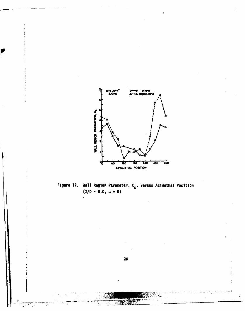
17. Wall Region Parameter, C., Versus Azimuthal Position

(Z/D * 6.0, w * 0) . . . . . . . .. . . . . 26

•7 •

! ,' ,. - ,,: , ," * '' - - -

I. INTRODUCTION

The U.S. Army Ballistic Research Laboratory is interested in theboundary layer development on yawed, spinning slender bodies of revolu-tion for application to the design of artillery projectiles in generaland for gaining further knowledge of the Magnus effect in particular.Reference I presents some experimental evidence showing the significanteffect that the boundary layer configuration has on the agnus forceexperienced by a yawed, spinning body of revolution as well as adiscussion of the influence of Magnus on the aerodynamic stability ofa spin stabilized projectile. Turbulent boundary layer developmentover non-spinning bodies of revolution is also of interest to the Amyin the aerodynamics of missiles.

Recent advances in computational fluid dynamics have resulted inincreased effort toward computation of three dimensional boundary layerdevelopment. References 2-5 report three dimensional, lasinar andturbulent compressible boundary layer computations for bodies of revolu-tion. Comparisons of the computations to experimental boundary layerprofile data have indicated encouraging agreement with the experimentaldata. This indicates that the numerical techniques are working well;however, comparisons to detailed profile data have only been made forcone models. Comparisons to cone data do not test the computationtechnique's ability to cope with effects such as longitudinal pressuregradient or changes in wall curvature. Experimental data for comparisonto theoretical computations of three dimensional compressible turbulentboundary layer development available in the literature are extremely

1. W. B. Stuvek, "Boundary-Layer Distortion on a Spinning Cone," AAAJonal Vol. 11, No. 3, ?4meh 1973, pp. 39&-396.

2. T. C. Lin and S. G. Rubin, A o-Loyer Model for Coupled 2reeDimensional Viscous and Dnvisoid Fto, Caoulations, 0 AWG Paper No.75-853, presented at the AM Fluid and Plasma Drios Conferenoe,Hartford, Connecticut, June 1976.

3. J. C. Adown, Jr., "Finite-Difference Analysis of the Three-Dimensional TurbuZent Boundary Layer on a Sharp Cone at Angle ofAtta k in a Supersonio FZmOU" AXM Paper No. 72-186, presented atthe AIAA 10th Aerospaoe Sciences Meeting, San Diego, California,January 1972.

4. H. A. DLyer and B. R. Sanders, " nu FMorc, o0n Spinning Supersoniccones--Port r: Th BoWdWry Lyer," AZ4 J z Vol. 14, No. 4,April 1076, pp. 49S-604.

5. J. N. Barris, "An kplioit Finite-Diffe ence Proodre for Solvingthe Three-Dimensional Camw@e.aile Laninar, 2'vaitiomal, and2urbulent Dosinday-Lazjer NquUationef NASA SP-847, March 1975,pp. 19-40.

7

A- ____ ___

, :. ,v

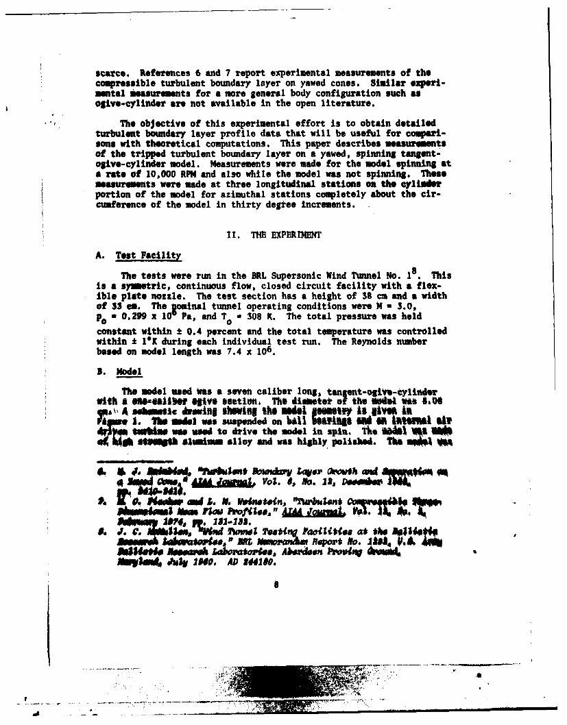
scarce. References 6 and 7 report experimental measurements of thecompressible turbulent boundary layer on yawed cones. Similar oxperi-mental measurements for a more general body configuration such asolive-cylinder are not available in the open literature.

The objective of this experimental effort is to obtain detailedturbulent boundary layer profile date that will be useful for compari-sons with theoretical computations. This paper describes measurementsof the tripped turbulent boundary layer on a yawed, spinning tangent-olive-cylinder model. Measurements were made for the model spinning ata rate of 10,000 RPM and also while the model was not spinning. Thesemeasureamts were made at three longitudinal stations on the cylinderportion of the model for azimuthal stations completely about the cir-cumference of the model in thirty degree increments.

II. THE EXPERIMENT

A. Test Facility

The tests were run in the BRL Supersonic Wind Tunnel No. I8. Thisis a symetric, continuous flow, closed circuit facility with a flex-Ible plate nozzle. The test section has a height of 38 cm and a widthof 33 ea. The pominal tunnel operating conditions were M a 3.0,Po a 0.299 x 10' Pa, and T 0a 308 K. The total pressure was held

constant within 1 0.4 percent and the total temperature was controlledwithin i I1K during each individual test run. The Reynolds numberbased on model length was 7.4 x 106.

3. Model

The msdel used Was a seven caliber long, tangent-oive-cylioderwith a NOf-la IOM O8#1" Ietion, The dimbetet of the ibdol fs 5,0

A sdeMic JnilfA SIMANI thl dMM 1UUil is give ilklaw"1. bmdel was suspended on 1,11 b"ihi6 aim a Utuiiul at

upta. a used to drive the model in spin. Te em V*IV Oa=1A imima alloy and was highly polished. Te

~ Sb #. ftuftten A4. * swwv Laywov chfwh Ow I ~a 11104rot. 00 NO. 18, ,oemuii 4nt M,,,

P. 0 sar Omd 1. . NOO~~ %rba4n*t 9 emf. Pa'of1.. ," MWOi too,

WasaU. a wZft aoiU epor go .J f4 eh*U0.* *seem* ZL~ais Abvdeen PvoV 6wasi4MiNy8.4 4u3V IMP0. AD 244100.

dynamically balanced to a tolerance of 2.x10 "4 (Nm). A boundary layertrip consisting of a 0.64 ca wide band of #80 sand grit was placed 2.5cu from the tip of the model.

C. Survey Mechanism

The survey mechanism, shown installed with the model in Figure 2,was designed to drive the probe perpendicular to the axis of the nodel.The probe is positioned by a can that is rotated using an electricmotor mounted within the angle-of-attack crescent. Since the surveymechanism is attached to the angle of attack crescent, the probe isdriven perpendicular to the axis of the model for any angle of attacksetting. The azimuthal position is determined by selecting predrilledmounting holes placed at 30* increments. The number of azimuthalposition changes was kept to a minimu by obtaining data at positiveand negative angles of attack.

The survey mechanism was calibrated by using a dial indicator toindicate the displacment of the probe support in thousandths of aninch to establish a table of displacement versus electrical outputsignal from the probe drive mechanism. In the data reduction procedure

:.divided differnc inte lation was used to determine the y position

for a given electrical signal. The coordinate system is indicated in

D. Test Procedure

Total head surveys were made of the boundary layer at three longi-tudinal positioas along the cylinder portion of the model for an angleof attack of 4, N a 3, mnd for spin rates of zero and 10,000 RPM.The total head probe used had a flattened tip. The probe tip had anopening of 0.076 m with a lip thickness of 0.025 sm and was 2.5 s-in width. The probe was positioned to measure the pressure alonglines parallel to the model axis. A spark shadowgraph showing the modelwith the total head probe positioned beyond the boundary layer is shownin Figure 4.

The surveys were mde by starting the measurements well beyond theedge of the boundary layer--at y - 1.25 ca whereas the largest 6 was

about 0.65 c. The pressure signal from the total head probe wasmeasured using a strain gage transducer that was calibrated within± 0.25 percent of its full scale range--0-25 psi (0-0.172 x 100 Pa).Measurements were made while holding the probe in a fixed positionafter allowing approximately thirty seconds for the pressure signal tostabilize. The position of the model surface was detected by electri-cal signal when the probe contacted the surface of the non-spinningmodel. Immediately following the survey for the model not spinning,the model was spun to 10,000 RPM and another survey made again startingfrom well beyond the outer edge of the viscous region. The model spinrate was held constant within ± SO RPM during the survey using an

9

JUI

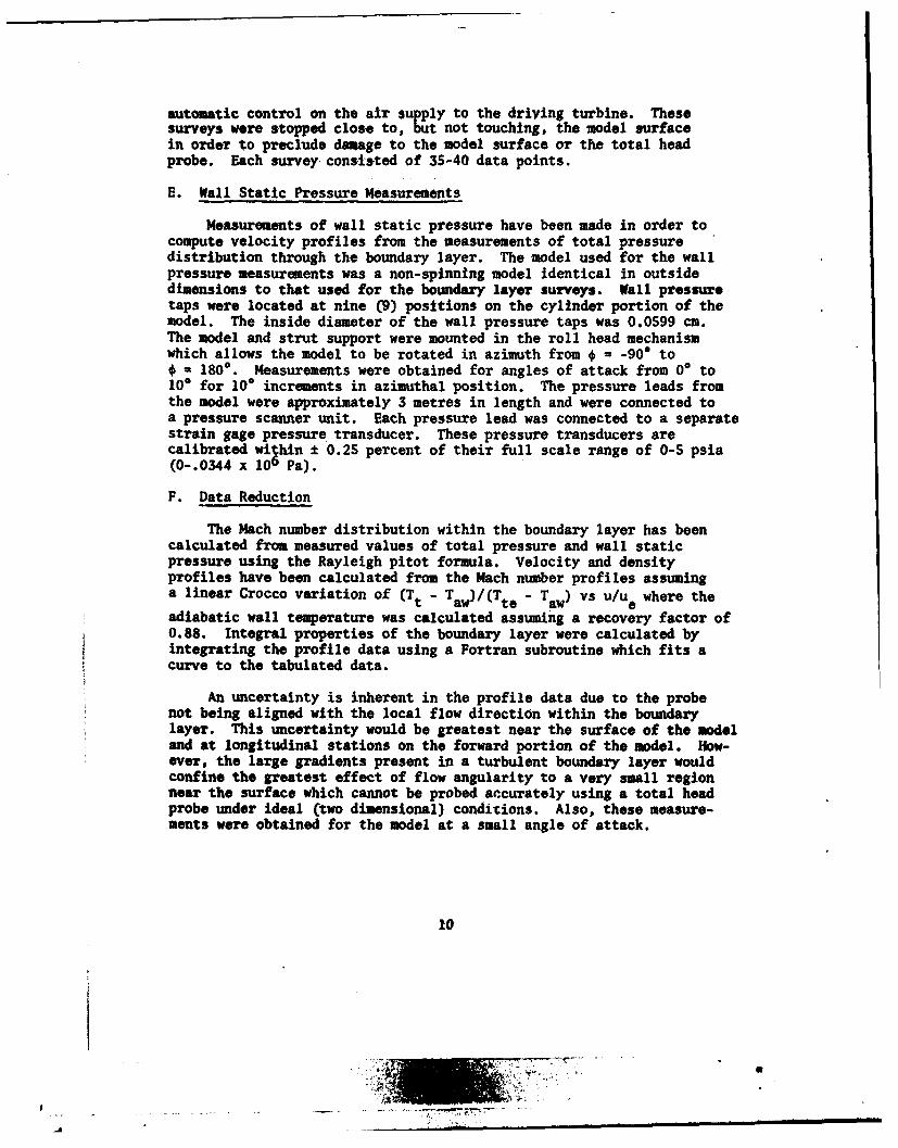
automatic control on the air supply to the driving turbine. Thesesurveys were stopped close to, but not touching, the model surfacein order to preclude damage to the model surface or the total headprobe. Each survey consisted of 35-40 data points.

E. Wall Static Pressure Measurements

Measurements of wall static pressure have been made in order tocompute velocity profiles from the measurements of total pressuredistribution through the boundary layer. The model used for the wallpressure measurements was a non-spinning model identical in outsidedimensions to that used for the boundary layer surveys. Wall pressuretaps were located at nine (9) positions on the cylinder portion of themodel. The inside diameter of the wall pressure taps was 0.0599 cm.The model and strut support were mounted in the roll head mechanismwhich allows the model to be rotated in azimuth from 0 = -90* to* - 1800. Measurements were obtained for angles of attack from 0* to10* for 10* increments in azimuthal position. The pressure leads fromthe model were approximately 3 metres in length and were connected toa pressure scanner unit. Each pressure lead was connected to a separatestrain gage pressure transducer. These pressure transducers arecalibrated within ± 0.25 percent of their full scale range of 0-5 psia(0-.0344 x 106 Pa).

F. Data Reduction

The Mach number distribution within the boundary layer has beencalculated from measured values of total pressure and wall staticpressure using the Rayleigh pitot formula. Velocity and densityprofiles have been calculated from the Mach number profiles assuminga linear Crocco variation of CTt - Taw)/(Tte - Taw) vs u/u where the

adiabatic wall temperature was calculated assuming a recovery factor of0.88. Integral properties of the boundary layer were calculated byintegrating the profile data using a Fortran subroutine which fits acurve to the tabulated data.

An uncertainty is inherent in the profile data due to the probenot being aligned with the local flow direction within the boundarylayer. This uncertainty would be greatest near the surface of the modeland at longitudinal stations on the forward portion of the model. How-ever, the large gradients present in a turbulent boundary layer wouldconfine the greatest effect of flow angularity to a very small regionnear the surface which cannot be probed accurately using a total headprobe under ideal (two dimensional) conditions. Also, these measure-ments were obtained for the model at a small angle of attack.

10

-J

III. DISCUSSION OF THE RESULTS

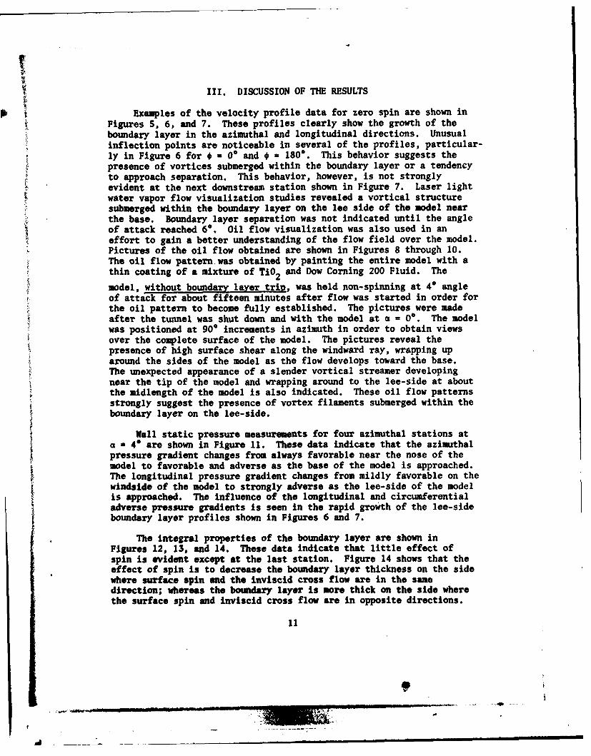
Examples of the velocity profile data for zero spin are shown inFigures 5, 6, and 7. These profiles clearly show the growth of theboundary layer in the azimuthal and longitudinal directions. Unusualinflection points are noticeable in several of the profiles, particular-ly in Figure 6 for 0 =0 e and =180. This behavior suggests thepresence of vortices submerged within the boundary layer or a tendencyto approach separation. This behavior, however, is not stronglyevident at the next downstream station shown in Figure 7. Laser lightwater vapor flow visualization studies revealed a vortical structuresubmerged within the boundary layer on the lee side of the model nearthe base. Boundary layer separation was not indicated until the angleof attack reached 60. Oil flow visualization was also used in aneffort to gain a better understanding of the flow field over the model.Pictures of the oil flow obtained are shown in Figures 8 through 10.The oil flow pattern was obtained by painting the entire model with athin coating of a mixture of TiO2 and Dow Corning 200 Fluid. The

model, without boundary layer trip, was held non-spinning at 40 angleof attack for about fifteen minutes after flow was started in order forthe oil pattern to become fully established. The pictures were madeafter the tunnel was shut down and with the model at a = 0*. The modelwas positioned at 90* increments in azimuth in order to obtain viewsover the complete surface of the model. The pictures reveal thepresence of high surface shear along the windward ray, wrapping uparound the sides of the model as the flow develops toward the base.The unexpected appearance of a slender vortical streamer developingnear the tip of the model and wrapping around to the lee-side at aboutthe midlength of the model is also indicated. These oil flow patternsstrongly suggest the presence of vortex filaments submerged within theboundary layer on the lee-side.

Wall static pressure measurements for four azimuthal stations ata a 40 are shown in Figure 11. These data indicate that the azimuthalpressure gradient changes from always favorable near the nose of themodel to favorable and adverse as the base of the model is approached.The longitudinal pressure gradient changes from mildly favorable on thewindside of the model to strongly adverse as the lee-side of the modelis approached. The influence of the longitudinal and circumferentialadverse pressure gradients is seen in the rapid growth of the lee-sideboundary layer profiles shown in Figures 6 and 7.

The integral properties of the boundary layer are shown inFigures 12, 13, and 14. These data indicate that little effect ofspin is evident except at the last station. Figure 14 shows that theeffect of spin is to decrease the boundary layer thickness on the sidewhere surface spin and the inviscid cross flow are in the samedirection; whereas the bomdary layer is more thick on the side wherethe surface spin and inviscid cross flow are in opposite directions.

11

The growth of the boundary layer in the circumferential and longitudinaldirections is shown in the plots of 6* and e. The plots of the formfactor, H, indicate little effect of longitudinal or circumferentialstation. The form factor is, however, consistently greater for thespinning model.

IV. LAW OF THE WALL ANALYSIS

A. Profile Characterization

An attempt has been made to gain additional information about thecharacteristics of the measured velocity profiles using "law of thewall" and "law of the wake" turbulent boundary layer concepts. Theprocedure used is based on the method proposed in reference 9 wherea least square fitting technique is employed to determine certainprofile parametgrs. The form of the assumed profile is based on thework of Coles' in incompressible flow in which the boundary layeris found to have a wall region in which the velocity is dependent on avelocity scale, us, and a length scale, v /us, and a wake region which

is also dependent on us but the length scale is a boundary layer

thickness, 6 s. The following functional relationship was used in thedata reduction:

u/us = In (usy/v ) + Cs + 2 Rs sin2 (wy/26) . ()

law of the wall law of the wake

Compressibility effects are accounted for, f least approximately,using the results of the Prandtl-Van Driest" mixing length analysisin which the compressible flow velocity, u, is transformed into anequivalent incompressible form through the relation

9. J. E. Danberg, "A Re-evaluation of Zero Pressure Gradient Comree-eibte Turbulent Boundary Layer Measuremente," Proceedings CP-93,AGARD Fluid Dyn ice Specialists Meeting on 'Turbulent Shear lFa',1971.

10. D. R. Cole, "The Law of the Wake in TurbuZent Boundary Layere,"Journal of Fluid Meohanic VoW. 1, Part 2, 1956, pp. 191-226; aleo,ae D. R. Colee and R. A. Hirst, "Prooeedings AFOSR-IFP-StanfordConference on Coputation of Turbulent Boundary Layere--1968,"Vot. II, pp. 1-45.

11. F. R. Van Drieet, "TurbuZent Bound=ay Layers in CompreeibleFluids," Journal of Aeronautical Sciene. Vol. 18, No. 3, 1951,pp. 145-160.

12

,, Wffi

U

fu rplio du (2)

which is evaluated numerically from the measured Mach number profilesand assuming: (1) constant pressure across the boundary layer,(2) perfect gas equation of state, (3) adiabatic relationship betweenMach number, total and static temperature, and (4) the Crocco tempera-ture-velocity equation

2crt T)/(Tte - T ) - + (1 -0)(u/U).. C3)

1B (=Taw ) (Tt -T)

with a constant recovery factor of .89 used in evaluating the adiabatic

wall temperature.

In equation (1) there are four parameters; us, Cs, s3 , and 6s

which are determined so as to minimize the rms deviation between theprofile measurements and the analytical curve. It should be notedthat the form of the "law of the wall" used here is not valid in thelaminar sublayer region near the wall. Data close to the wall whichsystematically deviate from the semilogarithmic relation are omittedfrom the fitting procedure. The equation is also not valid when thevelocity becomes uniform at the edge of the boundary layer. Only datacorresponding to y values less than 8 are used in the curve fitting,where 8 is defined as the value of y at which the derivative of equation

(1), that is du/dy, is zero. The boundary layer thickness, 8, istypically ten percent larger than 8s .

The more conventional form of equation (1), for exaple as usedby Coles 1 0 , is related to equation (1) when

US - UT/IK (4)

where K - Prandtl's mixing length constant

uT - wall shear velocity a 67Pq

As a consequence the usual constant in the logarithmic wall law isrelated to Cs by

13

C s CK + In K (5)

The change in definition of these two parameters is desirable for thepresent purposes because K cannot be determined solely from velocityprofile data unless accurate data in the laminar sublayor is obtained.However, if K is assumed known (K - .4 approximately) then equation (4)may be used to determine the wall shear stress.

Equation (1) is found to adequately describe a wide range of two-dimensional turbulent boundary layer measurements except, of course,in the laminar sublayer. Most two-dimensional profiles can berepresented in this way with a root-mean-square deviation of less than

t .03 in ;/u s . This corresponds to about t .3% of the maximum flow

velocity at the edge of the boundary layer which is approximately theerror expected in the transducers used for the pressure measurements.The fit of the three-dimensional boundary layers considered here wastypically the same with the maxium rms deviation of .09%. Figure 15illustrates the quality of the fit obtained with the present data.The figure shows the variation of the velocity profiles with azimuthalposition for the most rearward station (6 calibers from the nose) onthe non-spinning model. The thickening of the boundary layer on theleeward side (1800) is evident as well as a significant increase in thesize of the wake region of the profile. The profiles obtained on thespinning model at 10,000 RPM are essentially the same as for the non-spinning case.

B. Azimuthal Distribution of Profile Parameters

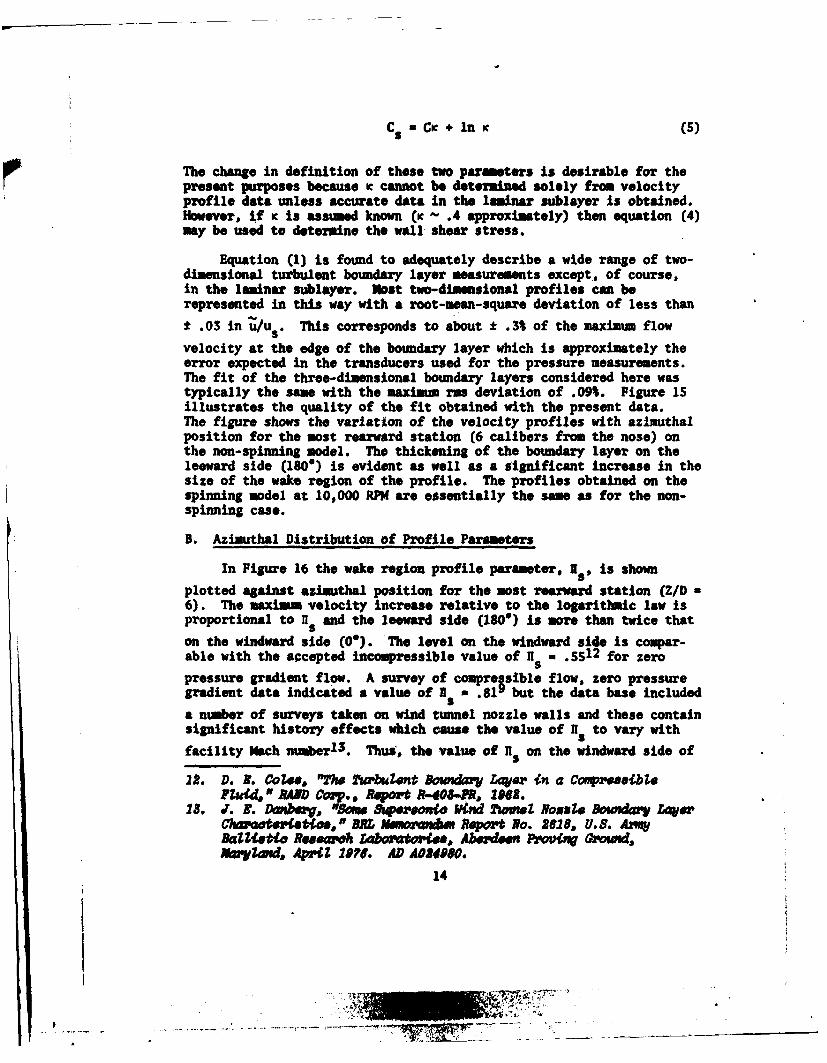
In Figure 16 the wake region profile parameter, I., is shown

plotted against azimuthal position for the most rearward station (Z/D6). The maxima velocity increase relative to the logarithmic law isproportional to f 5 and the leeward side (180") is more than twice thaton the windward side (0"). The level on the windward side is compar-able with the accepted incompressible value of 9 s = "S12 for zero

pressure gradient flow. A survey of compreisible flow, zero pressuregradient data indicated a value of 1 a .811 but the data base included

a number of surveys taken on wind tunnel nozzle walls and these containsignificant history effects which cause the value of a s to vary with

facility Mach number 1 3 . Thus, the value of Ns on the windward side of

22. D. f. Cole, "Me Tk'mbulent Now Vy ,Ler in a Conaess*,elI" RAID Coy.. *e Rpozt R-,0P, 196.

1s. J. I. Dmberf' W80" "Sam e rreox Vd 2'WMeZ lOXZS l owidow LCowtevtatoe,"f DRL Memoztanm Report No. 2618, U.S. A2"wBaZUeto RmeeazeA Laboz'tovies, Aberdeen frovn Growad,Mozyl.'d Aprit 20?I. AD MUMDIO

14

the model is essentially that of a zero pressure gradient, two dimen-sional boundary layer. On the leeward side I is more characteristic

of an adverse pressure gradient situation. In addition to the variationof 115 with azimuthal angle, there is also a small but consistent effectof spin. At 10,000 RPM the curves are slightly displaced in thedirection of rotation.

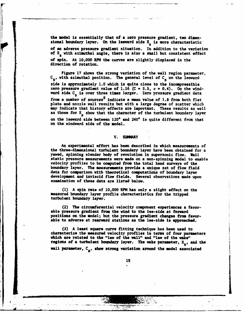
Figure 17 shows the strong variation of the wall region parameter,C39 with azimuthal position. The general level of C5 on the leeward

side is approximately 1.0 which is quite close to the incompressiblezero pressure gradient value of 1.16 (C - 5.5, K - 0.4). On the wind-ward side Cs is over three times larger. Zero pressure gradient data

from a number of sources9 indicate a mean value of 1.8 from both flatplate and nozzle wall results but with a large degree of scatter whichmay indicate that history effects are important. These results as wellas those for 1s show that the character of the turbulent boundary layer

on the leeward side between 1200 and 240 ° is quite different from thaton the windward side of the model.

V. SUMARY

An experimental effort has been described in which measurements ofthe three-dimensional turbulent boundary layer have been obtained for ayawed, spinning slender body of revolution in supersonic flow. Wallstatic pressure measurements were made on a non-spinning model to enablevelocity profiles to be computed from the total head surveys of theboundary layer. The measurements provide a unique set of flow fielddata for comparison with theoretical computations of boundary layerdevelopment and inviscid flow fields. Several observations made uponexamination of these data are listed below.

(1) A spin rate of 10,000 RPM has only a slight effect on themeasured boundary layer profile characteristics for the trippedturbulent boundary layer.

(2) The circumferential velocity component experiences a favor-able pressure gradient from the wind to the lee-side at forwardpositions on the model; but the pressure gradient changes from favor-able to adverse at rearward stations as the lee-side is approached.

(3) A least square curve fitting technique has been used tocharacterize the masured velocity profiles in terms of four parameterswhich are related to the "law of the wall" and "law of the wake"regions of a turbulent boudary layer. The wake parameter, I., and the

wall parameter, Cs, show strong variation around the model associated

1s

M---------------------------

rv

with the, effects of angle of attack. one effect of spin rate is foundto be a shift in th. wak. profile Parameter distribution In the

directibm of spin.

16

- - . I

REFERENCES

1. W. B. Sturek, "Boundary-Layer Distortion on a Spinning Cone,"AZAA Jo'urnat, Vol. 11, No. 3, March 1973, pp. 395-396.

2. T. C. Lin and S. G. Rubin, "A Two-Layer Model for Coupled ThreeDimensional Viscous and Inviscid Plow Calculations," AIM PaperNo. 75-853, presented at the AIM Fluid and Plasma DynamicsConference, Hartford, Connecticut, June 1975.

3. J. C. Adams, Jr., "Finite-Difference Analysis of the Three-Dimensional Tubulent Boundary Layer on a Sharp Cone at Angle ofAttack in a Supersonic Flow," AIM Paper No. 72-186, presented atthe AIAA 10th Aerospace Sciences Meeting, San Diego, California,January 1972.

4. H. A. Dwyer and B. R. Sanders, "Magnus Forces on Spinning Super-sonic Cones--Part I: The Boundary Layer," AIAA Jou2'lZ, Vol. 14,No. 4, April 1976, pp. 498-504.

S. J. E. Harris, "An Implicit Finite-Difference Procedure for Solvingthe Three-Dimensional Compressible Laminar, Transitional, andTurbulent Boundary-Layer Equations," NASA SP-347, March 1975,pp. 19-40.

6. W. J. Rainbird, "Turbulent Boundary Layer Growth and Separation ona Yawed Cone," A'AA JournaL, Vol. 6, No. 12, December 1968,pp. 2410-2416.

7. M. C. Fischer and L. M. Weinstein, "Turbulent Compressible Three-Dimensional Mean Flow Profiles," ArAA Journal, Vol. 12, No. 2,February 1974, pp. 131-132.

8. J. C. McMullen, "Wind Tunnel Testing Facilities at the BallisticResearch Laboratories," BRL Memorandum Report No. 1292, U.S. ArmyBallistic Research Laboratories, Aberdeen Proving Ground, Maryland,July 1960. -AD 244180.

9. J. E. Danberg, "A Re-evaluation of Zero Pressure Gradient Compres-sible Turbulent Boundary Layer Measurements," Proceedings CP-93,AGARD Fluid Dynamics Specialists Meeting on 'Turbulent ShearFlows', 1971.

10. D. E. Coles, The Law of the Wake in Turbulent Boundary Layers,"Jrounal of M iddAimhoe, Vol. 1, Part 2, 1956, pp. 191-226;also, see D. E. Coles and B. A. Hirst, "Proceedings APOS-IFP-Stanford Conference on Computation of Turbulent Boundary Layers--1968," Vol. II, pp. 1-45.

17

CContinued)

11. 1. It. Van Driest, Orutwulet owndary Layers in CoqpressibleFluids," JoMt' of Awowatu &idnao.j Vol. 18, No. 3, 19SI,pp. 14S-160.

12. D. B. Coles, The Tuflemiet oumdary Layer in a Compressible Fluid,"RAND Corp., Report I-403-PR, 1962.

13. J. E. Danborg, "Sam Suprsonic Wind Tunnel Nozzle Boundary LayerCharacteristics," IL Nnorsaam Report No. 2618, U.$. ArmyBallistic Aesearh Ls res, Absdm Prwla Gnmrd,Maryland, April 1976. AD A0249.

IKS1a2

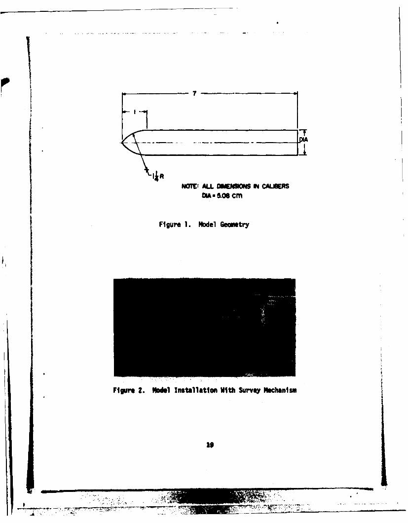
N=T: &LL ONENSM~d IN CAUKASCIA. a506 CM

Figure 1. Model Geometry

Figure 2. Model Installation With Survey Mechanism

19i

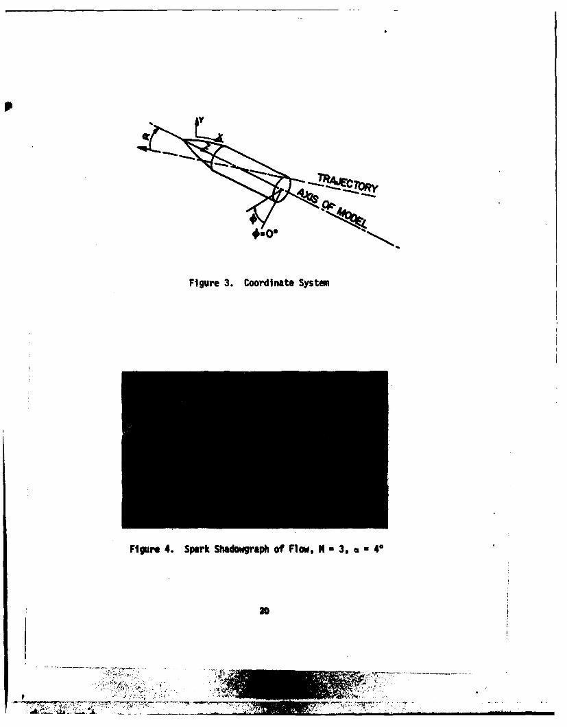
Figure 3. Coordinate System

Figure 4. Spark Shadowgraph of Flow, N -3, 40

20

04

03

O) ' . •

Y/L

AI :I /I /..' 3

OF k " . , b. " - " . , ,,*- I .

0 02 04 04 O0 I0 0 '0 10 .0 10 I0

U/u e

Figure 5. Velocity Profiles, M = 3, a , 40, Z/D = 3.0,Zero Spin

AZMLP00OV 4 ' 5' E0 0 20 0 0

04 AZIMTHA FOfIk . 3* . 9, 10 5.

Y/L £10IA I011110O. 2/0.4 .

I 1 .

f

u/u0

Figure 6. Velocity Profiles, M = 3, a 40, Z/D = 4.5,Zero Sptn

AZIMUTHAL POJTION, -0 30 GOP ow 120' o0 6W

0,4 .

Y/L . ..

Y/L 1 AXIAL POWV.;. /• 60

0If

1 0.2 04 0 I o to .0

U/U.

Figure 7. Velocity Profiles, M 3, - 40, Z/D - 6.0,Zero Spin

21

Figure 8. 0il Flow Visualization, NM 3, ei=40,, 0 00

Figure 9. 011 Flow Visualization, M 3, a 4%, o 900

Figure 10. Oil Flow Visualization, M 3, *40, * 1800

22

M-3, az4 °

1.0 . ..- , . - _ _ . -. - . .- ,

.9 .**-- -- - - a-.9 . 0- n oJ O

Pw x6 00 - -- 0~00PO S'P~ .8 --

17 41120 ,/-

.60 * * * * I I I I I I i £ I i I I I I I I I I I I I I

0 I 2 3 4 5 6 7Z/D

Figure 11. Wall Static Pressure Distribution, M - 3, a - 40

CONIG 5 0 0 RPM6- M/3.•40 -- 0,000 RPM

Z/023

H L 5 0 0O~000

.04rO o . -

.02m

.20

.10 a~c% f-- "--0

00 60 120 lio 240 300 360

AZMJTHAL POSITION, €OWIN¢ CWOS9FLOW-SW AM: SMN =

Figure 12. Integral Properties of the Boundary Layer, Z/D 3.0

23

CONFIG 4 0 0 RPM

6 Mc., a-40 . 10.000 RPM CONFIG 3 0 0 RPMZ/,4 M,3, CI,4" - 10,000 RPMZ/D,6

0

4L

08-OBa

0600-

04 9.- Q ,.cm %

Ocm > * 04

02 0'S I -* -0-

20 320

- - o,-- " *0

02m -'"-"° O "% .0 , o- ' ° o-..,0,30 r " 3

8 ,cm '0 , , , 20 -

15 ICY 0 ,cm - -09

10, A 10 l , . -0

60 10IUTH 24 0360 0 60 120 IwO 240 300 360AZMLUTHAL POSITION, AZIMUTHAL PoSI~oNo

INVISCIo CROSSFLOW • P S""

SURFACE SPIN -. -- INVISCIO CROSSFLOWSURFACE SPIN

Figure 13. Integral Properties of Figure 14. Integral Properties ofthe Boundary Layer, the Boundary Layer,Z/D = 4.5 Z/D = 6.0

24

14 - ,.r* V V* ~ ~ ** . u v v.

12 - 0-18.10-

6-

4 60

2- 0934

0 Z/ -60w0

0 60 A.20 M0 a4 300 360I.

Figure 1. WaelRegion Prameter, in Versus Azmal oition

(/D 6.0 w 0)

Me ,G4* -- 0 25P

3 N~

AA,

2 26

=7 p 77( *77

LIST OF SYNDOLS

C5 law of the wall profile parameter

D diameter of del, 5.06 cm

L reference length, 2.S4 cm

T temperature

u longitudinal velocity composent

u a velocity scale parameter

u wal shear velocity = (TW/PW)

u transformed velocity [see equation (2)]

y coordinate normal to surface

0 (Taw- Tw)/(Tt - Tw)

6 boundary layer thickness

a 8 boundary layer thickness parameter

K Prandtl mixing length constant - 0.4

V kinematic viscosity

11 law of the wake profile parameter

p density

Subscripts

aw adiabatic wall

• edge of the bounday layer

t total temperature

w wall

27

7771'

DISTRIBUTION LIST

No. of No. ofCopies Omanization Copies O zation

12 Commnder 2 commmnderDefense Documentation Center US Army Nobility EquipmentAT7m: DDC-TCA Research 4 Developmnt ComandCmerofn Station ATTN: Tech Docu Con, Bldg. 315Alexandria, VA 22314 DRSNE-RZT

Port Belvoir, VA 220601 Commander

US Army Materiel Development 1 Camuderand Readiness Conamnd US. Army Armment Commnd

ATN: DRVDNA-ST Rock Island, IL 612025001 Eisenhower AvenueAlexandria, VA 22333 3 Commander

US Army Picatinny ArsenalConAder ATNl: SARPA-PR-S-AUS Army Aviation Systems Mr. D. Mertz

Command Mr. E. FalkowskiATIW: DRSAV-E Mr. A. Loeb12th and Spruce Streets Dover, NJ 07801St. Louis, MD 63166Director Co ne

1 Commander

I Director US Army Jefferson ProvingUS Army Air Nobility Research Grodand Developmt Laboratory AT d: STEJP-TD-DAMs Research Center , Mdison, IN 472S0

Noffett Field, CA 9403d

SCommader1 I Commder

US ArmY EMler Comand US Army Hary Diamond LabsUS Ary Elctroncs CmmdAITM: ' DRXb0-TIATTM: DRSEL-RDL 2800 Powder Miln RoadFort MNsiouth, NJ 07703 Adelphi, ND 20783

4 Commnder IDirectorUS Army Missile Commnd US Amy TRADOC SystemATTN: DRSNI-R Analysis Activity

DRSMI -RI K ATFN: ATAA-SAMr. R. Deep White Sands Missile RangeMr. R. Becht 1M 88002Dr. D. Spring

Redstone Arsenal, AL 35809 CommaderUS Army Research Office

1 Commander P. 0. Box 12211US Army Tank Automtive Research Triangle Park

Development Command NC 27709ATTN: DTA-lULWarren, MI 480N

7"7

L~: , . , : ' : i :,- , • .

p " f

DISTRIBUTION LIST

No. of No. ofcopies Organization Copies Organization

2 Commnder 2 Princeton UniversityDavid W. Taylor Naval Ship James Forrestal Research Center

Research 4 Development Ctr Gas Dynamics LaboratoryATTN: Dr. S. de los Santos ATIi: Prof. S. Bogdonoff

Mr. Stanley Gottlieb Prof. I. VasBethesda, M) 20084 Princeton, NJ 08540

1 Commander 1 University of CaliforniaUS Naval Surface Weapons Con Department of Mechanical EngA1M: Dr. T. Clare, Code DK20 ATIN: Prof. H4. A. DwyerDhlgren, VA 22448 Davis, CA 95616

4 Commander 1 University of DelawareUS Naval Surface Weapons Con Mechanical and AerospaceATTN: Code 312, S. Hastings Engineering Department

Code 313, Mr. R. Lee ATTN: Dr. J. E. DanbergMr. V. Yanta Newark, DE 19711Mr. R. Voisinet

Silver Spring, ND 20910 2 University of VirginiaDept of Aerospace Engineering

2 Director and Engineering PhysicsNational Aeronautics and ATTN: Prof. I. Jacobson

Space Administration Prof. J. B. MortonLangley Research Center Charlottesville, VA 22904ATTN: HS 185, Tech Lib

MS 161, D. Bushnell Aberdeen Proving GroundLangley StationHampton, VA 23365 Marine Corps La Ofc

Dir, USANSAA1 Douglas Aircraft Company

McDonnell Douglas CorpATFN: Dr. Tuncer Cebeci3855 Lakevood BoulevardLong Beach, CA 90801

I Sadia LaboratoriesATTN: Dr. F. G. BlottnerP. 0. Box 5800Albuquerque, I 8711S

30

2 LA