Report Iceberg Flux and Climate Changesbruneau/research/publications/2008cis.pdf · Report Iceberg Flux and Climate Change FOR THE CANADIAN ICE SERVICE JUNE 2007 - MARCH 2008 Submitted

Report Iceberg Flux and Climate Change

FOR THE CANADIAN ICE SERVICE JUNE 2007 - MARCH 2008

Submitted to:

Canadian Ice Service Environment Canada

373 Sussex Drive, Block E Ottawa, ON

K1A 0H3 Scientific Authority:

Tom Carrieres

Submitted by:

Dr. S. E. Bruneau

CBERG Consulting Services 13 Darcy St., St. John’s NL, Canada, A1A 5B9

Ph 709 722-6542

CCS 01-08 March 31, 2008 St. John’s, NL. Can

Proprietary Notice

Please Note that all information, discussions, concepts, ideas and recommendations contained in this document are proprietary to the client and the author. No part of this document may be communicated to any individual other that the intended recipient without prior permission from the author.

ii

Iceberg Flux and Climate Change Dr. S. E. Bruneau

TABLE OF CONTENTS

PREAMBLE .................................................................................................................... 1

BACKGROUND.............................................................................................................. 1

ICEBERG MODEL INSTALLATION AND CHECKS...................................................... 2

Model Implementation .................................................................................................. 2

Extension of Sensitivity Studies ................................................................................... 5

Model Operability for This Study .................................................................................. 7

Localberg Code Experiment and ANOVA .................................................................... 8

ICEBERG FLUX PARAMETRIC STUDY...................................................................... 11

Solar Influence ........................................................................................................... 12

NAO Influence............................................................................................................ 14

Sea Ice Influence ....................................................................................................... 16

Apparent Modal Behaviour......................................................................................... 17

ICEBERG MODELING STRATEGIES FOR CLIMATE CHANGE................................ 19

ICEBERG DETERIORATION FIELD WORK - JUNE 2007, ST.JOHN’S ..................... 22

Summary of Calving Events at Signal Hill .................................................................. 23

Analysis and Discussion............................................................................................. 25

1


PREAMBLE This report details the work by Dr. Stephen E. Bruneau, Assistant Professor of Civil Engineering at Memorial University. Dr. Bruneau in his capacity as a contracting consultant entered into a Short Form Service Contract with AES Ice Centre, Tom Carriers Scientific Authority. The work was carried out between June of 2007 (earliest field component) and March of 2008 (final analytical work). Dr Bruneau wishes to acknowledge support from colleagues Dr. Greg Crocker and Mr Tom Carriers and also the contributions of Memorial students Mr Eugene Manning, Mr Evan Martin and Mr Kris Rogers for their technical assistance. BACKGROUND The Canadian Ice Service (CIS) provides sea ice and iceberg information to governmental and industrial users on Canada’s east coast and in the Canadian Arctic. Hydrocarbon exploration and development activities on the Grand Banks of Newfoundland have resulted in an increased demand for iceberg information in this region. In response to this user requirement, and to further meet its mandate of environmental protection and the safety of lives at sea, the CIS is actively developing improved iceberg products and services. The CIS iceberg drift and deterioration model is used operationally to forecast and now-cast iceberg positions. It can also be used to investigate iceberg climatology. It is generally accepted that warming and other changes to the global climate system will continue through the next several decades. Changes to air and sea temperatures, currents, wind fields, and storm frequency, severity and tracking will all act to change the drift patterns of icebergs. The recent dearth of icebergs near to shore along Newfoundland’s northeast coast may be evidence that this is already happening. It is not presently known what the most important factors will be in controlling changes to iceberg drift patterns, how drift patterns might be changed, and how the flux of icebergs to the hydrocarbon developments on the northern Grand Banks will be affected. In this study the CIS iceberg drift and deterioration model will be used to conduct parametric studies of the effects of plausible changes to met-ocean conditions on the drift patterns and flux of icebergs from Davis Strait to the northeast coast of Newfoundland and the northern Grand Banks.

2


ICEBERG MODEL INSTALLATION AND CHECKS This section of the report describes action items associated with installation, checking and the configuration of the model to facilitate efficient parametric investigations of iceberg flux and climate change. Specifically described are:

1. model implementation and checks for validation of version correctness 2. model operability for the purposes of studying Iceberg Flux and Climate Change 3. model input versus output statistical analysis for the purpose of prioritizing input

parameters in the study of Iceberg Flux and Climate Change Model Implementation The CIS iceberg model called localberg was obtained by the consultant through the procurement of a “Single System Licence For Local Iceberg Drift Software” agreement with a third party - the National Research Council, Canada (NRC). For proprietary reasons the version provided for evaluation was of a non-readable executable form and therefore could only be run exclusively as-is. Subsequent to the award of this contract an important publication became available from those credited for the CIS-NRC Local Iceberg Drift Model. The work is entitled “An Operational Iceberg Deterioration Model” (Kubat et al., ISOPE 2007), and in combination with an earlier publication “Determination of Iceberg Draft, Mass and Cross-Sectional Areas” (Barker et al ISOPE 2004) most of the relevant physics for both the drift and the deterioration components of localberg are explained. Kubat et al (2007) describes the formulation for the iceberg deterioration component of localberg exclusively and importantly, the paper describes output sensitivity to certain key input parameters. One test case is described for which an aggressive melting scenario is modelled and several but not all input parameters are listed. To validate the version of localberg in hand this singular published test case was replicated for comparison. The test case from Kubat et al, 2007 features the following input data: The resulting decrease in waterline length and mass were plotted versus time. Results showed a length decrease from 100 to 60 m and a mass reduction of 87% after 4 days.

Kubat et al: Test Case in ISOPE 2007

Iceberg waterline length 100 mSea water temp 11.9 CDuration of run 4 daysWind, wave & current deltas noneWave height 2.1 mWave period 8 sWind Velocity 0 m/sCurrent (velocity) 0.5 m/s

3


Utilizing the same input values as listed above and otherwise relying on the default data in the sample input parameter file, the following results were obtained by this author (complete input listing provided below):

This program is for use by: CBERG Consulting Services under licence from NRC-CHC.--------------------------------------------------------

Model Parameters----------------

Run Parameters Initial Iceberg Variables Environmental Forcing PropertiesuserNsteps: 3390 userBergLength: 100.00 userWaterTemp: 11.900 userCdwat: 1.3000userDelt: 120.000 userLong: 55.000000 userWaveHeight: 2.100 userCdair: 1.9000userPrintFreq: 150 userLat: 50.000000 userWavePeriod: 8.000 userRhoice: 910.000

userU: 0.0000 userInitUcurrent: 0.5000 userRhoair: 1.3000userV: 0.0000 userInitVcurrent: 0.5000 userRhowat: 1030.000userTabularGeometry: 0 userInitUwind: 0.0000 userKwater: 0.562000userKeelSailInput: 1 userInitVwind: 0.0000 userKair: 0.024100userKeelDepth: 70.000 userNuwater: 1.7900E-06userSailHeight: 10.000 userNuair: 1.3200E-05

userLatentHeat: 3.3400E+05userAlbedo: 0.7000

Iceberg Mass Loss over 4 days

0

100000

200000

300000

400000

500000

0 24 48 72 96 120

Hours

Ber

g M

ass

(ton

nes)

Iceberg waterline Length Decrease over 4 Days

0

20

40

60

80

100

120

0 24 48 72 96 120

Hours

Ber

g Le

ngth

(m)

4


The resulting output depicted above compares favourably to the output described and plotted in ISOPE. The deterioration clearly follows the same trends and is similar in magnitude; however, the mass reduction recorded by the test case in Kubat et al indicated an 87% decrease whereas the results computed here were just under 80%. The differences may be attributed to invalid assumptions by this author of those input parameters that are not provided in the ISOPE paper. None-the-less it is judged that this test sufficiently proves that the executable model obtained from the NRC is one and the same as that in Kubat et al, and, that it is functioning as intended. Sensitivity studies have been carried out on the operational CIS model and are described in Kubat et al 2007. They were intended to guide in the operational use of the model. Parameters tested were water temperature, iceberg size (waterline length), wind and current velocities and wave height.

5


The results indicated that wave height and water temperature were the most significant independent variables in the model when tested over a natural range of values. Other parameters affected decomposition noticeably but with less severity. Calving intervals were also shown to match reasonably well with field observations. Extension of Sensitivity Studies It is estimated that Greenland produces more than 100 billion tones of iceberg ice annually and that only 5% of this or about 2000 bergs make it through the Davis Strait each year. This implies that the vast majority of icebergs melt entirely within Baffin Bay or adjacent waters. This melting may not occur in a single season but can span several if the iceberg is unable to exit to the south into ice free waters. As will be discussed later in this report it is well established that icebergs do not melt or break up appreciably when locked in sea ice. Sea ice may convey bergs but water temperatures are usually below zero, air temperatures are usually below melting point and wave action is curtailed entirely. Thus icebergs are preserved and transported in sea ice – but not melted. The plot below indicates the average weekly ice coverage of Baffin Bay and also shows the anomalous histogram for the 2007 season. Of note is the extended duration of the ice “free” (25% for this example) period from approximately 7 weeks in an average year to approximately 11 weeks for the 2007 season. Though this change in ice cover is relatively small when stretched out over the entire sea ice year (less than 10% change), it represents a whopping 50% increase in open water exposure to icebergs freed in that period. This sensitivity is illustrated by the following hypothetical deterioration cases as computed using the executable localberg model: If the average open water temperatures of Baffin Bay were 2C and wave height were fixed at 1.5 m with no wind or appreciable currents then an iceberg with a waterline length of 200m and mass of 3.6 million tonnes would take almost 20 weeks to vanish according to the CIS model. Raising temperatures to 4C reduces this to 11

6


weeks. A smaller berg at 100m and 450 kt in the same oceanic conditions would vanish in a little over 5 weeks in 2C water a mere 23 days in 4C water. Travelling at 10 km/day south it takes 300 days to move from Baffin Bay to the Grand Banks. A 200 m berg would not survive this trip in water temperatures of zero degrees in very slight seas. Further support for this trend results from a series of localberg runs plotted below illustrating the deterioration as a function of wave height and water temperature. It is apparent then that the model supports the notion whereby the presence and extent of mobile sea ice from the northern reaches of Baffin Bay to North East Coast of Newfoundland is a key factor in ensuring iceberg survival. Localberg must treat sea ice indirectly through inference in the environmental parameter states. Thus later sections of this report will attempt to describe the capacity of localberg to capture the range and type of parametric input necessary to capture sea ice effects.

Mass Reduction after 25 days

0

500000

1000000

1500000

2000000

2500000

3000000

3500000

4000000

-5 0 5 10 15 20

Water Temp C

Mas

s (t)

Mass Reduction after 25 days

0

500000

1000000

1500000

2000000

2500000

3000000

3500000

4000000

0 1 2 3 4 5 6

Wave Height (m)

Mas

s (t

)

7


Model Operability for This Study The attributes of the computer model localberg are understood by the author to be those listed in the following table Within the DOS prompt window the executable runs in one of three modes:

1. the model alone by single line command without user defined input (default parameter values used) and with text line output to screen;

2. with a user defined input parameter file and screen output, or, 3. with user defined input and an output log file which is a soft print of the screen

output. It has been learned through personal communication with environmental data specialist Dr. Ken Snelgrove at Memorial, that weather forecasting, a scientific pursuit of many thousands of highly qualified people, make use of very similar modeling approaches to that described above for localberg. Typically forecasts are developed through a weighted averaging process in which models of various description and functionality are orchestrated in an ensemble approach to give the most likely probable outcome scenario. Exotic graphical interfaces and dynamic plotting are often carried out separately – harvesting data from many sources and putting them into an intelligible format for meteorologists and the public. It is assumed by this author that this model is likewise used by the Canadian Ice Services to fulfill its mandate by providing daily iceberg distribution charts for the East Coast. And in this way it thus appears that the model operability is quite satisfactory. In this study, the CIS iceberg drift and deterioration model is to be used to conduct parametric studies of the effects of plausible changes in climate on the drift and flux of icebergs from the David Strait to the Northeast Coast of Newfoundland and the Northern Grand Banks. Noting that climate in this sense is the statistical representation of all meteorological and oceanographic states over an extended period of time, it can be said to have changed only when a statistically significant number of events or period of time has passed and been recorded so that trends may be gleaned from the data with some confidence. To validate the hypothesis of ‘change’ these trends must also demonstrate that they are in fact deviating from prior states of flux and intensity assumed to be a part of the previous climatic regime. These changes to the statistics which we call climate can only be applied to weather forecast (or iceberg forecast)

Executable Model Attributes (apparent)environment DOSprogram platform Fortrandata entry user defined text filedata output static text fileresult deterministic time seriesintegration environment unknownsimulation procedure batch send or manual

8


models in a probabilistic way, unless very high numbers of deterministic simulations are executed so as to achieve the desired shift. Through the intricacies of the physics involved and the inevitable correlation of some input data parameters individual model tests have no statistical when studying climatic variation. This poses a challenge for the use of the localberg coding of the CIS drift and deterioration strategies, as it has been developed to a large extent to operate in a deterministic manner. Localberg Code Experiment and ANOVA The study of the affects of parameters (input) on iceberg drift and deterioration (output) as represented by localberg, is limited to an experimental execution procedure and subsequent interpretation using the statistical tool called analysis of variance (ANOVA). The results of an ANOVA allow the user to see how the output is determined by the inputs when several dynamical and potentially correlated or competing phenomena are involved. In this case the model code is not known but the underlying physics have been explained and there is reason to proceed with an ANOVA due to the high number of variables involved. The following is a summary of procedure and results as the details are contained in other work under separate cover: The ANOVA requires the user to identify parameters judged to be of importance, or at least assists in identifying those with a lack thereof. Two output values were selected to give an indication of the two primary outcomes of the localberg model: (1) deterioration, for which waterline length was selected, and (2) drift, for which net latitude traversed south was used. The input parameters used for this study are listed below as are representative values of somewhat low and high magnitude for each. A third, mid range value, has also been used in this experiment to test parameter importance for non-linearity – a result considered too speculative and therefore not reported in this work: Results for the ANOVA investigating the latitude traversed south using the localberg executable model are listed below:

ANOVA Parameter IDs, Units and RangeID Parameter Units Low High A Iceberg Length m 100 250B Water Temperature C -1.5 12C Wind Wave Height m 0.5 10D Wind Wave Period s 2 12E Northerly Water Current m/s 0 -0.5F Northerly Wind Velocity m/s 0 -40G Water Density kg/m^3 1000 1030

Note Individual Parameters 7Paired Parameters 21Parametric Groups of 3 35# Paramaters Tested 63

9


Importantly, these results are based on input ranges and other assumptions of default conditions which may, or may not be ideal for this test. Notwithstanding this it is apparent that the Northerly wind dominates iceberg drift, amongst a field of many parameters. The correlation of wind to wave height, another significant drift factor, may also explain the similarity of magnitude between the combined parameter and wave height alone – though this may be coincidence. Water currents as defined in the input table have a relatively low contribution to drift, a mere 5% - a full order of magnitude less than wind. None of the other parameters or combinations thereof demonstrated appreciable influence on the localberg drift. Results for the ANOVA investigating deterioration of waterline length using the localberg executable model are listed below: Again these results are based on input ranges and other assumptions of default conditions which may, or may not be ideal for this test. Caution should be exercised when interpreting results. The pattern that appears from this second test indicates water temperature, wave height and iceberg size all have significant contributing roles in the localberg model. These three factors and combinations of them are alone responsible for iceberg deterioration. Whether these parameters are sufficient or preferred for representing the presence or persistence of sea ice must be determined.

ANOVA results for - DRIFTPercentage

ID Parameter Contribution RANKF Northerly Wind Velocity 58 1C Wind Wave Height 15 2

CF WaveHt&Wind 15 3E Northerly Water Current 5 4A Iceberg Waterline Length 1 5

AF Length&Wind 1 6AC Length&WaveHt 1 7

97% out of 63Note: Shown are the only parameters demonstrating statistical significance

ANOVA results for - DETERIORATIONPercentage

ID Parameter Contribution RANKB Water Temperature 27 1C Wind Wave Height 17 2

BC Temp&WaveHt 16 3A Waterline Length 11 4

AB Length&Temp 10 5AC Length&WaveHt 7 6

89% out of 63Note: Shown are the only parameters demonstrating statistical significance

10


In this simplistic analysis characteristic environmental driving parameters that have been shown to play a significant role in the output of localberg are wind, wave height, water temperature and to a lesser extent currents. Iceberg size also influences drift and deterioration rates. It cannot be assumed from this analysis that all other parameters are insignificant because many were not tested as this requires an exponentially increasing number of trials to execute an ANOVA with the addition of each new parameter. It is recommended that the healthy exercise of extending this study to other input parameters and for a consensus set of input ranges be undertaken. In this way, model developers and users may eliminate efforts in the pursuit of parameters for which there is little model benefit, perhaps withdrawing them from the list of user-defined input. Additionally, a focus may be placed on the better understanding the subtleties of, and correlation between, the important ones.

11


ICEBERG FLUX PARAMETRIC STUDY The climate of icebergs in the Northern hemisphere and in particular on the Atlantic side may be characterized in many ways: production rates from glaciers, size and shape distributions, spatial and temporal frequencies even physical characteristics. For the interests at hand, there are a few iceberg climate descriptors that have an overriding importance; and in particular, one for which a significant data archive exists – that is iceberg flux across low latitudes. Traditionally the 48N latitude mark has been used as it marks entry from the North into the Grand Banks and Flemish cap areas where significant oil and gas exploration and production take place and below which huge volumes of commercial traffic and fishing exist. In this study annual iceberg flux below 48N (Iflux) is the climatic descriptor under scrutiny. Changes to it that result from speculative shifts in environmental driving forces is, in part, the objective of this work. A brief investigation of the historic values of IFlux has been carried out so that a basis may be known from which change can be detected. The international Ice patrol provides a monthly and annual summary of iceberg flux across 48N from the year 1900 to present. This data is available on the IIP website. Many conditions and comments may be made concerning the accuracy and precision of values over time as there have been changes in technologies, reporting procedures, modeling, spatial and temporal coverage and other. Notwithstanding these issues, it is exceptionally fortunate to have access to this hard-found data and it is the view of the author that the error which may be present in the data record is somewhat nullified by the consistency of it, and the natural variability of the statistic under consideration. Iceberg flux for the years 1900 – 2007 are presented in the plot below: A five year running average of IFlux is also plotted and can be seen in the background. Though masked somewhat by the noisy annual scatter, an obvious periodicity is present in the data. The cycling is roughly fixed about two frequencies, the first and most

Iceberg Flux Across 48N from 1900 - 2007 from IIP Data Annual and 5-Yr curve fit

0

500

1000

1500

2000

2500

1900 1905 1910 1915 1920 1925 1930 1935 1940 1945 1950 1955 1960 1965 1970 1975 1980 1985 1990 1995 2000 2005

Year

# Ic

eber

gs

12


prevalent has a period of between 10 and 11 years as can be gleaned from counting the peaks over the timescale of the plot. The second more speculative frequency is longer term with an apparent low through the 50s and 60s and highs in the 80s and 90s. A corresponding high in the data of the early century is not obvious though it can be said that fewer people with more primitive tools for reporting these things persisted at that time. In any event, prior experience of the author led to the hypothesis that the decade-like fluctuation may be linked to the well recorded cycle of solar activity of the same frequency or perhaps may be linked to the North Atlantic Oscillation (NAO) – a significant periodic climatic phenomenon of the North Atlantic Ocean. Solar Influence It has long been speculated that solar output quantified by sunspot activity influences annual weather intensity and patterns. Sunspot number compiled by the United States National Ocean and Atmospheric Administration (NOAA) are plotted below for the period from 1610 to 2000. When this data is truncated for the period from 1900 and beyond, and normalized by division of the mean the plot looks like this: Superimposing the normalized IIP Iceberg Flux Data (IFlux) and the normalized NOAA Sunspot Number (SSN) the following plot results:

0

0.5

1

1.5

2

2.5

3

3.5

4

1900 1920 1940 1960 1980 2000Year

SSN Normalized

13


A few things are apparent in this graph – the periodicity of these two phenomena are remarkably similar, the relationship appears to be either an inverse or lagging type, and the period of highest solar intensity corresponds to the period of fewest icebergs and pattern disruption in the 50s and 60s. The next two graphs show this same data with alternate plotting scenarios, the first with the solar activity curve mirrored about the temporal axis, and the second with the solar number merely shifted five years forward in time. A Fourier and correlation analysis of these phenomena is being undertaken by the Author to ascertain more precisely the nature of the correlation, and suffice to say that the linkage is compelling if in fact the scientific validity holds.

0

0.5

1

1.5

2

2.5

3

3.5

4

1900 1920 1940 1960 1980 2000Year

IFlux NormalizedSSN Normalized

-1.5-1

-0.50

0.51

1.52

2.53

3.54

1900 1920 1940 1960 1980 2000Year

IFlux NormalizedSSN Normalized&Mirrored

0

0.5

1

1.5

2

2.5

3

3.5

1900 1920 1940 1960 1980 2000Year

IFlux NormalizedSSN Normalized&Shifted5yrs

14


NAO Influence The North Atlantic oscillation (NAO) is a climatic phenomenon in the North Atlantic Ocean of fluctuations in the difference of sea-level pressure between the Icelandic Low and the Azores high. There are several indices for measuring this, for instance, the winter (December through March) index is based on the difference of normalized sea level pressure (SLP) between Lisbon, Portugal and Stykkisholmur/Reykjavik, Iceland and has accurate records available since 1864. It is now becoming a broadly publicized and scrutinized phenomenon and is commonly linked to interannual variations in met-ocean conditions and related dependants. The action of the NAO is tthrough an east-west rocking motion of the Icelandic Low and the Azores high, and in this way the NAO controls the strength and direction of westerly winds and storm tracks across the North Atlantic. It is highly correlated with the similarly coined Arctic Oscillation, as it is a part of the same larger scale climatic phenomena. Below is a plot of the NAO for the period of 1900 to 2007 as provided through the United States National Centre for Atmospheric Research. An obvious periodicity of a similar timescale to the SSN and IFlux is apparent here also with a general decline in the index over the period of the 50s and 60s. A five year running average was developed from this data and is plotted in the background below:

-6.00

-4.00

-2.00

0.00

2.00

4.00

6.00

1900 1910 1920 1930 1940 1950 1960 1970 1980 1990 2000

15


The NAO data was then normalized and superimposed on the IFlux data for the same period with the following result: The two plots of normalized and 5-year averaged data for iceberg flux and the North Atlantic Oscillation can be mistaken for each other if it were not for some phase irregularities. The measure of NAO must be a very strong indicator of iceberg flux as the possibility for repetition of measured data is not present given the independent and unrelated manner in which the two parameters are measured. The value of the NAO for predicting future iceberg trends remains to be seen as it too may also be characterized by equivalent or even greater uncertainties. Regardless, the two are inextricably paired in one way or another and the research pertaining to the future state of one should be kept in watch by those engaged in the other. By inference the relationship of the NAO to SSN is assumed and for the interests of completeness is graphically presented below: In conclusion the three-way interdependency of the parameters may be inferred from the following plot while bearing in mind the single unquestionable fact that solar activity is, in no conceivable way, influenced by icebergs, the Atlantic Ocean or, in all probability, the presence of the earth itself.

0

0.5

1

1.5

2

2.5

3

3.5

1900 1920 1940 1960 1980 2000Year

-2

SSN Normalized&Shifted 5yrsNAO Normalized

0

0.5

1

1.5

2

2.5

3

3.5

4

1900 1920 1940 1960 1980 2000year

-2

IFlux NormalizedNAO Normalized

00.5

11.5

22.5

33.5

1900 1920 1940 1960 1980 2000-2

SSN Normalized SHIFT5yrIFlux NormalizedNAO Normalized

16


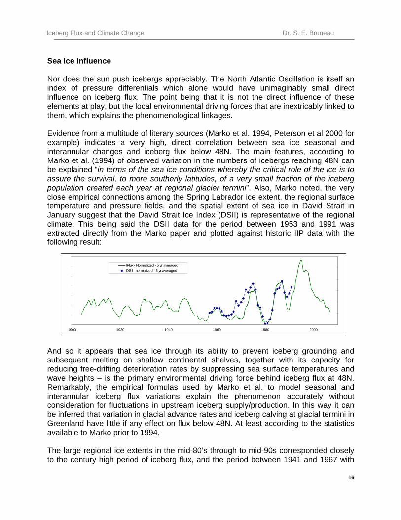
Sea Ice Influence Nor does the sun push icebergs appreciably. The North Atlantic Oscillation is itself an index of pressure differentials which alone would have unimaginably small direct influence on iceberg flux. The point being that it is not the direct influence of these elements at play, but the local environmental driving forces that are inextricably linked to them, which explains the phenomenological linkages. Evidence from a multitude of literary sources (Marko et al. 1994, Peterson et al 2000 for example) indicates a very high, direct correlation between sea ice seasonal and interannular changes and iceberg flux below 48N. The main features, according to Marko et al. (1994) of observed variation in the numbers of icebergs reaching 48N can be explained “in terms of the sea ice conditions whereby the critical role of the ice is to assure the survival, to more southerly latitudes, of a very small fraction of the iceberg population created each year at regional glacier termini”. Also, Marko noted, the very close empirical connections among the Spring Labrador ice extent, the regional surface temperature and pressure fields, and the spatial extent of sea ice in David Strait in January suggest that the David Strait Ice Index (DSII) is representative of the regional climate. This being said the DSII data for the period between 1953 and 1991 was extracted directly from the Marko paper and plotted against historic IIP data with the following result: And so it appears that sea ice through its ability to prevent iceberg grounding and subsequent melting on shallow continental shelves, together with its capacity for reducing free-drifting deterioration rates by suppressing sea surface temperatures and wave heights – is the primary environmental driving force behind iceberg flux at 48N. Remarkably, the empirical formulas used by Marko et al. to model seasonal and interannular iceberg flux variations explain the phenomenon accurately without consideration for fluctuations in upstream iceberg supply/production. In this way it can be inferred that variation in glacial advance rates and iceberg calving at glacial termini in Greenland have little if any effect on flux below 48N. At least according to the statistics available to Marko prior to 1994. The large regional ice extents in the mid-80’s through to mid-90s corresponded closely to the century high period of iceberg flux, and the period between 1941 and 1967 with

0

0.5

1

1.5

2

2.5

3

3.5

1900 1920 1940 1960 1980 20000.6

0.8

1

1.2

1.4

1.6

1.8

IFlux - Normalized - 5 yr averagedDSII - normalized - 5 yr averaged

17


significantly lower ice extents clearly corresponded to the significantly lower numbers of icebergs in that timeframe. Sea temperatures were inversely proportional to ice extent as expected; however, the relationship of sea ice coverage represented by DSII to global mean temperatures was the opposite. Available data suggests that for the period between 1950 and 1990 the affect of Global Mean temperature changes was to have an opposing influence on Labrador Sea surface temperatures and sea ice extents. It is quite uncertain whether this coupling continues to be the case as there have been historic lows in Baffin Bay ice indices in recent times while global temperatures appear to have climbed. The time scale of these recent events (within the past decade) may be too short to determine whether solar activity is responsible, or whether an anomalous and/or anthropomorphic global greenhouse effect is at work. In any case, the conclusion is the same – sea ice severity is the primary control agent for iceberg flux, and the sun is implicated as the primary controlling agent of sea ice. Apparent Modal Behaviour The last comment on this investigation of iceberg climate is on a curious result noticed while plotting histograms of the number of years in which certain numbers of icebergs were observed. Below, the IIP flux data has plotted four times with bin size being the only dependant variable:

Iceberg Frequency 1900-2007 from IIP

0

2

4

6

8

10

12

14

16

18

0

100

200

300

400

500

600

700

800

900

1000

1100

1200

1300

1400

1500

1600

1700

1800

1900

2000

2100

2200

2300

Annual Iceberg Flux across 48N

Yrs

of O

ccur

renc

e

0

5

10

15

20

25

30

35

0

200

400

600

800

1000

1200

1400

1600

1800

2000

2200

18


By plotting in this way iceberg flux rate at 48N gives the subtle impression that it occurs naturally in multiples of around 450. With the exception of the many years in which fewer than 100 bergs were sighted – the modes of the distribution show highest annual frequencies for 400, 900, 1400 and 1800 bergs respectively, with the furthest outlier at 2300. This trend is more apparent in the first two histograms and is not present in the fourth. Whether this is a real, statistically relevant result or the artifact of plotting coincidence and bin size selection is certainly debatable. It would be interesting to speculate on the cause of such a thing if it were indeed proven to be real. The author plans to do follow on work on this subject.


05

101520253035404550

200 400 600 800 1000 1200 1400 1600 1800 2000 2200 2400

Annual Iceberg Flux across 48N


0

10

20

30

40

50

60

70

400 800 1200 1600 2000 2400Annual Iceberg Flux across 48N

19


ICEBERG MODELING STRATEGIES FOR CLIMATE CHANGE Previous sections of this report describe

- the installation and checking of the localberg model, - an extension of sensitivity runs aimed at isolating the most important

environmental driving force parameters, - an experiment involving ranges of inputs and subsequent ANOVA work to see if

parameters are processed within the code in a way that approximates the physics intended,

- and then an overview of the iceberg climate and driving forces that should be considered when investigating long term shifts in met-ocean conditions.

Reflecting on the results of this work leads one to ask the following questions:

1. Is the CIS model code preferred for advancing climate study work in light of the inter-annular characteristics identified earlier in the study?

2. What should be done here to facilitate the mandate of this project? 3. Are there improvements or changes to the physics in the model that should be

made at this point if new code approaches are to be undertaken? (1) The use of the localberg model for experimenting with hypothetical, representative iceberg events has been demonstrated. The tool provides deterministic results for support of hypotheses that may be conjectured and in that way is fully capable. Beyond discrete event modeling, however, lays the realm of simulation for which the localberg code is not preferred. It is the judgment of this Author that for advanced work on Iceberg Flux and Climate Change the preferred programming structure would have different characteristics, more in line with those in the table below:

Desired Attributes of Simulation Programming

environment object oriented, encapsulated, methodolgies with inheritance

program platform matlab or other

data entrydeterministic or probabilistic, manual or automated, simulated or real time

data output user defined according to input

result text and/or plot and/or graphical

integration environmentcommon to international data - class and object oriented structure

simulation procedure integrated into program environment

20


The outcome of using this coding approach would be to enable:

- unlimited numbers of simulated iceberg seasons with user-modified statistics of the input parameters thus enabling long term analyses

- Through a matrix based platform, the easy meshing of distributed environmental data free for users to access from archives or in real time over the internet

- The use of this data resource to mine historic states and thus calibrate model physics using hind casting techniques, and,

- the use of real time data for automated and continuous functioning with built-in feedback calibration capabilities.

An example of the type of resource available for data mining and integration is the North American Regional Reanalysis (NARR) environmental data resource. The NOMADS framework that NARR uses is, “… a distributed data system that promotes the combining of data sets between distant participants using open and common server software and methodologies. Users effectively access model and observational data and products in a flexible and efficient manner from archives or in real-time through existing Internet infrastructure.” The met-ocean data for the region of interest in this study is, apparently, updated every 3 hours, and is thus, not truly real-time. (2) Though somewhat beyond the mandate of this work, but as a direct result of the lessons learned within it, iceberg drift and deterioration physics as used by the Canadian Ice Services have been programmed in Matlab. It is the intention of the author to use this code to pursue advanced iceberg simulations outside the scope of this project but for the benefit of the CIS over the longer term. A Matlab approach was used owing to its flexible user interface which allows the model to be manipulated easily and for graphical representation of results. A student researcher Evan Martin, provided technical support with this work and must be credited with translating many conceptual plans into functioning results. Within the object oriented programming approach Environment and Iceberg classes have been defined so that a large number of inputs can be handled easily and the defaults can be identified for missing inputs. Both drift and deterioration models are implemented as a single Method – of the Iceberg class. The Forecast Method solves the coupled ordinary differential equations which govern the two Methods, using built-in ODE solvers. The Forecast Method has the ability to simulate quasi-dynamic environments by using multiple environmental inputs and dividing the total forecast time into sub-steps, each with a unique environment. At this point the use of Environmental objects only allows for environments that are static in both time and location. This is fine for the bathymetry and land masking which have now been incorporated. However, other dynamic environments require attention - a method for correcting this problem is proposed in which maps of environmental properties are used as inputs instead of discrete values. Data from the NARR described above are the intended target of this exercise. This action allows for the full spatial extent of the region to be modeled, while the temporal changes between reloading of

21


data maps would still have to be resolved by using time-intervals. The use of real-time, or at least frequently updated, data maps would solve one of the key issues – that of interdependency or parametric correlation. Presently it is not known whether qualifiers within the localberg code prevent correlated parameters from diverging or varying in unrealistic and improbable ways. (3) The following questions, being somewhat rhetorical in nature are intended to subjectively comment or raise attention to certain aspects of the model physics as requested in communication with the client, CIS. Though provocative for those on the receiving end, they are intended to lead to constructive results and dialog:

Where so few environmental driving parameters are relevant to the combined drift and deterioration model output is it not prudent to consider replacing the discretized approach with a simple consolidated empirical equation? And further, is it dangerous to separate the various categories of deterioration through a subset of formulas, and likewise do the same with drift – where in fact nature does not apply its driving forces in this way? The state of an iceberg and the state of the environment as described by wind, waves, current and temperature are intertwined in a complex correlated continuum which may best be described in a probabilistic framework – rather than a discrete theoretical one. Are statistical approaches like multivariable regression formulation or learned behavior through neural networks a more pragmatic approach to this dilemma? Given that sea ice plays such a dominant role why is there no direct accommodation of it? And are the environmental driving parameters that are used to infer the effects of ice, sufficient or should the model view these things in reverse, with sea ice being the primary input? The low latitude mandate of the CIS does not sufficiently explain the absence of ice in the model as ice is clearly dominant when it is present, ice coverage and type are perhaps the most readily available data on hand for the CIS, and it is nowhere obvious that localberg is described as being limited in its range of applicability. Are ‘forced’ and ‘buoyant’ convection phenomena mutually exclusive and should the formulas be linked? Are the uncertainties with these approaches so high as to render the formulations entirely empirical in nature, and thus inextricably coupled? In the absence of any capability or accommodation of solar insolation as it relates to weather, is it reasonable to suggest that it is represented in this model? By extension, where parameters are incorporated into the model but are shown to be of negligible value to the variance of output should they remain as stated, or should they be consolidated into dimensionless empirical coefficients, constants or approaches? Is it of value to have parameters included by name, and not by real affect, or is this potentially hazardous to model evolution and improvement? What other fields of science require this sort of programming and forecasting and how is it achieved? Are the iceberg drift models now used in the Barents Sea by Russian researchers of any value or applicability in this area? How much field data is required to achieve desired levels of confidence in modeling and how may it best be gathered?

22


ICEBERG DETERIORATION FIELD WORK - JUNE 2007, ST.JOHN’S This section of the report describes previously unreported results of fieldwork involving the monitoring of a grounded iceberg near Signal Hill in St. John’s, NL in June 2007. The analysis reported here is limited to calving frequency as it relates to previous work by this author through collaboration with Ballicater (1998, 2004, and 2005) On the morning of June 3rd 2007 an iceberg was observed in the distance from Signal Hill St. John’s as it drifted a general course to the South West. There were approximately two other bergs within sight at that time. Fortuitously, the author photographed this distant iceberg and returned the next day to find that it had drifted in to shore and apparently grounded in the general vicinity referred to as Quidi Vidi. The berg was again photographed in the same area the following day and the author then contacted the CIS with a request for the expeditious return of camera equipment used in prior time-lapse field work. Continued daily trips to the lookout confirmed that the berg was indeed grounded and likely to stay as it had drifted into place as a tabular one. These, is has been observed will remain in place through a considerable period of deterioration owing to the fact that in tabular form a minimum draught is achieved and subsequent melting which may cause imbalances usually serve to increase the downward reach of one side or another of the ice mass. On June 9th the equipment arrived from the CIS and through a prior agreement with National Parks Historic sites two independent recording stations (laptop, tripod, video camera . . .) were configured and launched from within the Marconi room in Cabot Tower. Approximately Parallel camera records for 9 complete days were managed through twice-daily visits to the Tower. As usual, fog, darkness and iceberg repositioning out sight meant that a cumulative total of only 72.25 hours of unambiguous eligible records were obtained. In all instances the better of the two views from the camera setups was selected for any particular recording interval. (The strategy with two cameras being a near field view with good resolution and high risk of iceberg departure from the viewfinder, and, a wide angle with poorer resolution but a fighting chance of keeping the berg within sight during unmanned periods.) In a manner similar to that described in some detail in previous work (Ballicater 2004, 2005) the time lapse data were reduced and scrutinized for calving events. The observed events have been categorized as small, medium and large according to the following classification: Small - Single growler, few bits of brash. Medium - A few large pieces, several smaller and a noticeable halo of brash in the

surrounding water. Large - Noticeable change in berg shape and orientation, large quantities of

floating ice rubble of all sizes, some sintered piles of brash noticeable.

23


Summary of Calving Events at Signal Hill The table below lists the events noted from the record:

Calving Events Date/Time Size

6/09/10:04 Small 6/11/14:36 Small 6/09/13:55 Small 6/11/16:31 Large 6/09/15:22 Small 6/11/17:07 Small 6/09/16:23 Medium 6/12/9:01 Medium 6/09/17:01 Small 6/12/10:38 Small 6/09/21:28 Small 6/12/11:31 Medium 6/10/10:21 Small 6/12/12:58 Small 6/10/11:06 Medium 6/15/9:34 Small 6/10/17:11 Large 6/15/11:42 Large 6/10/18:13 Small 6/16/8:00 Medium 6/11/4:41 Small 6/16/11:30 Large 6/11/7:45 Small

These results have been graphically represented below on a timeline whereby periods of valid data are differentiated from lost time. Fisheries and Oceans Canada records bi-monthly sea surface temperatures in the oceans surrounding the country. The temperatures are recorded by satellite over a period of half a month and are then averaged and placed in a composite is shown in the figure below. The composite for June 1 – 15th showed an average temperature of 7oC, and the composite for June 15 – 30th displayed an average temperature of 10oC. Given the observation period extended from June 9th to June 17th it has been assumed that an average temperature of 8oC was experienced during the observation period.

June 9 June 10 June 11 June 12 June 13 June 14 June 15 June 16 June 17

GREEN Periods of clear viewGREY DarknessBLUE FogYELLOW Out of view

June 9 June 10 June 11 June 12 June 13 June 14 June 15 June 16 June 17June 9 June 10 June 11 June 12 June 13 June 14 June 15 June 16 June 17

GREEN Periods of clear viewGREY DarknessBLUE FogYELLOW Out of view

24


The Marine Environmental Data Service of DFO provides hydrographic information for many sites, and significantly this includes data from a station not four kilometers from the berg grounding site. On June 15th, 2007 at 47.55oN and 52.59oW a STD profile was obtained in the vicinity shown on the figure below:

25


The STD profile plotted below indicates a near surface temperature between 5 and 6 degrees C though the resolution at this depth is vague, and it appears readings above 5 meters are non-existent. Regardless, extrapolation suggests the NOAA data for SST is a match and for future work the STD profile over depth may be of importance for re-analyzing this deterioration event. Analysis and Discussion During the 72.25 hours of observation time 14 small, 5 medium and 4 large events were recorded. The average calving interval during this time period for both medium and large events combined was 8.0 hours. The plot below indicates the relative goodness of fit of the present data with past work. The round markers on the graph represent the calving intervals for medium and large events. Only the medium and large events were used because it is unlikely that the smaller events were able to be seen during the observations from the air. Upper and lower limits have been added to the 2007 data to represent the range of the actual calving rate. The upper limit is developed by recording the large calving events. During the 2007 observations there were 4 large events leading to a calving interval of 18.1 hours. The lower limit is developed by recording all (small, medium and large) calving events, this leads to a calving interval of 3.1 hours. The upper and lower limits have been displayed on Figure 3 for the 1998, 2000 and 2004 data points as well. Of note: previous investigations resulting in calving interval data have been undertaken from both air and on land. The calving intervals from 2000 to 2003 were obtained from CFR flights and the data in 1998 and 2004 were obtained from video observations much like the present 2007 data.

26


The straight dashed line on the graph represents the best linear fit through all data points. The equation of the line is given by:

tc = 49.2 – 4.66Tw Where tc is the calving interval in hours and Tw is the surface water temperature. Reasonable agreement results from the linear model (R2 = 0.8084) but it poses problems reconciling with natural tendencies towards the extremes. To avoid a calving interval tending towards zero as temperatures rise past 10oC, and, appreciable calving rates in waters well below zero, a declining exponential best fit was applied with the resulting curve formulation:

tc = 59.4 * e(- 0.205Tw

)

Whether this fit is better or not within the context of CIS iceberg modeling is unknown. By comparison, in Ballicater (2004) similarly derived empirical formulas from the 4 CFR data points were expressed as:

tc = 55.3 – 5.3Tw tc = 62 * e(- 0.20Tw

)

Note that subtle changes in coefficients and exponents have resulted from the addition of new data to the analysis.

1998

2000

2001

2002

2003

20042007

0

10

20

30

40

50

60

-2 0 2 4 6 8 10 12 14

Sea Surface Temperature (oC)

Cal

ving

Inte

rval

(hou

rs

Documents

Report Iceberg Flux and Climate Changesbruneau/research/publications/2008cis.pdf · Report Iceberg Flux and Climate Change FOR THE CANADIAN ICE SERVICE JUNE 2007 - MARCH 2008 Submitted