On climate response to changes in the cosmic ray flux and

On climate response to changes in the cosmic ray

flux and radiative budget

Nir J. ShavivRacah Institute of Physics, Hebrew University of Jerusalem, Jerusalem, Israel

Received 27 October 2004; revised 11 May 2005; accepted 1 June 2005; published 23 August 2005.

[1] We examine the results linking cosmic ray flux (CRF) variations to global climatechange. We then proceed to study various periods over which there are estimates forthe radiative forcing, temperature change and CRF variations relative to today. Theseinclude the Phanerozoic as a whole, the Cretaceous, the Eocene, the Last GlacialMaximum, the 20th century, as well as the 11-yr solar cycle. This enables us to placequantitative limits on climate sensitivity to both changes in the CRF, and the radiativebudget, F, under equilibrium. Under the assumption that the CRF is indeed aclimate driver, the sensitivity to variations in the globally averaged relative change in thetropospheric ionization I is consistently fitted with m � � (dTglobal/dI) � 7.5 ± 2�K.Additionally, the sensitivity to radiative forcing changes is l � dTglobal/dF = 0.35 ±0.09�KW�1m2, at the current temperature, while its temperature derivative is undetectablewith (dl/dT)0 = �0.01 ± 0.04 m2W�1. If the observed CRF/climate link is ignored,the best sensitivity obtained is l = 0.54 ± 0.12�KW�1m2 and (dl/dT)0 = �0.02 ±0.05 m2W�1. Note that this analysis assumes that different climate conditions can bedescribed with at most a linear function of T; however, the exact sensitivity probablydepends on various additional factors. Moreover, l was mostly obtained throughcomparison of climate states notably different from each other, and thus only describes anaverage sensitivity. Subject to the above caveats and those described in the text, theCRF/climate link therefore implies that the increased solar luminosity and reducedCRF over the previous century should have contributed a warming of 0.47 ± 0.19�K, whilethe rest should be mainly attributed to anthropogenic causes. Without any effect of cosmicrays, the increase in solar luminosity would correspond to an increased temperature of0.16 ± 0.04�K.Citation: Shaviv, N. J. (2005), On climate response to changes in the cosmic ray flux and radiative budget, J. Geophys. Res., 110,

A08105, doi:10.1029/2004JA010866.

1. Introduction

[2] Accumulating evidence suggests that solar activity isresponsible for at least some climatic variability. Theseinclude correlations between solar activity and either directclimatic variables or indirect climate proxies over timescales ranging from days to millennia [Herschel, 1796;Eddy, 1976; Labitzke and van Loon, 1992; Friis-Christensenand Lanssen, 1991; Soon et al., 1996a, 2000; Beer et al.,2000; Hodell et al., 2001; Neff et al., 2001]. It is thereforedifficult at this point to argue against the existence of anycausal link between solar activity and climate on Earth.However, the climatic variability attributable to solar activ-ity is larger than could be expected from the typical 0.1%changes in the solar irradiance observed over the decadal tocentennial time scale [Beer et al. 2000; Soon et al., 2000].Thus, an amplifier is required unless the sensitivity tochanges in the radiative forcing is uncomfortably high.

[3] The first suggestion for an amplifier of solar activitywas suggested by Ney, who pointed out that if climate issensitive to the amount of tropospheric ionization, it wouldalso be sensitive to solar activity since the solar windmodulates the cosmic ray flux (CRF), and with it, theamount of tropospheric ionization [Ney, 1959].[4] Over the solar cycle, the interplanetary magnetic field

varies considerably, such that the amount of troposphericionization changes by typically 5%. Svensmark [1998,2000], Marsh and Svensmark [2000a] as well as Palle Bagoand Butler [2000] have shown that the variations in theamount of low altitude cloud cover (LACC) nicely correlatewith the CRF reaching Earth over two decades. A recentanalysis has shown that the latitudinal variations of theLACC are proportional to the latitudinal dependence of thelow altitude ion concentrations [Usoskin et al., 2004a]. Thissuggests that it is more likely that the cloud cover is directlyrelated to the CRF than directly to solar activity.[5] More recent data on the LACC seems to exhibit a

weaker correlation with the variable CRF [e.g., Farrar,2000]. There are however a few peculiarities in the data

JOURNAL OF GEOPHYSICAL RESEARCH, VOL. 110, A08105, doi:10.1029/2004JA010866, 2005

Copyright 2005 by the American Geophysical Union.0148-0227/05/2004JA010866$09.00

A08105 1 of 15

which are indicative of a calibration problem, which onceremoved, seem to recover the high correlation between theCRF and the LACC [Marsh and Svensmark, 2003]. For anobjective review, the reader is encouraged to read Carslawet al. [2002].[6] The above correlations between CRF variability and

climate (and in particular, cloud cover), indicate that CRFmodulations appear to be responsible for climate variability,most probably through modulation of the amount of LACC.Nevertheless, since all of the above CRF variability ulti-mately originates from solar activity changes, it is notpossible to unequivocally rule out the possibility that theCRF/climate correlations are coincidental, and that both areindependently modulated by solar activity with similar lags.[7] An independent CRF/climate correlation on a much

longer time scale, in which variations in the CRF do notoriginate from solar variability, was found by Shaviv[2002a, 2002b] and Shaviv and Veizer [2003]. It was shownusing astronomical data that the CRF should change bymore than a factor of 2 because of our passages through thegalactic spiral arms, with a period of 132 ± 25 Ma [Shaviv,2002b]. It was also shown that the CRF history can actuallybe reconstructed using the cosmic-ray exposure age data ofIron meteorites, exhibiting a periodicity of 143 ± 10 Ma anda phase consistent with the astronomical data. Moreover, itwas found that the reconstructed CRF nicely synchronizesto the occurrence of ice-age epochs on Earth, whichappeared on average every 145 ± 7 Ma over the past billionyears. Additionally, the mid-point of the ice-age epochs ispredicted to lag by 31 ± 8 Ma after the mid-point of thespiral arm crossing, while it is observed to lag by 33 ±20 Ma. That is, the CRF and ice-age epoch signals agree inboth phase and period. The same analysis also revealed thatthe long term star-formation activity of the Milky Waycorrelates with long term glacial activity on Earth. Inparticular, a dearth in star formation between 1 and 2 Gabefore present, coincides with a long period during whichglaciations appear to have been totally absent [Shaviv,2002b, 2003].[8] We should also point out several experimental results

supporting, though not proving yet, a CRF/cloud coverlink. Harrison and Aplin [2001] found experimentally thatCN formation is correlated with natural Poisson variabilityin cosmic ray showers. In other words, this link appears tobe more than hypothetical. In another set of experiments, itwas shown that cosmic rays play a decisive role in theformation of small clusters [Eichkorn et al., 2002]. If thesesmall clusters can be shown to grow quickly enough, asopposed to being scavenged by large particles, the linkbetween cosmic rays and the formation of cloud conden-sation nuclei and ultimately cloud cover could be firmlyestablished.[9] We will not dwell here on the actual mechanism

responsible for CRF link with cloud behavior. We willsimply assume henceforth that this link exists, as supportedby empirical and experimental data, even though it is still anissue of debate. This point has to be kept in mind since theconclusions we shall reach, will only be valid if thisassumption is correct.[10] Using the above assumption, we study several time

scales to see whether estimates on global temperaturesensitivity can be placed, together with estimates on the

CRF/temperature relation. We will do so by comparing theobserved temperature changes with changes in the radiativebudget, an approach previously pursued in numerousanalyses [e.g., Hoffert and Covey, 1992; Covey et al.,1996; Hansen et al., 1993; Gregory et al., 2002]. Thismethod for obtaining the global temperature sensitivityusing paleodata is orthogonal to the usage of globalcirculation models (GCMs) upon which often quotedresults are based [IPCC 2001]. Hence, the two methodssuffer from altogether different errors. It is therefore clearlyadvantageous to follow this path as an independent esti-mate. For example, Cess et al. [1989] have shown that thelarge uncertainty in the sensitivity obtained in GCMs stemsfrom the uncertain feedback of cloud cover. Since we usethe actual global data, all the feedbacks are implicitlyconsidered. The main contribution in this work is tospecifically consider the contribution of the CRF to thechanged radiative budget. As a note of caution, one shouldkeep in mind that the most notable assumption in thismethod is the quantification of climate sensitivity with onenumber. In other words, it assumes that on average Earth’sclimate responds the same irrespective of the geographic,temporal or frequency space distribution of the radiationbudget changes. It also assumes that different radiativeforcings act linearly.[11] Once the radiative forcing and temperature changes

are obtained, the sensitivities can be estimated with

l � dTglobal

dF

��F¼F0

� DT

DF: ð1Þ

DF, which is the globally averaged change in the radiationflux (per unit surface area), will also include here thecontribution DFCRF arising from a changed energy flux f ofcosmic rays. Note also that over short time scales, DT or DFhave to be properly modified to include the finite heatcapacity of the system, and the consequent finite adjustmenttime it has. We should also consider the possibility that l isdependent on the temperature. For example, the positiveclimate feedback arising from the formation of ice sheetscould increase the sensitivity of a glaciated Earth, while thereduced atmospheric water vapor content, can reduce thesensitivity.[12] In addition to l, we will also estimate the sensitivity

to CRF variations, or more specifically, to changes in theglobal atmospheric ion density.

2. Radiative Forcing of Low AltitudeCloud Cover

[13] Without a detailed physical model for the effects ofcosmic rays on clouds or a detailed enough record ofradiation budget measurements correlated with the solarcycle, it is hard to accurately determine the quantitative linkbetween CRF variations and changes in the global radiationbudget. In particular, it is hard to do so without limitingourselves to various approximations. Nevertheless, this linkis important since it will be used in most of our estimates forthe global temperature sensitivity.[14] The basic observation we use to estimate the radia-

tive forcing of clouds is the apparent correlation betweenCRF variations and the amount of low altitude cloud cover.

A08105 SHAVIV: COSMIC RAYS AND CLIMATE SENSITIVITY

2 of 15

A08105

A naive approximation is to assume that the whole climaticeffect can be described by variations in the extent of thecloud cover, namely, that we neglect effects in the cloudproperties, or possible climatic effects associated withatmospheric ionization but not with clouds. It also impliesthat the geographical distribution of the effect is the same aslow altitude clouds on average. We will first estimate this‘‘zeroth’’ order term and then try to estimate the possiblecontribution of other corrections.[15] Amount of cloud cover: Over the solar cycle, the

varying CRF appears to cause a 1.2 to 2.0% (absolute)change in the amount of LACC [Marsh and Svensmark,2000b; Kirkby and Laaksonen, 2000; Marsden andLingenfelter, 2003; Carslaw et al., 2002]. We will thereforeadopt a change of 1.6 ± 0.4% in the LACC.[16] The total radiative forcing of the LACC is estimated

to be �16.7 Wm�2 from the average 26.6% cloud cover[Hartmann et al., 1992]. If one however compares theforcing of the total cloud cover from different hemispheresand different experiments (Nimbus and ERBE [Ardanuyet al., 1991]), one finds variations which are typically2.5 Wm�2 on the �50 Wm�2 shortwave (SW) ‘‘cooling’’and 7 Wm�2 on the 27 Wm�2 longwave (LW) ‘‘warming’’.Since LACC typically comprise half of the total amountcloud cover, an error of �4 Wm�2 is to be expected.[17] Thus, the changed radiative forcing DFf associated

with the varying amount of cloud cover, should be �1.0 ±0.35 Wm�2. This implicitly assumes that the incrementalcloud cover has the same average net radiative properties asthe whole 27% of the LACC.[18] Cloud optical depth: Changes in the cloud properties

could take place in addition to changes in the cloud amount.According to Marsden and Lingenfelter [2003], there is asmall negative correlation between the average LACCopacity �t and the varying CRF. Over the solar cycle, �tchanges by �4% relative to its global average of about 4 inregions defined to be covered by LACC.[19] Is such a change in �t reasonable? According to

Marsden and Lingenfelter [2003], there are two limitingcases for the effects on cloud properties. The first ischanging the number density of cloud condensation nuclei(CCN) given a fixed amount of Liquid Water Content(LWC), that is, CCN limited. This is similar to the‘‘Twomey effect’’ where enhanced aerosol density affectsthe droplet size and cloud albedo [Twomey, 1977;Rosenfeld, 2000]. The second case is increasing the CCNdensity together with the LWC, and obtaining similar sizeddrops (LWC limited). Although the two cases are plausible,they do not change the cloud properties in the same way.[20] One can show that a cloud’s optical depth for SW

absorption is [e.g., Marsden and Lingenfelter, 2003]

t � 3

2

reffDzr0Reff

; ð2Þ

where r0 is the density of water, reff is the mass loading ofwater (i.e., its effective density), Dz is the vertical extentof the cloud and Reff is the effective radius of thecloud droplets, defined as the ratio between the 3rd and2nd moments of the droplet distribution (hr3i/hr2i). Inthe case of a CCN limited condensation, Reff / nCCN

�1/3, and

t will increase with nCCN, while in the LWC limiting case,

reff / nCCN and t will increase as well. One can thereforewrite:

dtt¼ b

dnCCNnCCN

; ð3Þ

with b = 1 for LWC limited case and b = 1/3 for the CCNlimited case. Since the lower troposphere ionization ratechanges by about 7% between solar minimum andmaximum, we should expect to get at most a similarincrease in the CCN. Thus we should expect dt/t ] 7%.The fact that a negative change in t was observed [Marsdenand Lingenfelter, 2003], could arise because the increase incloud lifetime results with thinner clouds on average.[21] Next, one can approximate the relation between t

and cloud albedo A, by the relation [Hobbs, 1993]:

A � ttþ t1=2

; ð4Þ

where t1/2 � 6.7 for an asymmetry parameter of 0.85[Hobbs, 1993]. Once we differentiate, we find:

dAdt

�A2t1=2t2

: ð5Þ

If we consider the transmission T � 0.75 of the atmosphere(to obtain a top-of-atmosphere albedo, from a cloud-topalbedo), that the LACC covers only a fraction flow of theglobe, and that the average top-of-atmosphere incidence ofradiation is �F = 344 Wm�2, we find that the change inalbedo is responsible for a changed radiation budget of

DFA �A2t1=2t2

�FT 2flowd�t � þ0:13Wm�2: ð6Þ

The positive sign implies that the small apparent reductionin �t contributes a small warming contribution.[22] If we had no knowledge of �t, changes in it could

have resulted with a correction to DFA which are only aslarge as�0.23 Wm�2 (for the LWC limited case, and dt/t]7%). We take this uncertainly in �t as another source of errorfor the radiative forcing DF.[23] Cloud emissivity: There could still be more physical

terms contributing to DF. If the LWC in the clouds can varyas well (that is, the clouds are not CCN limited but ratherwater limited), then also the IR emissivity can change. Itwill do so by changing the emissivity, relative to black body[e.g., Stephens, 1978] which is given by

� Dzð Þ ¼ 1� exp �tIRð Þ: ð7Þ

where we have defined tIR � a0reffDz. Here, reff is theliquid water content, a0 is the mass absorption coefficient(for water clouds, a0 � 0.13 m2g�1 [Stephens, 1978]) and dzis the thickness of the cloud layer above a given point. Bychanging the emissivity, we change the outgoing long-wavelength flux by

DFIR ¼ T sT4flowD� ¼ exp �tIRð ÞT sT4tIRDreffreff

ð8Þ


3 of 15

A08105

where T � 0.6 is the transmittance of the atmosphere to IR,above the cloud. For typically small values of reff of 0.3 g/m

3,and dz = 100 m (which would give the largest effect), weget corrections of DFIR = 1.1Wm�2 (Dreff/reff)] 0.1 Wm�2.This positive flux outwards tends to cool (i.e., increase theCRF/temperature effect), but it is a small effect.[24] By changing the emissivity, we can also shift the

apparent location of the top of the clouds, and with it theirtemperature. In other words, we should expect outgoing LWradiation to come from higher up the atmosphere where thetemperature is lower.[25] A higher reff will shift the IR emission ‘‘surface’’

vertically by typically:

Dz � 1

a0reff

Dreffreff

� �: ð9Þ

Using the black body law, the change in the radiativeemission over the solar cycle will therefore be less than

�DFDT<� flow4sT3DzdT

dz<� 0:2

Dreffreff

Wm�2; ð10Þ

once globally averaged. For the last inequality, we took atypically low reff of 0.3 g/m3, a wet adiabat of dT/dz �0.6�K (100 m)�1 and flow � 0.28. Since Dreff/reff ] 0.1, thiseffect will be even smaller at best (and in opposite sign asthe previous effect).[26] This result is also reasonable considering that the

total long wavelength heating effect of LACC was estimatedto be �3.5 Wm�2 [Hartmann et al., 1992], while cloudalbedo is responsible for a globally averaged cooling of�20 Wm�2, implying that changes in albedo will likely bemore important for changing the radiative budget arisingfrom LACC variations.[27] Ocean bias: Additional unaccounted effects are pos-

sible. For example, we implicitly assumed before that theeffects of a changed LACC on the radiation budget can bedescribed by the average effect of LACC. This would be thecase if the geographic distribution of the LACC variations isthe same as the distribution of the average LACC. This neednot be the case. Specifically, we expect the CRF effect to bemore dominant in marine environments, where CCN arerelatively scarce. But the average radiative properties ofLACC over oceans is different than the globally averagedproperties of LACC. This is because covering or uncoveringthe ocean with clouds corresponds to a different change inthe albedo than those arising from covering or uncoveringland.[28] Quantitatively, the Earth’s albedo can be approxi-

mated with

A ¼ al flAc þ 1� flð ÞAl½ � þ ao foAc þ 1� foð ÞAo½ � ð11Þ

where al � 1/3 and ao � 2/3 are the surface fractionscovered by land and oceans, respectively. Ac is the averagecloud albedo, Al and Ao are the average cloudless land andocean albedos, while fl and fo are respectively the fractionsof land and ocean covered with clouds.[29] An unbiased LACC/CRF effect would change the

total cloud cover while keeping fixed the ratio r� fl/fo� 0.5.

If on the other hand all the LACC variations associatedwith a changed CRF are limited to the oceans, then fl iskept fixed. The additional albedo change associatedwith the biased case, as compared with the unbiased casecan be straightforwardly calculated to be DA � (Al �Ao)r (1 � ao)/(r + ao � rao) Dflow � 0.03 Dflow, wherewe have assumed Al � Ao � 15%. This corresponds to aflux change of DFDA � DAT 2 �F � +0.1 Wm�2 over thesolar cycle. That is, a likely ocean bias implies that we areslightly underestimating DFCRF.[30] Other effects: If the effect is geographically localized

to certain areas, then a larger discrepancy could arise if theradiative properties of the LACC over those geographicregions is significantly different from the properties ofLACC on average. A correlation map between LACCvariations and CRF change [Marsh and Svensmark,2000b], reveals that some regions (particularly over oceans)stand out with a higher correlation than others. Neverthe-less, they do not appear to cluster around particular latitudesor other special regions. Thus, the assumption of geographicuniformity may be not that bad.[31] Another hard to estimate effect could arise from the

expected increase in cloud lifetime. For example, cumulus-type clouds could penetrate into higher altitudes, therebyreducing their IR emission.[32] Thus, until we fully understand all the details in the

physical picture, we should take the estimated radiativeforcing and the error with a grain of salt. Taking the aboveinto considerations, our best estimate for the radiativeforcing of the cloud cover variations over the solar cycleis DFCRF = DFf + DFA + DFDA = 1.0 ± 0.4Wm�2, globallyaveraged (we have neglected DFIR ] 0.1 Wm�2 and�DFDT ] 0.02 Wm�2). This should be compared with the0.1% solar flux variations, giving rise to an extra ‘‘direct’’forcing of DFflux � 0.35 Wm�2 [Frohlich and Lean, 1998].[33] Our goal here, is to find a number describing the

relation between CRF variations and changes in the radia-tive forcing. However, instead of working with the CRFitself, we will work with I , the cosmic ray inducedionization (CRII), which is the global average of the relativechange in the atmospheric ion density. We do so, because, itwas found empirically that the LACC change is linear inthis value [Usoskin et al., 2004a]. This relation appears tohold even locally at given latitudinal bands. The CRII itselfis proportional to the square root of the ionization rate, sincethe ion density is dominated by ion-ion recombination[Ermakov et al., 1997].[34] Over the recent solar cycles, the solar modulation

parameter F� has changed between approximately 500 and1000 MeV. Using the results of Appendix A, the CRII haschanged by DI � 4.5%.[35] Thus, we find that the radiative sensitivity to CRF

variations is about

a � � dF

dI ¼ 22� 9Wm�2: ð12Þ

3. Estimating Climate Sensitivity

[36] We now proceed to estimate the climate sensitivity.We do so by comparing the radiative forcing change


4 of 15

A08105

between two eras to the temperature change which ensued,using equation (1). In most estimates, we will rely on theresults of section 2 to obtain the contribution of the changedCRF, and with it changes in the CRII, to the changedradiative forcing. These include seven different compari-sons, spanning from variations over the solar cycles, tovariations over the Phanerozoic as a whole. Subsequently,we will combine the results to obtain our best estimate forthe climate sensitivity.

3.1. DT/CO2 Correlation Over the Phanerozoic

[37] Shaviv and Veizer [2003] have shown that more thantwo thirds of the variance in the reconstructed tropicaltemperature variability DTtrop over the Phanerozoic can beexplained using the variable CRF, which could be recon-structed using Iron meteorites. On the other hand, it wasshown that the reconstructed atmospheric CO2 variations donot appear to have any clear correlation with the recon-structed temperature. The large correlation between recon-structed CRF and temperature is seen in Figure 1. It is thiscorrelation which led the authors to conclude that thePhanerozoic climate is primarily driven by a celestial driver.The lack of any apparent correlation with CO2 was used toplace a limit on the global climate sensitivity. This isbecause changes in the atmospheric CO2 concentrationimply changes to the earth radiative budget.[38] A subsequent analysis by Royer et al. [2004] has

shown that pH corrections could have been important atoffsetting the d18O record upon which the temperature

reconstruction is based. In particular, The pH correctionterm of Royer et al. [2004] has the form:

DTpH ¼ a logRCO2 þ logL tð Þ � logW tð Þf g; ð13Þ

where RCO2 is the atmospheric partial pressure of relative totoday, L(t) is (Ca)(t)/(Ca)(0) - the mean concentration ofdissolved calcium in the water relative to today, while W(t)is [Ca++][CO3

��]/Ksp at time t relative to today. Theexpression for a essentially contains two factors. The firstis a theoretically calculated factor characterizing the effectof pH on d18O. The second is the translation between d18Oand temperature variations. Once the ice-volume effect ond18O is considered [Veizer et al., 2000; Shaviv and Veizer,2004], one obtains: a � 1.4�K.[39] Since the pH correction depends on RCO2, so will the

corrected temperature. A simple correlation between thecorrected temperature and the reconstructed RCO2 will thenbe meaningless. Instead, the method to proceed is to defineda CO2 ‘‘uncorrected’’ temperature as:

DT 0 ¼ DT � a logRCO2: ð14Þ

Any correlation that this signal will have with RCO2 willthen be real, since this ‘‘temperature’’ depends only ond18O, and the small L and W terms. This uncorrectedtemperature can then be fitted with

DT 0model ¼ Aþ Bt þ C � a log10 2ð Þ log2 RCO2 þ Dg f tð Þ½ �: ð15Þ

A and B allow for systematic secular trends in the data.These arise from the well understood solar luminosityincrease and the poorly understood tectonically controlledtrend in the d18O data [Veizer et al., 2000]. D relates thecosmic ray energy flux f(t) to DT [Shaviv and Veizer, 2003].The term (a log102) log2RCO2 was added such that C willkeep its original meaning in Shaviv and Veizer [2003],which is the tropical temperature increase associated with adoubled RCO2.[40] This assumes that the radiative forcing is logarithmic

in RCO2, that is, that DFCO2 � DF�2 log2 [RCO2/(280 ppm)]and that over the entire range of the Phanerozoic, thetemperature sensitivity to DF is constant. Over the orderof magnitude variations in RCO2, the former approximationis good to within 10% of actual calculations [Hansen et al.,1998]. This is good enough considering the uncertainties inthe second approximation, which does appears to be con-sistent with the data (see section 3.8.2). For the effect of adoubled CO2 concentration, we take DF�2 = 3.71 Wm�2

[Myhre et al., 1998]. As for the CO2 reconstruction itself,there are a few to choose from. The analysis describedbelow uses the more common GEOCARB III reconstruction[Berner and Kothavala, 2001], but the limits obtained areactually insensitive to the preferred model [Shaviv andVeizer, 2003].[41] The lack of a correlation between d18O and RCO2

[Shaviv and Veizer, 2003] originates from the fact that (C �alog102) happens to be coincidentally close to 0. In otherwords, the pH correction to d18O and DT happens tobe similar to the tropical temperature sensitivity to changesin RCO2. (Without the pH correction, the preferred value for

Figure 1. The high correlation between the reconstructedtemperature and CRF over the Phanerozoic can be used toestimate global sensitivity. Here, DT0 is the reconstructedtemperature DT of Veizer et al. [2000] binned into 20 Myrbins, over the past 550 Ma, with a small linear temperatureincrease of 1.7�K (t/550 Ma) subtracted [see Shaviv andVeizer, 2003]. The CRF is one of 3 reconstructions used inShaviv and Veizer [2003]. The two others differ in the totalamplitude of variations. The two independent signals have ahigh Pearson correlation of r = �0.70. Although statisticallysignificant limits on p cannot be placed, lower p values arefavored (with p � 0.3 producing the best fit). Nevertheless,the value of p = 0.5 is theoretically preferred. The insetshows the time dependence of the two signals.


5 of 15

A08105

C in the absence of correlation is not a log102, but 0.)Scientifically, this is somewhat unfortunate, because with-out this coincidence the d18O signal would have had a clearcorrelation with the RCO2 signal, and the RCO2 fingerprintwould have been discernible in the Phanerozoic data.[42] If we repeat the analysis of Shaviv and Veizer [2003]

and consider also the effects of a log L(t) � logW(t)introduced by Royer et al. [2004], and corrected for RCO2

as described above, we obtain: C = 0.69�K (or an upperlimit of 1.12, 1.42 and 1.73�K at 68%, 90% and 99%confidence levels, and a lower limit of 0.39, 0.10, �0.21�K,respectively). This gives l = 0.28 ± 0.15�KW�1m2.[43] Without the effect of cosmic rays (i.e., with the D

term removed in the model given by equation (15)), more ofthe reconstructed temperature variability can be explainedwith CO2, and the estimate range for l broadens respec-tively to l = 0.36 ± 0.22�KW�1m2. More limits are given inTable 1.[44] Note that this estimate is independent of a deter-

mined in section 2. The first range for l simply assumes thata CRF/climate link exists, while the second quoted range,even neglects this assumption. Note also that although thereis no reason for the ice-volume effect on the d18O to beabsent, removing it altogether would increase the estimatefor l by � 0.2�KW�1m2,), i.e., just within the error bar.

3.2. CRF/#T Correlation Over the Phanerozoic

[45] The significant correlation between CRF and tem-perature over the Phanerozoic was also used to place limitson the ratio between CRF variations and temperaturechange. Together with the results of section 2 we can placea limit on l.[46] In Shaviv and Veizer [2003], it was found that if

DTtrop is approximated with

DTtrop ¼ D f=f0ð Þp � 1½ �; ð16Þ

where p = 1/2 and f0 is the CRF today, then D = 8 ± 4�K.Using more data to constrain the CRF variations, model (3)of Shaviv and Veizer [2003] with its larger CRF variationscan be ruled out, implying that D should be 5 ± 1.25�K.This can be done once the 10Be-36Cl exposure ages, whichrequire calibration [Lavielle et al., 1999], are considered,since these ages have intrinsically smaller errors andtherefore more clustering, a higher lower limit can beplaced on the CRF variations. Note also that because thegalactic variations in the CRF are mostly energy indepen-dent, the CRF variations in the Iron meteorite data have thesame variations as those of the higher energies responsiblefor the tropospheric ionization. If we generalize to otherpower laws p between 0.25 to 1.5, remember that I / f1/2,

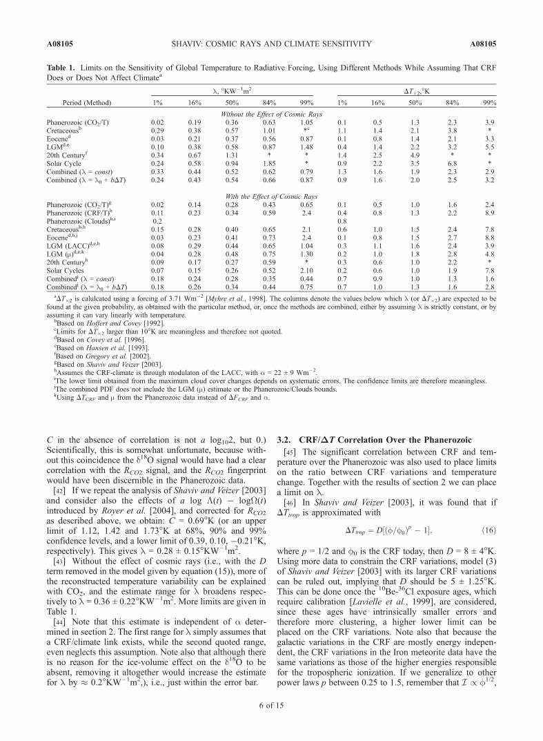
Table 1. Limits on the Sensitivity of Global Temperature to Radiative Forcing, Using Different Methods While Assuming That CRF

Does or Does Not Affect Climatea

Period (Method)

l, �KW�1m2DT�2,�K

1% 16% 50% 84% 99% 1% 16% 50% 84% 99%

Without the Effect of Cosmic RaysPhanerozoic (CO2/T) 0.02 0.19 0.36 0.63 1.05 0.1 0.5 1.3 2.3 3.9Cretaceousb 0.29 0.38 0.57 1.01 *c 1.1 1.4 2.1 3.8 *Eocened 0.03 0.21 0.37 0.56 0.87 0.1 0.8 1.4 2.1 3.3LGMd,e 0.10 0.38 0.58 0.87 1.48 0.4 1.4 2.2 3.2 5.520th Centuryf 0.34 0.67 1.31 * * 1.4 2.5 4.9 * *Solar Cycle 0.24 0.58 0.94 1.85 * 0.9 2.2 3.5 6.8 *Combined (l = const) 0.33 0.44 0.52 0.62 0.79 1.3 1.6 1.9 2.3 2.9Combined (l = l0 + bDT) 0.24 0.43 0.54 0.66 0.87 0.9 1.6 2.0 2.5 3.2

With the Effect of Cosmic RaysPhanerozoic (CO2/T)

g 0.02 0.14 0.28 0.43 0.65 0.1 0.5 1.0 1.6 2.4Phanerozoic (CRF/T)h 0.11 0.23 0.34 0.59 2.4 0.4 0.8 1.3 2.2 8.9Phanerozoic (Clouds)h,i 0.2 0.8Cretaceousb,h 0.15 0.28 0.40 0.65 2.1 0.6 1.0 1.5 2.4 7.8Eocened,h,j 0.03 0.23 0.41 0.73 2.4 0.1 0.8 1.5 2.7 8.8LGM (LACC)d,e,h 0.08 0.29 0.44 0.65 1.04 0.3 1.1 1.6 2.4 3.9LGM (m)d,e,k 0.04 0.28 0.48 0.75 1.30 0.2 1.0 1.8 2.8 4.820th Centuryh 0.09 0.17 0.27 0.59 * 0.3 0.6 1.0 2.2 *Solar Cycles 0.07 0.15 0.26 0.52 2.10 0.2 0.6 1.0 1.9 7.8Combinedj (l = const) 0.18 0.24 0.28 0.35 0.44 0.7 0.9 1.0 1.3 1.6Combinedj (l = l0 + bDT) 0.18 0.26 0.34 0.44 0.75 0.7 1.0 1.3 1.6 2.8

aDT�2 is calulcated using a forcing of 3.71 Wm�2 [Myhre et al., 1998]. The columns denote the values below which l (or DT�2) are expected to be

found at the given probability, as obtained with the particular method, or, once the methods are combined, either by assuming l is strictly constant, or byassuming it can vary linearly with temperature.

bBased on Hoffert and Covey [1992].cLimits for DT�2 larger than 10�K are meaningless and therefore not quoted.dBased on Covey et al. [1996].eBased on Hansen et al. [1993].fBased on Gregory et al. [2002].gBased on Shaviv and Veizer [2003].hAssumes the CRF-climate is through modulaton of the LACC, with a = 22 ± 9 Wm�2.iThe lower limit obtained from the maximum cloud cover changes depends on systematic errors. The confidence limits are therefore meaningless.jThe combined PDF does not include the LGM (m) estimate or the Phanerozoic/Clouds bounds.kUsing DTCRF and m from the Phanerozoic data instead of DFCRF and a.


6 of 15

A08105

and repeat the procedure described in Shaviv and Veizer[2003], we find that

m � � dTglobal

dI

��I¼I0

¼ �2f0

dTglobal

df

��f¼f0

ð17Þ

¼ 2pð ÞD dTglobaldTtrop

¼ 7:5� 2�K: ð18Þ

The last two steps were obtained through the differentiationof equation (16) and considering that dTglobal/dTtrop � 1.5 astypically obtained in GCMs [IPCC, 2001]. The reason therelative error does not increase much once we introduce arange of p’s is because m (but not D) is rather insensitive top, which empirically is close to 1/2 [e.g., Yu, 2002; Harrisonand Aplin, 2001; Ermakov et al., 1997] (or Figure 1).[47] Using the result for a obtained in section 2, we find

l = m/a = 0.34�0.11+0.25 �KW�1m2, where we quote the median

l and the 16th and 84th percentiles (1-s). More details onthe distribution appear in Figure 3 and Table 1.

3.3. Bounds From the Total T and F Variations Overthe Phanerozoic

[48] Using the same Phanerozoic data and an altogetherdifferent set of argumentations, we can place additionallimits on l. We do not know accurately how large are theabsolute CRF variations that give rise to the temperatureoscillation over the Phanerozoic. Nevertheless, we knowthat there is a maximum increase of �2�K in the tropicaltemperature above today’s tropical temperature, once aver-aged over the 50 Ma time scale [Veizer et al., 2000]. Thisapproximately corresponds to an increase of DT � 3�Kglobally.[49] Presumably, it is mostly the clouds in the clean

marine environments which can be notably affected bycosmic ray flux variations, since cloud condensation nucleiare abundant over land. Thus, we assume that this temper-ature change could arise by removing at most the fraction ofLACC which is marine. We therefore take fmin � 80% of theLACC, which would give rise to a global cooling offminDFLACC � fmin, where DFLACC � �16.7 Wm�2 is thetotal forcing of low-altitude clouds (see section 2). Namely,

lmin >�DT

fminDFLACC

� 0:2�KW�1m2: ð19Þ

This is an absolute minimum for the climate sensitivity,otherwise, the CRF-temperature link observed over thePhanerozoic would require too large a radiative budgetchange to be explained by LACC variations.

3.4. Cretaceous and Eocene Climates

[50] Particular geological epochs were studied undermore scrutiny, and without being averaged out on the50 Ma time scale, as the Phanerozoic data was. In particular,there were estimates for both the radiative forcing andtemperature change of two geological periods which wereparticularly warm relative to today. One is the Cretaceous, atabout 100 Ma before present, and the second is the Eocene,at 50 Ma.

[51] Barron et al. [1995] estimated that the mid-Creta-ceous was 7 ± 2�K warmer than today, and that it arose froman increase of 8 ± 3.5 Wm�2 in the radiative budget.However, Covey et al. [1996] point out that this estimateincluded only the change from the increased amount ofatmospheric CO2 and it did not include the increasedforcing associated with surface albedo changes. Once takeninto account, the Hoffert and Covey [1992] estimate for theradiative forcing increases to 15.7 ± 6.8 Wm�2. Theirestimate for the temperature increase is also larger at 9 ±2�K. We adopt the Hoffert and Covey [1992] estimate as itappears to consider most factors affecting the radiativebudget. The large error in their quoted radiative budgetreflects the limited extent to which the various climatedrivers can be reconstructed over geological time scales.[52] Covey et al. [1996] estimated the temperature and

radiative flux increases associated with the Eocene. Theyare 4.3 ± 2.1�K and 11.8 ± 3.6 Wm�2, respectively. Like theCretaceous comparison, we should also keep in mind that itis not unreasonable for unaccounted large contributions toexist.[53] The temperature and forcings can be used to estimate

the sensitivity through l = DT/DF. The results for the Eoceneand Cretaceous are l = 0.37�0.16

+0.20 �KW�1m2 and l =0.57�0.18

+0.44 �KW�1m2, respectively. They are also summarizedin Figure 2 and Table 1.[54] These estimates do not include however the possi-

bility that CRF variations affect climate. To estimate thiseffect, we estimate the CRF differences between the twogeological periods and today using the CRF reconstructiondescribed in Shaviv [2002b]. We then calculate DFCR

arising from the CRF change and use DT = l(DF0 +DFCR) to obtain l.[55] We find that the CRF was 20% to 60% of the flux

today during the mid-Cretaceous. Through the effects onclouds, this should have contributed towards an increase intemperature, and therefore reduce our estimate for l. Duringthe Eocene, fCR should have been between 0% and 20%higher than today. From the 6 epochs described here, this isthe only case in which the effect of the CRF is to increasethe estimate for the climate sensitivity.[56] The radiative forcing associated with the CRF varia-

tions can be estimated using the value of a. Numerically, wefind DFCRF � (

ffiffiffiffiffiffiffiffiffiffiffiffiffiffiffiffiffiffiffi1:1� 0:1

p� 1) a = �1.1 ± 1.2 Wm�2 for

the Eocene and DFCRF � (ffiffiffiffiffiffiffiffiffiffiffiffiffiffiffiffiffiffiffiffi0:2 to 0:6

p� 1)a = 7.0 ±

4 Wm�2 for the Cretaceous. The square root arises becausea is defined using changes in the CRII and we adopt p� 0.5.The new estimates are l = 0.40�0.12

+0.25 �KW�1m2 for theCretaceous, and l = 0.41�0.18

+0.32 �KW�1m2 for the Eocene.(More detail is given in Figure 3 and Table 1.)

3.5. Warming Since the Last Glacial Maximum

[57] Several studies have attempted to estimate the globalsensitivity by comparing the temperature increase since thelast glacial maximum (LGM) with the radiative forcingchange. For example, Hoffert and Covey [1992] estimatethat a radiative forcing of DF = 6.7 ± 0.9 Wm�2 isreponsible for a temperature increase of DT = 3 ± 0.6�K.On the other hand, Hansen et al. [1993] find a highersensitivity. This is because they find that a similar radiativeforcing of DF = 7.1 ± 1.5 Wm�2 is responsible for a muchlarger DT = 5 ± 1�K increase. The main difference is that


7 of 15

A08105

Hoffert and Covey base their temperature esimate on theoceanic CLIMAP temperature reconstruction, while Hansenet al. based theirs on land temperature proxies. We willadopt the average temperature change and increase the errorto be conservative. Namely, we choose DT = 4 ± 1.5�K.Similarly we take DF = 6.9 ± 1.5 Wm�2. This gives l =0.58�0.20

+0.29 �KW�1m2 (as detailed in Figure 2 and Table 1).[58] Again, the above estimates do not include the net

radiative forcing change due to CRF modulation of thecloud cover.[59] On this time scale, the cosmic ray flux can be

obtained by first reconstructing the 10Be production ratesusing 10Be in ocean cores [Frank et al., 1997; Christl et al.,2003; Sharma, 2002] and then using the calculated relationbetween 10Be production rate and CRF variations, arisingfrom changes in either the solar activity or the terrestrialfield [e.g., Masarik and Beer, 1999; Sharma, 2002] (orAppendix A). Since 10Be resides long enough in the oceansto homogenize its fallout, ocean cores reflect the integrated10Be production (most of which takes place between 40�and 50� latitude). Moreover, 230Th is generally used tocorrect for the variable sedimentation rates. Stacking coresfrom different geographic locations can further average out

local changes in the sedimentation and 10Be fallout rates,and minimize possible local contaminations by 10Be fromcontinental dust.[60] Christl et al. [2003] and Frank et al. [1997] assumed

that 10Be flux modulation on this time scale is primarily aresult of modulation by the varying geomagnetic field.Using this flux, they derived that the geomagnetic fieldwas about 50% its present value at 20 ka before present.Following the calculation in Appendix A, this reducedmagnetic field corresponds to a �9% increase in the CRII.[61] Sharma [2002] relaxed the assumption that the 10Be

flux modulation is predominantly terrestrial. By usingindependent proxies for the terrestrial field, he obtainedthat the field was only 30% lower than today, correspondingto a �6% increase in the high energy CRF. The rest of the10Be flux variations, were attributed to a reduced solarmodulation factor F� [Masarik and Beer, 1999], that at20 ka was about a 1/3 of its average value of �550 MeV.Using Appendix A again, we find that the reduced solaractivity and terrestrial fields were responsible to a �10%increase in the CRII. Thus, DFCRF � 0.10a. We take thisvalue.[62] Since we find that a larger total radiative forcing is

responsible for the same temperature change, we obtain a

lower estimate, l = 0.44�0.15+0.21 �KW�1m2 (also detailed in

Figure 3 and Table 1).[63] Instead of using the radiative forcing through cloud

cover modification, we can use our limits of m which are not

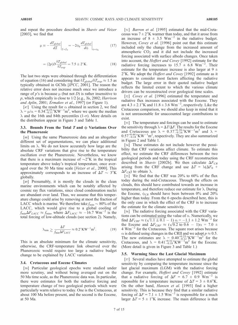
Figure 2. The probability distribution function for l (andDT�2) obtained by comparing radiation budget differencesto temperature change over various time scales, assumingthat CRF variations do not affect the global climate (thoughit does includes the small solar luminosity changes). Wealso assume, as Gregory et al. [2002], that DT and DFentering l have Gaussian errors. The cases are as follows:(1) temperature increase over the past century (followingGregory et al. [2002]), (2) temperature variations over300 years of solar cycles, (3) warming since the LGM(following Hoffert and Covey [1992] and Hansen et al.[1993]), (4) cooling relative to the Cretaceous (�100 Ma[Hoffert and Covey, 1992]), (5) cooling relative to theEocene (�55 Ma, following Covey et al. [1996]), and(6) Phanerozoic DT versus RCO2 (section 3.1, followingShaviv and Veizer [2003]). We assume that the temperatureincrease DT�2 following the doubling of the atmosphericCO2 content corresponds to an increase of 3.71 Wm�2

[Myhre et al., 1998].

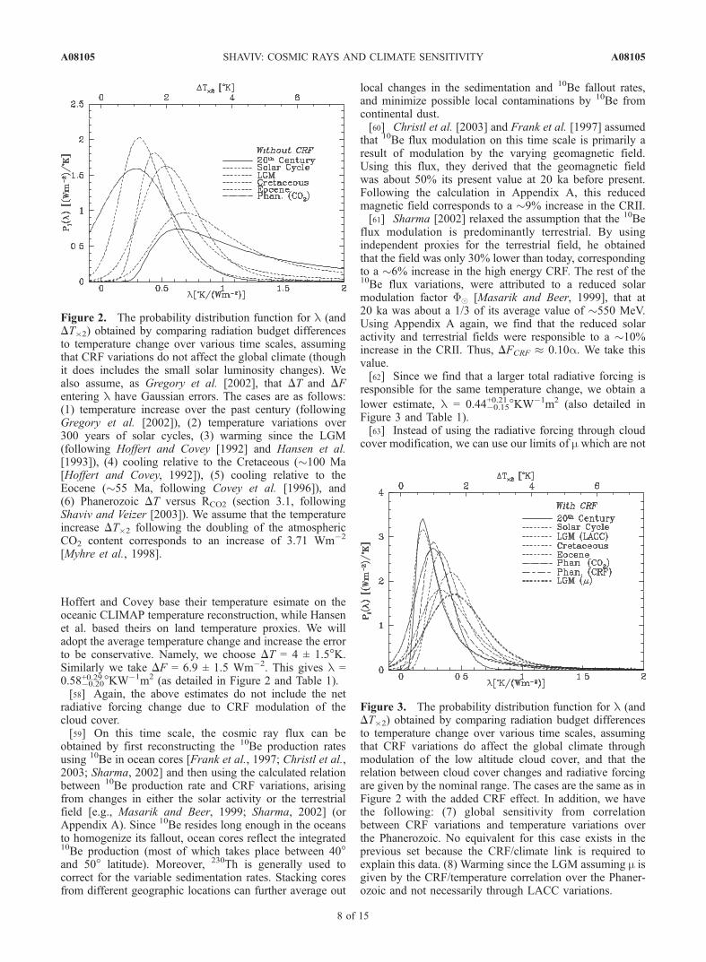
Figure 3. The probability distribution function for l (andDT�2) obtained by comparing radiation budget differencesto temperature change over various time scales, assumingthat CRF variations do affect the global climate throughmodulation of the low altitude cloud cover, and that therelation between cloud cover changes and radiative forcingare given by the nominal range. The cases are the same as inFigure 2 with the added CRF effect. In addition, we havethe following: (7) global sensitivity from correlationbetween CRF variations and temperature variations overthe Phanerozoic. No equivalent for this case exists in theprevious set because the CRF/climate link is required toexplain this data. (8) Warming since the LGM assuming m isgiven by the CRF/temperature correlation over the Phaner-ozoic and not necessarily through LACC variations.


8 of 15

A08105

based on LACC forcing, but instead on the observedtemperature change over the phanerozoic. We found m =7.5 ± 2�K. Thus, the 10% decrease in the CRII causing lowaltitude tropospheric ionization should translate into acontribution of DTCRF � 0.75 to 0.2�K. Next, the sensitivityrelation gives DT = l(DF0 + DFCRF) � lDF0 + DTCRF, andthereby obtain: l = 0.48�0.20

+0.27 �KW�1m2.[64] To summarize, the effect of the decreased CRF since

the LGM is to reduce our estimate for l by about 20%,which is smaller than the error in the estimate itself. Thisresult is valid also if we do not believe the CRF-climate linkis through LACC moduation, but merely that such a linkexists.

3.6. Warming Over the Past Century

[65] Climate sensitivity can also be estimated using theglobal warming observed over the past century once theradiative forcing with their uncertainties are estimated.[66] Since the time scale is relatively short, it is necessary

to consider the finite heat capacity of the oceans. We baseour analysis here on the work of Gregory et al. [2002], whotackled this problem by considering the heat flux into theocean in the energy budget. The main difference betweenour modified analysis here and that of Gregory et al. [2002],is that we will also consider the radiative forcing associatedwith the decreased CRF over the past century. Unlike thewarming since the LGM, where this was a small correction,here it is will prove to be a notable one.[67] Again, we assume that the CRF modulates the LACC

and that its radiative forcing is given in section 2.[68] Gregory et al. [2002] compared the period 1850–

1900 with 1950–1990. Since the CRF record does not goback far enough, we need to use 10Be as proxy data, which isknown to be a good proxy of solar activity [e.g., Lockwood,2001, 2003; Usoskin et al., 2002]. Using the Dye 3 record,the average 10Be flux appears to have decreased from about1.1 to 0.7 � 104atoms g�1 between the former and latterperiods [Beer, 2000; McCracken et al., 2004]. Using thecalculation in Appendix A, this reduction in 10Be, implies areduction of about 6% in the CRII. Using our estimate forthe radiative forcing change in section 2, this corresponds toa forcing of about 1.3 ± 0.5Wm�2.[69] According to Gregory et al. [2002],

lDT ¼ F � Q; ð20Þ

where F is the change in the radiative forcing (i.e., in theenergy balance), while Q is the average net heat flux whichentered the oceans between the two periods.[70] In our modified case F = F0 + FCRF, where F0 is the

‘‘standard’’ radiative forcing that was estimated by Gregoryet al. [2002] to be F0 = �0.3 to 1 Wm�2. It includesanthropogenic, volcanic, solar luminosity and aerosolcontributions (with the last one contributing the largestuncertainty). Q was estimated to be 0.32 ± 0.15 Wm�2

while DT = 0.335 ± 0.033�K (all at 2s).[71] Like Gregory et al. [2002], we assume that the errors

have a Gaussian distribution. Following their procedure, wecalculate the probability distribution function (PDF) for l.They are given in Figures 2 and 3 for the CRF and no-CRFcases. The added complication in the CRF case is the extraPDF for a, which implies that FCRF has a PDF itself. The

PDF obtained for the FCRF = 0 case is the same as the resultof Gregory et al. [2002].[72] Inspection of Figure 3 and Table 1 reveals that l =

0.27�0.10+0.32 �KW�1m2 at 1-s confidence. This is a clear

reduction from the results of Gregory et al. [2002], wherethe lower 16th percentile for l is 0.67�KW�1m2 and there isno formal upper limit. (This assumes a prior that l cannotbe negative.)

3.7. Variations Over the Solar Cycle

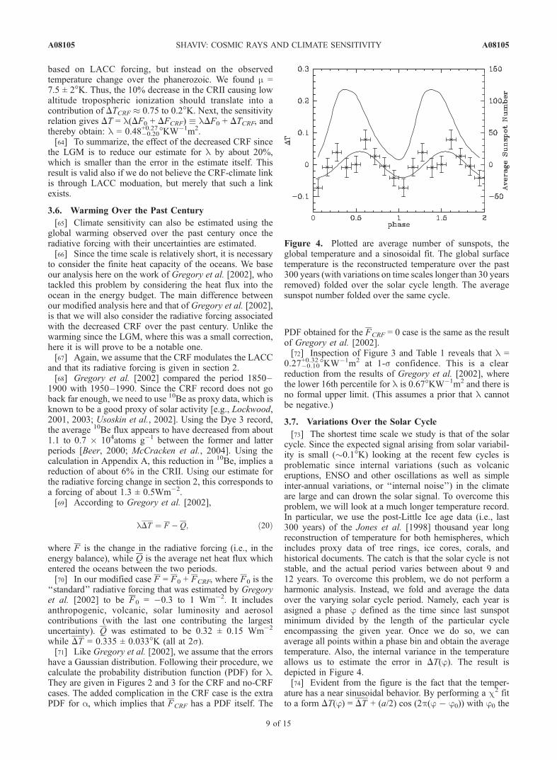
[73] The shortest time scale we study is that of the solarcycle. Since the expected signal arising from solar variabil-ity is small (�0.1�K) looking at the recent few cycles isproblematic since internal variations (such as volcaniceruptions, ENSO and other oscillations as well as simpleinter-annual variations, or ‘‘internal noise’’) in the climateare large and can drown the solar signal. To overcome thisproblem, we will look at a much longer temperature record.In particular, we use the post-Little Ice age data (i.e., last300 years) of the Jones et al. [1998] thousand year longreconstruction of temperature for both hemispheres, whichincludes proxy data of tree rings, ice cores, corals, andhistorical documents. The catch is that the solar cycle is notstable, and the actual period varies between about 9 and12 years. To overcome this problem, we do not perform aharmonic analysis. Instead, we fold and average the dataover the varying solar cycle period. Namely, each year isasigned a phase j defined as the time since last sunspotminimum divided by the length of the particular cycleencompassing the given year. Once we do so, we canaverage all points within a phase bin and obtain the averagetemperature. Also, the internal variance in the temperatureallows us to estimate the error in DT(j). The result isdepicted in Figure 4.[74] Evident from the figure is the fact that the temper-

ature has a near sinusoidal behavior. By performing a c2 fitto a form DT(j) = DT + (a/2) cos (2p(j � j0)) with j0 the

Figure 4. Plotted are average number of sunspots, theglobal temperature and a sinosoidal fit. The global surfacetemperature is the reconstructed temperature over the past300 years (with variations on time scales longer than 30 yearsremoved) folded over the solar cycle length. The averagesunspot number folded over the same cycle.


9 of 15

A08105

phase relative to the occurrence of maximum sunspotnumber, we find at the 1-s confidence limit that:

a ¼ 0:09� 0:03�K; ð21Þ

j0 ¼ 1:0� 0:6 rad: ð22Þ

The value of j0 implies that the average temperature lagsbehind the maximum sunspot number by 1.8 ± 1.0 years.This is to be expected, because of Earth’s finite heatcapacity. As a result, the response to radiative perturbationsis not only damped, but it is lagged as well.[75] Other analyses estimated the surface temperature

variation over the 11-yr solar cycle. Douglass and Clader[2002] found a = 0.11 ± 0.02�K, while White et al. [1997]found a = 0.10 ± 0.02�K. Together with the current result,we will adopt a = 0.10 ± 0.02�K for the temperaturevariation between solar minimum and solar maximum.[76] We now use the results of section 2. In particular,

the above temperature variations are assumed to arise fromthe �1.6% variations observed in the LACC, such that theforcing over the solar cycle is DFLACC = 1.0 ± 0.4 Wm�2.An additional contribution of DFflux = 0.35 Wm�2 is dueto changes in the solar flux. The sensitivity itself is thengiven by

l ¼ DT=d

DFð23Þ

where d is a damping factor which arises from the finite heatcapacity of the climate system and its inability to reachequilibrium at a finite time.[77] The value of the damping factor is not well known.

In principle, it can be obtained in climate models, but thesegive a range of values. Using a simple ocean/climate model,M. E. Schlesinger et al. (On the use of autoregressionmodels to estimate climate sensitivity, submitted to ClimateChange, 2004) (hereinafter referred to as Schlesinger et al.,submitted manuscript, 2004) obtained a damping of about0.25 on the 11-yr solar cycle time scale (and about 0.75 onthe centennial time scale). Other more extensive simulationsfind that the 11-yr solar cycle is damped relative to thecentennial scale by a factor of �0.54 [Cubasch et al., 1997],0.33 [Rind et al., 1999] or by comparing solar forcing toactual climate responce, to �0.68 [Waple et al., 2002]. If wefurther consider that the centennial time scale is dampedrelative to the long term response, by a factor of �0.7–0.75[IPCC, 2001; Schlesinger et al., submitted manuscript,2004], then the 4 estimates for the damping factor areencompassed within d = 0.35 ± 0.15, for periodic oscilla-tions with an 11-yr period.[78] Note that by resorting to GCMs for the estimate of

the damping factor, we are somewhat unfaithful to the spiritof this work, which is to estimate the sensitivity indepen-dently to the usage of GCM simulations. Nevertheless, thedamping we use is a characteristic describing the relativebehavior of different time scales. We still avoid using theabsolute sensitivity obtained in GCMs. Moreover, theanalysis of Waple et al. [2002] does indicate that empiri-cally, the damping factor is consistent with that obtained in

GCMs. The fact that this result is somewhat larger thanGCMs on average, would imply that we maybe under-estimating the damping factor, and with it, overestimatingthe climate sensitivity.[79] For the above nominal values of DT, DF and d,

equation (23) yields that l = 0.26�0.11+0.26 �KW�1m2. Without

the effects of the CRF, a much larger sensitivity (of l =0.94�0.35

+0.91 �KW�1m2) is obtained because the same temper-ature variations are then to be explained only by therelatively small solar flux variations.

3.8. Combined Results

[80] We now proceed to combine the PDFs obtained inthe cases described in Figure 2, when the CRF/climate linkis neglected, and the cases described in Figure 3, when theCRF/LACC effect is included. We combine the results intwo cases. In the first, we assume that the global temper-ature sensitivity is constant, namely, that it does not dependon the average terrestrial temperature. In the second case,we allow the sensitivity to be temperature dependent.3.8.1. Constant Sensitivity[81] When combining the results under the assumption

that CRF does not introduce a radiative forcing, we cansimply multiply the PDFs and renormalize the result. Thereason is that the error in the estimates of all the DF0 and DTare presumably uncorrelated with each other, and alsobecause we have no prior on the value of l (except perhapsthat it should be positive).

Figure 5. The combined probability distribution functionsfor l obtained by combining the PDFs given in Figures 2and 3 when the CRF/climate link is either neglected orincluded. (In the latter case, the combination is done asexplained in the text.) Thin lines denote the result if l isassumed to be temperature insensitive, while the heavy lineis the result obtained when l is allowed to be a linearfunction of the temperature. The the latter case, thedistribution for l today is plotted. Also marked are thetwo additional constraints obtained from the Phanerozoicdata which do not depend on the CRF/LACC link, as wellas the sensitivity range of 1.5 to 4.5�K, which according toIPCC [2001] is ‘‘widely cited’’. Note that the sensitivityrange of the 15 GCM models actually used by the IPCC[2001] is 2.0 to 5.1�K.


10 of 15

A08105

[82] On the other hand, when combining the cases whichinclude the CRF/LACC effect, we must bear in mind thatsome of the error arises from the uncertainty in a: therelation between cloud cover changes and radiative forcing.This uncertainty enters 5 PDFs, and we cannot simplymultiply them. To overcome this obstacle, we calculatethe PDFs assuming a given a. Then, the combined PDFis given by

Pall lð Þ ¼

Z Y6

i¼1Pi l;að Þ

h iPa að ÞdaZ Y6

i¼1Pi l;að Þ

h iPa að Þdadl

: ð24Þ

Again, this assumes that we have no prior on l, and thatbesides the dependence on a, the PDFs are not in anywaycorrelated with each other.[83] In Figures 5 and 7 and Table 1, we plot and describe

the combined PDFs obtained in the two cases. We find thatl = 0.52�0.08

+0.10 �KW�1m2 if the CRF/climate link is neglected,and that l = 0.28�0.05

+0.07 �KW�1m2 if the CRF/LACC link isincluded. Values of upper and lower limits on l and DT�2 atdifferent confidence limits are given in Table 1.3.8.2. Variable Sensitivity[84] We now alleviate the assumption of a constant

sensitivity and allow a linear relation of the form l =

l0 + bDT, where l0 is the sensitivity today and b = dl/dT.Because the errors are not Gaussian (the distributionsare generally skewed towards higher l’s) we cannot fitl(DT) using a simple linear least squares. Instead, wecalculate

Pall l0; bð Þ ¼

Z Y6

i¼1Pi l0 þ bDTi;að Þ

h iPa að ÞdaZ Y6

i¼1Pi l0 þ bDTi;að Þ

h iPa að Þdadldb

; ð25Þ

and Pall(l0) =RPall(l0, b) db.

[85] Here we find that l = 0.54�0.10+0.12 �KW�1m2 if the CRF/

climate link is neglected, and that l = 0.34�0.08+0.10 �KW�1m2 if

the CRF/LACC link is included. Values of upper and lowerlimits on l and DT�2 at different confidence limits are givenin Table 1.[86] This is our best estimate for the global sensitivity. It

translates into a CO2 doubling temperature change ofDT�2 = 1.3 ± 0.3�K. With the CRF/climate effectneglected, this number is DT�2 = 2.0 ± 0.5�K.[87] Another point worth mentioning is the fact that once

the CRF/LACC climate link is included, the median valuesfor l obtained using different periods differ from each otherby typically 1-s or less, while without the CRF/climateconsidered, differences can be larger than 2-s. Namely, the

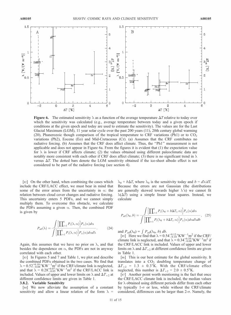
Figure 6. The estimated sensitivity l as a function of the average temperature DT relative to today overwhich the sensitivity was calculated (e.g., average temperature between today and a given epoch ifconditions at the given epoch and today are used to estimate the sensitivity). The values are for the LastGlacial Maximum (LGM), 11 year solar cycle over the past 200 years (11), 20th century global warming(20), Phanerozoic though comparison of the tropical temperature to CRF variations (Ph1) or to CO2

variations (Ph2), Eocene (Eo) and Mid-Cretaceous (Cr). (a) Assumes that the CRF contributes noradiative forcing. (b) Assumes that the CRF does affect climate. Thus, the ‘‘Ph1’’ measurement is notapplicable and does not appear in Figure 6a. From the figures it is evident that (1) the expectation valuefor l is lower if CRF affects climate; (2) the values obtained using different paleoclimatic data arenotably more consistent with each other if CRF does affect climate; (3) there is no significant trend in lversus DT. The dotted bars denote the LGM sensitivity obtained if the ice-sheet albedo effect is notconsidered to be part of the radiative forcing (see section 4).


11 of 15

A08105

CRF/climate effect markably improves the consistency ofthe data. This can be seen in Figure 6.

4. Discussion

[88] We compared the radiative forcing and temperaturechange over several different time scales, while taking intoconsideration the alleged link between CRF variations andtemperature change. We found that the 6 different time scalescan be used to place similar bound on the global climatesensitivity and, when possible, also on the quantitativerelation between CRF variations and temperature change.[89] Before continuing with a discussion of the different

caveats and implications of the results obtained, we shouldcarefully consider the meaning of the sensitivity calculated.Specifically, the sensitivity calculated was obtained throughthe comparison of radiative forcings to temperature re-sponse. However, in some cases, it is not clear whether aradiative forcing should be considered as part of the re-sponse of the system or part of the drivers. For the 11-yrsolar cycle and the Phanerozoic-DT/Df comparisons, it isclear we are considering only ‘‘external’’ forcings andeverything terrestrial is part of the system. In the Phanero-zoic-DT/CO2 and 20th century warming, the ‘‘external’’drivers also include variation in the greenhouse gasses(excluding water vapor). We explicitly assumed that theyare not part of the system but are externally forced, forexample, through tectonic activity in the geological case oranthropogenic over the 20th century.[90] The case of the LGM comparison, and to a notably

smaller extent, the Cretaceous and Eocene comparisons,

include changes associated with changes in the extent of theice-sheets. In principle, these can be considered as externaldrivers or as an integral part of the system. In the LGMcalculation, for example, the LGM radiative forcing of7Wm�2 [Hansen et al., 1993] we used, includes about2Wm�2 due to ice-sheet albedo effects. If we allow theice-sheet changes to be part of the response of the system,then the sensitivity obtained from the LGM is notablyhigher, being l = 0.56�0.20

+0.28 �KW�1m2. Thus, the sensitivitywe used in the analysis does not include the response of thecryosphere. For cold climates (i.e., colder than today) wewould underestimate the sensitivity if the cryosphere isallowed to be part of the system.[91] Other than the important point above, we should also

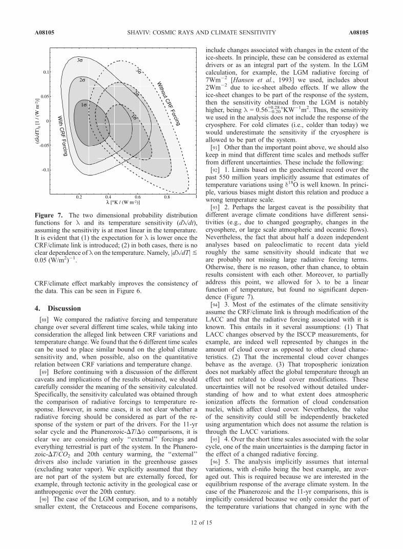
keep in mind that different time scales and methods sufferfrom different uncertainties. These include the following:[92] 1. Limits based on the geochemical record over the

past 550 million years implicitly assume that estimates oftemperature variations using d18O is well known. In princi-ple, various biases might distort this relation and produce awrong temperature scale.[93] 2. Perhaps the largest caveat is the possibility that

different average climate conditions have different sensi-tivities (e.g., due to changed geography, changes in thecryosphere, or large scale atmospheric and oceanic flows).Nevertheless, the fact that about half a dozen independentanalyses based on paleoclimatic to recent data yieldroughly the same sensitivity should indicate that weare probably not missing large radiative forcing terms.Otherwise, there is no reason, other than chance, to obtainresults consistent with each other. Moreover, to partiallyaddress this point, we allowed for l to be a linearfunction of temperature, but found no significant depen-dence (Figure 7).[94] 3. Most of the estimates of the climate sensitivity

assume the CRF/climate link is through modification of theLACC and that the radiative forcing associated with it isknown. This entails in it several assumptions: (1) ThatLACC changes observed by the ISCCP measurements, forexample, are indeed well represented by changes in theamount of cloud cover as opposed to other cloud charac-teristics. (2) That the incremental cloud cover changesbehave as the average. (3) That tropospheric ionizationdoes not markably affect the global temperature through aneffect not related to cloud cover modifications. Theseuncertainties will not be resolved without detailed under-standing of how and to what extent does atmosphericionization affects the formation of cloud condensationnuclei, which affect cloud cover. Nevertheless, the valueof the sensitivity could still be independently bracketedusing argumentation which does not assume the relation isthrough the LACC variations.[95] 4. Over the short time scales associated with the solar

cycle, one of the main uncertainties is the damping factor inthe effect of a changed radiative forcing.[96] 5. The analysis implicitly assumes that internal

variations, with el-nino being the best example, are aver-aged out. This is required because we are interested in theequilibrium response of the average climate system. In thecase of the Phanerozoic and the 11-yr comparisons, this isimplicitly considered because we only consider the part ofthe temperature variations that changed in sync with the

Figure 7. The two dimensional probability distributionfunctions for l and its temperature sensitivity (dl/dt),assuming the sensitivity is at most linear in the temperature.It is evident that (1) the expectation for l is lower once theCRF/climate link is introduced; (2) in both cases, there is noclear dependence of l on the temperature. Namely, jdl/dTj]0.05 (W/m2)�1.


12 of 15

A08105

radiative forcing. Thus, by definition, internal oscillations orrandomness are averaged out. The 20th century warmingfollows the analysis of Gregory et al. [2002], whodecoupled the atmospheric from the oceanic componentsby explicitly considering the heat transfer to the oceans.Since the atmosphere is not expected to have internaldynamics (without external forcing) on this time scale, allsuch internal contributions are presumably averaged out.The three other comparisons are the climate variations sincethe mid-Cretaceous, the Eocene and the LGM. Here randomor oscillatory long term internal variations of the systemcould in principle exist and possibly affect the sensitivityestimate.[97] 6. We implicitly assumed here that climate sensitiv-

ity to changes in the cosmic ray flux remained constantthroughout the ages, under varying climatic and geographicconditions. This, however, is not automatically guaranteed,since the link was calibrated under Holocene conditions.Over time, for example, there could have been a change inthe average amount of water vapor in the atmosphere,governed by the average temperature, or the fraction andgeographic distribution of the landmass from which CCNthat are unrelated to atmospheric ionization, can originate.Thus, it is not unreasonable for there to have beenvariations in the quantitative link between CRF variationsand changes to the radiation budget. Without a betterunderstanding of the physical mechanism governing thelink, this assumption should therefore only be consideredas a working hypothesis.[98] 7. In the analysis, the sensitivity was obtained

either by considering small ‘‘perturbations’’ around Holo-cene type conditions, or, through comparison of largelydifferent climates. Thus, it is not unlikely that we aremissing climate instabilities which arise when consideringsmall variations around average conditions different thantoday. As an illustration, a prominent ocean current likethe gulf stream could switch on or off around averageconditions different than today. Not only would ourestimate for l be wrong in this case, the system mayhave complicated nonlinear dynamics that cannot even bedescribed with an effective l, such as a memory effect(e.g., hysteresis).[99] Having listed the caveats, it should also be noted that

once the CRF/climate effect is taken into account, anagreement between the sensitivities obtained. Not only doesit indicate that we are probably not missing unaccountedfactors, it provides another indicator that the CRF/climateeffect is real (see Figure 6a versus Figure 6b).[100] Our best estimate is DT�2 � 1.3 ± 0.3�K. This is at

the lower end of the often quoted range of DT�2 = 1.5 to4.5�K [IPCC, 2001] obtained from Global CirculationModels (GCMs). Cess et al. [1989] have shown that theclimate sensitivity obtained in this type of simulationspredominantly depends on how clouds are treated, andwhether they contribute a positive or negative feedback.The models roughly give that l�1 � 2.2 Wm�2/�K �DFcloud/D�T with DFcloud being the feedback forcing ofclouds associated with a temperature change of D�T . Thus,for a GCM to be compatible with the results obtained here, anegative cloud feedback is required. One such example wassuggested by Lindzen et al. [2001].

[101] On the other side of the coin, we can also rule outvery small climate sensitivities. This can be used forexample to place a limit on possible large negative feed-backs, or to a lower limit on the effect of anthropogenicgreenhouse gas (GHG) warming.[102] Since the beginning of the industrial era (�1750),

non-solar sources contributed a net forcing of 0.85 ±1.3 Wm�2 [IPCC, 2001] (assuming the errors are Gaussian).Over the past century alone, this number is 0.5 ± 1.3 Wm�2.The main reason why the error is large is because of theuncertain ‘‘indirect’’ contribution of aerosols, namely, theireffect on cloud cover. It is currently estimated to be in therange �1 ± 1 Wm�2 [IPCC, 2001]. Thus, anthropogenicsources alone contributed to a warming of 0.14 ± 0.36�Ksince the beginning of the 20th century.[103] The sensitivity result can also be used to estimate

the solar contribution towards global warming. Over thepast century, the increased solar activity has been responsi-ble for a stronger solar wind and a lower CRF. Using resultsof section 3.6, the reduced ionization and LACC wereresponsible for an increased radiative forcing of 1.3 ±0.5 Wm�2. In addition, the globally averaged solar lumi-nosity increased by about 0.4 ± 0.1 Wm�2 according toSolanki and Fligge [1998], Hoyt and Schatten [1993], andLean et al. [1995]. Thus, increased solar activity is respon-sible for a total increase of 1.7 ± 0.6 Wm�2. Using ourestimate for l, we find DTsolar = 0.47 ± 0.19�K.[104] We therefore find that the combined solar and

anthropogenic sources were responsible for an increase of0.61 ± 0.42�K. This should be compared with the observed0.57 ± 0.17�K increase in global surface temperature [IPCC,2001]. In other words, the result we find for the sensitivityand drivers are consistent with the observed temperatureincrease. This conclusion, about the relative role of solarversus anthropogenic sources was independently reached bycomparing the non-monotonic temperature increase with thenon-monotonic solar activity increase and the monotonicincrease in GHGs [Soon et al., 1996b].

Appendix A

[105] Over geological time scales, both a galactic cosmicray diffusion model and a record in Iron meteorites can beindependently used to estimate CRF and atmospheric ion-ization rate changes. On shorter time scales, of a few 100 kaor shorter, we need another method. 10Be is sensitive to thevarying CRF and can be reconstructed using ice-cores andsea floor sediments. However, the energy sensitivity isdifferent than that of atmospheric ionization: 10Be is formedby CRs which are on average less energetic than the CRsresponsible for the atmospheric ionization. Thus, using the10Be record to reconstruct the atmospheric ionization ispossible but it requires correcting for the different energysensitivity.[106] We calculate here the sensitivity of the atmospheric

ionization rate to changes in the CRs which arise fromchanges in solar activity (as encompassed in the solarmodulation parameter F�) and changes in the terrestrialmagnetic field strength m as compared to the field today. Wewill compare those to the production rate of 10Be as afunction of both parameters.


13 of 15

A08105

[107] The flux of cosmic rays reaching 1 AU depends onthe solar modulation parameter. It is given by [Masarik andBeer, 1999]:

J E;F�ð Þ ¼ Cp

Ep Ep þ 2mpc2

�Ep þ xþ F� ��2:5

Ep þ F� �

Ep þ 2mpc2 þ F� � ; ðA1Þ

with x = (780 MeV) exp (�2.5 � 10�4Ep/MeV) and C =1.24 � 106 cm�2 s�1MeV�1. Frfsom these cosmic rays, theparticles which can actually reach the atmosphere and notbe cut off by the magnetic field, at latitude J, are those witha rigidity above the cutoff, given by

Pc Jð Þ � 14:8GVð Þ cos4 Jð Þ m=m0ð Þ; ðA2Þ

where m is the geomagnetic dipole moment, and m0 = 7.8 �1025 G cm3 is the current day dipole.[108] Masarik and Beer [1999] used these expressions

and the various spallation cross-sections to obtain theglobally averaged production rate of 10Be as a function ofF� and m. Their results were analytically fitted by Sharma[2002]. Thus, given changes in F� and m, relative to theirrecent averages, the change in the 10Be production rate canbe straightforwardly obtained.[109] The next step is to use the ionization yield to obtain

to total ionization rate from the flux which can actuallyreach the atmosphere. We use the ionization yields calcu-lated by Usoskin et al. [2004b]. These are given as Y(E, h),the total ionization at height h arising from a cosmic ray at

energy E. We take the average ionization between 0 and3 km, the altitude of LACC.[110] To obtain the actual ionization rate R, we integrate:

R m;F�;Jð Þ ¼Z 1

Pc

J E;F�ð ÞY E;Jð ÞdE: ðA3Þ

[111] Empirically, it appears that cloud cover is propor-tional to the density of atmospheric ions [Usoskin et al.,2004a], while the latter is proportional to the relative change

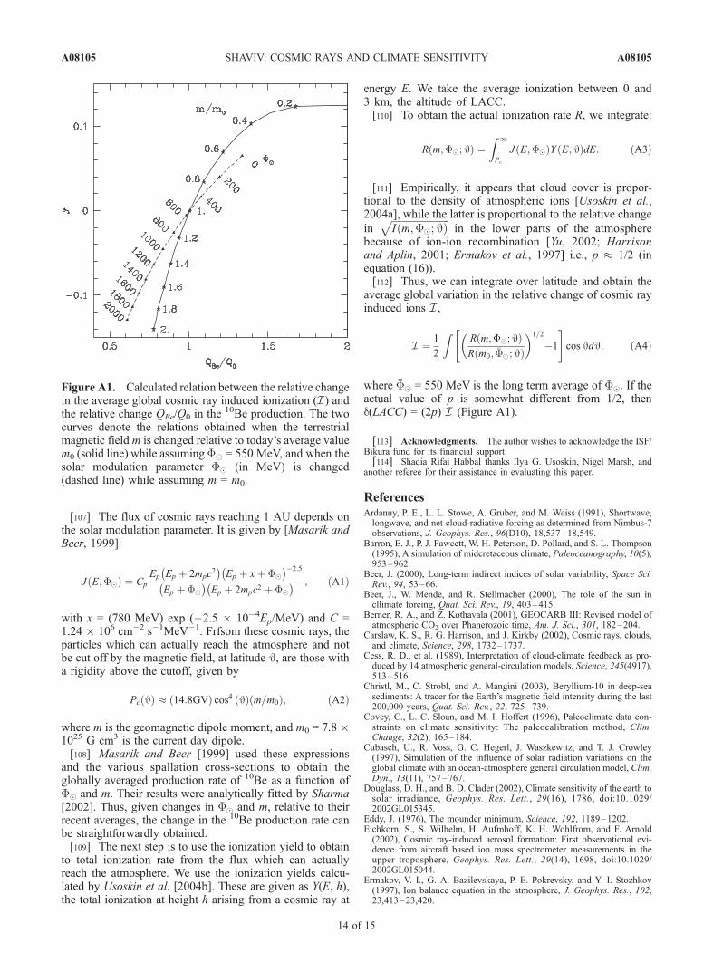
inffiffiffiffiffiffiffiffiffiffiffiffiffiffiffiffiffiffiffiffiffiffiffiI m;F�;Jð Þ

pin the lower parts of the atmosphere

because of ion-ion recombination [Yu, 2002; Harrisonand Aplin, 2001; Ermakov et al., 1997] i.e., p � 1/2 (inequation (16)).[112] Thus, we can integrate over latitude and obtain the

average global variation in the relative change of cosmic rayinduced ions I ,

I ¼ 1

2

ZR m;F�;Jð ÞR m0; �F�;Jð Þ

� �1=2

�1

" #cosJdJ; ðA4Þ

where �F� = 550 MeV is the long term average of F�. If theactual value of p is somewhat different from 1/2, thend(LACC) = (2p) I (Figure A1).

[113] Acknowledgments. The author wishes to acknowledge the ISF/Bikura fund for its financial support.[114] Shadia Rifai Habbal thanks Ilya G. Usoskin, Nigel Marsh, and

another referee for their assistance in evaluating this paper.

ReferencesArdanuy, P. E., L. L. Stowe, A. Gruber, and M. Weiss (1991), Shortwave,longwave, and net cloud-radiative forcing as determined from Nimbus-7observations, J. Geophys. Res., 96(D10), 18,537–18,549.

Barron, E. J., P. J. Fawcett, W. H. Peterson, D. Pollard, and S. L. Thompson(1995), A simulation of midcretaceous climate, Paleoceanography, 10(5),953–962.

Beer, J. (2000), Long-term indirect indices of solar variability, Space Sci.Rev., 94, 53–66.

Beer, J., W. Mende, and R. Stellmacher (2000), The role of the sun incllimate forcing, Quat. Sci. Rev., 19, 403–415.

Berner, R. A., and Z. Kothavala (2001), GEOCARB III: Revised model ofatmospheric CO2 over Phanerozoic time, Am. J. Sci., 301, 182–204.

Carslaw, K. S., R. G. Harrison, and J. Kirkby (2002), Cosmic rays, clouds,and climate, Science, 298, 1732–1737.

Cess, R. D., et al. (1989), Interpretation of cloud-climate feedback as pro-duced by 14 atmospheric general-circulation models, Science, 245(4917),513–516.

Christl, M., C. Strobl, and A. Mangini (2003), Beryllium-10 in deep-seasediments: A tracer for the Earth’s magnetic field intensity during the last200,000 years, Quat. Sci. Rev., 22, 725–739.

Covey, C., L. C. Sloan, and M. I. Hoffert (1996), Paleoclimate data con-straints on climate sensitivity: The paleocalibration method, Clim.Change, 32(2), 165–184.

Cubasch, U., R. Voss, G. C. Hegerl, J. Waszkewitz, and T. J. Crowley(1997), Simulation of the influence of solar radiation variations on theglobal climate with an ocean-atmosphere general circulation model, Clim.Dyn., 13(11), 757–767.

Douglass, D. H., and B. D. Clader (2002), Climate sensitivity of the earth tosolar irradiance, Geophys. Res. Lett., 29(16), 1786, doi:10.1029/2002GL015345.

Eddy, J. (1976), The mounder minimum, Science, 192, 1189–1202.Eichkorn, S., S. Wilhelm, H. Aufmhoff, K. H. Wohlfrom, and F. Arnold(2002), Cosmic ray-induced aerosol formation: First observational evi-dence from aircraft based ion mass spectrometer measurements in theupper troposphere, Geophys. Res. Lett., 29(14), 1698, doi:10.1029/2002GL015044.

Ermakov, V. I., G. A. Bazilevskaya, P. E. Pokrevsky, and Y. I. Stozhkov(1997), Ion balance equation in the atmosphere, J. Geophys. Res., 102,23,413–23,420.

Figure A1. Calculated relation between the relative changein the average global cosmic ray induced ionization (I ) andthe relative change QBe/Q0 in the 10Be production. The twocurves denote the relations obtained when the terrestrialmagnetic field m is changed relative to today’s average valuem0 (solid line) while assuming F� = 550 MeV, and when thesolar modulation parameter F� (in MeV) is changed(dashed line) while assuming m = m0.


14 of 15

A08105

Farrar, P. D. (2000), Are cosmic rays influencing oceanic cloud coverage -or is it only El Nino?, Clim. Change, 47(1–2), 7–15.

Frank, M., B. Schwarz, S. Baumann, P. W. Kubik, M. Suter, and A. Mangini(1997), A 200 kyr record of cosmogenic radionuclide production rateand geomagnetic field intensity from Be-10 in globally stacked deep-sea sediments, Earth Planet. Sci. Lett., 149, 121–129.

Friis-Christensen, E., and K. Lassen (1991), Length of the solar cycle: Anindicator of solar activity closely associated with climate, Science, 254,698.

Frohlich, C., and J. Lean (1998), The sun’s total irradiance: Cycles, trendsand related climate change uncertainties since 1976, Geophys. Res. Lett.,25(23), 4377–4380.

Gregory, J. M., R. J. Stouffer, S. C. B. Raper, P. A. Stott, and N. A. Rayner(2002), An observationally based estimate of the climate sensitivity,J. Clim., 15, 3117–3121.

Hansen, J., A. Lacis, R. Ruedy, M. Sato, and H. Wilson (1993), Howsensitive is the worlds climate, Res. Explor., 9(2), 142–158.

Hansen, J. E., M. Sato, A. Lacis, R. Ruedy, I. Tegen, and E. Matthews(1998), Climate forcings in the industrial era, Proc. Natl. Acad. Sci., 95,12,753–12,758.

Harrison, R. G., and K. L. Aplin (2001), Atmospheric condensation nucleiformation and high-energy radiation, J. Atmos. Terr. Phys., 63, 1811–1819.

Hartmann, D. L., M. E. Ockert-Bell, and M. L. Michelsen (1992), Theeffect of cloud type on Earth’s energy balance: Global analysis, J. Clim.,5, 128.

Herschel, W. (1796), Some remarks on the stability of the light of the sun,Philos. Trans. R. Soc. London, 0, 166.

Hobbs, P. (1993), Aerosol-cloud interactions, in Aerosol-Cloud-ClimateInteractions., Int. Geophys. Ser., vol. 54, Elsevier, New York.

Hodell, D. A., M. Brenner, J. H. Curtis, and T. Guilderson (2001), Solarforcing of drought frequency in the maya lowlands, Science, 292, 1367–1370.

Hoffert, M. I., and C. Covey (1992), Deriving global climate sensitivityfrom paleoclimate reconstructions, Nature, 360(6404), 573–576.

Hoyt, D. V., and K. H. Schatten (1993), A discussion of plausible solarirradiance variations, 1700–1992, J. Geophys. Res., 98(A11), 18,895–18,906.

Intergovernmental Panel on Climate Change (IPCC) (2001), ClimateChange 2001, Cambridge Univ. Press, New York.

Jones, P. D., K. R. Briffa, T. P. Barnett, and S. F. B. Tett (1998), High-resolution palaeoclimatic records for the last millennium: Interpretation,integration and comparison with general circulation model control-runtemperatures, Holocene, 8(4), 455–471.

Kirkby, J., and A. Laaksonen (2000), Solar Variability and Clouds - Dis-cussion Session 3c, Space Sci. Rev., 94, 397–409.

Labitzke, K., and H. van Loon (1992), J. Clim, 5, 240.Lavielle, B., K. Marti, J. Jeannot, K. Nishiizumi, and M. Caffee (1999), The

36Cl-36Ar-40K-41K records and cosmic ray production rates in iron me-teorites, Earth Planet. Sci. Lett., 170, 93–104.

Lean, J., J. Beer, and R. Bradley (1995), Reconstruction of solar irradiancesince 1610 - Implications for climate change, Geophys. Res. Lett., 22(23),3195–3198.

Lindzen, R. S., M.-D. Chou, and A. Y. Hou (2001), Does the Earth have anadaptive infrared iris?, Bull. Am. Meteorol. Soc., 82, 417–431.

Lockwood, M. (2001), Long-term variations in the magnetic fields of theSun and the heliosphere: Their origin, effects, and implications, J. Geo-phys. Res., 106(A8), 16,021.

Lockwood, M. (2003), Twenty-three cycles of changing open solar mag-netic flux, J. Geophys. Res., 108(A3), 1128, doi:10.1029/2002JA009431.

Marsden, D., and R. E. Lingenfelter (2003), Solar activity and cloud opa-city variations: A modulated cosmic ray ionization model, J. Atmos. Sci.,60(4), 626–636.

Marsh, N., and H. Svensmark (2000a), Cosmic rays, clouds, and climate,Space Sci. Rev., 94, 215–230.

Marsh, N., and H. Svensmark (2000b), Low cloud properties influenced bycosmic rays, Phys. Rev. Lett., 85, 5004–5007.

Marsh, N., and H. Svensmark (2003), Galactic cosmic ray and El Nino–Southern Oscillation trends in International Satellite Cloud ClimatologyProject D2 low-cloud properties, J. Geophys. Res., 108(D6), 4195,doi:10.1029/2001JD001264.

Masarik, J., and J. Beer (1999), Simulation of particle fluxes and cosmo-genic nuclide production in the Earth’s atmosphere, J. Geophys. Res.,104, 12,099–12,111.

McCracken, K. G., J. Beer, and F. B. McDonald (2004), Variations in thecosmic radiation, 1890–1986, and the solar and terrestrial implications,Adv. Space Res., 34, 397–406.

Myhre, G., E. J. Highwood, K. P. Shine, and F. Stordal (1998), Newestimates of radiative forcing due to well mixed greenhouse gases, Geo-phys. Res. Lett., 25, 2715.

Neff, U., S. J. Burns, A. Mangnini, M. Mudelsee, D. Fleitmann, andA. Matter (2001), Strong coherence between solar variability and themonsoon in oman between 9 and 6 kyr ago, Nature, 411, 290–293.

Ney, E. P. (1959), Cosmic radiation and weather, Nature, 183, 451.Palle Bago, E., and J. Butler (2000), The influence of cosmic terrestrialclouds and global warming, Astron. Geophys., 41, 18–22.

Rind, D., J. Lean, and R. Healy (1999), Simulated time-dependent climateresponse to solar radiative forcing since 1600, J. Geophys. Res., 104(D2),1973–1990.

Rosenfeld, D. (2000), Suppression of rain and snow by urban and industrialair pollution, Science, 287, 1793–1796.

Royer, D., R. Berner, I. Montanez, N. Tabor, and D. Beerling (2004), CO2

as a primary driver of phanerozoic climate, GSA Today, 14(3), 4–10.Sharma, M. (2002), Variations in solar magnetic activity during the last200,000 years: Is there a sun-climate connection?, Earth Planet. Sci.Lett., 199(3–4), 459–472.

Shaviv, N. J. (2002a), Cosmic ray diffusion from the galactic spiral arms,iron meteorites, and a possible climatic connection?, Phys. Rev. Lett., 89,051,102.

Shaviv, N. J. (2002b), The spiral structure of the Milky Way, cosmic rays,and ice age epochs on earth, New Astron., 8, 39–77.

Shaviv, N. J. (2003), Toward a solution to the early faint Sun paradox: Alower cosmic ray flux from a stronger solar wind, J. Geophys. Res.,108(A12), 1437, doi:10.1029/2003JA009997.

Shaviv, N. J., and J. Veizer (2003), A celestial driver of phanerozoic cli-mate?, GSA Today, 13(7), 4–11.

Shaviv, N., and J. Veizer (2004), Reply to Royer et al.’s letter ‘‘CO2 as aprimary driver of phanerozoic climate’’, GSA Today, 14(7), 18.

Solanki, S. K., and M. Fligge (1998), Solar irradiance since 1874 revisited,Geophys. Res. Lett., 25(3), 341–344.

Soon, W. H., E. S. Posmentier, and S. L. Baliunas (1996a), Inference ofsolar irradiance variability from terrestrial temperature changes, 1880–1993: An astrophysical application of the Sun-climate connection, Astro-phys. J., 472, 891.

Soon, W. H., E. S. Posmentier, and S. L. Baliunas (1996b), Inference ofsolar irradiance variability from terrestrial temperature changes, 1880–1993: An astrophysical application of the Sun-climate connection, Astro-phys. J., 472, 891.

Soon, W. H., E. S. Posmentier, and S. L. Baliunas (2000), Climate hyper-sensitivity to solar forcing?, Ann. Geophys., 18, 583+.

Stephens, G. L. (1978), Radiation profiles in extended water clouds. 2.Parameterization schemes, J. Atmos. Sci., 35(11), 2123–2132.

Svensmark, H. (1998), Influence of cosmic rays on earth’s climate, Phys.Rev. Lett., 81, 5027–5030.

Svensmark, H. (2000), Cosmic rays and earth’s climate, Space Sci. Rev., 93,175–185.

Twomey, S. (1977), The influence of pollution on the shortwave albedo ofclouds, J. Atmos. Sci., 34, 1149–1152.

Usoskin, I. G., K. Mursula, S. K. Solanki, M. Schussler, and G. A. Kovaltsov(2002), A physical reconstruction of cosmic ray intensity since 1610,J. Geophys. Res., 107(A11), 1374, doi:10.1029/2002JA009343.

Usoskin, I. G., N. Marsh, G. A. Kovaltsov, K. Mursula, and O. G.Gladysheva (2004a), Latitudinal dependence of low cloud amount oncosmic ray induced ionization, Geophys. Res. Lett., 31, L16109,doi:10.1029/2004GL019507.

Usoskin, I. G., O. G. Gladysheva, and G. A. Kovaltsov (2004b), Cosmicray-induced ionization in the atmosphere: Spatial and temporal changes,J. Atmos. Terr. Phys., 66, 1791–1796, doi:10.1016/j.jastp.2004.07.037.

Veizer, J., Y. Godderis, and L. M. Francois (2000), Evidence for decouplingof atmospheric CO2 and global climate during the phanerozoic eon,Nature, 408, 698.

Waple, A. M., M. E. Mann, and R. S. Bradley (2002), Long-term patterns ofsolar irradiance forcing in model experiments and proxy based surfacetemperature reconstructions, Clim. Dyn., 18(7), 563–578.

White, W. B., J. Lean, D. R. Cayan, and M. D. Dettinger (1997), Responseof global upper ocean temperature to changing solar irradiance, J. Geo-phys. Res., 102(C2), 3255–3266.

Yu, F. (2002), Altitude variations of cosmic ray induced production ofaerosols: Implications for global cloudiness and climate, J. Geophys.Res., 107(A7), 1118, doi:10.1029/2001JA000248.

��N. J. Shaviv, Racah Institute of Physics, Hebrew University of Jerusalem,

Jerusalem, 91904, Israel. ([email protected])


15 of 15

A08105

Documents

On climate response to changes in the cosmic ray flux and