Report - Ground clutter canceling with a regression filter

GROUND CLUTTER CANCELING WITH

A REGRESSION FILTER

National Severe Storms Laboratory Interim Report

prepared by: Sebastián Torres

with contributions by: Dusan S. Zrnic and R. J. Doviak

October 1998

NOAA, National Severe Storms Laboratory

1313 Halley Circle, Norman, Oklahoma 73069

Table of Contents 1. Preface............................................................................................................................. 1

2. Introduction..................................................................................................................... 2

3. Variable PRT Processing ................................................................................................ 3

4. Ground Clutter Filter....................................................................................................... 6

4.1. Orthogonal Polynomials ......................................................................................... 8

4.2. Regression Filters.................................................................................................... 9

4.3. Frequency Response of the Regression Filter....................................................... 12

5. Performance Analysis of the Regression Filter ............................................................ 18

5.1. Uniform PRT Scheme........................................................................................... 18

5.2. Application of filters to the WSR-88D data.......................................................... 26

5.3. Staggered PRT Scheme......................................................................................... 29

6. Future Work .................................................................................................................. 33

7. Conclusions................................................................................................................... 34

8. References..................................................................................................................... 36

1

1. Preface

This interim report documents part of accomplishments in the second year of the

MOU with the Operational Support Facility. The report explores filtering of ground

clutter in a staggered pulse repetition sequence. Specifically, a class of cancelers that use

regression is examined. Thus, first an expose of regression filters is presented and then

these are applied to a uniform PRT sequence. An extension to include staggered PRTs is

made and tested. Results on a uniform PRT sequence are quite good but do not yet carry

over to a staggered PRT. Approaches that might not degrade the spectral moment

estimates of staggered sequences are proposed.

2

2. Introduction

Weather radar data is often contaminated with unwanted returns from the ground.

Therefore, filtering techniques that attempt to ameliorate these signals are essential in

nearly all Doppler radar systems. If the clutter is not at least partially removed, it mimics

a meteorological signal and might produce strongly biased estimates of the three

fundamental physical parameters (mean power, mean Doppler velocity, and spectrum

width). In most cases, ground clutter signals have a very narrow spectrum width (long

correlation time) and their mean Doppler velocity is zero. Thus, a high percentage of this

interfering signal can be reduced if the spectral components in a band centered at zero

frequency (zero Doppler velocity) are removed by using a suitable high-pass filter.

Ground clutter filters with sharp narrow notches have been successfully designed and

implemented in the WSR-88D to operate on uniformly spaced pulse trains, i.e. uniform

pulse repetition time (PRT) (Heiss et al. 1990).

The mitigation of range-velocity ambiguities is an essential issue in Doppler

weather radars and many efforts have been directed to the extension of the unambiguous

velocity interval using variable PRT schemes. The use of non-uniform pulse spacing

allows extension of the maximum unambiguous velocity by combining velocity estimates

from two or more PRTs (Zrnic and Mahapatra, 1985). This improvement is related to the

reciprocal of the difference of the underlying PRTs. Unfortunately, it has been accepted

that the use of multiple PRTs (a non-uniform sampling process) is a principal obstacle for

designing and implementing an effective ground clutter filter (Banjanin and Zrnic, 1991).

In this report, we address the issue of ground clutter elimination with regression

filters. Besides being easily designed and implemented, these filters can be directly

extended to signals that are not uniformly sampled. We begin by introducing the concept

of multiple PRTs and its impact on the pulse-pair processor statistical performance. Then,

some concepts of clutter filtering are presented with particular emphasis on

implementation of such filters using regression filters. Once the design variables are

described and analyzed, the regression filter performance on both uniform and staggered

sample sequences is assessed. This is accomplished by studying statistical properties of

3

spectral moments of simulated weather signals to which ground clutter is superposed.

Finally, a regression filter and a recursive filter designed for the NEXRAD are applied to

a time series collected by an operational WSR-88D. After the conclusions, variations to

the staggered PRT scheme are proposed for future work.

3. Variable PRT Processing

With the variable PRT technique, a velocity estimate vi is obtained from echo

samples spaced by Ti seconds, where the subscript i identifies each PRT in the scheme.

These velocity estimates can be properly combined so that an estimate of the true velocity

is obtained. To derive these estimates let us begin with the expression for a discrete-time

representative autocorrelation of weather signals (Doviak and Zrnic, 1993)

mvmTj

svs NemTSmTR s δ+λπσ−= λπ− /42 ])/(8exp[)( . (1)

In this equation, S is the mean power, v the mean velocity, σv the spectrum width,

and Ts the sampling interval. In a multiple PRT scheme with n underlying PRTs (Fig. 1)

we can estimate the lag-1 autocorrelation (m = 1) corresponding to each Ti as

∑ ∑∑∑−

= =

−

=

−

=

+⋅+==

1

0 1

1

1

*11

0

)(1 )()()()(K

k

i

jjo

i

jjoK

K

ki

kKi TkTVTkTVTRTR ; i = 1, 2,..., n (2)

where K is the number of batches of the basic PRT sequence, n is the number of Ti's in

the sequence, ∑ ==

n

i io TT1

is the period of repetition or length of the basic PRT sequence,

and MT=Kn+1 is the total number of samples available to estimate each of the spectral

moments. The symbol * denotes complex conjugation.

Then, from Eqs. (1) and (2), estimates of S, v and σv can be obtained as follows

∑∑ ∑−

= =

−

=

+=1

0

2

1

1

1

1 )(ˆK

k

n

i

i

jjoM TkTVS

T (3.a)

4

−−π

λ=

+

−

= +∑ )(

)(arg)(

1)1(4

ˆ1

1

1 1 i

in

i ii TRTR

TTnv (3.b)

21

1

1 1221

)()(

ln)(2

1)1(2

ˆ ∑−

= ++

−−πλ

=n

i i

i

iiTRTR

TTnw , (3.c)

where the overall maximum unambiguous velocity is

)max(4 1 iia TT

v−

λ=

+

; i = 1, ..., n-1. (4)

Fig. 1 Non-uniform samples in the multiple PRT scheme. The basic PRT scheme (one period) is repeated K times to get a total of MT non-uniformly spaced samples. As shown in equation (2),

estimates for the lag-1 autocorrelation for each PRT are obtained by considering the corresponding set of samples indicated with a superscript index (k).

Observe that for the case of n=2 (staggered PRT), the previous formulas reduce to

the ones derived by Zrnic and Mahapatra (1985). In addition, note that velocities higher

than this maximum unambiguous velocity can be measured by considering a reduced set

of lag-1 autocorrelations in the set {R(Ti)}. Thus, it is also possible to estimate v and σv

by using Eq. (3.b) and (3.c) when not all the R(Ti)’s are included in the averages.

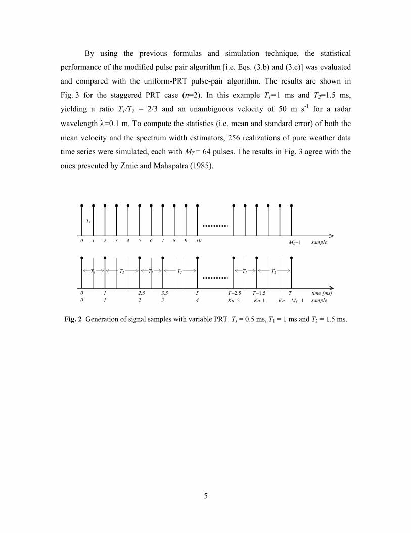
The simulation of signal samples like the ones shown in Fig. 1 can be

accomplished by using MS uniformly sampled points and then “dropping” the unwanted

samples to get the specified PRT scheme. Figure 2 illustrates this process for the simple

case of T1=1 ms and T2=1.5 ms. Here we used a uniform sampling frequency (1/Ts) of

2 kHz and kept only the samples 0, 2, 5, 7, 10, 12, 15, ...

T1

sample

R(1)(T1)

0 1 2 n−1

T2

R(1)(T2)

Tn

n

T1

n+1 Kn−1

Tn

Kn= MT −1

T2

n+2

R(2)(T2) R(2)(T1) R(1)(Tn) R(K)(Tn)

Basic PRT sequence

5

By using the previous formulas and simulation technique, the statistical

performance of the modified pulse pair algorithm [i.e. Eqs. (3.b) and (3.c)] was evaluated

and compared with the uniform-PRT pulse-pair algorithm. The results are shown in

Fig. 3 for the staggered PRT case (n=2). In this example T1=1 ms and T2=1.5 ms,

yielding a ratio T1/T2 = 2/3 and an unambiguous velocity of 50 m s-1 for a radar

wavelength λ=0.1 m. To compute the statistics (i.e. mean and standard error) of both the

mean velocity and the spectrum width estimators, 256 realizations of pure weather data

time series were simulated, each with MT = 64 pulses. The results in Fig. 3 agree with the

ones presented by Zrnic and Mahapatra (1985).

Fig. 2 Generation of signal samples with variable PRT. Ts = 0.5 ms, T1 = 1 ms and T2 = 1.5 ms.

sample 0 MS −1 1 2 3 4 5 6 7 8 9 10

Ts

T1

time [ms] 0 1 2.5 3.5

T2

5 Kn−1 Kn = MT −1

T1 T2 T1 T2

0 1 2 3 4 T

Kn−2T –1.5T –2.5

sample

6

0 2 4 6 8−1

−0.5

0

0.5

1

Spectrum Width, σv (m s−1)

Bia

s{v}

(m

s−

1 )

0 2 4 6 8−0.5

0

0.5

1

1.5

2

2.5


Bia

s{σ v}

(m s

−1 )

0 2 4 6 80

0.5

1

1.5

2

2.5

3

3.5

4


Std{

σ v} (m

s−

1 )

256 realizations M

t = 64

SNR = 20 dB T

1 = 1.00 ms

T2 = 1.50 ms

λ = 10 cm v

a = 50 m s−1

0 2 4 6 80

1

2

3

4

5


Std{

v} (

m s

−1 )

Uniform PRT − TStaggered PRT − 2T,3T

Fig. 3 Statistical performance of the pulse pair algorithm. Staggered PRT with T1=1 ms, T2=1.5 ms and MT = 64 pulses. Uniform PRT with Ts=T2−T1 for same unambiguous velocity and MS = 160 pulses for same dwell time. For both schemes 256 realizations of time series data were

simulated with λ=10 cm and SNR=20 dB.

4. Ground Clutter Filter

As stated previously, ground clutter filters (GCF) are high-pass filters that ideally

remove a few frequency components at either side of the zero Doppler velocity and leave

the rest of the spectrum almost intact. It is very important to comply with this property

during the design phase, because any changes in the magnitude response will directly bias

the estimates of the three parameters of interest. On the other hand, it is relatively easy to

prove that the phase characteristic of the filter is immaterial. To observe this, recall that

power, mean velocity and spectrum width estimates depend on the estimated

autocorrelation function of the filtered weather signal. It is well known that the power

spectral density (psd) of the output of a linear time-invariant filter Sy(ω) is related to the

7

psd of the input Sx(ω) by the magnitude square of the frequency response of the filter.

That is

2)()()( ωω=ω HSS xy . (5)

Moreover, the autocorrelation function is uniquely determined by the corresponding psd

through a Fourier transform pair relation. Because the phase response of the filter is not

involved in this transformations it has no effect on the autocorrelation.

Unfortunately, this analysis does not apply when sampling is non-uniform. The

linear time-invariant filter theory becomes useless when dealing with input samples

arriving at different rates. Intrinsically, the non-uniform sampling process introduces a

new series of complications in the analysis and design of suitable filters for clutter

suppression. Nevertheless, a few approaches have been studied for clutter rejection filters

operating with samples at non-uniform rates.

Banjanin and Zrnic (1991) used a time-varying filter that alternates between two

sets of coefficients, one for each of the staggered PRTs. Their filter was affected by the

staggering process in such a way that distortions in magnitude and phase occurred at

frequencies given by integer multiples of 1/(T1+T2). A complicated, yet questionable

scheme was proposed to mitigate the deleterious effects at these frequencies. On the other

hand, Chornoboy (1994) proposed a multiple PRT scheme where the effects of non-

uniform spacing would be spread uniformly over the unambiguous velocity interval. This

might lead to tolerable degradation of velocity estimates everywhere. However, no

comprehensive simulations or analysis of Chornoboy’s filter are available.

Here we investigate the suitability of regression filters for ground clutter

elimination and compare performance to the 5th-order elliptic infinite-impulse-response

(IIR) ground clutter filter (GCF) implemented in the WSR-88D. Application of

regression filters to clutter suppression in Doppler ultrasonic blood flow meters was

presented by Hoeks et al (1991) and extended by Kadi et al (1995) and Torp (1997) in

the context of uniform PRT. Application of first order regression GCF to wind profiling

radars is demonstrated by May and Strauch (1998). As a further step, we attempt to

8

extend practical application of regression filters to Doppler weather radars that use

variable PRTs, and analyze some of the inherent problems discussed above.

4.1. Orthogonal Polynomials

The essential element of a regression filter is the operation that projects the input

signal into what we identify as the “clutter signal subspace.” This projection block

performs the approximation of the input signal using a linear combination of the

functions in the basis representing the subspace of interest. Consequently, the filter

designer faces the issue of defining the functions in the basis of such subspace according

to the filter performance specifications.

Projections of elements from a vector space S (the signal vector space) into a

subspace W of S (the clutter signal space) can be efficiently performed when this

subspace is represented by an orthogonal basis B. However, orthogonality alone is not

sufficient to completely specify this basis. To improve the computational efficiency of

this filtering process, we can limit the functions in B to polynomials over a set of discrete

points on the real line. Therefore, for the general case, B will be a set of discrete

orthonormal polynomials over a non-uniformly spaced set of sampling times.

Orthogonal polynomials have received a lot of attention in applications such as

rational interpolation, least squares polynomial approximation, and smoothing of non-

linear functions. Egecioglu and Koc (1992) presented an efficient algorithm to generate

this set of polynomials over an arbitrary set of points },,,{}{ 110 −=TMm tttt . In their work

they consider the generation of a basis )}(,),(),({ 10 tbtbtbB p…= 1 where for every ji ≠ ,

pji ≤≤ ,0

( ) 0)()()(),(1

0

== ∑−

=

TM

mmjmiji tbtbtbtb . (6)

1 t is included to explicitly show that each element of B is a function of time

9

This set of orthogonal polynomials can be generated using the classical three-term

recursion formula

)()()()( 11 miimiimmi tbtbttb −+ β−α−= for 0 < i < p and 0 < m < MT −1, (7)

with 0)(1 =− mtb and 1)(0 =mtb , and where αi and βi are constants determined as

( )( ))(),(

)(),(tbtbtbttb

ii

iii =α , ( )

( ))(),()(),(

11 tbtbtbtb

ii

iii

−−

=β . (8)

For p=5 the set of orthogonal polynomials is depicted in Figure 4 over a sample

set given by {tm}={0, 2, 5, 7, 10, 12, 15, ... , 77}, i.e. MT =32 with staggered PRT and

underlying time set corresponding to T1/T2=2/3.

0 10 20 30 40 50 60 70 80−0.4

−0.3

−0.2

−0.1

0

0.1

0.2

0.3

0.4

time (tm

)

b i(tm

)

Orthogonal polynomial set − p=5 − Variable PRT scheme

// / /

/

b0

b1

b2

b3 b

4b

5/

Fig. 4 Orthogonal polynomials on a non-uniformly spaced time grid with T1/T2=2/3.

4.2. Regression Filters

Classical digital filters can be divided into two classes: finite impulse response

(FIR) and infinite impulse response (IIR) filters. For either class, filtering is achieved by

10

superposition of signal samples. Unlike these filters, regression filters approximate their

input signals with polynomial functions in the time domain, and their design is not based

on traditional tools such as the impulse or frequency responses. In our case, it can be

assumed that the clutter signal varies slowly compared to the weather echo signal, and

consequently can be approximated by a polynomial of a relatively low degree. This

approximation is usually performed using least-squares methods or the equivalent

transformation which projects the input signal samples V(t), }{ mtt ∈ onto the subspace W

spanned by a basis B consisting of p+1 orthonormal polynomials. This set of polynomials

is given by B={b0(t),b1(t),b2(t),...,bp(t)}, where each bi(t) (0 < i < p) is a polynomial of

ith degree. That is, iiiiii tctcctb +++= ...)( 10 with }{ mtt ∈ . Then, the projection )(ˆ tV (i.e.

the clutter signal) is obtained by constructing a linear combination of the elements of the

basis B, i.e. implication is that )(ˆ tV is in W and therefore

∑=

α=p

imiim tbtV

0

)()(ˆ . (9)

Accordingly, the residue )(ˆ)()( mmmf tVtVtV −= is associated with the portion of

the input signal that is not contained in the clutter subspace W [i.e. it is orthogonal to

)(ˆ tV ]. The coefficients αi ‘s are computed using the classical formula (Papoulis 1986,

146-154)

( )

∑

∑−

=

−

===α 1

0

2

1

02

)(

)()(,

f

f

M

mmi

M

mmim

i

tb

tbtV

i

i

bbV i = 0, 1, ..., p. (10)

Generalization in this analysis is not lost if each element of B is normalized such

that 1=ib , where ( )iii bbb ,2 = . In addition, to simplify the notation define the basis

matrix B and the coefficient vector A as

11

=

−

−

−

)()()(

)()()()()()(

110

111101

101000

f

f

f

Mppp

M

M

tbtbtb

tbtbtbtbtbtb

B and

α

αα

=

p

1

0

Α . (11)

Then, assuming a normalized base, Eqs. (9) and (10) can be rewritten as

ABV T=ˆ . Substitution of BVΑ = produces BVBV T=ˆ and the residue or filtered signal

Vf can be expressed as

VBBIVVV Tf )(ˆ −=−= , (12)

where the regression filter matrix is defined by

BBIF T−= . (13)

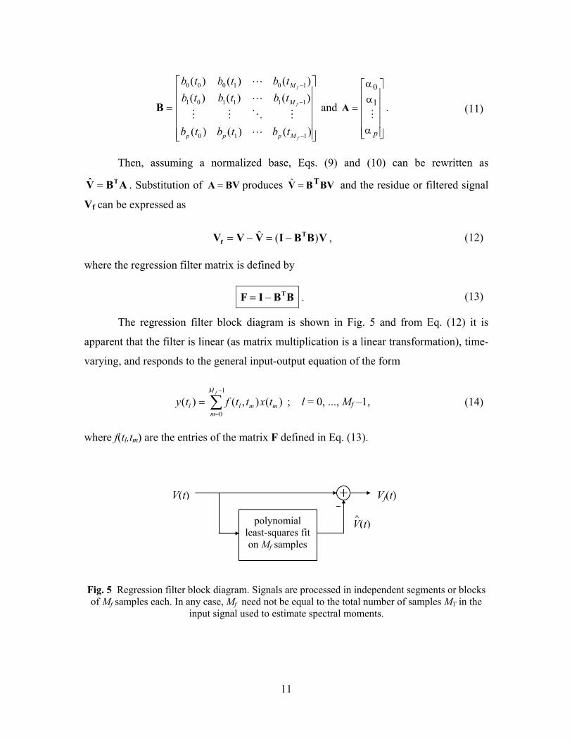
The regression filter block diagram is shown in Fig. 5 and from Eq. (12) it is

apparent that the filter is linear (as matrix multiplication is a linear transformation), time-

varying, and responds to the general input-output equation of the form

∑−

=

=1

0

)(),()(fM

mmmll txttfty ; l = 0, ..., Mf –1, (14)

where f(tl,tm) are the entries of the matrix F defined in Eq. (13).

Fig. 5 Regression filter block diagram. Signals are processed in independent segments or blocks of Mf samples each. In any case, Mf need not be equal to the total number of samples MT in the

input signal used to estimate spectral moments.

polynomial least-squares fit on Mf samples

V(t) Vf(t)

V(t)^

12

The filter matrix F depends only on p and Mf, so it can be pre-computed for real-

time applications and does not need to be recomputed if the notch width or sampling

scheme do not change. In any case, Mf need not be equal to the total number of samples

MT in the input signal used to estimate spectral moments.

Several approaches can be devised if MT >Mf, according to the way the input

signal is decomposed into the samples blocks to be least squares fitted. For our study, we

adopted overlapping blocks, attempting to simulate the behavior of a moving average

filter. In this implementation, special care must be taken on both ends of the input

sequence. The scheme can be summarized as follows: the first Mf/2 output samples are

computed as in Eq (14). From sample Mf/2 +1 and up to sample MT – Mf/2 the output is

computed by sliding the (Mf/2 +1)-th column of F, i.e. tl inside the summation in Eq(14)

is fixed to Mf/2+1. Finally, the last Mf/2 output samples are computed as in Eq (14). Note

that if MT = Mf, the process reduces to Eq. (14).

4.3. Frequency Response of the Regression Filter

The frequency response H(ω) of a linear shift-invariant system can be defined as

the change in magnitude and phase of a complex exponential signal ejωt which is passed

through the system. More precisely, let x(t) and y(t) be the input and output of the filter

whose impulse response is given by h(t). Let tjetx 0)( ω= , then the output y(t) can be

obtained by convolving x(t) with h(t), i.e.

, )()( )'(

)'()'()'()(*)()(

0}{'

'

}{'

)'(

}{'

00

0

txHeeth

ethttxthtxthty

tj

tt

tj

tt

ttj

tt

m

mm

ω=

=

==−==

ω

∈

ω−

∈

−ω

∈

∑

∑∑ (15)

in which H(ω0) describes the frequency response at ω = ω0.

As previously stated, the regression filter is time varying. However, the output to

a given signal of Mf samples is always the same regardless when this block of Mf samples

is encountered in the filtering process. We will exploit this fact in deriving an expression

13

for the frequency response of the regression filter using Eq. (14) in an analogous fashion

as Eq. (15). That is, consider the regression filter whose input is an exponential of the

form ejωt. The output of this filter is

∑−

=

ω=1

0

),()(f

m

M

m

tjmll ettfty ; l = 1, ..., Mf (16)

)( ),(),()(1

0

1

0

)(l

tjM

m

tjml

M

m

tjttjmll txeettfeettfty l

f

m

f

llm ω−−

=

ω−

=

ω−ω

== ∑∑ . (17)

Then, by noting the form of (17) we define

ltjll eFtH ω−ω−=ω )(),( , (18)

where ∑−

=

ω−=ω1

0

),()(f

m

M

m

tjmll ettfF is the DFT of f(tl,tm) with constant parameter l. Finally,

accounting for all the values of l in the Mf -sample segment

∑−

=

ω−ω−=ω1

0

1 )()(f

l

f

M

l

tjlM eFH . (19)

Using the results of Eq. (13), each entry in F is given by

∑=

−−δ=p

imilimlml tbtbttttf

0

)()()(),( , (20)

where δ(t) is the usual discrete-time impulse sequence. Then

∑=

ω− ω−=ωp

iili

tjl BtbeF l

0

)()()( , (21)

where Bi(ω) is the DFT of bi(t). Then,

∑ ∑=

−

=

ω−

ω−−=ω

p

i

M

l

tjliiM

f

l

fetbBH

0

1

0

1 )()(1)( , (22)

and finally the frequency response of the regression filter is given by

14

∑=

ω−=ωp

iiM BH

f0

21 )(1)( . (23)

Note that because H(ω) is real, the phase response of this filter is constant and we

only need to consider the changes in the magnitude response. Also, as depicted in Fig. 5,

H(ω) consists of a direct path, the “1” in Eq. (23), and a weighted path given by the least

squares fit projection and corresponding to the second term in the same equation.

The frequency response of the regression filter depends on the number p of

elements in B (i.e. the maximum degree of the polynomials used for approximation) and

on the number of samples Mf in each processing block. High-frequency signals exhibit

rapid changes in time and hence, they are better approximated as p increases. Therefore,

by increasing p, we allow high-frequency components to be subtracted from the input

signal, and this results in a broader notch width. On the other hand, for a fixed p higher

frequencies are eliminated if the filter window Mf is shorter. That is, polynomials of a

relatively low degree can still “follow” high-frequency components. Consequently, the

notch width of the regression filter increases when Mf decreases. This dependence is

illustrated in Fig. 6 for the uniform PRT scheme. From these plots, we can confirm that

the notch bandwidth increases with p and decreases as Mf increases. Observe that in

Fig. 6.c MT = 2Mf and the filtering scheme discussed in the previous section is

implemented. Frequency responses for the regression filter change just slightly with

respect to Fig. 6.b.

The WSR-88D 5th-order elliptic GCF can be programmed for three different

suppression levels: low suppression, medium suppression, or high suppression. These

selections correspond to notch widths of 2.36 m s-1 (±1.18 m s-1), 3.12 m s-1 (±1.56 m s-1),

and 5.06 m s-1 (±2.53 m s-1), which do not change with the number of samples MT. The

steady-state frequency responses of the low, medium and high suppression 5th-order

elliptic GCF for the WSR-88D are also plotted for comparison. The general form of the

transfer function of this filter is

15

55

44

33

22

11

55

44

33

22

110

1)(88 −−−−−

−−−−−

−−−−−+++++

=− zazazazazazbzbzbzbzbbzH DWSR , (24)

where the coefficients ai’s and bi’s are obtained from the classical design formulas for

digital elliptic filters as given in Parks and Burrus (1987).

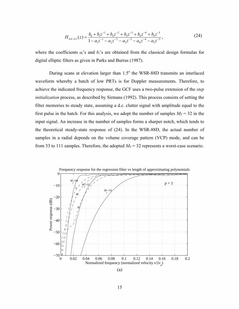
During scans at elevation larger than 1.5o the WSR-88D transmits an interlaced

waveform whereby a batch of low PRTs is for Doppler measurements. Therefore, to

achieve the indicated frequency response, the GCF uses a two-pulse extension of the step

initialization process, as described by Sirmans (1992). This process consists of setting the

filter memories to steady state, assuming a d.c. clutter signal with amplitude equal to the

first pulse in the batch. For this analysis, we adopt the number of samples MT = 32 in the

input signal. An increase in the number of samples forms a sharper notch, which tends to

the theoretical steady-state response of (24). In the WSR-88D, the actual number of

samples in a radial depends on the volume coverage pattern (VCP) mode, and can be

from 33 to 111 samples. Therefore, the adopted MT = 32 represents a worst-case scenario.

0 0.02 0.04 0.06 0.08 0.1 0.12 0.14 0.16 0.18 0.2−70

−60

−50

−40

−30

−20

−10

0

Normalized frequency (normalized velocity v/2va)

Pow

er r

espo

nse

(dB

)

Frequency response for the regression filter vs length of approximating polynomials

Mf=64

Mf=32

Mf=16

p = 3L

M

H

(a)

16

0 0.02 0.04 0.06 0.08 0.1 0.12 0.14 0.16 0.18 0.2

−70

−60

−50

−40

−30

−20

−10

0


Pow

er R

espo

nse

(dB

)

Frequency response for the regression filter vs. maximum order of approximating polynomials

p=1

p=2

p=3

MT = M

f = 32

L

M

H

(b)

0 0.02 0.04 0.06 0.08 0.1 0.12 0.14 0.16 0.18 0.2−70

−60

−50

−40

−30

−20

−10

0


Pow

er R

esponse

(dB

)

Frequency response for the regression filter vs. maximum order of approximating polynomials

L

M

p=3 p=2

p=1

H

MT = 64 M

f = 32

(c)

Fig. 6 Regression filter frequency response with p and Mf as parameters. The frequency responses of the low (L), medium (M) and high (H) suppression 5th-order elliptic filter used in the

WSR-88D are also included for comparison. The two-pulse extension of the step initialization process is used to improve the response, i.e. suppress the transient due to the step inputs at the

beginning of pulse bursts for velocity estimation.

17

Figure 7 shows how the filter’s 3 dB notch width depends on the number of

samples, for both classes of GCFs. As a useful tool for further comparison, we find a

direct equivalence between each suppression level of the 5th-order elliptic filter and the

order of approximating polynomials in the regression filter. We observe, for instance, that

for p = 3 and Mf = 32, the notch width of the regression filter closely matches that of the

medium suppression GCF in the WSR-88D.

The regression filter has several attractive properties compared to the GCF

currently implemented in the WSR-88D. While the latter is greatly influenced by the

filter’s transient response characteristics, the regression filter inherently avoids these

transients (i.e. these filters do not cause transients). Moreover, regression filters design

methods diverge from the ones used with classical filters, because their implementation

consists of a matrix multiplication instead of a set of equations to evaluate recursively for

each time. Thus, the regression filter is well suited for modern array processors.

25 30 35 40 45 50 55 60 65 70 750

0.01

0.02

0.03

0.04

0.05

0.06

0.07

Number of samples − Mf

Nor

mal

ized

NW

− n

w/2

v a

Regression filter notch width vs. Mf

p = 2

p = 3

p = 4Low Supp.

Medium Supp.

High Supp.

Fig. 7 Regression filter notch width vs. number of uniformly spaced samples and order of approximating polynomials.

18

5. Performance Analysis of the Regression Filter

5.1. Uniform PRT Scheme

In this section, we carry simulations to establish the performance of the regression

filter and compare it with the 5th-order elliptic GCF implemented in the WSR-88D. The

clutter signal is modeled as a narrow-band Gaussian process with zero mean velocity.

This clutter and white noise are added to a synthetic weather signal (Zrnic 1975). Then,

the composite signal is filtered to remove the ground clutter and finally the first three

moments of the weather Doppler spectrum are estimated with the classical pulse pair

algorithm. This process is shown in Fig. 8.

−30 −20 −10 0 10 20 30

10

20

30

40

50

60

70

80

90

100

v [m s−1]

|V(f

)| −

line

ar s

cale

Clutter

Weathersignal

CSR = 10dBsignal

(a) 0 10 20 30 40 50 60

−2

−1.5

−1

−0.5

0

0.5

1

1.5

2

time

Re{

V(f

)}

Input Signal

(b)

−30 −20 −10 0 10 20 30

0

10

20

30

40

50

60

70

80

90

100

v [m s−1]

|Vf(f

)| −

line

ar s

cale

Filteredsignal

(d) 0 10 20 30 40 50 60

−2

−1.5

−1

−0.5

0

0.5

1

1.5

2

2.5

time

Re{

Vf(f

)}

Output Signal

(c)

Fig. 8 Clutter filtering process using a regression filter. (a) Spectrum of a weather signal contaminated with ground clutter. (b) Time-domain representation of the composite signal. The dashed line is the 3rd-order polynomial fit to this signal, i.e., the estimated clutter. (c) Filtered

signal in the time domain used to determine S, v and σv from Eq. (3). (d) Spectrum of the filtered signal.

Regression Filter

19

Two parameters of interest for these simulations are: the signal-to-noise ratio

(SNR) and the clutter-to-signal ratio (CSR) which are defined as

( )NSdBSNR /log10)( 10= and ( )SCdBCSR /log10)( 10= where S, C and N are signal,

clutter and noise powers respectively. The clutter filter suppression ratio (CFSR), a

measure of the filter’s performance, is defined by )/(log10)( 10 inout PPdBCFSR = . In this

equation Pin and Pout are the powers measured at the input and output of the clutter filter

respectively (note that Pin = C+S+N and ideally Pout = S+N). Figure 9 shows the CFSR if

no weather signal is present at the input of the filter with the clutter spectrum width as a

parameter. The behavior of both the regression filter and the WSR-88D elliptic filter

described in Section 4 is depicted in the same figure. It is observed that for the most

common case of narrow clutter spectrum widths, i.e. σc < 0.5 m s-1, the suppression ratio

of the regression filter with p = 4 is at least 10 dB better than the one achieved by the

high-suppression elliptic GCF. In general, the regression filter performs better than the

comparable elliptic filter, especially if the spectrum width of the clutter is narrow.

0 0.2 0.4 0.6 0.8 1−120

−100

−80

−60

−40

−20

0

Clutter spectrum width, σc [m s−1]

Supr

essi

on R

atio

: 10l

og10

(Pou

t/Pin

)

Ground clutter filter suppression ratio (S = N = 0)

Regression filter. p=2Regression filter. p=3Regression filter. p=4WSR−88D low suppWSR−88D medium suppWSR−88D high supp

MT = 32

Mf = 32

va = 25m s−1

Fig. 9 Suppression ratio vs. clutter signal spectrum width when no weather signal is present.

20

0 5 10 15 20 25−4

−3.5

−3

−2.5

−2

−1.5

−1

−0.5

0

0.5

Weather signal mean velocity, v [m s−1]

Supr

essi

on R

atio

: 10l

og10

(Pou

t/Pin

)

Ground clutter filter suppression ratio (C = N = 0)


MT = 32

Mf = 32

σv = 4m s−1

va = 25m s−1

(a)

0 5 10 15 20 25−20

−15

−10

−5

0

5


Supr

essi

on R

atio

: 10l

og10

(Pou

t/Pin

)



MT = 32

Mf = 32

σv = 1m s−1

va = 25m s−1

(b)

Fig. 10 Suppression ratio vs. signal spectrum mean velocity when no clutter signal is present. (a) σv = 4 m s-1 (median value in severe storms) ; (b) σv = 1 m s-1 (typical value in stratiform rain)

21

The suppression of weather-like signals by these filters is plotted in Fig. 10,

where the mean velocity changes from 0 to 25 m s-1, and the spectrum width is set

constant. A value of 4 m s-1 in Fig. 10.a simulates the median found in severe storm

observations (Doviak and Zrnic, 1993). Over 1 dB of suppression is observed for signal

mean velocities below 5 to 8 m s-1, depending on the notch width of the filter. At that,

performances of regression filters are comparable to the elliptic filters of corresponding

notch width. Similar results hold for weather signals with spectrum width of 1 m s-1

(typical of stratiform rain) except the 1 dB suppression is for velocities below 3.5 to

4.5 m s-1 (Fig. 10.b). These curves indicate the power estimation biases one can expect if

the mean velocity of the weather signal is close to zero. However, when the mean

velocity of the weather signal is well away from 0 m s-1, neither of the filters biases the

power estimates.

For a more realistic situation, a weather signal was combined with the ground

clutter and the ratio Pout/S was computed for different CSRs. This analysis is shown in

Figs. 11.a and 11.b for a CSR of 20 and 40 dB respectively. The clutter spectrum width is

set at 0.28 m s-1 for the first case (Fig 11.a) and 0.23 m s-1 for the second case (Fig. 11.b).

The first value is the same as the one used for testing the WSR-88D ground clutter filter

performance (Sirmans, 1992). Measurements on the WSR-88D in Norman, OK indicate

that the mean of clutter spectrum width is 0.25 m s-1; therefore, 0.28 m s-1 is in the worst

case category. However, this value is too large if the CSR equals 40 dB causing excessive

contamination, and a smaller value of 0.23 m s-1 is adopted in Fig. 11.b. It is seen in

Fig. 11 that the reflectivity estimates can have a significant negative bias if the mean

Doppler velocity of the weather signal is such that its spectrum overlaps the one of the

ground clutter. This is because the ground clutter filter also removes a portion of the

weather signal. In addition, we observe a small positive bias (WSR-88D low suppression)

if the mean Doppler velocity departs from the origin for a CSR of 20dB, because the

clutter signal is not fully removed by the filter. For the CSR of 40dB, we found that the

elliptic GCF does not remove the clutter signal completely leaving an almost constant

bias along the entire velocity range. The same occurs with the 2nd-order regression filter

but the 3rd- and 4th-order regression filters had no bias. Evidently, this effect gets worse

22

for larger CSR and wider clutter spectrum width but it can be controlled by adjusting the

ground clutter filter frequency response.

0 5 10 15 20 25−4

−3.5

−3

−2.5

−2

−1.5

−1

−0.5

0

0.5

1


10lo

g 10(P

out/S

)

Ground clutter filter suppression preformance


CSR = 20dB SNR = ∞ M

T = 32

Mf = 32

σv = 4m s−1

σc = 0.28m s−1

va = 25m s−1

(a)

0 5 10 15 20 25−5

0

5

10

15


10lo

g 10(P

out/S

)

Ground clutter filter suppression preformance


CSR = 40dB SNR = ∞ M

T = 32

Mf = 32

σv = 4m s−1

σc = 0.23m s−1

va = 25m s−1

(b)

Fig. 11 Supp. ratio of regression and elliptic GCFs vs. weather signal mean velocity.

(a)CSR=20dB, (b)CSR=40dB

23

As the ultimate goal is to accurately recover the three first spectral moments of

the weather signal, the pulse pair statistical performance for different CSRs was

computed vs. (a) the weather signal mean velocity and (b) the weather signal spectrum

width for both regression and elliptic WSR-88D filters. The results are shown in Fig. 12.

Consider first the case when the weather signal mean velocity is a parameter and

the spectrum width is randomly selected from the interval (2,6) m s-1 (Figs. 12.a and

12.b). Here we observe that there are large positive biases for both the mean velocity and

the spectrum width estimates when the true mean velocity of the weather signal is less

than approximately 5 m s-1. As explained before, this is due to overlap of the weather and

clutter spectra. A part of this spectrum close to zero velocity is eliminated by the filter;

therefore, the non-filtered components bias the velocity upward. Mean velocity bias for

the regression filter is about 0.25 m s-1 larger than for the elliptic filter at v < 10 m s-1.

The standard deviation for the velocity estimation remains under 2 m s-1 and very close to

the performance of the pulse-pair algorithm in the absence of clutter. Keeping a high SNR

and increasing the CSR, from Fig. 12.a to Fig. 12.b, does not significantly affect the

statistical performance of the pulse pair algorithm. When increasing the order of the

regression filter, from p=3 to p=4 (not shown), we do observe an increase in the biases

for weather signals with mean velocities near 0 m s-1 which is caused by the broader

notch width of this filter.

Next, we use the weather-signal spectrum width as a parameter and randomly

select its mean velocity from the interval (-25,25) m s-1 (Figs. 12.c and 12.d). In this case,

we notice that the variation in mean velocity bias and standard deviation increase with the

weather signal spectrum width. This effect is consistent with the autocovariance

algorithm performance; it is and slightly more evident if there is contamination by the

clutter signal. The bias in v and the standard deviations for the two filters are comparable.

A slightly smaller bias and standard deviation are seen in spectrum width estimates.

Because the GCF does not remove the clutter signal completely, for small spectrum

widths, we observe a positive bias in the spectrum width estimates, which increases with

the CSR. From all these figures, we conclude that influences of the regression filter and

24

0 5 10 15 20 25−0.5

0

0.5

1

1.5

2

Mean Velocity, v (m s−1)

Bia

s{v}

(m

s−

1 )

0 5 10 15 20 25−0.5

0

0.5

1

1.5

2


Bia

s{σ v}

(m s

−1 )

0 5 10 15 20 250.5

0.75

1

1.25

1.5


Std{

σ v} (m

s−

1 )

256 realizations M

T = 32

Mf = 32

SNR = ∞ CSR = 20 dB σ

c = 0.28 m s−1

λ = 10 cm v

a = 25 m s−1

0 5 10 15 20 250.8

1

1.2

1.4

1.6

1.8

2


Std{

v} (

m s

−1 )

Unif − No ClutUnif − Reg filt − p=3Unif − WSR−88D GCF (M)

(a)

0 5 10 15 20 25−0.5

0

0.5

1

1.5

2


Bia

s{v}

(m

s−

1 )

0 5 10 15 20 25−0.5

0

0.5

1

1.5

2


Bia

s{σ v}

(m s

−1 )

0 5 10 15 20 250.5

0.75

1

1.25

1.5


Std{

σ v} (m

s−

1 )

256 realizations M

T = 32

Mf = 32


c = 0.23 m s−1

λ = 10 cm v

a = 25 m s−1

0 5 10 15 20 250.8

1

1.2

1.4

1.6

1.8

2


Std{

v} (

m s

−1 )


(b)

25

0 1 2 3 4−0.4

−0.2

0

0.2

0.4

0.6

0.8

1


Bia

s{v}

(m

s−

1 )

0 1 2 3 4−0.5

0

0.5

1

1.5

2

2.5


Bia

s{σ v}

(m s

−1 )

0 1 2 3 40

0.2

0.4

0.6

0.8

1

1.2

1.4

1.6

1.8

2


Std{

σ v} (m

s−

1 )

256 realizations M

T = 32

Mf = 32


c = 0.28 m s−1

λ = 10 cm v

a = 25 m s−1

0 1 2 3 40

0.2

0.4

0.6

0.8

1

1.2

1.4

1.6

1.8

2


Std{

v} (

m s

−1 )


(c)

0 1 2 3 4−0.4

−0.2

0

0.2

0.4

0.6

0.8

1


Bia

s{v}

(m

s−

1 )

0 1 2 3 4−0.5

0

0.5

1

1.5

2

2.5


Bia

s{σ v}

(m s

−1 )

0 1 2 3 40

0.2

0.4

0.6

0.8

1

1.2

1.4

1.6

1.8

2


Std{

σ v} (m

s−

1 )

256 realizations M

T = 32

Mf = 32


c = 0.23 m s−1

λ = 10 cm v

a = 25 m s−1

0 1 2 3 40

0.5

1

1.5

2

2.5

3


Std{

v} (

m s

−1 )


(d)

Fig. 12 Pulse pair algorithm statistical performance. (a),(b) vs. the weather signal mean velocity; (c),(d) vs. the weather signal spectrum width. For all simulations we used a medium-suppression

filter (p = 3), 256 realizations, and an unambiguous velocity of 25 m s-1.

26

the corresponding elliptic filter on the statistical performance of pulse pair estimators are

comparable.

5.2. Application of filters to the WSR-88D data

Time series data have been collected with a WSR-88D in Memphis at the lowest

elevation of 0.5° while the antenna was scanning at 12° s-1. Sixty-four samples of the in-

phase component (Fig. 13.a) reveal a slowly varying clutter signal and possibly weak

weather signal. The Doppler spectrum (Fig. 13.b) has a peak at zero, which is 75 dB

above the receiver noise level. This large spectral dynamic range has been routinely

observed on both Memphis and Norman WSR-88D and testifies to the very high quality

of the system. The spectrum width of this ground clutter is 0.23 m s-1, the CSR is 33 dB

and the SNR is 26 dB.

Application of the regression filter with p=3 produces signals in Fig. 14 whereas

the medium suppression elliptic filter provides the signals in Figs. 15 and 16. The

regression filter with Mf =32 is applied to the 64 input samples similarly to a moving

average filter as explained in Section 4.2. Note how the in-phase signal after regression

filtering has no discernible slow varying component whereas after filtering with the

elliptic filter it does. This is also reflected in the spectral shapes at and close to zero

velocity. The clutter spectrum has been suppressed at least 40 dB below the weather peak

after application of the regression filter (Fig. 14.b) and it is slightly below the weather

peak after application of the elliptic filter (Fig. 15.b). For the non-initialized elliptic filter

in Fig. 16, the results are inferior, as evidenced by the higher residual clutter power with

spectral peaks slightly above the weather signal peak level. This demonstrates the

advantage of step initialization in the WSR-88D.

27

0 10 20 30 40 50 60

0.8

1

1.2

1.4

1.6

1.8

time (ms)

I =

Re{

V}

Original time series data

−25 −20 −15 −10 −5 0 5 10 15 20 25

−80

−60

−40

−20

0

20

Doppler velocity − v (m s−1)

10*l

og 1

0(|S|2 )

(dB

)

Fig. 13 Data collected with the WSR-88D in Memphis at a range of 15 km. (a) In-phase component and (b) Doppler spectrum of the time series to which the von Hann window has been

applied.

0 10 20 30 40 50 60

−0.05

0

0.05

0.1

time (ms)

I =

Re{

V}

Filtered time series data − Regression filter (p=3)

−25 −20 −15 −10 −5 0 5 10 15 20 25

−80

−60

−40

−20

0


10*l

og 1

0(|S|2 )

(dB

)

Fig. 14 Time series data filtered with the “medium suppression” regression filter (p=3). (a) In-phase filtered component and (b) Doppler spectrum of the filtered signal (weighted with the von

Hann window).

28

0 10 20 30 40 50 60

−0.1

−0.05

0

0.05

time (ms)

I =

Re{

V}

Filtered time series data − WSR−88D elliptic filter (Med supp)

−25 −20 −15 −10 −5 0 5 10 15 20 25

−80

−60

−40

−20

0


10*l

og 1

0(|S|2 )

(dB

)

Fig. 15 Same as in Fig. 14 except the medium suppression WSR-88D ground clutter filter has been applied.

0 10 20 30 40 50 60−0.5

0

0.5

time (ms)

I =

Re{

V}

Filtered time series data − WSR−88D elliptic filter (Med supp) − No initialization

−25 −20 −15 −10 −5 0 5 10 15 20 25

−80

−60

−40

−20

0


10*l

og 1

0(|S|2 )

(dB

)

Fig. 16 Same as in Fig. 15 except the 5th-order elliptic ground clutter filter has not been initialized according the the two-pulse extension of the step initialization, as implemented in the

WSR-88D.

29

5.3. Staggered PRT Scheme

As pointed out in the introduction, the motivation for this analysis is the need for

an effective method to suppress ground clutter in variable PRT sequences used to

mitigate the effects of range-velocity ambiguities. The regression filter appears to be a

promising approach to solve this problem because it can be readily generalized to the

non-uniform PRT scheme (as it does not require using frequency-domain design

techniques). Moreover, the necessary tools exist for generating a set of orthogonal

polynomials over a non-uniform sampling grid and consequently it is feasible to

implement a ground clutter filter in the context of variable PRT. However, as

demonstrated by simulations, the regression filter does not avoid the previously

encountered problems (Banjanin and Zrnic, 1991). This filter also exhibits additional

notches at the normalized frequencies given by f = nTS/(T1+T2), where Zn /∈ and TS is the

corresponding underlying uniform PRT from which the staggered PRT signal is derived.

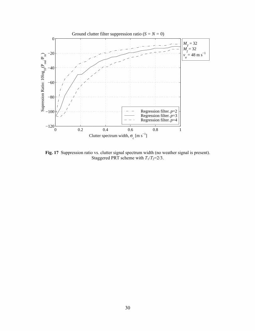
Throughout these simulations, we used the staggered PRT scheme with different

stagger ratios T1/T2. Figures 17 and 18 show the suppression ratio computed using the

parameters as in Figs. 9 and 10. From these plots, we observe that the clutter suppression

is comparable to the one achieved by the same filters on a uniform sequence of pulses.

However, this is not sufficient to accept the regression filter as a good candidate for

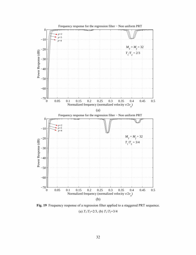
ground clutter canceling. The regression filter frequency response is deficient. Plots for

the two values of T1/T2 (Fig. 19) reveal the undesirable notches. The first plot (Fig 19.a)

corresponds to T1/T2=2/3 and clearly exhibits additional notches located at f = 0.2 n. The

second plot (Fig. 19.b) corresponds to T1/T2=3/4 and shows notches at f = 0.1429 n,

where as before Zn /∈ . As found by Banjanin and Zrnic (1991), these additional notches

introduce phase non-linearities which ultimately deteriorate the performance of the pulse

pair algorithm (because the algorithm is based on the phase of the autocorrelation of the

weather signal). This fact was verified by evaluating the statistical performance of the

autocovariance algorithm (Doviak and Zrnic, 1993, eq. 7.6a) on this particular PRT

scheme for T1/T2=2/3. The results are presented in Fig. 20 where we can see large bias

and standard deviation located exactly at the additional notch frequencies.

30

0 0.2 0.4 0.6 0.8 1−120

−100

−80

−60

−40

−20

0

Clutter spectrum width, σc [m s−1]

Supr

essi

on R

atio

: 10l

og10

(Pou

t/Pin

)

Ground clutter filter suppression ratio (S = N = 0)

Regression filter. p=2Regression filter. p=3Regression filter. p=4

MT = 32

Mf = 32

va = 48 m s−1

Fig. 17 Suppression ratio vs. clutter signal spectrum width (no weather signal is present). Staggered PRT scheme with T1/T2=2/3.

31

0 5 10 15 20 25−3

−2.5

−2

−1.5

−1

−0.5

0


Supr

essi

on R

atio

: 10l

og10

(Pou

t/Pin

)



MT = 32

Mf = 32

σv = 4m s−1

va = 48 m s−1

(a)

0 5 10 15 20 25−16

−14

−12

−10

−8

−6

−4

−2

0


Supr

essi

on R

atio

: 10l

og10

(Pou

t/Pin

)



MT = 32

Mf = 32

σv = 1m s−1

va = 48 m s−1

(b)

Fig. 18 Suppression ratio vs. weather signal mean velocity (no clutter signal is present). Staggered PRT scheme with T1/T2=2/3.

32

0 0.05 0.1 0.15 0.2 0.25 0.3 0.35 0.4 0.45 0.5−70

−60

−50

−40

−30

−20

−10

0


Pow

er R

espo

nse

(dB

)

Frequency response for the regression filter − Non uniform PRT

p=2

p=3

p=4

MT = M

f = 32

T1/T

2 = 2/3

(a)

0 0.05 0.1 0.15 0.2 0.25 0.3 0.35 0.4 0.45 0.5−70

−60

−50

−40

−30

−20

−10

0


Pow

er R

espo

nse

(dB

)

Frequency response for the regression filter − Non uniform PRT

p=2p=3 p=4

MT = M

f = 32

T1/T

2 = 3/4

(b) Fig. 19 Frequency response of a regression filter applied to a staggered PRT sequence.

(a) T1/T2=2/3, (b) T1/T2=3/4

33

0 10 20 30 40 50−15

−10

−5

0

5

10

15


Bia

s{v}

(m

s−

1 )

0 10 20 30 40 50−2

0

2

4

6

8


Bia

s{σ v}

(m s

−1 )

0 10 20 30 40 500

0.5

1

1.5

2

2.5

3


Std{

σ v} (m

s−

1 )

64 realizations M

S = 80

MT = 32

Mf = 32

SNR = 20 dB

CSR = −∞

λ = 10 cm v

a = 50 m s−1

0 10 20 30 40 500

5

10

15

20


Std{

v} (

m s

−1 )

Unif − No ClutUnif − Reg filt − p=3Stag − Reg filt − p=3 − k=2/3

Fig. 20 Statistical performance of the autocovariance algorithm applied to a staggered PRT sequence (T1/T2=2/3). The performances on (1) a uniform PRT sequence with no ground clutter and (2) a uniform PRT sequence and a 3rd-order regression filter are also included. The uniform and staggered PRT sequences were generated such that dwell times are the same for both. In the uniform PRT sequences MS =80, Ts=0.5 ms, and in the staggered PRT sequence MT =32, T1=2Ts, and T2=3Ts; therefore, both yield a maximum unambiguous velocity va of 50 m s-1. Large biases

and standard deviations appear at and near integer multiples of λ/[2(T1+T2)] (m s-1) when the regression filter is applied to the signal with staggered samples.

6. Future Work

There are still some variations to the variable PRT techniques and other aspects of

the design that deserve to be explored. These can be classified into the following

approaches:

Block PRT: where Ti is repeated mi consecutive times in an attempt to emulate the

uniform PRT scheme while keeping the advantages of having more than one PRT for

34

an extended velocity range. The regression filter (or any other GCF) can be applied

to each uniform batch independently.

Jittered PRT: where the periodicity of the sampling process is destroyed by using the

sequence { }mm TTTTTT δ+δ+δ+δ+ 21121121 ,,,,,, where δm<<T1,T2. With this

scheme, we expect the notches to be almost uniformly distributed along the entire

range of frequencies (Doppler velocities).

Almost Uniform PRT: where only one or two pulses with different PRT are added to

the uniform PRT scheme. It is possible to get good velocity estimates from the

uniform pulses, and then exploit information from pulses at different PRTs to correct

velocity aliases by shifting the estimates to the actual Nyquist interval (adding

integer multiples of 2va). This scheme was proposed by Cornelius et al (1993).

Extrapolation schemes as the one presented by Chornoboy (1993).

Implementation of Eqs. 3.b and 3.c with different autocorrelation ratios to obtain

better estimates of v and σv.

7. Conclusions

This initial report on regression filters tried to find the answer to two main

questions: (1) will a regression filter perform better than the current 5th-order elliptic filter

in the WSR-88D?, and (2) can this filter be applied to a non-uniform PRT sequence and

if so, what are the consequences on spectral moment estimates?

First, we compared the performance of the regression filter scheme applied to a

uniformly sampled sequence with that of the actual WSR-88D 5th-order elliptic filter. In

the context of uniform PRT, regression filters present the advantage of easy

implementation, not requiring filter initialization such as needed in the Doppler mode of

data processing at higher than 1.5o in elevation on the WSR-88D. Parameters that control

the frequency response are the number of samples to which regression is applied and the

degree of the regression polynomial. The increase in the polynomial degree (p) broadens

35

the filter's notch width because higher frequencies are subtracted from the signal. The

notch width also broadens if the number of samples (Mf) decreases because then the

regression polynomial replicates better high frequency components. Different families of

approximating polynomials only affect the computational complexity of the

implementation, which is considerably reduced when this set is orthonormal. Simulations

indicate that the suppression characteristics of regression filters meet or exceed those of

step-initialized IIR filters, in which transients degrade the theoretical frequency response.

For p=3 and Mf =32, the regression filter approximates the performance of the medium-

suppression 5th-order elliptic filter in the WSR-88D. Comparison of the two filters on an

actual weather signal, collected by an operational WSR-88D, indicates that the regression

filter performs better.

Next, we attempted to establish the feasibility of implementing this scheme for

filtering clutter signals on a multiple PRT sequence. The answer to this second issue is

not very promising at this time, but there are still many points to be explored, as briefly

introduced in the previous section. The existing results, for the more difficult task of

designing an effective clutter filter in the context of variable PRT, are not satisfactory.

The regression filter in the staggered PRT scheme presents multiple notches at

frequencies other than zero. This is a disadvantage because notches cause very large

biases and standard deviation of the first three spectral moment estimates of the clutter-

contaminated weather signals to which the filter is applied. In summary, two alternatives

can be identified a) One is to come up with a design that neutralizes the spurious notches

in the frequency response of the regression filter. b) The other is to try a different

approach. It is possible that this problem could be handled effectively and efficiently by

one of the schemes suggested for future investigation in the previous section.

36

8. References

Anderson, J.A., 1990: Evaluating ground clutter filters for weather radars, Preprints, 20th

Conf. Radar Meteor., Boston, MA, Amer. Meteor. Soc., 20A.

Banjanin, Z., and D. Zrnic, 1991: Clutter rejection for Doppler weather radars which use

staggered pulses, IEEE Trans. Geosci. Remote Sensing, 29, 4, 610-620.

Chornoboy, E.S., 1993: Clutter filter design for multiple-PRT signals, Preprints, 26th

Internat. Conf. on Radar Meteor., Norman, OK, Amer. Meteor. Soc., 235-237.

_______, and M.E. Weber, 1994: Variable-PRI processing for meteorologic Doppler

radars, Preprints, 1994 IEEE National Radar Conference, Atlanta, GA, IEEE, 85-90.

Cornelius, R., R. Gagnon and F. Pratte, 1993: Data quality and ambiguity resolution in a

Doppler radar system, United States Patent #5247303.

_______, _______ and _______, 1995: WSR-88D clutter processing and AP clutter

mitigation, ERL/FSL NCAR/ATD NWS/OSF Report.

Doviak, R.J., and D. Zrnic, 1993: Doppler Radar and Weather Observations, 2nd ed.

New York: Academic Press, 562 pp.

Egecioglu, O., and C. Koc, 1992: A parallel algorithm for generating discrete orthogonal

polynomials, Parallel Computing, 18, 649-659.

Heiss, W., D. McGrew, and D. Sirmans, 1990: NEXRAD: Next Generation Weather

Radar (WSR-88D), Microwave Journal, 33, 1, 79-98.

Hoeks, A.P., J.J. van-de-Vorst, A. Dabekaussen, P.J. Brands, and R.S. Reneman, 1991:

An efficient algorithm to remove low frequency Doppler signals in digital Doppler

systems, Ultrason. Imag., 13, 2, 135-44.

37

Kadi, A.P., and T. Loupas, 1995: On the performance of regression and step-initialized

IIR clutter filters for color Doppler systems in diagnostic medial ultrasound, IEEE Trans.

Ultrason., Ferroelect., and Freq. Control, 42, 5, 927-937.

May, P.T., and R.G. Strauch, 1998: Reducing the effect of ground clutter on wind profiler

velocity measurements, J. Atmoss. Oceanic Technol., 12, 4, 579-586.

Papoulis, A., 1986: Signal Analysis, 3rd ed. New York: McGraw-Hill, 431 pp.

Parks, T.W., and C.S. Burrus, 1987: Digital Filter Design, John Wiley & Sons, 342 pp.

Sirmans, D., 1992: Clutter filtering in the WSR-88D, NWS/OSF Report, Norman, OK.

_______, D. Zrnic, and B. Bumgarner, 1976: Extension of maximum unambiguous

Doppler velocity by use of two sampling rates, Preprints, 17th Conf. Radar Meteor.,

Seattle, WA, Amer. Meteor. Soc., 23-28.

Torp, H., 1997: Clutter rejection filters in color flow imaging: atheoretical approach,

IEEE Trans. Ultrason., Ferroelect., and Freq. Control, 44, 2, 417-424.

Weber, M.E., and E.S. Chornoboy, 1993: Coherent processing across multi-PRI

waveforms, Preprints, 26th Internat. Conf. on Radar Meteor., Norman, OK, Amer.

Meteor. Soc., 232-234.

Zrnic, D., 1975: Simulation of weatherlike Doppler spectra and signals, Journal of

Applied Meteorology, 14, 4, 619-620.

_______, and S. Hamidi, 1981: Considerations for the design of ground clutter cancelers

for weather radar, FAA Report, Interim Report DOT/FAA/RD-81/72, 77 pp. [Available

from the National Technical Information Service, Springfield, Virginia 22161]

_______, and P. Mahapatra, 1985: Two methods of ambiguity resolution in pulse

Doppler weather radars, IEEE Trans. Aerosp. Electron. Syst., AES-21, 4, 470-483.

Documents

Report - Ground clutter canceling with a regression filter