Embed Size (px)
Citation preview

Page 1 of 38
REPORT
Flue gas condenser with
catalytic surfaces and ozone
generator – DK15
Riga
2012 The study was part-financed by European Regional Development Fund, Baltic Sea Region programme 2007-2013 (project No 033, “Dissemination and Fostering of Plasma Based Technological Innovation for Environment Protection in the Baltic Sea Region”, PlasTEP).

Page 2 of 38
Report prepared by
Dr.Sc.Ing.Andra Blumberga
Dr.Sc.Ing. Dagnija Blumberga
Dr.Sc.Ing. Claudio Rochas
Dr.Sc.Ing. Aivars Žandeckis
Dr.Sc.Ing. Ivars Veidenbergs
Responsible for report and tests:
B.sc. Janis Ikaunieks
M. sc. Vladimirs Kirsanovs
B. sc. Krista Klavina
B. sc. Mikelis Dzikevics
Head of the laboratory:
Dr.sc.ing. Aivars Zandeckis
Riga, Latvia
15.12.2012
The test results detailed in this test report exclusively refer to the test piece used for the test.
The test report must be published only literally and unabridged.
Riga Technical University
Institute of Energy Systems
and Environment
Environmental Monitoring
Laboratory
Kronvalda boulv. 1
Riga, LV - 1010
Telephone: +371 67089943
Fax: +371 67089908
E-mail:
www.videszinatne.lv
Page 3 of 38
TABLE OF CONTENTS
APPLIED STANDARTS ...................................................................................................................4
Introduction ........................................................................................................................................5
1 Experimental research scheme ........................................................................................................5
1.1 General .....................................................................................................................................5
1.2 The aim of the experimental device and working principle .....................................................6
1.4 Technical data of boiler GD-BIO-25........................................................................................8
1.5 Technical data of ozone generator............................................................................................8
2. Planning of experiment ..................................................................................................................9
2.1. Description of Scenarious Applied..........................................................................................9
2.2. Overview of scenarios ...........................................................................................................19
3. Tests and Results ..........................................................................................................................19
3.1 Test setup – measurement methods ........................................................................................19
3.2 Fuel parameters ......................................................................................................................20
3.3 Environmental conditions.......................................................................................................20
3.4 Emissions and flue gas parameters .........................................................................................21
4. Disscussion...................................................................................................................................22
Conclusions ......................................................................................................................................33
APPENDIX ......................................................................................................................................34
Page 4 of 38
APPLIED STANDARTS
[1] LVS EN 13240 Roomheaters fired by solid fuel – Requirements and test methods
[2] LVS CEN/TS14774:2006 Solid Biofuels – Methods for determination of moisture content –
Oven dry method – Part 3: Moisture in general analysis sample
[3] LVS CEN/TS 14775:2004 Solid Biofuels – Method for determination of ash content
[4] LVS CEN/TS 14918:2005 Solid Biofuels – Method for determination of calorific value
[5] LVS CEN/TS 15104 Solid Biofuels – Determination of total content of carbon,
Hydrogen and nitrogen – Instrumental method
[6] LVS ISO 9096 Stationary source emissions – Manual determination of mass
concentration of particulate matter

Page 5 of 38
Introduction
Within the PlasTEP project flue gas condenser with catalytic surfaces and ozone generator
experimental device was developed: DK-15. Design and technical drawings were prepared by
Riga Technical University and Institute of Energy Systems and Environment. DK-15 is
experimental device which is designed for flue gas treatment and heat recovery. DK-15 first
prototype was manufactured by K/s "KOMFORTS EKO" which specializes in, boiler design,
manufacture, assembly and servicing.
The experimental device DK-15 was tested within the PlasTEP project. Based on the test
results and scientific research patent was developed and submitted for The Patent Office of the
Republic of Latvia.
1 Experimental research scheme
1.1 General
System consists of sedimentation vessel, flue gas inlet with monitoring zone, ozone
injection section, ozone generator, catalytic stacked bed section (direct type condenser), catalytic
tubes (indirect type condenser), agent spraying nozzles, circulation loop, circulation pump, agent
inlet, heat exchangers, temperature and liquid level sensors, flue gas outlet with monitoring zone.
System can provide several working regimes. Channel inside cross-sectional area is 0.016 m2
(0.126*0.126). Experimental device dimensions are shown in figure 1.
Figure 1. Experimental device dimensions and set up.

Page 6 of 38
Figure 2. Experimental device in Environmental monitoring laboratory .
1.2 The aim of the experimental device and working principle
Catalytic flue gas condenser is applied to the decontamination and heat recovery field.
Combustion process produces a nitrogen oxides (NOx), carbon monoxide (CO), particulate matter
(PM) and depending on the fuel – sulfur oxides (SOx). Often fuel with high moisture content is
used; therefore a lot of heat produced is consumed to vaporize water. Device can ensure treatment
of emissions mentioned and heat recovery.
Catalytic flue gas condenser with ozone generator operation consists of following steps. A flue
gases from burning process goes through flue gas inlet and at first section are oxidized with help
of indirect contact condensers which is coated with catalyst material. Additionally hot flue gases
are cooled. At next section, ozone produced by ozone generator is injected through nozzles in
experimental device and as a result, flue gases are oxidized. Part of ozone is dissolved in water. At
third section is direct contact condenser consisting of active filling which is coated with catalyst
material and injection nozzles. There emissions react are dissolved in water. Injection is supplied
by recirculation loop that consists of pump. Top layer of mixture in sediment tank is recirculated
repeatedly. Treated flue gas is ejected in atmosphere through flue gas outlet. The body of device is
made of stainless steel to withstand corrosive environment. The body is insulated to reduce heat
loss and to recover most amount of heat. Due to condensation of water in flue gas, level of water
would keep rising, therefore part of mixture is drained with sediment drainage valve.
Experimental device description and schematic diagram is shown in figure 1.2.

Page 7 of 38
Figure 1.2. flue gas condenser with catalytic surfaces and ozone generator diagram
Label Description
1 Catalytic stacked bed section
2 Catalytic tubes
3 Ozone injection section
4 Sedimentation vessel
5 Flue gas outlet with monitoring zone
6 Spraying nozzle section
7 Flue gas inlet with monitoring zone
8 Stand holder
9 Circulation pump
10 Circulation loop
11 Inlet and outlet to heat exchanger
12 Manual flow balancing valve
Page 8 of 38
1.4 Technical data of boiler GD-BIO-25
Pellet boiler Grandeg GD-BIO-25 was used to produce flue gases. Nominal power of the boiler is
25 kw but within the study boilers power was set up to approximate 15 kW.
Nr. Parameter Value Unit
1 Nominal power (± 10 %) 25 kW
2 Efficiency 80 %
3 Boiler water pressure 0.1 Mpa (kg/cm2)
4 Min boiler water pressure at 90 oC 0.05 Mpa (kg/cm
2)
5 Max water outlet temperature 90 °C
6 Flue gas min temperature 110 °C
7 Air consumption No more than 31 m3/st
8 Water volume in boiler (± 0,2 %) 90 l
9 Boiler weight (without pellet storage) 250 kg
10 Boiler width 700 mm
11 Boiler depth 915 mm
12 Height of the boiler 1490 mm Source: Grandeg GD WB 25 technical specification
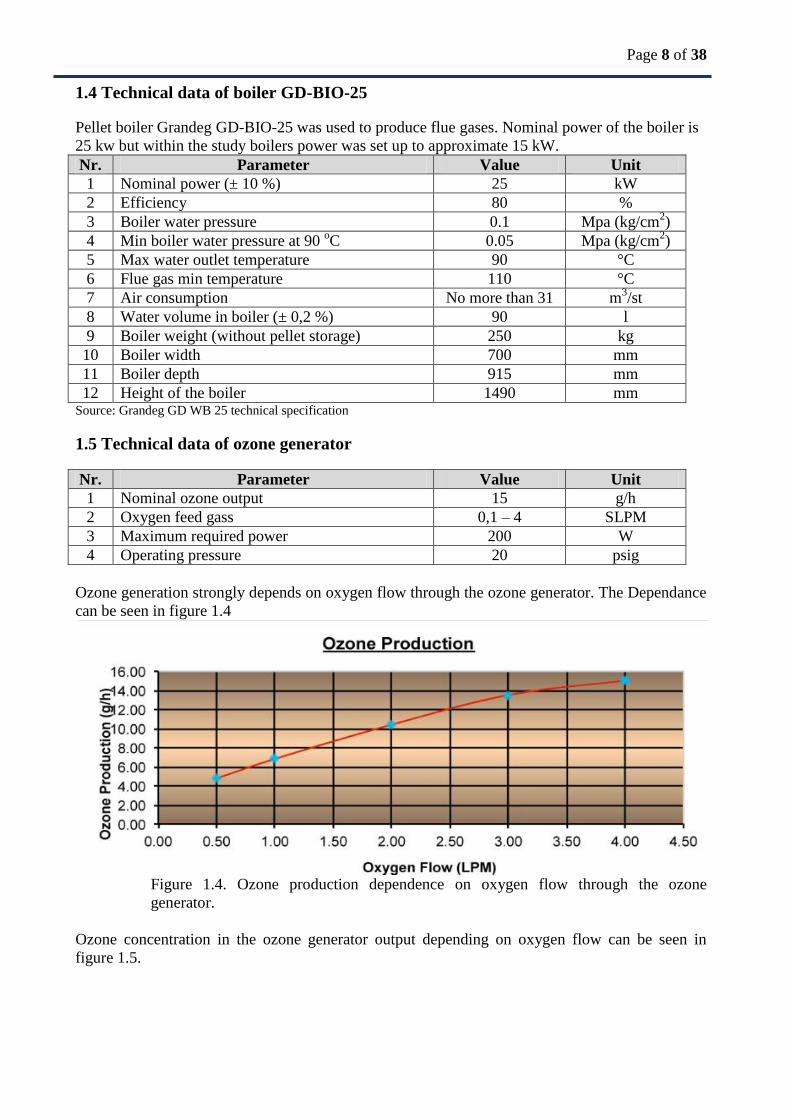
1.5 Technical data of ozone generator
Nr. Parameter Value Unit
1 Nominal ozone output 15 g/h
2 Oxygen feed gass 0,1 – 4 SLPM
3 Maximum required power 200 W
4 Operating pressure 20 psig
Ozone generation strongly depends on oxygen flow through the ozone generator. The Dependance
can be seen in figure 1.4
Figure 1.4. Ozone production dependence on oxygen flow through the ozone
generator.
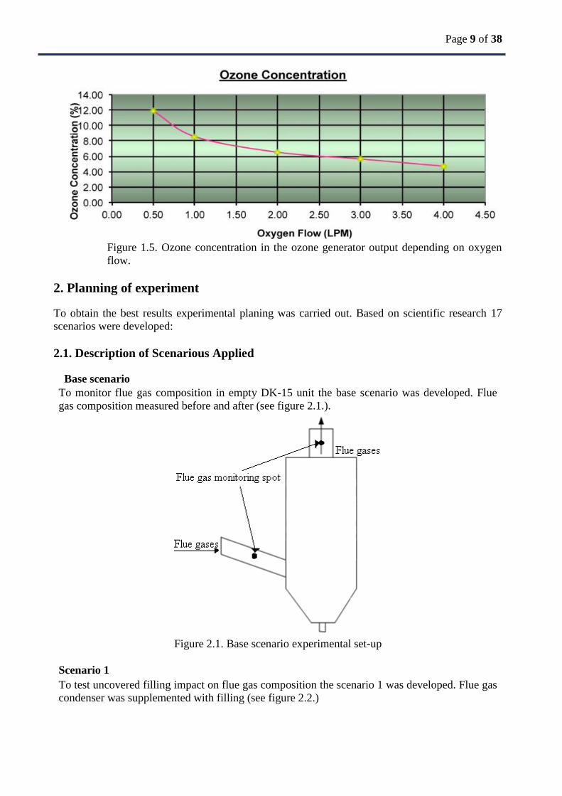
Ozone concentration in the ozone generator output depending on oxygen flow can be seen in
figure 1.5.
Page 9 of 38
Figure 1.5. Ozone concentration in the ozone generator output depending on oxygen
flow.
2. Planning of experiment
To obtain the best results experimental planing was carried out. Based on scientific research 17
scenarios were developed:
2.1. Description of Scenarious Applied
Base scenario
To monitor flue gas composition in empty DK-15 unit the base scenario was developed. Flue
gas composition measured before and after (see figure 2.1.).
Figure 2.1. Base scenario experimental set-up
Scenario 1
To test uncovered filling impact on flue gas composition the scenario 1 was developed. Flue gas
condenser was supplemented with filling (see figure 2.2.)
Page 10 of 38
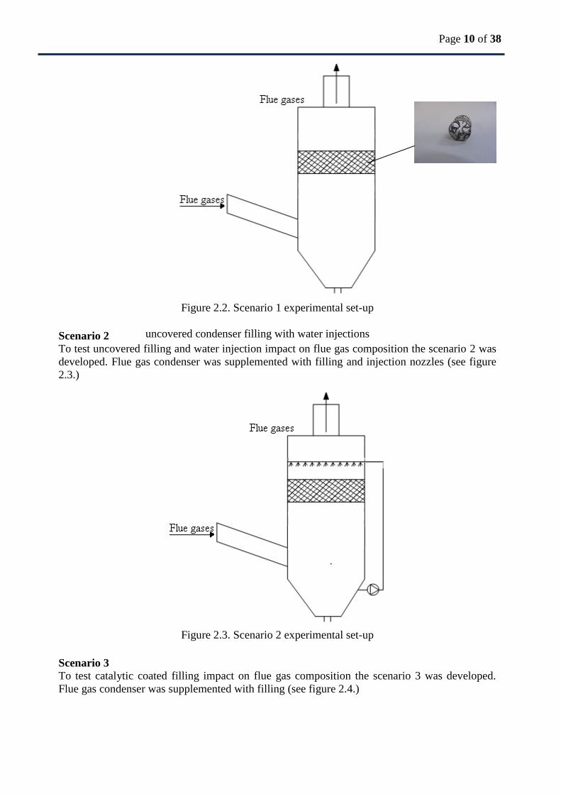
Figure 2.2. Scenario 1 experimental set-up
Scenario 2 uncovered condenser filling with water injections
To test uncovered filling and water injection impact on flue gas composition the scenario 2 was
developed. Flue gas condenser was supplemented with filling and injection nozzles (see figure
2.3.)
Figure 2.3. Scenario 2 experimental set-up
Scenario 3
To test catalytic coated filling impact on flue gas composition the scenario 3 was developed.
Flue gas condenser was supplemented with filling (see figure 2.4.)

Page 11 of 38
Figure 2.4. Scenario 3 experimental set-up
Scenario 4
To test catalytic coated filling and water injection impact on flue gas composition the scenario 4
was developed. Flue gas condenser was supplemented with filling and injection nozzles (see
figure 2.5.)
Figure 2.5. Scenario 4 experimental set-up
Scenario 5
To test catalytic coated filling and water injection at higher temperatures the scenario 5 was
developed. Maximal flue gas output for biomass pellet boiler GD – BIO-25 was used and it was
150 oC. Flue gas condenser was supplemented with filling and injection nozzles (see figure 2.6.)

Page 12 of 38
Figure 2.6. Scenario 5 experimental set-up
Scenario 6
To test catalytic coated filling at higher temperatures the scenario 6 was developed. Maximal
flue gas output for biomass pellet boiler GD – BIO-25 was used and additional heater was used
to raise combustion necessary air inlet temperature. Flue gas condenser was supplemented with
filling (see figure 2.7.)
Figure 2.7. Scenario 6 experimental set-up
Scenario 7
To test catalytic coated filling and water injections at higher temperatures the scenario 7 was
developed. Maximal flue gas output for biomass pellet boiler GD – BIO-25 was used and
additional heater was used to raise combustion necessary air inlet temperature. Flue gas
condenser was supplemented with filling and nozzles (see figure 2.8.)

Page 13 of 38
Figure 2.8. Scenario 7 experimental set-up
Scenario 8
To test ozone impact on flue gas composition and find optimal oxygen flow rate the scenario 8
was developed. Oxygen flow rate was set to 1l/m. Corresponding ozone production was 7 g/h.
Ozone concentration before injection – 8%. Flue gas condenser was supplemented with ozone
injection nozzles (see figure 2.9.)
Figure 2.9. Scenario 8 experimental set-up
Scenario 9
To test ozone impact on flue gas composition and find optimal oxygen flow rate the scenario 9
was developed. Oxygen flow rate was set to 2 l/m. Corresponding ozone production was 10 g/h.
Ozone concentration before injection – 6%. Flue gas condenser was supplemented with ozone
injection nozzles (see figure 2.10.)

Page 14 of 38
Figure 2.10. Scenario 9 experimental set-up
Scenario 10
To test ozone impact on flue gas composition and find optimal oxygen flow rate the scenario 10
was developed. Oxygen flow rate was set to 3 l/m. Corresponding ozone production was 13,5
g/h. Ozone concentration before injection – 6%. Flue gas condenser was supplemented with
ozone injection nozzles (see figure 2.11.)
Figure 2.11. Scenario 10 experimental set-up
Scenario 11
To test ozone impact on flue gas composition and find optimal oxygen flow rate the scenario 11
was developed. Oxygen flow rate was set to 4 l/m. Corresponding ozone production was 15 g/h.
Ozone concentration before injection – 5%. Flue gas condenser was supplemented with ozone

Page 15 of 38
injection nozzles (see figure 2.12.)
Figure 2.12. Scenario 11 experimental set-up
Scenario 12
To test catalytic filling and ozone injection impact on flue gas composition the scenario 12 was
developed. Oxygen flow rate was set to 3 l/m. Corresponding ozone production was 13,5 g/h.
Ozone concentration before injection – 6%. Flue gas condenser was supplemented with ozone
injection nozzles and catalytic filling(see figure 2.13.)
Figure 2.13. Scenario 12 experimental set-up
Scenario 13 The scenario 13 was developed to test sulphur oxide treatment with water injection, catalytic
filling and coated. Water injections 1 l/m were made. Tap water was used. Waste water was
drained to sewage. Flue gas condenser was supplemented with water injection nozzles, catalityc

Page 16 of 38
filling and coated tubes. No circulation through catalitic tubes were obtained (see figure 2.14.).
Figure 2.14. Scenario 13 experimental set-up
Scenario 14 To test water and ozone injection, catalytic filling and catalityc coated tube impact on flue gas
composition the scenario 14 was developed. Water injections 1 l/m and oxygen flow rate was
set to 3 l/m. Corresponding ozone production was 13,5 g/h. Ozone concentration before
injection – 6%. Tap water was used. Waste water was drained to sewage. Flue gas condenser
was supplemented with water, ozone injection nozzles, catalytic filling and catalityc coated
tubes. No circulation through catalitic tubes were obtained (see figure 2.15.).
Figure 2.15. Scenario 14 experimental set-up

Page 17 of 38
Scenario 15 To test water injection, ozone injection, catalytic filling, catalytic coated tubes and flue gas
cooling impact on flue gas composition the scenario 15 was developed. Oxygen flow rate was
set to 3 l/m. Corresponding ozone production was 13,5 g/h. Ozone concentration before
injection – 6%. Injected water was recirculated. Recovered heat energy was measured. Flue gas
condenser was supplemented with water, ozone injection nozzles, catalytic filling and catalityc
coated heat exchanger tubes. Circulation through catalitic tubes was obtained 1,2 m3/h. Heat
exchanger power 2,5 kW (see figure 2.16.).
Figure 2.16. Scenario 15 experimental set-up
Scenario 16
To test water injection, ozone injection, catalytic filling, catalytic coated tubes and flue gas
cooling impact on flue gas composition the scenario 16 was developed. Oxygen flow rate was
set to 3 l/m. Corresponding ozone production was 13,5 g/h. Ozone concentration before
injection – 6%. Injected water was recirculated. Recovered heat energy was measured. Flue gas
condenser was supplemented with water, ozone injection nozzles, catalytic filling and catalityc
coated heat exchanger tubes. Circulation through catalitic tubes was obtained 1,75 m3/h. Heat
exchanger power 2,9 kW (see figure 2.17.).

Page 18 of 38
Figure 2.17. Scenario 16 experimental set-up
Scenario 17
The scenario 17 was developed to test sulphur oxide treatment with water injection, ozone
injection, catalytic filling, catalytic coated tubes and flue gas cooling. GD-BIO-25 fuel was
sprayed with fertilier containing sulpuh oxides. Oxygen flow rate was set to 3 l/m.
Corresponding ozone production was 13,5 g/h. Ozone concentration before injection – 6%.
Injected water was recirculated. Recovered heat energy was measured. Flue gas condenser was
supplemented with water, ozone injection nozzles, catalytic filling and catalityc coated heat
exchanger tubes. Circulation through catalitic tubes was obtained 1,75 m3/h. Heat exchanger
power 2,9 kW (see figure 2.18.).
Figure 2.18. Scenario 17 experimental set-up

Page 19 of 38
2.2. Overview of scenarios
Base scenario Empty experimental device
Scenario 1 Uncovered filling
Scenario 2 uncovered filling and water injection
Scenario 3 Catalytic coated filling
Scenario 4 Catalytic coated filling and water injection
Scenario 5 Catalytic coated filling and water injection. Flue gas temperature 150oC
Scenario 6 Catalytic coated filling 160oC
Scenario 7 Catalytic coated filling and water injection. Flue gas temperature 160oC
Scenario 8 Ozone 1 l/m
Scenario 9 Ozone 2 l/m
Scenario 10 Ozone 3 l/m
Scenario 11 Ozone 4 l/m
Scenario 12 Catalytic filling and ozone 3 l/m
Scenario 13 Water injection, catalytic filling and coated tubes, Sulphur added to fuel.
Scenario 14 Water, ozone injection, catalytic filling and coated tubes
Scenario 15 Water recirculation, ozone injection, catalytic filling, coated tubes and flue
gas cooling. Heat exchanger power 2,5 kW
Scenario 16 Water recirculation, ozone injection, catalytic filling, coated tubes and flue
gas cooling. Heat exchanger power 2,9 kW
Scenario 17 Water recirculation, ozone injection, catalytic filling, coated tubes and flue
gas cooling. Heat exchanger power 2,9 kW. Sulphur added to fuel
3. Tests and Results
Measurements were taken to determine the GD – BIO-25 heat output, efficiency (indirect
method) and DK – 15 condensation heat output, flue gas composition in inlet and outlet, flue gas
temperature, circulation loop temperatures, draught and emission characteristics. The main
concern of tests carried out was NO removal. Tests were carried out with MnO2 and TiO2 mixture
catalyst which was coated on stainless steel tubes with plasma torch. As the powder loses of such
method is very high Aluminum hydroxide was added. First results were obtained by using
condenser filling without any catalyst. Water injections were carried out. Heated water after
sedimentation tank was collected to measure temperature and flow rate therefore power of heat
recovery was determined. Afterwards condenser filling with catalytic coating was implemented.
Tests were made with and without water injections in different temperatures.
Flue gas composition was measured in inlet and outlet. About 90% of NOx consists of NO
and only 10% of NO2. This reports experiments focus on NO measurements and reduction. SO2
(97% from total sulphur oxide concentration) and SO3 (only 3%) measurements were carried out.
3.1 Test setup – measurement methods
OXYGEN, CARBON DIOXIDE, CARBON MONOXIDE, NITROGEN OXIDE AND
SULFUR OXIDE CONTENT: Flue gas analysis was determined by Testo 350 M/Xl and TESTO
350N. O2, CO, NO, NO2, SO2 were measured with electrochemical sensors. Flue gas constituents
were measured through the principle of ion selective potentiometry the sensor contain a
electrolytic matrix that is designed for a specific gas to be detected. Two or three electrodes are
placed in this matrix and an electrical field is applied. Flue gas enters the sensor and chemically
reacts (oxidation or reduction) on the electrode releasing electrically charged particles. This
reaction causes the potential of this electrode to rise or fall with respect to the counter electrode.

Page 20 of 38
With a resistor connected across the electrodes, a current is generated which is proportional to the
concentration of gas present. The output is converted then displayed as a concentration. CO2 was
measured by non dispersive infrared method (NDIR). Each constituent gas in a sample will absorb
some infra red at a particular frequency. By shining an infra-red beam through a sample cell
(containing CO2), and measuring the amount of infra-red absorbed by the sample at the necessary
wavelength, a NDIR detector is able to measure the volumetric concentration of CO2 in the
sample.
FLUE GAS TEMPERATURE: Flue gas temperature was determined using Testo 350 M/Xl as
described in LVS EN 13240. Measurements were made before DK-15 and after.
DATA LOGGING: CampbellSci CR1000 data logging system with AM 16/32 multiplexer, was
used.
DROUGHT: Depression in DK-15 was measured with high accuracy differential pressure gauge
DPT SPAN + / -100, D-AZ. Device pressure range is from -100 Pa to +100 Pa.
HEAT OUTPUT: The heat output from boiler GD – BIO-25 and DK 15 was measured with heat
meters - Kamstrup MP 115 and Danfoss Sonormeter 1000.
BOILER EFFICIENCY: Efficiency was determined with direct calculation method according to
LVS EN 303-5:2001. Fuel consumption, produced heat and calorific value are used in
calculations.
FUEL: The measurements were performed wood pellets from industrial Latvian producer Biogran.
3.2 Fuel parameters
Two kinds of pellets were used. Tests 1-7 was carried out with wood pellets but test0 and tests 8-
16 with straw and wood pellet mixture.
Parameter Unit Value Value
Test fuel -- Wood pellets Wood and straw pellet
mixture (50% - 50%)
Moisture content wt% 8,5 5,58
Ash content wt%, d 0,5 2,34
Highest calorific value as
received
MJ/kg 20,54 18,65
Net calorific value
Length, mean
Diameter, mean
MJ/kg
mm
mm
17,40
19,62
6,5
16,24
16,35
6,6
Durability % 97,4 98,1
3.3 Environmental conditions
Unit Test0 Test1 Test2 Test3 Test4 Test5
Ambient temperature oC 25,4 24,3 25,1 23,6 25,2 25,1
Outside temperature oC -3,6 15,5 14,5 17,2 19 14,2
Air pressure mm 752 785 758 757 757 751
Page 21 of 38
Unit Test6 Test7 Test8 Test9 Test10 Test11
Ambient temperature oC 23,5 25,5 25,4 22,4 24,3 24,7
Outside temperature oC 18,5 19,3 -3,6 -3,2 -2,9 -2,7
Air pressure mm 754 754 752 755 755 767
Unit Test12 Test13 Test14 Test15 Test16 Test17
Ambient temperature oC 23,9 25,1 24,7 23,4 24,1 24,0
Outside temperature oC -3 -3,3 -7,1 -8,2 -6,8 -6,1
Air pressure mm 762 758 755 758 756 756
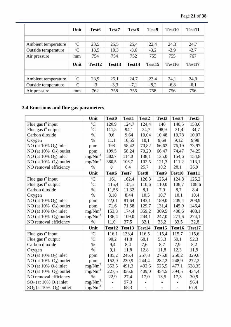
3.4 Emissions and flue gas parameters
Unit Test0 Test1 Test2 Test3 Test4 Test5
Flue gas to input
oC 120,9 124,7 124,4 140 140,5 153,6
Flue gas to output
oC
111,5 94,1 24,7 98,9 31,4 34,7
Carbon dioxide % 9,6 9,64 10,04 10,48 10,78 10,07
Oxygen % 11,1 10,55 10,1 9,69 9,12 9,98
NO (at 10% O2) inlet ppm 198 58,42 70,82 66,62 76,19 73,97
NO (at 10% O2) outlet ppm 199,5 58,24 70,20 66,47 74,47 74,25
NO (at 10% O2) inlet mg/Nm3 382,7 114,0 138,1 135,0 154,6 154,8
NO (at 10% O2) outlet mg/Nm3 380,5 106,7 102,5 121,3 111,2 113,1
NO removal efficiency % 0 6,4 25,7 10,2 28,1 26,9
Unit Test6 Test7 Test8 Test9 Test10 Test11
Flue gas to input
oC 161 162,4 126,3 125,4 124,8 125,2
Flue gas to output
oC
115,4 37,5 110,6 110,0 108,7 108,6
Carbon dioxide % 11,56 11,32 8,1 7,9 8,7 8,4
Oxygen % 8,18 8,44 10,5 10,7 10,1 10,4
NO (at 10% O2) inlet ppm 72,01 81,64 183,1 189,0 209,4 208,9
NO (at 10% O2) outlet ppm 71,6 71,58 129,7 131,4 145,0 146,4
NO (at 10% O2) inlet mg/Nm3 153,3 174,4 359,2 369,5 408,6 408,1
NO (at 10% O2) outlet mg/Nm3 136,4 109,0 244,1 247,0 271,6 274,1
NO removal efficiency % 11,0 37,5 32,1 33,2 33,5 32,8
Unit Test12 Test13 Test14 Test15 Test16 Test17
Flue gas to input
oC 116,1 133,4 116,5 115,4 115,7 115,6
Flue gas to output
oC
90,2 41,8 68,1 55,3 50,1 52,3
Carbon dioxide % 9,4 8,4 7,6 8,7 7,9 8,2
Oxygen % 9,1 11,8 12,8 11,8 12,3 11,9
NO (at 10% O2) inlet ppm 185,2 246,4 257,8 275,8 250,2 329,6
NO (at 10% O2) outlet ppm 152,9 230,9 244,4 282,2 248,9 272,2
NO (at 10% O2) inlet mg/Nm3 353,5 491,3 492,6 525,5 477,1 628,35
NO (at 10% O2) outlet mg/Nm3 227,5 356,6 409,0 454,5 394,5 434,4
NO removal efficiency % 22,9 27,4 17,0 13,5 17,3 30,9
SO2 (at 10% O2) inlet mg/Nm3 - 97,3 - - - 96,4
SO2 (at 10% O2) outlet mg/Nm3 - 68,3 - - - 67,9
Page 22 of 38
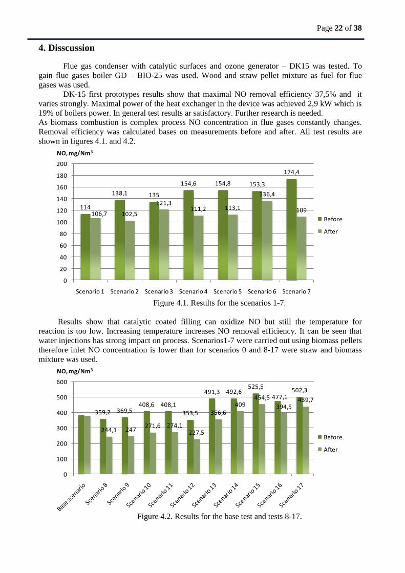
4. Disscussion
Flue gas condenser with catalytic surfaces and ozone generator – DK15 was tested. To
gain flue gases boiler GD – BIO-25 was used. Wood and straw pellet mixture as fuel for flue
gases was used.
DK-15 first prototypes results show that maximal NO removal efficiency 37,5% and it
varies strongly. Maximal power of the heat exchanger in the device was achieved 2,9 kW which is
19% of boilers power. In general test results ar satisfactory. Further research is needed.
As biomass combustion is complex process NO concentration in flue gases constantly changes.
Removal efficiency was calculated bases on measurements before and after. All test results are
shown in figures 4.1. and 4.2.
Figure 4.1. Results for the scenarios 1-7.
Results show that catalytic coated filling can oxidize NO but still the temperature for
reaction is too low. Increasing temperature increases NO removal efficiency. It can be seen that
water injections has strong impact on process. Scenarios1-7 were carried out using biomass pellets
therefore inlet NO concentration is lower than for scenarios 0 and 8-17 were straw and biomass
mixture was used.
Figure 4.2. Results for the base test and tests 8-17.
114
138,1 135
154,6 154,8 153,3
174,4
106,7 102,5
121,3111,2 113,1
136,4
109
0
20
40
60
80
100
120
140
160
180
200
Scenario 1 Scenario 2 Scenario 3 Scenario 4 Scenario 5 Scenario 6 Scenario 7
NO, mg/Nm3
Before
After
359,2 369,5408,6 408,1
353,5
491,3 492,6525,5
477,1502,3
244,1 247271,6 274,1
227,5
356,6409
454,5
394,5439,7
0
100
200
300
400
500
600
NO, mg/Nm3
Before
After

Page 23 of 38
Base scenario results show that NO measurements in empty condenser before and after are
precise. The difference between measurements in empty experimental unit is 0,6%.
Tests 8 to 11 were carried out to test optimal oxygen flow through ozone generator. Results
show that by changing produced ozone amount from 7 to 15 g/h the removal efficiency changes
from 32,1 to 33,5% therefore it is stated that ozone can reduce NO emissions but in experimental
device it is enough to inject 7 g/h. However further experiments were carried out with 13,5 g/h as
it showed maximal removal efficiency 33,5%.
All experimental data strongly varies from input NO concentration and burning process. NO
concentration during tests is shown below:
Scenario 1 was carried out with uncovered filling in experimental device. NO concentration
during experiment is shown in figure 4.3.
Figure 4.3. NO concentration during experiment in first scenario.
Data presented in Figure 4.3 shows that NO concentration in flue gases before experimental
device and after are very similar. Although concentration in flue gases is fluctuating the
fluctuations are equal before and after.
Scenario 2 was carried out with uncovered filling and water injection. NO concentration
during experiment is shown in figure 4.4.
Figure 4.4 NO concentration during experiment in second scenario
0
20
40
60
80
100
120
140
160
0 100 200 300 400 500 600
mg/Nm3 at 10% O2
NObefore NOafter
0
20
40
60
80
100
120
140
160
180
0 100 200 300 400 500 600
mg/Nm3 at 10% O2
NObefore NOafter
Page 24 of 38
Data presented in Figure 4.4 shows that NO concentration in flue gases before experimental
device and after are different. The difference is removed NO emissions by water injection
because previous scenario shows that uncovered filling itself does not make a difference in NO
concentration. Although concentration in flue gases is fluctuating the fluctuations are equal
before and after.
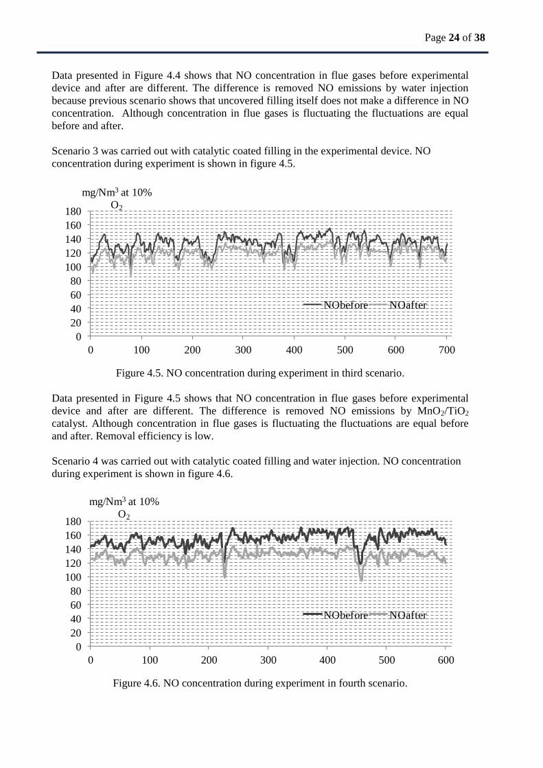
Scenario 3 was carried out with catalytic coated filling in the experimental device. NO
concentration during experiment is shown in figure 4.5.
Figure 4.5. NO concentration during experiment in third scenario.
Data presented in Figure 4.5 shows that NO concentration in flue gases before experimental
device and after are different. The difference is removed NO emissions by MnO2/TiO2
catalyst. Although concentration in flue gases is fluctuating the fluctuations are equal before
and after. Removal efficiency is low.
Scenario 4 was carried out with catalytic coated filling and water injection. NO concentration
during experiment is shown in figure 4.6.
Figure 4.6. NO concentration during experiment in fourth scenario.
0
20
40
60
80
100
120
140
160
180
0 100 200 300 400 500 600 700
mg/Nm3 at 10% O2
NObefore NOafter
0
20
40
60
80
100
120
140
160
180
0 100 200 300 400 500 600
mg/Nm3 at 10% O2
NObefore NOafter

Page 25 of 38
Data presented in Figure 4.6 shows that NO concentration in flue gases before experimental
device and after are different. The difference is removed NO emissions by MnO2/TiO2 catalyst
and water injections. Removal efficiency with water injections and uncovered filling (scenario
2) was 25,7%, but with water injections and catalytic coated filling (scenario 4) 28,1%. The
difference could be explained with catalyst reactions (2,4%).Catalyst efficiency is low because
injected water temperature is around 7oC. Although concentration in flue gases is fluctuating
the fluctuations are equal before and after.
Scenario 5 was carried out with catalytic coated filling and water injection. Flue gas
temperature was raised to 150 oC. NO concentration during experiment is shown in figure 4.7
Figure 4.7. NO concentration during experiment in fifth scenario
Data presented in Figure 4.7 shows that NO concentration in flue gases before experimental
device and after are different. The difference is removed NO emissions by MnO2/TiO2 catalyst
and water injections when flue gas temperature 150oC. Although concentration in flue gases is
fluctuating the fluctuations are equal before and after.
Scenario 6 was carried out with catalytic coated filling. Flue gas temperature was raised to 160 oC. NO concentration during experiment is shown in figure 4.8
Figure 4.8. NO concentration during experiment in sixth scenario.
0
20
40
60
80
100
120
140
160
180
200
0 100 200 300 400 500 600
mg/Nm3 at 10% O2
NObefore NOafter
0
20
40
60
80
100
120
140
160
180
200
0 100 200 300 400 500 600
mg/Nm3at 10% O2
NObefore NOafter

Page 26 of 38
Data presented in Figure 4.8 shows that NO concentration in flue gases before experimental
device and after are different. The difference is removed NO emissions by MnO2/TiO2 catalyst
when flue gas temperature 160oC. Comparing catalyst activities when flue gas temperature
140oC (scenario 3) and 160
oC (scenario 6) it can be concluded that there is a small difference.
Scenario 3 removal efficiency is 10,2% but in scenario 6 removal efficiency is 11,0%.
Although concentration in flue gases is fluctuating the fluctuations are equal before and after.
Scenario 7 was carried out with catalytic coated filling and water injection. Flue gas
temperature was raised to 160 oC. NO concentration during experiment is shown in figure 4.9
Figure 4.9. NO concentration during experiment in seventh scenario.
Data presented in Figure 4.9 shows that NO concentration in flue gases before experimental
device and after are different. The difference is removed NO emissions by MnO2/TiO2 catalyst
and water injections when flue gas temperature 160oC. Comparing removal efficiency in
scenario 5 and scenario 7 it can be concluded that flue gas temperature change by ~10oC
causes removal efficiency increase by 10,6%. Although concentration in flue gases is
fluctuating the fluctuations are equal before and after.
Scenario 8 was carried out with ozone injection. NO concentration during experiment is shown
in figure 4.10
Figure 4.10. NO concentration during experiment in eight scenario.
0
50
100
150
200
250
0 100 200 300 400 500 600
mg/Nm3 at 10% O2
NObefore NOafter
0255075
100125150175200225250275300325350375400425
1 26 51 76 101 126 151 176 201 226
NO at 10% O2, mg/Nm3
Data measurement points
Before
After

Page 27 of 38
Data presented in Figure 4.10 shows that NO concentration in flue gases before experimental
device and after are different. The difference is removed NO emissions by ozone. Injected
ozone amount is set to 7 g/h. Ozone concentration before device is 8%. Although
concentration in flue gases is fluctuating the fluctuations are equal before and after.
Scenario 9 was carried out with ozone injection. NO concentration during experiment is shown
in figure 4.11
Figure 4.11. NO concentration during experiment in ninth scenario
Data presented in Figure 4.11 shows that NO concentration in flue gases before experimental
device and after are different. The difference is removed NO emissions by ozone. Injected
ozone amount is set to 10 g/h. Ozone concentration before device is 6%. Although
concentration in flue gases is fluctuating the fluctuations are equal before and after.
Scenario 10 was carried out with ozone injection. NO concentration during experiment is
shown in figure 4.12
Figure 4.12. NO concentration during experiment in tenth scenario
0255075
100125150175200225250275300325350375400425450
1 26 51 76 101 126 151 176 201 226
NO at 10% O2, mg/Nm3
Data measurement points
Before
After
0255075
100125150175200225250275300325350375400425450475
1 26 51 76 101 126 151 176 201 226
NO at 10% O2, mg/Nm3
Data measurement points
Before
After

Page 28 of 38
Data presented in Figure 4.12 shows that NO concentration in flue gases before experimental
device and after are different. The difference is removed NO emissions by ozone. Injected
ozone amount is set to 13,5 g/h. Ozone concentration before device is 6%. Although
concentration in flue gases is fluctuating the fluctuations are equal before and after.
Scenario 11 was carried out with ozone injection. NO concentration during experiment is
shown in figure 4.13
Figure 4.13. NO concentration during experiment in eleventh scenario
Data presented in Figure 4.13 shows that NO concentration in flue gases before experimental
device and after are different. The difference is removed NO emissions by ozone. Injected
ozone amount is set to 15 g/h. Ozone concentration before device is 6%. Comparing scenarios
8-11 it can be concluded, that ozone is good oxidizer and that there is no high difference in
removal efficiencies when injecting 7-15 g/h of ozone. Although concentration in flue gases is
fluctuating the fluctuations are equal before and after.
Scenario 12 was carried out with catalytic filling and ozone injections. NO concentration
during experiment is shown in figure 4.14
Figure 4.14. NO concentration during experiment in twelfth scenario.
0255075
100125150175200225250275300325350375400425450475
1 26 51 76 101 126 151 176 201 226
NO at 10% O2, mg/Nm3
Data measurement points
Before
After
0255075
100125150175200225250275300325350375400425
1 26 51 76 101 126 151 176 201 226
NO at 10% O2, mg/Nm3
Data measurement points
Before
After

Page 29 of 38
Data presented in Figure 4.14 shows that NO concentration in flue gases before experimental
device and after are different. The difference is removed NO emissions by ozone and catalyst.
At the start of the test higher removal efficiency can be seen. Injected ozone amount is set to
13,5 g/h. Ozone concentration before device is 6%. When using ozone together with catalytic
coated surfaces, removal efficiency is lower than using only ozone. Catalytic coated filling
after ozone injections was installed to increase retention time and to improve ozone/emission
mixing. Scenario 12 shows that catalytic filling after ozone injections does not improve NO
removal efficiency. Although concentration in flue gases is fluctuating the fluctuations are
equal before and after.
Scenario 13 was carried out with water injection, catalytic filling and coated tubes and sulphur
was added to fuel. NO concentration during experiment is shown in figure 4.15
Figure 4.15. NO concentration during experiment in thirteenth scenario
Data presented in Figure 4.15 shows that NO concentration in flue gases before experimental
device and after are different. The difference is removed NO emissions by water injection,
catalytic filling and coated tubes when sulphur is added to fuel. NO removal efficiency was
27,4% but SO2 removal efficiency was 29,8%.
Scenario 14 was carried out with water, ozone injection, catalytic filling and coated tubes. NO
concentration during experiment is shown in figure 4.16
0255075
100125150175200225250275300325350375400425450475500525550575
1 26 51 76 101 126 151 176 201 226 251 276 301
NO at 10 % O2, mg/Nm3
Data measurement points
After
Before

Page 30 of 38
Figure 4.16. NO concentration during experiment in fourteenth scenario.
Data presented in Figure 4.16 shows that NO concentration in flue gases before experimental
device and after are different. The difference is removed NO emissions by water and ozone
injection, catalytic filling and coated tubes.
Scenario 15 was carried out with water recirculation, ozone injection, catalytic filling, coated
tubes and flue gas cooling. NO concentration during experiment is shown in figure 4.17
Figure 4.17. NO concentration during experiment in fifteenth scenario.
Data presented in Figure 4.17 shows that NO concentration in flue gases before experimental
device and after are different. The difference is removed NO emissions by ozone injection,
catalytic filling, coated tubes when water recirculation and flue gas cooling is made. Heat
exchanger power was set to ~ 2,5 kW. NO concentration before and after is fluctuating. It can
be seen that fluctuation trends are inverted. If there is a maximum peak before device then
there is a minimal peak after device.
Scenario 16 was carried out with water recirculation, ozone injection, catalytic filling, coated
tubes and flue gas cooling. NO concentration during experiment is shown in figure 4.18
0255075
100125150175200225250275300325350375400425450475500525550575600
1 26 51 76 101 126 151 176 201 226
NO at 10 % O2, mg/Nm3
Data measurement points
After
Before
0255075
100125150175200225250275300325350375400425450475500525550575600625650675700
1 26 51 76 101 126 151 176 201 226 251 276 301 326 351
NO at 10 % O2, mg/Nm3
Data measurement points
After
Before

Page 31 of 38
Figure 4.18. NO concentration during experiment in sixteenth scenario.
Data presented in Figure 4.17 shows that NO concentration in flue gases before experimental
device and after are different. The difference is removed NO emissions by ozone injection,
catalytic filling, coated tubes when water recirculation and flue gas cooling is made. Heat
exchanger power was set to ~ 2,9 kW. NO concentration before and after is fluctuating. It can
be seen that fluctuation trends are inverted. If there is a maximum peak before device then
there is a minimal peak after device.
Experimental results show that not only NO, SO2 is reduced but also CO emissions are reduced in
the experimental device. Scenario 1 results show that with filling without catalytic coating the CO
emissions are not oxidized but with catalytic surfaces or water injections CO emissions reduces
(see figure 4,19).
Figure 4.19. CO concentration during scenarios 1-7.
Figure 4.19 shows that there is CO removal when using catalytic filling. Higher removal
efficiency can be seen when using water injections, because CO emissions are dissolved in water
solution.
0255075
100125150175200225250275300325350375400425450475500525550575600
1 26
51
76
10
1
12
6
15
1
17
6
20
1
22
6
25
1
27
6
30
1
32
6
35
1
37
6
40
1
42
6
45
1
47
6
50
1
52
6
55
1
57
6
60
1
62
6
65
1
67
6
70
1
NO at 10 % O2, mg/Nm3
Data measurement points
After
Before
401,40
393,57
303,39
438,96
398,66
499,15512,99
398,97
285,03267,73
301,83 302,17
430,04
351,99
0
100
200
300
400
500
600
Scenario 1 Scenario 2 Scenario 3 Scenario 4 Scenario 5 Scenario 6 Scenario 7
CO, mg/Nm3 at 10% O2
Before After

Page 32 of 38
All obtained data were recalculated under the same conditions ( mg/Nm3). Summary of scenario
results can be senn in figure 4.20.
Figure 4.20. Summary of all scenario NO removal efficiencies.
In figure 4.20 all scenario NO removal efficiencies can be seen. Highest removal efficiencies were
observed when using catalytic filling and water injections. Stable results can be seen when using
ozone injections where four scenarios (scenario 8-11) showed very similar results. (32,1 – 33,5%).
It can be concluded that catalyst and ozone in current arrangement does not show synergy effect.
Results indicate that the more components are installed into device the lower is the NO removal
efficiency. Components (catalytical surfaces, ozone or water injections) can oxidize NO emissions
but in complex solution where all components are together additional scientific research is needed.
6,4
25,7
10,2
28,1 26,9
11,0
37,5
32,1 33,2 33,5 32,8
22,9
27,4
17,013,5
17,3
30,9
0
5
10
15
20
25
30
35
40
%
Removal efficiency

Page 33 of 38
Conclusions
1. As biomass combustion is complex process NO concentration in flue gases constantly
changes therefore experimental results vary strongly depending on inlet NO concentration.
Most of the scenarios NO fluctuations are similar before and after experimental device.
2. Results show that catalytic coated filling can oxidize NO but still the temperature for
reaction is too low. Increasing temperature increases NO removal efficiency. Further
experiments with higher temperature have to be done.
3. Removal efficiency with water injections and uncovered filling (scenario 2) was 25,7%,
but with water injections and catalytic coated filling (scenario 4) 28,1%. The difference
could be explained with catalyst reactions (2,4%).Catalyst efficiency is low because
injected water temperature is around 7oC.
4. NO reduction with lower concentrations shows higher removal efficiency. It could be
explained that the catalytic surface are not enough to ensure the same removal rates for
larger amount of emissions.
5. Removal efficiency is lower when catalytic filling after ozone injection is installed. It
could be explained that retention time and ozone/emission mixing does not increase.
6. Experimental results show that not only NO, SO2 is reduced but also CO emissions are
reduced in the experimental device. Results show that with filling without catalytic coating
the CO emissions are not oxidized but with catalytic surfaces or water injections CO
emissions reduces. Higher removal efficiency can be seen when using water injections,
because CO emissions are dissolved in water solution. Results show that SO2 emissions
were reduced by ~29%.
7. It can be concluded that catalyst and ozone in current arrangement does not show synergy
effect. Results indicate that the more components are installed into device the lower is the
NO removal efficiency. Components (catalytical surfaces, ozone or water injections) can
oxidize NO emissions but in complex solution where all components are together
additional scientific research is needed. Device system arrangement has to be optimized to
prevent catalyst inefficient use.
8. Scenarios with flue gas ozonation can reduce NO emissions by at least 30 percent.
Ozone/emission mixing and retention time has to be improved to achieve maximal NO
removal efficiency.
9. Flue gases were cooled to 50oC with indirect heat exchanger which and maximal power in
experiments was achieved 2,9 kW which is 19% of boilers power.

Page 34 of 38
APPENDIX

Page 35 of 38

Page 36 of 38

Page 37 of 38

Page 38 of 38