Adv. Radio Sci., 13, 233–242, 2015

www.adv-radio-sci.net/13/233/2015/

doi:10.5194/ars-13-233-2015

© Author(s) 2015. CC Attribution 3.0 License.

Remote sensing and modeling of energetic electron precipitation

into the lower ionosphere using VLF/LF radio waves and field

aligned current data

E. D. Schmitter1,†

1University of Applied Sciences Osnabrueck, 49076 Osnabrueck, Germany†deceased, 25 March 2015

Correspondence to: M. Förster (mfo@gfz-potsdam.de)

Received: 1 November 2014 – Revised: 30 April 2015 – Accepted: 30 April 2015 – Published: 3 November 2015

Abstract. A model for the development of electron den-

sity height profiles based on space time distributed ioniza-

tion sources and reaction rates in the lower ionosphere is

described. Special attention is payed to the definition of an

auroral oval distribution function for energetic electron en-

ergy input into the lower ionosphere based on a Maxwellian

energy spectrum. The distribution function is controlled by

an activity parameter which is defined proportional to radio

signal amplitude disturbances of a VLF/LF transmitter. Ad-

justing the proportionality constant allows to model precipi-

tation caused VLF/LF signal disturbances using radio wave

propagation calculations and to scale the distribution func-

tion. Field aligned current (FAC) data from the new Swarm

satellite mission are used to constrain the spatial extent of

the distribution function. As an example electron precipita-

tion bursts during a moderate substorm on the 12 April 2014

(midnight–dawn) are modeled along the subauroral propaga-

tion path from the NFR/TFK transmitter (37.5 kHz, Iceland)

to a midlatitude site.

1 Introduction

The lower ionosphere (60–85 km height) is forced from

above by extreme UV, especially Lyman α, solar flare X-

rays and energetic particle precipitation (electrons & 30 keV,

protons & 4 MeV, lower energetic particles do not pene-

trate so deeply). Forcing from below takes place via tides,

gravity- and planetary waves, but also lightning electromag-

netic pulses and upward discharges (Fig. 1). Ionization by

particles not only directly enhances the local electron/ion

Figure 1. Forcing of the lower ionosphere/mesosphere and remote

sensing instrumentation.

density but also leads to the formation of HOx and NOx

molecules. The latter family is rather long living and by ver-

tical transport also reaches the stratosphere where it catalyt-

ically affects the ozone budget, especially in the polar re-

gion (Clilverd et al., 2007; Salmi et al., 2011). This is one

example of the strong coupling of the different ionospheric

and atmospheric layers. Very low frequency and low fre-

quency (VLF/LF) electromagnetic radiation from man made

transmitters (15–60 kHz), but also from lightning, propagates

mainly between ground and the lower ionosphere. The prop-

agation conditions are strongly affected by the conductivity

of the lower ionosphere which is proportional to the quo-

tient of the electron density and collision frequency height

profiles. Remote VLF/LF sensing therefore since decades

proves as an inexpensive and reliable way to assess forc-

ing processes in this layer, also with regard to auroral pre-

Published by Copernicus Publications on behalf of the URSI Landesausschuss in der Bundesrepublik Deutschland e.V.

234 E. D. Schmitter: Remote sensing and modeling of energetic electron precipitation

Figure 2. The monitored propagation path (red line; transmitter:

NRK, receiver: Rx). Also indicated: magnetometers LEIRV: Leir-

vogur, LER: Lerwick; riometers: ABI, SOD, OULU: Abisko, So-

dankyla, Oulu.

cipitation activity (Cummer et al., 1996, 1998). During the

last years we have developed a modeling scheme that al-

lows to assess ionospheric forcing parameters from VLF/LF

amplitude and phase recordings of distant Minimum Shift

Keying (MSK) transmitters (Schmitter, 2010, 2011, 2012,

2013, 2014). As the amplitude of these transmissions is con-

stant, any observed variations are caused along the propaga-

tion path. The monitored propagation path from the VLF/LF

transmitter with the call sign NRK/TFK (37.5 kHz, 63.9◦ N,

22.5◦W, Iceland) to our receiver site 52◦ N, 8◦ E (NW Ger-

many, 2210 km) starts in the subauroral domain and ex-

tends to midlatitudes (Fig. 2). In this paper we extend our

model to include forcing by energetic electrons. The pene-

tration depths of energetic electrons are shown in Fig. 3. As-

suming a Maxwellian electron energy distribution electrons

with a folding energy exceeding 30 keV have their ioniza-

tion maximum in the lower ionosphere (. 85 km) strongly

affecting VLF/LF propagation. Riometers monitor cosmic

noise absorption at about 90–100 km height and in this re-

spect they are also sensitive to electron precipitation, how-

ever with regard to lower energies (∼ 10 keV, i.e. auroral

electrons). Magnetometer recordings reflect the current vari-

ations caused by geomagnetic storm/substorm conditions

which often are accompanied by particle precipitation. Large

scale energetic electron precipitation modify the auroral elec-

trojet and lead to variations of the AL index. In this way

ground based observations by riometers and magnetometers

at proper sites yield important additional information with

regard to the identification of energetic electron precipitation

along the VLF/LF propagation path. The sources of the pre-

Figure 3. Ionization rate vs. height profile for Maxwellian elec-

trons of different folding energies E0 (normalized to the energy

flux rateQ0 = 1 mW m−2= 1 erg cm−2 s−1

= 10−7 J cm−2 s−1=

6.25 · 108 keV cm−2 s−1). Atmospheric model: COSPAR Interna-

tional Reference Atmosphere (CIRA86, June, 50◦ N).

cipitation are the radiation belts (Thorne, 1974; Carson et al.,

2012; Thorne et al., 2013). So, for a detailed characteriza-

tion of precipitation, satellite data are indispensable, even if

a specific domain (e.g. around the VLF/LF propagation path)

cannot be monitored continuously.

Mapping down electric and magnetic field measurements

and derived data (field aligned currents, FACs, Ritter et al.,

2013) from the Swarm satellites yields important information

for the assessment of the energy input into the ionosphere,

particularly with regard to the path and spatial extent of par-

ticle precipitation as well as the acceleration mechanisms.

At least a part of the energetic electron precipitation is cou-

pled to the midnight–dawn region 2 (equatorward) currents

and the dusk–midnight region 1 (poleward) currents (Ohtani

et al., 2010). So it may be expected, that the subauroral VLF

propagation path is mainly affected by energetic electron pre-

cipitation coupled to region 2 (equatorward) field aligned

currents, however compare the discussion of measured FAC

data with regard to this simple picture in Sect. 5. In this paper

we describe the VLF remote sensing procedure followed by

the discussion of our model for the calculation of the electron

density profiles, especially with regard to forcing events like

electron precipitation. After the description of the VLF radio

wave propagation calculations we discuss an example event:

electron precipitation bursts during a moderate substorm on

the 12 April 2014 (midnight–dawn) and the derivation of the

precipitation energy input along a VLF propagation path in

space and time from VLF data as well as using field aligned

current data from the new Swarm satellite mission (launch:

Adv. Radio Sci., 13, 233–242, 2015 www.adv-radio-sci.net/13/233/2015/

E. D. Schmitter: Remote sensing and modeling of energetic electron precipitation 235

22 November 2013). This mission was designed to measure

the magnetic signals from Earth’s core, mantle, crust, oceans,

ionosphere and magnetosphere. It consists of a constellation

of three identical satellites in low polar orbits: two of them

orbit side-by-side, descending from an initial altitude of 460–

300 km over 4 years; the third maintains an altitude of about

530 km. Each satellite carries a vector field magnetometer, an

absolute scalar magnetometer and an electric field instrument

(for a complete description see www.esa.int). In our paper the

field aligned current (FAC) data, a Level 2 product generated

from the magnetic field data, are used.

2 Remote sensing

Remote sensing of lower ionosphere conditions (bottomside

sounding) by monitoring low and very low frequency radio

signal propagation has been a well known method for several

decades. MSK (Minimum Shift Keying) transmitters prove

useful in this respect because of their constant amplitude

emissions. We have analyzed the signal amplitude and phase

variations of the NRK/TFK transmitter (37.5 kHz, 63.9◦ N,

22.5◦W, Iceland) received at a midlatitude site (52◦ N, 8◦ E)

with a great circle distance of 2210 km. The receiver has been

set up with a ferrite coil oriented for maximum signal ampli-

tude of the horizontal magnetic field. After preamplification a

stereo sound card computer interface with 192 kbit sampling

rate is used. The second channel is fed with the 1-s pulse

of a GPS receiver. Our software reads a 170 ms signal train

each second and extracts within the narrow MSK bandwidth

(200 Hz with NRK) amplitude and phase with regard to the

rising GPS-pulse flank yielding a time synchronization better

than 100 ns, corresponding to phase detection errors of 1.4◦

at 37.5 kHz. For the amplitude the signal to noise ratio (SNR)

is recorded. SNR= 0 dB is defined by the averaged signal

level received during transmitter maintenance drop outs. The

time stability of both transmitters proves to be sufficient for

continuous day and night monitoring not only of the ampli-

tude but also of the phase. Our phase detection algorithm for

MSK signals records phases between −90 and +90◦.

The NRK propagation path proceeds most of its way

through the subauroral domain to the midlatitude receiver

site and proves well suited to study lower ionosphere forc-

ing from above by particle precipitation (Schmitter, 2010)

and solar flares (Schmitter, 2013) as well as forcing from be-

low by planetary wave activity (Schmitter, 2011, 2012). In

this paper we concentrate on forcing by energetic electron

precipitation.

3 Modeling electron density profiles

A well known parametrization for the conductivity of the

lower ionosphere (about 60–95 km height) is the two param-

eter model of Wait and Spies (1964) with effective height h′

(km) and profile steepness β (1 / km):

σ(h)= σ0eβ(h−h′), (1)

with σ0 = σ(h= h′)= 2.22 · 10−6 S m−1.

From Eq. (1) together with the collision frequency profile

fc(h)= f0e−h/H , f0 = 1.816 · 1011 Hz and the relation be-

tween conductivity and electron density appropriate for the

very low frequency range σ = ε0ω2

p

fc=

e2ne

mefc(ωp: plasma fre-

quency) we get the classic Wait and Spies (1964) electron

density parametrization of the lower ionosphere:

ne = n0e−h/H eβ(h−h

′), (2)

with n0 = 1.43 · 1013 m−3 and scale height H = 1/0.15=

6.67 km corresponding to an isothermal atmosphere with

T = 230 K.

While this loglinear electron density–height relation often

is a reasonable first order approximation and intuitive with

regard to the interpretation of its two parameters, it does

not explain anything about the physical and chemical pro-

cesses generating the profiles. We therefore want to go a

step further in this respect and use reaction rate equations

describing the development of the density profiles of elec-

trons and ions. Chemical reaction based modeling has been

done in the past at various levels of specification. A very

detailed model of the complex D-layer chemistry is the So-

dankyla Ion Chemistry (SIC) model which takes into account

several hundred reactions and external forcing due to solar

radiation (1–422.5 nm wavelength) as well as particle pre-

cipitation (Verronen et al., 2002). Several approaches have

been made to reduce complexity to most relevant reaction

types – at the cost of introducing effective reaction parame-

ters lumping together different processes. For example: the

14− ion+ electron model of Torkar and Friedrich (1983);

the 6− ion+ electron Mitra–Rowe model (Mitra and Rowe,

1972; Mitra, 1975); the 3− ion+ electron Glukhov–Pasko–

Inan model (Glukhov et al., 1992); the electron “only” model

(Rodger et al., 1998, 2007).

With regard to VLF/LF remote sensing the electron den-

sity profiles are of main interest. For this reason and also to

keep the effort for the propagation calculations tolerable we

use an extended version of the electron “only” model. The

model is extended by taking into account electron detach-

ment reactions. They provide an additional electron source

which gains special importance around dusk and dawn, when

Lyman α radiation is weak. This leads to the following rate

equations for the electron-, positive ion- and negative ion

density distributions, ne, n−, n+ (m−3):

∂ne

∂t= q −αDn+ne−βnne+ (γn+ ρ)n−, (3)

∂n−

∂t=−αin+n−+βnne− (γn+ ρ)n−. (4)

www.adv-radio-sci.net/13/233/2015/ Adv. Radio Sci., 13, 233–242, 2015

236 E. D. Schmitter: Remote sensing and modeling of energetic electron precipitation

Average neutrality is assumed: n+ = ne+ n− and spatial

diffusion is neglected.

– q: ion-pair production (m−3 s−1), during daytime

caused by Lyman α radiation and solar X-rays (from

flares), during nighttime mainly by scattered Lyman

α radiation and cosmic rays. Particle precipitation can

cause additional ionization at any time. See the next

subsection for a detailed discussion.

– αD,i: electron (D) and negative ion (i) recombination co-

efficients (m3 s−1)

– βn: three body attachment coefficient (s−1)

– γn, ρ: coefficients for electron detachment from nega-

tive ions by collision with neutrals or by photons re-

spectively.

The reaction rates depend on the density of the reaction

partners, i.e. the pressure as well as the temperature T (below

100 km height we can assume local thermodynamic equilib-

rium: T = Tneutrals = Tions = Telectrons) . This, as well as rel-

ative abundances of ion species with different recombination

coefficients, means, that the reaction rates vary with height.

We use reaction rates as provided by Brekke (1997), with

the exception of the attachment coefficient βn, where we use

the more detailed relations provided in Rodger et al. (1998,

2007).

All numerical integrations are done using the classic

Runge-Kutta algorithm with variable time step size (0.1, . . .,

2 s).

We now describe the ionization processes in the lower

ionosphere which are included in our model.

3.1 Forcing processes characterizing undisturbed

conditions

Before considering disturbance events the processes gener-

ating the background ionization have to be modeled. In the

lower ionosphere we have continuous forcing from cosmic

radiation and solar Lyman α extreme UV:

– cosmic radiation: the ionization rate is proportional to

the neutral density nn absorbing the radiation:

qcosmic = c0nn, (5)

where c0 increases with geomagnetic latitude (1.2 ·

10−18. . .1.2 · 10−17 s−1 between 0 and 60◦ latitude)

(Nicolet and Aikin, 1960). With undisturbed conditions

cosmic radiation is the main forcing process below

80 km height during the night. During daytime this tran-

sition height drops to 65–70 km.

– solar Lyman α radiation (121.57 nm) on the day side

and night side via scattering:

The Lyman α photon energy of 10.2 eV is high enough

to ionize NO but not the major species O2, N2, so, with

ILα,∞ as the Lyman α intensity incident at the top of the

atmosphere:

qLα = σNO · nNO · ILα,∞e−τ . (6)

ILα,∞ varies with solar activity in the range 2.5, . . .,5 ·

1015 photons s−1 m−2. The optical depth integrated

along the ray path with O2 as the main absorbing species

is:

τ =

∫σO2· nO2

ds. (7)

With Nicolet and Aikin (1960) we use σNO = 2 ·

10−22 m2 for the ionization cross section of NO and

σO2= 10−24 m2 for the absorption cross section of O2

at 121.57 nm. nO2is 0.21 of the total number density

at mesospheric heights. nNO varies considerably: as the

measurements of the Halogen Occultation Experiment

(HALOE) of the Upper Atmosphere Research Satel-

lite (UARS) have shown, the NO number density be-

tween 60 and 90 km height at undisturbed conditions

during the same day can vary at least between 1011 and

1013 m−3 . We adopt 5 · 1012 m−3 as an average undis-

turbed value. The concentration of NO is significantly

enhanced during particle precipitation and for hours af-

terwards (Barth et al., 2001; Saetre et al., 2004) – which

has to be taken into account for the description of pre-

cipitation events during daylight.

3.2 Energetic electron precipitation

With regard to forcing processes leading to disturbed condi-

tions we focus on electron precipitation in this paper. Elec-

trons with energies & 30 keV (Fig. 3) and protons with en-

ergies & 4 MeV penetrate down into the lower ionosphere

(. 85) km. Proton precipitation are mostly confined to the

polar domain, which is not crossed by the propagation path

used in this investigation (Iceland – NW Germany). Different

approaches to predict the auroral oval were summarized by

Sigernes et al. (2011).

With Fang et al. (2008) we model the electron impact ion-

ization rate as

qprecip =Q0

f (E0,ρH)

21εH, (8)

with Q0 (keV cm−3 s−1): total vertically incident electron

flux at the top of the atmosphere.

The fractionf (E0,ρH)

21εHstands for the ionization efficiency

of an electron of (folding) energy E0 at a specific height and

temperature:

Adv. Radio Sci., 13, 233–242, 2015 www.adv-radio-sci.net/13/233/2015/

E. D. Schmitter: Remote sensing and modeling of energetic electron precipitation 237

ρ (g cm−3): atmospheric mass density, H = kTMg

the scale

height in cm at temperature T and with mean atmospheric

molecular mass M , and gravitational acceleration g (to ease

the comparison with literature we use keV and cm units

here).1ε = 35·10−3 keV: mean energy loss per ion pair pro-

duction, E0 (keV): the folding energy of a Maxwellian elec-

tron energy spectrum:

N(E)=Q0

2E30

Ee−E/E0 (9)

N(E) is the differential hemispherical electron number flux

(keV cm−2 s−1).

The numerical evaluation of the energy deposition func-

tion f (E0,ρH) is described in detail in Fang et al. (2008).

We model the incident electron flux Q0 (keV cm−2 s−1)

as a function of the local auroral activity a, geographic lati-

tude, longitude and universal time UT according to Schmitter

(2010):

Q0(a, lat, lon,UT)= c a w2e−

w

2σ2 , (10)

with c = 7.5 · 109 (keV cm−2 s−1). w is a dimensionless dis-

tance parameter with regard to the magnetic pole defined

as follows: with the projected coordinates x = r cos(long),

y = r sin(long), r = re cos(lat), re = 6371 km as compo-

nents of a vector rT = (x,y) we define the vector rn =

RUT(r−rmag pole) which centers the coordinates at the mag-

netic pole and rotates according to the universal time UT

using the usual 2 dimensional rotation matrix with UT ex-

pressed as rotation angle. w = rnT M rn is the bilinear form

of rn scaling these coordinates to an elliptic figure with semi

axes as = (1590+130a) km and bs = (1270+100a) km with

the scaling matrix M= (1/a2s 0;0 1/b2

s ). With this proce-

dure the auroral oval is fixed relative to the longitude of the

sun with the more intensive part at local midnight. As an ex-

ample of this type of distribution function see Fig. 4. Our

approach for modeling the auroral oval distribution can be

compared to that described in Semeniuk et al. (2008). They

use poleward and equatorward boundaries to parametrize the

auroral oval. Our formulation was inspired by the POES au-

roral oval data which made use of an auroral activity param-

eter (this product is replaced by the Ovation–Prime–model,

www.swpc.noaa.gov/models since 14 February 2014). In

contrast to the POES global (hemispheric) activity our activ-

ity parameter quantifies the local precipitation intensity Q0.

The constant c = 7.5 · 109 (keV cm−2 s−1) is defined such

that the elliptic shapes according to the NOAA POES sta-

tistical auroral activity maps (www.swpc.noaa.gov/pmap/)

are reproduced and by integrating Q0 over the hemispheric

area the total hemispheric power input P at auroral ac-

tivity index a = 0, . . .,10 results in accordance with the

NOAA POES data (www.swpc.noaa.gov/ftpdir/lists/hpi/). It

is roughly P = ea/2 GW (GigaWatt).

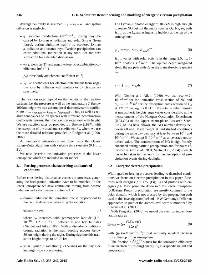
Figure 4. The auroral oval distribution function for 03:00 UT and

POES activity level 10. The two rings mark 60 and 80◦ geographic

latitude. The cross left from the North Pole (center of the rings) is

the magnetic south pole. Colorbar: erg cm−2 s−1=mW m−2. The

VLF propagation path from Iceland to NW Germany (2210 km dis-

tance) is also marked.

The local auroral activity a at time t is parametrized pro-

portional to the VLF/LF amplitude dip:

a(t)= cdB(ampundisturbed− ampdisturbed(t)) (11)

The proportionality constant is measured in auroral activ-

ity units per signal amplitude drop (dB).

3.3 Constraining the precipitation distribution

function using Swarm FAC data

Because the definition of the electron energy input distribu-

tion function Q0 is a main result of this paper we discuss it

in some more detail. For a better understanding we approxi-

mate the oval semi axes parameters as and bs by the circular

average γ = 1380+ 115a km and get

Q0∼= c a

(d

γ

)4

e−

(dγ

)2/2σ 2

, (12)

where d is the distance from the magnetic pole for the ge-

ographic point in question. At at dmax = 2γ σ the function

attains its maximum Q0(dmax)= c a(2σ)4/e2 (e = exp(1)).

The dimensionless width σ is parametrized by σ = σ0+

σ1a(1+ 0.25cos(φUT)) with φUT = 0 at local midnight.

Assuming that electron precipitation is confined to the

range of significant field aligned currents we constrain Q0

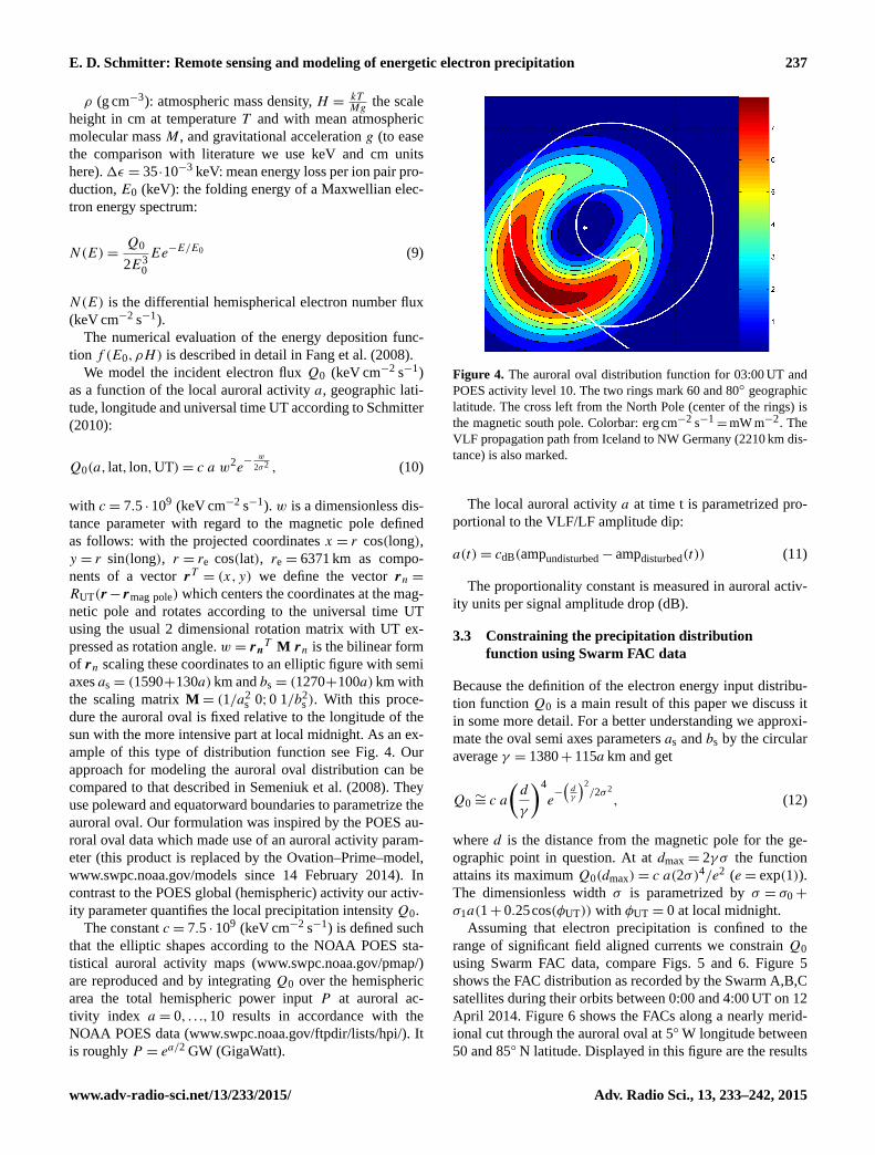
using Swarm FAC data, compare Figs. 5 and 6. Figure 5

shows the FAC distribution as recorded by the Swarm A,B,C

satellites during their orbits between 0:00 and 4:00 UT on 12

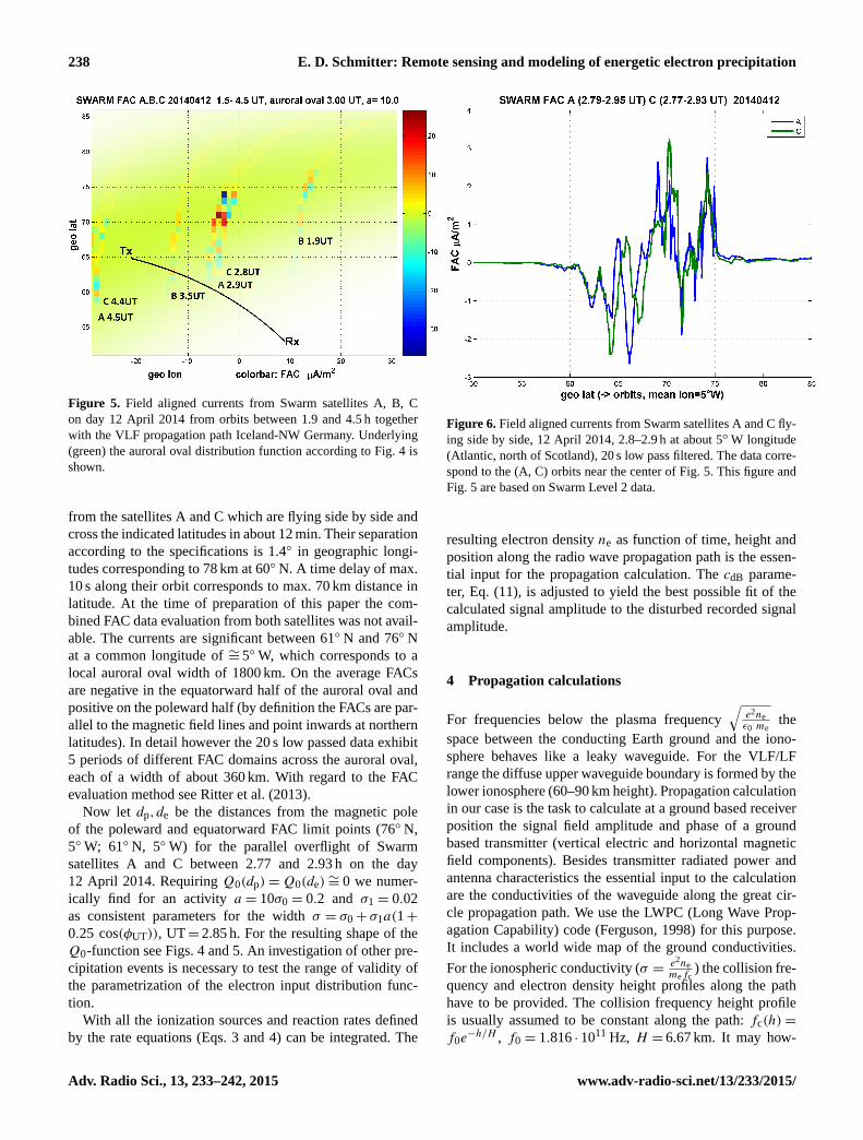
April 2014. Figure 6 shows the FACs along a nearly merid-

ional cut through the auroral oval at 5◦W longitude between

50 and 85◦ N latitude. Displayed in this figure are the results

www.adv-radio-sci.net/13/233/2015/ Adv. Radio Sci., 13, 233–242, 2015

238 E. D. Schmitter: Remote sensing and modeling of energetic electron precipitation

Figure 5. Field aligned currents from Swarm satellites A, B, C

on day 12 April 2014 from orbits between 1.9 and 4.5 h together

with the VLF propagation path Iceland-NW Germany. Underlying

(green) the auroral oval distribution function according to Fig. 4 is

shown.

from the satellites A and C which are flying side by side and

cross the indicated latitudes in about 12 min. Their separation

according to the specifications is 1.4◦ in geographic longi-

tudes corresponding to 78 km at 60◦ N. A time delay of max.

10 s along their orbit corresponds to max. 70 km distance in

latitude. At the time of preparation of this paper the com-

bined FAC data evaluation from both satellites was not avail-

able. The currents are significant between 61◦ N and 76◦ N

at a common longitude of ∼= 5◦W, which corresponds to a

local auroral oval width of 1800 km. On the average FACs

are negative in the equatorward half of the auroral oval and

positive on the poleward half (by definition the FACs are par-

allel to the magnetic field lines and point inwards at northern

latitudes). In detail however the 20 s low passed data exhibit

5 periods of different FAC domains across the auroral oval,

each of a width of about 360 km. With regard to the FAC

evaluation method see Ritter et al. (2013).

Now let dp,de be the distances from the magnetic pole

of the poleward and equatorward FAC limit points (76◦ N,

5◦W; 61◦ N, 5◦W) for the parallel overflight of Swarm

satellites A and C between 2.77 and 2.93 h on the day

12 April 2014. Requiring Q0(dp)=Q0(de)∼= 0 we numer-

ically find for an activity a = 10σ0 = 0.2 and σ1 = 0.02

as consistent parameters for the width σ = σ0+ σ1a(1+

0.25 cos(φUT)), UT= 2.85 h. For the resulting shape of the

Q0-function see Figs. 4 and 5. An investigation of other pre-

cipitation events is necessary to test the range of validity of

the parametrization of the electron input distribution func-

tion.

With all the ionization sources and reaction rates defined

by the rate equations (Eqs. 3 and 4) can be integrated. The

Figure 6. Field aligned currents from Swarm satellites A and C fly-

ing side by side, 12 April 2014, 2.8–2.9 h at about 5◦W longitude

(Atlantic, north of Scotland), 20 s low pass filtered. The data corre-

spond to the (A, C) orbits near the center of Fig. 5. This figure and

Fig. 5 are based on Swarm Level 2 data.

resulting electron density ne as function of time, height and

position along the radio wave propagation path is the essen-

tial input for the propagation calculation. The cdB parame-

ter, Eq. (11), is adjusted to yield the best possible fit of the

calculated signal amplitude to the disturbed recorded signal

amplitude.

4 Propagation calculations

For frequencies below the plasma frequency

√e2ne

ε0 methe

space between the conducting Earth ground and the iono-

sphere behaves like a leaky waveguide. For the VLF/LF

range the diffuse upper waveguide boundary is formed by the

lower ionosphere (60–90 km height). Propagation calculation

in our case is the task to calculate at a ground based receiver

position the signal field amplitude and phase of a ground

based transmitter (vertical electric and horizontal magnetic

field components). Besides transmitter radiated power and

antenna characteristics the essential input to the calculation

are the conductivities of the waveguide along the great cir-

cle propagation path. We use the LWPC (Long Wave Prop-

agation Capability) code (Ferguson, 1998) for this purpose.

It includes a world wide map of the ground conductivities.

For the ionospheric conductivity (σ = e2ne

mefc) the collision fre-

quency and electron density height profiles along the path

have to be provided. The collision frequency height profile

is usually assumed to be constant along the path: fc(h)=

f0e−h/H , f0 = 1.816 · 1011 Hz, H = 6.67 km. It may how-

Adv. Radio Sci., 13, 233–242, 2015 www.adv-radio-sci.net/13/233/2015/

E. D. Schmitter: Remote sensing and modeling of energetic electron precipitation 239

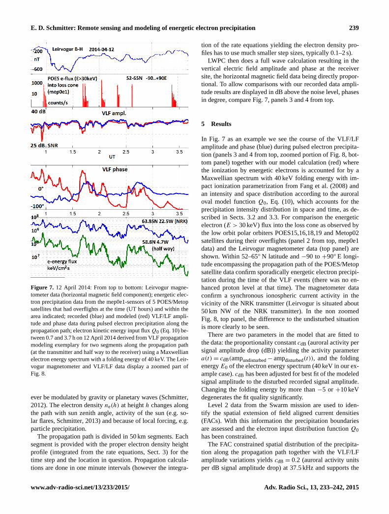
Figure 7. 12 April 2014: From top to bottom: Leirvogur magne-

tometer data (horizontal magnetic field component); energetic elec-

tron precipitation data from the mep0e1-sensors of 5 POES/Metop

satellites that had overflights at the time (UT hours) and within the

area indicated; recorded (blue) and modeled (red) VLF/LF ampli-

tude and phase data during pulsed electron precipitation along the

propagation path; electron kinetic energy input fluxQ0 (Eq. 10) be-

tween 0.7 and 3.7 h on 12 April 2014 derived from VLF propagation

modeling exemplary for two segments along the propagation path

(at the transmitter and half way to the receiver) using a Maxwellian

electron energy spectrum with a folding energy of 40 keV. The Leir-

vogur magnetometer and VLF/LF data display a zoomed part of

Fig. 8.

ever be modulated by gravity or planetary waves (Schmitter,

2012). The electron density ne(h) at height h changes along

the path with sun zenith angle, activity of the sun (e.g. so-

lar flares, Schmitter, 2013) and because of local forcing, e.g.

particle precipitation.

The propagation path is divided in 50 km segments. Each

segment is provided with the proper electron density height

profile (integrated from the rate equations, Sect. 3) for the

time step and the location in question. Propagation calcula-

tions are done in one minute intervals (however the integra-

tion of the rate equations yielding the electron density pro-

files has to use much smaller step sizes, typically 0.1–2 s).

LWPC then does a full wave calculation resulting in the

vertical electric field amplitude and phase at the receiver

site, the horizontal magnetic field data being directly propor-

tional. To allow comparisons with our recorded data ampli-

tude results are displayed in dB above the noise level, phases

in degree, compare Fig. 7, panels 3 and 4 from top.

5 Results

In Fig. 7 as an example we see the course of the VLF/LF

amplitude and phase (blue) during pulsed electron precipita-

tion (panels 3 and 4 from top, zoomed portion of Fig. 8, bot-

tom panel) together with our model calculation (red) where

the ionization by energetic electrons is accounted for by a

Maxwellian spectrum with 40 keV folding energy with im-

pact ionization parametrization from Fang et al. (2008) and

an intensity and space distribution according to the auroral

oval model function Q0, Eq. (10), which accounts for the

precipitation intensity distribution in space and time, as de-

scribed in Sects. 3.2 and 3.3. For comparison the energetic

electron (E > 30 keV) flux into the loss cone as observed by

the low orbit polar orbiters POES15,16,18,19 and Metop02

satellites during their overflights (panel 2 from top, mep0e1

data) and the Leirvogur magnetometer data (top panel) are

shown. Within 52–65◦ N latitude and −90 to +90◦ E longi-

tude encompassing the propagation path of the POES/Metop

satellite data confirm sporadically energetic electron precipi-

tation during the time of the VLF events (there was no en-

hanced proton level at that time). The magnetometer data

confirm a synchronous ionospheric current activity in the

vicinity of the NRK transmitter (Leirvogur is situated about

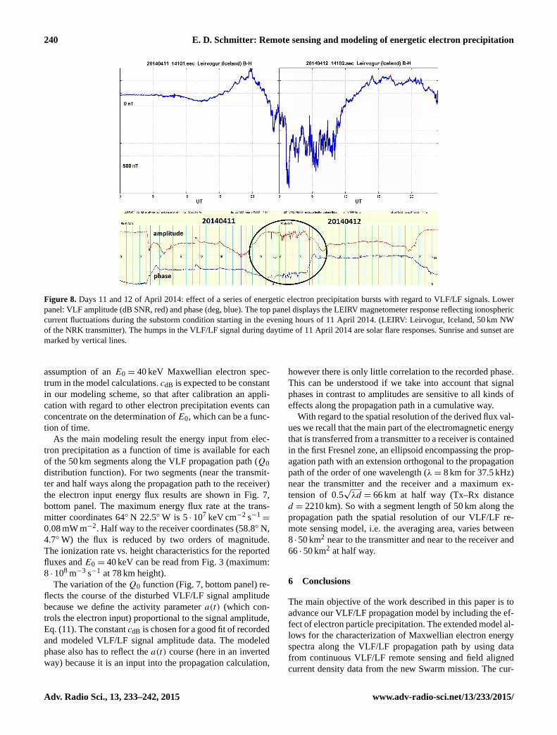
50 km NW of the NRK transmitter). In the non zoomed

Fig. 8, top panel, the difference to the undisturbed situation

is more clearly to be seen.

There are two parameters in the model that are fitted to

the data: the proportionality constant cdB (auroral activity per

signal amplitude drop (dB)) yielding the activity parameter

a(t)= cdB(ampundisturbed− ampdisturbed(t)), and the folding

energyE0 of the electron energy spectrum (40 keV in our ex-

ample case). cdB has been adjusted for best fit of the modeled

signal amplitude to the disturbed recorded signal amplitude.

Changing the folding energy by more than −5 or +10 keV

degenerates the fit quality significantly.

Level 2 data from the Swarm mission are used to iden-

tify the spatial extension of field aligned current densities

(FACs). With this information the precipitation boundaries

are assessed and the electron input distribution function Q0

has been constrained.

The FAC constrained spatial distribution of the precipita-

tion along the propagation path together with the VLF/LF

amplitude variations yields cdB = 0.2 (auroral activity units

per dB signal amplitude drop) at 37.5 kHz and supports the

www.adv-radio-sci.net/13/233/2015/ Adv. Radio Sci., 13, 233–242, 2015

240 E. D. Schmitter: Remote sensing and modeling of energetic electron precipitation

Figure 8. Days 11 and 12 of April 2014: effect of a series of energetic electron precipitation bursts with regard to VLF/LF signals. Lower

panel: VLF amplitude (dB SNR, red) and phase (deg, blue). The top panel displays the LEIRV magnetometer response reflecting ionospheric

current fluctuations during the substorm condition starting in the evening hours of 11 April 2014. (LEIRV: Leirvogur, Iceland, 50 km NW

of the NRK transmitter). The humps in the VLF/LF signal during daytime of 11 April 2014 are solar flare responses. Sunrise and sunset are

marked by vertical lines.

assumption of an E0 = 40 keV Maxwellian electron spec-

trum in the model calculations. cdB is expected to be constant

in our modeling scheme, so that after calibration an appli-

cation with regard to other electron precipitation events can

concentrate on the determination of E0, which can be a func-

tion of time.

As the main modeling result the energy input from elec-

tron precipitation as a function of time is available for each

of the 50 km segments along the VLF propagation path (Q0

distribution function). For two segments (near the transmit-

ter and half ways along the propagation path to the receiver)

the electron input energy flux results are shown in Fig. 7,

bottom panel. The maximum energy flux rate at the trans-

mitter coordinates 64◦ N 22.5◦W is 5 · 107 keV cm−2 s−1=

0.08 mW m−2. Half way to the receiver coordinates (58.8◦ N,

4.7◦W) the flux is reduced by two orders of magnitude.

The ionization rate vs. height characteristics for the reported

fluxes and E0 = 40 keV can be read from Fig. 3 (maximum:

8 · 108 m−3 s−1 at 78 km height).

The variation of theQ0 function (Fig. 7, bottom panel) re-

flects the course of the disturbed VLF/LF signal amplitude

because we define the activity parameter a(t) (which con-

trols the electron input) proportional to the signal amplitude,

Eq. (11). The constant cdB is chosen for a good fit of recorded

and modeled VLF/LF signal amplitude data. The modeled

phase also has to reflect the a(t) course (here in an inverted

way) because it is an input into the propagation calculation,

however there is only little correlation to the recorded phase.

This can be understood if we take into account that signal

phases in contrast to amplitudes are sensitive to all kinds of

effects along the propagation path in a cumulative way.

With regard to the spatial resolution of the derived flux val-

ues we recall that the main part of the electromagnetic energy

that is transferred from a transmitter to a receiver is contained

in the first Fresnel zone, an ellipsoid encompassing the prop-

agation path with an extension orthogonal to the propagation

path of the order of one wavelength (λ= 8 km for 37.5 kHz)

near the transmitter and the receiver and a maximum ex-

tension of 0.5√λd = 66 km at half way (Tx–Rx distance

d = 2210 km). So with a segment length of 50 km along the

propagation path the spatial resolution of our VLF/LF re-

mote sensing model, i.e. the averaging area, varies between

8 ·50 km2 near to the transmitter and near to the receiver and

66 · 50 km2 at half way.

6 Conclusions

The main objective of the work described in this paper is to

advance our VLF/LF propagation model by including the ef-

fect of electron particle precipitation. The extended model al-

lows for the characterization of Maxwellian electron energy

spectra along the VLF/LF propagation path by using data

from continuous VLF/LF remote sensing and field aligned

current density data from the new Swarm mission. The cur-

Adv. Radio Sci., 13, 233–242, 2015 www.adv-radio-sci.net/13/233/2015/

E. D. Schmitter: Remote sensing and modeling of energetic electron precipitation 241

rent status of the modeling efforts has been demonstrated

with regard to electron precipitation bursts during a mod-

erate substorm condition on 12 April 2014 (Kp= 5, min.

DST=−80 nT, min. AL=−700 nT). Signal amplitude dis-

turbances along a 37.5 kHz radio propagation path from Ice-

land (63.9◦ N, 22.5◦W) to a midlatitude site (52◦ N, 8◦ E)

have been modeled successfully and an electron energy input

distribution function has been derived. Future work intends

to model many different precipitation events and to further

validate the parametrization of the electron input distribution

function. For this purpose our software has to be optimized

with regard to speed to allow for faster modeling cycles. The

space time characterization of electron energy spectra can

help to quantify the effectiveness of energetic electron pre-

cipitation with regard to NOx production and ozone deple-

tion at mesospheric heights, underlining the importance of

energetic electron precipitation as a part of solar influence

on the atmosphere and the climate system (Andersson et al.,

2014).

Acknowledgements. Swarm Level 2 data have been provided

by the European Space Agency and the POES/Metop data have

been provided by the US NOAA National Geophysical Data Center.

Edited by: M. Förster

Reviewed by: two anonymous referees

References

Andersson, M. E., Verronen, P. T., Rodger, C. J., Clilverd, M. A.,

and Seppaelae, A.: Missing driver in the SunEarth connection

from energetic electron precipitation impacts mesospheric ozone,

Nat. Comm., 5, 5197, doi:10.1038/ncomms6197, 2014.

Barth, C. A., Baker, D. N., Mankoff, K. D., and Bailey, S. M.: The

northern auroral region as observed in nitric oxide, Geophys.

Res. Lett., 8, 1463–1466, doi:10.1029/2000GL012649, 2001.

Brekke, A.: Physics of the upper polar atmosphere, John Wiley &

Sons, New York, USA, 1997.

Carson, B. R., Rodger, C. J., and Clilverd, M. A.: POES satellite

observations of EMIC-wave driven relativistic electron precipi-

tation during 1998–2010, J. Geophys. Res.-Space, 118, 232–243,

doi:10.1029/2012JA017998, 2012.

Clilverd, M. A., Seppaelae, A., Rodger, C. J., Thomson, N. R.,

Lichtenberger, J., and Steinbach, P.: Temporal variability of the

descent of high-altitude NOX inferred from ionospheric data, J.

Geophys. Res., 112, A09307, doi:10.1029/2006JA012085, 2007.

Cummer, S. A., Bell, T. F., and Inan, U. S.: VLF remote sensing of

the auroral electrojet, J. Geophys. Res., 101, 5381–5389, 1996.

Cummer, S. A., Inan, U. S., and Bell, T. F.: Ionospheric D region

remote sensing using VLF radio atmospherics, Radio Sci., 33,

1781–1792, doi:10.1029/98RS02381, 1998.

Fang, X., Randal, C. E., Lummerzheim, I. D., Solomon, S. C.,

Mills, M. J., Marsh, D. R., Jackman, C. H., Wang, W., and

Lu, G.: Electron impact ionization: A new parameterization for

100 eV to 1 MeV electrons, J. Geophys. Res., 113, A09311,

doi:10.1029/2008JA013384, 2008.

Ferguson, J. A.: Computer Programs for Assessments of Long-

Wavelength Radio Communications, Version 2.0, Technical Doc-

ument, SPAWAR Systems Center, San Diego, USA, available at:

http://www.dtic.mil/dtic/tr/fulltext/u2/a350375.pdf (last access:

12 May 2015), 1998.

Glukhov, V. S., Pasko, V. P., and Inan, U. S.: Relaxation of

transient lower ionospheric disturbances caused by lightning-

whistler-induced electron precipitation bursts, J. Geophys. Res.,

97, 16971–16979, 1992.

Mitra, A. P. and Rowe, J. N.: Ionospheric effects of solar flares – VI.

Changes in D-region ion chemistry during solar flares, J. Atmos.

Sol.-Terr. Phy., 34, 795–806, 1972.

Mitra, A. P.: D-region in disturbed conditions, including flares and

energetic particles, J. Atmos. Sol.-Terr. Phy., 37, 895–913, 1975.

Nicolet, M. and Aikin, A. C.: The Formation of the D Region of the

Ionosphere, J. Geophys. Res., 65, 1469–1483, 1960.

Ohtani, S., Wing, S., Newell, P. T., and Higuchi, T.: Lo-

cations of nights’ side precipitation boundaries relative to

R2 and R1 currents, J. Geophys. Res., 115, A10233,

doi:10.1029/2010JA015444, 2010.

Ritter, P., Lühr, H., and Rauberg, J.: Determining field-aligned cur-

rents with the Swarm constellation mission, Earth Planets Space,

65, 1285–1294, 2013.

Rodger, C. J., Molchanov, O. A., and Thomson, N. R.: Relaxation

of transient ionization in the lower ionosphere, J. Geophys. Res.,

103, 6969–6975, 1998.

Rodger, C. R., Clilverd, M. A., Thomson, N. R., Gamble, R. J., Sep-

paelae, A., Turunen, E., Meredith, N. P., Parrot, M., Sauvaud, J.

A., Berthelier, J. J.: Radiation belt electron precipitation into the

atmosphere: Recovery from a geomagnetic storm, J. Geophys.

Res., 112, A11307, doi:10.1029/2007JA012383, 2007.

Saetre, C., Stadsnes, J., Nesse, H., Aksnes, A., Petrinec, S. M.,

Barth, C. A., Baker, D. N., Vondrak, R. R., and Ostgaard, N.: En-

ergetic electron precipitation and the NO abundance in the upper

atmosphere: A direct comparison during a geomagnetic storm, J.

Geophys. Res., 109, A09302, doi:10.1029/2004JA010485, 2004.

Salmi, S.-M., Verronen, P. T., Thölix, L., Kyrölä, E., Backman, L.,

Karpechko, A. Yu., and Seppälä, A.: Mesosphere-to-stratosphere

descent of odd nitrogen in February-March 2009 after sudden

stratospheric warming, Atmos. Chem. Phys., 11, 4645–4655,

doi:10.5194/acp-11-4645-2011, 2011.

Semeniuk, K., McConnell, J. C. , Jin, J. J. Jarosz, J. R., Boone,

C. D., and Bernath, P. F.: N2O production by high energy au-

roral electron precipitation, J. Geophys. Res., 113, D16302,

doi:10.1029/2007JD009690, 2008.

Schmitter, E. D.: Remote auroral activity detection and modeling

using low frequency transmitter signal reception at a midlati-

tude site, Ann. Geophys., 28, 1807–1811, doi:10.5194/angeo-28-

1807-2010, 2010.

Schmitter, E. D.: Remote sensing planetary waves in the midlatitude

mesosphere using low frequency transmitter signals, Ann. Geo-

phys., 29, 1287–1293, doi:10.5194/angeo-29-1287-2011, 2011.

Schmitter, E. D.: Data analysis of low frequency transmitter signals

received at a midlatitude site with regard to planetary wave activ-

ity, Adv. Radio Sci., 10, 279–284, doi:10.5194/ars-10-279-2012,

2012.

Schmitter, E. D.: Modeling solar flare induced lower ionosphere

changes using VLF/LF transmitter amplitude and phase ob-

www.adv-radio-sci.net/13/233/2015/ Adv. Radio Sci., 13, 233–242, 2015

242 E. D. Schmitter: Remote sensing and modeling of energetic electron precipitation

servations at a midlatitude site, Ann. Geophys., 31, 765–773,

doi:10.5194/angeo-31-765-2013, 2013.

Schmitter, E. D.: Remote sensing and modeling of lightning

caused long recovery events within the lower ionosphere using

VLF/LF radio wave propagation, Adv. Radio Sci., 12, 241-250,

doi:10.5194/ars-12-241-2014, 2014.

Sigernes, F., Dyrland, M., Brekke, P., Chernouss, S., Lorentzen,

D. A., Oksavik, K., and Deehr, C. S.: Two methods

to forecast auroral displays, J. Space Weather, 1, A03,

doi:10.1051/swsc/2011003, 2011.

Thorne, R. M.: A cause of dayside relativistic electron possible

precipitation events, J. Atmos. Sol.-Terr. Phy., 36, 635–645,

doi:10.1016/0021-9169(74)90087-7, 1974.

Thorne, R. M., Li, W., Ni, B., Ma, Q., Bortnik, J., Chen, L., Baker,

D. N., Spence, H. E., Reeves, G. D., Henderson, M. G., Kletzing,

C. A., Kurth, W. S., Hospodarsky, G. B., Blake, J. B., Fennell, J.

F., Claudepierre, S. G., and Kanekal, S. G.: Rapid local accel-

eration of relativistic radiation-belt electrons by magnetospheric

chorus, Nature, 504, 411–414, doi:10.1038/nature12889, 2013.

Torkar, K. and Friedrich, M.: Tests of an Ion-Chemical Model of

the D- and Lower E-Region, J. Atmos. Terr. Phys., 45, 369–385,

1983.

Verronen, P. T., Turunen, E., Ulich, T., and Kyrola, E.: Modelling

the effects of the October 1989 solar proton event on mesospheric

odd nitrogen using a detailed ion and neutral chemistry model,

Ann. Geophys., 20, 1967–1976, 2002,

http://www.ann-geophys.net/20/1967/2002/.

Wait, J. R. and Spies, K. P.: Characteristics of the Earth-

ionosphere waveguide for VLF radio waves, NBS Tech.

Note 300, available at: http://nova.stanford.edu/~vlf/IHY_Test/

Tutorials/SfericsAndTweaks/Papers/Wait1964f.pdf (last access:

12 May 2015), 1964.

Adv. Radio Sci., 13, 233–242, 2015 www.adv-radio-sci.net/13/233/2015/