Reliability Optimization of Series-Parallel Systems Using a Genetic Algorithm

David W. Coit, IEEE Student Member

Alice E. Smith1, IEEE Member

University of PittsburghPittsburgh, PA 15261

To appear March 1996, IEEE Transactions on Reliability, vol. 45, no. 1

1 Corresponding author.

1

Reliability Optimization of Series-Parallel Systems Using a Genetic Algorithm

Key Words - Genetic algorithm, Combinatorial optimization, Redundancy allocation problem,

Reliability design

Summary & Conclusions - A problem specific genetic algorithm (GA) is developed and

demonstrated to analyze series-parallel systems and to determine the optimal design configuration when

there are multiple component choices available for each of several k-out-of-n:G subsystems. The

problem is to select components and levels of redundancy to optimize some objective function given

system level constraints on reliability, cost and/or weight. Previous formulations of the problem have

implicit restrictions concerning the type of redundancy allowed, the number of available component

choices and whether mixing of components is allowed. The GA used to analyze this problem is a robust

evolutionary optimization search technique with very few restrictions concerning the type or size of the

design problem. The solution approach was to solve the dual of a nonlinear optimization problem by

using a dynamic penalty function. The GA was demonstrated to perform very well on two types of

problems, the redundancy allocation problem originally proposed by Fyffe, Hines and Lee and a second,

randomly generated problem with more complex k-out-of-n:G configurations.

1. INTRODUCTION

This paper describes the use of a genetic algorithm (GA) to determine solutions to the redundancy

allocation problem for a series-parallel system. In this problem formulation, there is a specified number of

subsystems and, for each subsystem, there are multiple component choices which can be selected, with

replacement, and used in parallel. For those systems designed using off-the-shelf component types, with

known cost, reliability and weight, system design and component selection becomes a combinatorial

2

optimization problem. The consumer electronics industry is one such example where new system designs

are composed largely of standard component types (e.g., microcircuits, transistors, resistors) with known

characteristics. The problem is then to select the optimal combination of parts and levels of redundancy

to collectively meet reliability and weight constraints at a minimum cost, or alternatively, to maximize

reliability given cost and weight constraints. The series-parallel system with k-out-of-n:G subsystem

redundancy, addressed in this paper, is a common representation for many system design problems.

The GA optimization approach was used in this research. It is one of a family of heuristic

optimization techniques, which also include simulated annealing, Tabu search and evolutionary strategies

[1]. GAs have been demonstrated to converge to the optimal solution for many diverse difficult

problems, although optimality cannot be guaranteed. The ability of the GA to efficiently find good

solutions often depends on properly customizing the encoding, breeding operators and fitness measures

to the specific engineering problem.

1.1 Previous Research in the Redundancy Allocation Problem

The redundancy allocation problem for series-parallel systems has proven to be difficult. Chern

[2] showed that the problem is NP-hard. Different optimization approaches to determine optimal or

“very good” solutions have included dynamic programming, integer programming, mixed integer and

nonlinear programming, and heuristics. An overview and summary of work in this area is presented in

Tillman, Hwang and Kuo [3, 4].

Bellman [5] and Bellman and Dreyfus [6, 7] used dynamic programming to maximize reliability

for a system given a single cost constraint. For each subsystem, there was only one component choice so

the problem was to identify the optimal levels of redundancy. Fyffe, Hines and Lee [8] also used a

dynamic programming approach and solved a more difficult design problem. They considered a system

with 14 subsystems and constraints on both cost and weight. For each subsystem, there were three or

3

four different component choices each with different reliability, cost and weight. To accommodate

multiple constraints, they used a Lagrangian multiplier within the objective function. While their

formulation provided a selection of different components, the search space was artificially restricted to

only consider solutions where identical components are in parallel.

Nakagawa and Miyazaki [9] showed that the use of a Lagrangian multiplier with dynamic

programming is often inefficient. Instead of Lagrangian multipliers, they deployed a surrogate constraints

approach. Their algorithm was demonstrated by solving 33 different variations of the Fyffe problem. Of

the 33 problems, their N&M algorithm produced optimal solutions to 30 of these problems. For the

other cases, the algorithm did not lead to a feasible solution.

A second approach has been to use integer programming. To use integer programming, it is

necessary to artificially restrict the search space and prohibit mixing of different components within a

subsystem. For problems to maximize reliability given nonlinear but separable constraints, many

variations of the problem can be transformed into an equivalent integer programming problem. This was

demonstrated by Ghare and Taylor [10], who used a branch-and-bound approach. Bulfin and Liu [11]

also used integer programming. They formulated the problem as a knapsack problem using surrogate

constraints (approximated by Lagrangian multipliers found by subgradient optimization [12]). They

formulated the Fyffe problem and its variations as integer programs and determined the optimal solution

to all 33 problems investigated by Nakagawa and Miyazaki. They only solved problems with 1-out-of-n:G

subsystem redundancy.

Other examples of integer programming solutions are described by Misra and Sharma [13], Gen,

Ida, Tsujimura and Kim [14] and Gen, Ida and Lee [15]. Misra and Sharma present a fast algorithm to

solve integer programming problems like those of Ghare and Taylor [10]. The latter two papers

formulate the problem as a multi-objective decision making problem with distinct goals for reliability, cost

4

and weight.

There have been several effective uses of mixed integer and nonlinear programming to solve the

redundancy allocation problem. Several notable examples are Tillman, Hwang and Kuo [16, 17]. In

these problems, component reliability is treated as a continuous variable and component cost is expressed

as a function of reliability and other parameters.

While the redundancy allocation problem has been studied in great detail, two areas which have

not been sufficiently analyzed are the implications of mixing functionally similar components within a

parallel subsystem and the use of k-out-of-n:G redundancy (with k > 1). In practice many system designs

use multiple different (yet functionally similar) components in parallel. For example, airplanes often use a

primary electronic gyroscope and a secondary mechanical gyroscope working in parallel, and most new

automobiles have a redundant, i.e., spare, tire with different size and weight characteristics forming a 4-

out-of-5:G standby redundant system. The power of a GA is that it can easily be adapted to many

diverse design scenarios including those with mixing of components, k-out-of-n:G redundancy and more

complex forms of redundancy.

1.2 Previous Use of Genetic Algorithms to Solve Reliability Problems

GAs have been used to solve many difficult engineering problems and are particularly effective for

combinatorial optimization problems with large and complex search spaces. Within the reliability field,

however, there has been very few examples of their use. For a fixed design configuration and known

incremental decreases in component failure rates and their associated costs, Painton and Campbell [18,

19] used a GA to find maximum reliability solutions to satisfy specific cost constraints. Their algorithm is

flexible and can be formulated to optimize reliability, mean time between failure (MTBF), the 5th

percentile of the MTBF distribution or availability. Ida, Gen and Yokota [20] used a GA to find

solutions to a redundancy allocation problem where there are several failure modes. This problem had

5

previously been solved by both nonlinear programming and integer programming. Coit and Smith [21]

analyzed a series-parallel system with eight subsystems and ten unique component choices for each

subsystem. The search space investigated had > 1030 unique solutions and the GA would readily

converge to a solution after analyzing less than 4 x 10-24% of the search space. An interesting feature of

this work is that neural network approximations to subsystem reliability, instead of exact solutions, were

used.

2. NOTATION AND ASSUMPTIONS

2.1 Notation

R reliability constraint

C cost constraint

W weight constraint

s number of subsystems

mi number of available component choices for subsystem i (i = 1,...,s)

rij reliability of component j available for subsystem i

cij cost of component j available for subsystem i

wij weight of component j available for subsystem i

xij number of the jth component used in subsystem i

xi (xi1, xi2, ..., xi,mi)

tj number of good (not failed) of jth component

t (t1, t2, ..., tmi)

ni total number of components used in subsystem i

= xi1 + xi2 + ... + xi,mi

nmax maximum number of components in parallel (user specified)

ki minimum number of components in parallel required for subsystem i to operate

k (k1, k2, ..., ks)

Ri(xi|ki) reliability of subsystem i, given ki

Ci(xi) total cost of subsystem i

6

Wi(xi) total weight of subsystem i

vq vector encoding of solution q

p population size

λ Lagrangian multiplier vector

P(λ,vq) penalty function for qth member of the population

f(λ,vq) fitness for qth member of the population

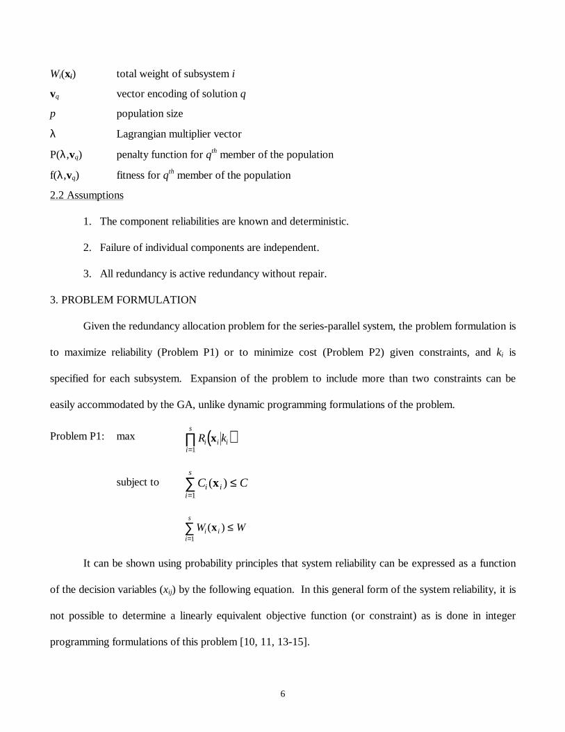
2.2 Assumptions

1. The component reliabilities are known and deterministic.

2. Failure of individual components are independent.

3. All redundancy is active redundancy without repair.

3. PROBLEM FORMULATION

Given the redundancy allocation problem for the series-parallel system, the problem formulation is

to maximize reliability (Problem P1) or to minimize cost (Problem P2) given constraints, and ki is

specified for each subsystem. Expansion of the problem to include more than two constraints can be

easily accommodated by the GA, unlike dynamic programming formulations of the problem.

Problem P1: max ( )R ki i ii

s

x=

∏1

subject to C Ci ii

s

( )x=∑ ≤

1

W Wi ii

s

( )x=∑ ≤

1

It can be shown using probability principles that system reliability can be expressed as a function

of the decision variables (xij) by the following equation. In this general form of the system reliability, it is

not possible to determine a linearly equivalent objective function (or constraint) as is done in integer

programming formulations of this problem [10, 11, 13-15].

7

( )

( )

R R k

x

tr r

s i ii

s

ij

jj

m

t lj

l

k

ijt

ij

x t

i

s i

j

m

ij

ij j

i

( )x ,x ,...x k x

t

1 2 s i=

= −

−

=

==

=

=

− −

=

∏

∏∑∑∏∑

1

1

1

0

1

1

1 1 (1)

Within the two problem formulations, system weight and cost are often defined as linear functions

primarily because this is a reasonable representation of the cumulative effect of component cost and

weight. In the examples which follow in Section 5.0, cost and weight are assumed to be linear, however

this is not a requirement. Nonlinear constraints and even nonseparable constraints can be handled by the

GA, unlike integer programming formulations where constraints must be separable.

The size of the search space (N) is very large even for small and moderately sized problems.

Assuming an upper bound on the number of redundant components (nmax), the number of unique system

representations is given by the following equation based on [22].

Nm n

m

m k

mi

i

i i

ii

s

=+

−+ −

=∏ max 1

1

(2)

The best known problem of the form of Problem P1 is that described by Fyffe, Hines and Lee [1].

All values of ki were defined to be one. The cost and weight constraints were 130 and 170 respectively.

In the optimal solution, the weight constraint is tight and the system cost is equal to 119. Consider the

optimal solution for subsystems 7 and 8 in the Fyffe problem, represented in Figure 1a. In the figure, the

numbers within the rectangle represent the optimal component choices. For these two subsystems, the

collective reliability is .9906, the cost is 20 and the weight is 30. Now consider the alternative solution

presented in Figure 1b. This alternative solution has a reliability of .9914, a cost of 21 and a weight of

30. The alternate solution offers higher reliability at the same weight and an increase in cost of one. But,

8

since the cost constraint in the optimal solution had excess capacity, a change to the alternative solution

(Figure 1b) for subsystems 7 and 8, while leaving everything else the same, would improve the overall

system reliability and still maintain feasibility.

INSERT FIGURE 1 HERE

An advantage of the GA is that there are very few restrictions on the form of the solutions. The

GA thoroughly examines the search space and readily identifies design configurations, analogous to that

depicted in Figure 1b, which will improve the final solution, but would not be identified using prior

dynamic programming, integer programming or nonlinear programming formulations of this problem.

4. GENETIC ALGORITHM IMPLEMENTATION

A genetic algorithm is a stochastic optimization technique patterned after natural selection in

biological evolution as introduced by Holland [23] and further described by Goldberg [24]. The GA

methodology is characterized by,

1. encoding of solutions

2. generation of an initial population

3. selection of parent solutions for breeding

4. crossover breeding operator

5. mutation operator

6. culling of inferior solutions

7. repeat steps 3 through 6 until termination criteria is met

An effective GA depends on complementary crossover and mutation operators. The effectiveness

of the crossover operator dictates the rate of convergence, while the mutation operator prevents the

algorithm from prematurely converging to a local optima. The number of children and mutants produced

each generation are tunable parameters that are held constant during a specific trial.

4.1 Solution Encoding

Traditionally, solution encodings have been a binary string [23, 24]. For combinatorial

9

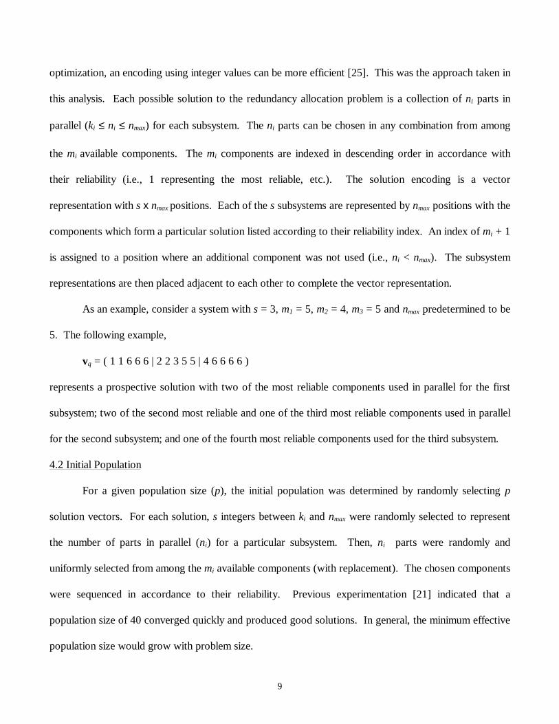
optimization, an encoding using integer values can be more efficient [25]. This was the approach taken in

this analysis. Each possible solution to the redundancy allocation problem is a collection of ni parts in

parallel (ki ≤ ni ≤ nmax) for each subsystem. The ni parts can be chosen in any combination from among

the mi available components. The mi components are indexed in descending order in accordance with

their reliability (i.e., 1 representing the most reliable, etc.). The solution encoding is a vector

representation with s x nmax positions. Each of the s subsystems are represented by nmax positions with the

components which form a particular solution listed according to their reliability index. An index of mi + 1

is assigned to a position where an additional component was not used (i.e., ni < nmax). The subsystem

representations are then placed adjacent to each other to complete the vector representation.

As an example, consider a system with s = 3, m1 = 5, m2 = 4, m3 = 5 and nmax predetermined to be

5. The following example,

vq = ( 1 1 6 6 6 | 2 2 3 5 5 | 4 6 6 6 6 )

represents a prospective solution with two of the most reliable components used in parallel for the first

subsystem; two of the second most reliable and one of the third most reliable components used in parallel

for the second subsystem; and one of the fourth most reliable components used for the third subsystem.

4.2 Initial Population

For a given population size (p), the initial population was determined by randomly selecting p

solution vectors. For each solution, s integers between ki and nmax were randomly selected to represent

the number of parts in parallel (ni) for a particular subsystem. Then, ni parts were randomly and

uniformly selected from among the mi available components (with replacement). The chosen components

were sequenced in accordance to their reliability. Previous experimentation [21] indicated that a

population size of 40 converged quickly and produced good solutions. In general, the minimum effective

population size would grow with problem size.

10

4.3 Objective Function

The problem formulation was to solve the dual of the original problem. The objective function

was therefore the sum of the reliability (Problem P1) or cost (Problem P2) and a dynamic penalty function

determined by the relative degree of infeasibility. It is important to search through the infeasible region,

particularly for highly constrained problems, because the optimal solution can most efficiently be reached

via the infeasible region, and often, good feasible solutions are a product of breeding between a feasible

and an infeasible solution. To provide an efficient search through the infeasible region but to assure that

the final best solution is feasible, a dynamic penalty function based on the squared system reliability deficit

was defined to incrementally increase the penalty for infeasible solutions as the search progresses. The

penalty function used here is based on the research of Smith and Tate [26], and increased monotonically

with the number of generations, g. For Problem P2, the objective function and penalty function, used for

this analysis, are defined as follows. Exact reliability estimates are used for each k-out-of-n:G subsystem

by using equation (1). The formulation for Problem P1 is analogous.

f C Pq i q

i

s

( , ) ( ) ( , )λ λv v= +=

∑ x i1

(3)

4.4 Crossover Breeding Operator

The crossover breeding operator provides a thorough search of areas of the sample space already

demonstrated to produce good solutions. For the GA developed, parents were selected based on the

ordinal ranking of their objective function. A uniform random number, U, between 1 and p was

selected and the solution with the ranking closest to U2 is selected as a parent, following the selection

procedure of Tate and Smith [27]. The crossover operator retained all identical genetic information from

both parents and then randomly selected, with equal probability, from either of the two parents for

components which differed. Because the solution encodings were ranked from most to least reliable,

matches were common. This crossover operator is a variation of the uniform crossover operator which

has been shown [28] to be superior to traditional crossover strategies for analyzing combinatorial

11

problems.

4.5 Mutation Operator

The mutation operator performs random perturbations to selected solutions. A predetermined

number of mutations within a generation is set for each GA trial. Each value within the solution vector

(which was randomly selected to be mutated) was changed with probability equal to the mutation rate. A

mutated component was changed to an index of mi + 1 with 50 % probability and to a randomly chosen

component, from among the mi choices, with 50 % probability.

4.6 Evolution

A survival of the fittest strategy was employed. After crossover breeding, the p best solutions

from among the previous generation and the new child vectors were retained to form the next generation.

The fitness measure was the objective function value. Mutation was then performed after culling inferior

solutions from the population. The best solution within the population was never chosen for mutation to

assure that the optimal solution was never altered via mutation. This is a form of elitist selection [29].

The GA was terminated after a preselected number of generations although the optimal solution was

often reached much earlier.

5. EXAMPLES

The GA was used to analyze two different problems with very good results. First, it was

implemented on the 33 variations of the Fyffe, Hines and Lee problem [8] which were attempted by

Nakagawa and Miyazaki [9] in the form of Problem P1. The cost constraint is 130 and the weight

constraint is varied incrementally from 191 to 159. Because of the stochastic nature of GAs, ten trials

were performed for 1200 generation each and the best solution from among the ten trials was used as the

final solution. The maximum reliability identified by the GA was used to compare its performance to

other algorithms.

12

Considering component mixing, the size of the search space is greater than 7.6 x 1033 from

equation (2). For this problem, 18 children and 22 mutations were produced each generation and the

mutation rate was 0.05. As the weight constraint was incrementally lowered to solve new variations of

the problem, it was found that GA performance improved by increasing the severity of the penalty

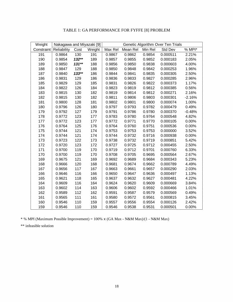
function. Table 1 presents a comparison of the GA results and the corresponding results from the N&M

model. In the table, the percent improvement is the percent that the best feasible solution achieved of the

maximum possible improvement, considering that reliability is bounded by one.

INSERT TABLE 1 HERE

The GA produced feasible final solutions for all 33 problems while the N&M model yielded

feasible solutions for only 30 of the 33. The GA produced a solution with higher reliability than the

N&M or Bulfin and Liu [11] model for 27 of the 33 problems. It was possible to obtain values for

system reliability higher than the previously determined “optimal” solutions because the GA allows

component mixing within a specific subsystem, while the other algorithms do not. In all instances where

there was higher reliability, the improvement was small (< 5%). However, in high reliability applications,

even very small improvements in reliability are often difficult to obtain. In four of the problem variations,

the GA yielded precisely the same solution as the N&M and Bulfin and Liu [11] algorithms, and in 2 of

the 33 problems, the GA produced a solution which was very close, but at a lower reliability.

The second example analyzed is defined by the component choices in Table 2. This problem is of

the form of Problem P2 and the objective is to minimize cost given reliability and weight constraints for a

system designed with two subsystems. For the first subsystem k1 is four, and for the second subsystem,

k2 is two. Cost, weight and reliability component values were selected randomly, however, the

underlying distributions were chosen so that the marginal cost of improved reliability was generally, but

not in every specific case because of random selection, an increasing function with cost. This problem is

13

more difficult than the previous problem in several respects. First, both subsystems are k-out-of-n:G

redundancy with k > 1. Second, for each subsystem, there are ten distinct components choices.

Considering that the mixing of components is allowed, this is a difficult combinatorial problem with over

1.9 x 109 unique solutions (with nmax = 8).

INSERT TABLE 2 HERE

Twenty different GA trials were performed for six different cases of the second example. The

cases differed by changing the reliability and weight constraints as shown in Table 3. For this problem,

15 children and 25 mutations were produced each generation and the mutation rate was 0.25. In each

case the GA was terminated after 1,200 generations, even if the optimal solution had not been reached.

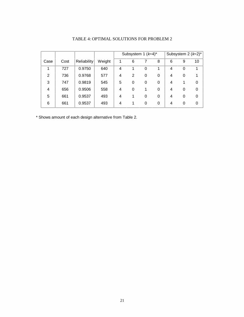
Table 4 presents the optimal solutions for each problem case (obtained by complete enumeration).

INSERT TABLES 3 AND 4 HERE

The results show that the GA consistently converged (i.e., 89%) to the optimal solution.

Additionally, the results yield minimum costs which are between 4.4% and 14.2% better than that which

could be obtained from any of the previously presented integer programming [10, 11, 13-15] or dynamic

programming [8, 9] formulations of the problem. Several of these example cases merit further discussion.

Case 6 is a highly constrained problem. There are only a total of nine feasible solutions (out of 1.9 x

109), all of which require the mixing of components within a subsystem. A competing algorithm which

did not allow mixing of components would not be able to identify any feasible solutions, whereas the GA

identified the optimal solution in 18 out of 20 trials. For case 2, only 11 of 20 trials converged, but the

average solution only differed from the optimal by 0.12% and the worst solution differed by only 0.27%.

Table 3 presents the average number of generations for the GA to converge to its final solution.

Remembering that each generation includes 40 solutions and the search space from equation (2), these

convergence results show the algorithm converges with a percent effort ratio (PER) [12] of less than

14

0.0021% of the search space for a single GA run. This compares to a PER of 3.9% for an integer

programming solution to the redundancy allocation problem using the techniques by Lawler and Bell

[30], and a PER ranging from 0.013% to 10.41% for the algorithm proposed by Misra and Sharma [13].

It should be noted that these integer programming algorithms guarantee convergence to an optimal

solution over a smaller search space while the GA can not guarantee that the optimal solution will be

reached.

15

REFERENCES

[1] C. R. Reeves (ed.), Modern Heuristic Techniques for Combinatorial Problems, 1993, John Wiley &Sons.

[2] M. S. Chern, “On the computational complexity of reliability redundancy allocation in a seriessystem”, Operations Research Letters, vol 11, 1992 Jun, pp 309-315.

[3] F. A. Tillman, C. L. Hwang, W. Kuo, Optimization of System Reliability, 1980; Marcel Dekker.

[4] F. A. Tillman, C. L. Hwang, W. Kuo, “Optimization techniques for system reliability with redundancy- a review”, IEEE Transactions on Reliability, vol R-26, 1977 Aug, pp 148-155.

[5] R. E. Bellman, Dynamic Programming, 1957; Princeton University Press.

[6] R. E. Bellman, E. Dreyfus, “Dynamic programming and reliability of multicomponent devices,Operations Research, vol 6, 1958 Mar-Apr, pp 200-206.

[7] R. E. Bellman, E. Dreyfus, Applied Dynamic Programming,1962; Princeton University Press.

[8] D. E. Fyffe, W. W. Hines, N. K. Lee, “System reliability allocation and a computational algorithm”,IEEE Transactions on Reliability, vol R-17, 1968 Jun, pp 64-69.

[9] Y. Nakagawa, S. Miyazaki, “Surrogate constraints algorithm for reliability optimization problemswith two constraints”, IEEE Transactions on Reliability, vol R-30, 1981 Jun, pp 175-180.

[10] P. M. Ghare, R. E. Taylor, “Optimal redundancy for reliability in series system”, OperationsResearch, vol 17, 1969 Sep, pp 838-847.

[11] R. L. Bulfin, C. Y. Liu, “Optimal allocation of redundant components for large systems”, IEEETransactions on Reliability, vol R-34, 1985 Aug, pp 241-247.

[12] M. Fisher, “The Lagrangian relaxation method for solving integer programming problems”,Management Science, vol 27, 1981 Jan, pp 1-18.

[13] K. B. Misra, U. Sharma, “An efficient algorithm to solve integer programming problems arising insystem reliability design”, IEEE Transactions on Reliability, vol 40, 1991 Apr, pp 81-91.

[14] M. Gen, K. Ida, Y. Tsujimura, C. E. Kim, “Large-scale 0-1 fuzzy goal programming and itsapplication to reliability optimization problem”, Computers and Industrial Engineering, vol 24, 1993,pp 539-549

[15] M. Gen, K. Ida, J. U. Lee, “A computational algorithm for solving 0-1 goal programming with GUBstructures and its application for optimization problems in system reliability”, Electronics andCommunications in Japan, Part 3, vol 73, 1990 Mar, pp 88-96.

[16] F. A. Tillman, C. L. Hwang, W. Kuo, “Determining component reliability and redundancy foroptimum system reliability”, IEEE Transactions on Reliability, vol R-26, 1977 Aug, pp 162-165.

[17] C. L. Hwang, F. A. Tillman, W. Kuo, “Reliability optimization by generalized Lagrangian-functionand reduced-gradient methods”, IEEE Transactions on Reliability, vol R-28, 1979 Oct, pp 316-319.

[18] L. Painton, J. Campbell, “Identification of components to optimize improvements in systemreliability”, Proc. of the SRA PSAM-II Conf. on System-based Methods for the Design and Operationof Technological Systems and Processes, 1994 Mar, 10-15-10-20.

16

[19] L. Painton, J. Campbell, “Genetic algorithms in optimization of system reliability,” IEEETransactions on Reliability, 1995 June, vol. 44, no. 2, pp. 172-178.

[20] K. Ida, M. Gen, T. Yokota, “System reliability optimization with several failure modes by geneticalgorithm”, Proceedings of 16th International Conference on Computers and IndustrialEngineering, 1994 Mar, pp 349-352.

[21] D. W. Coit, A. E. Smith, “Use of a genetic algorithm to optimize a combinatorial reliability designproblem”, Proceedings of the 3rd International Engineering Research Conference, 1994 May, pp467-472.

[22] W. Feller, An Introduction to Probability Theory, 1968; John Wiley & Sons.

[23] J. Holland, Adaptation in Natural and Artificial Systems, 1975; Univ. of Michigan Press.

[24] D. E. Goldberg, Genetic Algorithms in Search, Optimization & Machine Learning, 1989; AddisonWesley.

[25] J. Antonisse, “A new interpretation of schema notation that overturns the binary encodingconstraint”, Proceedings of the 3rd International Conference on Genetic Algorithms, 1989, pp 86-91.

[26] A. E. Smith, D. M. Tate, “Genetic optimization using a penalty function”, Proceedings of the 5thInternational Conference on Genetic Algorithms, 1993, pp 499-505.

[27] D. M. Tate and A. E. Smith, “A genetic approach to the quadratic assignment problem”, Computersand Operations Research, 1994, vol. 22, pp 73-83.

[28] G. Syswerda, “Uniform crossover in genetic algorithms”, Proceedings of the 3rd InternationalConference on Genetic Algorithms, 1989, pp 2-9.

[29] J. J. Grenfenstette, “Optimization of control parameters for genetic algorithms”, IEEE Transationson Systems, Man, and Cybernetics, vol 16, 1986, pp 122-128.

[30] E. L. Lawler, M. D. Bell, “A method for solving discrete optimization problems”, OperationsResearch, vol 14, 1966 Nov-Dec, pp 1098-1112.

17

1

1

1

1

1

1

1

3

1

1

3

7 8

7 8

(a) O ptimal F yffe S olution

(b) A lternative Solu tion

FIGURE 1: ALTERNATIVE SOLUTIONS TO SUBSYSTEMS 7 AND 8

18

TABLE 1: GA PERFORMANCE FOR FYFFE [8] PROBLEM

Weight Nakagawa and Miyazaki [9] Genetic Algorithm Over Ten Trials Constraint Reliability Cost Weight Max Rel Mean Rel Min Rel Std Dev % MPI*

191 0.9864 130 191 0.9867 0.9862 0.9854 0.000511 2.21%190 0.9854 132** 189 0.9857 0.9855 0.9852 0.000183 2.05%189 0.9850 131** 188 0.9856 0.9850 0.9838 0.000603 4.00%188 0.9847 129 188 0.9850 0.9848 0.9842 0.000253 1.96%187 0.9840 133** 186 0.9844 0.9841 0.9835 0.000305 2.50%186 0.9831 129 186 0.9836 0.9833 0.9827 0.000285 2.96%185 0.9829 129 185 0.9831 0.9826 0.9822 0.000373 1.17%184 0.9822 126 184 0.9823 0.9819 0.9812 0.000385 0.56%183 0.9815 130 182 0.9819 0.9814 0.9812 0.000271 2.16%182 0.9815 130 182 0.9811 0.9806 0.9803 0.000301 -2.16%181 0.9800 128 181 0.9802 0.9801 0.9800 0.000074 1.00%180 0.9796 126 180 0.9797 0.9793 0.9782 0.000479 0.49%179 0.9792 127 179 0.9791 0.9786 0.9780 0.000370 -0.48%178 0.9772 123 177 0.9783 0.9780 0.9764 0.000548 4.82%177 0.9772 123 177 0.9772 0.9771 0.9770 0.000105 0.00%176 0.9764 125 176 0.9764 0.9760 0.9751 0.000536 0.00%175 0.9744 121 174 0.9753 0.9753 0.9753 0.000000 3.52%174 0.9744 121 174 0.9744 0.9732 0.9716 0.000938 0.00%173 0.9723 122 173 0.9738 0.9732 0.9719 0.000851 5.42%172 0.9720 123 172 0.9727 0.9725 0.9712 0.000455 2.50%171 0.9700 119 170 0.9719 0.9712 0.9701 0.000760 6.33%170 0.9700 119 170 0.9708 0.9705 0.9695 0.000564 2.67%169 0.9675 121 169 0.9692 0.9689 0.9684 0.000343 5.23%168 0.9666 120 168 0.9681 0.9674 0.9662 0.000789 4.49%167 0.9656 117 167 0.9663 0.9661 0.9657 0.000290 2.03%166 0.9646 116 166 0.9650 0.9647 0.9636 0.000497 1.13%165 0.9621 118 165 0.9637 0.9632 0.9627 0.000481 4.22%164 0.9609 116 164 0.9624 0.9620 0.9609 0.000669 3.84%163 0.9602 114 163 0.9606 0.9602 0.9592 0.000466 1.01%162 0.9589 112 162 0.9591 0.9587 0.9579 0.000569 0.49%161 0.9565 111 161 0.9580 0.9572 0.9561 0.000815 3.45%160 0.9546 110 159 0.9557 0.9556 0.9554 0.000126 2.42%159 0.9546 110 159 0.9546 0.9538 0.9531 0.000501 0.00%

* % MPI (Maximum Possible Improvement) = 100% x (GA Max - N&M Max)/(1 - N&M Max)

** infeasible solution

19

TABLE 2: COMPONENT CHOICES FOR PROBLEM 2

Design Subsystem (i)

Alternative 1 (k=4) 2 (k=2)

(j) R C W R C W

1 0.981 95 52 0.931 137 83

2 0.933 86 94 0.917 132 96

3 0.730 80 32 0.885 127 94

4 0.720 75 92 0.857 122 93

5 0.708 61 41 0.836 100 95

6 0.699 45 33 0.811 59 63

7 0.655 40 98 0.612 54 65

8 0.622 36 96 0.432 41 49

9 0.604 31 83 0.389 36 33

10 0.352 26 66 0.339 30 51

20

TABLE 3: GA PERFORMANCE FOR DIFFERENT CASES OF PROBLEM 2

Problem Description GA Performance Over Twenty Trials

Reliability Weight Global Previous Minimum Average Average Number Number

Case Constraint Constraint Minimum Best* Cost Cost # Gen. Optimal Feasible

1 0.975 650 727 770 727 727.25 988.65 18/20 20/20

2 0.975 600 736 770 736 736.90 570.95 11/20 20/20

3 0.975 550 747 871 747 747.00 662.30 20/20 20/20

4 0.95 600 656 711 656 656.00 309.10 20/20 20/20

5 0.95 550 661 711 661 661.00 268.00 20/20 20/20

6 0.95 500 661 none** 661 680.80 226.85 18/20 20/20

* The lowest minimum cost possible from the N&M [9] and Bulfin and Liu [11] formulations adapted for k-out-of-n:G

** Other algorithms do not produce any feasible solutions

21

TABLE 4: OPTIMAL SOLUTIONS FOR PROBLEM 2

Subsystem 1 (k=4)* Subsystem 2 (k=2)*

Case Cost Reliability Weight 1 6 7 8 6 9 10

1 727 0.9750 640 4 1 0 1 4 0 1

2 736 0.9768 577 4 2 0 0 4 0 1

3 747 0.9819 545 5 0 0 0 4 1 0

4 656 0.9506 558 4 0 1 0 4 0 0

5 661 0.9537 493 4 1 0 0 4 0 0

6 661 0.9537 493 4 1 0 0 4 0 0

* Shows amount of each design alternative from Table 2.

22

AUTHORS

David W. Coit; 1178C Benedum Hall; Department of Industrial Engineering; University of Pittsburgh;

Pittsburgh, PA 15261 USA.

David W. Coit received a BS degree in mechanical engineering from Cornell University in 1980,

an MBA degree from Rensselaer Polytechnic Institute in 1988 and an MS degree in industrial engineering

from the University of Pittsburgh in 1993. He is currently a PhD candidate at the University of

Pittsburgh. From 1980 to 1992, he was a reliability engineer and project manager at IIT Research

Institute, Rome NY where he established reliability programs, analyzed the reliability of engineering

designs and developed statistical models to predict reliability of electronic components for client

companies. His current research involves reliability optimization, stochastic optimization techniques and

industrial applications for artificial neural networks. Mr. Coit is a student member of IEEE, IIE and

INFORMS.

Alice E. Smith; 1031 Benedum Hall; Department of Industrial Engineering; University of Pittsburgh,

Pittsburgh, PA 15261 USA, aesmith@engrng.pitt.edu.

Alice E. Smith is Assistant Professor - Industrial Engineering. After ten years of industrial

experience with Southwestern Bell Corporation, she joined the faculty of the University of Pittsburgh in

1991. Her research interests are in modeling and optimization of complex systems using computational

intelligence techniques, and her research has been sponsored by Lockheed Martin Corporation, the Ben

Franklin Technology Center of Western Pennsylvania, and the National Science Foundation, from which

she was awarded a CAREER grant in 1995. She is an Associate Editor of ORSA Journal on Computing

and Engineering Design and Automation, and a registered Professional Engineer in the state of

Pennsylvania. Dr. Smith is a member of IEEE, ASEE and INFORMS, and a senior member of IIE and

SWE.