A Hybrid Parallel Genetic Algorithm for Reliability

6

A Hybrid Parallel Genetic Algorithm for Reliability Optimization

Ki Tae Kim and Geonwook Jeon Korea National Defense University,

Republic of Korea

1. Introduction

Reliability engineering is known to have been first applied to communication and transportation systems in the late 1940's and early 1950's. Reliability is the probability that an item will perform a required function without failure under stated conditions for a stated period of time. Therefore a system with high reliability can be likened to a system which has a superior quality. Reliability is one of the most important design factors in the successful and effective operation of complex technological systems. As explained by Tzafestas (1980), one of the essential steps in the design of multiple component systems is the problem of using the available resources in the most effective way so as to maximize the system reliability, or so as to minimize the consumption of resources while achieving specific reliability goals. The improvement of system reliability can be accomplished using the following methods: reduction of the system complexity, the allocation highly reliable components, and the allocation of component redundancy alone or combined with high component reliability, and the practice of a planned maintenance and repair schedule. This study deals with reliability optimization that maximizes the system reliability subject to resource constraints.

This study suggests mathematical programming models and a hybrid parallel genetic algorithm (HPGA). The suggested algorithm includes different heuristics such as swap, 2-opt, and interchange (except for reliability allocation problem with component choices (RAPCC)) for an improvement solution. The component structure, reliability, cost, and weight were computed by using HPGA and the experimental results of HPGA were compared with the results of existing meta-heuristics and CPLEX.

2. Literature review

The goal of reliability optimization is to maximize the reliability of a system considering some constraints such as cost, weight, and so on. In general, reliability optimization divides into two categories: the reliability-redundancy allocation problem (RRAP) and the reliability allocation problem with component choices (RAPCC).

2.1 The reliability-redundancy allocation problem (RRAP)

The RRAP is the determination of both optimal component reliability and the number of component redundancy allowing mixed components to maximize the system reliability

www.intechopen.com

Real-World Applications of Genetic Algorithms

128

under cost and weight constraints. It is known as the NP-hard problem suggested by Chern (1992).

A variety of algorithms, as summarized in Tillman et al. (1977), and more recently by Kuo & Prasad (2000), Kuo & Wan (2007), including exact methods, heuristics and meta-heuristics have already been proposed for the RRAP. An exact optimal solution is obtained by exact methods such as cutting plane method (Tillman, 1969), branch-and-bound algorithm (Chern & Jan, 1986; Ghare & Taylor, 1969), dynamic programming (Bellman & Dreyfus, 1958; Fyffe et al., 1968; Nakagawa & Miyazaki, 1981; Yalaoui et al., 2005), and goal programming (Gen et al., 1989). However, as the size of problem gets larger, such methods are difficult to apply to get a solution and require more computational effort. Therefore, heuristics and meta-heuristics are used to find a near-optimal solution in recent research.

The research using heuristics is as follows. Kuo et al. (1987) present a heuristic method based on a branch-and-bound strategy and lagrangian multipliers. Jianping (1996) has developed a method called a bounded heuristic method. You & Chen (2005) proposed an efficient heuristic method. Meta-heuristics such as genetic algorithm (Coit & Smith, 1996; Ida et al., 1994; Painton & Campbell, 1995), tabu search (Kulturel-Konak et al., 2003), ant colony optimization (Liang & Smith, 2004), and immune algorithm (Chen & You, 2005) have been introduced to solve the RRAP.

2.2 The reliability allocation problem with component choices (RAPCC)

The RAPCC is the determination of optimal component reliability to maximize the system

reliability under cost constraint. A problem is formulated as a binary integer programming

model with a nonlinear objective function (Ait-Kadi & Nourelfath, 2001), which is

equivalent to a knapsack problem with multiple-choice constraint, so that it is the NP-hard

problem (Garey & Johnson, 1979). Some algorithms for such knapsack problems with

multiple-choice constraint have been suggested in the literature (Nauss, 1978; Sinha &

Zoltners, 1979; Sung & Lee, 1994).

A variety of algorithms including exact methods, heuristics, and meta-heuristics have

already been proposed for the RAPCC. An exact optimal solution is obtained by branch-

and-bound algorithm (Djerdjour & Rekab, 2001; Sung & Cho, 1999). Meta-heuristics such as

neural network (Nourelfath & Nahas, 2003), simulated annealing (Kim et al., 2004; Kim et

al., 2008), tabu search (Kim et al., 2008), and ant colony optimization (Nahas & Nourelfath,

2005) have been introduced to solve the RAPCC. Also, Kim et al. (2008) solved the large-

scale examples by using a reoptimization procedure with tabu search and simulated

annealing.

3. Mathematical programming models

Notations and decision variables in the mathematical programming model are as follows.

n : the number of subsystems

m : the number of components

i : index for subsystems ( 1,2, ,i n= )

j : index for components ( 1,2, ,j m= )

www.intechopen.com


129

SR : system reliability

iR : reliability of subsystem i

SC : system-level constraint limits for cost

SW : system-level constraint limits for weight

ijr : reliability of component j available for subsystem i

ijc : cost of component j available for subsystem i

ijw : weight of component j available for subsystem i

iu : maximum number of components used in subsystem i

ijx : quantity of component j used in subsystem i (for RRAP)

( )1, if component usedinsubsystem

for RAPCC0, otherwise

= ij

j ix

3.1 Reliability-redundancy allocation problem (RRAP)

This study deals with the reliability-redundancy allocation problem in a series-parallel system as shown in Fig. 1.

Fig. 1. Series-parallel system

The relationship between the system reliability ( SR ) and the reliability of subsystem i ( iR ),

in a series system, is shown in Eq. (1).

1

n

S ii

R R=

= ∏ (1)

The relationship between the reliability of subsystem i ( iR ) and the reliability of

component j available for subsystem i ( ijr ), in a parallel system, is shown in Eq. (2).

1

1 1ij

m x

i ijj

R r=

= − − ∏ (2)

www.intechopen.com


130

Using Eqs. (1) and (2), the mathematical programming model of the RRAP in a series-parallel system is as follows.

Maximize 1 1 1

1 1ijxn n m

S i iji i j

R R r= = =

= = − − ∏ ∏ ∏ (3)

Subject to 1 1

n m

ij ij Si j

c x C= =

⋅ ≤ (4)

1 1

n m

ij ij Si j

w x W= =

⋅ ≤ (5)

1

1m

ij ij

x u=

≤ ≤ , 1,2, ,i n= (6)

0ijx ≥ , 1,2, ,i n= , 1,2, ,j m= , Integer (7)

The objective function is to maximize the system reliability in a series-parallel system. Eqs. (4) and (5) show the resource constraints with cost and weight. Eq. (6) shows the maximum and minimum number of components that can be used for each subsystem. Eq. (7) shows the integer decision variables.

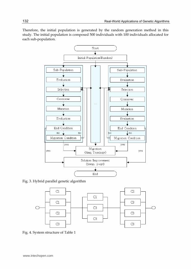
3.2 Reliability allocation problem with component choices (RAPCC)

As shown in Fig. 2, a series system consisting of n subsystems where each subsystem has

several component alternatives which can perform same functions with different

characteristics is considered in this study. The problem is proposed to select the optimal

combination of component alternatives to maximize the system reliability given the cost.

Only one component will be adopted for each subsystem.

Fig. 2. Series system

Using Eq. (1), the mathematical programming model of the RAPCC in a series system is as follows.

Maximize 11

n m

S ij ijji

R r x==

= ⋅ ∏ (8)

Subject to 1 1

n m

ij ij Si j

c x C= =

⋅ ≤ (9)

www.intechopen.com


131

1

1m

ijj

x=

= , 1,2, ,i n= (10)

{ }0,1ijx = , 1,2, ,i n= , 1,2, ,j m= (11)

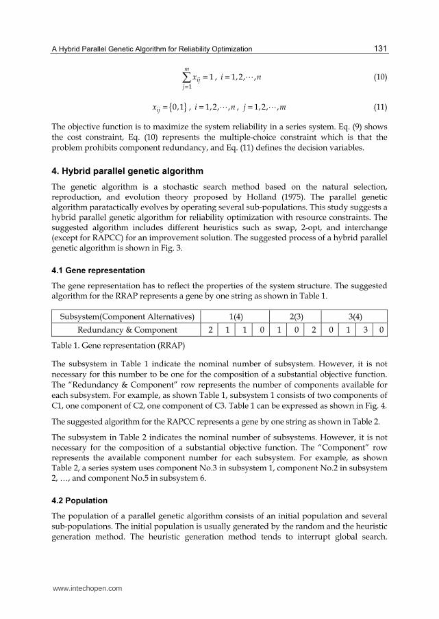
The objective function is to maximize the system reliability in a series system. Eq. (9) shows the cost constraint, Eq. (10) represents the multiple-choice constraint which is that the problem prohibits component redundancy, and Eq. (11) defines the decision variables.

4. Hybrid parallel genetic algorithm

The genetic algorithm is a stochastic search method based on the natural selection, reproduction, and evolution theory proposed by Holland (1975). The parallel genetic algorithm paratactically evolves by operating several sub-populations. This study suggests a hybrid parallel genetic algorithm for reliability optimization with resource constraints. The suggested algorithm includes different heuristics such as swap, 2-opt, and interchange (except for RAPCC) for an improvement solution. The suggested process of a hybrid parallel genetic algorithm is shown in Fig. 3.

4.1 Gene representation

The gene representation has to reflect the properties of the system structure. The suggested algorithm for the RRAP represents a gene by one string as shown in Table 1.

Subsystem(Component Alternatives) 1(4) 2(3) 3(4)

Redundancy & Component 2 1 1 0 1 0 2 0 1 3 0

Table 1. Gene representation (RRAP)

The subsystem in Table 1 indicate the nominal number of subsystem. However, it is not necessary for this number to be one for the composition of a substantial objective function. The “Redundancy & Component” row represents the number of components available for each subsystem. For example, as shown Table 1, subsystem 1 consists of two components of C1, one component of C2, one component of C3. Table 1 can be expressed as shown in Fig. 4.

The suggested algorithm for the RAPCC represents a gene by one string as shown in Table 2.

The subsystem in Table 2 indicates the nominal number of subsystems. However, it is not necessary for the composition of a substantial objective function. The “Component” row represents the available component number for each subsystem. For example, as shown Table 2, a series system uses component No.3 in subsystem 1, component No.2 in subsystem 2, …, and component No.5 in subsystem 6.

4.2 Population

The population of a parallel genetic algorithm consists of an initial population and several sub-populations. The initial population is usually generated by the random and the heuristic generation method. The heuristic generation method tends to interrupt global search.

www.intechopen.com


132

Therefore, the initial population is generated by the random generation method in this study. The initial population is composed 500 individuals with 100 individuals allocated for each sub-population.

Fig. 3. Hybrid parallel genetic algorithm

Fig. 4. System structure of Table 1

www.intechopen.com


133

Subsystem 1 2 3 4 5 6

Component 3 2 4 1 3 5

Table 2. Gene representation (RAPCC)

4.3 Fitness

The fitness function to evaluate the solutions is commonly obtained from the objective function. Penalty functions were used for infeasible solutions by the random generation method in this study. Eqs. (12) and (13) show cost and weight penalty functions, respectively.

1, total cost

1, otherwise

cos

≤=

s

C

C

P

total t

(12)

1, total weight

1, otherwise

≤=

s

W

W

P

total weight

(13)

The multiplication of system reliability and penalty functions related to its cost and weight

(except for RAPCC) were used to calculate the fitness of the solutions in the suggested

algorithm as shown in Eq. (14).

S C Wfitness R P P= ⋅ ⋅ (14)

4.4 Selection

The selection method to choose the pairs of parents is applied by the roulette wheel method in the suggested algorithm. The roulette wheel method is one of the most common

proportionate selection schemes. In this scheme, the probability to select an individual is

proportional to its fitness. It is also stochastically possible for infeasible solutions to survive. The suggested algorithm applies the elitism strategy for the survival of an optimum solution by generation in order to avoid the disappearance of an excellent solution.

4.5 Crossover

The crossover is the main genetic operator. It operates on two individuals at a time and

generates offspring by combining both individuals' features. The crossover operator applies

a uniform crossover in the suggested algorithm as shown in Fig. 5. The steps of the uniform

crossover are as follows.

Step 1. Random numbers were generated for individuals and the individual for crossover was selected by comparing the crossover rate for each individual.

Step 2. The selected individuals were mated between themselves. Step 3. For each bit of the mated individuals was generated a random number of either 0 or 1. Step 4. The two offspring bits were generated through a crossover of the two parents' bits

when the random number associated with those bits was 1.

www.intechopen.com


134

Fig. 5. Uniform crossover

4.6 Mutation

The mutation is a background operator which produces spontaneous random changes in

various individuals. The mutation operator applies the uniform mutation in the suggested

algorithm as shown in Fig. 6. The steps of the uniform mutation are as follows.

Step 1. The mutation bits were selected by comparing a random number with the mutation rate after Generating a random number between 0~1 for all individual bits.

Step 2. The value of the selected bits were substituted with a new value between 0 and the maximum number of components in each subsystem.

Fig. 6. Uniform mutation

4.7 Migration

The migration is an exchange operator to change useful information between neighbor sub-

populations. Periodically, each sub-population sends its best individuals to its neighbors.

When dealing with the migration, the main issues to be considered are migration

parameters such as neighborhood structure, the individuals’ selection for exchanging, sub-

population size, migration period, and migration rate. In the suggested algorithm, the

neighborhood structure uses a ring topology as shown in Fig. 7 and the individuals’

selection for exchanging is determined by the application of the fitness function. Other

migration parameters are shown in Table 3.

www.intechopen.com


135

Fig. 7. Neighborhood structure (ring topology)

Migration parameter Sub-population size Migration period Migration rate

Value 100 50 0.2

Table 3. Migration parameters

4.8 Genetic parameters

The genetic parameters include the population size, crossover rate (Pc), mutation rate (Pm),

and the number of generations. It is hard to find the best parametric values, so the following

parameters were obtained by repeated experiments. The genetic parameters are shown in

Table 4.

Genetic parameter

Population size

Crossover rate(Pc)

Mutation rate(Pm)

The number of generations

Value 500 0.8 0.02 1,000~3,000

Table 4. Genetic parameters

4.9 Improvement solution

The suggested algorithm includes different heuristics such as swap, 2-opt, and interchange

(except for RAPCC) for improvement of the solution. The swap heuristic was used to

exchange each bit which selected two solutions among the five solutions generated by the

parallel genetic algorithm. After applying the swap heuristic, a solution of the parallel

genetic algorithm was selected by using best fitness. In a selected solution, the 2-opt

heuristic performed the exchanging of two bits to enable improvement. The interchange

heuristic was applied to each subsystem to exchanging sequences of bits. Finally, a solution

of a hybrid parallel genetic algorithm was produced using best fitness after the application

of the interchange heuristic.

5. Numerical experiments

5.1 The reliability-redundancy allocation problem (RRAP)

In order to evaluate the performance of the suggested algorithm for the integer nonlinear

RRAP, this study performed experiments on 33 variations of Fyffe et. al. (1968), as suggested

by Nakagawa & Miyazaki (1981). In this problem, the series–parallel system is connected by

www.intechopen.com


136

14 parallel subsystems and each has three or four components of choice. The objective is to

maximize the reliability of the series–parallel system subject to the cost constraint of 130 and

weight constraint ranging from 159 to 190. The maximum number of components is 6 in

each subsystem. The component data for testing problems are listed in Table 5.

Subsystem No.

Component choices

Choice 1 Choice 2 Choice 3 Choice 4

R C W R C W R C W R C W

1 0.90 1 3 0.93 1 4 0.91 2 2 0.95 2 5

2 0.95 2 8 0.94 1 10 0.93 1 9 ＊＊＊

3 0.85 2 7 0.90 3 5 0.87 1 6 0.92 4 4

4 0.83 3 5 0.87 4 6 0.85 5 4 ＊＊＊

5 0.94 2 4 0.93 2 3 0.95 3 5 ＊＊＊

6 0.99 3 5 0.98 3 4 0.97 2 5 0.96 2 4

7 0.91 4 7 0.92 4 8 0.94 5 9 ＊＊＊

8 0.81 3 4 0.90 5 7 0.91 6 6 ＊＊＊

9 0.97 2 8 0.99 3 9 0.96 4 7 0.91 3 8

10 0.83 4 6 0.85 4 5 0.90 5 6 ＊＊＊

11 0.94 3 5 0.95 4 6 0.96 5 6 ＊＊＊

12 0.79 2 4 0.82 3 5 0.85 4 6 0.90 5 7

13 0.98 2 5 0.99 3 5 0.97 2 6 ＊＊＊

14 0.90 4 6 0.92 4 7 0.95 5 6 0.99 6 9

Table 5. Component data for testing problems

To use CPLEX, this study performed additional steps for transforming the integer nonlinear RRAP into an equivalent binary knapsack problem(Bae et al., 2007; Coit, 2003) as shown in Eqs. (15) to (21).

Maximize 1 1

11 0

lni i

i im i im

i im

u un

S ix x ix xi x x

R r y= =

= ⋅ (15)

Subject to 1

11 0 1

i i

i im

i im

u un m

ij ij ix x Si x x j

x c y C= = =

⋅ ⋅ ≤ (16)

1

11 0 1

i i

i im

i im

u un m

ij ij ix x Si x x j

x w y W= = =

⋅ ⋅ ≤ (17)

www.intechopen.com


137

1

1 0

1i i

i im

i im

u u

ix xx x

y=

= , 1,2, ,i n= (18)

1

1m

ij ij

x u=

≤ ≤ , 1,2, ,i n= (19)

0ijx ≥ , 1,2, ,i n= , 1,2, ,j m= , Integer (20)

1

1, if of the th component are used for subsystem

0, otherwisei im

ijix x

x j iy

= (21)

where, ( )1 2

1 1 2ln 1 i i im

i im

x x xix x i i imr q q q= − , ( )1 imim

xximimq r= − , 1,2, ,i n=

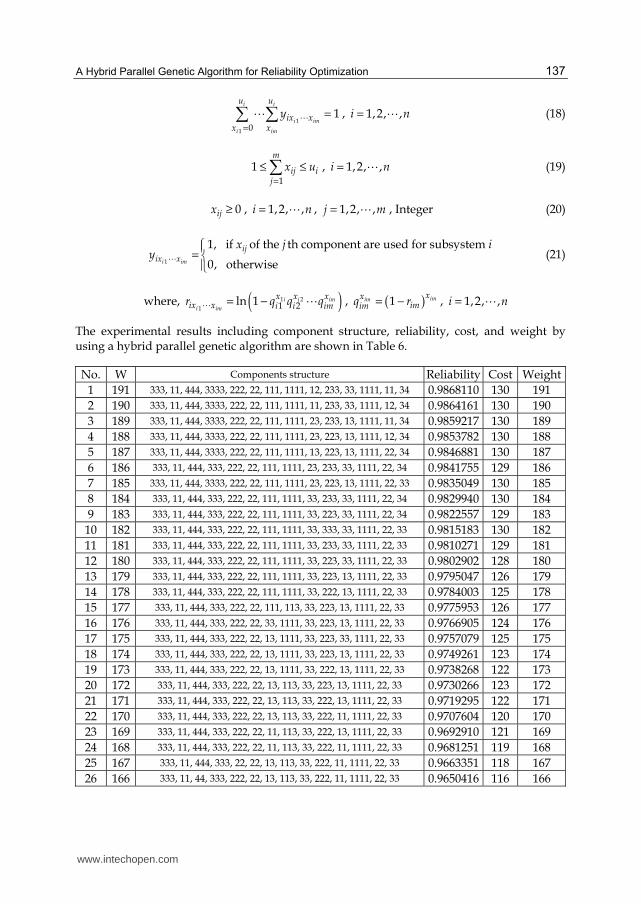
The experimental results including component structure, reliability, cost, and weight by using a hybrid parallel genetic algorithm are shown in Table 6.

No. W Components structure Reliability Cost Weight

1 191 333, 11, 444, 3333, 222, 22, 111, 1111, 12, 233, 33, 1111, 11, 34 0.9868110 130 191

2 190 333, 11, 444, 3333, 222, 22, 111, 1111, 11, 233, 33, 1111, 12, 34 0.9864161 130 190

3 189 333, 11, 444, 3333, 222, 22, 111, 1111, 23, 233, 13, 1111, 11, 34 0.9859217 130 189

4 188 333, 11, 444, 3333, 222, 22, 111, 1111, 23, 223, 13, 1111, 12, 34 0.9853782 130 188

5 187 333, 11, 444, 3333, 222, 22, 111, 1111, 13, 223, 13, 1111, 22, 34 0.9846881 130 187

6 186 333, 11, 444, 333, 222, 22, 111, 1111, 23, 233, 33, 1111, 22, 34 0.9841755 129 186

7 185 333, 11, 444, 3333, 222, 22, 111, 1111, 23, 223, 13, 1111, 22, 33 0.9835049 130 185

8 184 333, 11, 444, 333, 222, 22, 111, 1111, 33, 233, 33, 1111, 22, 34 0.9829940 130 184

9 183 333, 11, 444, 333, 222, 22, 111, 1111, 33, 223, 33, 1111, 22, 34 0.9822557 129 183

10 182 333, 11, 444, 333, 222, 22, 111, 1111, 33, 333, 33, 1111, 22, 33 0.9815183 130 182

11 181 333, 11, 444, 333, 222, 22, 111, 1111, 33, 233, 33, 1111, 22, 33 0.9810271 129 181

12 180 333, 11, 444, 333, 222, 22, 111, 1111, 33, 223, 33, 1111, 22, 33 0.9802902 128 180

13 179 333, 11, 444, 333, 222, 22, 111, 1111, 33, 223, 13, 1111, 22, 33 0.9795047 126 179

14 178 333, 11, 444, 333, 222, 22, 111, 1111, 33, 222, 13, 1111, 22, 33 0.9784003 125 178

15 177 333, 11, 444, 333, 222, 22, 111, 113, 33, 223, 13, 1111, 22, 33 0.9775953 126 177

16 176 333, 11, 444, 333, 222, 22, 33, 1111, 33, 223, 13, 1111, 22, 33 0.9766905 124 176

17 175 333, 11, 444, 333, 222, 22, 13, 1111, 33, 223, 33, 1111, 22, 33 0.9757079 125 175

18 174 333, 11, 444, 333, 222, 22, 13, 1111, 33, 223, 13, 1111, 22, 33 0.9749261 123 174

19 173 333, 11, 444, 333, 222, 22, 13, 1111, 33, 222, 13, 1111, 22, 33 0.9738268 122 173

20 172 333, 11, 444, 333, 222, 22, 13, 113, 33, 223, 13, 1111, 22, 33 0.9730266 123 172

21 171 333, 11, 444, 333, 222, 22, 13, 113, 33, 222, 13, 1111, 22, 33 0.9719295 122 171

22 170 333, 11, 444, 333, 222, 22, 13, 113, 33, 222, 11, 1111, 22, 33 0.9707604 120 170

23 169 333, 11, 444, 333, 222, 22, 11, 113, 33, 222, 13, 1111, 22, 33 0.9692910 121 169

24 168 333, 11, 444, 333, 222, 22, 11, 113, 33, 222, 11, 1111, 22, 33 0.9681251 119 168

25 167 333, 11, 444, 333, 22, 22, 13, 113, 33, 222, 11, 1111, 22, 33 0.9663351 118 167

26 166 333, 11, 44, 333, 222, 22, 13, 113, 33, 222, 11, 1111, 22, 33 0.9650416 116 166

www.intechopen.com


138

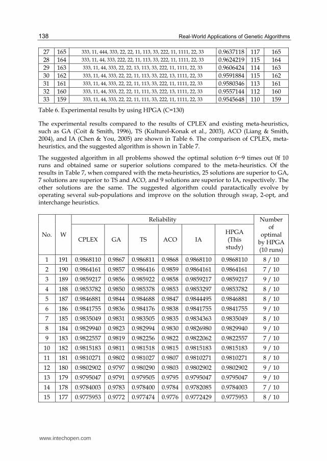
27 165 333, 11, 444, 333, 22, 22, 11, 113, 33, 222, 11, 1111, 22, 33 0.9637118 117 165

28 164 333, 11, 44, 333, 222, 22, 11, 113, 33, 222, 11, 1111, 22, 33 0.9624219 115 164

29 163 333, 11, 44, 333, 22, 22, 13, 113, 33, 222, 11, 1111, 22, 33 0.9606424 114 163

30 162 333, 11, 44, 333, 22, 22, 11, 113, 33, 222, 13, 1111, 22, 33 0.9591884 115 162

31 161 333, 11, 44, 333, 22, 22, 11, 113, 33, 222, 11, 1111, 22, 33 0.9580346 113 161

32 160 333, 11, 44, 333, 22, 22, 11, 111, 33, 222, 13, 1111, 22, 33 0.9557144 112 160

33 159 333, 11, 44, 333, 22, 22, 11, 111, 33, 222, 11, 1111, 22, 33 0.9545648 110 159

Table 6. Experimental results by using HPGA (C=130)

The experimental results compared to the results of CPLEX and existing meta-heuristics, such as GA (Coit & Smith, 1996), TS (Kulturel-Konak et al., 2003), ACO (Liang & Smith, 2004), and IA (Chen & You, 2005) are shown in Table 6. The comparison of CPLEX, meta-heuristics, and the suggested algorithm is shown in Table 7.

The suggested algorithm in all problems showed the optimal solution 6~9 times out 0f 10 runs and obtained same or superior solutions compared to the meta-heuristics. Of the results in Table 7, when compared with the meta-heuristics, 25 solutions are superior to GA, 7 solutions are superior to TS and ACO, and 9 solutions are superior to IA, respectively. The other solutions are the same. The suggested algorithm could paratactically evolve by operating several sub-populations and improve on the solution through swap, 2-opt, and interchange heuristics.

No. W

Reliability Number of

optimal by HPGA (10 runs)

CPLEX GA TS ACO IA HPGA (This

study)

1 191 0.9868110 0.9867 0.986811 0.9868 0.9868110 0.9868110 8 / 10

2 190 0.9864161 0.9857 0.986416 0.9859 0.9864161 0.9864161 7 / 10

3 189 0.9859217 0.9856 0.985922 0.9858 0.9859217 0.9859217 9 / 10

4 188 0.9853782 0.9850 0.985378 0.9853 0.9853297 0.9853782 8 / 10

5 187 0.9846881 0.9844 0.984688 0.9847 0.9844495 0.9846881 8 / 10

6 186 0.9841755 0.9836 0.984176 0.9838 0.9841755 0.9841755 9 / 10

7 185 0.9835049 0.9831 0.983505 0.9835 0.9834363 0.9835049 8 / 10

8 184 0.9829940 0.9823 0.982994 0.9830 0.9826980 0.9829940 9 / 10

9 183 0.9822557 0.9819 0.982256 0.9822 0.9822062 0.9822557 7 / 10

10 182 0.9815183 0.9811 0.981518 0.9815 0.9815183 0.9815183 9 / 10

11 181 0.9810271 0.9802 0.981027 0.9807 0.9810271 0.9810271 8 / 10

12 180 0.9802902 0.9797 0.980290 0.9803 0.9802902 0.9802902 9 / 10

13 179 0.9795047 0.9791 0.979505 0.9795 0.9795047 0.9795047 9 / 10

14 178 0.9784003 0.9783 0.978400 0.9784 0.9782085 0.9784003 7 / 10

15 177 0.9775953 0.9772 0.977474 0.9776 0.9772429 0.9775953 8 / 10

www.intechopen.com


139

16 176 0.9766905 0.9764 0.976690 0.9765 0.9766905 0.9766905 7 / 10

17 175 0.9757079 0.9753 0.975708 0.9757 0.9757079 0.9757079 9 / 10

18 174 0.9749261 0.9744 0.974788 0.9749 0.9746901 0.9749261 6 / 10

19 173 0.9738268 0.9738 0.973827 0.9738 0.9737580 0.9738268 8 / 10

20 172 0.9730266 0.9727 0.973027 0.9730 0.9730266 0.9730266 9 / 10

21 171 0.9719295 0.9719 0.971929 0.9719 0.9719295 0.9719295 7 / 10

22 170 0.9707604 0.9708 0.970760 0.9708 0.9707604 0.9707604 9 / 10

23 169 0.9692910 0.9692 0.969291 0.9693 0.9692910 0.9692910 8 / 10

24 168 0.9681251 0.9681 0.968125 0.9681 0.9681251 0.9681251 8 / 10

25 167 0.9663351 0.9663 0.966335 0.9663 0.9663351 0.9663351 8 / 10

26 166 0.9650416 0.9650 0.965042 0.9650 0.9650416 0.9650416 9 / 10

27 165 0.9637118 0.9637 0.963712 0.9637 0.9637118 0.9637118 7 / 10

28 164 0.9624219 0.9624 0.962422 0.9624 0.9624219 0.9624219 7 / 10

29 163 0.9606424 0.9606 0.959980 0.9606 0.9606424 0.9606424 8 / 10

30 162 0.9591884 0.9591 0.958205 0.9592 0.9591884 0.9591884 6 / 10

31 161 0.9580346 0.9580 0.956922 0.9580 0.9580346 0.9580346 7 / 10

32 160 0.9557144 0.9557 0.955604 0.9557 0.9557144 0.9557144 6 / 10

33 159 0.9545648 0.9546 0.954325 0.9546 0.9545648 0.9545648 8 / 10

Table 7. Comparison of CPLEX, meta-heuristics and HPGA (C=130)

In order to calculate the improvement of reliability for existing studies and the suggested

algorithm, a maximum possible improvement (MPI) was obtained by Eqs. from (22) to (25)

and is shown in Fig. 8.

1( ) 1001

HPGA GA

GA

R RL GA

R

−= ×

− (22)

2( ) 1001

HPGA TS

TS

R RL TS

R

−= ×

− (23)

3( ) 1001

HPGA ACO

ACO

R RL ACO

R

−= ×

− (24)

4( ) 1001

HPGA IA

IA

R RL IA

R

−= ×

− (25)

1( )L GA : MPI(%) of GA results

2( )L TS : MPI(%) of TS results

3( )L ACO : MPI(%) of ACO results

www.intechopen.com


140

4( )L IA : MPI(%) of IA results

HPGAR : system reliability by HPGA

GAR : system reliability by GA

TSR : system reliability by TS

ACOR : system reliability by ACO

IAR : system reliability by IA

Fig. 8. MPI

The suggested algorithm improved system reliability better than existing studies except for TS in the 1st~20th test problems in which the weight was heavy. In addition, HPGA found superior system reliability compared to TS in the 29th~32th test problems in which the weight was light. The other solutions are almost the same.

Through the experiment, this study found that the performance of HPGA is superior to the existing meta-heuristics. In order to evaluate the performance of HPGA in large-scale problems, 5 more problems are presented through connecting the system data of testing problem 1 (C=190, W=191) in series systems. The large-scale problems consist of 28 subsystems (C=260, W=382), 42 subsystems (C=390, W=573), 56 subsystems (C=520, W=764), 70 subsystems (C=650, W=955) in series systems. After 10 runs using HPGA, the results compared with the optimal solution by CPLEX are shown in Table 8.

No. Number of subsystems

C W CPLEX HPGA (10 runs)

Max S.D. Number of optimal

1 14 130 191 0.9868110 0.9868110 0.000021 8 / 10

2 28 260 382 0.9740720 0.9740720 0.000147 6 / 10

3 42 390 573 0.9612374 0.9612374 0.000564 4 / 10

4 56 520 764 0.9488162 0.9488162 0.001095 1 / 10

5 70 650 955 0.9370413 0.9370413 0.001732 1 / 10

Table 8. Experimental results of the large-scale problems

www.intechopen.com


141

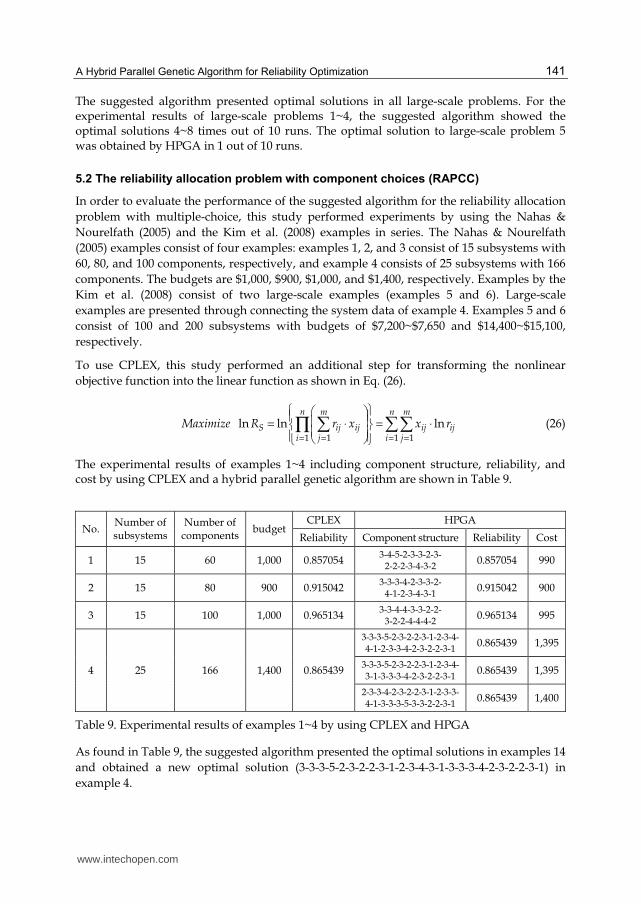
The suggested algorithm presented optimal solutions in all large-scale problems. For the experimental results of large-scale problems 1~4, the suggested algorithm showed the optimal solutions 4~8 times out of 10 runs. The optimal solution to large-scale problem 5 was obtained by HPGA in 1 out of 10 runs.

5.2 The reliability allocation problem with component choices (RAPCC)

In order to evaluate the performance of the suggested algorithm for the reliability allocation

problem with multiple-choice, this study performed experiments by using the Nahas &

Nourelfath (2005) and the Kim et al. (2008) examples in series. The Nahas & Nourelfath

(2005) examples consist of four examples: examples 1, 2, and 3 consist of 15 subsystems with

60, 80, and 100 components, respectively, and example 4 consists of 25 subsystems with 166

components. The budgets are $1,000, $900, $1,000, and $1,400, respectively. Examples by the

Kim et al. (2008) consist of two large-scale examples (examples 5 and 6). Large-scale

examples are presented through connecting the system data of example 4. Examples 5 and 6

consist of 100 and 200 subsystems with budgets of $7,200~$7,650 and $14,400~$15,100,

respectively.

To use CPLEX, this study performed an additional step for transforming the nonlinear

objective function into the linear function as shown in Eq. (26).

Maximize 1 1 11

ln ln lnn m n m

S ij ij ij ijj i ji

R r x x r= = ==

= ⋅ = ⋅ ∏ (26)

The experimental results of examples 1~4 including component structure, reliability, and cost by using CPLEX and a hybrid parallel genetic algorithm are shown in Table 9.

No. Number of subsystems

Number of components

budget CPLEX HPGA

Reliability Component structure Reliability Cost

1 15 60 1,000 0.857054 3-4-5-2-3-3-2-3-

2-2-2-3-4-3-2 0.857054 990

2 15 80 900 0.915042 3-3-3-4-2-3-3-2-

4-1-2-3-4-3-1 0.915042 900

3 15 100 1,000 0.965134 3-3-4-4-3-3-2-2-

3-2-2-4-4-4-2 0.965134 995

4 25 166 1,400 0.865439

3-3-3-5-2-3-2-2-3-1-2-3-4- 4-1-2-3-3-4-2-3-2-2-3-1

0.865439 1,395

3-3-3-5-2-3-2-2-3-1-2-3-4- 3-1-3-3-3-4-2-3-2-2-3-1

0.865439 1,395

2-3-3-4-2-3-2-2-3-1-2-3-3- 4-1-3-3-3-5-3-3-2-2-3-1

0.865439 1,400

Table 9. Experimental results of examples 1~4 by using CPLEX and HPGA

As found in Table 9, the suggested algorithm presented the optimal solutions in examples 14

and obtained a new optimal solution (3-3-3-5-2-3-2-2-3-1-2-3-4-3-1-3-3-3-4-2-3-2-2-3-1) in

example 4.

www.intechopen.com


142

After 10 runs using HPGA in examples 14, the experimental results including maximum, average and standard deviation values were compared with existing meta-heuristics such as ACO (Nahas & Nourelfath, 2005), SA (Kim et al., 2004), and TS (Kim et al., 2008). The comparison of meta-heuristics and the suggested algorithm is shown in Table 10.

No. ACO SA TS

HPGA (This study)

Max Ave. S.D. Max Ave. S.D. Max Ave. S.D. Max Ave. S.D.

1 0.85705 0.85705 0 0.85705 0.85705 0 0.857054 0.857054 0 0.857054 0.857054 0

2 0.91504 0.91504 0 0.91504 0.91504 0 0.915042 0.915042 0 0.915042 0.915042 0

3 0.96512 0.96439 0.00050 0.96513 0.96503 0.00033 0.965134 0.965134 0 0.965134 0.965134 0

4 0.86543 0.86491 0.00038 0.86543 0.86536 0.00025 0.865439 0.865439 0 0.865439 0.865439 0

Table 10. Experimental results of examples 1~4 by using CPLEX and HPGA

The suggested algorithm in examples 14 generated the optimal solutions without standard deviation and showed the same or superior solution compared to meta-heuristics.

In order to evaluate the performance of HPGA in large-scale problems, this study performed experiments by using examples in series as suggested by the Kim et al. (2008). After 10 runs using CPLEX and HPGA in examples 5 and 6, experimental results including maximum, standard deviation values, and maximum possible improvement (MPI) compared with existing meta-heuristics such as simulated annealing, tabu search, and reoptimization procedure by the Kim et al. (2008) are shown in Tables 11 and 12. The MPI was obtained by Eq. (27).

( )

% 100(1 )

Max CPLEXMPI

CPLEX

−= ×

− (27)

Budget CPLEX SA TS HPGA (This Study)

Max S.D. %MPI Max S.D. %MPI Max S.D. %MPI

7,200 0.895758 0.895575 0.001342 -0.1756 0.895758 0.000312 0 0.895758 0.001017 0

7,250 0.900167 0.899438 0.001050 -0.7302 0.899984 0.000305 -0.1833 0.899984 0.000236 -0.1833

7,300 0.904599 0.903866 0.001027 -0.7683 0.904414 0.000390 -0.1939 0.904599 0.000529 0

7,350 0.908866 0.908405 0.001202 -0.5058 0.908866 0.000480 0 0.908866 0.000424 0

7,400 0.913154 0.912601 0.000499 -0.6368 0.913064 0.000337 -0.1036 0.913114 0.000107 -0.0461

7,450 0.917184 0.916815 0.000510 -0.4456 0.917093 0.000494 -0.1099 0.917184 0.000229 0

7,500 0.921141 0.920770 0.000743 -0.4705 0.921141 0.000365 0 0.921141 0.000156 0

7,550 0.925023 0.925023 0.000590 0 0.925023 0.000502 0 0.925023 0.000172 0

7,600 0.929013 0.928269 0.000696 -1.0481 0.929013 0.000445 0 0.929013 0 0

7,650 0.931526 0.931526 0.000388 0 0.931526 0 0 0.931526 0 0

Table 11. Experimental results of example 5 by using CPLEX and HPGA (10 runs)

www.intechopen.com


143

Budget CPLEX TS TS+SA Reoptimization HPGA (This Study)

Max S.D. %MPI Max S.D. %MPI Max S.D. %MPI

14,400 0.802546 0.802218 0.000425 -0.1661 0.802218 0 -0.1661 0.802364 0.000110 -0.0922

14,450 0.806496 0.806167 0.000396 -0.1700 0.806167 0 -0.1700 0.806251 0.000076 -0.1266

14,500 0.810301 0.809890 0.000519 -0.2167 0.809970 0 -0.1745 0.810301 0.000094 0

14,550 0.814290 0.813792 0.000352 -0.2682 0.813792 0 -0.2682 0.813792 0.000182 -0.2682

14,600 0.818299 0.817388 0.000391 -0.5014 0.817798 0.000053 -0.2757 0.817984 0.000003 -0.1734

14,650 0.822160 0.821656 0.000891 -0.2834 0.821656 0 -0.2834 0.822160 0 0

14,700 0.826207 0.824787 0.000709 -0.8171 0.825364 0.000142 -0.4851 0.825774 0.000325 -0.2491

14,750 0.830105 0.829263 0.000815 -0.4956 0.829427 0.000026 -0.3991 0.830105 0.000407 0

14,800 0.833851 0.833428 0.000891 -0.2546 0.833510 0.000026 -0.2052 0.833604 0.000450 -0.1487

14,850 0.837614 0.837448 0.000824 -0.1022 0.837614 0 0 0.837614 0 0

14,900 0.841310 0.840805 0.000786 -0.3182 0.841310 0.000107 0 0.841310 0 0

14,950 0.844856 0.844009 0.000506 -0.5459 0.844856 0.000215 0 0.844856 0 0

15,000 0.848500 0.848332 0.000610 -0.1109 0.848500 0.000027 0 0.848500 0 0

15,050 0.852076 0.851991 0.000722 -0.0575 0.852076 0 0 0.852076 0 0

15,100 0.855751 0.855582 0.000679 -0.1172 0.855751 0 0 0.855751 0 0


As shown in Table 11, the result of SA and TS gave the optimal solution 2 and 6 times out of the 10 cases, respectively. The suggested algorithm found the optimal solution 8 times for the same cases and it showed the same or superior MPI compared to that of SA and TS. As the results in Table 12 show that, when compared with TS and the reoptimization procedure (TS+SA), the suggested algorithm gave the optimal solution 9 times out of the 15 cases and showed the same or superior MPI than TS and the reoptimization procedure (TS+SA). This is because the suggested algorithm could parallelly evolve by operating several sub-populations and improve the solution through swap and 2-opt heuristics.

Throughout the experiment, this study found that performance of HPGA is superior to existing meta-heuristics. This study has generated one more example, example 7, which is presented through connecting the system data of example 4 in series. Example 7 consists of 1,000 subsystems with $90,000$99,000 budgets. After 10 runs using CPLEX and HPGA in example 7, the experimental results including the maximum, standard deviation values, and maximum possible improvement (MPI) are shown in Table 13.

www.intechopen.com


144

Budget CPLEX HPGA

Max S.D. %MPI

90,000 0.831082 0.830757 0.000681 -0.1924

91,000 0.847706 0.846918 0.000594 -0.5174

92,000 0.860003 0.859647 0.000317 -0.2543

93,000 0.871659 0.871516 0.000183 -0.2228

94,000 0.883369 0.883275 0.000262 -0.0806

95,000 0.895226 0.895185 0.000208 -0.0391

96,000 0.904832 0.904832 0.000079 0

97,000 0.913836 0.913791 0.000055 -0.0522

98,000 0.920716 0.920716 0.000016 0

99,000 0.924869 0.924869 0 0


As shown in Table 13, the suggested algorithm presented the optimal solution in 3 times out of 10 cases. While the budget increased, the suggested algorithm found the near-optimal solution.

6. Conclusions

This study suggested mathematical programming models and a hybrid parallel genetic algorithm for reliability optimization with resource constraints. The experimental results compared HPGA with existing meta-heuristics and CPLEX, and evaluated the performance of the suggested algorithm.

The suggested algorithm presented superior solutions to all problems (including large-scale problems) and found that the performance is superior to existing meta-heuristics. This is because the suggested algorithm could paratactically evolve by operating several sub-populations and improve the solution through swap, 2-opt, and interchange (except for RAPCC) heuristics.

The suggested algorithm would be able to be applied to system design with a reliability goal with resource constraints for large scale reliability optimization problems.

7. References

Ait-Kadi, D. & Nourelfath, M. (2001). Availability Optimization of Fault-Tolerant Systems, Proceedings of International Conference on Industrial Engineering Production

Management (IEPM 2001), Quebec, Canada, August, 2001.

Bae, C. O.; Kim, H. G.; Kim, J. H.; Son, J. Y. & Yun, W. Y. (2007). Solving the Redundancy

Allocation Problem with Multiple Component Choice using Metaheuristics,

International Journal of Industrial Engineering, Special Issue, pp.315-323.

Bellman, R. & Dreyfus, S. (1958). Dynamic Programming and the Reliability of

Multicomponent Devices, Operations Research, Vol.6, No.2, pp.200-206.

www.intechopen.com


145

Chern, M. S. (1992). On the Computational Complexity of Reliability Redundancy Allocation

in a Series System, Operations Research Letters, Vol.11, No.5, pp.309-315.

Chern, M. S. & Jan, R. H. (1986). Reliability Optimization Problems with Multiple

Constraints. IEEE Transactions on Reliability, Vol.35, No.4, pp.431-436.

Chen, T. C. & You, P. S. (2005). Immune Algorithms based Approach for Redundant

Reliability Problems with Multiple Component Choices, Computers in Industry,

Vol.56, No.2, pp.195-205.

Coit, D. W. (2003). Maximization of System Reliability with a Choice of Redundancy

Strategies, IIE Transactions, Vol.35, No.6, pp.535-543.

Coit, D. W. & Smith, A. E. (1996). Reliability Optimization of Series-Parallel Systems using a

Genetic Algorithm, IEEE Transactions on Reliability, Vol.45, No.2, pp.254-260.

CPLEX. http://www-947.ibm.com/support/entry/portal.Overview/Software/ WebSphere

/IBM_ILOG_CPLEX

Djerdjour, M. & Rekab, K. (2001). A Branch and Bound Algorithm for Designing Reliable

Systems at a Minimum Cost, Applied Mathematics and Computation, Vol.118, No.2-3,

pp.247-259.

Fyffe, D. E.; Hines, W. W. & Lee, N. K. (1968). System Reliability Allocation and a

Computational Algorithm, Operations Research, Vol.17, No.2, pp.64-69.

Garey, M. R. & Johnson, D. S. (1979). Computers and Intractability: A Guide to the Theory of NP-

Completeness, W. H. Freeman and Company, New York, USA.

Gen, M.; Ida, K.; Sasaki, M. & Lee, J. U. (1989). Algorithm for Solving Large Scale 0-1 Goal

Programming and its Application to Reliability Optimization Problem, Computers

and Industrial Engineering, Vol.17, No.1, pp.525-530.

Ghare, P. M. & Taylor, R. E. (1969). Optimal Redundancy for Reliability in Series System,

Operations Research, Vol.17, No.5, pp.838-847.

Holland, J. H. (1975), Adaption in Natural and Artificial Systems. University of Michigan Press.

Ida, K.; Gen, M. & Yokota, T. (1994). System Reliability Optimization with Several Failure

Modes by Genetic Algorithm, Proceedings of the 16th International Conference on

Computers and Industrial Engineering, Ashikaga, Japan, March, 1994.

Jianping, L. (1996). A Bound Heuristic Algorithm for Solving Reliability Redundancy

Optimization, Microelectronics and Reliability, Vol.3, No.5, pp.335-339.

Kim, H. G.; Bae, C. O.; Kim, J. H. & Son, J. Y. (2008). Solution Methods for Reliability

Optimization Problem of a Series System with Component Choices, Journal of the

Korean Institute of Industrial Engineers, Vol.34, No.1, pp.49-56.

Kim, H. G.; Bae, C. O. & Paik, C. H. (2004). A Simulated Annealing Algorithm for the

Optimal Reliability Design Problem of a Series System with Component Choices, IE

Interfaces, Vol.17, Special Edition, pp.69-78.

Kulturel-Konak, S.; Smith, A. E. & Coit, D. W. (2003). Efficiently Solving the Redundancy

Allocation Problem using Tabu Search, IIE Transactions, Vol.35, No.6, pp.515-526.

Kuo, W.; Lin, H.; Xu, Z. & Zhang, W. (1987). Reliability Optimization with the Lagrange

Multiplier and Branch-and-Bound Technique, IEEE Transactions on Reliability,

Vol.36, No.5, pp.624-630.

Kuo, W. & Prasad, V. R. (2000). An Annotated Overview of System Reliability Optimization,

IEEE Transactions on Reliability, Vol.49, No.2, pp.176-187.

www.intechopen.com


146

Kuo, W. & Wan, R. (2007). Recent Advances in Optimal Reliability Allocation, IEEE

Transactions on systems, man, and cybernetics-Part A: systems and humans, Vol.37,

No.2, pp.143-156.

Liang, Y. C. & Smith, A. E. (2004). An Ant Colony Optimization Algorithm for the

Redundancy Allocation Problem, IEEE Transactions on Reliability, Vol.53, No.3,

pp.417-423.

Nahas, N. & Nourelfath, M. (2005). Ant System for Reliability Optimization of a Series

System with Multiple Choice and Budget Constraints, Reliability Engineering and

System Safety, Vol.87, No.1, pp.1-12.

Nakagawa, Y. & Miyazaki, S. (1981). Surrogate Constraints Algorithm for Reliability

Optimization Problems with Two Constraints, IEEE Transactions on Reliability,

Vol.30, No.2, pp.175-180.

Nauss, R. M. (1978). The 0–1 Knapsack Problem with Multiple Choice Constraints, European

Journal of Operational Research, Vol.2, No.2, pp.121–131.

Nourelfath, M. & Nahas, N. (2003). Quantized Hopfield Networks for Reliability

Optimization, Reliability Engineering and System Safety, Vol.81, No.2, pp.191–196.

Painton, L. & Campbell, J. (1995). Genetic Algorithms in Optimization of System Reliability,

IEEE Transactions on Reliability, Vol.44, No.2, pp.172-178.

Sinha, P. & Zoltners, A. A. (1979). The Multiple Choice Knapsack Problem, Operations

Research, Vol.27, No.3, pp.503–515.

Sung, C. S. & Cho, Y. K. (1999). Branch-and-Bound Redundancy Optimization for a Series

System with Multiple-Choice Constraints, IEEE Transactions on Reliability, Vol.48,

No.2, pp.108-117.

Sung, C. S. & Lee, H. K. (1994). A Branch-and-Bound Approach for Spare Unit Allocation in

a Series System, European Journal of Operational Research, Vol.75, No.1, pp.217–232.

Tillman, F. A. (1969). Optimization by Integer Programming of Constrained Reliability

Problems with Several Modes of Failure, IEEE Transactions on Reliability, Vol.18,

No.2, pp.47-53.

Tillman, F. A.; Hwang, C. L. & Kuo, W. (1977). Optimization Techniques for System

Reliability with Redundancy-a Review, IEEE Transactions on Reliability, Vol.26,

No.3, pp.148-155.

Tzafestas, S. G. (1980). Optimization of System Reliability: A Survey of Problems and

Techniques, International Journal of Systems Science, Vol.11, No.4, pp.455-486.

Yalaoui, A.; Chatelet, E. & Chu, C. (2005). A New Dynamic Programming Method for

Reliability and Redundancy Allocation, IEEE Transactions on Reliability, Vol.54,

No.2, pp.254-261.

You, P. S. & Chen, T. C. (2005). An Efficient Heuristic for Series-Parallel Redundant

Reliability Problems, Computers and Operations Research, Vol.32, No.8, pp.2117-2127.

www.intechopen.com

Real-World Applications of Genetic AlgorithmsEdited by Dr. Olympia Roeva

ISBN 978-953-51-0146-8Hard cover, 376 pagesPublisher InTechPublished online 07, March, 2012Published in print edition March, 2012

InTech EuropeUniversity Campus STeP Ri Slavka Krautzeka 83/A 51000 Rijeka, Croatia Phone: +385 (51) 770 447 Fax: +385 (51) 686 166www.intechopen.com

InTech ChinaUnit 405, Office Block, Hotel Equatorial Shanghai No.65, Yan An Road (West), Shanghai, 200040, China

Phone: +86-21-62489820 Fax: +86-21-62489821

The book addresses some of the most recent issues, with the theoretical and methodological aspects, ofevolutionary multi-objective optimization problems and the various design challenges using different hybridintelligent approaches. Multi-objective optimization has been available for about two decades, and itsapplication in real-world problems is continuously increasing. Furthermore, many applications function moreeffectively using a hybrid systems approach. The book presents hybrid techniques based on Artificial NeuralNetwork, Fuzzy Sets, Automata Theory, other metaheuristic or classical algorithms, etc. The book examinesvarious examples of algorithms in different real-world application domains as graph growing problem, speechsynthesis, traveling salesman problem, scheduling problems, antenna design, genes design, modeling ofchemical and biochemical processes etc.

How to referenceIn order to correctly reference this scholarly work, feel free to copy and paste the following:

Ki Tae Kim and Geonwook Jeon (2012). A Hybrid Parallel Genetic Algorithm for Reliability Optimization, Real-World Applications of Genetic Algorithms, Dr. Olympia Roeva (Ed.), ISBN: 978-953-51-0146-8, InTech,Available from: http://www.intechopen.com/books/real-world-applications-of-genetic-algorithms/a-hybrid-parallel-genetic-algorithm-for-reliability-optimization

© 2012 The Author(s). Licensee IntechOpen. This is an open access articledistributed under the terms of the Creative Commons Attribution 3.0License, which permits unrestricted use, distribution, and reproduction inany medium, provided the original work is properly cited.

http://creativecommons.org/licenses/by/3.0

Documents

A Hybrid Parallel Genetic Algorithm for Reliability