TRA NSPORTATION RESEA RCH RECOR D 1291 315

Reliability Analysis for Wood Bridges

ANDRZEJ s. NOWAK

A probabilistic approach for analysis of wood bridges is discussed . Load and resistance parameters are treated as random variables. The statistical models are derived on the basis of truck surveys, test data, and analysis. The mean maximum 75-year live load is calculated for single- and two-lane bridges. For low-volume roads, the maximum moments can be reduced by about 10 percent. Resistance is considered for timber stringers, glued-laminated (glulam) girders, and stressed decks. A considerable variation of modulus of rupture (MOR) is observed for sawn lumber. The degree of variation of MOR is considerably reduced in case of glulam girders and tressed decks. Reliability is a convenient mea­sure of tructural performance. Reliability indices are caiculated for three structural types. The effect of traffic volume is negligible for timber stringers, but it can be considered for glulam girders and stressed decks.

Wood is an attractive material for bridge construction. It can be used successfully on low-volume roads. Very promising are new structural systems , including glued-laminated (glu­Iam) girders and stressed decks . They allow for the use of low-grade local materials and are suitable for designs and repair or rehabilitation projects. However, there is a need for a rational basis for the development of design criteria.

Traditionally, a considerable variation of mechanical prop­erties such as modulus of rupture (MOR) and modulus of elasticity (MOE) led to low values of the allowable stresses. Introduction of new technologies, including glulam girders and stressed decks, requires a new approach to the design and evaluation of wood structures. Load and resistance parameters are random variables. Therefore , reliability is a convenient measure of the structural performance that also provides a rational basis for comparison between wood and other structural materials.

The parameters involved in the design and evaluation of wood bridges are reviewed and a probabilistic basis for the development of load and resistance factors is developed. The load model is based on the available truck survey data. Resist­ance parameters are derived from test data and simulations. The procedure is formulated for calculation of reliability indices for sawn stringers, glulam girders and stressed decks, as shown in Figure 1.

BRIDGE LOADS

Bridge load components include dead load, live load, dynamic load, environmental loads and others (collision). A combi­nation of the first three components is considered.

University of Michigan, 2370 G. G. Brown Building, Ann Arbor, Mich. 48109.

Dead Load

In case of wood bridges, dead load is usually a small portion of the total load. The major components of dead load, D, are the weight of the structural members and the weight of asphalt (if any). The density of wood, which varies depending on species and moisture, is assumed equal to 60 lb/ft3 for hardwood and 40 lb/ft3 for softwood. Dead load is normally distributed . The statistical parameters of D are presented in Table 1 (J).

Live Load

Live load, L, covers a range of forces produced by vehicles moving on the bridge . The effect of live load depends on many parameters , including span length, truck weight, axle loads, axle configuration, position of the vehicle on the bridge (transverse and longitudinal), number of vehicles on the bridge (multiple presence) , and stiffness of structural members. The maximum live load effect also depends on the time period considered. Bridges are usually designed for an economic life of 50 to 75 years. Shorter periods of time are considered in case of serviceability limit states.

The development of the live load model requires an exten­sive data base, weigh-in-motion (WIM) measurements, or truck surveys. The model described in the following para­graphs is based on the results of the truck survey performed by the Ontario Ministry of Transportation in 1975 (2). About 10,000 heavy trucks were measured (only heavily loaded vehi­cles were included) .

Moments were calculated for various simple spans. The calculations were performed for trucks and axle configura­tions, with about 10 configurations per vehicle. For spans from 10 to 100 ft, the results are shown in Figure 2 on normal probability paper. The vertical scale is the inverse normal probability function . Any distribution represented by a straight line on normal probability paper is a normal function. There­fore , the shape of obtained distributions indicates the type. The moments are divided by the design values, for the HS-20 truck (3).

The maximum 75-year moment can be estimated by extrap­olation. The surveyed trucks represent about 2 weeks' traffic on an Interstate highway. In 75 years, there will be about 1,500 times more vehicles. Let N be the number of trucks and axle configurations. For a 2-week period, N = 100,000, and for 75 years N = 150,000,000. The corresponding prob­ability of occurrence , PN, is equal to the inverse of the number of vehicles, PN = l/N. The corresponding inverse normal distribution, Z , is

Z = <1>- 1 (PN) (1)

where <I> is the standard normal distribution function.

(a) Timber Stringers

Stringers

(b) Glulam Girders

Asphalt

Deck

(c) Stressed Deck

Prestressing Force

FIGURE 1 Wood bridge types considered in this study.

TABLE 1 STATISTICAL PARAMETERS OF DEAD LOAD

It em

Wood Members

Asphalt

Mean-to-Nominal

1. 05

3.5 in

Coefficient of Variation

0.10

0.15

Nowak 317

6

z z- = 5.67

z 5.62

z 5.19

5 :Z 4.89

z 4.42 z

4 40 ft

z 3. 71

0.5 1. 0 1. 5

Truck Moment/AASHTO Moment

FIGURE 2 Distributions of moments on normal probability paper.

Values of time period, T, number of trucks and axle con­figurations, N, and corresponding probability and inverse nor­mal distribution function are presented in Table 2.

The maximum moment is calculated for single- and two­lane bridges. For a single lane, one truck governs for short and medium spans (up to about 100 ft). For two lanes, the maximum effects are obtained for two trucks side-by-side, with perfectly correlated weights . The probability of occur­rence of such an event is about 500 times Jess than occurrence of a single truck. If for a single truck Z = 5.67, then for two perfectly correlated trucks Z = 4.50, which corresponds to the maximum monthly truck.

The mean maximum 75-year moments for a single lane are plotted in Figure 3. For two lanes, the mean maximum moment is obtained for two trucks, one per lane, each about 0.85 of the mean maximum 75-year truck. For comparison, the design AASHTO (3) moments are also shown .

For low-volume roads, the number of trucks is lower. Depending on the actual average daily truck traffic (ADTT), the mean maximum 75-year moments are reduced compared to what is shown in Figure 3. The moment ratios are presented in Table 3. Mhigh is the moment calculated for a busy interstate highway; M10w is the moment for a reduced traffic volume. The corresponding values of Z are also included in the table .

318 TRANSPORTATION RESEARCH RECORD 1291

TABLE 2 VALUES OFT, N, PN, AND Z

Time Period Number Probability Inverse Normal

T

75 years

50 years

5 years

1 year

1 month

2 weeks

1 day

10,00

8, 00'0

6,00

4,00

2,00

N

150,000,000

100,000,000

10,000,000

2,000,000

200,000

100,000

10,000

Moment (kip-ft)

50

z

710 -9 5.67

110 -8 5. 62

110 -7 5 .19

5 10 -7 4.89

5 10 -6 4.42

110 -5 4.26

110 -4 1.71

100 150 200

Span (ft)

FIGURE 3 Mean maximum 75-year moments and AASHTO moments.

Dynamic Load

In the current AASHTO specification (3), there is no impact specified for wood bridges. However, observations indicate that dynamic loads should be considered. Extensive tests ( 4) and analytical simulations (1) provide a basis for the <level-

opment of design provisions for steel and concrete girder bridges. Dynamic load is a function of three parameters: sur­face roughness, truck dynamics, and bridge properties (nat­ural frequency). The calculated mean dynamic load is 0.15mu and mL is the mean maximum 75-year live load, and coeffi­cient of variation is 0.80. However, very little data are avail-

Nowak 319

TABLE 3 MAXIMUM LIVE LOAD FOR LOW-VOLUME ROAD BRIDGES

Traffic Ratio One Lane Two Lanes

(High Volume ADTT/

Low Volume ADTT) z

5.67

10 5.27

50 4. 97

100 4. 83

able for wood bridges. In this study, the mean dynamic load for wood bridges is assumed as O.lOmL with coefficient of variation 0.80.

RESISTANCE

Bridge capacity depends on the resistance of its components and connections. The component resistance, R, is determined mostly by material strength and dimensions. In wood bridges, R depends also on moisture content and load duration. R is a random variable.

In this study, R is considered as a product of the nominal resistance, Rn, and three parameters: strength of material, M; fabrication (dimension) factor, F; and professional analysis factor, P.

(2)

The mean value, mR, of Rand coefficient of variation, VR, are given by the expressions

(3)

(4)

where mM, mF, and mp are the means, and VM, VF, and VP are the coefficients of variation of M, F, and P, respectively.

Sawn Lumber

The variation in material strength and dimensions can be determined from the available test data. Extensive tests were carried out at the University of British Columbia and Western Forest Products Laboratory (5). The analysis of results was provided by Nowak ( 6). Statistical parameters were calculated for the MOR, MOE, dimensions, and correlation between MOR and MOE.

Examples of distribution functions of MOR are shown in Figure 4 for Douglas fir select and Figure 5 for Douglas fir Grades 1 and 2. Nominal dimensions are also indicated. The means and coefficients of variation are presented in Table 4 for Douglas fir (D-F), hemlock fir (H-F), and spruce-pine-fir

Mhigh/Mlow z Mhigh/Mlow

1. 00 4.50 0.85

0.94 3.99 0.80

0.91 3.59 0.79

0.90 3.41 0.78

(S-P-F). The allowable stresses are equal to about 0.25 to 0.35 of the mean MOR (3).

The statistical parameters were also calculated for MOE. The means and coefficients of variation are presented in Table 5. For comparison, the nominal (design) values of MOE vary from 1,600 to 1,800 ksi for D-F, 1,300 to 1,500 ksi for H-F, and 1,400 to 1,800 ksi for southern pine (3).

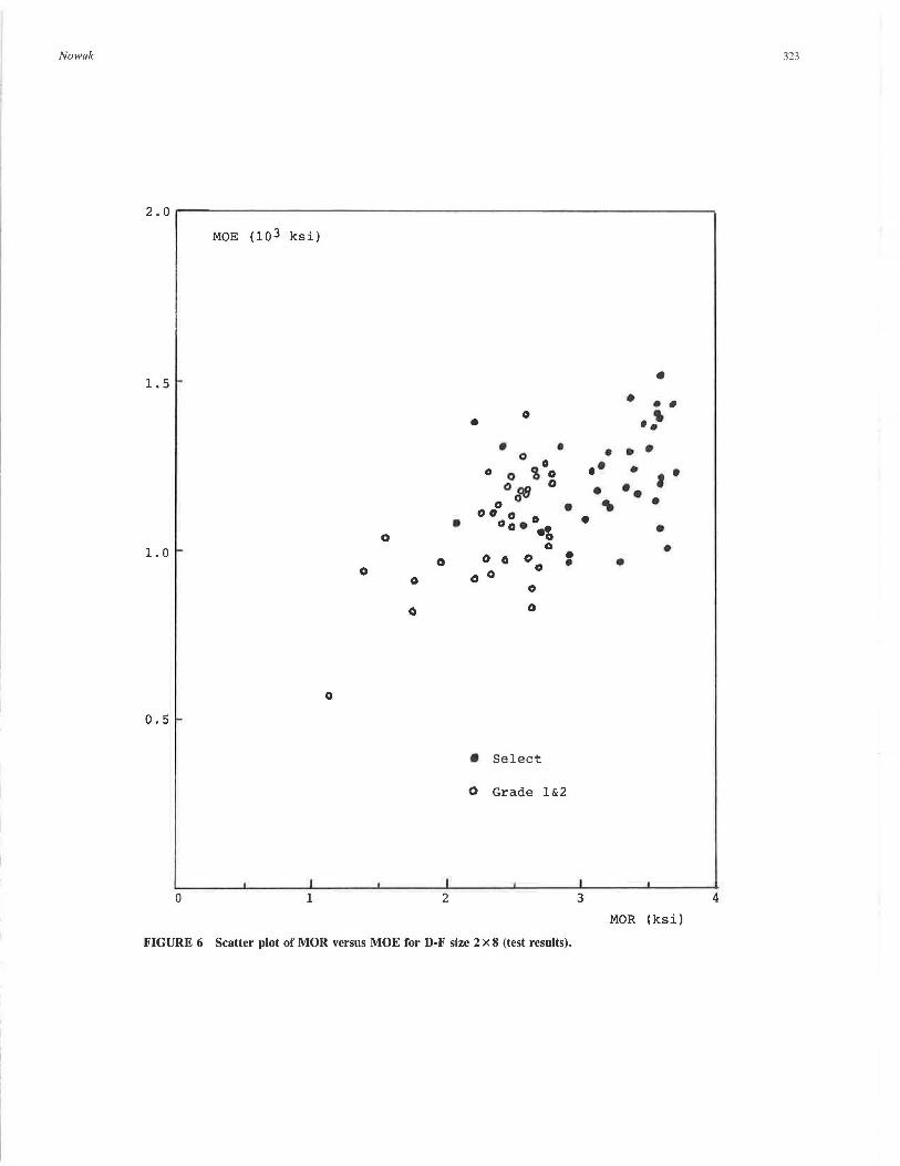
Typical scatter plots of MOR and MOE are shown in Figure 6 for D-F 2 by 8s and in Figure 7 for D-F 3 by 8s. Only a small degree of correlation between MOR and MOE is observed.

Observations of the test data indicate that dimension parameters do not depend on species. The nominal dimension is considered as dressed size (0.5 in. less than commercial size). The ratio of mean-to-normal varies from 0.96 to 1.025 and the coefficient of variation from 0.01 to 0.08.

For the professional analysis factor, it is assumed that mp

= 1.0 and VP = 0.10.

Glulam Girders

The statistical parameters of MOR are derived on the basis oftest data summarized by Ellingwood et al. (7) and presented in Table 6. Allowable stress specified by AASHTO (3) is 2,000 to 2,400 psi.

Stressed Wood

The resistance model is developed on the basis of tests carried out by Sexsmith et al. (8). Sawn timber 2 by 10 was placed in units 1, 2, and 3 ft wide. The units were transversely pre­stressed and loaded to failure. Three species were consid­ered-hemlock fir, white pine, and red pine. The results of tests are plotted on normal probability paper in Figure 8 (8, 9). The vertical scale is the inverse normal distribution function.

Load-carrying capacity of a prestressed unit can be calcu­lated using the system reliability theory. The unit is a system of parallel elements (2 by 10) sharing the load. The system resistance, R,, is a sum of element resistance values, Re. Therefore, the mean of Rs values is

(5)

1

0

-1

-2

-2

Z (Inverse Normal Distribution Function)

1 2 3 4 5 6 7 8

MOR (ksi)

FIGURE 4 Cumulative distribution functions of MOR for D-F select on normal probability scale.

9

2

1

0

-1

-2

-3

z (Inverse Normal Distribution Function)

1 2 3 4 5 6 7

2x4,4x8,6x12

4x6,8x12 6x8

BxlO

8

MOR (ksi)

FIGURE 5 Cumulative distribution functions of MOR for D-F grades 1 and 2 on normal probability scale.

9

TABLE 4 STATISTICAL PARAMETERS OF MOR

Species Size Select Grade 1&2

(in) Mean (psi) cov Mean (psi) cov

D-F 2><4 6800 0.22 5400 0.29

2x6 6050 0.23 4600 0.30

2x8 5500 0.25 4100 0.32

2x10 5200 0.27 3850 0.32

3x8 6200 0.23 4000 0.29

4x6 7250 0.19 5750 0.26

4x8 6800 0.22 5400 0.29

4><17 6050 0.23 1600 0.30

6x8 7800 0 .17 6300 0.24

6x12 6800 0.22 5400 0.29

6x16 6200 0.23 4800 0.29

8x10 7900 0.17 6400 0.23

8x12 7250 0.19 5750 0.26

H-F 2><4 8450 0.26 7000 0.34

2x6 7300 0.29 5450 0.34

2x8 6600 0.30 4750 0.38

2x10 6200 0.31 4350 0.38

3x12 6600 0.30 4800 0.38

S-P-F 2><4 6950 0.32 6200 0.32

2x6 6200 0.32 6500 0.34

2><8 5400 0.30 4800 0.32

2x10 4950 0.27 4500 0.33

TABLES STATISTICAL PARAMETERS OF MOE

Spe cies Select Grade 1&2

Mean (ksi) cov Mean (ksi) cov

D-F 1,500 0.20 1,300 0.21

H-F 1,650 0.18 1,500 0.20

S- P-F 1,500 0.17 1,400 0.21

Nowak

MOE (103 ksi)

1. 5 ...

0 1. 0 ,_

0 0

0

0

0

0. 5 -

I I I I 0 1 2

•

• 0

• 0 0

0 0 'A 0 0 8'8 0

0 00 0 0

00. • •o 0

0 0

0 0

0 0

0

0

• Select

•

•

:

O Grade 1&2

'

FIGURE 6 Scatter plot of MOR versus MOE for D·F size 2 x 8 (test results).

• •• • ' •

I

3

• • •• ··' • •

• • .. ' •

• • •

MOR (ksi)

323

4

2.0

1. 5

1. 0

0.5

FIGURE 7

MOE (103 ksi)

•

0 D

0 0

0

0

• 0

' ' 1 2

•

•

• • • • •

0 0 • • • 0 •

• o. • • oo

00

f)

0

Select

Grade 1&2

' 3

' 4

MOR (ksi)

Scatter plot of MOR versus MOE for D-F size 3 x 8 (test results).

TABLE 6 STATISTICAL PARAMETERS OF MOR FOR GLULAM GIRDERS

Species Size Grade Mean (psi) cov

D-F 8x16 s 1 7070 0.11

8x16 s 2 6240 0.16

Sitka Spruce 8x16 s 2 5040 0.33

w Hem 8x16 s 2 5300 0.20

5

Nowak

2

1

0

-1

z (Inverse Normal Distribution Function)

1 2 3

325

Hern-Fir

1 ft

4 5 6 7 8 9

MOR (ksi)

FIGURE 8 Cumulative distribution function of MOR for stressed wood on normal probability scale.

where mR,; is the mean of R, values for Element i. If all elements have the same distribution of R, values, then

(6)

where n is the number of elements in the system (unit). For independent elements, the variance of the system is

(7)

or

(8)

where sR,, = standard deviation of R, for Element i . The coefficient of variation of Rs is

(9)

From Equations 6 and 8, the coefficient of variation for a prestressed unit is

(10)

The calculated means, mR, , and coefficients of variation, VR,• are compared with the test results in Table 7 (8-10).

RELIABILITY ANALYSIS

The available reliability methods are described by Thoft­Christensen and Baker (11) and by Melchers (12), among others.

Limit states are boundaries between safety and failure. For example, a beam fails if the moment caused by loads, Q, exceeds the moment-carrying capacity, R. The corresponding limit state function, g, can be written

g=R-Q (11)

If g > 0, the structure is safe; otherwise it fails. The prob­ability of failure, PF• is given by

PF = Prob (R - Q < 0) (12)

Let fR and fQ be the probability density functions (PDFs) of R and Q, respectively. Then (R - Q) is also a random variable and it represents the safety margin, as shown in Fig­ure 9. A direct calculation of PF may be difficult, if not impos­sible. Therefore, it is convenient to measure structural safety in terms of a reliability index, (3 , defined as a function of PF•

(13)

where <1>- 1 is the inverse standard normal distribution func-

326 TRANSPORTATION RESEARCH RECORD 1291

TABLE 7 THEORETICAL AND OBSERVED PARAMETERS OF MOR FOR STRESSED UNITS

Unit

width

1

2

3

>­() c Q) ::J 0-Q) .....

ft

ft

ft

Species Mean

Theory/Test

Hem-Fir 0.98

White Pine 0.82

Red Pine 1. 02

Hem-Fir 1. 05

White Pine 0.75

Red Pine 0. 96

Hem-Fir 1. 02

White Pine 0.87

Red Pine 0.97

Coefficient of Variation

Theory Test

0.13 0.16

0.15 0. 15

0.15 0.21

0.09 0.09

0.10 0.07

0.10 0.14

0.09 0.08

0.08 0.08

0.08 0.07

LL R-0, safety margin

0, load effect

2:- Q) ·- ..... = :J ..O=

C'CI C'CI ..0 lL o_ ct 0

I

0

\ R, resistance

I

Moment FIGURE 9 Density functions of R, Q, and R - Q.

tion. Examples of j3's and corresponding P p's are presented in Table 8.

There are various procedures available for calculation of ~ · these procedures vary with regard to accuracy, required input data, and computing costs. If both R and Q are indepen­dent normal random variables, then the reliability index is

~ = mR - m o

( )

l /Z

s~ + s~

(14)

where mR, m 0 are the means and sR, s0 are the standard deviations of R and Q, respectively.

In this study, R is treated as a lognormal random variable and Q is treated as a normal random variable. The reliability index is calculated using a special iterntive procedure (13). A

computer program was developed to facilitate these compu­tations (1).

RELIABILITY INDICES

Reliability indices are calculated for three types of wood bridges: sawn stringers, glulam girders, and stressed decks.

Sawn Stringers

The design equation relates the allowable stress and loads:

Rallowable S = D + L (15)

where D, L are moments of dead load and live load , rcspec-

Nowak

TABLE 8 RELIABILITY INDEX AND PROBABILITY OF FAILURE

Reliability Index

1. 0

2.0

3.0

4. 0

5.0

6.0

Probability of Failure

0.159

0.0228

0.00135

0.0000317

0.000000287

0.000000000987

TABLE 9 RELIABILITY INDICES FOR WOOD BRIDGES

Type Reliability Index

High Volume Road Low Volume Road

Stringers 2.0-2.5 2.0-2.5

Glulam Girders 3.0-4.0 3.5-4.5

Stressed Deck 3.0-4.0 3.5-4.5

tively and Sis elastic section modulus. For given D and L, the required Rauowabte S can be calculated.

The mean resistance is 3 to 4 times larger than Rauowabte S. The coefficient of variation of resistance is high (0.2 to 0.35 in most cases), because of variation in MOR. It dominates the reliability analysis. The reliability index for wood stringers is typically between 2.0 and 2.5. Traffic reduction on low­volume roads does not have any practical impact on the reli­ability level.

The reliability indices are higher (2.5 to 4.0) for structural systems consisting of stringers and the deck (14).

Glulam Girders

The parameters of R and Q in the limit state function are determined using the available statistical data. Mean resis­tance is 2.5 to 3.5 times larger than nominal (design) value. In most cases, the reliability indices are between 3 and 4.

For low-volume roads, the reliability indices are about 0.5 higher than for high-volume road bridges.

Stressed Wood Decks

Calculations are performed for a 1-ft-wide unit. There are no special provisions for stressed wood in the current AASHTO specification (3). Therefore, the nominal resistance is consid­ered as for a nailed deck. The mean-to-nominal R is about 3 to 4 and coefficient of variation is 0.16. The reliability indices are between 3 and 4 in most cases.

327

For low-volume roads, the reliability indices are about 0.5 higher than for high-volume road bridges.

The calculated reliability indices are summarized in Table 9.

CONCLUSIONS

The approach is presented for reliability analysis of wood bridges. Statistical parameters of load and resistance are derived on the basis of truck surveys, test data, and analysis. Safety is measured in terms of the reliability index.

Reliability indices are calculated for three types of wood bridges: timber stringers, glulam girders, and stressed wood decks. The calculations are performed for high and low vol­umes of traffic. The results indicate that, for glulam girders and stressed decks, the current design provisions (3) are overconservative for low-volume road bridges. For timber stringers, because of a high variation of MOR, the volume of traffic does not have any practical effect on the reliability index.

The reliability-based approach can serve as a basis for the development of LRFD provisions for bridge design codes.

REFERENCES

1. A. S. Nowak, Y-K. Hong, and E-S. Hwang. Calculation of Load and Resistance Factors for OHBDC 1990, Report UMCE 90-06. Department of Civil Engineering, University of Michigan, Ann Arbor, 1990.

2. A. C. Agarwal and M. Wolkowicz. Interim Report on 1975 Com­mercial Vehicle Survey. Research and Development Division, Ministry of Transportation, Downsview, Ontario, Canada, 1976.

3. Standard Specifications for Highway Bridges. AASHTO, Wash­ington, D.C., 1989.

4. J. R. Billing. Dynamic Loading and Testing of Bridges in Ontario. Canadian Journal of Civil Engineering, Vol. 11, No. 4, 1984, pp. 833-843.

5. B. Madsen and P. C. Nielsen. In Grade Testing of Beams and Stringers. Department of Civil Engineering, University of British Columbia, Vancouver, Canada, 1978.

6. A. S. Nowak. Modeling Properties of Timber Stringers. Report UMCE 83Rl. Department of Civil Engineering, University of Michigan, Ann Arbor, 1983.

7. B. Ellingwood et al. Development of a Probability Based Criterion for American National Standard A58. NBS Special Publication 577, National Bureau of Standards, Washington, D.C., 1980.

8. R. G. Sexsmith et al. Load Sharing in Vertically Laminated Post­Tensioned Bridge Decking. Technical Report 6, Western Forest Products Laboratory, Vancouver, British Columbia, Canada, 1979.

9. A. S. Nowak and R. J. Taylor. Ultimate Strength of Timber­Deck Bridges. In Transportation Research Record 1053, TRB, National Research Council, Washington, D.C., 1986, pp. 26-30.

10. A. S. Nowak and R. J. Taylor. Reliability-Based Design Criteria for Timber Bridges in Ontario. Canadian Journal of Civil Engi­neering, Vol. 13, 1986, pp. 1-7.

11. P. Thoft-Christensen and M. J. Baker. Structural Reliability The­ory and Its Applications. Springer-Verlag, 1982, p. 267.

12. R. E. Melchers. Structural Reliability Analysis and Prediction. Ellis Horwood Limited, New York, 1987.

13. R. Rackwitz and B. Fiessler. Structural Reliability Under Com­bined Random Load Sequences. Computer and Structure, No. 9, 1978, pp. 484-494.

14. A. S. Nowak and M. K. Boutros. Probabilistic Analysis of Tim­ber Bridge Decks. ASCE Journal of Structural Engineering, Vol. 110, No. 12, 1984, pp. 2939-2954.