Embed Size (px)
Citation preview
Relativistic Quantum Mechanics
Janos Polonyi
University of Strasbourg
(Dated: January 30, 2020)
Contents
I. Relativistic classical dynamics 4
A. Anti-particles 5
B. Energy of an anti-particle 6
C. Space-time inversions and charge conjugation 9
II. Scalar particle 11
A. Heuristic derivation of the Klein-Gordon equation 11
B. First order formalism for scalar particles 13
1. Equation of motion 14
2. Free particle 16
3. Localization 21
4. The birth of relativistic quantum field theory 25
5. Spread of the wave packet 27
C. External field 30
1. One dimensional potential barrier 32
2. Spherical potential well 33
III. Fermions 34
A. Heuristic derivation of Dirac equation 34
B. Spinors 37
1. Non-relativistic spinors 37
2. Projective representations 41
3. Relativistic spinors 43
4. Dirac equation 46
C. Free particles 48
2
1. Plane wave solutions 49
2. Spin density matrix 50
3. Helicity, chirality, Weyl and Majorana fermions 54
D. Non-relativistic limit 56
E. External field 60
1. Klein paradox 60
2. Spherical potential 62
3. Spin precession 66
A. Multi-valued wave functions 67
1. Particle on the circle 67
2. Charged particle in a ring, the Aharonov-Bohm effect 68
3. Dynamics and multi-valued wave functions 70
4. Topological symmetry 71

3
Quantum mechanics is presented on different levels at the regular university lectures, and these
notes are supposed to bridge Quantum Mechanics II, a detailed discussion of the non-relativistic
one- or two-body problems and Quantum Mechanics III, an introduction to second quantization.
The lecturers usually rightly devote this latter to the technical complexity of the subject which
requires indeed time and attention. But this leaves the students somehow loosing the continuity
and the familiarity of the territory as they suddenly find themselves in the midst of formal quantum
fields, Feynman graphs and scattering amplitudes after having trained themselves with calculating
expectation values using down the Earth coordinate and momentum operators.
There are three sources of problems making the modification of the strategy of the usual non-
relativistic Quantum Mechanics necessary when extended over the relativistic regime:
1. The one-particle states are non-local in the space-time. The non-locality in space arises from
the creation of particle-anti partical pairs when a particle is localized at length scale smaller
than its Compton wavelength. The Lorentz-boost of this state spreads such a non-locality
over the time.
2. The anti-particle generates a wrong sign in the formalism which can be transfered from one
equation to another by redefining some quantities but can not be completely eliminated.
3. The Lorentz boosts changes the spacelike hypersurface where the quantum state is defined
by its wave function and the construction of the transformed state requires the solving of a
highly non-trivial dynamical problem. A particular kind of interaction, taking place during
a measurement, leads to the collapse of the state, a non-covariant procedure, and violates
the covariance of the wave function under Lorentz boosts.
The solution of problem 2. is reached in the second quantized formalism of relativistic quantum
field theory by extending the quantum formalism for many-particle systems. That step leads to the
Fock space to represent the states of multi-particle systems where we can abandon the traditional
one-particle wave function. Thus the scalar product is liberated from the constraints, imposed by
the Lorentz transformations in the first quantized formalism and the dangerous minus sign can
be avoided by a suitable defined scalar product in the Fock space. Having disposed of the wave
function problem 3 is not present anymore and the expectation values in the second quantized
formalism, expressed in term of Green functions, are covariant. Naturally the choice of the state
on which the collaps takes place remains an unresolved problem as in the non-relativistic case.
Problem 1 can not be completely eliminated since the pair creation is a physical phenomenon.

4
However it can be formally hidden by redefining the space coordinate when the quantum fields are
introduced. This change restores the locality in time, too.
I believe that more attention should be payed to these issues to justify the profound modification
of the formalism of the traditional non-relativistic Quantum Mechanics when relativistic quantum
effects are discussed and to prepare the students to accept the formalism of relativistic quantum
field theory. These notes are supposed to help to fill up the gap.
I. RELATIVISTIC CLASSICAL DYNAMICS
Special relativity is about the preservation of the laws of classical physical in different coordinate
systems, called inertial reference frames. Rather than checking the fundamental equations one by
one it is required that
1. a free point particle moves with constant speed and
2. the propagation of light takes place with the same velocity, c
in each reference frame. The first condition is used to find the Lorentz transformation,
xµ = Λµνx
ν , (1)
relating the space-time coordinates, xµ = (ct,x), of different reference frames. The classical and
the quantum equations of motion transform in a covariant manner during these transformation.
The second condition is satisfied by requiring that the Lorentz transformations preserve
s2 = t2 − x2 = xµgµνxν . (2)
The family of linear transformations satisfying this conditions,
gµν = Λµ′
νgµ′ν′Λµ′
ν , (3)
defines the Lorentz group.
The motion of a point particle is described by its world-line, xµ(s), s being a parameter which
can be chosen as the invariant length in case of a massive particle. The invariant length, s, is called
proper time since it gives the time shown by a clock, attached to the particle as long as it moves
in the absence of external force.
The importance of condition 2 is the it introduces the same internal velocity parameter in
the dynamics for all particles. This generates two velocity regimes, v/c ∼ 0 and v/c ∼ 1. The
Newtonian mechanics, v/c→ 0, has no internal scale.
5
p x
p
p+ap+p
2
1
t
t
t
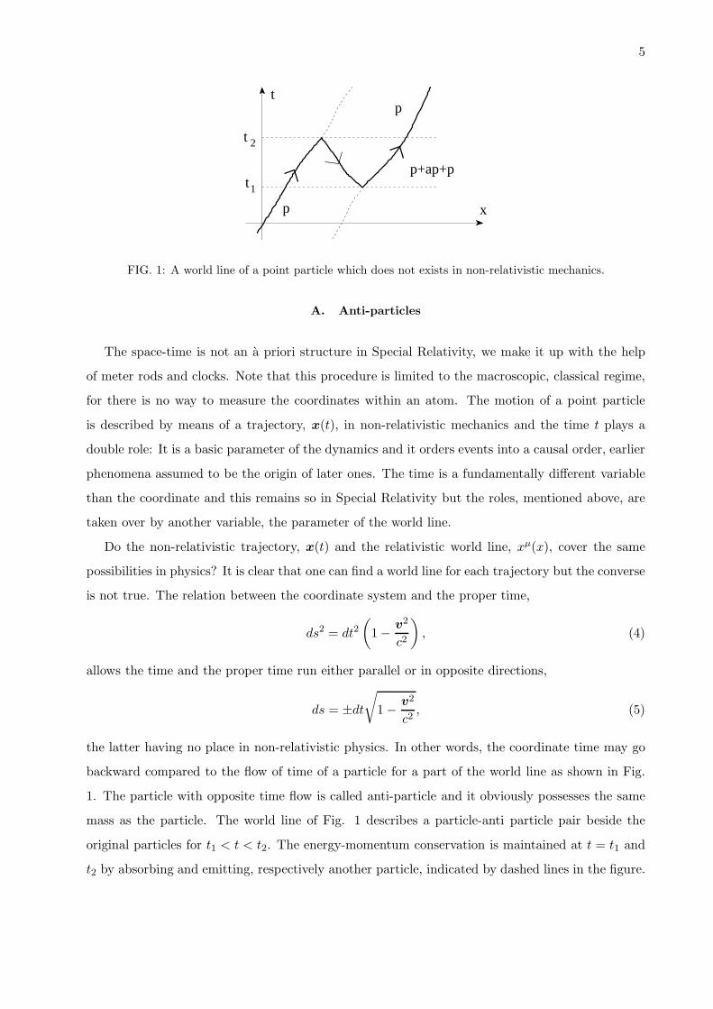
FIG. 1: A world line of a point particle which does not exists in non-relativistic mechanics.
A. Anti-particles
The space-time is not an a priori structure in Special Relativity, we make it up with the help
of meter rods and clocks. Note that this procedure is limited to the macroscopic, classical regime,
for there is no way to measure the coordinates within an atom. The motion of a point particle
is described by means of a trajectory, x(t), in non-relativistic mechanics and the time t plays a
double role: It is a basic parameter of the dynamics and it orders events into a causal order, earlier
phenomena assumed to be the origin of later ones. The time is a fundamentally different variable
than the coordinate and this remains so in Special Relativity but the roles, mentioned above, are
taken over by another variable, the parameter of the world line.
Do the non-relativistic trajectory, x(t) and the relativistic world line, xµ(x), cover the same
possibilities in physics? It is clear that one can find a world line for each trajectory but the converse
is not true. The relation between the coordinate system and the proper time,
ds2 = dt2(
1− v2
c2
)
, (4)
allows the time and the proper time run either parallel or in opposite directions,
ds = ±dt√
1− v2
c2, (5)
the latter having no place in non-relativistic physics. In other words, the coordinate time may go
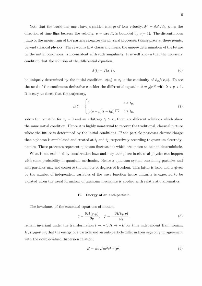
backward compared to the flow of time of a particle for a part of the world line as shown in Fig.
1. The particle with opposite time flow is called anti-particle and it obviously possesses the same
mass as the particle. The world line of Fig. 1 describes a particle-anti particle pair beside the
original particles for t1 < t < t2. The energy-momentum conservation is maintained at t = t1 and
t2 by absorbing and emitting, respectively another particle, indicated by dashed lines in the figure.
6
Note that the world-line must have a sudden change of four velocity, xµ = dxµ/ds, when the
direction of time flips because the velocity, v = dx/dt, is bounded by c(= 1). The discontinuous
jump of the momentum of the particle relegates the physical processes, taking place at these points,
beyond classical physics. The reason is that classical physics, the unique determination of the future
by the initial conditions, is inconsistent with such singularity. It is well known that the necessary
condition that the solution of the differential equation,
x(t) = f(x, t), (6)
be uniquely determined by the initial condition, x(ti) = xi is the continuity of ∂xf(x, t). To see
the need of the continuous derivative consider the differential equation x = g|x|p with 0 < p < 1.
It is easy to check that the trajectory,
x(t) =
0 t < t0,
[g(q − p)(t− t0)]1
1−p t ≥ t0,(7)
solves the equation for xi = 0 and an arbitrary t0 > ti, there are different solutions which share
the same initial condition. Hence it is highly non-trivial to recover the traditional, classical picture
where the future is determined by the initial conditions. If the particle possesses electric charge
then a photon is annihilated and created at t1 and t2, respectively according to quantum electrody-
namics. These processes represent quantum fluctuations which are known to be non-deterministic.
What is not excluded by conservation laws and may take place in classical physics can happen
with some probability in quantum mechanics. Hence a quantum system containing particles and
anti-particles may not conserve the number of degrees of freedom. This latter is fixed and is given
by the number of independent variables of the wave function hence unitarity is expected to be
violated when the usual formalism of quantum mechanics is applied with relativistic kinematics.
B. Energy of an anti-particle
The invariance of the canonical equations of motion,
q =∂H(q, p)
∂p, p = −∂H(q, p)
∂q, (8)
remain invariant under the transformation t → −t, H → −H for time independent Hamiltonian,
H, suggesting that the energy of a particle and an anti-particle differ in their sign only, in agreement
with the double-valued dispersion relation,
E = ±c√
m2c2 + p2, (9)
7
x
x xp ap
t
x
x
x
−
+
t
x
x
x−
+
t
(a) (b) (c)
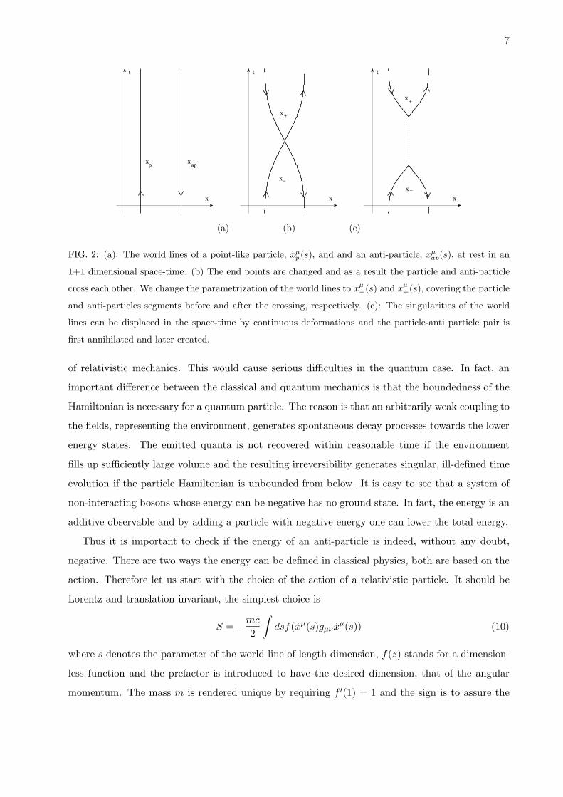
FIG. 2: (a): The world lines of a point-like particle, xµp(s), and and an anti-particle, xµ
ap(s), at rest in an
1+1 dimensional space-time. (b) The end points are changed and as a result the particle and anti-particle
cross each other. We change the parametrization of the world lines to xµ−(s) and xµ
+(s), covering the particle
and anti-particles segments before and after the crossing, respectively. (c): The singularities of the world
lines can be displaced in the space-time by continuous deformations and the particle-anti particle pair is
first annihilated and later created.
of relativistic mechanics. This would cause serious difficulties in the quantum case. In fact, an
important difference between the classical and quantum mechanics is that the boundedness of the
Hamiltonian is necessary for a quantum particle. The reason is that an arbitrarily weak coupling to
the fields, representing the environment, generates spontaneous decay processes towards the lower
energy states. The emitted quanta is not recovered within reasonable time if the environment
fills up sufficiently large volume and the resulting irreversibility generates singular, ill-defined time
evolution if the particle Hamiltonian is unbounded from below. It is easy to see that a system of
non-interacting bosons whose energy can be negative has no ground state. In fact, the energy is an
additive observable and by adding a particle with negative energy one can lower the total energy.
Thus it is important to check if the energy of an anti-particle is indeed, without any doubt,
negative. There are two ways the energy can be defined in classical physics, both are based on the
action. Therefore let us start with the choice of the action of a relativistic particle. It should be
Lorentz and translation invariant, the simplest choice is
S = −mc2
∫
dsf(xµ(s)gµν xµ(s)) (10)
where s denotes the parameter of the world line of length dimension, f(z) stands for a dimension-
less function and the prefactor is introduced to have the desired dimension, that of the angular
momentum. The mass m is rendered unique by requiring f ′(1) = 1 and the sign is to assure the

8
correct non-relativistic limit. The parameter s is not associated with the invariant length at this
stage because such a relation would reduce the number of independent space-time coordinates in
the variational calculus which would be an unwanted complication. Instead, s is identified with
the invariant length after the derivation of the Euler-Lagrange equation,
0 = −mc ddsf ′(x2)xµ
= −mcf ′(x2)xµ − 2mcf ′′(x2)xν xν xµ. (11)
If s is the invariant length then x2 = 1 and the derivative of this identity with respect to s,
xν xν = 0, simplifies the equation of motion to the expected form,
0 = mcxµ. (12)
A possible definition of the energy comes form the canonical energy-momentum,
pµ = − ∂L
∂xµ= mcxµ, (13)
where the minus sign is to have to correct non-relativistic limit for the spatial components of
pµ = (Ec ,−p). The transformation s→ −s change the sign of the energy. Another definition,
Pµ =
∫
d3x√−gTµ0, (14)
is based on the energy-momentum tensor, the source of the gravitational interaction,
Tµν(x) =2√−g
δS
δgµν(x), (15)
where the action is rewriten in terms of a curvlinear coordinate system by the introduction of a
metric tensor gµν(x). This expression arises from the derivation of Einnstein’s equation of General
Relativity by varying the Einstein-Hilbert action with respect to gµν . The action (10) contains the
covariant metrix tensor whose variation can be found by varying the identity δµρ = gµνgνρ,
0 = δgµνgνρ + gµνδgνρ, (16)
yielding
δgµν = −gµρgνσδgρσ . (17)
The action (10), rewritten for general coordinate system reads as
S = −mc2
∫
dxdsδ(4)(x− x(s))f(xµgµν(x)xν) (18)

9
which together with (17) gives the energy-momentum tensor
T µν(x) = mc
∫
dsδ(4)(x− x(s))xµ(s)xν(s). (19)
The corresponding energy-momentum vector,
Pµ = m
∫
dsδ(t− x0(s))xµ(s)x0(s)
= mxµ(s)x0(s)
|x0(s)| , (20)
differs from (13) in a sign, rendering the energy-momentum of a particle and an anti-particle
identical. The lesson is that while the canonical mechanics assigns different sign to the energy of
a particle and an anti-particle the graviational interaction feels the same sign.
We assume now that the particle carries an electric charge and moves in the presence of the
electromagnetic field Aµ(x). The Lagrangian is chosen to be
L = −m2x2 − exµAµ(x), (21)
as the simplest extension of the non-relativistic free particle Lagrangian which changes at most by
a boundary term under gauge transformation, Aµ(x) → Aµ(x) + ∂µα(x), α(x) being an arbitrary
function. We use here the choice f(z) = z in the action (10) and e denotes the charge of the particle.
The Lagrangian (21) looks like that of a charge moving in a magnetic field in 4 dimensional space,
except that the signature of the metric is not definite.
C. Space-time inversions and charge conjugation
The elements of the Lorentz group, L, matrices satisfying (3) can be split into disconnected
sets. By taking the determinant of eq. (3) we have (detΛ)2 = 1. Since the matrix Λ is real its
determinant is real, as well and we must have detΛ = ±1. We define the subsets of the Lorentz
group, L+ and L−, by collecting Lorentz matrices of determinant 1 and −1, respectively. the set
of matrices L+ and L− can not be joined by a continuous path in the Lorentz group because the
determinant is a continuous function of the matrix elements. Thus we have found two disconnected
components of the Lorentz group, L = L+ ∪ L−, of which L+ forms a subgroup.
The matrix element (00) of eq. (3),
1 = (Λ00)
2 −∑
j
(Λ0j)
2, (22)
10
shows that
|Λ00| ≥
√
1 +∑
j
(Λ0j)
2 ≥ 1, (23)
hence elements of the sets L↑ and L↓, containing Lorentz transformation matrices with Λ00 ≥ 1
and Λ00 ≤ −1, respectively give again a partition of the Lorentz group into two disconnected sets,
L = L↑ ∪ L↓, L↑ being a subgroup.
We have finally four disconnected components of the Lorentz group, L↑+ = L+ ∩ L↑, L↓
+ =
L+ ∩ L↓, L↑− = L− ∩ L↑ and L↓
− = L− ∩ L↓. The connected subgroup, L↑+, is called the proper
Lorentz group. The there is a bijective map among the four components, realized by particular
Lorentz transformations, by the space and the time inversions,
P : (t,x)→ (t,−x) (24)
and
T : (t,x)→ (−t,x), (25)
respectively, L↓+ = PTL↑
+, L↑− = PL↑
+ and L↓− = TL↑
+.
Lorentz transformations act on world lines, as well and they bring a physically realizable world
line into another physical one. One can extend the symmetry group of the world lines by a further
discrete transformation, C : s → −s, by exploiting the sign ambiguity, (5), in relating the proper
time and the coordinate time.
Note that the action, constructed by means of the Lagrangian (21) can be made invariant under
the combined transformation CPT by extending the C transformation to the vector potential as
a charge conjugation, C : A → −A. This symmetry is not an accident, it is a rather non-
trivial theorem of relativistic quantum field theory stating that all relativistically invariant, local
Lagrangian are CPT invariant. As a result, the classical Lagrangian, derived from a local quantum
theory should respect this symmetry, as well.
It is advantageous introduce the parity of the discrete transformations, P : f(x, x) →f(Px, P x) = πff(x, x), T : f(x, x)→ f(Tx, T x) = τff(x, x), C : f(x, x)→ f(x,−, x) = γff(x, x),
eg. πt = −πx = 1, −τt = τx = 1 and γxµt = −γxµ = 1. Since any function f(z) can be written as
a sum of an even and an odd part,
f(z) =f(z) + f(−z)
2+f(z)− f(−z)
2, (26)

11
these parities assume the values ±1, in agreement with the relations
P 2 = T 2 = C2 = 11 (27)
in classical physics.
These equations are not necessarily valid in relativistic quantum mechanics, as shown in Ap-
pendix A. The point is the existence of the spin, a relativistic effect. The coordinate space of a
non-relativistic, spinless particle is R3, a connected space. The spin makes it necessary to follow
rotations, as well, and to extend the kinematical space over rotations. We shall see that the rota-
tional group is multiply-connected, a feature of the kinematical space which leads to multi-valued
wave functions. The relative phase between the Rieman-sheets of the wave function introduces
new quantum numbers, changing the parities.
II. SCALAR PARTICLE
The relativistic generalization of the Schrodinger equation for a free particle,
i~∂tψ(x, t) = −~2
2m∆ψ(x, t), (28)
should have the same order of derivative in time and space directions. This can be achieved in two
different manners, both have either first or second order derivatives. The former and the latter
equation, describe fermions and bosons, respectively.
A. Heuristic derivation of the Klein-Gordon equation
The heuristic argument to construct a second order equation of motion is based on the gener-
alization of the three-momentum to
pµ =
(
E
c,−p
)
= i~∂µ = i~(∂0,∇), pµ =
(
E
c,p
)
= i~∂µ = i~(∂0,−∇). (29)
The mass shell condition,
p2 = m2c2x2 = m2c2, (30)
leads to the Klein-Gordon equation
(
�+m2c2
~2
)
φ(x) = 0 (31)
12
as an equation of motion. The parameter ~/mc = λC , the Compton wavelength, is the intrinsic
length scale of a massive particle. Most of the equations below are given in units ~ = c = 1 for
simplicity. The generalization for a charged particle in the presence of an electromagnetic field
Aµ(x), pµ → pµ − q
cAµ is obtained by the help of the covariant derivative ∂µ → ∂µ + i q
~cAµ = Dµ.
Special care is neede to set the value of q, it stands for the charge of the field the covariant
derivative is acting upon. Since the electric charge is defined as the Noether charge, corresponding
to phase rotation, φ(x)→ e−i q~c
αφ(x) the fields φ(x) and φ∗(x) have opposite electric charge, e and
−e, respectively and Dµφ = ∂µφ + i e~cAµφ and Dµφ
∗ = ∂µφ − i e~cAµφ = (Dµφ)
∗. Further useful
properties of the covariant derivative is that it satisfies Leibnitz’s rule, Dφχ = (Dφ)χ+ φDχ, and
therefore allows partial integration. The generalization of (31) for vector potential reads as
(
DµDµ +
m2c2
~2
)
φ(x) = 0. (32)
The Klein-Gordon equation can be considered as the Euler-Lagrange equation for a complex
scalar field φ(x) when the action
S[φ] =
∫
dtd3xL(φ, φ∗,Dµφ,Dµφ∗), (33)
defined by the Lagrangian
L = (Dµφ)∗Dµφ−m2φ∗φ (34)
is used. The Lagrangian is invariant under a continuous symmetry transformation, φ(x)→ eiθφ(x),
and the corresponding conserved Noether-current is
jµ =i
2m(φ∗Dµφ− (Dµφ)
∗φ) =i
2mφ∗←→∂µφ−
e
mcφ∗φAµ, (35)
where the derivative←→∂µ is defined as
f←→∂µg = g∂µg − ∂µgf. (36)
It is the relativistic generalization of the non-relativistic probability current
jµ =
(
ψ∗ψ,1
2im[ψ∗Dψ − (Dψ)∗ψ]
)
=
(
ψ∗ψ,1
2im(ψ∗
∇ψ −∇ψ∗ψ) +e
mcψ∗ψA
)
(37)
of the Schrodinger equation. The O (A) terms in (35)-(37) represent the paramagnetic contribution
to the electric current.
The plane-wave solutions are
φ(x) = e∓ipµxµ
(38)
13
where p0 = ωp with
ωp =√
m2 + p2. (39)
The sign - or + corresponds to positive energy (particle) or negative energy (anti-particle) plane
waves, respectively. The current (35) assumes the form
jµ = ±pµ
m(40)
for a plane wave. The negative energy plane wave represents anti-particles and the form (38) of
the wave function suggests that the energy-momentum pµ is the canonical one, corresponding to
(13).
The Klein-Gordon equation leads to a number of paradoxes of which we mention two only:
1. States with negative energy: The energy of a free particle, defined by the eigenvalue of i∂0 is
not definite. The appearance of negative energy one-particle states poses a serious problem
in quantum mechanics. In fact, the energy of a system of several free bosons can be lowered
without bound in this case and there is no ground state anymore.
2. No probabilistic interpretation: The density ρ of the Klein-Gordon current, (35) jµ = (ρ, j),
is the time component of a four vector rather than a scalar as in non-relativistic quantum
mechanics. It can not be interpreted as probability density because signρ may change during
Lorentz transformation.
Note that these problems are not independent, both of them arise from the same minus sign in the
exponent of the plane wave (38), the existence of anti-particles.
B. First order formalism for scalar particles
The appearence of the anti-particle, the source of the sign problems, mentioned above, can
easily be traced back to the increase of the order of the equation of motion in the time derivative.
The point is that the unique solution of a second order differential equation, (32), needs two
initial conditions, for instance φ(ti,x) and ∂0φ(ti,x). This is an important change with respect to
non-relativistic quantum mechanics, suggesting the presence of two particles, one for each initial
condition function, in the state, represented by φ(t,x). It is natural to identify the second particle
with the anti-particle partner of the original particle. In other words, the wave function,
φ(t,x) =
∫
dω
2πe−iωtφ(ω,x), (41)
14
is a linear superposition of the particle and anti-particle,
φ±(t,x) = Λ±φ(t,x) =
∫
dt′Λ±(t− t′)φ(t′,x) (42)
where the projectors
Λ±(t− t′) = ±∫ ±∞
0
dω
2πe−iω(t−t′∓iǫ)
= − i
2π(t− t′ ∓ iǫ) , (43)
separate the positive and negative frequency components therefore have to act on the time variable.
Owing to the unconstrained integration over t′ in eq. (42) the separation of the particle and
the anti-particle content of the wave function φ(t,x) is possible after infinitely long observation
time. In fact, the energy-time uncertainty principle is due to the non-local nature of the Fourier
transformation. This represents an important difference between the relativistic and the non-
relativistic quantum mechanics, namely the separation of the two relativistic particles can not be
done locally in time. The equation of motion can be used to make the separation locally, by relating
time- and space-dependence for free particles. This solves the problem for free particles but any
change in the equation of motion induces a mixing of the states, defined for the free particles .
This is the way we understand the creation particle-anti particle pairs by external fields, examples
being the electron-positron emission by strong electromagnetic field and the Hawking radiation,
stemming from the gravitational horizon.
The presence of two particles in a state, defined by a single wave function leads to serious
complications and problems in the usual setting of quantum mechanics whose satisfactory solution
requires the formalism of quentum field theory.
1. Equation of motion
To preserve the simple, local nature of the equation of motion in time we separate the two
particles an approximate manner by the introduction of a two-dimensional Klein-Gordon spinor
wave function,
χ+
χ−
=1
2
φ+ im∂0φ
φ− im∂0φ
. (44)
A particle (anti-particle) in rest resides completely in χ1 (χ2) and a slow moving particle (anti-
particle) should have small χ2 (χ1) component. The redoubling of the components of the wave
15
functions halves the order of the differential equation and allows us to write Klein-Gordon equation
as
i∂0
χ+
χ−
=1
2
i∂0φ+ (m− 1m∇
2)φ
i∂0φ+ ( 1m∇
2 −m)φ
. (45)
The relations χ+ + χ− = φ, χ+ − χ− = im∂0φ lead to further simplification,
i∂0
χ+
χ−
=1
2
m(χ+ − χ−) + (m− 1m∇
2)(χ+ + χ−)
m(χ+ − χ−) + ( 1m∇
2 −m)(χ+ + χ−)
, (46)
which can be written as
i∂0χ = Hχ (47)
with the Hamiltonian
H = −∇2
2m(σ3 + iσ2) +mσ3. (48)
The last term on the right hand side sets different rest mass energy for the two components and
the first term adds the kinetic energy. The spectrum of the Hamiltonian is E = ±ωp and the
eigenstate can be identified by the particle and anti-particle states.
Hermiticity The operator H is non-Hermitian, H† 6= H and as a result its eigenvectors,
corresponding to particle and anti-particle are not orthogonal and the unstable. Such a mixing
of the particle and anti-particle state is non-physical and we should restore Hermiticity. This is
achieved by modifying the scalar product by the help of a ”metric operator”, g, 〈ψ|φ〉 → 〈ψ|g|φ〉.This is formally equivalent with the generalization of each vector |ψ〉 to a ”covariant” and a
”contravariant” version, the bra and the ket, respectively. The usual Hermitian conjugation which
maps the ket |ψ〉 into the bra |ψ〉 → |ψ〉† = 〈ψ| is replaced by the bra generated by the Klein-
Gordon conjugation, |ψ〉 → 〈ψ| = 〈ψ|g yielding the scalar product 〈ψ|φ〉 = 〈ψ|g|φ〉. The equation
〈φ|A†|ψ〉 = 〈ψ|A|φ〉∗ defining the matrix elements of the usual Hermitian conjugate A† of an
operator A, is now replaced by 〈φ|A|ψ〉 = 〈ψ|A|φ〉∗ written as 〈φ|gA|ψ〉 = 〈ψ|gA|φ〉∗. Hence we
have gA = (gA)†, yielding the Klein-Gordon conjugate operator, A = g−1A†g†. We shall use
g = σ3 which leads to the matrix elements
〈χ|A|χ′〉 =∫
d3xχ(x)Aχ′(x), (49)
and the Klein-Gordon conjugate of wave functions and operators, χ = χ†σ3 and A→ σ3A†σ3 = A,
respectively. It is easy to check that the Hamiltonian is now Hermitean, H = H.

16
The modification of the Hermitian conjugation and with it the scalar product influences the
physical content, the definition of the expectation values. We are forced to make this momentous
step to assure the orthogonality and the stability of the particle and anti-particle eigenstates of H.
But this comes with a high price: the scalar product becomes indefinite owing to the non-definite
eigenvalues of σ3. In fact, the naive scalar product for the Klein-Gordon wave function,
〈φ|φ′〉 =∫
d3xφ∗(t,x)φ′(t,x), (50)
is now replaced by
〈χ|χ′〉 =∫
d3xχ(t,x)χ′(t,x) =i
2m
∫
d3xφ∗(x)←→∂0 φ
′(x), (51)
in particularly the norm of a Klein-Gordon spinor χ is given by the non-definite Noether charge,
〈χ|χ〉 =∫
d3xj0(t,x). (52)
The result allows us to keep an important feature of the non-relativistic quantum mechanics,
namely that the norm of a state is the space integral of the probability distribution.
Lagrangian The equation of motion (47) can be obtained from the Lagrangian
L =i
2χ∂0χ−
i
2∂0χχ− χHχ. (53)
In fact, the Euler-Lagrange equation, corresponding to the variation of χ is (47) and the variation
of χ yields
i∂0χ = −χH. (54)
Due to H = H this equation of motion is equivalent with eq. (47).
2. Free particle
Plane wave: Let us look for the plane wave solution with positive and negative energy,
χ(x) = upe−ipx, (55)
and
χ(x) = vpeipx. (56)
The mass-shell condition, p2 = m2, requires p0 = ωp and the vectors u and v satisfy the equation
ωpup = Hpup,
17
−ωpvp = Hpvp, (57)
where the Hamiltonian, acting in a given two dimensional momentum subspace is
Hp =p2
2m(σ3 + iσ2) +mσ3. (58)
We shall use the eigenvectors
up =1
2√mωp
m+ ωp
m− ωp
= u−p,
vp =1
2√mωp
m− ωp
m+ ωp
= v−p, (59)
which are orthogonal,
upvp = vpup = 0, (60)
and normalized,
upup = −vpvp = 1. (61)
Wave function: The general solution of the equation of motion (47) can be written as a
Fourier integral,
χ(x) =
∫
p
[apupe−ipx + b∗pvpe
ipx]|p0=ωp, (62)
using the integral measure
∫
p
=
∫
d3p
(2π)3, (63)
and the scalar field, corresponding to this solution, is
φ(x) =
∫
p
√
m
ωp[ape
−ipx + b∗peipx]|p0=ωp
. (64)
The plane waves of the Fourier decomposition of the general solution are always on mass hell,
p0 = ωp. The negative energy component, describing the anti-particle content has the three-
momentum with the wrong sign. This sign problem can be avoided by interpreting the coefficient
function as the complex conjugate of the anti-particle wave function,
ap =i
2√mωp
∫
x
eipx←→∂0 φ(x),
a∗p = − i
2√mωp
∫
x
e−ipx←→∂0φ∗(x),

18
b∗p = − i
2√mωp
∫
x
e−ipx←→∂0φ(x),
bp =i
2√mωp
∫
x
eipx←→∂0 φ
∗(x).
(65)
Note the unusual way both the particle and the anti-particle states are unified within the Klein-
Gordon wave function: φ(x) contains the wave function of the particle and the complex conjugate
of the wave function of the anti-particle. The complex conjugation amounts to the flipping of the
direction of the time, in agreement with the earlier remark that the time runs in the opposite
direction for anti-particles. The wave function, satisfying the second order Klein-Gordon equation
may be real, φ∗(x) = φ(x), and the anti-particle of a neutral particle is identical with the particle.
Non-relativistic limit: The non-relativistic limit for the particle and the anti-particle com-
ponents of the scalar field φ(x) can be found by taking “the square root of the Klein-Gordon
equation”,
i∂0φ(±)(x) = ±
√
m2 −∆φ(±)(x) (66)
yielding
i∂0φ(±)(x) =
[
m− ∆
2m+O
(
(
∆
m
)2)]
φ(±)(x), (67)
and reproduces Schrodinger’s equation in the leading order in p2/m2. The non-relativistic limit for
the Klein-Gordon spinor cam be found by noting that χ2 is suppressed for slow moving particle.
This suggests the strategy to eliminate χ2 by its equation of motion which reduces to an algebraic
calcuation in momentum space. We assume a plane wave, χ(x) = e−ipxηp, satisfying
p0
η1
η2
=1
2
m(η1 − η2) + (m+ 1mp2)(η1 + η2)
m(η1 − η2)− (m+ 1mp2)(η1 + η2)
, (68)
and use its second component to eliminate η2,
η2 = −1mp2
2p0 + 2m+ 1mp2
η1. (69)
the resulting effective equation of motion for χ1,
2p0η1 = m(η1 − η2) + (m+1
mp2)(η1 + η2)
=
(
2m+1
mp2 − ( 1
mp2)2
2p0 + 2m+ 1mp2
)
η1, (70)

19
yields the spectrum, p0 = m+ ǫ,
ǫ =p2
2m− ( 1
mp2)2
8m+ 4ǫ+ 2p2
m
≈ p2
2m− (p2)2
8m2. (71)
However the equations of motion (66) and (70) are not very useful because they are highly non-local
in three space.
Projector: The simplest separation of the particle or anti-particle modes is achieved by using
the projection operator,
Λ±,p =
up ⊗ up
−vp ⊗ vp= ± 1
4mωp
(m± ωp)2 p2
−p2 −(m∓ ωp)2
. (72)
The projection operator in coordinate space,
Λ±(x,y) =
∫
p
eip(x−y)−|p|ǫΛ±,p, (73)
suffers of a singularity as x − y → 0. The fast oscillating contribution of the Fourier integral is
suppressed in any application of the projector operator on states with finite length scale according
to the Riemann-Lebesbgue lemma, to be taken into account by the introduction of a regulator, the
infinitesimal parameter ǫ. The asymptotic behavior
Λ±,p =
± |p|4m(σ3 + iσ2) |p| ≫ m,
12(11± σ3) |p| ≪ m,
(74)
shows that the low momentum, |p| ≪ m, particle and the anti-particle amplitude resides mainly in
the upper and the lower component of the Klein-Gordon spinor, respectively. The p-dependence,
displayed at large momenta, |p| ≫ m, witnesses the mixing of the particle and anti-particle modes
in the upper and the lower components.
Charge conjugation: The exchange of particle and anti-particle is performed by the matrix
Cp = vp⊗up−up⊗vp =1
4mωp
m2 − ω2p −(m− ωp)
2
(m+ ωp)2 ω2
p −m2
−
m2 − ω2p −(m+ ωp)
2
(m− ωp)2 ω2
p −m2
= σ1,
(75)
in the Klein-Gordon spinor space within a given momentum subspace.
Indefinite norm: The norm of the state, defined by the wave-function (62)
〈χ|χ〉 =
∫
d3xχ(x)χ(x)
=
∫
p
(a∗pap − bpb∗p), (76)

20
is non-definite, anti-particles have negative norm and are in conflict with the probabilistic interpre-
tation of the wave function. One could have guessed this problem, the non-definite nature of the
probability density, at the very beginning by noting that a conserved current, ∂µjµ = 0 must be
linear in the first derivative of the scalar wave function φ(x) and the density, j0, being proportional
to ∂0φ and ∂φ∗ have different sign for particle and anti-particle wave functions.
Expectation values: The definition of the expectation value is left open in a linear space with
indefinite norm, we may use either
〈A〉 = 〈χ|A|χ〉|〈χ|χ〉| , (77)
or
〈A〉 = 〈χ|A|χ〉〈χ|χ〉 . (78)
The expectation value of the energy-momentum operator, pµ = (H,−i∇), is
〈χ|pµ|χ〉 =
∫
d3xχ(t,x)(H,−i∇)χ(t,x)
=
∫
d3x
∫
pq
[a∗pupeipx + bpvpe
−ipx](ωq, q)[aquqe−iqx − b∗qvqeiqx]
=
∫
p
(ωp,p)[a∗pap + bpb
∗p]. (79)
The Noether current, (35), with Aµ = 0, in a state, described by the wave function φ(x) is the
expectation value of the operator i←→∂ µ/2m. The relations
j0 =1
2(χ+ + χ−)
∗(χ+ − χ−) +1
2(χ+ − χ−)
∗(χ+ + χ−) = χ(x)χ(x),
j = − i
2m(χ+ + χ−)
∗←→∇ (χ+ + χ−) = −
i
2mχ(x)←→∇ (σ3 + iσ2)χ(x), (80)
the minus sign in the last equation is due to the relation jµ = (j0,−j), show that 〈χ|j0|χ〉 is givenby the norm, (76), and
〈χ|j|χ〉 = − i
2m
∫
d3x
∫
pq
[a∗pupeipx + bpvpe
−ipx]←→∇ (σ3 + iσ2)[aquqe
−iqx + b∗qvqeiqx]
= ℜ 1
m
∫
d3x
∫
pq
q[a∗pupeipx + bpvpe
−ipx](σ3 + iσ2)[aquqe−iqx − b∗qvqeiqx]
=
∫
p
p
m[a∗papup(σ3 + iσ2)up − bpb∗pvp(σ3 + iσ2)vp]. (81)
The straightforward calculation,
up(σ3 + iσ2)up =1
4mωp
(m+ ωp,−m+ ωp)
1 1
−1 −1
m+ ωp
m− ωp
21
=(m+ ωp,−m+ ωp)
2ωp
1
−1
=m
ωp
= vp(σ3 + iσ2)vp, (82)
yields
〈χ|jµ|χ〉 =∫
p
(
1,p
ωp
)
[a∗pap − bpb∗p]. (83)
Note that whatever normalization is chosen for the expectation values, either the energy is
unbounded from below in eq. (79) or the probability density is non-definite in eq. (83). The
choice (77) stabilizes the energy and leads to ground state. The non-definite nature of j0 can be
understood by recalling that the Noether current is weighted by the electric charge which changes
signs when particles and anti-particles are exchanged. One can interpret the dynamics as long as
we have exclusively particles or anti-particles. Such a restriction applies anyhow to a description
based on a wave function with fixed number of variables. In fact, when particles and anti-particles
are present simultaneously then annihilation may take place which requires the reduction of the
number of degrees of freedom and correspondingly the decrease of the number of the variables
of the wave function. But the separation of the particle and the anti-particle modes can not be
maintained in the presence of external electromagnetic field as we shall see below.
3. Localization
There are simple arguments, suggesting problems with localizing particles or anti-particles:
1. Spread of the wave packet: Consider a non-relativistic wave packet of width ∆x. The
speed vspr of the spread of a wave packet can be estimated by the help of the Heisenberg
uncertainty relation, vspr ∼ ∆p/m ∼ 1/m∆x. One expects that velocity of the spread will
be bounded by the speed of light in relativistic quantum mechanics, requiring a non-local
realization of the coordinate operator.
2. Pair creation: It is well known that if a one-dimensional particle is confined into an
interval of length ∆x then it develops a discrete momentum spectrum, pn = 2πn/∆x. As
the localization becomes strong, ∆x → 0, a decay to a lower stationary state, n → n − 1,
provides the energy, ∆E =√
m2 + p2n+1 −√
m2 + p2n, sufficient to create a particle-anti
particle pair. This process starts at the localization which is comparable with the Compton
22
wavelength, ∆x = λc = 1/m. In other words, a particle may emit particle-anti particle
radiation when localized in a smaller region than its Compton wavelength.
Both arguments indicate that there is a maximal localization of a relativistic particle at around
the size of its Compton wavelength.
In fact, the separation of the particle and the anti-particle mode was partially carried out by
the introduction of the two component wave function (44). The full separation which requires
infinitely long observation time can nevertheless be carried out locally in time for free particles,
cf. the spinors (59) for p 6= 0, by the help of the equation of motion which relates the space-
and time-dependence. The particle and anti-particle states of a free particle is defined for each
momentum by eqs. (59) and the matrix
Sp =m+ ωp − σ1(m− ωp)
2√mωp
(84)
brings the original, Klein-Gordon basis into the new, momentum-independent one,
Spup =mc+ ωp − σ1(mc− ωp)
2√mcωp
1
2√mcωp
mc+ ωp
mc− ωp
=
1
0
= w+
Spvp =mc+ ωp − σ1(mc− ωp)
2√mcωp
1
2√mcωp
mc− ωp
mc+ ωp
=
0
1
= w−. (85)
This is a unitary transformation,
Sp = σ3S†σ3 =
m+ ωp + σ1(m− ωp)
2√mωp
= S−1p , (86)
allows us to write the Hamiltonian within the sector p in the form
Hp = S−1p [w+ωpw+ − w−(−ωp)w−]Sp (87)
where
HFV = SpHpS−1p = ωp(w+w+ + w−w−) = σ3ωp, (88)
is a diagonal matrix. The explicit calculation of the similarity transformation is the simplest by
using {σa, σb} = 2δa,b, c.f. eq. (163),
HFV = SpHpS−1p
= Hp
(
m+ ωp + σ1(m− ωp)
2√mωp
)2
= σ3ωp. (89)

23
The Hamiltonian obviously possesses the right non-relativistic limit.
The momentum-dependence of the basis transformation, Sp, can easily be understood in the
following manner. The change of the momentum p induces a change of ωp and the Klein-Gordon
spinor χ±(x) = (1± p0
m )e−ipx, requiring a modified basis transformation S.
The transformation Sp can be extended from a given momentum sector to the whole Hilbert
space,
〈p|Saa′ |p′〉 = (2π)3δ(p − p′)Spaa′ ,
〈x|Saa′ |x′〉 =
∫
pp′
〈x|p〉〈p|Saa′ |p′〉〈p′|x′〉 =∫
p
Spaa′eip(x−x′), (90)
taking the general solution of the Klein-Gordon equation, (62), into
χFV (xFV ) = SχKG(xKG) =
∫
p
[ape−ipxFV w+ + b∗pe
ipxFV w−] =
χ+(xFV )
χ−(xFV )
(91)
in the decoupled, Feshbach-Villars basis where χ+(xFV ) and χ−(xFV ) stand for the particle and
anti-particle wave function.
It is a point of central importance that a momentum-dependent mixing of the Klein-Gordon
spinor components, described by the matrix S, obtained by extending Sp to all momentum sub-
space, changes the definition of the coordinate operator, xKG → xFV , indicated explicitely in (91).
In fact, the representation xKG = i∇pKGof the coordinate operator yields
xFV = SxKGS = Si∇pS (92)
and the application of the identity, [i∇p, fp] = i∇pfp, gives
xFV = i(∇p + cpσ1) = xKG + icpσ1, (93)
with cp = −∇pωp/2ωp. The first term on the right hand side is the usual non-relativistic expression
and the second, “connection“ term results from the p-dependence of the eigenvectors up, vp and
mixes the positive and the negative frequency components. This construction is formally similar
to an Abelian gauge field, introduced in momentum rather than coordinate space. The important
lesson is that the coordinate operator of the original, Klein-Gordon representation mixes the (free)
particle and anti-article states, opening up the possibility of creation and annihilation of particle-
anti particle pairs by the electromagnetic field. This is not an entirely unexpected effect since a
measue of the coordinate is an attempt to localise the particle beyond its Compton wavelength.
This problem, namely that the physical role of the variables of χFV (x) and χFV (x) are different
in eq. (91), is hidden by the notation which assigns the same symbol to the variable of both

24
functions. In fact, the components x denotes a spectrum element of the coordinate operator
and the spectrum of xKG and xV S are identical. To make the notation clearer we introduce the
coordinate and momentum eigenstates,
xKG|x, a〉 = x|x, a〉, pKG|p, a〉 = p|p, a〉, xFV |x, a〉 = x|x, a〉, pFV |p, a〉 = p|p, a〉, (94)
where the quantum numbers with a dot belong to the decoupled basis. The overlap between the
coordinate and the momentum bases is given by the usual expression,
〈x, a|p, b〉 = aδabeixp, 〈x, a|p, b〉 = aδabe
ixp, (95)
however transfer between the coupled and the decoupled bases is given by
〈p, a|p, a〉 = (2π)3δ(p − p)Spaa, 〈p, a|p, a〉 = (2π)3δ(p − p)Spaa. (96)
The general solution (91) reads as
χ(x) =
∫
p
[apw+e−ipx + b∗pw−e
ipx]. (97)
The limitation on the localizability of a particle or anti-particle is an inextricable difficulty in
recovering the usual formalism in the quantum mechanics for relativistic particles and forces us to
make a radical step, to change the position operator which up to now has been taken over naively
from the non-relativistic case. We shall check that the spread of the wave-packet can consistently
be interpreted in the decoupled basis.
The completeness relations,
11 =∑
a
∫
d3x|x, a〉a〈x, a| =∑
a
∫
p
|p, a〉a〈p, a| =∑
a
∫
p
|p, a〉a〈p, a|, (98)
allows us to write the decoupled coordinate eigenstate in the original basis,
|x, a〉 =∑
a
∫
pp
d3x|x, a〉a〈x, a|p, a〉a〈p, a|p, a〉a〈p, a|x, a〉
=∑
a
∫
p
d3x|x, a〉Spaaaei(x−x)p, (99)
leading to the overlap
〈x, a|x, a〉 =∫
p
aSpaaei(x−x)p, 〈x, a|x, a〉 =
∫
p
Spaaaei(x−x)p, (100)
in the coordinate basis.
25
4. The birth of relativistic quantum field theory
The two problems, mentioned at the end of section (IIA), can be solved by building up another
representation of the physical states and observables than in Schrodinger’s quantum mechanics
and its relativistic extension, discussed so far. The starting point is the observation that the
spectrum of a system of particles with a given momentum, p, is equidistant, En = nωp, n denoting
the number of particles. The only one dimensional quantum system with such a spectrum is the
harmonic oscillator with frequency ωp. Thus one defines a harmonic oscillator for the particles
and anti-particles within each momentum sector by introducing the formal variables Xp,a, Pp,a
with the usual commutation relation, [Xp,a, Pp′,a′ ] = iδa,a′δ(p− p′) and Hamiltonian is additive for
noninteracting particles,
H =∑
a
∫
p
(
1
2P 2p,a +
ω2p
2X2
p,a
)
. (101)
One can imagine such a system of infinitely many harmonic oscillator as a series of boxes,
assigned to each possible value of the three-momentum. The boxes may contain balls, representing
the particles, the box corresponding to p including np balls. We actually need two boxes for each
three-momentum, one for the particles and the other for the anti-particles. The multi-particle
states are given by the help of such a double occupation number, |np, np〉 where np and np denotes
the number of particles and anti-particles, respectively, in the bos of momentum p.
The quantum field, an x-dependent operator, is obtained from (97) where we dispose the spinors
w± by using the operators
ap =ωpXp,+ + iPp,+
√
2ωp
, bp =ωpXp,− + iPp,−
√
2ωp
. (102)
The resulting expression,
χ(x) =
∫
p
[ape−ipx + b†pe
ipx], (103)
contains operator valued Fourier coefficients. One could have use any other combination ofXp,a and
Pp,a in constructing a quantum field but it is known that the creation and annihilation operators
offers the simplest and clearest equations for quantum harmonic oscillators. The quantum field
(103) removes a particle and creates and anti-particle and the spinors w± are left out because the
operators ap and bp act on Hilbert spaces associated with w+ and w−, respectively.
Note that the field (103) looks superficially than as a wave function, the general solution of the
free equation of motion except that it is operator valued function of the space-time coordinates.

26
This is the origin of the name ”second quantization“: The first quantization, the introduction
of the wave function in Schrodinger’s formalism is followed by the replacement of the c-number
valued wave functin by operators, a second quantization procedure. The key differences between
the two quantization procedure, the different origin of the Hilbert space, the scalar product and the
observables, in particular the Hamiltonian, make it possible to avoid the problems, mentioned at
the end of section (IIA). The Hamiltonian (101) has obviously positive spectrum and the problem
of the negative anti-particle energy is cured. the price is to rely on the energy, (101), defined by
the harmonic oscillators rather than the time dependence in the quantum field. The probability
distribution is positive definite for harmonic oscillators hence the problem with the non-definite
nature of the Noether current is eliminated, too. Both results originate algebraically from the
non-commutativity of the Fourier coefficients, (102),
[ap, a†p′ ] = [bp, b
†p′ ] = (2π)3δ(p − p′). (104)
The representation of the multi-particle states with the occupation number, |np, np〉, solves yetanother, technical problem. Namely, the multi-particle states must be symmetrized with respect to
the exchange of particles. This forces us to use multi-particle states where the symmetry is achieved
by summing over the permutations of the variables of the wave function. Such a sum contains n!
contribution for an n-particle state and renders the use of such a state extremely difficult beyond
few particles. The particles with the same momentum are represented by the different quanta of
excitations of a given harmonic oscillator. The n excitations enter in an indistinguishable manner
in the state a†n|0〉 and the symmetrization is automatically achieved.
The former similarity of (97) and (103) suggest the interpretation of the quantum field as
some kind of generalization of the one-particle wave function. The generalization involves the
replacement of c-numbers, the Fourier amplitudes, ap and b∗p, by operators, reminiscent of the
quantization of a classical system. Since this manipulation is performed on a wave function,
resulting from a quantization procedure, the appearance of the quantum field was historically
associated with second quantization, by changing the continuous spectrum of a harmonic oscillator
to discrete one. This is a misleading analogy because it holds for free particles only, the reason
being that lack of wave function, associated to a part of an interacting system. In fact, the system-
environment entanglement generates mixed system states and requires the use of density matrix
rather than state vectors. The picture of second quantization, taken more seriously, requires the
use of bi-local fields, corresponding to one-particle density matrices.
The difference between the first and the second quantized formalism can better be seen by

27
considering the wave function as a map of the space-time, called external space, into Cn where
n is the number of the components of the wave functions (n = 2 for χ), called internal space.
The name can be justified by regarding the space-time and the value of the wave function as
an external or internal structure from the point of view of an elementary particle. The original
quantum mechanics is based on quantization rules in the external space, e.g. the replacement of the
classical dynamical variables, the functions of the external space coordinates and their canonical
pairs, by operators. The second quantization keeps the external variable as (quantum) numbers
and applies the quantization rules within the internal space and replaces the value of the wave
function and its canonical pair with operators. The Hilbert space of physical states and the scalar
product are constructed in a different manner than in the first quantized theory.
The by now standard notations in quantum field theory is simplified and the dots are left out
from the equations, written in the decoupled basis. This step contains the danger of confusion
and one always has to remember that all equations of relativistic quantum field theory are given
in the decoupled basis where the coordinate operator is different than that in the non-relativistic
formalism. This is all the more subtle point because a spinless particle is described by the scalar,
Klein-Gordon field, φ(x), without referring to the first order formalism however the separation of
the particle and the anti-particle modes, assumed tacitly by using different harmonic oscillators
for them, relies on the decoupled basis.
The development of these ideas and the systematical build up of relativistic quantum field
theories go beyond this lecture and we shall restrict our attention to some remarks about it and
continue with the presentation of the first quantized, relativistic quantum mechanics with fixed
number of degrees of freedom.
5. Spread of the wave packet
The problems with localization can the clearest be seen by considering the spread of a wave-
packet. A wave function of a wave-packet of a non-relativistic particle is of the form,
ψ(t,x) =
∫
p
ψpe−itEp+ixp, (105)
where Ep = p2/2m. The expectation value of the coordinate is
〈x〉 =
∫
pq
d3xxψ∗pψqe
−it(Eq−Ep)+ix(q−p)
=
∫
pq
d3xψ∗pψqe
it(Ep−Eq)(−i∇q)eix(q−p)
28
=
∫
p
ψ∗p(i∇p + t∇Ep)ψp
= 〈ψ|x|ψ〉0 + t〈ψ|vgr|ψ〉0, (106)
where a partial integration was carried out in arriving at the third equation and the subscript 0
indicates that the matrix elements are calculated between the states which are taken at t = 0. One
finds a free particle trajectory on the level of the expectation value, starting at the expectation
value of the coordinate operator, x = i∇p, at the initial time, in agreement with Ehrenfest’s
theorem. The velocity, expectation value of the group velocity, vgr(p) = ∇Ep = p/m, is extracted
by the coordinate operator acting on the time dependence of the plane waves.
To follow the spread of the wave packet we need the expectation value of the square of the
coordinate,
〈x2〉 = −∫
pq
d3xψ∗pψqe
it(Ep−Eq)∇2qe
−ix(p−q)
= −∫
p
[
ψ∗pe
itEp∇2(
ψpe−itEp
)]
= −∫
p
ψ∗p[∇
2 − 2it∇Ep∇− it∇2Ep − t2(∇Ep)2]ψp
= 〈ψ|(x + tvgr)2|ψ〉0. (107)
The spread is the second moment of the coordinate, σ2x(t) = 〈x2〉 − 〈x〉2, is given by
σ2x(t) = 〈ψ|(x+ tvgr)2|ψ〉0 − (〈ψ|x|ψ〉0 + t〈ψ|vgr|ψ〉0)2
= σ2x(0) + t(〈ψ|xvgr + vgrx|ψ〉0 − 2〈ψ|x|ψ〉0〈ψ|vgr|ψ〉0) + t2σ2v(0) (108)
where
σ2v(0) = 〈ψ|v2gr|ψ〉0 − 〈ψ|vgr|ψ〉20 (109)
denotes the spread of the velocity. Note that the particle can be localized with arbitrary precision,
ie. σ2x(0) can be arbitrarily small and the speed of the spreading, ∂tσ2x(t), can be arbitrarily large
because vgr is an unbounded operator.
We turn now to the relativistic case where one expects that velocity of the motion and the
speed will be limited and the component of the coordinate operator which mixes particles and
anti-particles generates qualitatively new contributions compared to the non-relativistic motion.
We carry out the calculation first in the decoupled basis which is formally more similar to the
non-relativistic case. The average of the coordinate of the decoupled basis,
〈χ|xFV |χ〉 = i
∫
pq
d3x[a∗pw+eitωp−i ˙xp + bpw−e
−itωp+i ˙xp]
29
[−aqw+e−itωq∇qe
ixq + b∗qw−eitωp∇qe
−ixq]
=
∫
q
[a∗q(i∇+ t∇ωq)aq + bq(i∇− t∇ωq)b∗q]
=
∫
q
[a∗q(i∇+ t∇ωq)aq − b∗q(i∇+ t∇ωq)bq]
= 〈a|xFV + tvgr|a〉0 − 〈b|xFV + tvgr|b〉0, (110)
and its square,
〈χ|x2FV |χ〉 = −
∫
pq
d3x[a∗pw+eitωp−ixp + bpw−e
−itωp+ixp][w+∇2qe
iqxaqe−itωq + w−∇
2q |e−iqxb∗qe
itωq ]
= −∫
q
[a∗q [∇2 − 2it∇ωq∇− it∇2ωq − t2(∇ωp)
2]aq
−bq[∇2 + 2it∇ωp∇+ it∇2ωq − t2(∇ωq)2]b∗q]
= 〈a|(xFV + tvgr)2|a〉0 − 〈b|(xFV + tvgr)
2|b〉0, (111)
reflect the negative norm of the anti-particle modes. The spread of the relativistic state is
σ2x(t) = 〈a|(xFV + tvgr)2|a〉0 − 〈b|(xFV + tvgr)
2|b〉0 − (〈a|xFV + tvgr|a〉0 − 〈b|xFV + tvgr|b〉0)2
= σ2x(0) + ta+ t2b (112)
with
a = (〈a|xFV vgr + vgrxFV |a〉0 − 2〈a|xFV |a〉0〈a|vgr|a〉0−〈b|xFV vgr + vgrxFV |b〉0 − 2〈b|xFV |b〉0〈b|vgr|b〉0+2〈a|xFV |a〉0〈b|vgr|b〉0 + 2〈a|vgr|a〉0〈b|xFV |b〉0,
b = 〈a|v2gr|a〉0 − 〈a|vgr|a〉20 − 〈b|v2
gr|b〉0 − 〈b|vgr|b〉20 + 2〈a|vgr|a〉0〈b|vgr|b〉0. (113)
The wave-packet can be arbitrarily narrow, the particles and the anti-particles are treated sep-
arately and remain decoupled in the absence of an external field or interactions and the group
velocity, based on the relativistic dispersion relation, is bounded by c.
The expectation value of the coordinate operator in the Klein-Gordon basis, xKG = xFV−icpσ1,
〈χ|xKG|χ〉 = i
∫
pq
d3x[a∗pw+eitωp−ixFV p + bpw−e
−itωp+ixFV p]
×[aqe−itωq (−∇q − cqσ1)w+eiqxFV + b∗qe
itωq (∇q − cqσ1)w−e−iqxFV ], (114)
can be written as
〈χ|xKG|χ〉 = 〈χ|xFV |χ〉+ i
∫
q
cq[b−qaqe−2itωq − a∗−qb
∗qe
2itωq ]
= 〈a|x+ tvgr|a〉0 − 〈b|x+ tvgr|b〉0 + 2ℜ(i〈b∗|e−2itωpcp|a〉0). (115)

30
When only positive or negative frequency modes are present then we recover eq. (110) but the
interference of the particle and anti-particle modes yields Zitterbewegung, a fast oscillating term.
The problem, related to the interference of the particle and anti-particle states in the time
evolution of the expectation value of the coordinate is nicely reflected in the expectation value of
the velocity operator, defined in the Heisenberg representation,
∂tx = −i[x,H], (116)
which is
∂tx = −i[
x,p2
2m(σ3 + iσ2) +mσ3
]
=p
m(σ3 + iσ2) (117)
in the Klein-Gordon basis. Its average in the state (62),
〈χ|∂txKG|χ〉 =
∫
pq
d3x[a∗pupeiωpt−ipx + bpvpe
−iωpt+ipx]
× q
m(σ3 + iσ2)[aquqe
−iωqt+iqx + b∗qvqeiωqt−iqx]
=
∫
p
p
m[a∗papup(σ3 + iσ2)up + bpb
∗pvp(σ3 + iσ2)vp
−e2iωpta∗−pb∗pup(σ3 + iσ2)vp − e−2iωptb−papvp(σ3 + iσ2)up]
=
∫
p
p
ωp[a∗pap − bpb∗p − e2iωpta∗−pb
∗p − e−2iωptb−pap], (118)
shows clearly fast oscillation owing to the particle and anti-particle interference.
The advantage of the decoupled basis is the absence of the non-physical Zitterbewegung con-
tributions. However one should be aware that the gauge transformations which are strictly local
must be redefined when moving from the non-relativsitic to the relativistic domain.
C. External field
When the external electromagnetic field is is assumed then the Klein-Gordon spinor (44) is
given by
χ1
χ2
=1
2
φ+ imD0φ
φ− imD0φ
(119)
and the Klein-Gordon equation, (32), can be written as
iD0χ = Hχ (120)
31
z
U
U −m
EU +m
0
0
0
−m
m
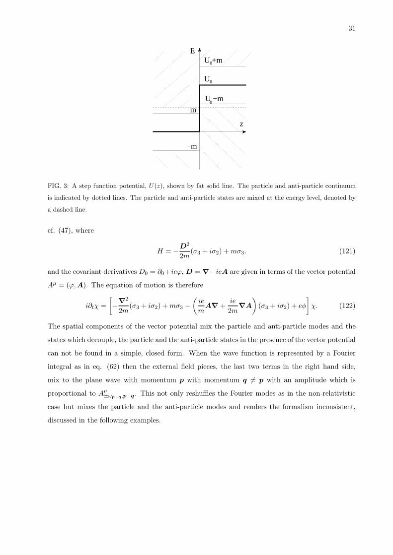
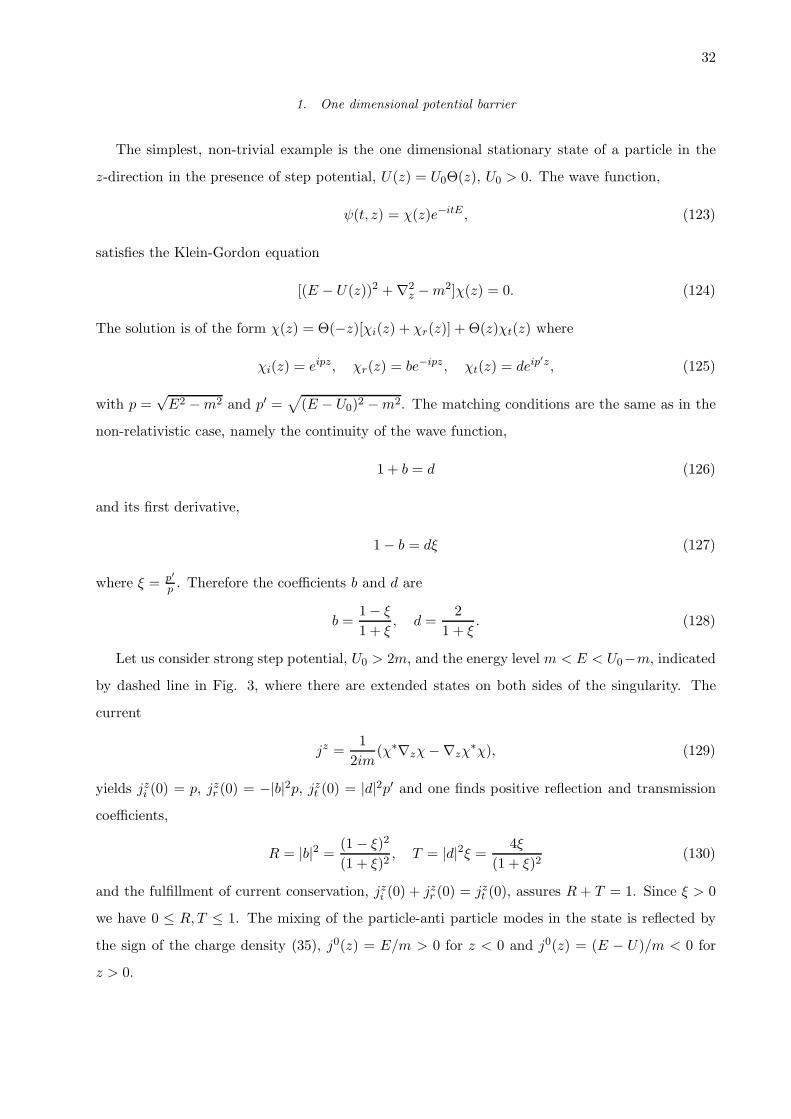
FIG. 3: A step function potential, U(z), shown by fat solid line. The particle and anti-particle continuum
is indicated by dotted lines. The particle and anti-particle states are mixed at the energy level, denoted by
a dashed line.
cf. (47), where
H = −D2
2m(σ3 + iσ2) +mσ3. (121)
and the covariant derivatives D0 = ∂0+ieϕ, D = ∇−ieA are given in terms of the vector potential
Aµ = (ϕ,A). The equation of motion is therefore
i∂tχ =
[
−∇2
2m(σ3 + iσ2) +mσ3 −
(
ie
mA∇+
ie
2m∇A
)
(σ3 + iσ2) + eφ
]
χ. (122)
The spatial components of the vector potential mix the particle and anti-particle modes and the
states which decouple, the particle and the anti-particle states in the presence of the vector potential
can not be found in a simple, closed form. When the wave function is represented by a Fourier
integral as in eq. (62) then the external field pieces, the last two terms in the right hand side,
mix to the plane wave with momentum p with momentum q 6= p with an amplitude which is
proportional to Aµ±ωp−q ,p−q. This not only reshuffles the Fourier modes as in the non-relativistic
case but mixes the particle and the anti-particle modes and renders the formalism inconsistent,
discussed in the following examples.
32
1. One dimensional potential barrier
The simplest, non-trivial example is the one dimensional stationary state of a particle in the
z-direction in the presence of step potential, U(z) = U0Θ(z), U0 > 0. The wave function,
ψ(t, z) = χ(z)e−itE , (123)
satisfies the Klein-Gordon equation
[(E − U(z))2 +∇2z −m2]χ(z) = 0. (124)
The solution is of the form χ(z) = Θ(−z)[χi(z) + χr(z)] + Θ(z)χt(z) where
χi(z) = eipz, χr(z) = be−ipz, χt(z) = deip′z, (125)
with p =√E2 −m2 and p′ =
√
(E − U0)2 −m2. The matching conditions are the same as in the
non-relativistic case, namely the continuity of the wave function,
1 + b = d (126)
and its first derivative,
1− b = dξ (127)
where ξ = p′
p . Therefore the coefficients b and d are
b =1− ξ1 + ξ
, d =2
1 + ξ. (128)
Let us consider strong step potential, U0 > 2m, and the energy level m < E < U0−m, indicated
by dashed line in Fig. 3, where there are extended states on both sides of the singularity. The
current
jz =1
2im(χ∗∇zχ−∇zχ
∗χ), (129)
yields jzi (0) = p, jzr (0) = −|b|2p, jzt (0) = |d|2p′ and one finds positive reflection and transmission
coefficients,
R = |b|2 = (1− ξ)2(1 + ξ)2
, T = |d|2ξ = 4ξ
(1 + ξ)2(130)
and the fulfillment of current conservation, jzi (0) + jzr (0) = jzt (0), assures R+ T = 1. Since ξ > 0
we have 0 ≤ R,T ≤ 1. The mixing of the particle-anti particle modes in the state is reflected by
the sign of the charge density (35), j0(z) = E/m > 0 for z < 0 and j0(z) = (E − U)/m < 0 for
z > 0.

33
z
−m
m
E
−U +m
−U −m
0
0
−U0
FIG. 4: A spherical potential well, U(r), using the convention of Fig. 3.
2. Spherical potential well
As another example we consider the Oppenheimer-Schiff-Snyder effect, displayed by a particle
moving in a spherical potential, U(u). The Klein-Gordon equation assumes the form
[(∂0 + iU(r))2 −∆+m2]φ(x) = 0 (131)
whose stationary states will be sought in the parametrization
φlm(x) = ηℓ(r)Yℓm(θ, φ)e−itE . (132)
The radial wave function of a given ℓ-shell satisfies the equation
[
(E − U(r))2 +1
r2∂rr
2∂r −l(l + 1)
r2−m2
]
ηℓ(r) = 0. (133)
It is advantageous to separate the radial integral measure by writing η(r) = u(r)/r and
[
∂2r −l(l + 1)
r2+ (E − U(r))2 −m2
]
uℓ(r) = 0. (134)
Let us consider an attractive square well potential, U(r) = −U0Θ(r − R), and look for the
stationary states with energy −m < E < m and E > m− U0, allowing the mixing of the particle
and anti-particle modes, cf. Fig. 4. We consider the s-wave sector, ℓ = 0, only for the sake of
simplicity where the radial wave function obeys the equation
u′′0 = [m2 − (E − U(r))2]u0. (135)
34
The solution for r < R is
u0 = sinκr (136)
with κ =√
(E + U0)2 −m2, the component cos κr being suppressed by the regularity of the wave
function at the origin, uℓ(0) = 0. In the exterior region, r > R, we have
u0 = ae−kr (137)
with k =√m2 − E2. The matching conditions,
sinκR = ae−kR, κ cos κR = −kae−kR (138)
yield the transcendental equation
tanRκ = −κk, (139)
whose more detailed form,
tanR√
(E + U0)2 −m2 = −√
(E + U0)2 −m2
m2 − E2, (140)
can be solved graphically. One can easily see an interesting qualitative feature, namely there are
more and more solutions as U0 →∞, shown qualitatively in Fig. 5. As U0 is increases the extended
particle and anti-particle modes, influenced less by the potential, decrease their energy, as expected.
But some bound states are formed withing the forbidden gap, coming both from the particle and
the anti-particle continuum. Note that there are values of U0 which produce two bound states,
corresponding to the same continuous curve in Fig. 5. This is the first surprise, namely the same
potential can bind both particles and anti-particles. The other surprise appear as U0 is increase
until the two bound states coincide where the curve has vertical slope. The system lost a particle
and an anti-particle state at this point. The energy level, given by the matching condition, (140),
becomes complex at this point indicating that this is an unstable, virtual particle-anti particle pair
which can penetrate up a finite distance into the forbidden, r > R region.
III. FERMIONS
A. Heuristic derivation of Dirac equation
By following Dirac’s intuitive derivation we seek an equation of motion which is of first order in
the space-time derivatives by taking formally the square root of the Klein-Gordon equation (31).
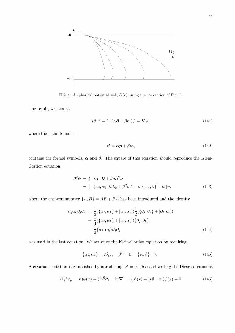
35
U
mE
−m
0
FIG. 5: A spherical potential well, U(r), using the convention of Fig. 3.
The result, written as
i∂0ψ = (−iα∂ + βm)ψ = Hψ, (141)
where the Hamiltonian,
H = αp+ βm, (142)
contains the formal symbols, α and β. The square of this equation should reproduce the Klein-
Gordon equation,
−∂20ψ = (−iα · ∂ + βm)2ψ
= [−{αj , αk}∂j∂k + β2m2 −mi{αj , β}+ ∂j ]ψ, (143)
where the anti-commutator {A,B} = AB +BA has been introduced and the identity
αjαk∂j∂k =1
2({αj , αk}+ [αj, αk])
1
2({∂j , ∂k}+ [∂j , ∂k])
=1
4({αj , αk}+ [αj, αk]){∂j , ∂k}
=1
2{αj , αk}∂j∂k (144)
was used in the last equation. We arrive at the Klein-Gordon equation by requiring
{αj , αk} = 2δj,k, β2 = 11, {α, β} = 0. (145)
A covariant notation is established by introducing γµ = (β, βα) and writing the Dirac equation as
(iγµ∂µ −m)ψ(x) = (iγ0∂0 + iγ∇−m)ψ(x) = (i∂/ −m)ψ(x) = 0 (146)

36
where the constraints (145) are
{γµ, γν} = 2gµν = 2
1 0 0 0
0 −1 0 0
0 0 −1 0
0 0 0 −1
. (147)
Covariance with respect to Lorentz transformation requires that the objects γµ transform as con-
travariant four-vectors.
The “square” of Dirac equation, calculated before can now be written in a simple, covariant
form,
(i∂/−m)(i∂/ +m) = −∂2 −m2. (148)
One can show that the simplest realization of the objects α and β is in terms of 4× 4 matrices,
β = γ0 =
11 0
0 −11
, α =
0 σ
σ 0
, γ =
0 σ
−σ 0
, (149)
and any other set of 4 × 4, verifying the same conditions, (145), can be obtained by a unitary
transformation.
The hermitian conjugate of the wave function satisfies the equation of motion
i∂µψ†(x)㵆 + ψ(x)m = 0. (150)
Since some of the the Dirac matrices, γµ, are not Hermitian, γ0† = γ0, γj† = −γj, this equation is
not covariant. But it is easy to find a linear combination of the components of ψ† which satisfies
covariant equation of motion. The starting point is the relation
γ0γµγ0 = 㵆 (151)
which suggests that the Dirac conjugate,
ψ = ψ†γ0, (152)
will satisfy covariant equation. In fact, inserting 㵆 of eq. (151) into eq. (150) we find
i∂µψγµ + ψm = 0. (153)
But there is an important difference between the use of the Klein-Gordon and the Dirac conjugation.
The former is used in the definition of the scalar product to render the Hamiltonian (48) Hermitian.
37
The Hamiltonian (142) is Hermitian from the very beginning when the matrix α, given by eq. (149)
is used together with the usual Hermitian conjugate in the scalar product,
〈ψ|ψ′〉 =∫
d3xψ†(x)ψ′(x). (154)
The Dirac conjugate, ψ, appears only as an auxiliary variable to make the equation of motion for
ψ† covariant.
The Dirac-equation can be derived as an Euler-Lagrange equation from the Lagrangian
L =i
2[ψγµ(∂µψ)− (∂µψ)γ
µψ]−mψψ. (155)
The Noether current of the U(1) symmetry, ψ(x)→ eiθψ(x), ψ(x)→ e−iθψ(x) is
jµ = ψγµψ. (156)
An important difference compared to the Klein-Gordon equation driven scalar particle is that the
conserved current of an equation of motion which is a first order differential equation contains no
derivative. As a result j0 = ψ†ψ is positive definite and no states with negative norm arise.
The derivation of the Dirac equation, presented above is simple and heuristic but leaves the
physical interpretation of the Dirac space, the four dimensional linear space of the Dirac spinor,
ψa, unclear. To have better understanding of the role played by these components we re-derive
eq. (146) as the simplest equation which governs an elementary particle, equipped with relativistic
symmetries.
B. Spinors
The four dimensional Dirac-space, emerging from the heuristic argument, has physically inter-
pretable structure. To discover it we need a rather lengthy detour into the representation of the
space-time symmetries, realized by spin half particles.
1. Non-relativistic spinors
Elementary systems: Elementary quantum systems are defined with respect to their sym-
metry properties. Suppose that we know that our system under consideration is lacking of any
internal structure and displays a symmetry with respect to transformations, belonging to a group,
G. Therefore there is a linear, unitary or anti-unitary operator, U(g), corresponding to each sym-
metry transformation which acts in the linear space of states and this representation of the group
preserves the algebraic structure of group multiplication, U(gg′) = U(g)U(g′).
38
What can be the consequence in this algebraic structure that our system is elementary? It is
natural to expect that any state can be obtained from a fixed state, |ψ0〉, by the application of
symmetry transformations. In fact, suppose that this is not true and there is a state |ψ′〉 which is
not in the linear space generated by the set of vectors U(g)|ψ0〉, g ∈ G. Then we can safely ignore
the state |ψ′〉 in the discussion of our elementary system because it plays no role in realizing the
symmetry and its inaccessibility by the application of symmetry transformations should come from
some internal structure. The possibility of generating all states of the system from an arbitrary
but fixed state is called irreducibility. The states of an elementary system with a symmetry group
G are therefore vectors of irreducible representation of G.
The construction of irreducible representation is quite different for discrete and continuous
groups. This is the reason that one carefully separates these cases and considers first the con-
nected components of symmetry groups only. For instance, spatial rotations in n-dimensions,
x → Rx, are realized by n × n orthogonal matrices, RtrR = 11 and the determinant of this equa-
tion, (detR)2 = 1, assures detR = ±1 because the determinant of a real matrix is real. The
determinant is a continuous function of the matrix elements, hence the group O(n) has two discon-
nected components, O±(n) = {R|RtrR = 11, detR = ±1}. The subset O+(n) = SO(n) contains
the identity and is a subgroup. It is easy to establish a bijective relation between O+(n) and
O−(n), it is given by the inversion of a coordinate, P1 : (x1, x2, . . . , xn) → (−x1, x2, . . . , xn) or
spatial inversion, P : x→ −x. In fact, we have O−(n) = P1O+(n) and O−(n) = P1O+(n) in even
or odd dimensions, respectively. One works out the irreducible representation for SO(n) first and
extends them over O(n) in the second step.
Irreps of SO(3): It is known that the irreducible representations of the rotation group G =
SO(3) are given by the rotational multiplets,
HJ =
{
J∑
m=−J
cm|J,m〉}
, (157)
of dimension 2J + 1 where J is integer, J = 0, 1, . . . , or half-integer, J = 12 ,
32 , . . .. Thus the
states of elementary systems with a rotational degree of freedom can be represented by the linear
superposition of basis vectors {|J,m〉} for some J . Any representation can be written as the direct
sum of irreducible representations, justifying our definition of elementary system by means of its
symmetry properties.
Tensors and spinors are the wave functions belonging to states with integer and half-integer
angular momentum J , respectively. The difference between them is their response to rotations by
2π. Let us denote the matrix performing a rotation by angle α around the axis n by Rn(α). We
39
have
U(Rn(α)) = e−iαnL (158)
where L is the angular momentum operator and the Wigner matrix elements,
D(J)m,m′(Rn(α)) = 〈J,m|e−iαnL|J,m′〉, (159)
satisfy the equation
D(J)m,m′(Rn(2π)) = δm,m′e−2πim =
+1 J = integer,
−1 J = half integer.
(160)
The simplest non-trivial, tensor and vector representations belong to J = 12 and 1, respectively.
H1 is span by the three-vector x and vectors ψ = (ψ1, ψ2) of the two dimensional H1/2 are called
rotational spinors.
Fundamental representation of SU(2): We first show that the representations of the group
SU(2) can be considered as the representations of the rotation group, SO(3). This circumstance
provides us a simple way to generalize the non-relativistic spinors, defined by the rotation group,
for relativistic spinors, corresponding to the Lorentz group. Let us consider a linear combination
of Pauli matrices and the identity,
A(a,a) = a11 + iaσ =
a+ ia3 ia1 + a2
ia1 − a2 a− ia3
, (161)
where a and a are real numbers, constrained by the condition
detA(a,a) = a2 + a2 = 1. (162)
Such a matrix structure is preserved under multiplication. In fact, identity
σaσb = 11δab + iǫabcσc (163)
can be used to write the product of two such matrices as
A(a,a)A(b, b) = A(ab− ab, ab+ ba− a× b). (164)
Furthermore, this result shows that A−1(a,a) = A(a,−a) = A†(a,a) hence these matrices form
the group SU(2). Another parametrization of the SU(2) matrices, better known in quantum
mechanics, is
An(α) = e−i2αnσ = 11 cos
α
2− inσ sin
α
2, (165)
40
with n2 = 1.
The non-relativistic SU(2) spinor is a two component quantity, ψa, a = 1, 2, transforming
according to the fundamental representation of the group SU(2), ψ → Aψ, and can be interpreted
as a wave function. Having two components, the state, represented by this wave function should
have spin s = 1/2. The complex conjugate of this transformation rule, η → A∗η, yields another two
dimensional representation. But this is unitary equivalent with the fundamental representation.
Two representations, U(g) and U ′(g), are unitary equivalent if there is g-independent unitary
operator, V , which brings it into the other, U ′(g) = V †U(g)V . In fact, the equation
(iσ)∗ = σ2iσσ2 = σ†2iσσ2 (166)
can be used to establish A∗ = σ2Aσ2. This equation together with eq. (163) define the Pauli
matrices.
Adjoint, vector representation of SU(2): The simplest higher dimensional, so called adjoint
representation consists of two index spinors, Xab, a, b = 1, 2, considered as a matrix, transforming
as
X → AXA†, (167)
indicating that the left and the right indices transform according to the fundamental representation
and its complex conjugate, respectively. This representation is 8 dimensional but note that if X
is Hermitian then this property is preserved. Thus it is advantageous to focus our attention to
Hermitian matrices which can be written as
X(xµ) = x011 + xσ =
x0 + x3 x1 − ix2
x1 + ix2 x0 − x3
, (168)
with real coefficients xµ. Note that detX is preserved during this transformation. This matrix can
be considered as the spin wave function of two spin half particles where we use a basis which is
transformed by the unitary matrix σ2 for the particle of the right index. The rule 12 ⊗ 1
2 = 0⊕ 1 of
the addition of angular momentum suggests that we have a spin zero singlet and a spin one triplet
subspaces. It is clear that the former belongs to the component x0, being invariant under SU(2)
transformations.
Relation between SO(3) and SU(2): Now we show that the triplet multiplet is realized by
the components (x1, x2, x3) = x. The length of the vector x, being related to the determinant,
detX = −x2, is preserved by the SU(2) transformation, given by (167). We therefore have found
a linear, length preserving transformation of three-vectors for each SU(2) group elements. The
41
group SU(2) has the same dimension as SO(3) which makes it possible that the different SU(2)
transformations cover the group SO(3). To prove that this possibility is indeed realized it is
sufficient to consider infinitesimal SU(2) transformation using the parametrization (165),
An(α)X(0,x)A†n(α) ≈
(
11− iα2nσ)
xσ(
11 + iα
2nσ)
≈ xσ − iα2[nσ,xσ]
= X(0,x + αn× x), (169)
which is indeed an infinitesimal rotation. The repeated application of this argument establishes
the result for finite α.
Topology: We have just proven is that the transformation (167) realizes a mapping, SU(2)→SO(3), A → R(A). The image is not the full O(3) group because the repetition of infinitesimal
rotations can cover the connected subgroup, SO(3) only.
Our mapping SU(2)→ SO(3) is a two-to-one since R(−A) = R(A). Though the group manifold
SU(2) is simply connected this mapping shows that the group SO(3) has multiply connected
topology: In fact, the diametrically opposite SO(3) rotations, Rn(π) and Rn(−π), are identical
because one is obtained from the other by rotation by 2π, a symmetry transformation of vectors.
Hence a closed loop in the SO(3) group manifold which starts at 11, passes to Rn(π), “jumps“ to
Rn(−π) and returns back to 11 can not be deformed in a continuous manner into a closed loop
passing by 11 and not using the relation Rn(π) = Rn(−π), cf. Fig. 6. On the contrary, any
closed loop can be deformed continuously to a single point in SU(2) which has the topology of a
three-sphere, cf. eq. (162). The spinors transforms as ψ → −ψ under rotation by 2π and they are
preserved by rotation α = 4π.
2. Projective representations
The vectors |ψ〉 and eiα|ψ〉 represent the same physical state hence the representation,U(g), is
to be generalized to a projective representation,
U(gg′) = U(g)U(g′)eiα(g,g′), (170)
where the function α(g, g′) is arbitrary, except that group multiplication should remain associative,
α(g3, g2g1) + α(g2, g1) = α(g3, g2) + α(g3g2, g1). The obvious question which arises at this point is
whether this phase can be eliminated by a ”gauge transformation“, U(g)→ U(g)eiβ(g). There are
two conditions to satisfy if we want to reduce a projective representation of a connected group to
a non-projective representation:
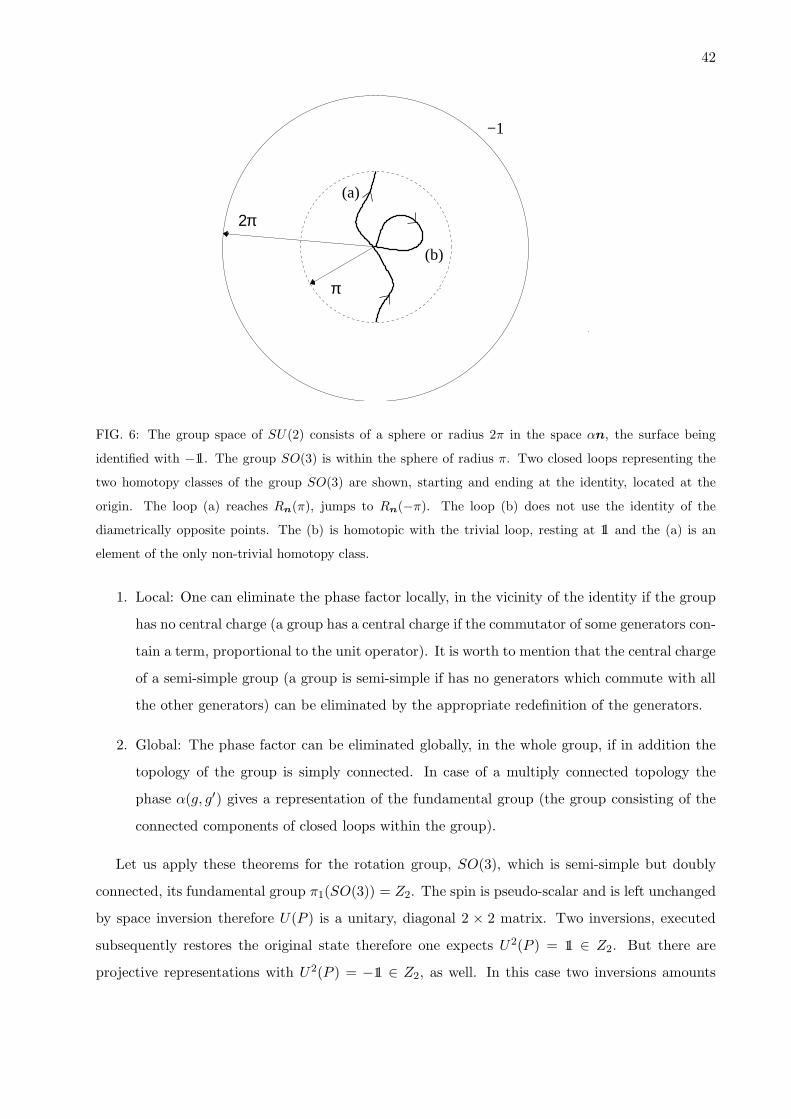
42
(a)
(b)
−1
2π
π
FIG. 6: The group space of SU(2) consists of a sphere or radius 2π in the space αn, the surface being
identified with −11. The group SO(3) is within the sphere of radius π. Two closed loops representing the
two homotopy classes of the group SO(3) are shown, starting and ending at the identity, located at the
origin. The loop (a) reaches Rn(π), jumps to Rn(−π). The loop (b) does not use the identity of the
diametrically opposite points. The (b) is homotopic with the trivial loop, resting at 11 and the (a) is an
element of the only non-trivial homotopy class.
1. Local: One can eliminate the phase factor locally, in the vicinity of the identity if the group
has no central charge (a group has a central charge if the commutator of some generators con-
tain a term, proportional to the unit operator). It is worth to mention that the central charge
of a semi-simple group (a group is semi-simple if has no generators which commute with all
the other generators) can be eliminated by the appropriate redefinition of the generators.
2. Global: The phase factor can be eliminated globally, in the whole group, if in addition the
topology of the group is simply connected. In case of a multiply connected topology the
phase α(g, g′) gives a representation of the fundamental group (the group consisting of the
connected components of closed loops within the group).
Let us apply these theorems for the rotation group, SO(3), which is semi-simple but doubly
connected, its fundamental group π1(SO(3)) = Z2. The spin is pseudo-scalar and is left unchanged
by space inversion therefore U(P ) is a unitary, diagonal 2 × 2 matrix. Two inversions, executed
subsequently restores the original state therefore one expects U2(P ) = 11 ∈ Z2. But there are
projective representations with U2(P ) = −11 ∈ Z2, as well. In this case two inversions amounts

43
to a rotation by 2π, an invisible transformation in classical physics. We have therefore either
U(P ) = ±11 (U2(P ) = 11) or U(P ) = ±i11 (U2(P ) = −11).Every rotation by 2π is represented by the same transformation, Rn(2π) = 11 in SO(3) and
An(2π) = −11 in SU(2). The family of rotations with 0 < α < 2π generate a topological non-
trivial closed loop in the group space. Therefore U(Rn(2π)) = 11eiθ, there the phase factor gives
a representation of the fundamental group, π1(SO(3)) = Z2. This restricts the three-dimensional
particles to being bosons (θ = 0) or fermions (θ = π). The fundamental group is two dimensional
rotations is larger, π1(SO(2)) = Z, the additive group of integers, each homotopy class is charac-
terized by the winding number of the loops. As a result the phase θ is arbitrary in two dimensions,
the two dimensional edge states of the quantum Hall effects are anyons.
3. Relativistic spinors
Fundamental representation of SL(2c): It is not difficult to find spinors for the Lorentz
group along the line of though of the non-relativistic construction. One starts with SL(2, c) groups,
consisting of complex 2 × 2 matrices with unit determinant and its fundamental representation
realized by SL(2, c) spinors, as ψ → Aψ. The parametrization (161), subject of the constraint
(162) remains valid for SL(2, c) matrices except that a and a are complex numbers. Therefore
SL(2, c) is a six dimensional group. The generalization of the parametrization (165) is obtained
by letting α complex.
An important difference with respect to the non-relativistic, SU(2) spinors is that the fun-
damental representation and its complex conjugate are not unitary equivalent anymore because
(166) is insufficient to establish the unitary equivalence for complex α. We follow van der Waerden
conventions for SL(2, c) spinors and use the notation a = 1, 2 and a = 1, 2 for the indices of the
fundamental and the complex conjugate spinor representation where the SL(2, c) transformation
rules are
ξa → A ba ξb, ηa → A∗b
a ψb, (171)
Furthermore, there are covariant and contravariant spinors because
gab =
0 1
−1 0
= iσ2 = −gab (172)
plays the role of the metric tensor since the scalar product remains invariant under SL(2c) trans-
44
formation,
ξaχa = ξag
abχb = ξ1χ2 − ξ2χ1 → (ξaχb − ξbχa)Aa1 A
b2 = (ξ1χ2 − ξ1χ2) detA
ba = ξaχ
a. (173)
The metric tensor is the same for the spinors and complex conjugate spinors.
Lorentz group and SL(2c): Let us now consider the adjoint representation of SL(2, c),
obeying the transformation rule of (167) where the matrix A is now belong to SL(2, c) and the
matrix (168) has the indices Xab(xµ). Another version of this matrix is
Xaa = gabgabXbb = iσ2(x
011 + xσ)iσtr2 = x011− xσtr. (174)
The preservation of detX(x) = x2 makes it plausible that the adjoint representation, (167), is a
Lorentz transformation of xµ. This is certainly the case for the subgroup SU(2) ⊂ SL(2, c) has wehave seen in the previous Chapter. The remaining, other three dimensions of SL(2, c) belong to
imaginary α of the parametrization (165),
An(iβ) = eβ2nσ = 11 cosh
β
2+ nσ sinh
β
2, (175)
and the transformation with infinitesimal β,
An(iβ)X(x0,x)A†n(iβ) ≈
(
11 +β
2nσ
)
(x011 + xσ)
(
11 +β
2nσ
)
≈ x011 + (x+ x0βn)σ +β
2{nσ,xσ}
= X(x0 + βnx,x+ x0βn), (176)
indeed represents a Lorentz boost with infinitesimal velocity v = cβn. It is easy to see that neither
time nor space inversion can be generated in this manner. Thereby we obtained a two-to-one
correspondence between SL(2, c) and the proper Lorentz group, L↑+ and the simplest, spin half
elementary objects are described by spinors ξa or ηa.
Topology: The topology of SU(2) = {An(α)} is S3, the Lorentz boosts manifold, {An(−iβ)},is topologically equivalent with R3 hence the manifold SL(2, c) has the same topology than S3 ⊗R3, i.e simply connected. The SL(2, c) matrices A and −A have identical effect in the adjoint
representation hence the topology of the proper Lorentz group is double connected, π1(L↑+) = Z2.
1. P : As far as P 2 is concerned we have the same possibilities as in the non-relativistic case,
P 2 = ±11. But the representation of P is rendered more involved than for non-relativistic
rotations because the Lorentz boost, Lv, contains the spatial components of a four-vector
which itself is changed by space inversion. The result, PL(v) = L(−v)P 6= L(v)P , implies

45
that space inversion can not be represented by a multiplication of the relativistic spinor com-
ponents with a common phase factor as in the non-relativistic case. Therefore the irreducible
representation of L↑+∪L↑
− is constructed by means of the direct sum of two irreducible repre-
sentations of L↑+. The simplest possibility is to take two spin half representations, consisting
of the bi-spinors
ψ =
ξa
ηa
, (177)
as a four dimensional reducible representation of the proper Lorentz group. One uses the
fundamental representation and its complex conjugate to be able to introduce later the matrix
Xaa(pµ), representing the four-momentum in the equation of motion. Another advantage of
this choice, to be demonstrated in Section IIIB 4, is that the anti-particle of ξ (η) can be
represented by η (ξ).
The space inversion is represented by the transformation
Pξa = zP ηa, Pηa = zP ξa. (178)
on bi-spinors, where zP = ±1 (P 2 = 11) or ±i (P 2 = −11). The sign of zP drops out from
expectation values but the sign of P 2 leads to different transformation rules for complex
conjugate bi-spinors and influences the construction of real bi-spinors. But as long as we do
not want to use our scheme to describe neutral fermions we can ignore this sign.
2. T : The time inversion does not commute with Lorentz boosts in a manner similar to the
space inversion but we can represent it within the same spinor representation of the proper
Lorentz group because T is an anti-unitary operation which changes the sign of the spin. It
should not mix the particle with anti-particle thus we take
Tξa = zT gabξ∗b, T ηa = zT g
abη∗b , (179)
the multiplication with the spinorial metric tensor being the only covariant way of flipping
the spin and zT = ±i to satisfy
T 2 = U(Rn(2π)) = −11. (180)
3. C: The charge conjugation exchanges particles and anti-particles and flips the spin, therefore
we use the representation
Cξa = zCgabη∗a, Cηa = −zCgabξ∗b (181)

46
where zC = ±1 or ±i.
The convention, usually followed in a PTC-symmetric quantum field theory, is zP = −zT = −zC =
i.
4. Dirac equation
The ingredients of an equation of motion for a free particle are the bi-spinor ψ = (ξa, ηa) and
the energy-momentum four-vector paa = p011 + pσ. The only possibility to combine these element
in a linear fashion is
paaηa = mξa,
paaξa = mηa, (182)
where m is a constant of mass dimension. One could use different masses in the two equation but
by an appropriate rescaling of the spinors the two masses become identical. Note that the mass
serves as a coupling constant between the two spinors which decouple in the massless limit where
we can have a covariant equation of motion for one spinor only. the set of equations (182) can be
written in a more explicit manner as
(p0 + pσ)η = mξ,
(p0 − pσ)ξ = mη. (183)
By the elimination of one spinor one arrives at the second order equations
(p2 −m2)ξ = (p2 −m2)η = 0. (184)
The first order equation, eq.(182), can be brought into a simpler form of eq. (146) by pµ = i∂µ
and the introduction of the matrices
γ0ch =
0 1
1 0
, γjch =
0 −σjσj 0
(185)
which are related to the ”standard“ Dirac matrices, given by eq. (149) by the basis transformation
γµch = UγµU †, U =1√2(1− γ5γ0) = 1√
2
11 −1111 11
, (186)
where
γ5 = iγ0γ1γ2γ3, (187)
47
assuming the form
γ5 =
11 0
0 −11
(188)
in chiral representation.
In the presence of an external vector potential, Aµ with minimal coupling, pµ → pµ − eAµ,
∂µ → ∂µ + ieAµ, the Dirac equation is
(i∂/− eA/ −m)ψ = 0 (189)
and the discrete inversions, identified by requiring that the transformed equation of motion remains
covariant, assume the following form:
• Pψ = UPψP , fP (t,x) = f(t,−x), AµP (t,x) = (φ(t,x),A(t,x))P = (φ(t,−x),−A(t,−x)),
UP = iγ0, UP γ0U−1
p = γ0, UPγU−1P = −γ, (i∂/ − eA/P −m)ψP = 0,
• Tψ = UT ψT , fT (t,x) = f(−t,x), AµT (t,x) = (φ(t,x),A(t,x))P = (−φ(−t,x),A(−t,x)),
UT = −iγ1γ3γ0, UTγ0U−1
T = γtr0, UTγU−1T = −γtr, (i∂/ − eA/T −m)ψT = 0,
• Cψ = UCψ, UC = −iγ2γ0, UCγµU−1
C = −γtrµ, (i∂/ + eA/−m)ψC = 0.
We turn our attention to the transformation properties of the bi-spinor under proper Lorentz
transformations. Let us use the parametrization (161) for SL(2, c) matrices with a,a being complex
numbers and write the transformation of the ξ spinor as ξ → A(a,a)ξ. The complex conjugation,
A∗(a,a) = σ2A(a∗,a∗)σ2, (190)
cf. (166), and the displacement of the van der Waerden indices,
A ba = gaa′g
bb′Aa′
b′ , (191)
with g = iσ2 yields
η → iσ2A∗(a,a)iσtr2 η = A(a∗,a∗)η. (192)
Hence the proper Lorentz transformations, An(α+ iβ), can be parametrized by two three-vectors,
u = αn and v = βn which can be rearranged in an anti-symmetric tensor,
ωµν =
0 v1 v2 v3
−v1 0 u3 −u2−v2 −u3 0 u1
−v3 u2 −u1 0
(193)
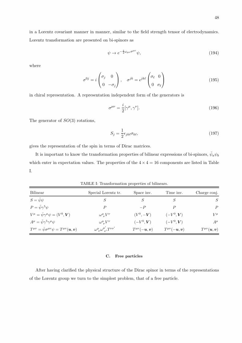
48
in a Lorentz covariant manner in manner, similar to the field strength tensor of electrodynamics.
Lorentz transformation are presented on bi-spinors as
ψ → e−i4ωµνσµν
ψ, (194)
where
σ0j = i
σj 0
0 −σj
, σjk = ǫjkℓ
σℓ 0
0 σℓ
(195)
in chiral representation. A representation independent form of the generators is
σµν =i
2[γµ, γν ]. (196)
The generator of SO(3) rotations,
Sj =1
2ǫjkℓσkℓ, (197)
gives the representation of the spin in terms of Dirac matrices.
It is important to know the transformation properties of bilinear expressions of bi-spinors, ψaψb
which enter in expectation values. The properties of the 4× 4 = 16 components are listed in Table
I.
TABLE I: Transformation properties of bilinears.
Bilinear Special Lorentz tr. Space inv. Time inv. Charge conj.
S = ψψ S S S S
P = ψγ5ψ P −P P P
V µ = ψγµψ = (V 0,V ) ωµ
νV ν (V 0,−V ) (−V 0,V ) V µ
Aµ = ψγ5γµψ ωµ
νV ν (−V 0,V ) (−V 0,V ) Aµ
T µν = ψσµνψ = T µν(u,v) ωµ
νωµ
′
ν′T νν′
T µν(−u,v) T µν(−u,v) T µν(u,v)
C. Free particles
After having clarified the physical structure of the Dirac spinor in terms of the representations
of the Lorentz group we turn to the simplest problem, that of a free particle.

49
1. Plane wave solutions
Let us now consider the plane waves solutions,
ψ(+)(x) = e−ipxup, ψ(−)p (x) = eipxvp (198)
where p0 = ωp ≥ 0 and the bi-spinors up and vp satisfy the equations
(p/−m)up = (p/+m)vp = 0 (199)
with p2 = m2c2 due to Eq. (148). The construction of the spinors up and vp starts in their rest
frame, pµ0 = (mc,0) (m2 > 0),
(γ0 − 1)u0 = (γ0 + 1)v0 = 0, (200)
in particular
u(1)0
=
1
0
0
0
=
φ(1)
0
, u(2)0
=
0
1
0
0
=
φ(2)
0
,
v(1)0
=
0
0
1
0
=
0
χ(1)
, v(1)0
=
0
0
0
1
=
0
χ(2)
. (201)
The bi-spinors corresponding to an arbitrary energy-momentum pµ on the mass shell, p2 = m2c2
are given by
u(α)p =
p/+m√
2m(m+ ωp)u(α)0
=
√
m+ωp
2m φ(α)
σp√2m(m+ωp)
φ(α)
v(α)p =
−p/+m√
2m(m+ ωp)v(α)0
=
σp√2m(m+ωp)
χ(α)
√
m+ωp
2m χ(α)
(202)
according to Eq. (148) where φ(α) and χ(α) are p-independent, two-component spinors. The
normalization is chosen in such a manner that the relations
u(α)p u
(β)p = −v(α)p v
(β)p = δα,β, u
(α)p v
(β)p = v
(α)p u
(β)p = 0 (203)
50
hold. It is easy to see that the current (156) assumes the form (40) for plane waves. Since
j0 = ψγ0ψ = ψ†ψ ≥ 0 the density is non-negative in contrast to the scalar particle.
We present for later use the projection operator corresponding to the positive and negative
energy bi-spinors,
P+(p) =
2∑
α=1
u(α)p ⊗ u(α)p =
p/+m√
2m(m+ ωp)
1 + γ0
2
p/+m√
2m(m+ ωp)=p/+m
2m(204)
and
P−(p) = −2∑
α=1
v(α)p ⊗ v(α)p =
p/−m√
2m(m+ ωp)
1− γ02
p/−m√
2m(m+ ωp)=m− p/2m
, (205)
respectively either by the help of the definition (147) or simply by using eqs. (199).
The four linearly independent plane wave solutions of the free Dirac equation corresponding to
a given (canonical) energy-momentum pµ represent the two spin polarization states of a fermion of
spin half and its anti-particle. The separation of the particle and the anti-particle modes is achieved
in the spinor space as in the case of the first order formalism of the Klein-Gordon equation. The
momentum-dependence of the projectors (204)-(205) indicates that the particle and anti-particles
axes in the spinor space are momentum-dependent, too.
The spinors of the standard and the chiral representation are related by ψ = U †ψch. It is
advantageous to use the parametrization ψ = (φ+, φ−) in standard representation because the
combinations φ± = η ± ξ are such that φ+ (φ−) is made up dominantly by particle (anti-particle)
modes for non-relativistic particles, |p| ≪ m, according to (200). The space inversion which
preserves the piece iγ∇ of the Dirac equation should not change the eigenvalue of γ0 neither in
order to keep the covariance of the equation. Furthermore, time inversion and charge conjugation
change the sign of ∂0 and should therefore flip the eigenvalue of γ0.
2. Spin density matrix
The state of the spin is represented by the spin density matrix, usually written in the non-
relativistic case as
ρ =1
2(11 + aσ), (206)
giving the expectation value
〈S〉 = tr[ρS] =a
2, (207)
51
and the state is mixed if
trρ2 =1
4tr(11 + a2 + 2aσ) =
1 + a2
2< trρ = 1, (208)
i.e., a2 < 1. The relativistically covariant generalization for the particle state (202), is the density
matrix
ρ = u(α)p ⊗ u(α)p . (209)
The expectation value of the spin operator, given by eq. (197),
〈S〉 =∫
d3xψ∗(x)Sψ(x) =
∫
d3xψ(x)γ0Sψ(x), (210)
leads to the relativistically covariant expression
〈S〉 = tr[ργ0S]. (211)
It is sometime useful to express this expectation value in a different form whose derivation starts
with an expression of γ5 involving the Levi-Civita tensor,
γ5 = iγ0γ1γ2γ3 = − i
4!ǫµνρσγ
µγνγργσ, (212)
where the minus sign arises from ǫ0123 = 1, ǫµνρσ = −ǫµνρσ. This equation, multiplied by two Dirac
matrices,
γ5γκγλ = − i
4!ǫµνρσγ
µγνγργσγκγλ, (213)
and evaluated by permuting the indices µ′ and ν ′ to the rightmost poisition in the Levi-Civita
symbol results in
γ5γκγλ = − i2ǫµνλκγ
µγν , (214)
according to eq. (147). This result is now used in the third step of the chain of equations
i
2ǫµνρσσρσ =
i
2ǫµνρσ
i
2[γρ, γσ] = −
1
2ǫµνρσγργσ = γ0γ1γ2γ3γµγν = γ5σµν , (215)
allowing us to bring the spin operator into the form
Sj =1
2ǫjkℓσkℓ =
1
2ǫ0jρσσρσ = −i1
2γ5σ0j = γ5γ0γj. (216)
Finally the anti-commutator, {γ5, γµ} = 0, yields an alternative form
〈S〉 = −tr[ργ5γ] (217)
52
for the spin expectation value.
To find the relativistic generalization of the density matrix (206) we introduce a pseudo-vector,
aµ = (a0,a) which remains invariant under space inversion and becomes aµ0 = (0, 2〈S〉) in the
rest frame, pµ0 = (m,0). Such a structure yields the orthogonality, ap = 0, and invariant length
square a2 = −2〈S〉2. Though the explicit form of aµ is not needed below one can easily find it by
performing the Lorentz boost,
a0 =a00 − va0‖√
1− v2, a‖ =
a0‖ − va00√1− v2
, (218)
with velocity v = −p/p0 where a0‖ = a0p/|p|. The result of the boost is
a0 = 2|p|m〈S‖〉, a⊥ = 2〈S⊥〉, a‖ = 2
p0
m〈S‖〉 (219)
where
S‖ =Sp
|p| , S⊥ =
(
11− p⊗ p
p2
)
S. (220)
The simplest example is the density matrix of an non-polarized state, 〈a〉 = 0 of a particle. It
should be a linear expression of the four momentum, pµ. The form of the projector operator (204)
suggests the form
ρ =p/+m
4m. (221)
The equations
tr[γµ1 · · · γµ2n+1 ] = 0, tr[γµγν ] =1
2tr[{γµγν}] = 4gµν (222)
can be used to check 〈S〉 = 0. The density matrix of a partially polarized state is more involved,
it will be sought in the form,
ρ =1
8m2(p/+m)ρ0(a)(p/ +m) (223)
where ρ0(0) = 11. By assuming that ρ0(a) is a linear function of aµ we write
ρ0(a) = 11 + zγ5a/ (224)
cf. (217) and determine the scalar coefficient z by evaluating the spin average in the rest frame
where aµ0 = (0,a0) and
ρ =1
8(11 + γ0)(11− zγ5aγ0)(11 + γ0) =
1
4(11 + γ0)(11− zγ5a/0). (225)
53
The corresponding spin expectation value,
〈S〉 = −tr[ργ5γ] = −1
4tr[(11 + γ0)(11− zγ5a/)γ5γ], (226)
can be brought into the form
〈S〉 = z
4tr[(11 + γ0)γ5a/γ5γ] = −z
4tr[(11 + γ0)a/γ] = −z
4tr[a/γ] = za (227)
by the help of eqs. (222). The comparison if this result with eq. (207) yields z = 12 ,
ρ =1
8m2(p/+m)
(
11 +1
2γ5a/
)
(p/+m), (228)
and the identity a/p/ = ab− p/a/ = −p/a/ leads to the form
ρ =1
4m(p/+m)
(
11 +1
2γ5a/
)
(229)
of the density matrix. By starting with a given density matrix of this form the parameter aµ can
be extracted by the equation
aµ = −2tr[ργ5γµ]. (230)
To prove this result we start with the identity,
tr
[
(p/+m)
(
11 +1
2γ5a/
)
γ5γµ]
= tr[(
p/+m
2γ5a/)
γ5γµ]
. (231)
To simplify it we use the equation tr[γ5γµγν ] = 0 which can easily be checked separately for the
cases µ = ν and µ 6= ν and leads to
tr
[
(p/+m)
(
11 +1
2γ5a/
)
γ5γµ]
= −m2tr[a/γµ] = −2maµ (232)
Q.E.D. As a cross check we calculate the density matrix in the rest-frame and int the standard
representation,
ρ =1
4(11 + γ0)
(
11 +1
2γ5a/
)
=1
4
2 0
0 0
11− 1
2
0 1
1 0
0 aσ
−aσ 0
=1
4
2 0
0 0
11− 1
2
−aσ 0
0 aσ
=1
2
11 + aσ 0
0 0
(233)
Finally we add that the density matrix for an anti-particle is given by
ρ(−) = UCρ(+)U∗
C . (234)
54
3. Helicity, chirality, Weyl and Majorana fermions
A Dirac fermion is described by a four component, complex bi-spinor and there are different
ways of splitting this eight dimensional vector into two four dimensional ones. We discuss three of
them below.
The helicity is defined as the projection of the total angular momentum of a particle on its
momentum,
hp =Jp
|p| . (235)
The orbital angular momentum drops from this expression,
hp =Sp
|p| , (236)
owing to J = L + s and Lp = 0, hence the helicity of a Dirac fermion is ±~/2. The helicity
commutes with the Hamiltonian (142), [αp + βm,Sp] = 0, and is thereby conserved, c.f. Table
II. It is furthermore invariant under spatial rotations and offers a natural basis to handle the spin
orientations of a free particle. However it changes under Lorentz boosts which mixes the helicity
component. This can be anticipated by noting that it changes sign when we perform a Lorentz
boost with a velocity which is parallel to and larger than the particle velocity. The spin projection
on the direction of the velocity arises from the components of the tensor σkℓ which are orthogonal
to the velocity and thus remain unchanged. But the velocity of the particle changes sign during
the boost, together with the helicity. Thus a massive fermion can not be composed exclusively
from a given helicity components.
TABLE II: Invariance properties of the splitting of the bi-spinor space.
Invariance Helicity Chirality Majorana fermion
L↑+ × X X
Time evolution of a free particle X m 6= 0 : ×; m = 0: X X
The spinor representation of the special Lorentz group in which a massless particle is found can
be equipped with a quantum number, called chirality. It is defined as the eigenvalue of the Dirac
matrix γ5 according to the form (188) in chiral representation. Thus
R =1
2(11 + γ5), L =
1
2(11− γ5), (237)
project onto chirality +1 and −1, called right-handed and left-handed states, respectively. Chi-
rality is a Lorentz invariant quantity but is conserved by massless particles only.
55
Both the helicity and the chirality are conserved by masless particles hence one wonders whether
there is a relation between these quantities. The equation of motion for massless particles,
(∂0 −∇σ)η = 0, (∂0 +∇σ)ξ = 0, (238)
cf. eqs. (183), written in the form
i∂0η = −pση, i∂0ξ = pσξ, (239)
shows that the helicity and the chirality are identical for positive energy massless excitations. The
name helicity refers to the opposite direction of the rotation of the helicity (S = σ/2) for the left
and the right handed spinors.
Weyl fermions, the left or right handed spinors of the special Lorentz group, ξ = Rψ and
η = Lψ, are massless fermions which respect no space inversion. They can be described either by
a spinor ξ or η exclusively and the corresponding equation of motions, (238), can be derived from
the Lagrangian
Lη = η†(i∂0 − i∇σ)η, Lξ = ξ†(i∂0 + i∇σ)ξ. (240)
The Weyl fermions are massless and the first equation in (238) was sometime called neutrino
equation, by now a historic name from the time when neutrinos were thought to be massless.
One can find a basis transformation
UM =1
2
1 + σ2 i(σ2 − 1)
i(1 − σ2) 1 + σ2
(241)
which brings the gamma matrices into the imaginary form, γµM = UγµchU†, in particular
γ0M =
0 σ2
σ2 0
, γ1M =
iσ1 0
0 iσ1
, γ2M =
0 σ2
−σ1 0
, γ3M =
iσ3 0
0 iσ3
, (242)
and thereby renders the Dirac equation real. Its solution preserves the phase and represents a
Majorana fermion.
One may wonder if the four real functions of a Majorana fermion could be compressed in a Weyl
fermion. The difficulty is that the realness of the Dirac fermion wave function, ψ∗ = ψ, is not a
Lorentz invariant condition. But the bi-spinor
ψM =
ξ
−iσ2ξ∗
, (243)

56
given in the chiral representation is brought into a real bi-spinor by the basis transformation (241).
While a Weyl fermion can not have mass the Majorana fermion which has the same number of real
components can. In fact, the Lagrangian
LM =1
2ψM (i∂/ −m)ψM , (244)
is manifest Lorentz invariant and becomes
LM =1
2[ξ†i(∂0 −∇σ)ξ −mξtriσ2ξ] + c.c. (245)
in the chiral representation becomes where c.c. stands for complex conjugation. The corresponding
equation of motion is massive,
(∂0 −∇σ)ξ −mσ2ξ∗ = 0. (246)
The precision tests of the Standard Model should soon reveal if the neutrino masses are generated
for Weyl or Majorana neutrinos.
The construction of the Majorana fermions shows the highly non-trivial structure of the Dirac
matrices, arising from the identity (166). One may go even further and use eq. (168) to represent
the space-time coordinate vectors by spinors, xµ ↔ Xaa(x) ↔ νaν a. To have four dimensional
objects one sets ν = ν∗ and parametrizes the coordinate in terms of the twistor ν,
Xaa(x) = νaν∗a. (247)
However this reduces the dimensionality of X to three because X remains invariant under the
global phase change, ν → eiαν. This is in agreement with the observation that the rank of νaν∗a
is one, giving detX = xµxµ = 0, the twistor parametrization is available for light-like vectors only.
D. Non-relativistic limit
Let us find the non-relativistic limit of the Dirac equation with a vector potential, written as
i
c∂tψ =
[
α(−i∇− e
cA) + βmc+
e
cA0
]
ψ, (248)
where the units c 6= 1 are reintroduced. We shall work in the standard representation, (149), and
write the equation for the bi-spinor ψ = (φ, χ),
i∂tφ = cσπχ+ (eA0 +mc2)φ,
i∂tχ = cσπφ + (eA0 −mc2)χ, (249)
57
where the momentum π = p− ecA is used. To find regular time dependence in the non-relativistic
limit for an electron we separate the rest mass energy in the solution and use Φ = eimc2tφ and
X = eimc2tχ in the equation of motion
i∂tΦ = cσπX + eA0Φ,
i∂tX = cσπΦ + (eA0 − 2mc2)X. (250)
As long as we can neglect the time derivative and eA0 in the second equation compared to mc2 we
can use the approximation
X =σπ
2mcΦ (251)
for the small component of the bi-spinor. Inserting this relation into the first equation we arrive
at Pauli equation for the large component,
i∂tΦ =
[
(σπ)2
2m+ eA0
]
Φ, (252)
suggesting that the influence of the small component is the replacement p→ σπ in the Schrodinger
equation. The identity (163) gives
(σπ)2 = σjσkπjπk = π2 − e
cB (253)
with B = ∇×A and the Pauli equation,
i∂tΦ =
[
(p− ecA)2
2m− e
2mcσB + eA0
]
Φ. (254)
The first term appears in the Schrodinger equation and it reads for a homogeneous magnetic field,
A(x) = 12x×B, as
HSch =p2
2m+eAp
mc=
p2
2m− eLB
2mc. (255)
This form reveals an angular momentum-magnetic field interaction with energy
HL = −µBLB
~, (256)
where µb = e~/2mc is the Bohr magneton. The second term in the equation of motion, (254), can
be written as
HS = −gSµBSB
~(257)
58
where gS = 2 is the gyromagnetic factor. The lesson of the Pauli equation is that the magnetic field
can distinguish the orbital and the spin contribution to the total angular momentum, J = L+S,
because the angular momentum-magnetic field coupling is
HJ = −µB(L+ 2S)B
~(258)
in the non-relativistic limit. An electron continuously emits and absorbs photons during its prop-
agation and these processes change its angular momentum and generate a small non-trivial value
for gS − 2. This value in known experimentally up to twelve decimals and has been checked by
O(
α4)
perturbation calculation. The agreement represents one of the precision tests of quantum
electrodynamics.
Such a treatment of the non-relativistic limit is flowed. One problem is the issue of the velocity:
The Heisenberg equation for the coordinate operator,
i
c∂tx = [x,αp + βmc2] = iα, (259)
shows that the particle moves with the speed of light because the spectrum of αj is ±1. The
average speed becomes small in the non-relativistic limit due to the frequent flip of sign of the
eigenvalues of αj as the state oscillates between the different eigenstates of β. This is actually the
context how Zitterbewegung has been identified as the result of the interference between positive
and negative energy solutions of the Dirac equation.
This result is reasonable, argued Dirac, since the velocity is obtained by two successive mea-
surement in time of the coordinate. The Heisenberg uncertainty principle introduces a large spread
for the momentum when the two coordinate measurements are carried out in short time difference.
The practically uniformly distributed momentum is dominated by large values of momentum, cor-
responding to the velocity of light. There must obviously a way to get through this complication
and arrive at the usual description of a non-relativistic electron in Schrodinger’s wave mechanics.
Another problem of the derivation of the Pauli equation is that the time derivative of the
small component, neglected in the derivation, would introduce higher order time derivatives in the
equation of motion. Such higher order derivative terms, whatever weak they are in the equation
of motion, produce important effects in sufficiently long time. This can be seen by recalling
Ostrogadsky’s theorem, stating that the energy of a classical system whose equation of motion is
canonical, i.e. can be derived from a Lagrangian or Hamiltonian, is unbounded from below. Thus
we loose the stability of the classical equations of motion higher than second order. Since we do
not know the fundamental equations in physics, all we have are effective equations, valid in certain
59
resolution window. These equations are always non-local in time. The non-local equations represent
a far too hard problem to solve hence one usually applies the gradient expansion, truncated at a
certain order. The lesson of Ostrogadky’s theorem is that this procedure is acceptable in dealing
with non-localities in space but can not be applied in time.
A more physical approach of the non-relativistic limit is offered by the Foldy-Wouthuysen
transformation which is a basis transformation, |ψ〉 → S|ψ〉 to decouple the small and the large
components. We look for the the similarity transformation of the form
S = e−γp
|p|θ= 11 cos θ +
γp
|p| sin θ, (260)
where the sign of the sinus is positive owing to (γp)2 = −p2. It transforms the Hamiltonian into
S(αp + βm)S−1 =
(
11 cos θ +γp
|p| sin θ)
(αp+ βm)
(
11 cos θ − γp
|p| sin θ)
= (αp+ βm)
(
11 cos θ − γp
|p| sin θ)2
= (αp+ βm)
(
11 cos 2θ − γp
|p| sin 2θ)
= αp
(
11 cos 2θ − m
|p| sin 2θ)
+ β(m cos 2θ + |p| sin 2θ), (261)
where the equation pjpk{γj , αk} = pjpkγ0[γj , γk] = 0 was used in changing the order of the frist
two factors and in arriving at the second line. The choice
sin 2θ =|p|ωp, cos 2θ =
m
ωp, tan 2θ =
|p|m, (262)
decouples the positive and negative energy modes since
HFW = βωp. (263)
The form of the projectors eqs. (204)-(205) in this base,
SP±(p)S−1 =
(
11 cos θ +γp
|p| sin θ)
m± (βωp − γp)
2m
(
11 cos θ − γp
|p| sin θ)
=m∓ γp
2m± βωp
2m
(
11 cos θ − γp
|p| sin θ)2
=m∓ γp
2m± βωp
2m
(
11m
ωp− γp
|p||p|ωp
)
=11± β2
, (264)
shows explicitly that the positive and negative energy plane wave belong to exactly the upper or
lower components of the bi-spinor in this representation.
60
The velocity operator in this basis, given by the Heisenberg equation of for the coordinate,
1
c∂tx = −i[x, βωp]
= β∇pωp (265)
is the group velocity up to the sign of the energy, the eigenvalue of β.
The momentum dependence of the basis transformation indicates that the coordinate operator
of the Foldy-Wouthuysen representation belongs to
xFW = SxS−1
=
(
11 cos θ +γp
|p| sin θ)
x
(
11 cos θ − γp
|p| sin θ)
= x+ ia (266)
in the original Dirac basis with
a = −∇p
(
γp
|p| sin θ)
. (267)
E. External field
The mixing of the particle-anti particle modes are considered below in the presence of an external
potential.
1. Klein paradox
The first example to consider is the one-dimensional motion in the presence of a potential
barrier, U(z) = U0Θ(z), shown in Fig. 3. The wave function,
ψ(t, z) = χ(z)e−itE , (268)
satisfies the Dirac equation,
[γ0(E − U(z)) + iγz∇z −m]χ(z) = 0. (269)
We assume that U0 > 2m and m < E < −m + U0 to assure the extended incoming particle and
transmitted anti-particle modes in the stationary state. The wave function for z < 0 is the sum of
the incident and the reflected waves, χ = χi + χr, with
χi(z) = eipz
1
0
pm+E
0
61
χr(z) = be−ipz
1
0
− pm+E
0
+ b′e−ipz
0
1
0
pm+E
, (270)
according to eq. (202). The solution for z > 0 describes the transmitted wave,
χt(z) = deip′z
1
0
p′
m+E−U0
0
+ d′eip′z
0
1
0
− p′
m+E−U0
. (271)
The momenta are defined by the equations E2 = m2+ p2 and (E−U0)2 = m2+ p′2. The potential
is spin independent and the spin flip is excluded, b′ = d′ = 0.
To find the matching condition at the singularity of the potential we write the Dirac equation
as
∇zχ(z) = iγz [m− γ0(E − U(z))]χ(z) (272)
and integrate within the interval −ǫ < z < ǫ. The result is that the discontinuity of the wave
function is given by
Discχ(0) = iγz limǫ→0
∫ ǫ
−ǫ[m− γ0(E − U(z))]χ(z). (273)
The right hand side of vanishing for bounded potential therefore we have the matching condition
is
1 + b = d (274)
for the first component of the spinor and
(1− b) p
m+ E= d
p′
m+ E − U0(275)
for the third component. We write the latter as
1− b = dξ (276)
with
ξ =p′
p
m+E
m+ E − U0, (277)

62
yielding
b =1− ξ1 + ξ
, d =2
1 + ξ. (278)
The reflection and transmission coefficients are defined by means of the current,
jz = ψγzψ = ψ†γ0γzψ = χ†
0 σz
σz 0
χ, (279)
as
R = −jrji, T =
jtji. (280)
Since
ji = 2p
m+ E, jr = −2|b|2
p
m+ E, jt = 2|d|2 p′
m+ E − U0, (281)
we have
R = |b|2, T = |d|2 p′
p
m+ E − U0
m+ E. (282)
Note that the current is conserved,
ji(0) + jr(0) =2(1 − |b|2)pm+ E
=2(1− |b|2)p′
ξ(m+ E − U0)= jt(0)
1− |b|2ξ|d|2 = jt(0), (283)
and R+ T = 1. Since ξ < 0 in the considered energy interval we have R > 1 and T < 0, known as
the Klein paradox. Such a process is absent in the second quantized formalism of quantum field
theories.
2. Spherical potential
The solution Dirac equation with a time-independent potential,
i∂0ψ(x) = [αp+ βm+ U(x)]ψ(x), (284)
is sought by factorizing an oscillatory time dependence by the help of the ansatz
ψ(t,x) = ψ(x)e−iEt. (285)
The space-dependent wave function satisfies the stationary Dirac equation,
[αp+ βm+ U(x)]ψ(x) = Eψ(x). (286)
63
In case of a spherically symmetric potential, U = U(r), one obviously uses polar coordinate
system and the directional dependence of the wave function is provided by using the spinor spherical
harmonics
YℓJ,M =
∑
m+σ=M
(ℓ,m,1
2, σ|J,M)Y ℓ
m(θ, φ)φ(σ), (287)
where the usual spherical harmonics satisfy the equgenvalue conditions
L2Y ℓm = ℓ(ℓ+ 1)Y ℓ
m, L3Yℓm = mY ℓ
m, (288)
and the spin states are defined by the conditions
S2φ(σ) =3
4φ(σ), S3φ(σ) = σφ(σ). (289)
The rule of addition of angular momentum, ℓ ⊗ 12 = ℓ − 1
2 ⊕ ℓ + 12 , shows that a given total
angular momentum state, characterized by a given J,M quantum number pair corresponds to a
two-dimensional subspace with orbital angular momentum ℓ = J± 12 . Owing to the transformation
rules under space inversion,
PY ℓm(θ, φ) = (−1)ℓY ℓ
m(θ, φ), PSP−1 = S (290)
these two states with different orbital angular momentum have different parity,
PYℓJ,M (θ, φ) = (−1)ℓYℓ
J,M(θ, φ). (291)
This is an indirect justification of regrouping two irreducible representations of the proper Lorentz
group together to find a representation of the space inversion. In particular,
P
φ(t,x)
χ(t,x)
= iγ0
φ(t,−x)χ(t,−x)
= i
φ(t,−x)−χ(t,−x)
(292)
in the standard representation. Hence the space-dependent component of the bi-spinor with definite
parity, π = (−1)J± 1
2 , can be written into the form
ψ(±)J,M(r, θ, φ) =
1
r
uJ± 1
2
(r)YJ± 1
2
J,M (θ, φ)
ivJ∓ 1
2
(r)YJ∓ 1
2
J,M (θ, φ)
. (293)
To write the stationary Dirac equation in terms of this bi-spinor we need a more appropriate
expression for pα. By the help of the radial unit vector, n = x/r, one can write
(nα)(pα) =
0 nσ
nσ 0
0 pσ
pσ 0
64
= [np+ i(n× p)σ] =
(
np+i
rLσ
)
=
(
−i∂r +i
rLσ
)
, (294)
yielding
pα = (nα)2(pα) = nα
(
−i∂r +i
rLσ
)
. (295)
The next step is to work out the action of nα and Lσ on the spherical harmonics. We start with
the eigenvalue equation for the bi-spinor,
L2ψ(±)J,M =
(J ± 12 )(J ± 1
2 + 1)
(J ∓ 12 )(J ∓ 1
2 + 1)
ψ(±)J,M =
J2 + 14 ± J + J ± 1
2
J2 + 14 ∓ J + J ∓ 1
2
ψ(±)J,M
=
[
J(J + 1) +1
4± β
(
J +1
2
)]
ψ(±)J,M , (296)
giving
Lσψ(±)J,M = (J2 −L2 − S2)ψ
(±)J,M =
[
−1∓ β(
J +1
2
)]
ψ(±)J,M . (297)
The action of the matrix nσ on YJ± 1
2
J,M is found in three steps.
1. First we relate in actions of nσ and Lσ. The equations
(nσ)(Lσ) = i(n ×L)σ =i
rσaǫabcxbǫcdexdpe =
i
r[x(xp)− px2]σ,
(Lσ)(nσ) =i
rǫabcxbpcǫadexdσe =
i
r(ǫabcxbǫadexdpc − iǫabcxbǫace)σe
=i
r[x2pσ − (xσ)(xp) + 2ixσ], (298)
serve to establish
(Lσ)(nσ) = −(nσ)(Lσ) − 2nσ. (299)
2. We apply this equation on YJ∓ 1
2
J,M and use the lower block of eq. (297) to find
(Lσ)(nσ)YJ∓ 1
2
J,M =
[
−1∓(
J +1
2
)]
nσYJ∓ 1
2
J,M . (300)
The comparison of this result with the upper block of eq. (297),
LσYJ± 1
2
J,M =
[
−1∓(
J +1
2
)]
YJ± 1
2
J,M , (301)
shows that nσYJ∓ 1
2
J,M and YJ± 1
2
J,M satisfy the same non-degenerate eigenvalue equations hence
nσYJ∓ 1
2
J,M = aℓYJ± 1
2
J,M . (302)
65
3. The eigenvalues of nσ are ±1 which requires |a| = 1. In the special caseM = J this equation
reads
nσ
1
0
YJ− 1
2
J,J = aℓ
0
1
YJ+ 1
2
J,J , nσ
0
1
YJ+ 1
2
J,J = aℓ
1
0
YJ− 1
2
J,J (303)
since the spin is parallel and anti-parallel with the orbital momentum on the two sides of
the equation. The form Y ℓℓ ∼ [−(x+ iy)]ℓ of the spherical harmonics gives aℓ = a = −1 and
nσYJ∓ 1
2
J,M = −YJ± 1
2
J,M . (304)
We have now all the necessary elements to work out the Dirac equation in terms of our ansatz.
The equations (295) and (297) brings the stationary Dirac equation into the form
[
inα
[
−∂r −1
r∓ 1
rβ
(
J +1
2
)]
+ βm+ U
]
1
r
uJ± 1
2
YJ± 1
2
J,M
ivJ∓ 1
2
YJ∓ 1
2
J,M
= E1
r
uJ± 1
2
YJ± 1
2
J,M
ivJ∓ 1
2
YJ∓ 1
2
J,M
. (305)
The identity (∂r +1r )
fr = f ′
r and eq. (304) allow us to further simplify this result,
−i
0 1
1 0
[
−∂r ∓1
rβ
(
J +1
2
)]
+ βm+ U(r)
uJ± 1
2
ivJ∓ 1
2
= E
uJ± 1
2
ivJ∓ 1
2
(306)
and finally arrive at the equation
[
−∂r ±1
r
(
J +1
2
)]
vJ∓ 1
2
= (E −m− U)uJ± 1
2
,[
∂r ±1
r
(
J +1
2
)]
uJ± 1
2
= (E +m− U)vJ∓ 1
2
. (307)
We can extract an equation for uJ± 1
2
by expressing vJ∓ 1
2
from the second equation and inserting
it into the first equation,
0 =
{
m+ U − E +
[
−∂r ±1
r
(
J +1
2
)]
1
E +m− U
[
∂r ±1
r
(
J +1
2
)]}
uJ± 1
2
. (308)
It is instructive to check the free case, U = 0,
0 =
[
m2 − E2 − ∂2r +1
r2
(
J +1
2
)(
J +1
2± 1
)]
uJ± 1
2
(309)
which is identical with that Klein-Gordon case.
66
3. Spin precession
The non-relativistic dynamics of the spin in the presence of a homogeneous magnetic field, B,
is generated by the modification
H = H0 − µBσB (310)
of the spin-less Hamiltonian where µB = e~2mc . The Heisenberg equation for the spin operator,
S = σ/2,
i∂tS = [S,H], (311)
and [Sj , σk] = iǫjkℓσℓ = 2iǫjkℓSℓ leads to the equation of motion
∂tS = 2µBS ×B. (312)
The expectation value a = 2〈S〉 satisfies the equation of motion
∂ta = 2µBa×B (313)
and performs a precession around the magnetic field. The equation of motion for the spatial motion
in the semi-classical limit,
∂t〈v〉 =e
mc〈v〉 ×B, (314)
shows that the velocity perform a precession with the same frequency and the angle of 〈S〉 and 〈v〉is time-independent.
To find the generalization for the relativistic case we assume that the right hand side of the
equation of motion is linear in Fµν , aµ and at most quadratic in the four velocity, uµ = pµ/m. The
invariance of the equation of motion under spatial inversion prevents the appearance of Fµνuν in
the equation of motion, the anti-symmetry, Fµν = −F νµ, eliminates the term aµF νρuνuρ and the
orthogonality au = 0 excludes the combination Fµνuνau. Therefore one arrives at the equation
∂saµ = αFµνaν + βuµF νρuνaρ, (315)
containing the constants α and β. These parameters can be found by inspecting the equation in
the rest frame, in the limit aµ → (0,a), uµ → (1,0) and s→ t,
∂ta = αa×B. (316)
67
This result imposes α = 2µB . The other parameter is determined by the help of the semi-classical
equation of motion,
uµ =e
mFµνuν , (317)
yielding
ua = −ua = − e
maµF
µνuν (318)
where the time derivative of the orthogonality relation, au = 0, au+ au = 0 was used in the first
equation. Finally eq. (315) is multiplied by u and we arrive at the equation
ua = (2µB + β)uµFµνaν = − e
maµF
µνuν (319)
by the help of u2 = 1 which gives
β =e
m− 2µB (320)
and the relativistic equation of motion
∂saµ = 2µFµνaν +
( e
m− 2µB
)
uµF νρuνaρ. (321)
Appendix A: Multi-valued wave functions
Schrodinger’s wave function, a complex valued function of the space-time coordinates, may be
multi-valued. It is always an exciting question whether a mathematical possibility is realized by
Nature of remains a dead end street of the formalism. In this case the multi-valued nature of the
wave function is related to observable, physical phenomena, of which the Aharonov-Bohm effect
is the simplest. This is a surprising mechanism of quantum mechanics which generates a new
quantum number, without any classical analogy, and an unexpected dependence of expectation
values on this quantum number which may lead to the violation of eqs. (27).
1. Particle on the circle
Let us consider a particle which is restricted into a circle of radius r. The requirement that the
momentum operator, p = ~
ir∂φ, be Hermitean brings a restriction for the wave functions. In fact,
the matrix elements of the equation p† = p,
〈ψ1|p|ψ2〉 =∫ π
−πdφψ∗
1(φ)~
ir∂φψ2(φ) =
∫ π
−πdφ
(
~
ir∂φψ1(φ)
)∗
ψ2(φ) = 〈ψ1|p†|ψ2〉, (A1)

68
assumes the vanishing of the boundary contribution of the partial integration in the second equation
which can be assured by imposing the boundary condition,
ψ(φ+ 2π) = eiθψ(φ), (A2)
on the wave functions of the Hilbert space, Hθ.
When the momentum operator and the free Hamiltonian, H = p2/2m, are restricted into Hθ
then its eigenstates are
ψn(φ) = ei(n+θ2π
)φ (A3)
with the eigenvalues
pθψ =~
r
(
n+θ
2π
)
ψ. (A4)
Hence the free particle Hamiltonian has the spectrum
Hθψn =~2
2mr2
(
n+θ
2π
)2
ψn. (A5)
The θ-dependence is periodic and the eigenstate are simply shifted, ψn(φ)→ ψn+1(φ) as θ → θ+2π.
It is easy to understand the physical origin of the θ-dependence: We see that the particle return
to the same position after a turn around the circle but this fix the wave function up to a phase only
and (A2) follows. In other words, the particle interferes with itself as it turns around the circle
and the phase difference, eiθ, influences the state and thereby the expectation values, too. There
is no classical analogy of θ.
2. Charged particle in a ring, the Aharonov-Bohm effect
We consider now a more realistic problem which turns out to be equivalent with the precedent
one. It is about a charge moving on the ring, R, of radius r and negligible thickness which is
embedded into the three dimensional space. Furthermore, there a static magnetic field, B = ∇×A,
which is vanishing along the ring and represents a magnetic flux Φ for a surface Σ which is bounded
by the ring,
Φ =
∫
ΣdnB(x) =
∮
RdxA(x). (A6)
We use cylindrical coordinates, (z, ρ, φ), where the ring corresponds to z = 0 and ρ = r and the
vector potential, A = (Ar, Az, Aφ), is chosen to be Az = Ar = 0 and Aφ = Φ/2πr, a pure gauge
69
potential, A = ∇α(x) with α = φΦ/2π, in the vicinity of the ring. The wave functions of the
charge satisfy the traditional periodic boundary condition, ψ(φ+2π) = ψ(φ), and the Hamiltonian,
obtained from the free case by the replacement p→ p− ecA is
HΦ =~2
2mr2
(
1
i∂φ −
eΦ
2π~c
)2
. (A7)
The relation with the previous problem should be clear by now: The momentum operator and the
Hamiltonian act in H0 but their spectrum is the one in H− e~c
Φ, c.f. (A5).
How did we end up with the spectrum of Hθ, working in the Hilbert space H0? The answer is
a gauge transformation,
A(x)→ A(x) +~c
e∇χ(x), ψ(x)→ eiχ(x)ψ(x), (A8)
with χ = −φ e~c
Φ2π which cancels the vector potential on the ring. This transformation preserves
the spectrum of the observables and performs the mapping Hθ → Hθ− e~c
Φ and Hθ → Hθ− e~c
Φ. In
particular, it brings the Hamiltonian (A7), acting on H0, into the free Hamiltonian, H− e~c
Φ, on the
Hilbert space H− e~c
Φ. The multi-valued gauge transformations, e~cΦ 6= 2πn, map the dynamical
system, formulated by the multi-valued wave functions into another system which is described by
single-valued wave functions.
The dependence of the expectation values on the magnetic field, called the Aharonov-Bohm
effect, is a surprising result on two counts. The first surprise is that the dynamics of the charge
is influenced by the magnetic field even this latter is vanishing in the region where the particle
propagates. The resolution of this apparent puzzle is that the magnetic field is sufficient to de-
scribe the electromagnetic interactions in a gauge invariant scheme only, the gauge non-invariant
quantities, such as the wave functions, require the use of the vector potential. The second surprise
is that the physical effects are there even if the vector potential in question can be eliminated by an
appropriate gauge transformation. The Aharamov-Bohm effect can properly be understood only
by copparing two different gauges. On the one hand, it is due to the vector potential in the gauge
where the wave functions are periodic. On the other hand, a non-periodic gauge transformation
can eliminate the vector potential but the physics remains the same, it is now described by the
wave functions with non-trivial boundary conditions.
It is easy to see that the Aharamov-Bohm effect, the interference of the particle with itself is
governed by the magnetic flux, a gauge invariant concept. In fact, let us make a full, clockwise
turn, φ→ φ−2π, with the particle along the ring. This rotation is generated by the gauge invariant
70
momentum operator, P = ~
ir∂φ − eAφ, and it indeed provides the phase factor,
ψ(φ)→ ei~2πrPψ(φ) = eiθψ(φ) = ψ(φ + 2π), (A9)
which defines Hθ.
The representation of discrete symmetries is non-trivial on a Hilbert space with multi-valued
wave function and the classical relations like (27) may change. Consider space inversion, P : x→−x, as an example. The transformation of the coordinates in classical physics, P 2 : x→ x, suggests
P 2 = 11 in quantum mechanics. The multi-valued wave functions possess several Riemann-sheets,
ψα(x) with ψα(x) = eiθα,βψβ(x), and the second inversion, performed after the first, may bring
us back to a different Riemann-sheet and P 2 = 11eiθ is possible with θ 6= 2nπ. In fact, if the first
space inversion takes us to the diametrical opposite point along the ring clockwise or anti-clockwise
manner and the second will bring us back to the starting position in either of these two ways, too.
If the orientation is the same for both inversion then a full turn is realized by P 2 and a non-trivial
phase arises, owing to the multi-valuedness of the wave-functions.
3. Dynamics and multi-valued wave functions
A necessary condition for a complex function, f(z), to support several Riemann-sheets and
multi-valuedness is an essential singularity somewhere on the complex plane, where the Riemann-
sheets collapse to a single value, e.g. f(z) =√z at z = 0. To avoid the diverging contribution of
the singularity to the kinetic energy the wave function must tend to zero sufficiently fast as the
essential singular point is approached in three-space.
Let us consider a free three dimensional particle, in a state defined by the single-valued wave
function, ψ0(z, ρ, φ), given in the cylindrical coordinate system, (x, y, x) = (ρ cosφ, ρ sin φ, z).
The wave function with multi-valued structure with respect to rotation around the z-axis by 2π,
ψθ(z, ρ, φ + 2π) = eiθψθ(z, ρ, φ), can be written in the form
ψθ(z, ρ, φ) = eiθ2π
φψ0(z, ρ, φ). (A10)
The expectation value of the kinetic energy,
H = − ~2
2m
(
∂2z +1
ρ∂ρρ∂ρ +
1
ρ2∂2φ
)
, (A11)
reveals the characteristic role of the three coordinates: φ, is the coordinate of the loop with multi-
valued structure, ρ parametrizes the transverse structure of the tube, the particle wih φ-dependent
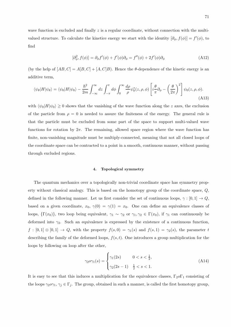
71
wave function is excluded and finally z is a regular coordinate, without connection with the multi-
valued structure. To calculate the kinetice energy we start with the identity [∂φ, f(φ)] = f ′(φ), to
find
[∂2φ, f(φ)] = ∂φf′(φ) + f ′(φ)∂φ = f ′′(φ) + 2f ′(φ)∂φ (A12)
(by the help of [AB,C] = A[B,C] + [A,C]B). Hence the θ-dependence of the kinetic energy is an
additive term,
〈ψθ|H|ψθ〉 = 〈ψ0|H|ψ0〉 −~2
2m
∫ ∞
−∞dz
∫ π
−πdφ
∫ ∞
0
dρ
ρψ∗0(z, ρ, φ)
[
iθ
π∂φ −
(
θ
2π
)2]
ψ0(z, ρ, φ).
(A13)
with 〈ψ0|H|ψ0〉 ≥ 0 shows that the vanishing of the wave function along the z axes, the exclusion
of the particle from ρ = 0 is needed to assure the finiteness of the energy. The general rule is
that the particle must be excluded from some part of the space to support multi-valued wave
functions for rotation by 2π. The remaining, allowed space region where the wave function has
finite, non-vanishing magnitude must be multiply-connected, meaning that not all closed loops of
the coordinate space can be contracted to a point in a smooth, continuous manner, without passing
through excluded regions.
4. Topological symmetry
The quantum mechanics over a topologically non-trivial coordinate space has symmetry prop-
erty without classical analogy. This is based on the homotopy group of the coordinate space, Q,
defined in the following manner. Let us first consider the set of continuous loops, γ : [0, 1] → Q,
based on a given coordinate, x0, γ(0) = γ(1) = x0. One can define an equivalence classes of
loops, {Γ(x0)}, two loop being equivalent, γ1 ∼ γ2 or γ1, γ2 ∈ Γ(x0), if γ1 can continuously be
deformed into γ2. Such an equivalence is expressed by the existence of a continuous function,
f : [0, 1] ⊗ [0, 1] → Q, with the property f(s, 0) = γ1(s) and f(s, 1) = γ2(s), the parameter t
describing the family of the deformed loops, f(s, t). One introduces a group multiplication for the
loops by following on loop after the other,
γ2oγ1(s) =
γ1(2s) 0 < s < 12 ,
γ2(2s− 1) 12 < s < 1.
(A14)
It is easy to see that this induces a multiplication for the equivalence classes, Γ2oΓ1 consisting of
the loops γ2oγ1, γj ∈ Γj. The group, obtained in such a manner, is called the first homotopy group,
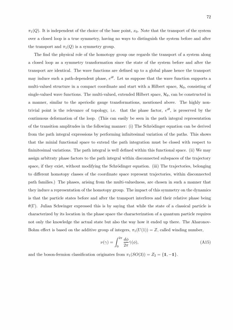
72
π1(Q). It is independent of the choice of the base point, x0. Note that the transport of the system
over a closed loop is a true symmetry, having no ways to distinguish the system before and after
the transport and π1(Q) is a symmetry group.
The find the physical role of the homotopy group one regards the transport of a system along
a closed loop as a symmetry transformation since the state of the system before and after the
transport are identical. The wave functions are defined up to a global phase hence the transport
may induce such a path-dependent phase, eiθ. Let us suppose that the wave function supports a
multi-valued structure in a compact coordinate and start with a Hilbert space, H0, consisting of
single-valued wave functions. The multi-valued, extended Hilbert space, Hθ, can be constructed in
a manner, similar to the aperiodic gauge transformations, mentioned above. The highly non-
trivial point is the relevance of topology, i.e. that the phase factor, eiθ, is preserved by the
continuous deformation of the loop. (This can easily be seen in the path integral representation
of the transition amplitudes in the following manner: (i) The Schrodinger equation can be derived
from the path integral expressions by performing infinitesimal variation of the paths. This shows
that the minial functional space to extend the path integration must be closed with respect to
fininitesimal variations. The path integral is well defined within this functional space. (ii) We may
assign arbitraty phase factors to the path integral within disconnected subspaces of the trajectory
space, if they exist, without modifying the Schrodinger equation. (iii) The trajectories, belonging
to different homotopy classes of the coordinate space represent trajectories, within disconnected
path families.) The phases, arising from the multi-valuedness, are chosen in such a manner that
they induce a representation of the homotopy group. The impact of this symmetry on the dynamics
is that the particle states before and after the transport interferes and their relative phase being
θ(Γ). Julian Schwinger expressed this is by saying that while the state of a classical particle is
characterized by its location in the phase space the characterization of a quantum particle requires
not only the knowledge the actual state but also the way how it ended up there. The Aharonov-
Bohm effect is based on the additive group of integers, π1(U(1)) = Z, called winding number,
ν(γ) =
∫ 2π
0
dφ
2πγ(φ), (A15)
and the boson-fermion classification originates from π1(SO(3)) = Z2 = {11,−11}.