Relative difference contest success function

Theory Dec.DOI 10.1007/s11238-014-9425-4

Relative difference contest success function

Carmen Beviá · Luis C Corchón

© Springer Science+Business Media New York 2014

Abstract In this paper, we present a contest success function (CSF), which is homo-geneous of degree zero and in which the probability of winning the prize depends onthe relative difference of efforts. In a simultaneous game with two players, we presenta necessary and sufficient condition for the existence of a pure strategy Nash equilib-rium. This equilibrium is unique and interior. This condition does not depend on thesize of the valuations as in an absolute difference CSF. We prove that several propertiesof Nash equilibrium with the Tullock CSF still hold in our framework. Finally, weconsider the case of n players, generalize the previous condition and show that thiscondition is sufficient for the existence of a unique interior Nash equilibrium in purestrategies. For some parameter values of our CSF and when all players are identical,equilibrium entails full rent dissipation for any number of players.

Keywords Contest success functions · Contest · Nash equilibrium

JEL Classification C72 · D72 · D74

This paper is dedicated to Gordon Tullock whose insightful work has been inspirational for both authors.We thank Matthias Dahm, Joerg Franke, Magnus Hoffmann, Scott Moser, Guillaume Roger, SantiagoSanchez-Pages, Marco Serena, Anil Yildizparlak, an anonymous referee and the participants of a seminarat the SAET 2012 congress, Brisbane, for comments that substantially improved the quality of the paper.The first author acknowledges financial support from ECO2008-04756 and FEDER, SGR2009-0419 andthe Barcelona GSE research network. The second author acknowledges financial support from ECO2011-25330. Both authors acknowledge the hospitality of the Australian School of Business during the revisionof the paper.

C. Beviá (B)Universitat Autónoma de Barcelona and Barcelona GSE, Barcelona, Spaine-mail: [email protected]

L. C. CorchónUniversidad Carlos III de Madrid, Madrid, Spain

123

C. Beviá, L. C. Corchón

1 Introduction

The concept of a contest success function (CSF) plays a crucial role in the analysisof contests. This function encapsulates how the contest is played and what the con-sequences of the contest are. Thus, the outcome of a contest is highly sensitive to theform of CSF employed.

There are two main families of CSF. The CSF proposed by Tullock (1980) (axiom-atized by Skaperdas (1996)) in which the probabilities of winning the prize depend onrelative efforts, and the difference form proposed by Hirshleifer (1989) (also axioma-tized by Skaperdas (1996) , see, in addition, Baik (1998) and Che and Gale (2000)) inwhich the probabilities of winning the prize depend on the difference between efforts.

Both formulations have properties that one would like to have in an ideal CSF.The Tullock form is homogeneous of degree zero; thus, the units in which effortsare measured do not count. The Hirshleifer form captures “the tremendous advantageof being even just a little stronger than one’s opponent” (Hirshleifer 1991, p. 131).However, this advantage cannot be independent of the size of the conflict. One morebattalion is a great advantage in a battle of two battalions against one but of less helpwhen two hundred battalions fight one hundred and ninety nine. Thus, differencesmust be scaled up to the size of the conflict.

In this paper, we present the Relative Difference CSF (RDCSF) in which the prob-ability of getting the prize depends on the difference between efforts and is alsohomogeneous of degree zero. When there are two players, the RDCSF is an affinefunction of the difference between a player’s effort and the effort of the other player,which is weighted by a positive number and divided by the sum of efforts. When theweight of the effort of the other player and the intercept are zero, we have the TullockCSF; thus, the RDCSF generalizes the latter. The RDCSF is presented in Sect. 2 forthe case of two players.

In Sect. 3, we study a simultaneous move game with two players. We find a necessaryand sufficient condition for the existence of a pure strategy Nash equilibrium . Thisequilibrium is unique, and all players exert a positive effort. This condition is satisfiedwhen the sum of the intercept and the slope of the affine function defining the RDCSFadd up to no more than one (a condition that is always satisfied in the Tullock case).We show that in equilibrium, the player with a higher valuation of the prize regardsefforts as strategic complements, whereas the player with a lower valuation regardsefforts as strategic substitutes1.

In Sect. 4, we study the case of n players. The extension of the CSF presented inSect. 2 to more than two players is not straightforward. First, we have to choose afunctional form that generalizes the CSF to more than two players (there are manyof these forms). However, the main problem is to guarantee that this functional formrepresents probabilities, i.e., yields non-negative values and adds up to one. We solvethis problem by introducing a rationing rule that gives priority to the players with thelargest expenses. Probabilities are assigned until they add up to one. In some cases,a player might be given zero probability of winning the contest despite the fact that

1 This result was shown by Dixit (1987) assuming a difference or a logit CSF (a generalization of theTullock CSF).

123


she is exerting a positive effort, which, of course, cannot happen in equilibrium. Withthis procedure in hand, we show that a Nash equilibrium exists, is unique and that allplayers exert a positive effort.

Our results obtained in Sects. 3 and 4 on the existence of a Nash equilibrium contrastwith those obtained for a Hirshleifer-type CSF where, with linear costs, at most onecontestant exerts a positive effort in any pure strategy Nash equilibrium and a purestrategy Nash equilibrium does not exist when the value of the prize is sufficiently large(see Hirshleifer (1989); Baik (1998) and Che and Gale (2000)). These two propertiesrestrict the range of application of this type of CSF.

In Sect. 5, we present a CSF in which the probability that a player wins the prizeis an affine function of her effort relative to the total effort. 2 At first blush, it mayseem that relative differences do not play a role in this CSF. However, we show thatsuch a CSF is identical to the CSF presented in previous sections. Therefore, we callthe CSF presented in this section the twin CSF. We show that the term reflecting thedifference affects both the intercept and the slope of the twin CSF. An increase in theweight of other players’ efforts in the RDCSF decreases the intercept and increasesthe slope of the twin CSF. Thus, the weight of other players’ efforts in the RDCSF canbe interpreted as a measure of the degree of responsiveness of the winning probabilityto relative efforts.

Finally, Sect. 6 offers some comments about possible extensions of our work.We are only aware of a CSF that depends on differences and that is homogeneous

of degree zero: the Serial Contest proposed by Alcalde and Dahm (2007). However,this CSF does not generalize Tullock’s CSF. A recent paper by Hwang (2012) presentsa CSF that depends on differences and that at the limit, when a parameter tends toone, becomes the Tullock CSF. However, this CSF is not of a difference form andhomogeneous of degree zero at the same time.

2 The relative difference contest success function

We start with the case of two players to gain intuition on the relative CSF. In Sect. 4,we present the generalization for the case of n players.

We motivate our CSF by means of the following properties.Our CSF should be based on a function, denoted by fi (·), which depends on the

difference between weighted efforts G1 and sG2 where s is a positive number. Ifs = 1 the function depends on the difference G1 − G2. We also want our CSF tobe homogeneous of degree zero. A possibility is to write fi ((G1 − sG2)/G j ) as inAlcalde and Dahm (2007) where j could be 1 or 2; however, in this case, we have toredefine the function each time G j is zero. Instead, we divide the difference by theaggregate effort G1 + G2; thus, we have to redefine our CSF only when both effortsare zero. Thus, fi (·) is written as fi ((G1 − sG2)/(G1 + G2)). Next, we take fi (·)to be the simplest possible form, namely, linear. Last, we assume symmetry; thus,the intercept and the slopes of f1(·) and f2(·) are identical. A function with all theseproperties must have the following form:

2 The Tullock CSF is a special case of this CSF when the affine function is linear with unit slope.

123


fi (Gi , G j ) = α + βGi − sG j∑2

k=1 Gk, if

2∑

k=1

Gk �= 0, i, j ∈ {1, 2}, i �= j, (1)

fi (Gi , G j ) = 1

2if

2∑

k=1

Gk = 0, i, j ∈ {1, 2}, i �= j. (2)

with β > 0 to guarantee that fi is increasing in Gi and α ∈ [0, 1] to havefi (sG j , G j ) ∈ [0, 1]. When α = s = 0 and β = 1, we obtain the Tullock CSF.3 Part(2) takes care of the case in which all efforts are zero and is the usual expedient whendefining the Tullock CSF.

In the sequel, we will call the function defined in (1) and (2) the notional CSF. Forf1(·) and f2(·) to be a real CSF, the two properties below must hold.

(a) fi (G) ∈ [0, 1] for i ∈ {1, 2}, and(b)

∑2i=1 fi (G) = 1.

where G = (G1, G2). Conditions (a) and (b) are satisfied in some special cases, i.e.,when α = s = 0 and β = 1, particularly, when the notional CSF is the Tullock CSF.However, in general, we need extra conditions to convert (1)–(2) into a CSF. To takecare of part (a), we define our CSF as min(max( fi (G), 0), 1). This minmax operatoris used by Che and Gale (2000) with the same purpose as us, namely, to guarantee thatthe winning probabilities are between zero and one. To guarantee part (b) above, weadd (1) over all players and find that

2α + β(1 − s) = 1. (3)

Condition (3) also guarantees that G1 = G2 implies p1 = p2, i.e., our notional CSFis symmetric. Note that this condition plus α ∈ [0, 1] implies that −1 ≤ β(1− s) ≤ 1.Now, we are ready to offer our main definition.

Definition 1 The RDCSF for two players is defined as follows:

pi = min(max( fi (Gi , G j ), 0), 1), i, j ∈ {1, 2}, i �= j. (4)

where 2α + β(1 − s) = 1.

We note two things:

1. A more exact description of this CSF would be “Relative Weighted Difference”;however, we chose the shorter name in the hope that this name would not lead toany confusion.

2. When s = 0 (when the RDCSF becomes the Tullock CSF), the CSF in Definition1 is no longer a “Relative Difference” CSF. However, we may assume that s > 0;in this case, the Tullock CSF is the limit case of the RDCSF when s → 0. Wedecided to retain the case s = 0 for simplicity.

3 Actually this form only generalizes the Tullock CSF in ratio form; however, the generalization to thegeneral Tullock CSF is simple, see (35) in the Conclusions.

123


Fig. 1 Winning probability for player 1 as a function of the relative differences (α = 1/2, s = 1)

With the RDCSF, a player making zero effort might win the contest (as it happensin the absolute difference CSF of Che and Gale (2000), see Sect. 5 for examples).

In Fig. 1, we represent the winning probability for player 1 as a function of therelative differences for the case s = 1. In this case, condition (3) does not impose anyrestriction on β. When β = 0, the outcome of the contest does not depend on relativedifferences. When β tends to infinity, RDCSF coincides with the all-pay auction.

3 Equilibrium with two players

In this section, we study the existence and uniqueness of a pure strategy Nash equi-librium of the simultaneous move game with two players. We end the section with theproperties of equilibrium strategies and payoffs.

The RDCSF, denoted by p1(G), p2(G), yields payoff functions πi (G) =pi (G)Vi − Gi , i ∈ {1, 2} where Vi is i’s valuation of the prize. A Nash equilibrium ofthe simultaneous move game is a pair G∗ = (G∗

1, G∗2) such that πi (G∗) ≥ πi (Gi , G∗

j )

j �= i for all Gi , i ∈ {1, 2}.Let us define Yi ≡ Vi

∑2k=1

1Vk

, i ∈ {1, 2}. Note that for both players Yi > 1 andthat for the player with the smallest valuation, say j, Y j ≤ 2. If the valuations of bothplayers are identical, Yi = 2.

To prove the existence of a Nash equilibrium, we need an assumption which makesthe probability of winning not too sensitive to relative differences in efforts. This isbecause, as we saw before, when β is large, the RDCSF approaches the all-pay auctionin which a pure strategy Nash equilibrium does not exist (Hillman and Riley 1989;Baye et al. 1996). Formally, we require that

Yi (α + β) ≥ β(1 + s)

(

2 − 1

Yi

)

, i ∈ {1, 2}. (5)

Note that Assumption (5) is independent of the units of measurement.

123


If players have identical valuations and given (3) (2α + β(1 − s) = 1), condition(5) is 2 ≥ β(1 + s) or α + β ≤ 3/2. If β = 1 and s = α = 0 (the Tullock CSF),condition (5) is Yi + 1/Yi ≥ 2, which always holds. In the Appendix, we show thatAssumption (5) is implied by α + β ≤ 1. Note that, the ratio of valuations is limitedby (5); however, this assumption says nothing about the absolute value of valuationsas in the Hirshleifer-type CSF studied in Baik (1998) and Che and Gale (2000).

The next proposition shows the existence of a pure strategy Nash equilibrium. Theproof is in the appendix.

Proposition 1 Under Assumption (5) there is a unique pure strategy Nash equilibrium,(G∗

1, G∗2), in which both players are active. In equilibrium,

G∗i = β(1 + s)Vi

Yi

(

1 − 1

Yi

)

, i ∈ {1, 2}, (6)

and pi = α + β

(

1 − 1 + s

Yi

)

, i ∈ {1, 2}. (7)

The proof first considers an auxiliary game defined by the notional CSF. We thenshow that using the minmax operator to convert the auxiliary game to a contest doesnot change the equilibrium. This implies that we can study the best reply functions byconsidering the first order conditions of the notional CSF, namely

β(1 + s)G j

(∑2

k=1 Gk)2Vi − 1 = 0, i ∈ {1, 2}. (8)

Note that, contrary to the case in which the CSF is based on absolute differences,the RDCSF yields a pure strategy Nash equilibrium in which both contestants exert apositive effort, even if they value the prize highly. Furthermore, Assumption (5) is notonly sufficient for the existence of an equilibrium, but is also necessary.4 The proof isin the appendix.

Proposition 2 If Assumption (5) does not hold, there is no pure strategy Nash equi-librium.

To build intuition on Propositions 1 and 2, we study the best reply functions in thecase of a common valuation V . From (38), we obtain

Gi (G j ) =√

β(1 + s)G j V − G j , i ∈ {1, 2}. (9)

Equation (9) is the best reply for player i whenever i gets non-negative profits andf (Gi (G j ), G j ) ≤ 1. If profits are positive at (Gi (G j ), G j ), but f (Gi (G j ), G j ) > 1,

then the best reply for player i is to choose Gi such that f (Gi , G j ) = 1. If profits arenegative at (Gi (G j ), G j ), then the best reply for player i is Gi = 0.

4 See Malueg and Yates (2005, 2006) for sufficient conditions for the existence of a Nash equilibriumwhen the CSF is homogeneous of degree zero.

123


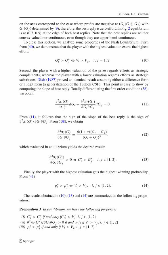
Fig. 2 Best reply functions when V = 1, s = 1, α = 1/2 and β = 1

Fig. 3 Best reply functions when V = 1, s = 1, α = 1/2 and β = 1.5

We draw the best reply of each player for two cases. First, when a pure strategyNash equilibrium exists, and second, when such an equilibrium does not exist. Tosimplify calculations, we take V = 1, α = 1/2, and s = 1. Given Assumption (5),under these parameters a pure strategy Nash equilibrium exists if and only if β ≤ 1.

In the first case, we take β = 1, and in the second case, we take β = 1.5. In Figs. 2and 3, the solid line represents the best reply for player 1 and the dash line the bestreply for player 2. The curvilinear line in both figures corresponds to the part of thebest reply characterized by the first order condition as in (9). The straight line witha positive and finite slope correspond to the case where the best reply is determinedby the probability of winning being equal to 1. Finally, the dashed and the solid lines

123


on the axes correspond to the case where profits are negative at (Gi (G j ), G j ) withGi (G j ) determined by (9); therefore, the best reply is zero effort. In Fig. 2 equilibriumis at (0.5, 0.5) at the edge of both best replies. Note that the best replies are neitherconvex-valued nor continuous, even though they are upper-hemi-continuous.

To close this section, we analyze some properties of the Nash Equilibrium. First,from (40), we demonstrate that the player with the highest valuation exerts the highesteffort:

G∗i > G∗

j ⇔ Vi > Vj , i, j = 1, 2. (10)

Second, the player with a higher valuation of the prize regards efforts as strategiccomplements, whereas the player with a lower valuation regards efforts as strategicsubstitutes. Dixit (1987) proved an identical result assuming either a difference formor a logit form (a generalization of the Tullock CSF). This point is easy to show bycomputing the slope of best reply. Totally differentiating the first order condition (38),we obtain

∂2πi (G)

∂G2i

dGi + ∂2πi (Gi )

∂Gi∂G jdG j = 0. (11)

From (11), it follows that the sign of the slope of the best reply is the sign of∂2πi (G)/∂Gi∂G j . From ( 38), we obtain

∂2πi (G)

∂Gi∂G j= β(1 + s)(Gi − G j )

(Gi + G j )3 , (12)

which evaluated in equilibrium yields the desired result:

∂2πi (G∗)∂Gi∂G j

> 0 ⇔ G∗i > G∗

j , i, j ∈ {1, 2}. (13)

Finally, the player with the highest valuation gets the highest winning probability.From (41)

p∗i > p∗

j ⇔ Vi > Vj , i, j ∈ {1, 2}. (14)

The results obtained in (10), (13) and (14) are summarized in the following propo-sition:

Proposition 3 In equilibrium, we have the following properties

(i) G∗i > G∗

j if and only if Vi > Vj , i, j ∈ {1, 2}(ii) ∂2πi (G∗)/∂Gi∂G j > 0 if and only if Vi > Vj , i, j ∈ {1, 2}

(iii) p∗i > p∗

j if and only if Vi > Vj , i, j ∈ {1, 2}.

123


4 The case of n players

In this section, we study the case of a simultaneous game with n players. First, wegeneralize the CSF defined in Sect. 2. The construction of a CSF for more than twoplayers based on the idea of relative differences requires some extra work with respectto the two-person case because the minmax operator introduced there (see (4)) doesnot guarantee that the sum of the intended probabilities adds up to one.5 We introducean extra device, which guarantees that, under a condition that is a generalization ofassumption (5), a pure strategy Nash Equilibrium exists and is unique.

4.1 The RDCSF in the case of n players.

Let G = (G1, ..., Gn). The notional CSF (1) can be generalized in several ways. Tostay as close as possible to the case of n = 2, we propose the following function:

fi (G) = α + βGi − s

∑j �=i G j

n−1∑nj=1 G j

, i ∈ {1, .., n} ifn∑

j=1

G j �= 0, (15)

fi (G) = 1

nif

n∑

j=1

G j = 0, i ∈ {1, .., n}. (16)

We require that for all G,∑n

i=1 fi (G) = 1. Adding up (15) over players the followingcondition must hold

nα + β(1 − s) = 1. (17)

This condition is a generalization to n players of (3). The Tullock CSF arises whenα = 0, β = 1 and s = 0. Note that the notional CSF is anonymous, wheneverGi = G j , fi (G) = f j (G), but it violates the axiom of Consistency in (Skaperdas(1996), Axiom 4)’s characterization of the general Tullock CSF.6

Based on (15), we define a CSF using the following auxiliary function:

�i (G) = min(max( fi (G), 0), 1). (18)

Unfortunately, when n > 2, the minmax operator does not guarantee that∑

�i (G) =1; thus, an extra construction is needed. In particular, let the players with the largestexpenses be given the probabilities corresponding to (18). Once the probabilities add

5 We note that the difficulties of extending the CSF for more than two players are shared by other CSF likethe difference of Baik (1998) and Che and Gale (2000) or the serial contest of Alcalde and Dahm (2007).6 Consistency requires that the win probability for each player is proportional to the win probability of thesame player in a contest within any subset of players. This axiom is violated when the deleted contestantdoes particularly well/bad against another contestant; thus, deleting a contestant might alter the relativeprobabilities of winning the contest (see Corchón (2007), Example 2.1; see also Sect. 5 for examples ofcontests where this axiom is violated).

123


up to one, the remaining players are given zero probability. To formally introduce theCSF, we need some extra notations. Given G, a type i player is a player that exerciseseffort Gi . Let ki be the number of players of type i, and let li be the last player oftype i.

Definition 2 The RDCSF for any number of players is defined as follows: Given G,order the type of players by decreasing order of Gi . Let m be the type of player suchthat

∑lmj=1 � j (G) ≤ 1 and

∑lm+1j=1 � j (G) > 1. Then,

p j (G) = � j (G), for all j ∈ {1, .., lm}, (19)

pm+1(G) =⎛

⎝1 −lm∑

j=1

� j (G)

⎞

⎠ /(km+1), for all players of type m + 1, and

(20)

ph(G) = 0 for all h ∈ {lm+1 + 1, .., n}. (21)

where nα + β(1 − s) = 1.

We may regard conditions (19), (20), and (21) as a rationing rule: players arerationed depending on their expenditures. Agents with the largest expenses are givenpriority, and their probabilities of winning the contest are given by (18). Agents withless expenses might be given zero probability of winning despite the fact that (18)would recommend a positive probability. This rationing rule reflects the competitiveaspect of the contest by rewarding players who exert more effort.

Note that if G �= (0, .., 0) and 0 ≤ fi (G) ≤ 1 for all i ∈ {1, .., n}, then pi = fi (G),

and if G = (0, .., 0), pi = 1/n for all i ∈ {1, .., n}. For the case of n = 2, the CSF(19) can be written as follows:

pi = �i (G); and p j = 1 − �i (G), (22)

because whenever fi (G) ≤ 0, then f j (G) ≥ 1 (given that condition (17) is satisfied).Therefore, in this case, the extra conditions ( 19), (20), and (21) are not needed.

Remark 1 Despite the fact that we need the rationing rule to define a contest successfunction, in equilibrium, no agent is rationed because if a player j is rationed andG∗

j �= G∗r for any r , this agent j can decrease infinitesimally G∗

j , obtain the prize withthe same probability and increase payoffs. If there are r and j with G∗

r = G∗j , player

j, by increasing infinitesimally G∗j , takes all the probability allocated to r , her cost

only increases infinitesimally and her payoff increases.

4.2 Nash equilibrium with n heterogeneous players

As in Sect. 3, let Yi ≡ Vi∑n

j=11

Vj. To prove the existence of a Nash equilibrium, we

need the following assumption, which is a generalization of Assumption (5):

123


Yi (α + β) ≥ β(n − 1 + s)

(

2 − n − 1

Yi

)

, i ∈ {1, .., n}. (23)

When all players have identical valuations, Assumption (23) collapses in n ≥ β(n −1 + s), which, when either n is sufficiently large or s = 1, is just β ≤ 1. In theAppendix, we show that Assumption (23) is implied by α + β ≤ 1. The latter impliesthat when all players but i exert zero effort, the notional CSF yields a number forplayer i less or equal than one.

To simplify the presentation, we focus on Nash equilibria where all players exerta positive effort. To guarantee the existence of such an equilibrium, we make thefollowing assumption:

Yi > (n − 1), i ∈ {1, .., n}, (24)

which, of course, holds in the symmetric case where Yi = n for all i and when n = 2.An identical assumption guarantees that when the CSF is of the Tullock type, allplayers are active in equilibrium, see Franke et al. (2012), Theorem 2.2. Now we havethe following:

Proposition 4 Under Assumption (23) and Assumption (24), there is a pure strategyNash equilibrium , (G∗

i )ni=1,with all players active. In equilibrium,

G∗i =

(n − 1)β(

1 + sn−1

)Vi

Yi

(

1 − n − 1

Yi

)

, i ∈ {1, .., n}, (25)

and pi = α + β

⎛

⎝1 −(n − 1)

(1 + s

n−1

)

Yi

⎞

⎠ , i ∈ {1, .., n}. (26)

The proof follows the steps of the two players case, see the appendix for details.Proposition (4) implies that, from the point of view of the use of the RDCSF, it

suffices to consider the notional CSF (15). Moreover, equilibrium expenses (25) andwinning probabilities (26) are given by those in the auxiliary game where payoffs aredetermined by the notional CSF.

Note that when all players have identical valuations, V, aggregate equilibriumefforts are

(n − 1 + s)βV

n. (27)

Assumption (23) implies that aggregate effort is less or equal than V . Thus, unlessn = β(n − 1 + s) (which happens if s = β = 1), rents are not fully dissipated, as inthe two-person case. Aggregate effort is minimized when s = 0, which includes theTullock CSF (where in addition α = 0) in which total effort is V/2.

In what follows, we prove that uniqueness of an equilibrium in pure strategies isalso obtained under assumptions (23) and (24). We distinguish two cases that require

123


different proofs. Proposition 5 addresses uniqueness when α+β > 1, and Proposition6 addresses uniqueness when α + β ≤ 1.

Proposition 5 If α + β > 1 there is at most a Nash equilibrium that is interior.

Proposition 6 If Assumption (24) holds and α + β ≤ 1 there is at most a Nashequilibrium that is interior.

Summarizing, Propositions 4, 5 and 6 show that under assumptions (23) and (24),there is a unique equilibrium in pure strategies. In equilibrium, all agents choose apositive effort.

5 A twin CSF

In this section, we motivate our CSF from a different angle. We present several exam-ples of contests in which the Tullock CSF does not appropriately reflect how expensesinfluence winning probabilities. We present a CSF that does appropriately reflect thisinfluence. Furthermore, we prove that this CSF and the relative difference CSF areindeed identical.

Consider the following examples:

1. Political competition: Political parties compete for office. They advertise to influ-ence voters. However, some voters may vote for a certain party irrespective of theamount of advertising (see Skaperdas and Grofman 1995).

2. Competition for audience: Radio/TV stations make expenses to boost the qualityof their programs, and thus the audience. However, some listeners/viewers mayprefer a station irrespective of the expenses of the others because that station betterfits their tastes, i.e., it focuses on Pop music (and not on classical music) or, sitcoms(and not TV shows).

3. Litigation: In a trial in which contenders have conflicting rights, the jury (in theAnglo-Saxon system) or the judge (in the French system) may be opinionated infavor of one of these rights. Thus, even if one of the contenders has only a publicdefender (which is free) and the other hired a very expensive law firm, the formermay win the case.

In all these examples, if a contender has very small (or even zero) expenses, sheretains a non-negligible share of the prize.7 Conversely, contenders making arbitrarilylarge expenses do not win with probability close to one. These examples contradict theTullock CSF where the probability of winning goes to zero (one) when the expensemade by this player goes to zero (infinite). 8

Let us now consider the polar situation in which contestants have to meet certainminimal expenses to have a positive chance of winning.

7 A CSF with this property was presented by Amegashie (2006). However, this CSF is not homogeneousof degree zero.8 The generalized Tullock CSF, namely,

pi = Gαi∑n

j=1 Gαj

123


4 Lobbying: To establish a potentially successful lobby, contestants have to incurfixed costs such as for renting an office, hiring administrative staff, etc.

A simple way of dealing with the situations considered above is to consider thefollowing notional CSF inspired in the Tullock CSF9:

gi (G) = A + BGi

∑nj=1 G j

. (28)

Note that when A > 0 in (28), contestants win the prize with a probability boundedaway from zero even if their expenses are arbitrarily close to zero (Examples 1–2–3above). The case A < 0 corresponds to the case when a fixed expense has to be madeto have a chance to obtain the prize (Example 4 above).10

Now, we note the following:

Remark 2 The notional CSF (28) and the notional relative difference CSF are identical.

Proof Let

fi (G) = α + βGi − s

∑j �=i G j

n−1∑nj=1 G j

. (29)

Adding and subtracting in the numerator Gis

n−1 , we have

fi (G) = α + βGi

(1 + s

n−1

)− s

∑nj=1 G j

n−1∑n

j=1 G j= (30)

= α − sβ

n − 1+ β

Gi

(1 + s

n−1

)

∑nj=1 G j

. (31)

Writing A ≡ α − sβn−1 and B ≡ β(1 + s

n−1 ), (3) can be written as

fi (G) = A + BGi

∑nj=1 G j

. (32)

Note that because α, β and s have to satisfy nα + β(1 − s) = 1, (31) becomes

fi (G) = 1 − α − β

n − 1+ nα + nβ − 1

n − 1

Gi∑n

j=1 G j. (33)

Footnote 8 continuedcan cope with complete lack of flexibility regarding the probability of winning wrt expenses (α = 0) or itassumes certain flexibility (α > 0) but not both at the same time.9 Some extra conditions are needed to convert (28) into a real CSF. Because the purpose of this section isto illustrate the range of application of the relative difference CSF, we will refrain from doing so.10 We keep the CSF symmetric; however, a CSF that fits the examples above even better would be one inwhich the independent terms are different for each contender.

123


From the discussion in the previous sections, we know that α +β cannot be very largefor a Nash equilibrium to exist. In particular, α+β ≤ (n+1)/n is a sufficient conditionfor the existence of a Nash equilibrium when all players are identical. Our twin CSF(32) yields an interpretation of this condition: it requires that fixed costs are negativeor small. Thus, large fixed costs might preclude the existence of a Nash equilibrium. Infact, the sufficient condition for the existence of equilibrium with asymmetric playersis α + β ≤ 1, which precludes the existence of positive fixed costs.

Considering (31), we have

A ≡ 1 − β

n− sβ

n(n − 1), B ≡ β(1 + s

n − 1). (34)

Thus, an increase in s decreases A and increases B, i.e., such an increase, decreases theshare of loyal voters/listeners/viewers who can be persuaded to change vote/listen/viewthrough the appropriate expenses. Thus, the effect of an increase in the weight of otherplayers’ expenses is to make the contest more competitive.

6 Conclusions

In this paper, we have presented a new CSF, the RDCSF, which combines propertiesof the Tullock and the Hirshleifer CSFs. The RDCSF is analytically tractable yieldingclosed form solutions that generalize those of the Tullock CSF. When the valuations ofboth players are not very different, and the impact of relative differences on the winningprobability is not large, all contestants exert a positive effort in a Nash equilibrium.Recall that in the Hirshleifer CSF, this only happens when the value of the prize times,the impact of the absolute differences on the winning probability is less than one.

The RDCSF looks like a mild extension of the Tullock CSF. However, new issuessurface.

1. To convert the notional RDCSF into a RDCSF. In the case of two players, thisconversion is accomplished with the minmax operator as in Che and Gale (2000).However, with more than two players, the minmax operator is not sufficient, andwe have to introduce a full-fledged rationing rule that distributes the availableprobabilities among players.

2. Nash equilibrium does not always exist. In the case of two players, we present anecessary and sufficient condition for the existence of an equilibrium. In the caseof more than two players, we present a sufficient condition for the existence ofequilibrium. We provide conditions that guarantee the uniqueness of the equilib-rium.

A drawback of the RDCSF is that it is not continuous when the aggregate efforttends to zero; however, this is a general property of all homogeneous of degree zeroCSFs (see Corchón (2000)). Our CSF is not differentiable at the points where thenotional CSF and the CSF meet. This is property is shared with the CSF using theminmax operator. Despite the complications arising from these issues, we have shownthat the use of the RDCSF is simple and involves only the consideration of the FOCof the auxiliary game where payoffs are determined by the notional CSF.

123


We hope that the RDCSF can be useful in the analysis of conflicts in which there is anadvantage of being stronger; however, this advantage must be weighted by a measureof how large the conflict is. Because many papers in this area used the Tullock CSF,the use of the RDCSF would provide a generalization of this work. Moreover, from thepoint of view of revenue maximization, the RDCSF provides a simple CSF in which,for some parameters, full rent dissipation occurs for any number of players.

The RDCSF is amenable to certain extensions. A simple extension would be basedon the following notional CSF:

fi (G) = α + βφ(Gi ) − sφ(G j )

∑2j=1 φ(G j )

, i = 1, 2. (35)

with φ(·) concave. It is easy to show that the methods used in this paper suffice toshow the existence of a Nash equilibrium when the CSF is of the (35) form. When aplayer exerts positive effort, the best replies first increase and then decrease as in theCSF analyzed in this paper (a proof of this point is available upon request). Anotherextension would be the consideration of sequential moves. We can show that the mainresults obtained by Dixit (1987), Baik and Shogren (1992) and Leininger (1993) inthis framework also hold with our CSF11.

Finally, an alternative to the RDCSF with n players presented in this paper wouldbe the following form:

fi (G) = α + βGi − s max j �=i G j

∑nj=1 G j

, i ∈ {1, .., n}. (36)

in which we subtract from Gi not the weighted average of the actions of all othercompetitors but only that of the best competitor. When n = 2 or when players areidentical, both formulations yield identical results; however, both formulations differfor more than two different players.

Appendix

Proof of Proposition 1 Let us see first that (0, 0) cannot be an equilibrium. In (0, 0),the payoff for each player is Vi/2. Let ε > 0 be sufficiently close to zero. Supposethat player 1 deviates and increases her effort to ε. Let G = (ε, 0). In this case,f1(G) = α + β, and f2(G) = α − βs. If α + β ≥ 1, given that 2α + β(1 − s) = 1,

then α − βs ≤ 0. Thus, p1 = 1. Therefore, player 1 will win the contest for sure,and her payoff will be V1 − ε, which is greater than V1/2. If f1(G) = α + β < 1,

p1 = α + β. Because 1 = 2α + β(1 − s) ≤ 2α + β < 2α + 2β, α + β > 1/2. Thus,for ε sufficiently close to zero, (α + β)V1 − ε > V1/2, which implies that G1 = ε isa profitable deviation for player 1. Therefore, (0, 0) is not an equilibrium.

11 The formal study of the sequential game with our CSF can be found in the working paper of this paperat http://papers.ssrn.com/sol3/papers.cfm?abstract_id=2017279

123

http://papers.ssrn.com/sol3/papers.cfm?abstract_id=2017279


To prove that there is an equilibrium in which both players are active, consider asimultaneous move auxiliary game with payoffs

π̂i =(

α + βGi − sG j∑2

k=1 Gk

)

Vi − Gi , for all i ∈ {1, 2}. (37)

We show first that, under Assumption (5), the auxiliary game has an interior equilib-rium. Second, we show that this equilibrium of the auxiliary game is also an equilibriumof our game.

The first order conditions associated with the auxiliary game are

β(1 + s)G j

(∑2

k=1 Gk)2Vi − 1 = 0, i ∈ {1, 2}. (38)

We readily see that the second order conditions hold; thus payoffs of i are concave inGi . Adding up all equations in (38) and setting X ≡ ∑2

k=1 Gk , we obtain

X∗ = (1 + s)β∑2

k=11

Vk

. (39)

Plugging (39) in (38), we find that

G∗i = β(1 + s)Vi

Yi

(

1 − 1

Yi

)

, i ∈ {1, 2}. (40)

Because Yi > 1, G∗i > 0. From the definition of the notional CSF, we have

fi (G∗1, G∗

2) = α + β

(

1 − 1 + s

Yi

)

, i ∈ {1, 2}. (41)

Note that fi (G∗1, G∗

2) ≥ 0 if and only if

Yi (α + β) ≥ β(1 + s), i ∈ {1, 2}. (42)

Under Assumption (5), condition (42) always holds. Furthermore, because∑2k=1 fk(G∗

1, G∗2) = 1, fi (G∗

1, G∗2) ≤ 1 for all i ∈ {1, 2}. Profits in equilibrium

amount to

π∗i = Vi

Yi

[

(α + β)Yi − β(1 + s)

(

2 − 1

Yi

)]

, i ∈ {1, 2}. (43)

Assumption (5) implies that profits are non-negative; thus (G∗1, G∗

2) is an equilibriumof the auxiliary game.

Next, we see that G∗ = (G∗1, G∗

2) is also an equilibrium of the original game.Clearly, no player has a profitable deviation Gi such that 0 ≤ fi (Gi , G∗−i ) ≤ 1 because

123


G∗ is an equilibrium of the auxiliary game. In particular, G̃i such that fi (G̃i , G∗−i ) = 1is not a profitable deviation. Thus, a profitable deviation G ′

i can only occur whenfi (G ′

i , G∗−i ) > 1, or fi (G ′i , G∗−i ) < 0. In the first case, because fi is increasing in

Gi , G ′i > G̃i and pi = 1. The payoff at (G ′

i , G∗−i ) is less than the payoff at (G̃i , G∗−i ).

Therefore, G ′i cannot be a profitable deviation. If fi (G ′

i , G∗−i ) < 0, pi = 0 and thepayoff for player i in this deviation is not larger than zero. Thus, this deviation is notprofitable.Finally, we show that there cannot be an equilibrium (G∗

i , 0) with G∗i > 0. If this were

the case, π∗i = (α + β)Vi − G∗

i so G∗i > 0 cannot maximize the payoff of i .

Proof of Proposition 2 We can not have an equilibrium with both players exertinga positive effort because in this case, and given that Assumption (5) does not hold,payoffs would be negative at least for one player. A player will be better off exertingno effort. Thus, if an equilibrium exists, it has to include players exerting zero effort.Suppose G = (Gi , 0). Because Assumption (5) does not hold, it should be the casethat α + β > 1 (otherwise Assumption (5) will hold as we prove in the Appendix).Therefore, fi (G) > 1, which implies that f j (G) < 0 for player j. Thus, pi (Gi , 0) =1. However, for any Gi > 0, player i by decreasing her effort by ε will be better off.Thus, a pure strategy Nash equilibrium does not exist.

Assumption (23) is implied by α + β ≤ 1.Recall that the sufficient condition is

Yi (α + β) ≥ β(n − 1 + s)

(

2 − n − 1

Yi

)

, i ∈ {1, .., n}. (44)

The minimum of the left hand side of (44) is achieved when

Yi = β(n − 1 + s)

α + β,

and the corresponding value of the left hand side of (44) is

−β2(n − 1 + s)2

α + β+ β((n − 1 + s)(n − 1)

Thus, the the left hand side of (44) is always positive if α(n − 1) ≥ sβ, whichconsidering (17) (i.e., nα + β(1 − s) = 1), is α + β ≤ 1.

Proof of Proposition 4 Note first that (0, 0, .., 0) can not be an equilibrium. In(0, ..., 0), the payoff for each player is Vi/n. Let ε > 0 be sufficiently close tozero. Suppose that player i deviates and increases her effort such that now Gi = ε.

Let G = (0, .., ε, .., 0). In this case, fi (G) = α + β. If α + β ≥ 1, given thatnα + β(1 − s) = 1, then α − (βs)/(n − 1) ≤ 0. Thus, pi = 1. Therefore, player iwins the contest for sure, and her payoff will be Vi − ε, which is greater than Vi/n. Iffi (G) = α +β < 1, pi = α +β. Because 1 = nα +β(1 − s) ≤ nα +β < nα + nβ,

α + β > 1/n, for ε sufficiently close to zero, (α + β)Vi − ε > Vi/n.

123


To prove that there is an equilibrium where all players are active, consider a simul-taneous move auxiliary game with payoffs

π̂i =⎛

⎝α + βGi − s

∑j �=i G j

n−1∑nj=1 G j

⎞

⎠ Vi − Gi , i ∈ {1, .., n}. (45)

We show first that, under assumptions (23) and (24), the auxiliary game has an interiorequilibrium. Second, we show that this equilibrium of the auxiliary game is also anequilibrium of our game.

The first order conditions associated with the auxiliary game are

β

∑j �=i G j (1 + s

n−1 )(∑n

j=1 G j

)2 Vi − 1 = 0, i ∈ {1, .., n}. (46)

We readily see that the second order conditions hold; thus, payoffs of i are concave inGi .

Write Eq. (46) as follows:

∑j �=i G j

(∑n

j=1 G j )2= 1

βVi

(1 + s

n−1

) . (47)

Adding up the equations in (47) over all players and simplifying we obtain

n∑

j=1

G j =(n − 1)β

(1 + s

n−1

)

∑nj=1

1Vj

. (48)

Realizing that (47) can be written as

∑nj=1 G j − Gi

(∑nj=1 G j

)2 = 1

βVi

(1 + s

n−1

) , (49)

and considering (48), we obtain

G∗i =

(n − 1)β(

1 + sn−1

)Vi

Yi

(

1 − n − 1

Yi

)

, i ∈ {1, .., n}. (50)

Because Assumption (24) requires Yi > n − 1, for all i ∈ {1, .., n}, G∗i ≥ 0.

123


From the definition of the notional CSF fi , we have

fi (G∗) = α + β

G∗i

(1 + s

n−1

)− s

∑nj=1 G∗

jn−1

∑nj=1 G∗

j= (51)

= α + βG∗

i∑nj=1 G∗

j

(

1 + s

n − 1

)

− sβ

n − 1. (52)

Considering (49), we have

G∗i∑n

j=1 G∗j

= 1 − (n − 1)

Yi, (53)

and we obtain

fi (G∗) = α + β

(

1 − (n − 1)

Yi

)(

1 + s

n − 1

)

− sβ

n − 1(54)

= α + β

⎛

⎝1 −(n − 1)

(1 + s

n−1

)

Yi

⎞

⎠ . (55)

Note that fi (G∗) ≥ 0 if and only if (α + β)Yi ≥ β(n − 1)(1 + sn−1 ). However,

given Assumptions (23) and ( 24), this condition always hold. Furthermore, because∑ni=1 fi (G) = 1, we have fi (G∗) ≤ 1.Finally, profits in equilibrium amount to

π∗i =

(

α+β

(

1− (n−1)(1+ sn−1 )

Yi

))

Vi −(n−1) β

(1+ s

n−1

)Vi

Yi

(

1− n−1

Yi

)

, (56)

which can be rewritten as follows:

π∗i = (α + β) Vi − β(n − 1)

(

1 + s

n − 1

)Vi

Yi−

(n − 1)β(

1 + sn−1

)Vi

Yi

(

1 − n − 1

Yi

)

,

(57)

π∗i = Vi

Yi((α + β)Yi − β(n − 1)(1 + s

n − 1) − (n − 1)β

(

1 + s

n − 1

) (

1 − n − 1

Yi

)

,

(58)

π∗i = Vi

Yi

(

(α + β)Yi − β(n − 1)

(

1 + s

n − 1

) (

2 − n − 1

Yi

))

. (59)

Assumption (23) implies that profits are non-negative; thus, G∗ = (G∗1, .., G∗

n) is anequilibrium of the auxiliary game. Let us finally see that G∗ is also an equilibriumof the original game. Clearly, no player has a profitable deviation Gi such that 0 ≤fi (Gi , G∗−i ) ≤ 1 because G∗ is an equilibrium of the auxiliary game. In particular, G̃i

123


such that fi (G̃i , G∗−i ) = 1 is not a profitable deviation. Thus, a profitable deviation G ′i

can only occur when fi (G ′i , G∗−i ) > 1, or fi (G ′

i , G∗−i ) < 0. In the first case, becausefi is increasing in Gi , G ′

i > G∗i .Furthermore, because player i has increased her effort,

the f j of the other players is reduced; thus, f j (G ′i , G∗−i ) ≤ f j (G∗) ≤ 1. Therefore,

by the rationing rule, pi = 1. Thus, payoffs at (G ′i , G∗−i ) are less than payoffs at

(G̃i , G∗−i ). Therefore, G ′i can not be a profitable deviation. If fi (G ′

i , G∗−i ) < 0, pi =0; then, the payoff for player i in this deviation cannot be greater than zero. Thus, thisdeviation is not profitable.

Proof of Proposition 5 Suppose that there is a Nash equilibrium with G∗i = 0 for

some i . Then,

pi = α − βs

n − 1= −α − β + 1

n − 1< 0. (60)

Because probabilities add up to one, pi < 0 for some i implies that some active agent,say j , is rationed. However, we already know that in equilibrium no agent can berationed.

We now tackle the case of α +β ≤ 1. A coalition C is a subset of the set of players.Let c be the number of players in coalition C . Consider the following condition:

For any coalition C and player i /∈ C , Vi

∑

j∈C

1

Vj> c − 1. (61)

Lemma 1 shows that condition (61) is always satisfied whenever Assumption (24)holds.

Lemma 1 If Assumption (24) holds, then Vi∑

j∈C1

Vj> c − 1 for any coalition C

and player i /∈ C.

Proof Suppose that condition (61) does not hold. Then, there is a coalition C and aplayer i /∈ C such that Vi

∑j∈C

1Vj

≤ c − 1. In particular, for any player k /∈ C such

that Vk ≤ Vi , Vk∑

j∈C1

Vj≤ c − 1. Let kmin /∈ C be such that Vkmin ≤ Vk for all

k /∈ C. Let us see that Ykmin ≤ n − 1, in contradiction with Assumption ( 24). Giventhat Ykmin = Vkmin

∑nj=1

1Vj

, we can rewrite Ykmin as:

Ykmin = Vkmin

∑

j∈C

1

Vj+ Vkmin

∑

k /∈C

1

Vk. (62)

Given that Vkmin

∑j∈C

1Vj

≤ c − 1, and Vkmin

∑k /∈C

1Vk

≤ n − c, Ykmin ≤ n − 1. ��Proof of Proposition 6 Suppose we have a Nash equilibrium in which only players1, 2, ..., k are active. First we show that player i = k + 1, ....n is not rationed. Indeed

pi = α − βs

n − 1= 1 − α − β

n − 1≥ 0. (63)

123


Thus, player i maximizes, at least in a neighborhood of the Nash equilibrium, overthe notional CSF. The FOC of payoff maximization for i is

∂πi

∂Gi= β

(1 + s

n−1

)

∑kj=1 G j

Vi − 1. (64)

Now computing the expenses made by active players, we see that

k∑

j=1

G j = β(k − 1)

(1 + s

n−1

)

∑kj=1

1Vj

; (65)

thus,

∂πi

∂Gi=

Vi∑k

j=11

Vj

k − 1− 1 (66)

and applying condition (61), we obtain

∂πi

∂Gi>

k − 1

k − 1− 1 = 0, (67)

which contradicts that the best reply of i is zero.

References

Alcalde, J., & Dahm, M. (2007). Tullock and Hirshleifer: A meeting of the minds. Review of EconomicDesign, 11(2), 101–124.

Amegashie, J. A. (2006). A contest success function with a tractable noise parameter. Public Choice, 126,135–144.

Baik, K. H. (1998). Difference-form contest success functions and effort level in contests. European Journalof Political Economy, 14, 685–701.

Baik, K. H., & Shogren, J. F. (1992). Strategic behavior in contests: Comment. American Economic Review,82(1), 359–362.

Baye, M., Kovenock, D., & de Vries, C. G. (1996). The all-pay auction with complete information. EconomicTheory, 8, 291–305.

Corchón, L. (2000). On the allocative effects of rent-seeking. Journal of Public Economic Theory, 2(4),483–491.

Corchón, L. (2007). The theory of contests: a survey. Review of Economic Design, 11, 69–100.Che, Y.-K., & Gale, I. (2000). Difference-form contests and the robustness of all-pay auctions. Games and

Economic Behavior, 30, 22–43.Dixit, A. (1987). Strategic behavior in contests. American Economic Review, 77(5), 891–898.Franke J., C. Kanzow, W. Leininger & A. Schwartz (2012). Effort maximization in asymmetric contests

games with heterogeneous contestants. Economic Theory, forthcoming.Hillman, A. L., & Riley, J. G. (1989). Politically contestable rents and transfers. Economics and Politics,

1, 17–39.Hirshleifer, J. (1989). Conflict and rent-seeking success functions: Ratio versus difference models of relative

success. Public Choice, 63, 101–112.Hirshleifer J. (1991). The technology of conflict as an economic activity”. The American Economic Review,

81, 2, Papers and Proceedings, pp. 130–134.

123


Hwang, S.-H. (2012). Technology of military conflict, military spending, and war. Journal of Public Eco-nomics, 96, 226–236.

Leininger, W. (1993). More efficient ent-seeking - A Munchhausen solution. Public Choice, 75, 43–62.Malueg, D., & Yates, A. (2005). Equilibria and comparative statics in two-player contests. European Journal

of Political Economy, 21(3), 738–752.Malueg, D., & Yates, A. (2006). Equilibria in rent-seeking contests with homogeneous success functions.

Economic Theory, 27, 719–727.Skaperdas, S., & Grofman, B. (1995). Modeling negative campaigning. The American Political Science

Review, 89(1), 49–61.Skaperdas, S. (1996). Contest success functions. Economic Theory, 7, 283–290.Tullock, G. (1980). Efficient rent-seeking. In J. M. Buchanan, R. D. Tollison, & G. Tullock (Eds.), Towards

a theory of a rent-seeking society (pp. 97–112). College Station: Texas A and M University Press.

123

Documents

Relative difference contest success function