Bank of Canada staff working papers provide a forum for staff to publish work-in-progress research independently from the Bank’s Governing Council. This research may support or challenge prevailing policy orthodoxy. Therefore, the views expressed in this paper are solely those of the authors and may differ from official Bank of Canada views. No responsibility for them should be attributed to the Bank.

www.bank-banque-canada.ca

Staff Working Paper/Document de travail du personnel 2016-33

Relationships in the Interbank Market

by Jonathan Chiu and Cyril Monnet

2

Bank of Canada Staff Working Paper 2016-33

July 2016

Relationships in the Interbank Market

by

Jonathan Chiu1 and Cyril Monnet2

1Victoria University of Wellington and Funds Management and Banking Department

Bank of Canada Ottawa, Ontario, Canada K1A 0G9

Jonathan.Chiu@vuw.ac.nz 2University of Bern, Study Center Gerzensee

Swiss National Bank cyril.monnet@vwi.unibe.ch

ISSN 1701-9397 © 2016 Bank of Canada

ii

Acknowledgements

We thank Morten Bech and Marie Hoerova for many useful conversations. We thank

Luis Araujo, Todd Keister, Thomas Nellen, Peter Norman, Guillaume Rocheteau,

Alberto Trejos, Pierre-Olivier Weill, Randall Wright, Shengxing Zhang, and audiences at

Queen’s University; the University of Helsinki; the Vienna Macro Workshop; the

Summer Money, Banking and Liquidity Workshop at the Chicago Fed; the Norges Bank;

the Riksbank; and the second African Search and Matching Workshop for useful

comments.

The views expressed here are those of the authors and do not necessarily reflect the

position of the Bank of Canada or the Swiss National Bank.

iii

Abstract

The market for central bank reserves is mainly over-the-counter and exhibits a core-periphery

network structure. This paper develops a model of relationship lending in the unsecured interbank

market. In equilibrium, a tiered lending network arises endogenously as banks choose to build

relationships to insure against liquidity shocks and to economize on the cost to trade in the

interbank market. Relationships matter for banks’ bidding strategies at the central bank auction

and introduce a relationship premium that can significantly distort the observed overnight rate.

For example, it can explain some anomalies in the level of interest rates—namely, that banks

sometimes trade above (below) the central bank’s lending (deposit) rate. The model also helps to

explain how monetary policy affects the network structure of the interbank market and its

functioning, and how the market responds dynamically to an exit from the floor system. We also

use the model to discuss the potential effects of bilateral exposure limits on relationship lending.

JEL Codes: E4, E5

Bank topics: Interest rates; Monetary policy implementation; Transmission of monetary

policy

Résumé

Le marché des réserves de banques centrales est, dans la plupart des cas, un marché de gré à gré

dont la structure de réseau est de type « centre-périphérie ». Les auteurs modélisent les relations

contractuelles de long terme dans le marché des prêts interbancaires non garantis. Les banques

choisissent d’établir des relations pour se protéger contre des chocs de liquidité et économiser les

coûts des opérations de marché. En situation d’équilibre, un réseau de prêt par paliers est donc

généré de façon endogène. Les relations interbancaires sont importantes pour comprendre les

stratégies de soumission des banques dans le cadre des processus d’adjudication des réserves des

banques centrales. Par ailleurs, les banques en relation incorporent une prime de relation dans les

taux qu’elles négocient, ce qui peut fausser le taux de refinancement à un jour. Ces primes

peuvent, par exemple, expliquer certaines anomalies du niveau des taux d’intérêt – à savoir, le fait

que les banques pratiquent parfois des taux supérieurs aux taux d’escompte des banques centrales

ou inférieurs aux taux de rémunération des dépôts de ces dernières. Le modèle aide également à

expliquer l’influence qu’exerce la politique monétaire sur la structure de réseau et le

fonctionnement du marché des prêts interbancaires ainsi que la réaction dynamique des marchés

lorsque les banques centrales mettront fin à leurs politiques monétaires non conventionnelles. Les

auteurs utilisent aussi le modèle pour analyser les effets des nouvelles réglementations limitant

l’exposition au risque de crédit sur les relations bancaires de long terme.

Classification JEL : E4, E5

Classification de la Banque : Taux d’intérêt, Mise en œuvre de la politique monétaire,

Transmission de la politique monétaire

iv

Non-Technical Summary

Major central banks now implement monetary policy by using a corridor/channel system to

influence interest rates in the interbank market. Contrary to popular belief, the interbank market is

far from being the epitome of a perfectly competitive market. Instead, it is mainly over-the-

counter and exhibits a core-periphery network structure.

This paper develops a model of relationship lending in the unsecured interbank market. In

equilibrium, a tiered lending network arises endogenously as banks choose to build relationships

to insure against liquidity shocks and to economize on the cost to trade in the interbank market.

Relationships matter for banks’ bidding strategies at the central bank auction. They also introduce

a relationship premium that can significantly distort the observed overnight rate. For example,

relationships can explain some anomalies in the level of interest rates—namely, that banks

sometimes trade above (or below) the central bank’s lending (deposit) rate.

A lesson for policy-makers is that trades outside the corridor are consistent with a well-

functioning interbank market, even when all banks have access to the facilities. Thus, the central

bank has no need to worry about eliminating deviations due to long-term relationships. We

should be careful, however, in interpreting the interbank market rate as a reference for the

overnight cost of liquidity because it may also incorporate a relationship premium, which at times

can significantly distort the observed overnight rate.

The model also helps with our understanding of how monetary policy affects the network

structure of the interbank market and its functioning, as well as how the market responds

dynamically to an exit from the floor system. Another way we use the model is to discuss the

potential effects of bilateral exposure limits on relationship lending.

1 Introduction

Major central banks implement monetary policy by targeting the overnight rate in

the unsecured segment of the interbank market for reserves – the very short-term rate

on the yield curve. The textbook principles of monetary policy implementation are

intuitive: Each bank holds a reserve account at the central bank. Over the course of

a normal business day, this account is subject to shocks due to the banks’ payment

inflows or outflows. Banks seek to manage their account balance to satisfy some

forms of reserve requirements.1 The central bank manages the supply of reserves by

conducting auctions or open market operations. By changing the supply of reserves,

it influences the interest rate at which banks borrow or lend reserves in the interbank

market, and, as a consequence, the marginal cost of making loans to businesses and

individuals.2 In recent years, many major central banks have refined this system by

offering two facilities: In addition to auctioning reserves, the central bank stands

ready to lend reserves at a penalty rate – the lending rate – if banks end up short

of reserves. Symmetrically, banks can earn an interest rate – the deposit rate – if

they end up holding reserves in excess of the requirement. As a consequence the

interbank rate should stay within the bands of the corridor defined by the lending

and the deposit rates. This is known as the “corridor system” for monetary policy

implementation.

The reality is more complex than this basic narrative. On many occasions, central

banks overestimated the demand for liquidity needed for banks to satisfy their reserve

requirements (see for example European Central Bank, 2002). Bowman, Gagnon,

and Leahy (2010) and others report that in many jurisdictions with large excess

reserves, banks have been trading below the deposit rate (supposedly the floor of

1The minimum reserve requirement can be either positive (e.g., in the United States) or zero(e.g., in Canada).

2For example, in normal circumstances, the European Central Bank conducts weekly auctions,while the Fed conducts repos with its primary dealers. Tha Bank of Canada conducts open marketopeations and also auctions settlement balances.

2

the corridor).3 It is also well known that banks sometimes trade above the lending

rate (supposedly the ceiling of the corridor). This challenges the basic intuition that

simple arbitrage would maintain the rates within the bands of the corridor. At a

time when central banks are thinking of exiting quantitative easing policies, we may

wonder whether these observations are symptomatic of a dysfunctional interbank

market that will hamper exit, or if they are “natural” phenomena with little relevance

for the conduct of monetary policy during the exit stage.

Contrary to folk belief, the interbank market is very far from being the epitome

of the Walrasian market. For example, Figure 1 illustrates that a large share of the

transactions in the European (unsecured) interbank market is made over-the-counter

(OTC). Also, many banks maintain long-term relationships and they trade with just

a few banks, sometimes only one, or they directly access the central bank facilities

without even trading with another bank. We review the evidence below, but these

facts are now well accepted.

In this paper, we analyze the effects of long-term trading relationships and mon-

3Bowman, Gagnon and Leahy (2010) review the experience of eight major central banks andreport that the deposit rates on reserve do not always provide a lower bound for short-term marketrates. In particular, the (weighted) average of overnight market rates for reserve balances sometimesstayed below the deposit rate during the recent financial crisis, when reserve balances were abundantand the central bank moved its overnight target towards the deposit rate on reserves. In somecountries, a potential explanation for this puzzling observation is that some participants in themoney market cannot earn interest on their deposits at the central bank (e.g., GSEs in the UnitedStates). In some other cases, there is no clear institutional feature that can explain why the averageovernight rate stayed below the floor. For example, according to the above study, in Japan, “[t]heuncollateralized overnight call rate is similar to the federal funds rate, in that it is a daily weightedaverage of transactions in the uncollateralized overnight market. Participants in the market includedomestic city, regional, and trust banks, foreign banks, securities companies, and other firms dealingin Japanese money markets. All of the economically important participants active in the call marketare also eligible to participate in the deposit facility...the overnight call rate has occasionally fallenbelow the Bank of Japan’s deposit rate in the period since November 2008, but never by more than2 basis points.” Similarly, in Canada, there is anecdotal evidence that some banks occasionally lentand borrowed at rates below the floor during the crisis period, even though they had direct accessto central bank deposit facilities. Concerning the explanation for these negative spreads in Canada,some practitioners argued that banks lent below the floor due to concerns about their reputationand relationship with other banks in the market (see Lascelles, 2009).

3

Figure 1: Trading structure of unsecured transactions in the European interbankmarket (Source: ECB, 2013)

etary policy on bidding behavior, interbank trading volume and rates, the network

structure of the interbank market and its functioning. We show that modeling rela-

tionships matters for both individual and aggregate demand for liquidity. Relation-

ships can explain why banks trade below the deposit rate or above the lending rate.

Our analysis also sheds light on the effect of monetary policy on the network struc-

ture. In particular, we show that the current accommodative monetary policy stance

lowers the value of building and maintaining relationships, so that in steady state,

no or few relationships exist. Interestingly, this is what some central bankers have

been pointing out, and it arises endogenously from our model.4 Moreover, relation-

4Bech et al. (2014) find significant changes in lending patterns following the implementation ofthe interest on excess reserves policy by the Federal Reserve on October 9, 2008. Also, Klee andStebunovsy (2013) report a large decline in fed funds volume in the second quarter of 2012, whileBeltran, Bolotnyy, and Klee (2015) find that “many of the smaller lenders reduced their lending tothe larger institutions in the core of the network (...) the federal funds network began to contractrapidly and change dramatically in structure after the Lehman bankruptcy in the fall of 2008.The number of participating banks and transactions plummeted, as did overall dollar volume.”Furthermore they show that “there was a sharp contraction in the number of links in the networkduring the last quarter of 2008 (...) Also, there was a sizable increase in the average dollar volumetransacted per link, which (...) is largely driven by the exit of many of the smaller banks from the

4

ships also matter for the effects of future policy changes. For example, we show how

the interbank network responds dynamically to an exit from the floor system. We

also discuss the potential effects on relationship lending of the regulation on bilateral

exposure which will come into force in 2019.

We model the corridor system for monetary policy implementation under zero

reserve requirements.5 At the beginning of each day, banks can bid for central bank

reserves at the policy rate set by the central bank. This is akin to a tender with

full allotment, like the one the European Central Bank has been operating since

2008. Once they obtain reserves at the tender, banks face a shock to their reserves

holdings. To meet their reserve requirement, banks in a deficit position can borrow

at the central bank’s lending facility at iℓ, and those in a surplus position can deposit

their reserves at the deposit facility to earn id. A positive spread between iℓ and id

gives banks incentives to trade reserves directly with each other. These trades can

be conducted either in the core interbank market where banks can trade with many

different counterparties, or at the periphery of the core market by banks with pre-

established relationships. Some banks (that we call S for “small”) have to pay a

cost to access the core market, while others (that we call L for “large”) can access

it freely.6 In addition, banks can trade reserves with their long-term partners in

the relationship-lending market. Within a relationship, the L bank can provide

intermediation service to S by accessing the core market on its behalf; the S bank

saves on the access cost, and the large bank extracts some rents from providing this

service. Furthermore, a relationship allows long-term partners to trade repeatedly

market.”5Setting the minimum reserve requirement at zero is just a normalization. Our finding does not

rely on this assumption.6For example, small banks usually do not have a liquidity manager and so their opportunity

cost of accessing the core market is high. Hence, small banks will only enter the core market iftheir gains from trade are sufficiently large. Also, “small” and “large” are merely labels for bankswith high and low participation costs. We will show that, in equilibrium, low-cost banks will tradelarger volume than high-cost banks in the interbank market, hence justifying the labels “large” and“small.”

5

over time without the need to search for a new counterparty everyday. However,

relationships can end for exogenous or endogenous reasons. In that case, banks can

search for another long-term partner to build a new relationship.

Within this framework, the corridor can be “soft,” i.e., equilibrium interbank

rates can be below id or above iℓ, when trading frictions are present, even though

small banks can access the deposit/lending facilities at no cost. In other words, it

seems that arbitrage opportunities exist. The intuition is clear: small banks value

long-term relationships, as they provide liquidity insurance and save them the cost

of accessing the core market. As a result, they are willing to temporarily lower their

surplus from trading a loan as long as the long-term gains from keeping a relationship

outweigh the short-term loss. This gives rise to what we call a relationship premium.7

Specifically we show that S banks with surplus reserves agree to lend at a rate below

id, when this helps them keep their relationship. Symmetrically, S banks that need

reserves may end up paying a rate above iℓ. Therefore, in equilibrium, some banks

trade below the floor or above the ceiling of the corridor. On the surface, there seems

to be unexploited arbitrage opportunities. There is none really: S banks are only

willing to trade at a rate outside the corridor for small loans with their long-term

partners, but not for large loans or with other counterparties.

Furthermore, our model implies that the soft floor depends on aggregate liquidity

conditions: It is more likely when there is a large aggregate liquidity surplus or deficit.

A lesson for policy-makers is that trades outside the corridor are consistent with a

well-functioning interbank market, even when all banks have access to the facilities.

Thus, the central bank has no need to worry too much about eliminating deviations

due to long-term relationships. However, one should be careful in interpreting the

interbank market rate as a reference for the overnight cost of liquidity, because it

7This implication is also consistent with the finding by Ashcraft and Duffie (2007) that “[t]herate negotiated is higher for lenders who are more active in the federal funds market relative to theborrower. Likewise, if the borrower is more active in the market than the lender, the rate negotiatedis lower, other things equal.”

6

may also incorporate a relationship premium, which at times can significantly distort

the observed overnight rate.

Our work is also one of the first to attempt to explain the network structure of the

interbank market and its endogenous response to a change in monetary policy. The

network structure that emerges endogenously resembles the core-periphery structure

we observe in the data, where most of the trading activities are due to a number of

banks that appear to intermediate the trades of others. We show that as monetary

policy becomes more accommodative, banks have little gains from their relationships:

Since reserves are cheap, they have enough reserves to satisfy their requirements

under most circumstances and the gains from building relationships and conducting

relationship trades become small. The tiered network structure will then slowly

vanish, as banks are hit by exogenous separation shocks. As the central bank gives

up its accommodative stance, we show that the path to the new steady state is not

necessarily monotonic: S banks may have a large incentive to search for a relationship

early on, and the high success rate explains why S banks can reduce their search

effort below its steady-state level.

Literature

Figure 2 shows the network of the federal funds market as shown by Bech and Atalay

(2010) for September 29, 2006. The market has a core-periphery network structure

(or tiered structure) where some banks in the periphery only trade with one bank,

while the latter might trade with many others.8 Bech and Atalay (2010) point out

that, in the US interbank market, “[t]here are two methods for buying and selling

8Sept. 29 2006 was the last day of the third quarter. Bech and Atalay report that a total of479 banks were active in the market that day. The largest bank in terms of fed funds value tradedis located at the center of the graph. The 165 banks that did business with the center bank lie onthe first outer circle. The second outer circle consists of the 271 banks that did business with thebanks in the first circle, but that did no business with the center bank. The remaining dots arethe 42 banks that were more than two links away from the center. Two banks did business onlybetween themselves. Large-value links are in yellow and small-value links are in red.

7

federal funds. Depository institutions can either trade directly with each other or

use the services of a broker. ... In the direct trading segment, transactions commonly

consist of sales by small-to-medium sized banks to larger banks and often take place

on a recurring basis. The rate is set in reference to the prevailing rate in the brokered

market. In the brokered segment, participation is mostly confined to larger banks

acting on their own or a customers behalf.”

Figure 2: Network structure of the fed funds market (Bech and Atalay, 2010)

Stigum and Crescenzi (2007, Ch. 12) also report anecdotal evidence of the tiered

structure of the fed funds market. In particular, they report that

“[i]n the fed funds market now, regional banks buy up funds from even

tiny banks, use what they need, and resell the remainder in round lots in

the New York market. Thus, the fed funds market resembles a river with

tributaries: money is collected in many places and then flows through

various channels into the New York market. In essence, the nation’s

smaller banks are the suppliers of fed funds, and the larger bankers are

the buyers.”

Also

8

“[t]o cultivate correspondents that will sell funds to them, large banks

stand ready to buy whatever sums these banks offer, whether they need all

these funds or not. If they get more funds than they need, they sell off the

surplus in the brokers market. Also, they will sell to their correspondents

if the correspondents need funds, but that occurs infrequently. As a

funding officer of a large bank noted, ‘We do feel the need to sell to

our correspondents, but we would not have cultivated them unless we

felt that they would be selling to us 99% of the time. On the occasional

Wednesday when they need $ 100,000 or $ 10 million, OK. Then we would

fill their need before we would fill our own.’”

Elsewhere, using Bundesbank data on bilateral interbank exposures among 1,800

banks, Brauning and Fecht (2012) and Craig and Von Peter (2014) find strong evi-

dence of tiering in the German banking system. Using UK data Vila et. al. (2010)

also report the existence of a core of highly connected banks alongside a periphery.

Of course, this has important consequences on rates. As Stigum and Crescenzi (2007)

note,

“A few big banks, however, still see a potential arbitrage, ‘trading profits,’

in selling off funds purchased from smaller banks and attempt to profit

from it to reduce their effective cost of funds. Also a few tend to bid

low to their correspondents. Said a trader typical of the latter attitude,

‘We have a good name in the market, so I often underbid the market by

1/16.”

Our paper is related to the literature on the interbank market and monetary policy

implementation, to the growing literature on financial networks, and to the literature

on OTC markets. The first literature on the interbank market includes Poole (1968),

Hamilton (1996), Berentsen and Monnet (2006), Berentsen, Marchesiani, and Waller

(2014), Bech and Klee (2011), Afonso and Lagos (2014), and Afonso, Kovner and

9

Schoar (2012), among others. See also Bech and Keister (2012) for an interesting ap-

plication of the Poole (1968) model to reserve management with a liquidity coverage

ratio requirement. While Afonso, Kovner, and Schoar (2012) show some evidence of

long-term relationship in the interbank market, none of the papers above accounts

for it. Rather, they all treat banks as anonymous agents conducting random, “spot”

trades. So our paper is the first to study the effect of long-term relationship on rates.

Based on private information, Ennis and Weinberg (2013) explain why some banks

can borrow at a rate above the central bank’s lending rate. The early literature

on financial networks is mostly motivated by understanding financial fragility and

has been covered in Allen and Babus (2009); see also Jackson (2010). It includes

Allen and Gale (2000) who study whether some banks’ networks are more prone to

contagion than others. Also, Leitner (2005) studies the optimality of linkages, mo-

tivated by the desirability of mutual insurance when banks can fail; while Gofman

(2011) and Babus (2013) analyze the emergence and efficiency of intermediaries in

OTC markets. In a recent calibration exercise, Gofman (2014) finds that it is sub-

optimal to limit banks’ interdependencies in the interbank market. Elliott, Golub,

and Jackson (2014) apply network theory to financial contagion through net worth

shocks. Finally, the literature on OTC markets includes Duffie, Garleanu, and Ped-

ersen (2005), and Lagos and Rocheteau (2006), among many others.9 Within this

literature, Chang and Zhang (2015) study network formation in asset markets based

on heterogeneous liquidity preferences.

There is a large empirical literature on the interbank market, and we already

mentioned a few papers. Furfine (1999) proposes a methodology to extract fed

funds transactions from payments data, and Armantier and Copeland (2012) test

the methodology. Afonso, Kovner and Shoar (2011) study the fed funds market in

times of stress. The two papers closest to ours are perhaps the empirical study of

9See also Afonso and Lagos (2014); Li, Rocheteau and Weill (2012); Lagos, Rocheteau, and Weill(2011); and Rocheteau and Wright (2013).

10

Brauning and Fecht (2012) and the theoretical paper of Blasques, Brauning, and

van Lelyveld (2015). Brauning and Fecht suggest a theory of relationship lending

based on private information, as proposed by Rajan (1992). In good times, banks

extract an informational rent, thus explaining why the relationship lending rates are

usually higher than the average rate in normal times. In bad times, a lending bank

knows whether the borrower is close to failure and it is willing to offer a discount in

order to keep the bank afloat. This argument fails to recognize that in bad times,

some borrowers may not be close to failure and the rent that can be extracted from

a relationship lender can be even higher then. Moreover, the size of discount in-

volved in these loans is usually not an amount significant enough to matter for the

survival of a borrowing bank. Although we do not want to minimize the role of

private information, we argue that the simple threat of terminating the relationship

can also yield to interbank rate discounts. Blasques, Brauning, and van Lelyveld

(2015) study a dynamic network model of the unsecured interbank market based on

peer monitoring. However, they do not study the impact of the supply of reserves

on the structure of the network, or explain why interest rates can fall outside of the

corridor.

Section 2 describes the environment. For simplicity, we start with a basic model

where the core interbank market is competitive and frictionless. Sections 3 and 4

characterize the equilibrium. In Section 5, we analyze the qualitative implications

of this basic model. Section 6 then extends the model to incorporate an OTC inter-

bank market and reports some quantitative implications of the extended model. We

conclude in Section 7.

2 Model

We model the daily reserve management problem of banks in a corridor system. To

study relationships and to determine their equilibrium values, we consider an infinite

11

horizon model with discrete time. There is a central bank and an equal-measure

(1/2) continuum of two types of banks, S and L. A pair of S and L banks can form

a relationship, which allows them to trade repeatedly until they are separated either

exogenously or endogenously.10 All banks are infinitely-lived and discount the future

at rate β ∈ (0, 1). They are subject to reserve requirements, and they have to hold

at least R units of reserves at the end of each day. For simplicity we normalize R

to zero. Each unit of reserve is a claim to a numeraire good. Banks are risk neutral

and they enjoy utility q from consuming q units of the numeraire (where q < 0 if

they produce).

At the beginning of each period, banks settle their past interbank trades as well as

their obligations towards the central bank by producing or consuming the numeraire

good. Settlement is an automatic process and banks do not default, so all banks hold

zero reserve balances once settlement takes place.11 In addition, some banks start

the period in a relationship and are called matched banks. The rest are called single

banks. At the beginning of each period, matched banks’ current business relationship

ends with probability σ ∈ (0, 1). Following settlement, there are four sub-periods

s = 1, 2, 3, 4 in which banks can trade reserves. Figure 3 shows the timeline.12

In sub-period 1, the central bank operates a full allotment tender at rate i. Hence,

the discounted (gross) cost of borrowing R units of reserves at the tender (in terms

of the numeraire) is β(1 + i)R since the loan is settled at the beginning of the next

period. We allow R < 0 to capture the feature of a liquidity-absorbing operation.13

Banks bid for reserves at the tender, and the central bank satisfies all individual bids

fully. For simplicity, we assume the central bank grants unsecured loans.

10In our companion paper, we briefly discuss an extension with relationships between two L banksand relationships between two S banks.

11Our assumption on linear utility ensures that banks are indifferent between consuming thenumeraire or carrying reserves forward.

12In the figure, black dots represent L banks, red circles represent S banks and arrows denoteflows of funds.

13This is similar to what is referred to as a reverse auction.

12

In sub-period 2, banks receive a liquidity shock. S banks draw a shock ξ from the

distribution F (ξ), while L banks draw a shock ε from the distribution G(ε), which

can potentially be different from F . Following this shock, a pair of banks already in

a relationship can borrow from and lend to one another. These recurring bilateral

links form the periphery of the core market, or the peripheral market. Banks use

proportional bargaining, and S banks obtain a share θ of the trading surplus. We

call the interest rate i(RL,RS) of a loan between an S bank holding RS reserves and

an L bank holding RL reserves the relationship rate. Single banks do not trade,14

but can build new relationships. Specifically, single S banks can pay a cost κ to call

one L bank to form a relationship starting from the next day (so the decision to

call does not depend on the current shock). The call is random so that both single

and matched L banks can be approached. We assume that the probability that an

L bank receives a call is equal to the fraction of single S banks placing a call: NS.

Also, the probability of a single S bank contacting a single L bank is just equal to

the fraction of single L banks: NL.

In sub-period 3, all banks choose whether to access and trade in the core market

for reserves. An S bank pays a cost γ to access this market, whether it is single or not.

It is free for L banks to access this market and they always will. To derive closed-form

solutions, we model this market as a centralized market in which participants take

the core market rate im as given. In section 6, we describe how the results change

when this market is a bilateral over-the-counter market (and present the details in

our companion paper).

In sub-period 4, banks that still carry a reserve deficit after interbank market

trades will have to borrow their deficit at the lending facility and suffer the penalty

rate iℓ. Banks that enjoy a reserve surplus after the interbank market trades will see

it remunerated at the rate id by the central bank. We refer to iℓ as the lending rate

14In our companion paper, we briefly discuss an extension in which single banks can also tradein sub-period 2.

13

and to id as the deposit rate, where id < iℓ. The central bank sets three policy rates

i, id, and iℓ with the reserve balances R, core market rates im and the distribution

of relationship rates i determined endogenously.

Subperiod Events

Settlement

1 Central bank tender

2 Liquidity shocks, peripheral market trades, and relationship calls

3 Core market trades

4 Access to central bank facilities

liquidity shock

core trades

CB CB

t t+ 1CB tender

settlement standing facility

CB

peripheral trades

Figure 3: Timeline

3 Equilibrium

In this section, we set up the decision problem of each bank in each market and we

define our equilibrium. We first define the payoff of each bank at the settlement stage,

and then proceed backward to define the payoff in each of the preceding markets.

14

3.1 Sub-period 4. Central bank facilities and next-day set-tlement

Consider a bank holding reserves R, with aggregate dues from previous trade D

(where D > 0 would be an aggregate credit position while D < 0 would represent

an aggregate debit position) and relationship n ∈ 0, 1 where 0 stands for being a

single bank. At the end of the day, a bank holding R < 0 has to borrow −R units of

reserves from the central bank and pays an interest iℓ on this loan. Otherwise, this

bank deposits R > 0 with the central bank to earn id on this amount. In the following

settlement stage, the central bank collects or pays the amount of the numeraire

goods corresponding to these loans and deposits. Also, banks settle their aggregate

position with other institutions by producing and transferring the numeraire goods.

If their aggregate position is positive, they end up consuming some of the numeraire.

Therefore, the value of an L bank just before accessing the central bank facilities is

V4, given by

V4(R,D, n) = β D +R[1 + i(R)]+ βV1(n) (1)

where

i(R) =

idiℓ

if R ≥ 0if R < 0

,

and V1(n) denotes the expected value of an L bank with status n ∈ 0, 1 before

the separation shock at the beginning of a period. Similarly, the value of an S bank

before accessing the central bank facilities is v4, given by

v4(R,D, n) = β D +R[1 + i(R)]+ βv1(n), (2)

where v1(n) denotes the value of an S bank with status n ∈ 0, 1 before the sepa-

ration shock. At the beginning of sub-period 1, a fraction σ of existing relationships

are broken up exogenously and a number of banks are without a relationship. Then

15

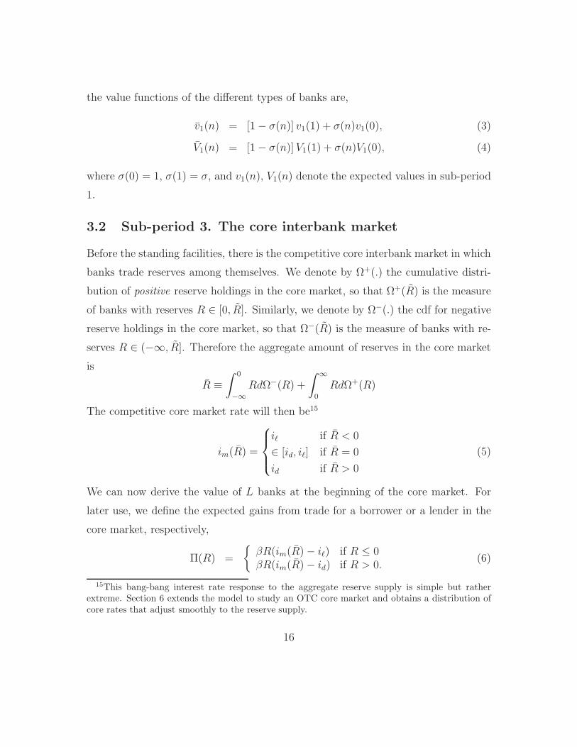
the value functions of the different types of banks are,

v1(n) = [1− σ(n)] v1(1) + σ(n)v1(0), (3)

V1(n) = [1− σ(n)]V1(1) + σ(n)V1(0), (4)

where σ(0) = 1, σ(1) = σ, and v1(n), V1(n) denote the expected values in sub-period

1.

3.2 Sub-period 3. The core interbank market

Before the standing facilities, there is the competitive core interbank market in which

banks trade reserves among themselves. We denote by Ω+(.) the cumulative distri-

bution of positive reserve holdings in the core market, so that Ω+(R) is the measure

of banks with reserves R ∈ [0, R]. Similarly, we denote by Ω−(.) the cdf for negative

reserve holdings in the core market, so that Ω−(R) is the measure of banks with re-

serves R ∈ (−∞, R]. Therefore the aggregate amount of reserves in the core market

is

R ≡ˆ 0

−∞

RdΩ−(R) +

ˆ

∞

0

RdΩ+(R)

The competitive core market rate will then be15

im(R) =

iℓ if R < 0

∈ [id, iℓ] if R = 0

id if R > 0

(5)

We can now derive the value of L banks at the beginning of the core market. For

later use, we define the expected gains from trade for a borrower or a lender in the

core market, respectively,

Π(R) =

βR(im(R)− iℓ) if R ≤ 0βR(im(R)− id) if R > 0.

(6)

15This bang-bang interest rate response to the aggregate reserve supply is simple but ratherextreme. Section 6 extends the model to study an OTC core market and obtains a distribution ofcore rates that adjust smoothly to the reserve supply.

16

Here, a bank with negative balances borrows from the core market at im and avoids

borrowing from the central bank facility at the lending rate iℓ. Similarly, a bank with

R > 0 lends to the core market at im instead of earning the deposit rate id. Then

the value of one L bank with R units of reserves, aggregate dues D, and relationship

status n at the start of the core market is its no-trade payoff augmented with its

expected gains from trade:

V3(R,D, n) = Π(R) + β D +R(1 + i(R))+ βV1(n). (7)

or

V3(R,D, n) = βR(1 + im(R)) + βD + βV1(n).

Obviously V3(R,D, n) is strictly increasing in R with marginal value of reserve β(1+

im(R)).

We now turn to the value of S banks at the start of the core market. The cost γ

of entering the core interbank market may be too prohibitive for some S banks and

hence an S bank only participates in the core market when the gains from trading

Π(R) given by (6) compensate for the entry cost γ. Therefore, the value function of

an S bank at the time of choosing whether to participate or not, given R, is16

v3(R,D, n) = maxΠ(R)− γ, 0+ β D +R(1 + i(R))+ βv1(n). (8)

and using (6) a bank S enters the core market if and only if

βR(im(R)− i(R)) > γ.

So we obtain

16Note that v3 is increasing in R with marginal value β[1 + i(R)] if the bank does not enter themarket, and with marginal value β[1 + im(R)] otherwise.

17

Lemma 1. An S bank enters the core market to borrow iff R ≤ R−and enters to

lend iff R ≥ R+, with Π(R−) = Π(R+) = γ and

R− =−γ

β[iℓ − im(R)], (9)

R+ =γ

β[im(R)− id].

Intuitively, an S bank enters the core market only when it is worth paying the

entry cost. This is the case only if the bank’s reserve balance differs significantly

from the required level 0. Notice that the entry decision does not depend on the S

bank’s relationship status, but only on its reserve holdings. Also, note that the core

interbank rate never falls outside the corridor. We now move on to the (relationship)

trades that occur in the periphery of the core market.

3.3 Sub-period 2. Peripheral trades

In sub-period 2, banks in a pre-established relationship trade their reserves, taking

into account that the core market will open next. Single banks are inactive and their

payoffs are given by (7) and (8) with n = 0. Now consider two banks in a relationship

where the S bank holds RS while the L bank holds RL. We assume that both banks

bargain to determine the loan amount z from the S bank to the L bank as well as the

loan rate i.17 In addition we assume proportional bargaining with weight θ assigned

to S banks.

Obviously, the bargaining outcome depends on the banks’ outside option. If

bank L has been contacted by a single S bank, we assume its threat point with the

incumbent is no trade and breaking up its current relationship. In case of break-

up, the incumbent S bank’s status drops to n = 0, while the L bank gets in a

relationship with the new S bank, and so its status remains n = 1. If bank L has

17We use the convention that bank S lends to banks L whenever z > 0 and borrows from L

whenever z < 0.

18

not been contacted, then the threat point is no trade, but keeping the relationship

into the next period so that n = 1 for both banks.18

From (7) and (8) we can find the trading surplus for an S and an L bank as

a function of the terms of trade, respectively TSS(z, i; c) and TSL(z, i; c), where

c ∈ 0, 1 indicates whether the L bank has been contacted by another S bank

(c = 1) or not (c = 0).19 Then the bargaining problem is

maxz,i

TSS(z, i; c)

subject to

TSL(z, i; c) = (1− θ)[TSS(z, i; c) + TSL(z, i; c)].

We assume that while banks can promise to repay loans the next day, they can

neither commit to trade in the future nor to the terms of trade in future meetings.

For simplicity, we focus on period-by-period bargaining, with the solution given by

the following proposition.20

Proposition 2. (Tiering structure) The size of the relationship loan is RS, the

reserves holdings of the S bank. S banks with a relationship never enter the core

market.

This result is intuitive. As derived in the Appendix, the loan size z is chosen

to maximize the total surplus, given the banks’s reserves, while the rate i is chosen

to split the surplus according to the surplus-sharing protocol. Since bank L can

access the core market at no cost, it will provide intermediation by absorbing all the

(excess) reserves of bank S (positive or negative) while bank S can avoid the entry

18These threat points are subgame-perfect.19The details are in the Appendix.20Given reserves holdings, the terms of trades under full or limited commitment are the same.

However, reserve holdings can differ with the degree of commitment for a simple reason: In theabsence of commitment, banks internalize the fact that they can be cornered by their tradingpartner, which induces them to adopt a suboptimal bidding strategy at the central bank tender.

19

cost.21 The relationship rate is the price bank S pays to bank L to intermediate the

access to the core market. Using the solution to the bargaining problem above, it

is easy to see that the relationship rate splits the gains from trade according to the

bargaining power. The gains from trade are made of three components: First, bank

S’ opportunity cost of using bank L as an intermediary, i.e.

maxβ[1 + i(RS)]RS,−γ + β[1 + im(R)]RS.

Second, bank L’s benefit of intermediating bank S’ balances

[1 + im(R)]RS.

Third, bank S’s willingness to pay to retain the relationship with bank L, whenever

it is contacted by another bank, i.e.

(1− σ)v1(1) + σv1(0)− v1(0)

Defining

V ≡ −(1 − σ)[v1(1)− v1(0)]

as the cost for bank S of giving up the relationship, we can then write the relationship

rate from the bargaining problem as

1 + i(RS, RL, c) = (1− θ)maxβ[1 + i(RS)]RS,−γ + β[1 + im(R)]RS

βRS

(10)

+θ[1 + im(R)] + (1− θ)cVRS

,

where c = 1 if bank L was contacted, and c = 0 otherwise. Using (6) and the entry

decision of single banks we obtain

i(RS, RL, c) =

θim(R) + (1− θ)i(RS) + (1− θ) cVRS

, if no entry when single

θim(R) + (1− θ)[

im(R)− γ

βRS

]

+ (1− θ) cVRS

, if entry when single

(11)

21The centralized structure of the core market guarantees that the L bank can always trade.Hence, there is no need for S banks in a relationship to enter the core market. When the coremarket is OTC instead of centralized, S banks in a relationship may still enter the market to insureagainst the event that the L bank would not find a proper match.

20

Notice that the relationship rate is only a function of RS, and that the rate with no

entry is always smaller than the rate with entry. The relationship rate is a sum of two

parts. The first part is a weighted sum of the L bank’s benefit of obtaining RS and

the S bank’s opportunity cost of giving up RS. This part is always between id and

iℓ. The second part V/RS is the S bank’s cost of giving up the relationship. This

part can be positive or negative depending on whether the S bank is a borrower

or a lender. Comparing the relationship rate and the core rate, we can define a

relationship premium as follows.

Lemma 3. The relationship rate is i(RS, c) = im(R) − P (RS) where P (RS) is the

relationship premium defined as,

P (RS) = (1− θ)

[

minim(R)− i(RS),γ

βRS

− cVRS

]

,

with P (RS) > 0 for RS > 0 and P (RS) < 0 for RS < 0.

The relationship premium captures how much relationship rates i of peripheral

trades deviate from the core rate im. When S banks do not have full bargaining

power (i.e. θ < 1), the premium is non-zero when the S banks value the relationship

(i.e. V=-(1-σ)[v1(1)− v1(0)] <0) and the L bank can immediately rebuild a new one

(i.e. c = 1). Also, the premium is non-zero when it is costly to enter the core market

(i.e. γ > 0). Notice that whenever the S bank is a lender (RS > 0), V/RS is negative

as long as the S bank values the relationship. In this case, the relationship rate is

driven down. Similarly, whenever the S bank is a borrower (RS < 0) the relationship

rate is raised as the S bank values the relationship.22 In addition, when V= 0, the

relationship rate always stays within the corridor. Otherwise, the relationship rate

can fall below id or go above iℓ. We formalize this result in the following corollary,

22Interestingly, this is consistent with the finding by Ashcraft and Duffie (2007) that “[t]he ratenegotiated is higher for lenders who are more active in the federal funds market relative to theborrower. Likewise, if the borrower is more active in the market than the lender, the rate negotiatedis lower, other things equal.”

21

Corollary 1. Relationship rates for peripheral trades may fall outside of the corridor

when the L bank is contacted by an S bank: With RS > 0, i(RS) < id iff

im(R) < id −(1− θ)VθRS

.

With RS < 0, i(RS) > iℓ iff

im(R) > iℓ −(1− θ)VθRS

.

This concludes the analysis of trades between two banks in a relationship. To

summarize, S banks use the L bank as an intermediary to access the interbank

market and may even agree to pay a premium to continue the relationship. So the

relationship rate could well hover above iℓ whenever the S bank is borrowing from

the L bank, or below id whenever it is lending to L.

3.4 Sub-period 2. Relationship-building calls

Before peripheral trades, single S banks can pay a cost κ to contact a bank L. At

this stage, all single S banks are the same, so either they all pay the cost, or none of

them do, or they use a mixed strategy if they are indifferent.

To be precise, at the start of sub-period 2, a fraction 1 − NL of L banks are

in a relationship and a fraction NL is single. Therefore, a single S bank searching

contacts a single L with probability NL. Also an L bank expects a contact with

probability NS, where NS is the fraction of S banks that are single and searching.

The fraction of L (and S) banks in a relationship is 1−NL. So at the beginning

of sub-period 2 the fraction of L banks that are single are all but (a) those who were

in a relationship last period and the relationship was not severed, and (b) those who

were not in a relationship last period, got a contact and the new relationship was

not severed:

NL = 1− [(1−NL)(1− σ)︸ ︷︷ ︸

(a)

+NLNS(1− σ)︸ ︷︷ ︸

(b)

],

22

or

NL =σ

(1− σ)NS + σ. (12)

S banks search whenever the expected benefit is higher than the search cost κ. Hence,

the fraction of S banks searching is

NS =

NL if NL(1− σ)β[v1(1)− v1(0)] > κ

0 if NL(1− σ)β [v1(1)− v1(0)] < κ

[0, NL] otherwise

(13)

The left-hand side of the above inequality condition captures that a single S bank

successfully finds a single L bank with probability NL, in which case a new relation-

ship is formed but only survived with probability 1 − σ, in which case it brings a

surplus v1(1)− v1(0) from the next period onward.

3.5 Sub-period 1. Central bank tender

We now define the expected payoffs of different types of banks at the end of subperiod

1. We use mn and Mn to denote, respectively, the reserve balances of S and L banks

with relationship status n ∈ 0, 1 when they exit the central bank tender but before

they know their liquidity shock. Define M = (M0,M1, m0, m1) and let the dues from

the relationship loan be D(RS, c), where again c = 1 if bank L has been contacted

by another S bank, and c = 0 otherwise, i.e. D(RS, c) = [1 + i(RS, c)]RS. Then the

expected value of a matched L bank with reserve holdings M before the shock is

V2(M, 1;M) =

ˆ

∞

−∞

ˆ

∞

−∞

Ec [V3(M + ε+m1 + ξ,−D(m1 + ξ, c), 1)]dG(ε)dF (ξ)+βV1(1)

and in the Appendix, we show that bank L’s marginal benefit of an extra dollar is

just the discounted benefit of lending this extra dollar in the core market, i.e.

∂V2(M, 1;M)

∂M= β(1 + im(R)). (14)

23

Similarly, the expected value of a bank S in a relationship holding reserves m1 before

the shock is

v2(m1, 1;M) =

ˆ

∞

−∞

Ec [v3(0, D(m1 + ξ, c), 1)] dF (ξ) + βv1(1)

When choosing m1, the S bank takes into account how it affects the probability of

accessing the core market. In the Appendix, we show that the value of the marginal

dollar is

∂v2(m1, 1;M)

∂m1

= β(1 + im(R)

)+ β(1− θ)

[id − im(R)

] [

F(

R+ −m1

)

− F (−m1)]

+β(1− θ)[iℓ − im(R)

] [

F (−m1)− F(

R− −m1

)]

(15)

where R+ and R− are given by (9). The first term is the discounted benefit of lending

this extra dollar in the core market when the S bank enters the core market. The

second and third terms capture the additional values when the S bank passes the

core market to use the central bank facilities. Notice that if im(R) = (iℓ+ id)/2 then

∂v2(m1, 1;M)/∂m1 = β(1 + im(R)

).

The expected value of a single L bank holding M units of reserves before the

shock is V2(M, 0;M) defined in a similar way as above, and the value of an extra

dollar for a single L bank is also the discounted value of lending this extra dollar in

the core market:∂V2(M, 0;M)

∂M= β(1 + im(R)). (16)

Finally, the expected value of a single S bank holding reserves m before the shock,

is v2(m0, 0;M) defined as above, and the value of an extra dollar for this bank is

∂v2(m0, 0;M)

∂m0

= β(1 + im(R)

)+ β

[id − im(R)

] [

F(

R+ −m0

)

− F (−m0)]

+β[iℓ − im(R)

] [

F (−m0)− F(

R− −m0

)]

. (17)

Notice that relative to (15), the single S bank fully internalizes the benefit/cost of

this extra dollar, as it does not have to share it with an L bank.

24

In sub-period 1, the central bank offers to sell and buy reserves at a rate i.23 This

“tender” consists of one-period loans of reserve balances, which will be paid back in

the next settlement stage. Expecting that other banks will bid M, the decision of

an L bank with n ∈ 0, 1 is:

V1(n) = maxMn

−β(1 + i)Mn + V2(Mn, n;M)

and

v1(n) = maxmn

−β(1 + i)mn + v2(mn, n;M).

The first-order conditions for L banks are

∂V2(Mn, n;M)

∂Mn

= β(1 + i), (18)

and similarly for S banks,

∂v2(mn, n;M)

∂mn

= β(1 + i). (19)

So, we can find the bids of each bank using (14)-(17). In equilibrium the choice

of reserves of individual banks should be consistent with M. Also, notice that if

i > iℓ, then banks can earn infinite risk-free profit by holding an infinitely large

negative amount of reserves; if i < id, then banks can earn infinite risk-free profit

by holding an infinitely large positive amount of reserves. Therefore, no arbitrage

requires i ∈ [id, iℓ].

Given M, the excess reserves in the core market R are given by

R =1−NL

2M0 +

NL

2M1 +

1−NL

2

ˆ

(m0 + ξ)Ie(m0 + ξ)dF (ξ) +NL

2m1

where Ie = 1 when a bank S enters the core market and Ie = 0 when it does not. Since

L banks always enter the interbank market, there are 1−NL single L banks holding

23An alternative view, which is more in line with some central banks’ practice, is that the centralbank supplies/purchases M units of reserves and banks bid a schedule of rates and correspondingreserves amount they are willing to obtain at this rate. Market clearing implies

∑

n Mn+mn = M ,and the stop-out rate is i, such that the first-order condition of each bank holds.

25

M0. But only those 1−NL single S banks that sustained a large enough shock ξ will

pay the entry cost. Finally, as L banks in a relationship always intermediate entry in

the centralized interbank market for S banks, the average L bank in a relationship

enters the relationship market with M1 +m1. From (5) and the above conditions, it

is straightforward to show that

Proposition 4. im(R) = i and we only have three types of equilibrium (and policy

rate):

i =

iℓ , mn = −∞ and Mn such that R < 0iℓ+id

2, mn = 0 and Mn such that R = 0

id , mn = ∞ and Mn such that R > 0

Also, NS > 0 (i.e. S banks search) only if i = (iℓ + id)/2.

This means that only the policy rate set at the midpoint of the corridor will induce

relationship formation. This is due to the centralized structure of the core market.

As we show in our companion paper, it is possible to eliminate the extreme cases

by extending the model to have a core market with an OTC instead of a centralized

structure.

4 Characterization of the equilibrium

We can now define an equilibrium. Recall that M = Mn, mnn=0,1. Then,

Definition 5. Given i ∈ id, iℓ+id2

, iℓ a steady-state equilibrium is a list NS, NL,Mconsisting of the fraction NS of single S banks searching, the fraction NL of single L

banks, and the banks’ money demand M, such that, given the policy rates i, id, and

iℓ, the search decision by S banks, reserves holdings, and entry by S banks in the

core market are optimal and consistent with the bargaining solutions.

Let

Γ ≡ˆ

∞

−∞

βθ

[

Ieγ

β+ Ine

[iℓ + id

2− i(ξ)

]

ξ

]

dF (ξ)

26

be the expected per-period benefit of a relationship for the S bank when the rate

in the centralized market is at the midpoint of the corridor. Then we obtain the

existence and uniqueness of the equilibrium.

Proposition 6. A unique equilibrium exists. When i ∈ id, iℓ then NS = 0 and

there is no relationship. When i = (iℓ + id)/2 then there are three cases, with

κ =β(1− σ)

[1− β(1− σ)]Γ, and κ =

N∗

L(1− σ)β

[1− β(1− σ) (1−N∗

L(1− θ))]Γ,

(1) When κ < κ, all single S banks search, NS = N∗

L =−σ+

√σ2+4(1−σ)σ

2(1−σ), and

v1(1)− v1(0) =Γ + κ

1− β(1− σ) (1−N∗

L −N∗

S(1− θ)).

(2) When κ ∈ [κ, κ], S banks use a mixed strategy and NS = NS given by (C.1),

and

v1(1)− v1(0) =Γ

1− β(1− σ)[1− NS(1− θ)

] .

(3) When κ > κ, S banks do not search, NS = 0, and

v1(1)− v1(0) =Γ

1− β(1− σ).

Proof. We relegate the proof to the Appendix.

Intuitively, when κ is low, all single S banks will try to build a relationship.

When κ is high, there is no relationship lending because it is too costly for S banks

to build one. For the intermediate level of κ, single S banks are indifferent between

building a relationship and staying single.

5 Qualitative implications

This section derives some qualitative implications of the benchmark model. Specifi-

cally, we study (i) how policy and other parameters affect the network structure of

27

the interbank market, (ii) why interbank rates can go below the floor in the short

run and in the long run, (iii) how the interbank market will react dynamically to an

exit from a floor system, and (iv) how regulation on exposure limits can affect the

interbank market.

5.1 Interbank network

To study the network structure of interbank trades, we first derive some comparative

statics on the entry decision of single banks in the core market. Recall that the entry

decision by single S banks is given by the two thresholds defined in (9). Since

im ∈ id, (iℓ + id)/2, iℓ, these thresholds only depend on the corridor size iℓ − id. As

a consequence the relationship benefits Γ also depend on the corridor size iℓ − id.

Lemma 7. When i = (iℓ + id)/2, the per-period gains from a relationship Γ is

increasing in iℓ − id, θ, and the variance of the shock ξ. Also Γ → 0 when iℓ → id.

As a relationship provides intermediation to the core market, the expected benefit

of a relationship for the S banks increases when the corridor is wider, their bargaining

power is higher and the liquidity shock is more uncertain.24 As a consequence, S

banks’ incentives to search and build relationships are affected by the same set of

variables.

Lemma 8. κ,κ and NS are increasing in iℓ − id, θ, and the variance of the shock ξ,

and NS is decreasing in κ. NS → 0 as iℓ → id.

In words, single S banks search more actively when the gains from relationship

lending are larger (that is, when the corridor is larger), when they have more bar-

gaining power, or when the variance of the shock is higher. Naturally, they search

less when the cost of searching is higher. Finally, single S banks do not search if

iℓ = id, as in this case there is no gain from trade.

24If 2 >f(x)x1−F (x) for all x > 0 then Γ is also increasing in γ.

28

After examining the trades among banks, we now study the usage of standing

facilities and derive the amount borrowed from or deposited at the standing facility.

Access to the two standing facilities is determined by the amount of excess reserves

in the centralized market R together with the usage of the facilities by single S banks

that do not enter the core market. So, access to the lending facility when the policy

rate is at the midpoint of the corridor (i.e. R = 0) is

1

2

σ

(1− σ)NS + σ

ˆ

−m0

R−

(m0 + ξ)dF (ξ) =1

2

σ

(1− σ)NS + σ

ˆ 0

R−

ξdF (ξ)

The integrand is decreasing as iℓ−id increases, andNS is either constant or increasing:

As it is more costly to stay out of the core market, single banks tend to search more

and enter the core market more frequently. As a result, there is a lower access to the

lending facility (and also for the deposit facility).25

Finally, we study how the corridor width affects the network size. Recall that

Beltran, Bolotny, and Klee (2015) show a decline in the number of loans from pe-

ripheral banks to core banks as the Fed reduced the corridor size. Hence, we should

expect a positive relationship between the width of the corridor and the number of

relationship loans. In our model, the size of the peripheral network P is defined by

the measure of banks in a relationship. This is 1−NL, or

P = 1− σ

(1− σ)NS + σ

which is positively correlated with NS. Hence, as the corridor increases, more S

banks search and the size of the peripheral network P increases, as in the data.

The size of the core network C is defined by 1/2 measure of L banks as well as

25Access to the deposit facility is

1

2

σ

(1− σ)NS + σ

ˆ R+

−m0

(m0 + ξ)dF (ξ).

29

single S banks that enter the core market, or

C =1

2+

1

2NL

[

1− F (R+) + F (R−)]

=1

2+

1

2

σ

(1− σ)NS + σ

[

1− F (R+) + F (R−)]

.

As the corridor increases, there are two counteracting effects: (1) more S banks are

in a relationship, which decreases C, but (2) those S banks with no relationship enter

the core market more often, thus increasing C. So the effect of an increasing corridor

on the size of the network in the core market C is indeterminate, but the volume of

trade in the core market will increase. Finally, single and inactive S banks always

access the standing facilities and there is a fraction I of such banks,

I =1

2

σ

(1− σ)NS + σ

[

F (R+)− F (R−)]

.

As for C, the effect of an increase in the corridor on I is indeterminate.

Finally, we used the labels L and S as standing for large and small. Even when

F = G and there is no difference between these two banks ex ante, aside from their

access to the core market, L and S banks will tend to look large and small in equi-

librium. Indeed, when they are matched, S banks will always use the intermediation

provided by the L bank to indirectly access the core market. As a result, the L bank

will trade more often and larger amounts than S banks.

5.2 Trades below the floor

As discussed in the introduction, at times, banks have been trading outside of the

corridor, even though they had access to the central bank standing facilities at no

cost, especially when there is excess liquidity in the banking system. How can our

model match this fact? We will provide conditions under which the interbank rate

may fall below the floor of the corridor id both in the steady state and in response

to a temporary liquidity shock.

30

(i) Steady state

Below, we show that S banks with a relatively small ξ > 0 will trade below the

floor whenever their L bank partner has been contacted by a single S bank. We

already showed that when NS > 0, the relationship loans rate may fall outside of the

corridor, i.e. i(RS) < id if and only if m1 + ξ > 0 and

im(R) < id −(1− θ)Vθ(m1 + ξ)

,

or i(RS) > iℓ if and only if m1 + ξ < 0 and

im(R) > iℓ −(1− θ)Vθ(m1 + ξ)

.

Recall that there are no relationships except when the policy rate is at the midpoint

of the corridor. In that case m1 = 0 and im(R) = (iℓ + id)/2. Then the relationship

rate falls below the floor whenever bank S is holding ξ > 0 relatively small, or26

(iℓ − id)

2ξ <

(1− θ)

θ(1− σ)[v1(1)− v1(0)],

where v1(1) − v1(0) is given in Proposition 6. As iℓ → id, we have R+ → ∞ and

R− → −∞, as well as

Γ → βθ

[iℓ − id

2

]

2

ˆ

∞

0

ξdF (ξ).

While NS → 0, all S banks in a relationship receiving shock ξ such that

ξ <2(1− θ)β(1− σ)

´

∞

0ξdF (ξ)

1− β(1− σ),

26When NS = NS , this expression becomes

ξ <(1− θ)

θ

(1 − σ)Γ(iℓ−id

2

) [1− β(1− σ)

[1− NS(1− θ)

]] ,

while when NS = N∗

L =−σ+

√σ2+4(1−σ)σ

2(1−σ) it is

ξ <(1− θ)(1 − σ)

θ(iℓ−id

2

)Γ + κ

[1− β(1− σ) (1−N∗

L(2− θ))].

31

will trade below the floor. That is, with a small corridor, while there are fewer

relationships, it is more likely for a relationship trade to occur below the floor.

(ii) Temporary liquidity shock

We now consider a temporary liquidity shock to the interbank market. Consider a

steady-state equilibrium in which the central bank sets i = (iℓ+ id)/2 and thus there

are banks in active relationships. Suppose the central bank mistakenly allocates extra

reserves so that there is a (small) amount of excess reserves in the core market, R > 0,

only for the current period.27 Hence, the interbank rate falls to the floor im(R) = id.

In addition, the central bank’s mistake does not affect the search behavior of S banks

and thus V remains at its steady-state value, which is negative. From (11), we have

i(RS, c) =

id +c(1−θ)V

RS, if no entry when single,

id − (1− θ) γ

βRS+ c(1−θ)V

RS, if entry when single.

As a result, all relationship loans from an S bank to an L bank (i..e. RS > 0) that

has a contact (i.e. c = 1) are traded below the floor.

5.3 Exit from a floor system

In response to the recent financial crisis, many central banks have moved their mon-

etary implementation framework from a symmetric corridor system to a floor system

by significantly increasing reserve balances and setting the target rate at the bottom

instead of the midpoint of the corridor. One natural question is how the interbank

market will react when the central bank decides to exit from the floor system and

return to the conventional corridor system. To answer this question, we derive the

transition path as the interbank market converges from the old to the new steady-

state equilibrium.

27An alternative interpretation is that the central bank conducts a short-term intervention byinjecting liquidity into the market with a commitment to withdraw it in the next period. SeeBerentsen and Waller (2011).

32

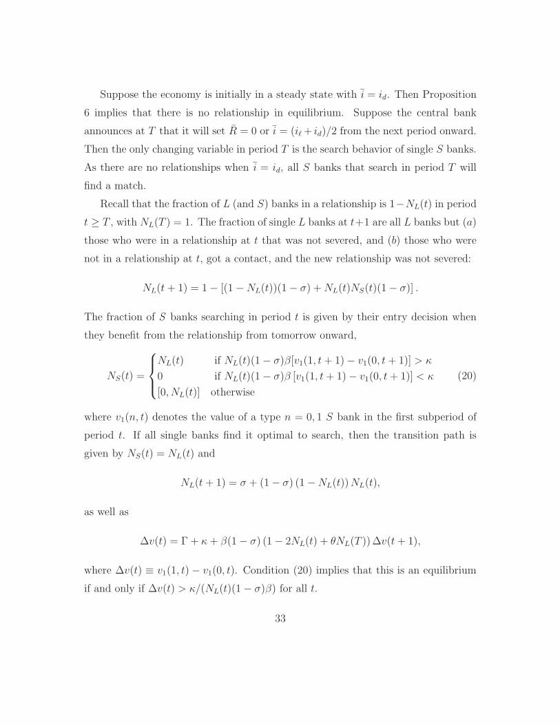
Suppose the economy is initially in a steady state with i = id. Then Proposition

6 implies that there is no relationship in equilibrium. Suppose the central bank

announces at T that it will set R = 0 or i = (iℓ+ id)/2 from the next period onward.

Then the only changing variable in period T is the search behavior of single S banks.

As there are no relationships when i = id, all S banks that search in period T will

find a match.

Recall that the fraction of L (and S) banks in a relationship is 1−NL(t) in period

t ≥ T , with NL(T ) = 1. The fraction of single L banks at t+1 are all L banks but (a)

those who were in a relationship at t that was not severed, and (b) those who were

not in a relationship at t, got a contact, and the new relationship was not severed:

NL(t + 1) = 1− [(1−NL(t))(1− σ) +NL(t)NS(t)(1− σ)] .

The fraction of S banks searching in period t is given by their entry decision when

they benefit from the relationship from tomorrow onward,

NS(t) =

NL(t) if NL(t)(1− σ)β[v1(1, t+ 1)− v1(0, t+ 1)] > κ

0 if NL(t)(1− σ)β [v1(1, t+ 1)− v1(0, t+ 1)] < κ

[0, NL(t)] otherwise

(20)

where v1(n, t) denotes the value of a type n = 0, 1 S bank in the first subperiod of

period t. If all single banks find it optimal to search, then the transition path is

given by NS(t) = NL(t) and

NL(t + 1) = σ + (1− σ) (1−NL(t))NL(t),

as well as

∆v(t) = Γ + κ+ β(1− σ) (1− 2NL(t) + θNL(T ))∆v(t+ 1),

where ∆v(t) ≡ v1(1, t)− v1(0, t). Condition (20) implies that this is an equilibrium

if and only if ∆v(t) > κ/(NL(t)(1− σ)β) for all t.

33

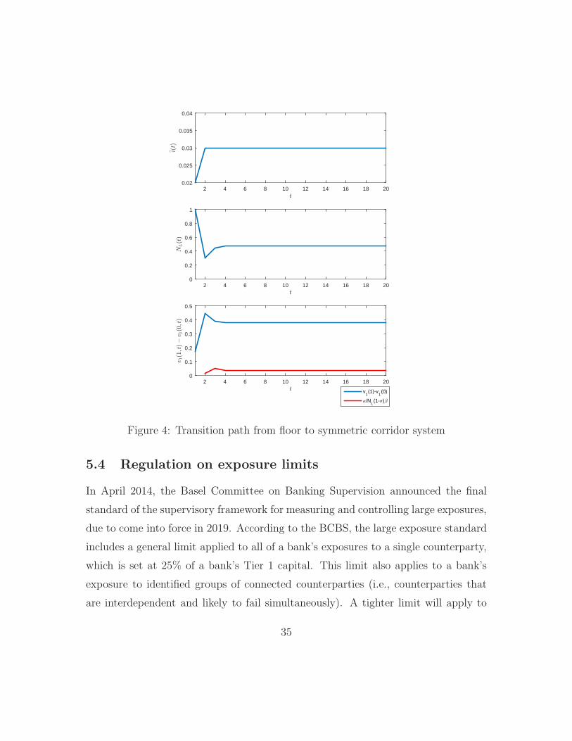
As t → ∞ the economy converges to the steady state where all single banks

search. However, the convergence is not necessarily monotonic, as shown in Figure

428: When the central bank announces the start of the exit policy, all S banks search if

the value of a relationship to a single S bank becomes sufficiently positive, and above

κ/(NL(t)(1 − σ)β). When all banks search, many are successful, as all L banks are

single. So the number of relationships is maximized at T + 1 (i.e., NL is minimized)

and N(T+1) is relatively small. The value of having a relationship is also maximized:

As few S banks will be unmatched at T , it becomes less likely for matched L banks

to be contacted in the following periods. Similarly, as many L banks are already in a

relationship, it is also harder for a single bank to build a new relationship. Following

this undershoot, NL(t) creeps back up and gradually converges (with or without

oscillations) to its new steady-state value. In the Appendix we derive the transition

path for the case when single banks are indifferent between searching and not.

28In the figure, we set T = 0.

34

2 4 6 8 10 12 14 16 18 20

0.02

0.025

0.03

0.035

0.04

2 4 6 8 10 12 14 16 18 20

0

0.2

0.4

0.6

0.8

1

2 4 6 8 10 12 14 16 18 20

0

0.1

0.2

0.3

0.4

0.5

v1(1)-v

1(0)

/NL(1-)

Figure 4: Transition path from floor to symmetric corridor system

5.4 Regulation on exposure limits

In April 2014, the Basel Committee on Banking Supervision announced the final

standard of the supervisory framework for measuring and controlling large exposures,

due to come into force in 2019. According to the BCBS, the large exposure standard

includes a general limit applied to all of a bank’s exposures to a single counterparty,

which is set at 25% of a bank’s Tier 1 capital. This limit also applies to a bank’s

exposure to identified groups of connected counterparties (i.e., counterparties that

are interdependent and likely to fail simultaneously). A tighter limit will apply to

35

exposures between banks that have been designated as global systemically important

banks (G-SIBs). This limit has been set at 15% of Tier 1 capital. While there is no

counterparty risk in our model, we can still analyze the effect of the regulation on

the functioning of the interbank market and its network. To do so, we assume that

banks in a relationship can only lend up to a limit B > 0, equivalent to x% of their

Tier 1 capital.

Since the core market is a centralized market, banks can borrow from many

counterparties bearing limited exposure to each of them. Therefore in our simple

model, the constraint will not bind in the core market. However, it may bind in the

peripheral market. When the exposure limit does not bind, banks trade RS and, as

before, bank S does not enter the core market. However, if the exposure limit binds,

banks trade B and bank S still holds RS − B if RS > 0 and RS +B when RS < 0.

In other words, the size of the loan from the S to the L bank is z(RS , RL) = B if

RS > 0 and z(RS , RL) = −B otherwise. Then, S banks will enter the core market

whenever they still hold too much or too few reserves,

Lemma 2. An S bank enters the core market to borrow RS + B iff RS + B ≤ R−

and enters to lend RS −B iff RS −B ≥ R+, where R− and R+ are defined in Lemma

1.

Then banks decide on the rate i so that bank L takes a share θ of the total surplus

so that the rate for the relationship loan is given by,

1 + i(RS, RL;B) = (1− θ)v3(RS, 0, 0)− v3(RS − z(RS , RL), 0, 0)

βz(RS, RL)(21)

+ θV3(RL + z(RS , RL), 0, 0)− V3(RL, 0, 0)

βz(RS, RL)+

cVz(RS , RL)

,

and using the expressions for v3 and V3, and noticing that i(RS) = i(RS − z) when

36

the exposure limit binds, we obtain

1 + i(RS, RL;B) = (1− θ)maxΠ(RS)− γ, 0 −maxΠ(RS − z(RS))− γ, 0

βz(RS)(22)

+ (1− θ)(1 + i(RS)) + θ(1 + im(R)) +cV

z(RS).

Notice that as B → ∞, z(RS) → RS so that maxΠ(RS − z(RS)) − γ, 0 → 0.

Hence, the relationship rate is lower when bank S is lending (z(RS) > 0) and higher

otherwise, as gains from trade are smaller. As a consequence, the value of the

relationship is lower and we should expect to have a lower number of relationships

in equilibrium. Hence, the regulation on bilateral exposure will distort relationship

formation and change the interbank network structure.

6 Quantitative implications of the OTC interbank

market

Our assumption that banks trade in a centralized market has three important con-

sequences. First any amount of excess reserves drives the interbank rate to the floor

id of the corridor, while any amount of reserves deficit drives the interbank rate to

its ceiling iℓ. There is only a middle ground when there are no excess reserves (or

deficit); then the interbank rate is the midpoint of the corridor. Second, S banks

adopt extreme bidding strategies except when the policy rate is in the midpoint of

the corridor, in which case they bid zero reserves. Finally, S banks in a relationship

never find it optimal to access the core market. These three results are at odds with

the data.

We now relax the assumption that the core market is frictionless and instead

assume it is over-the-counter (OTC). Below, we summarize the main findings, while

detailed analysis and proofs can be found in our companion paper. In this OTC

core market, banks can meet pairwise according to a simple matching function, as

in Bech and Monnet (2014): a bank (S or L) that wants to borrow reserves can only

37

meet a bank (S or L) with a desire to lend reserves. Then the two banks negotiate

over the terms of trade (x, r) where x denotes the loan size and r denotes the loan

rate. Although they could, we retain the assumption that banks cannot create a

relationship in this market. The rest of the economy is as described above.

Unsurprisingly, we cannot obtain closed-form solutions in the case with an OTC

market. However, we show that, as in Bech and Monnet, (1) the OTC rate is now

a weighted average of the rates that are bilaterally negotiated, so that it can be

strictly within the corridor even though there is an excess or a deficit of reserves. (2)

The OTC rate can never lie outside of the corridor, and only the relationship rates

can. (3) Banks do not bid an extreme amount of reserves. Finally (4) S banks in a

relationship may sometimes find it optimal to enter the core market even though it

is costly. Precisely,

Proposition 9. Let the core market be OTC. Consider a pair of banks in a rela-

tionship holding balances RS and RL in the periheral market. There are reserves

thresholds R− < 0 and R+ > 0 such that if RS +RL ∈ [R−, R+] then the S bank does

not enter the core market. Otherwise the S bank enters the core OTC market. The

size of the relationship loan is

z(RS , RL) =

RS if RS +RL ∈ [R−, R+]

(RS − RL) /2 otherwise.

The reason is simple: As the core market is now frictional, sometimes L bank

cannot find any other bank to trade or can only find a bank that is not such a

good match. This is particularly costly when the L bank is carrying a large reserve

surplus or deficit. To insure against such bad luck, the S bank may find it optimal

to “share the burden” and pay the fixed entry cost to the core market. This will be

so when the S and L banks hold a large reserve surplus or deficit.29 Naturally, rates

29In this case, it may be that the L bank lends to the S bank before the S bank enters the coremarket.

38

for relationship trades may still fall outside of the corridor for the same reasons as

before, although the formulation for the rate is now more complicated.

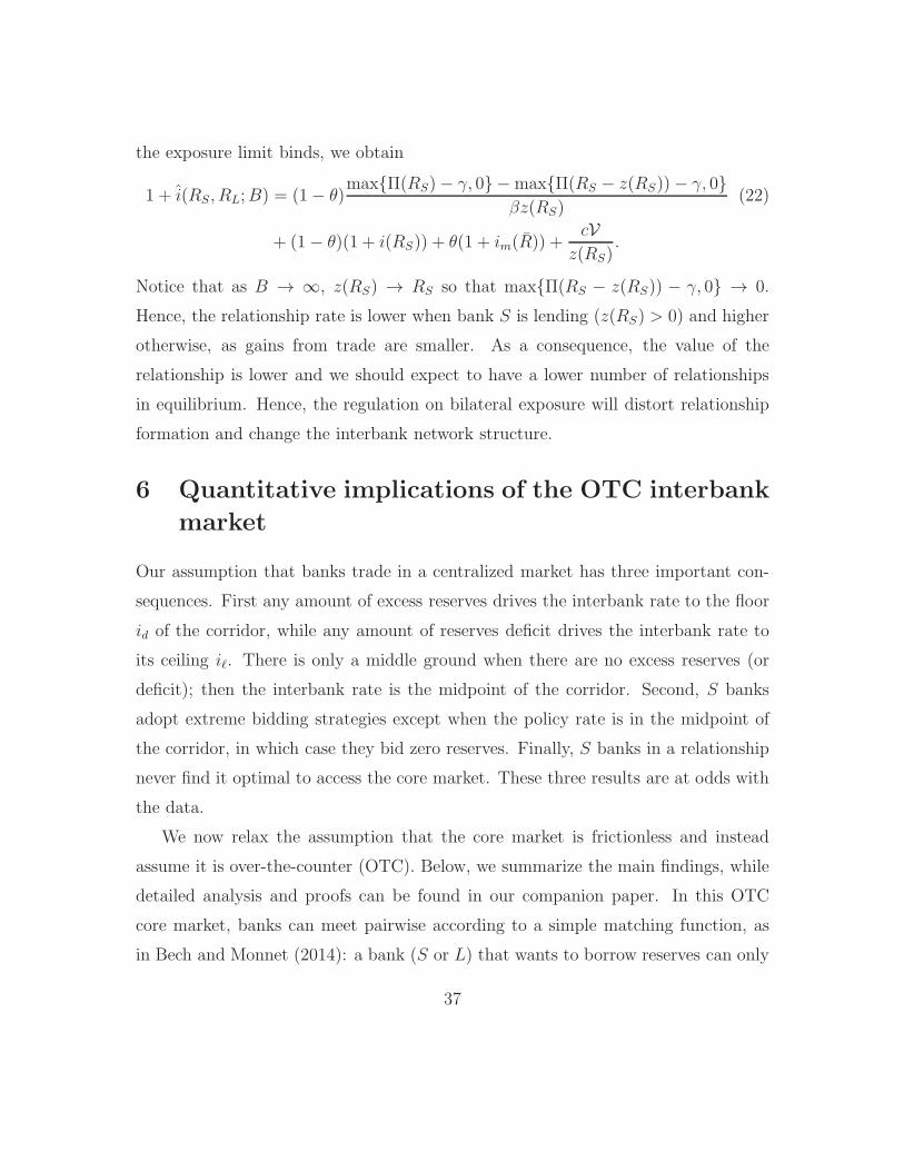
In the sequel, we report the following statistics for a parameterized model with

an OTC core market: The values of relationship loans, OTC loans, deposits with the

central bank by S and L banks, total borrowing at the lending facility by S and L

banks, single and matched. We present the details in the companion paper.

6.1 Parameterization

The discount factor for banks is β = 0.97. Liquidity shocks ε for L banks are

drawn from a normal distribution N (−1, 2), while liquidity shocks ξ for S banks are

drawn from a distribution N (1, 2). Therefore, S banks tend to have liquidity inflows

(i.e., potential liquidity providers) and L banks tend to have liquidity outflows (i.e.,

potential liquidity demanders), even though in aggregate there are no net inflows

or outflows. This is consistent with the observations that small banks tend to be

liquidity providers to large banks (Stigum and Crescenzi, 2007).

In sub-period 2, the cost for S banks to search and build a new relationship is

κ = 0.0001, and the probability of separation is σ = 0.1. In the OTC market, the

number of matches is given by

min(N+)0.5(N−)0.5, N+, N−.

where N+ is the total measure of banks (S or L) with excess reserves, while N− is

the total measure of banks with a reserve deficit. The cost for S banks to search

in this market is γ = 0.0005. Borrowers and lenders have equal bargaining powers:

θ = Θ = 0.5 in both peripheral and core trades. The lending and deposit rates are

given by id = 2% and iℓ = 4%. In the following, we will examine the effect of applying

different policy rates i. While the parameter values are ad hoc, the implication of

the model is qualitatively robust to parameter changes. The numerical algorithm for

solving the steady-state equilibrium is described in the Appendix.

39

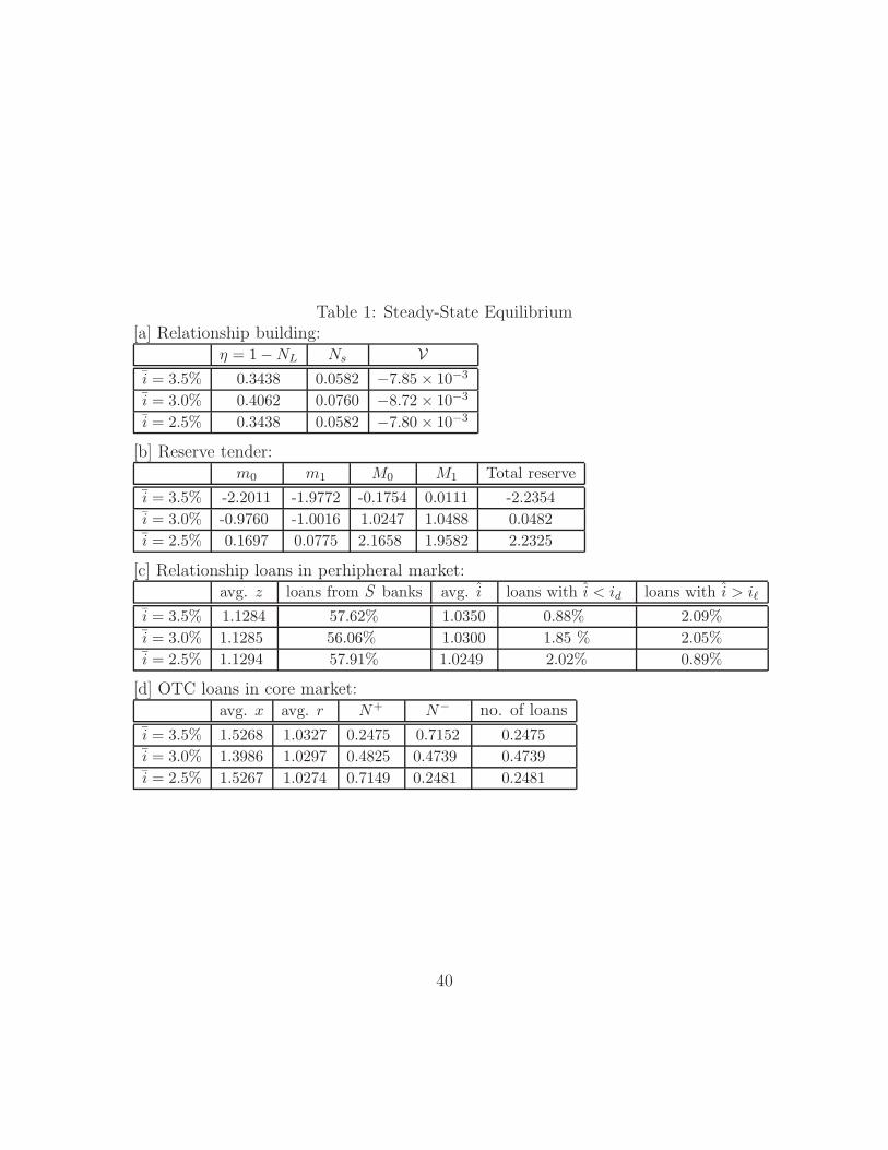
Table 1: Steady-State Equilibrium[a] Relationship building:

η = 1−NL Ns Vi = 3.5% 0.3438 0.0582 −7.85 × 10−3

i = 3.0% 0.4062 0.0760 −8.72 × 10−3

i = 2.5% 0.3438 0.0582 −7.80 × 10−3

[b] Reserve tender:m0 m1 M0 M1 Total reserve

i = 3.5% -2.2011 -1.9772 -0.1754 0.0111 -2.2354

i = 3.0% -0.9760 -1.0016 1.0247 1.0488 0.0482

i = 2.5% 0.1697 0.0775 2.1658 1.9582 2.2325

[c] Relationship loans in perhipheral market:avg. z loans from S banks avg. i loans with i < id loans with i > iℓ

i = 3.5% 1.1284 57.62% 1.0350 0.88% 2.09%

i = 3.0% 1.1285 56.06% 1.0300 1.85 % 2.05%

i = 2.5% 1.1294 57.91% 1.0249 2.02% 0.89%

[d] OTC loans in core market:avg. x avg. r N+ N− no. of loans

i = 3.5% 1.5268 1.0327 0.2475 0.7152 0.2475

i = 3.0% 1.3986 1.0297 0.4825 0.4739 0.4739

i = 2.5% 1.5267 1.0274 0.7149 0.2481 0.2481

40

6.2 Effects of policy on rates and volumes

Table 1 and Figure 5 report equilibrium outcomes under different policy rates. We

first consider the equilibrium outcome under a symmetric corridor system with i =

0.5(id + iℓ) = 3%. Banks’ reserve demand at the tender is reported in table 1b and

also plotted in the top left panel of Figure 5. Note that, unlike the benchmark model,

this model implies a reserve demand that responds smoothly to changes in the policy

rate. As expected, due to their different shock distribution, S banks bid less reserves

than L banks. In particular, anticipating a liquidity shock with mean E(ξ) = 1, S

banks tend to hold a negative reserve position close to−1, while L banks, anticipating

a liquidity shock with mean E(ε) = −1, tend to hold a positive reserve position close

to 1. Since there is no aggregate liquidity shock, the total reserve demand is close

to zero (i.e., the minimum reserve requirement) under a symmetric corridor system.

The total reserve demand is similar to that in the benchmark model when the policy

rate is set at the midpoint of the corridor.

As the policy rate gets closer to the deposit rate, banks find it cheaper to hold

more reserve balances to self insure against the risk of accessing the lending facility.

As a result, the total demand for reserves increases, and all banks choose a positive

initial reserve position. Symmetrically, as the policy rate gets closer to the lending

rate, banks prefer to try financing their liquidity needs in the markets, and the total

demand for reserves at the tender declines so that most banks choose a negative

initial reserve position.

Banks’ initial demand for reserves has direct implications for the formation of

relationships, the relationship premium and loans, as reported in table 1a and 1c.

The number of relationships η = 1−NL and the value of a relationship, V, are also

plotted in the middle two panels of Figure 5.

Under a symmetric corridor, we have seen that S and L banks demand almost

opposite amounts of reserves at the tender. So, an S bank and an L bank in a

41

relationship are more likely to reach their reserve requirement through relationship

trades, and this maximizes the value of a relationship to the S bank (i.e., |V| is max-

imized). When the policy rate is closer to the deposit (lending) rate, S and L banks

tend to both acquire a positive (negative) initial reserve position, thereby reducing

the value of relationships. This explains why both the number of relationships η and

the number of S banks building relationships NS are maximized under a symmetric

corridor. As discussed below, this implies that the interbank network tends to be

more tiered under a symmetric corridor than in, e.g., a floor system. As discussed,

since V is negative, an L bank will always be able to borrow at a cheaper rate from

its relationship partner, or lend to its partner at a higher rate if it can find a new

partner easily.

-2 0 2

1.02

1.03

1.04

-1 -0.5 0 0.5 1

1.02

1.03

1.04

0 0.2 0.4 0.6

1.02

1.03

1.04

10-3

-10 -8 -6 -4

1.02

1.03

1.04

1.02 1.025 1.03 1.035 1.04

1.02

1.03

1.04

1.02 1.025 1.03 1.035 1.04

1.02

1.03

1.04

Figure 5: Finding: Policy effects on reserve holding and rates

42

Banks’ initial reserve demand also affects the functioning of the core market. As

shown in table 1d, given the reserve distribution under a symmetric corridor, the core

market is relatively balanced: the number of borrowers (N−) is close to the number

of lenders (N+), and the total number of loans is high. Since finding a partner in the

OTC market is easy, more S banks are induced to pay the fixed cost γ to trade in the

core market. As discussed below, this implies a more complete interbank network.

Also, the top right of Figure 5 shows the entry decision in the core market of S

banks with and without a relationship. Unlike in the benchmark model, banks in a

relationship may also choose to participate in the core market. While single S banks

will almost always enter, S banks in a relationship will only enter if their balances

(in absolute value), after trading with their L bank, are greater than (approx.) 1.

Hence, S banks with a relationship are much less likely to enter the core market,

although they might. When the policy rate is close to the midpoint, participation of

S banks is maximized. When the policy rate is closer to the deposit (lending) rate,

the market becomes unbalanced since banks tend to acquire a positive (negative)

initial reserve position. This reduces trades in the core market, the participation of

S banks declines and the network becomes less complete. As shown in Figure 5, as

the policy rate moves away from the midpoint, the absolute values of the thresholds

R−, R+, R−, R+ go up, implying lower participation of S banks.

Finally, let us point out a few interesting observations and the intuition. First,

the top left panel of Figure 5 shows the demand for reserves at the tender by S and

L banks as a function of their status n ∈ 0, 1. Notice that the demand for reserves

of banks in a relationship (i.e., m1, M1) is less interest-elastic than for single banks

(i.e., m0, M0) because a relationship allows risk sharing between two banks that face

idiosyncratic liquidity shocks. The reduction in liquidity uncertainty faced by banks

in a relationship makes them less responsive to the policy rate.

Second, the bottom panels of Figure 5 show the rates in the peripheral and core

markets for different policy rates. Notice that the average relationship rate E (i) is

43

more sensitive to the policy rate than the average core rate E(r). To understand

why, note that banks in a relationship have two options to trade liquidity: They

can trade at r in the core market and they can trade with the central bank at id

or iℓ. When i is close to the deposit rate, there is aggregate liquidity surplus, and

it becomes more likely that a borrower can borrow at r in the core market, while a

lender needs to deposit at the facility at id. Therefore, the relationship rate tends

to be between r and id when the policy rate is below the midpoint of the corridor.

Similarly, when i is close to the lending rate, it becomes more likely that a lender

can lend at r in the core market, while a borrower has to borrow from the facility

at iℓ. Therefore, the relationship rate tends to be between r and iℓ when the policy

rate is above the midpoint of the corridor.

Third, the average loan size in the core market is larger than that in the peripheral

market, as shown in Table 1. This is because, as suggested by lemma 1, S banks

trade in the core market only when they have large liquidity positions (in absolute

terms). Therefore, there are fewer banks with small liquidity needs in the core

market. Overall, as the policy market moves away from the midpoint., the number

of loans drops but the average loan size goes up in both markets.30

Fourth, as Lemma 3 suggests, some relationship loans are traded outside the

corridor. Trading below id (above iℓ) is more likely to happen when the policy rate

is closer to id (iℓ), as in that case the spread between r and id (iℓ) is small relative to

the relationship premium. Figure 6 shows the distributions of rates. Each row shows

the frequency of the core rate (left panel) and relationship rate (right panel) for a

given policy rate i. When the policy rate is close to the floor, most trades in the core

market are conducted at rates that are also close to the floor. The relationship rate is

30Interestingly, this is consistent with the US experience under the floor system as reported inBeltran, Bolotnyy and Klee (2015). They point out that “there was a sharp contraction in thenumber of links in the network during the last quarter of 2008, as fewer banks were transactingwith each other” and that “a sizable increase in the average dollar volume transacted per link,which, as we demonstrate later, is largely driven by the exit of many of the smaller banks from themarket.”

44

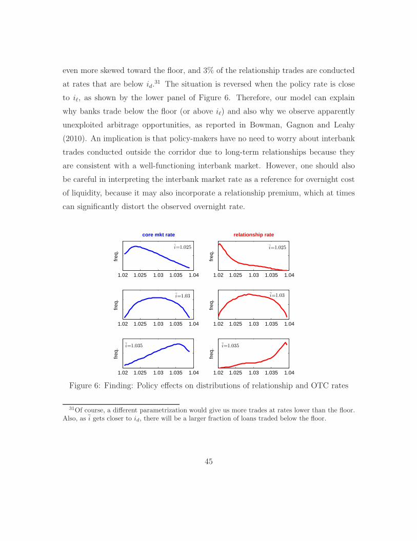
even more skewed toward the floor, and 3% of the relationship trades are conducted

at rates that are below id.31 The situation is reversed when the policy rate is close

to iℓ, as shown by the lower panel of Figure 6. Therefore, our model can explain

why banks trade below the floor (or above iℓ) and also why we observe apparently

unexploited arbitrage opportunities, as reported in Bowman, Gagnon and Leahy

(2010). An implication is that policy-makers have no need to worry about interbank

trades conducted outside the corridor due to long-term relationships because they

are consistent with a well-functioning interbank market. However, one should also

be careful in interpreting the interbank market rate as a reference for overnight cost

of liquidity, because it may also incorporate a relationship premium, which at times

can significantly distort the observed overnight rate.

1.02 1.025 1.03 1.035 1.04

core mkt rate

freq

.

i=1.025

1.02 1.025 1.03 1.035 1.04

relationship rate

freq

.

i=1.025

1.02 1.025 1.03 1.035 1.04

freq

.

i=1.03

1.02 1.025 1.03 1.035 1.04

freq

.

i=1.03

1.02 1.025 1.03 1.035 1.04

freq

. i=1.035

1.02 1.025 1.03 1.035 1.04

freq

. i=1.035

Figure 6: Finding: Policy effects on distributions of relationship and OTC rates

31Of course, a different parametrization would give us more trades at rates lower than the floor.Also, as i gets closer to id, there will be a larger fraction of loans traded below the floor.

45

6.3 Network structure

We now turn to the effect of monetary policy on the network structure. Figure 7

shows the (unweighted) flows of payment for several maintenance periods. When γ =

0, the core market is costless to access. Therefore, whether they are in a relationship

or not, S banks will enter. Therefore, after a sufficient number of maintenance

periods, all banks will have traded with one another at least once, as shown by the

left panel of Figure 7. In this case monetary policy only affects the network structure

insofar as it affects the core market tightness.

Now consider the case when accessing the core market is expensive for S banks.

We have seen that a relationship is most valuable and the number of relationships

is maximized when the policy rate is at the midpoint of the corridor. The network

structure is then as shown by the right panel of Figure 7. Since γ is large, single S

banks choose not to access the core market while S banks in a relationship will also

rely on their partners and will not access the core market. So only L banks are active

in the core market and provide intermediation for some S banks in the peripheral

market.

Finally, suppose the central bank is adopting a more accommodative policy stance

and lowers i close to id. Then, as γ is large, no S bank will access the core market;

however, a relationship becomes not so valuable, as all banks are holding enough

reserves to satisfy their reserves requirements. Therefore, single S banks have no

incentives to build a relationship, and the tiered network structure will slowly vanish

as banks are hit by the exogenous separation shock. Then the network structure

from the flow of payment will resemble the pattern shown on the middle panel of

Figure 7. 32,33

32Interestingly, this is consistent with the network change in the fed funds market as reported inBeltran, Bolotnyy and Klee (2015): “many small federal funds lenders began reducing their lendingto larger institutions in the core of the network starting in mid-2007.”

33Again, this model in some way endogenizes bank sizes: even when banks face the same shockdistribution, G = F , the L banks will appear more active in the interbank market, hence justifying

46

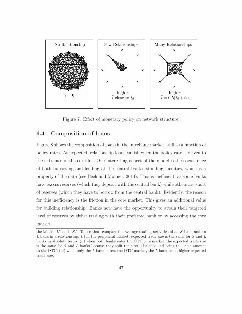
high γγ = 0

i = 0.5(id + iℓ)

No Relationship Many Relationships

high γ

i close to id

Few Relationships

Figure 7: Effect of monetary policy on network structure.

6.4 Composition of loans

Figure 8 shows the composition of loans in the interbank market, still as a function of

policy rates. As expected, relationship loans vanish when the policy rate is driven to

the extremes of the corridor. One interesting aspect of the model is the coexistence

of both borrowing and lending at the central bank’s standing facilities, which is a

property of the data (see Bech and Monnet, 2014). This is inefficient, as some banks

have excess reserves (which they deposit with the central bank) while others are short

of reserves (which they have to borrow from the central bank). Evidently, the reason

for this inefficiency is the friction in the core market. This gives an additional value

for building relationship: Banks now have the opportunity to attain their targeted

level of reserves by either trading with their preferred bank or by accessing the core

market.

the labels “L” and “S.” To see that, compare the average trading activities of an S bank and anL bank in a relationship: (i) in the peripheral market, expected trade size is the same for S and L

banks in absolute terms; (ii) when both banks enter the OTC core market, the expected trade sizeis the same for S and L banks because they split their total balance and bring the same amountto the OTC; (iii) when only the L bank enters the OTC market, the L bank has a higher expectedtrade size.

47

0%

10%

20%

30%

40%

50%

60%

70%

80%

90%

100%

0.2 0.23 0.27 0.3 0.32 0.34 0.36 0.4

CBdeposit CBloans OTCloan Relationshiploan

Figure 8: Finding: Policy effects on composition of overnight loans

6.5 Temporary liquidity expansion/contraction

Our analysis so far focuses on permanent anticipated changes in monetary policy.

We now consider a one-time unanticipated liquidity injection to the banking system.

Consider a steady-state equilibrium under a symmetric corridor (i.e., i = 3.0%).

Suppose all banks receive a surprise lump-sum reserve injection ∆m ≷ 0 from the

central bank after the liquidity sale, and receive zero injections in all subsequent

periods. This exercise captures a situation in which the central bank conducts a

temporary monetary expansion/contraction, with its commitment to restore steady-

state policy in the long run.

Crucially, the policy effects of these temporary deviations from a symmetric cor-

ridor are different from those of a permanent deviation. Table 2 reports the effects

of such intervention on the quantities and prices of interbank loans. Naturally, a

liquidity injection drives the core and relationship rates to the floor while a with-

drawal drives the rates to iℓ. More interestingly, contrary to a permanent liquidity

injection, a temporary liquidity injection does not affect the number of relationship

48

Table 2: Temporary Liquidity Expansion/ContractionRelationship loans OTC loans

∆m no. of loans avg. i loans with i < id loans with i > iℓ no. of loans avg. r−2 0.2031 1.0371 0.98% 3.15% 0.1128 1.0344−1 0.2031 1.0346 1.16% 2.86% 0.2551 1.03210 0.2031 1.0300 1.85 % 2.05% 0.4739 1.0297+1 0.2031 1.0247 2.62% 1.42% 0.2690 1.0275+2 0.2031 1.0214 3.48% 1.09% 0.1192 1.0254

loans. Figure 8 shows that a permanent deviation from a symmetric corridor al-

ways reduces the number of loans in the core and peripheral markets. A one-time

monetary expansion/contraction also reduces core market loans because the market

becomes less balanced, but the effect on relationship loans is quite different. Since

banks in a relationship are not subject to search frictions, the number of relationship

loans is unaffected. Moreover, since these policies are temporary, the relationship

premium is also unaffected. As a consequence, there remains a significant fraction

of relationship loans traded below the floor for a liquidity injection and a significant

fraction of loans traded above the ceiling for a large liquidity withdrawal.34

6.6 Moving from a floor system to a symmetric corridor

Finally we compute the transition path when the central bank moves the policy rate

from the bottom (i.e., floor system) to the midpoint of the corridor (i.e., symmetric

corridor system). The transition paths of η = 1−NL and V are plotted in Figure 9.

As in the benchmark model, there is an overshoot of relationship formation, as the

number of relationships increases immediately in response to the policy change. Af-

terwards, the number of relationships declines monotonically to its new steady value.

As discussed in the benchmark model, S banks’ value of long-term relationships also

exihibits a non-montonic time path.

34One can show that, as ∆m → ∞, OTC loans vanish but there remains a positive number ofrelationship loans. Moreover, a positive fraction of relationship loans are traded below the floor.

49

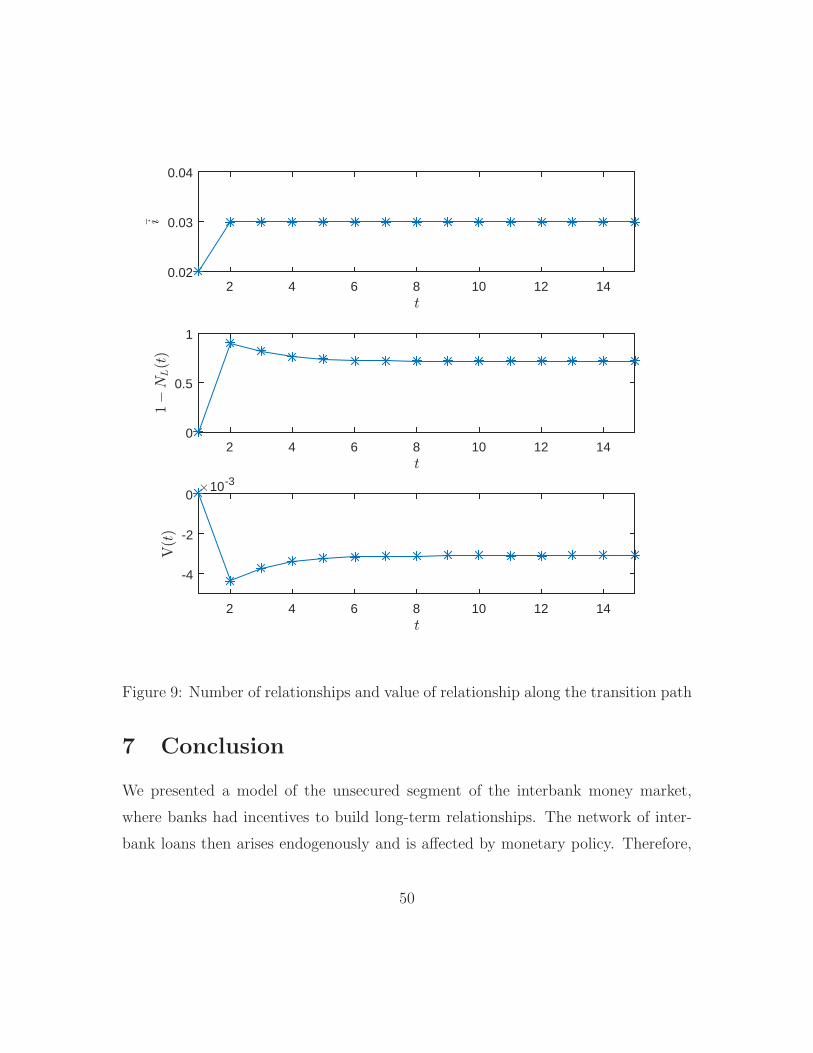
2 4 6 8 10 12 14

0.02

0.03

0.04

2 4 6 8 10 12 14

0

0.5

1

2 4 6 8 10 12 14

10-3

-4

-2

0

Figure 9: Number of relationships and value of relationship along the transition path

7 Conclusion

We presented a model of the unsecured segment of the interbank money market,

where banks had incentives to build long-term relationships. The network of inter-

bank loans then arises endogenously and is affected by monetary policy. Therefore,

50

the model sheds some light on the policy effects on the interbank network, reserve

demand, and interest rate dispersion. We derive testable implications regarding the

network structure and the composition, quantities and prices of loans. We show that

relationship can help explain some puzzling observations, such as why the floor of

the corridor is “soft.” The model is simple and tractable and, we believe, captures

some important components of the interbank market. As such, it can be a useful

tool for policy-makers, e.g., to investigate quantitatively the short-run and long-run

effects of running and “exiting” the floor system and the potential effects of various

regulatory proposals.

Of course we had to make some simplifying assumptions. For example, we could

have assumed that banks in a relationship can meet once more after the core market.

However, this would have unnecessarily complicated the analysis of trades in the core

market. More importantly, we now assume that L banks can set up a link with only

one other bank. It could be interesting to relax this assumption. Also, S banks may

have the incentive to create some relationships with each other and delegate access

to the core market to one of them, while sharing the access cost. Effectively, they

would become large, as they would each bear only a small fraction of the access cost.

We have not explored this interesting possibility here, but in the companion paper

we study an extension where any pairs of banks can form a relationship and another

extension where banks can trade in the OTC market multiple times.

A characteristics of the fed funds market is that small banks are usually cash rich

and lend to the large cash-poor banks. As Stigum and Crescenzi (2007) summarize it,

“In the fed funds market now, regional banks buy up funds from even tiny banks, use

what they need, and resell the remainder in round lots in the New York market. Thus,

the fed funds market resembles a river with tributaries: money is collected in many

places and then flows through various channels into the New York market. In essence,

the nation’s smaller banks are the suppliers of fed funds, and the larger bankers are

the buyers.” Our model obviously encompasses this case and our parametrization

51

makes full use of it by imposing two different distributions of the liquidity shocks for

the two types of banks: The distribution of shocks for the S banks has a positive

mean, while the shock for L banks has a negative mean.

Also, instead of assuming a fixed cost of entry in the core market, we could have

assumed that it is reserved for large transactions. Indeed Crescenzi and Stigum

(2007) report that “A smaller bank could, of course, shop in the brokers’ market and

try to pick up an extra, but most don’t because the amounts they sell are so small

that the cost of trying would outweigh the potential gain. Overnight on $10 million

is only $17, and that’s before the phone bill is paid.(...) The brokers’ market is really

open to only those banks that buy and sell in volume. In fed funds, round lots are $5

million, the same as the notional amount on the fed funds futures that trade at the

Chicago Board of Trade. A small bank in Iowa that wants to buy $500,000 is better

off going to its regional correspondent, since the New York brokers are not set up to

handle trades of that size.” However our fixed-cost assumption is a good assumption

for this aspect of the market, and our results would have been essentially the same.

Also, notice that, in equilibrium, trade in the core market will be relatively large,

and thus consistent with this evidence.

Finally, we have left aside credit risk as well as the juxtaposition of the unsecured

and secured segments of the money market. It is clear that credit risk will affect the

quality of long-term relationships. Also, we have seen the importance of the secured

segment during the recent financial crisis. Adding both elements to the current

model would be a natural and very interesting next step. We leave these and other

improvements for future research.

52

References

[1] Afonso, G., A. Kovner, and A. Schoar (2012). “The Importance of Trading

Relationships in the Fed Funds Market,” mimeo, Federal Reserve Bank of New

York.

[2] Afonso, G. and R. Lagos (2012). “An Empirical Study of Trade Dynamics in

the Fed Funds Market,” mimeo, Federal Reserve Bank of New York.

[3] Afonso, G. and R. Lagos (2015). “Trade Dynamics in the Market for Federal

Funds.” Econometrica 83.1: 263-313.

[4] Allen, F. and A. Babus (2009) “Networks in Finance,” in P. Kleindorfer and J.

Wind (ed.) Network-based Strategies and Competencies, 367-382.

[5] Allen, F. and G. Douglas (2000) “Financial Contagion.” Journal of Political

Economy 108, 1-33.

[6] Armantier, O. and A. Copeland (2012). “Assessing the Quality of ’Furfine-based’

Algorithms.” Staff Report 575, Federal Reserve Bank of New York.

[7] Ashcraft, A. and D. Duffie (2007). “Systemic Illiquidity in the Federal Funds

Market.” American Economic Review 97(2), 221-225.

[8] Babus, A. (2013) “Endogenous Intermediation in Over-the-Counter Markets,”

mimeo, Federal Reserve Bank of Chicago.

[9] Bech, M. and E. Atalay (2010). “The topology of the federal funds market.”

Physica A: Statistical Mechanics and its Applications 389.22: 5223-5246.

[10] Bech, M., C. Bergstrom, R. Garratt, and M. Rosvall (2014). “Mapping Change

in the Federal Funds Market.” Federal Reserve Bank of New York Staff Reports,

no. 507.

53

[11] Bech, M. and C. Monnet (2014). “Sorting in the Interbank Market,” mimeo,

Bank for International Settlements.

[12] Bech, M. and T. Keister (2012). “The Liquidity Coverage Ration and Monetary

Policy,” mimeo, Bank for International Settlements.

[13] Bech, M. and E. Klee (2011). “The Mechanics of a Graceful Exit: Interest on

Reserves and Segmentation in the Federal Funds Market.” Journal of Monetary

Economics 58, 415–431.

[14] Beltran, D., V. Bolotnyy, and E. Klee (2015). “ ’Un’-Networking: The Evolution

of Networks in the Federal Funds Market,” mimeo, Federal Reserve Board of

Governors, DC.

[15] Berentsen, A. and C. Monnet (2008). “Monetary Policy in a Channel System.”

Journal of Monetary Economics 55, 1067-1080.

[16] Berentsen, A., A. Marchesiani, and C. Waller (2011). “Floor Systems for Im-

plementing Monetary Policy: Some Unpleasant Fiscal Arithmetic.” Review of

Economic Dynamics 17(3), 523-542.

[17] Berentsen, A. and C. Waller (2011). “Price Level Targeting and Stabilization

Policy.” Journal of Money, Credit, and Banking 43(s2), 559-580.

[18] Blasques, F., F. Brauning, and I. van Lelyveld (2015). “A Dynamic Network

Model of The Unsecured Interbank Lending Market.” BIS Working Paper No.

491.

[19] Bowman, D., E. Gagnon and M. Leahy (2010). “Interest on Excess Reserves as a

Monetary Policy Instrument: The Experience of Foreign Central Banks.” Board

of Governors of the Federal Reserve System, International Finance Discussion

Papers No. 996.

54

[20] Brauning, F. and F. Fecht (2012). “Relationship Lending and Peer Monitoring:

Evidence from Interbank Payment Data,” mimeo, VU University of Amsterdam.

[21] Chang, B. and S. Zhang (2015). “Endogenous Market Making and Network

Formation,” mimeo, University of Wisconsin-Madison.

[22] Craig, B., and G. Von Peter (2014). “Interbank Tiering and Money Center

Banks.” Journal of Financial Intermediation 23.3: 322-347.

[23] Duffie, D., N. Garleanu, and L. Pedersen (2005). “Over the Counter Markets.”

Econometrica 73.6: 1815-1847.

[24] Elliott, M. L., B. Golub, and M. O. Jackson (2014). “Financial Networks and

Contagion.” American Economic Review 104.10 (2014): 3115-3153.

[25] European Central Bank (2002) “The Liquidity Management of The ECB.” ECB

Monthly Bulletin.

[26] European Central Bank (2013) “Euro Money Market Survey,” November.

[27] Ennis, H. and J. Weinberg (2013) “Over-The-Counter Loans, Adverse Selection,

and Stigma in The Interbank Market.” Review of Economic Dynamics 16, 601-

616.

[28] Furfine, C. (1999) “The Microstructure of the Federal Funds Market.” Financial

Markets, Institutions & Instruments 8(5), November.

[29] Gofman, M. (2011) “A Network-Based Analysis of Over-the-Counter Markets,”

mimeo, Wisconsin Business School.

[30] Gofman, M. (2014) “Efficiency and Stability of a Financial Architecture with

Too-Interconnected-to-Fail Institutions,” mimeo, Wisconsin Business School.

55

[31] Hamilton, J. D. (1996) “The Daily Market for Federal Funds.” Journal of Po-

litical Economy 104, 26–56.

[32] Hartmann, P., M. Manna, and A. Manzanares (2001) “The Microstructure Of

The Euro Money Market.” Journal of International Money and Finance 20(6),

895-948.

[33] Jackson, M. O. (2010) “Social and Economic Networks.” Princeton University

Press.

[34] Keister T., A. Martin and J. McAndrews (2008). “Divorcing Money from Mon-

etary Policy.” Federal Reserve Bank of New York Economic Policy Review.

[35] Klee, E., and V. Stebunovsy (2013) “Target practice: Monetary policy imple-

mentation in a post-crisis environment,” manuscript.

[36] Lagos, R., and G. Rocheteau (2009). “Liquidity in asset markets with search

frictions.” Econometrica 77.2: 403-426.

[37] Lagos, R., G. Rocheteau, and P-O. Weill (2011) “Crises and Liquidity in Over-

the-Counter Markets.” Journal of Economic Theory 146, 2169-2205.

[38] Lascelles, E. (2009). “Rate Cutting On The Sly.” TD Securities Market Musings,

May 14.

[39] Leitner, Y. (2005) “Financial Networks: Contagion, Commitment, and Private

Sector Bailouts.” Journal of Finance 60, 2925-2953.

[40] Li, Y., G. Rocheteau, and P.-O. Weill (2012) “Liquidity and the Threat of

Fraudulent Assets.” Journal of Political Economy 120, 815-846.

[41] Poole, W. (1968). “Commercial Bank Reserve Management in a Stochastic

Model: Implications for Monetary Policy.” Journal of Finance 23, 769–791.

56

[42] Rajan, R. G. (1992). “Insiders and Outsiders: The Choice Between Informed

and Arm’s-length Debt.” Journal of Finance 47(4):1367–400.

[43] Rocheteau, G. and R. Wright (2013) “Liquidity and Asset Market Dynamics.”

Journal of Monetary Economics 60, 275-294.

[44] Stigum, M. and A. Crescenzi (2007) Stigum’s Money Market, McGraw-Hill Ed-

ucation, 4th Edition.

[45] Vila, A., K. Soramaki, and P. Zimmerman (2010). “The Sterling Unsecured

Loan Market During 2006–2008: Insights From Network Theory,” manuscript.

57

Appendix

A Proof of Proposition 3

Proof. Consider a trade between an S bank and an L bank. Recall that

v3(R,L, n) = maxΠ(R)− γ, 0+ β L+R(1 + i(R))+ βv1(n).

If the S bank lends z to the L bank, its payoff is

v3(RS − z, z(1 + i), 1)

= maxΠ(RS − z)− γ, 0+ β

z(1 + i) + (RS − z)(1 + i(Rs − z))

+ βv1(1).

If it does not lend, its payoff depends on whether the L bank has been contacted or

not. If c = 1, then the L bank can credibly threaten to break up the relationship if

no trade is conducted in the current period. Therefore, the S bank’s payoff without

trade is

v3(RS, 0, 0)

= maxΠ(RS)− γ, 0+ β RS(1 + i(RS))+ βv1(0).

In this case, the trade surplus for an S bank is

v3(RS − z, z(1 + i), 1)− v3(RS, 0, 0).

In contrast, when c = 0, the relationship continues even when there is no trade in

the current period and the S bank’s payoff is

v3(RS, 0, 1)

= maxΠ(RS)− γ, 0+ β RS(1 + i(RS))+ βv1(1).

In that case, the trade surplus for an S bank is

v3(RS − z, z(1 + i), 1)− v3(RS, 0, 1).

58

As a result, the S bank’s trade surplus conditional on c is

TSS(z, i; c)

=v3(RS − z, 0, 0)− v3(RS, 0, 0) + βz(1 + i) + cβ[v1(1)− v1(0)]

=maxΠ(RS − z)− γ, 0 −maxΠ(RS)− γ, 0+ β

z(1 + i) + (RS − z)(1 + i(RS − z))−RS(1 + i(RS))

+ cβ(1− σ)[v1(1)− v1(0)].

Since an S bank cannot credibly end a relationship, the trade surplus for an L bank

with reserves RL is always

V3(RL + z, z(1 + i), 1)− V3(RL, 0, 1),

where

V3(RL + z,−z(1 + i), 1) = β(RL + z)(1 + im)− βz(1 + i) + βV1(1)

V3(RL, 0, 1) = βRL(1 + im) + βV1(1).

Hence, its surplus conditional on c is

TSL(z, i; c)

=V3(RL + z, z(1 + i), 1)− V3(RL, 0, c)

=βz(1 + im)− βz(1 + i).

Then, the total surplus from a loan of size z is

TS(z; c) = v3(RS − z, 0, 0)− v3(RS, 0, 0) + V3(RL + z, 0, 0)− V3(RL, 0, 0)

+cβ(1− σ)[v1(1)− βv1(0)]

= maxΠ(RS − z)− γ, 0 −maxΠ(RS)− γ, 0+β (RS − z)(1 + i(RS − z))−RS(1 + i(RS))+ cβ(1− σ)[v1(1)− v1(0)]

+βz(1 + im)

59

Since γ > 0 and im ∈ [id, iℓ], it is straightforward to show that Rs = argmaxz TS(z)

and hence the total surplus from the trade is

TS(RS; c) = −maxΠ(RS)−γ, 0−βRS(1+i(RS))+cβ(1−σ)[v1(1)−v1(0)]+βRS(1+im).

Setting TSL = (1− θ)TS(RS), we obtain

1 + i(RS, RL, c) = (1− θ)maxβ[1 + i(RS)]RS,−γ + β[1 + im(R)]RS

βRS

+θ[1 + im(R)] + (1− θ)cVRS

.

Therefore, the S bank will always lend z to the L bank and choose not to participate

in the core market.

60

B Value in sub-period 2

The expected value of a matched L bank with reserve holdings M before the shock

is

V2(M, 1;M)

=

ˆ

∞

−∞

ˆ

∞

−∞

Ec

[

V3(M + ε+m1 + ξ,−[1 + i(m1 + ξ, c)](m1 + ξ); 0)]

dG(ε)dF (ξ)

+β[V1(1)− V1(0)

].

=

ˆ

∞

−∞

ˆ

∞

−∞

Ec

[

β (M + ε) (1 + im(R))− β [i(m1 + ξ, c)− im(R)](m1 + ξ)]

dG(ε)dF (ξ) + βV1(1).

so that∂V2(M, 1;M)

∂M= β(1 + im(R)).

Similarly, the expected value of a matched S bank with reserve holdings m before

the shock is

v2(m1, 1;M)

=

ˆ

∞

−∞

Ec

[

v3(0, [1 + i(m1 + ξ, c)](m1 + ξ); 0)]

dF (ξ) + β [v1(1)− v1(0)] .

=

ˆ

∞

−∞

Ecβ[1 + i(m1 + ξ, c)](m1 + ξ)dF (ξ) + βv1(1).

=

ˆ

∞

−∞

β[(1− θ)maxΠ(m1 + ξ)− γ, 0+ β (m1 + ξ)(1 + i(m1 + ξ))

+θ(1 + im(R))(m1 + ξ) + βEc [cV]]dF (ξ) + βv1(1).

=

ˆ

∞

−∞

β(1 + im(R)

)(m1 + ξ)− β(1− θ)

[

Ieγ

β+ Ine

[im(R)− i(m1 + ξ)

](m1 + ξ)

]

dF (ξ)

+βEc [cV] + βv1(1).

so that, using Ie = 1 when the bank decides to enter the core market and zero

otherwise and Ine is 1 when the bank opts to stay out of the core market and zero if

61

it chooses to enter,

∂v2(m1, 1;M)

∂m1

= β(1 + im(R)

)+ β(1− θ)

ˆ

∞

−∞

Ine

[i(m1 + ξ)− im(R)

]dF (ξ)

= β(1 + im(R)

)+ β(1− θ)

ˆ

γ

β(im(R)−id)−m1

−γ

β(iℓ−im(R))−m1

[i(m1 + ξ)− im(R)

]dF (ξ)

= β(1 + im(R)

)+ β(1− θ)

ˆ

γ

β(im(R)−id)−m1

−m1

[id − im(R)

]dF (ξ) +

ˆ

−m1

−γ

β(iℓ−im(R))−m1

[iℓ − im(R)

]dF (ξ)

= β(1 + im(R)

)+ β(1− θ)

[id − im(R)

]

[

F

(

γ

β(im(R)− id

) −m1

)

− F (−m1)

]

+β(1− θ)[iℓ − im(R)

]

[

F (−m1)− F

(

−γ

β(iℓ − im(R)

) −m1

)]

Notice that if im(R) = (iℓ + id)/2 then ∂v2(m1,1;M)∂m1

= β(1 + im(R)

).

Using (7) the expected value of a single L bank holding M units of reserves before

the shock is

V2(M, 0;M) =

ˆ

∞

−∞

β[(M + ε)(1 + im(R))]dG(ε) + β(1−NS)V1(0) + βNSV1(1),

so that∂V2(M, 0;M)

∂M= β(1 + im(R))

Using (8) we can write:

v2(m0, 0;M) =

ˆ

∞

−∞

maxΠ(m+ ξ)− γ, 0+ β (m+ ξ)(1 + i(m+ ξ)) dF (ξ) + v(0).

=

ˆ

∞

−∞

Ie

[β(m0 + ξ)(1 + im(R))− γ

]+ βIne(m0 + ξ) [1 + i(m0 + ξ)] dF (ξ) + v(0)

where v(0) = maxβv1(0),−κ + NLβv1(1) + (1 − NL)βv1(0) determines the value

62

of searching when single. So

∂v2(m0, 0;M)

∂m0

=

ˆ

∞

−∞

Ieβ(1 + im(R)) + Ineβ(1 + i(m0 + ξ))dF (ξ)

= β(1 + im(R)) +

ˆ

∞

−∞

Ineβ(i(m0 + ξ)− im(R))dF (ξ)

= β(1 + im(R)) +

ˆ

γ

β(im(R)−id)−m0

−γ

β(iℓ−im(R))−m0

β(i(m0 + ξ)− im(R))dF (ξ)

= β(1 + im(R)

)+ β

[id − im(R)

]

[

F

(

γ

β(im(R)− id

) −m0

)

− F (−m0)

]

+β[iℓ − im(R)

]

[

F (−m0)− F

(

−γ

β(iℓ − im(R)

) −m0

)]

.

63

C Proof of Proposition 6

Proof. Recall that the search strategy of single S banks is given by (13). Using (12),

we have that if NS = NL (i.e., all single S banks search), then NL solves

(1− σ)N2L + σNL − σ = 0

or

N∗

L =−σ +

√

σ2 + 4(1− σ)σ

2(1− σ),

and if NS = 0 (i.e., no S banks search) then NL = 1. That is, if none of the single

S banks search, then all L banks are single. Let

Γ ≡ˆ

∞

−∞

βθ

[

Ieγ

β+ Ine

[iℓ + id

2− i(ξ)

]

ξ

]

dF (ξ)

be the expected per-period benefit of a relationship for the S bank when the interbank

market is in the midpoint of the corridor. Then

Lemma 10. If i 6= (iℓ + id)/2 then v1(1) = v1(0) so that NS = 0 and there is no

relationship. When i = (iℓ + id)/2 then either NS = N∗

L and

v1(1)− v1(0) ≥2

β[

−σ +√

σ2 + 4(1− σ)σ]κ

or NS = NS and

v1(1)− v1(0) =

[(1− σ)NS + σ

]

σ(1− σ)βκ

where NS is implicitly given by

σβ(1− σ)[(1− σ)NS + σ

]Γ

[1− β(1− σ)

[1− NS(1− θ)

]] = κ,

or NS = 0 and NL = 1, and

(1− σ)β [v1(1)− v1(0)] < κ.

64

When i 6= (iℓ + id)/2 then v1(1) = v1(0). (13) implies that NS = 0 and there is

no relationship. When i = (iℓ+ id)/2 then proposition (4) implies that m0 = m1 = 0

and v1(n) = v2(0, n; 0). Suppose first NS is interior. Since im(R) = i we have

v2(0, 0;M) =

ˆ

∞

−∞

Ie

[

βξ

(

1 +iℓ + id

2

)

− γ

]

+ βIne [1 + i(ξ)] ξdF (ξ) + v(0)

=

ˆ

∞

−∞

β

(

1 +iℓ + id

2

)

ξ − β

[

Ieγ

β+ Ine

[iℓ + id

2− i(ξ)

]

ξ

]

dF (ξ) + v(0)

where v(0) = maxβv1(0),−κ + NLβv1(1) + (1 − NL)βv1(0) determines the value

of searching when single. Also

v2(0, 1;M) =

ˆ

∞

−∞

β

(

1 +iℓ + id

2

)

ξ − β(1− θ)

[

Ieγ

β+ Ine

[iℓ + id

2− i(ξ)

]

ξ

]

dF (ξ)

+ βEc [cV] + βv1(1).

Therefore

v1(1)− v1(0) = v2(0, 1, 0)− v2(0, 0, 0)

= Γ + βEc [c(1− θ)V] + βv1(1)− v(0)

= Γ− βEc [c(1− θ)(1− σ)[v1(1)− v1(0)]]

+βv1(1)−maxβv1(0),−κ+NLβv1(1) + (1−NL)βv1(0)

and using v1(1) = (1− σ)v1(1) + σv1(0) we obtain,

v1(1)− v1(0) = Γ− βEc [c(1− θ)(1− σ)[v1(1)− v1(0)]]

+minβ(1− σ)[v1(1)− v1(0)], κ+ (1−NL) β(1− σ)[v1(1)− v1(0)]= Γ− βEc [c(1− θ)(1− σ)[v1(1)− v1(0)]] + β(1− σ)[v1(1)− v1(0)]

where the last equality follows from the fact that the solution for NS is interior. In

this case, Ec [c] = NS and

v1(1)− v1(0) =Γ

1− β(1− σ) [1−NS(1− θ)].

65

Hence, to find NS we need to solve

NLβ(1− σ)[v1(1)− v1(0)] = κ.

Using (12) evaluated at NS, we obtain

σ(1− σ)β[(1− σ)NS + σ

] [v1(1)− v1(0)] = κ,

and using v1(1)− v1(0) we obtain

σβ(1− σ)[(1− σ)NS + σ

]Γ

[1− β(1− σ)

[1− NS(1− θ)

]] = κ, (C.1)

which implicitly defines NS. Also, since

NL =σ

(1− σ)NS + σ

we getNLβ(1− σ)

[1− β(1− σ)

[1− NS(1− θ)

]]Γ = κ,

When all single S banks prefer to search and the solution NS is not interior, then

v1(1)− v1(0) = Γ− βEc [c(1− θ)(1− σ)[v1(1)− v1(0)]]

+κ+ (1−NL)β(1− σ)[v1(1)− v1(0)]

= Γ− βNS(1− θ)(1− σ)[v1(1)− v1(0)]

+κ+ (1−NL)β(1− σ)[v1(1)− v1(0)]

=Γ + κ

1− β(1− σ) (1−NL −NS(1− θ)).

This equilibrium exists if and only if

N∗

L(1− σ)βΓ + κ

1 − β(1− σ) (1−N∗

L −N∗

S(1− θ))> κ

orN∗

L(1− σ)β

[1− β(1− σ) (1−N∗

S(1− θ))]Γ > κ.

66

Finally, if no single banks search (i.e., NS = 0), then

v1(1)− v1(0) =Γ

1− β(1− σ).

This equilibrium exists if and only if

(1− σ)β

1− β(1− σ)Γ < κ.

It is clear that the parameter space defines three distinct and non-overlapping

but connected regions. In each of these regions the equilibrium is well defined and

unique. So the equilibrium is unique.

67

D Proof of Lemma 7

Proof. Relationship benefits

Γ ≡ˆ

∞

−∞

βθ

[

Ieγ

β+ Ine

[iℓ + id

2− i(ξ)

]

ξ

]

dF (ξ)

= βθ

[ˆ

∞

R+

γ

β+

ˆ R−

−∞

γ

β+

ˆ R+

R−

[iℓ + id

2− i(ξ)

]

ξ

]

dF (ξ)

= βθ

[

γ

β

[

1− F (R+)]

+γ

βF (R−) +

ˆ R+

0

[iℓ + id

2− id

]

ξ +

ˆ 0

R−

[iℓ + id

2− iℓ

]

ξ

]

dF (ξ)

= βθ

[

γ

β

[

1− F (R+)]

+γ

βF (R−) +

[iℓ − id

2

](ˆ R+

0

ξ −ˆ 0

R−

ξ

)

dF (ξ)

]

When the variance of the shock ξ increases, S banks will find it profitable to enter

more often. Therefore, more weight is placed on γ/β relative to the other component

of Γ, which is smaller than γ/β. Hence, Γ increases in the variance of the shock ξ.

Also,

1

βθdΓ = −γ

βf(R+)dR+ +

[iℓ + id

2− id

]

R+f(R+)dR+

= −γ

βf(R+)dR+ +

γ

β

[iℓ − id

2

]1

(im(R)− id

)f(R+)dR+

= −γ

β

[

1−[iℓ − id

2

]1

(im(R)− id

)

]

f(R+)dR+

and

1

βθdΓ =

γ

βf(R−)dR− −

[iℓ + id

2− iℓ

]

R−f(R−)dR−

=γ

βf(R−)dR− − γ

β

[iℓ − id

2

]1

(iℓ − im(R)

)f(R−)dR−

=γ

β

[

1−[iℓ − id

2

]1

(iℓ − im(R)

)

]

f(R−)dR−.

68

Hence, assuming that f(x) converges fast enough to zero as x → ∞ or −∞,

∂Γ

∂R+=

0 if R ≥ 0

−βθ γ

2βf(R+)dR+ if R < 0

while∂Γ

∂R−=

0 if R ≤ 0

βθ γ

2βf(R−)dR− if R > 0

.

Therefore, if iℓ − id increases, then

∂Γ

∂(iℓ − id)

∣∣∣i=

iℓ+id2

= βθ (iℓ − id)

(ˆ R+

0

ξ −ˆ 0

R−

ξ

)

dF (ξ) > 0

∂Γ

∂(iℓ − id)

∣∣i=iℓ

= −βθγ

2βf(R+)

∂R+

∂(iℓ − id)+ βθ (iℓ − id)

(ˆ R+

0

ξ −ˆ 0

R−

ξ

)

dF (ξ) > 0

∂Γ

∂(iℓ − id)

∣∣i=id

= βθγ

2βf(R−)

∂R−

∂(iℓ − id)+ βθ (iℓ − id)

(ˆ R+

0

ξ −ˆ 0

R−

ξ

)

dF (ξ) > 0.

Hence Γ (measuring the gains from relationships) increases as the corridor size in-

creases. Also

∂Γ

∂γ

∣∣∣i=

iℓ+id2

= θ[

1− F (R+) + F (R−)]

> 0

∂Γ

∂(iℓ − id)

∣∣i=iℓ

= −βθγ

2βf(R+)

1

β (iℓ − id)+ θ

[

1− F

(γ

β (iℓ − id)

)]

∂Γ

∂(iℓ − id)

∣∣i=id

= −βθγ

2βf(R−)

1

β (iℓ − id)+ θF

( −γ

β (iℓ − id)

)

and Γ increases with γ if and only if

2 >γ

β (iℓ − id)

f(

γ

β(iℓ−id)

)

[

1− F(

γ

β(iℓ−id)

)] .

Finally NS is implicitly given by

σβ(1− σ)[(1− σ)NS + σ

]Γ

[1− β(1− σ)

(1− NS(1− θ)

)] = κ.

The LHS is decreasing in NS and increasing in Γ and θ. Hence NS is increasing in

iℓ − id, θ, and the variance of the shock ξ, and it is decreasing in κ.

69

E Exiting from the floor

In section (5.3), we derive the transition path when the central bank announces at

time T it will exit from the floor at T + 1, and when single S banks strictly prefer

to search. Here we consider the case when single S banks are indifferent between

searching and not for all t ≥ T (for some T ). To solve for the transition path, notice

that

v1(1, t)− v1(0, t) = v2(0, 1, 0, t)− v2(0, 0, 0, t)

= Γ + βEc [c(1− θ)Vt+1] + βv1(1, t+ 1)− v(0, t)

= Γ− βEc [c(1− θ)(1− σ)[v1(1, t+ 1)− v1(0, t+ 1)]] + βv1(1, t+ 1)

−maxβv1(0, t+ 1),−κ +NL(t)βv1(1, t+ 1) + (1−NL(t))βv1(0, t+ 1)

(again, single banks search at t but only get the benefit at t+1, so what matters is the

number of available L banks at date t) and using v1(1, t) = (1−σ)v1(1, t)+ σv1(0, t)

and indifference to search,

v1(1, t)− v1(0, t) (E.1)

= Γ + β(1− σ)[v1(1, t+ 1)− v1(0, t+ 1)] 1− Ec [c(1− θ)]

The indifference condition gives us

βv1(0, t+ 1) = −κ +NL(t)βv1(1, t+ 1) + (1−NL(t))βv1(0, t+ 1)

and using the expression for v1(1, t+ 1), we get

v1(1, t+ 1)− v1(0, t+ 1) =κ

β(1− σ)NL(t).

Replacing this expression in (E.1), as well as Ec[c] = NS(t), we obtain

v1(1, t)− v1(0, t) = Γ +κ

NL(t)1−NS(t)(1− θ) .

70

Since we assumed that single banks are always indifferent to searching after date T ,

we also have

v1(1, t)− v1(0, t) =κ

β(1− σ)NL(t− 1).

Combining the last two equations and rearranging terms, we obtain a first difference

equation

NS(t) =1

κ(1− θ)

[

ΓNL(t) + κ− κNL(t)

β(1− σ)NL(t− 1)

]

,

and the law of motion for NL(t+ 1) gives us a second,

NL(t + 1) = 1− [(1−NL(t))(1− σ) +NL(t)NS(t)(1− σ)] .

These two difference equations define a second-order difference equation for NL(t):

NL(t+1) = 1− (1−σ)

[

1−NL(t) +NL(t)

κ(1− θ)

[

ΓNL(t) + κ− κNL(t)

β(1− σ)NL(t− 1)

]]

,

from which we obtain the transition path to the new steady state.

71