Regularity of the Bergman Projection on Variants of the

Washington University in St. LouisWashington University Open Scholarship

Arts & Sciences Electronic Theses and Dissertations Arts & Sciences

Spring 5-15-2015

Regularity of the Bergman Projection on Variantsof the Hartogs TriangleLiwei ChenWashington University in St. Louis

Follow this and additional works at: https://openscholarship.wustl.edu/art_sci_etds

Part of the Mathematics Commons

This Dissertation is brought to you for free and open access by the Arts & Sciences at Washington University Open Scholarship. It has been acceptedfor inclusion in Arts & Sciences Electronic Theses and Dissertations by an authorized administrator of Washington University Open Scholarship. Formore information, please contact [email protected].

Recommended CitationChen, Liwei, "Regularity of the Bergman Projection on Variants of the Hartogs Triangle" (2015). Arts & Sciences Electronic Theses andDissertations. 461.https://openscholarship.wustl.edu/art_sci_etds/461

https://openscholarship.wustl.edu?utm_source=openscholarship.wustl.edu%2Fart_sci_etds%2F461&utm_medium=PDF&utm_campaign=PDFCoverPages

https://openscholarship.wustl.edu/art_sci_etds?utm_source=openscholarship.wustl.edu%2Fart_sci_etds%2F461&utm_medium=PDF&utm_campaign=PDFCoverPages

https://openscholarship.wustl.edu/art_sci?utm_source=openscholarship.wustl.edu%2Fart_sci_etds%2F461&utm_medium=PDF&utm_campaign=PDFCoverPages

https://openscholarship.wustl.edu/art_sci_etds?utm_source=openscholarship.wustl.edu%2Fart_sci_etds%2F461&utm_medium=PDF&utm_campaign=PDFCoverPages

http://network.bepress.com/hgg/discipline/174?utm_source=openscholarship.wustl.edu%2Fart_sci_etds%2F461&utm_medium=PDF&utm_campaign=PDFCoverPages

https://openscholarship.wustl.edu/art_sci_etds/461?utm_source=openscholarship.wustl.edu%2Fart_sci_etds%2F461&utm_medium=PDF&utm_campaign=PDFCoverPages

mailto:[email protected]

WASHINGTON UNIVERSITY IN ST. LOUIS

Department of Mathematics

Dissertation Examination Committee:

Steven G. Krantz, Chair

Carl M. Bender

Quo-Shin Chi

Renato Feres

Xiang Tang

Regularity of the Bergman Projection on Variants of the Hartogs Triangle

by

Liwei Chen

A dissertation presented to the

Graduate School of Arts & Sciences

of Washington University in

partial fulfillment of the

requirements for the degree

of Doctor of Philosophy

May 2015

St. Louis, Missouri

Table of Contents

Page

Acknowledgments . . . . . . . . . . . . . . . . . . . . . . . . . . . . . . . . . . . . iv

ABSTRACT OF THE DISSERTATION . . . . . . . . . . . . . . . . . . . . . . . vi

1 Introduction . . . . . . . . . . . . . . . . . . . . . . . . . . . . . . . . . . . . 1

1.1 Setup and Background History . . . . . . . . . . . . . . . . . . . . . . . 1

1.2 Problems and Results . . . . . . . . . . . . . . . . . . . . . . . . . . . . . 3

1.3 Outline and Organization . . . . . . . . . . . . . . . . . . . . . . . . . . 13

1.4 Future Directions . . . . . . . . . . . . . . . . . . . . . . . . . . . . . . . 15

1.4.1 The two-weight inequality . . . . . . . . . . . . . . . . . . . . . . 15

1.4.2 Non-smooth domains . . . . . . . . . . . . . . . . . . . . . . . . . 15

1.4.3 Smooth domains . . . . . . . . . . . . . . . . . . . . . . . . . . . 16

1.4.4 Biholomorphic mappings . . . . . . . . . . . . . . . . . . . . . . . 16

2 The Notion of Inflation . . . . . . . . . . . . . . . . . . . . . . . . . . . . . 18

2.1 Preliminaries and Basic Definitions . . . . . . . . . . . . . . . . . . . . . 18

2.2 The Inflation Theorem . . . . . . . . . . . . . . . . . . . . . . . . . . . . 19

3 The Lp Regularity . . . . . . . . . . . . . . . . . . . . . . . . . . . . . . . . 24

3.1 The Punctured Disk . . . . . . . . . . . . . . . . . . . . . . . . . . . . . 24

3.2 The Hartogs Triangle . . . . . . . . . . . . . . . . . . . . . . . . . . . . . 34

3.3 The n-dimensional Hartogs Triangle . . . . . . . . . . . . . . . . . . . . . 35

4 The Two-weight Inequality . . . . . . . . . . . . . . . . . . . . . . . . . . 39


4.2 The Properties of the Operator E . . . . . . . . . . . . . . . . . . . . . . 41

4.3 Analysis on Variants of Ap Class . . . . . . . . . . . . . . . . . . . . . . . 44

4.4 Proof of Theorem 6. . . . . . . . . . . . . . . . . . . . . . . . . . . . . . 48

5 A Wider Class of Weights . . . . . . . . . . . . . . . . . . . . . . . . . . . 53

5.1 Alternative Proof of Theorem 2 and Its Extension . . . . . . . . . . . . . 53

5.2 A Two-weight Estimate on the Hartogs Triangle . . . . . . . . . . . . . . 61

6 More Analysis on the A+p (R2

+) Class . . . . . . . . . . . . . . . . . . . . . 63


6.2 Properties of the Special Maximal Function Operator . . . . . . . . . . . 65

7 Twisted-Weighted Projections . . . . . . . . . . . . . . . . . . . . . . . . 74

ii

Page


7.2 The Lp Regularity . . . . . . . . . . . . . . . . . . . . . . . . . . . . . . 76

8 The Lp Sobolev Regularity . . . . . . . . . . . . . . . . . . . . . . . . . . . 79


8.2 Transfer to the Product Model . . . . . . . . . . . . . . . . . . . . . . . . 81

8.3 Convert the Differential Operators on D∗ . . . . . . . . . . . . . . . . . . 83

8.4 Proof of Theorem 13 . . . . . . . . . . . . . . . . . . . . . . . . . . . . . 86

8.5 Generalization to n-dimensional Hartogs Triangle . . . . . . . . . . . . . 91

References . . . . . . . . . . . . . . . . . . . . . . . . . . . . . . . . . . . . . . . . 94

iii

Acknowledgments

I would like to express my sincerest gratitude and appreciation to my thesis advisor,

Professor Steven G. Krantz, whose guidance taught me how to become a mathemati-

cian. I am also greatly thankful to his constant encouragement, support and enlightening

discussions on my research for all these years in Washington University in St. Louis.

I would like to give my greatest thanks to Professor Quo-Shin Chi, Professor Renato

Feres, and Professor Xiang Tang for their guidance on my graduate studies.

I would like to thank Professor Carl M. Bender from the Physics Department for being

part of my dissertation committee.

I would like to thank Professor Emil Straube from Texas A&M University for very

helpful comments and suggestions on my thesis work.

I would like to thank Professor Shiu-chun Wong from Zhejiang University for his

guidance on my early stage mathematics studies.

I am grateful to my parents and my friends for always being with me.

Last but not least, my thanks to Yiwen for her endless love and support, especially

on my toughest days.

iv

Dedicated to My Family.

v

ABSTRACT OF THE DISSERTATION

Regularity of the Bergman Projection on Variants of the Hartogs Triangle

by

Liwei Chen

Doctor of Philosophy in Mathematics,

Washington University in St. Louis, 2015.

Professor Steven G. Krantz, Chair

The Bergman projection is the orthogonal projection from the space of square inte-

grable functions onto the space of square integrable holomorphic functions on a domain.

Initially, the projection is defined on the L2 space, but its behavior on other function

spaces, e.g. Lp, Sobolev and Holder spaces, is of considerable interest.

In this dissertation, we focus on the Hartogs triangle which is a classical source of

counterexamples in several complex variables, and generalize it to higher dimensions.

We investigate the Lp mapping properties of the weighted Bergman projections on these

Hartogs domains. As applications, we obtain the Lp regularity of the twisted-weighted

Bergman projections and the weighted Lp Sobolev regularity of the ordinary Bergman

projection on the corresponding domains.

vi

1. Introduction

1.1 Setup and Background History

The Bergman theory has been a seminal part of geometric analysis and partial dif-

ferential equations since its invention by Stefan Bergman in 1922. It is based on a very

simple idea: suppose Ω is a domain in Cn; the set of square integrable holomorphic func-

tions on Ω, denoted by A2(Ω), forms a closed subspace of the Hilbert space L2(Ω). The

Bergman projection associated to Ω, is the orthogonal projection

B : L2(Ω)→ A2(Ω),

which has an integral representation

B(f)(z) =

∫Ω

B(z, ζ)f(ζ) dV (ζ),

for all f ∈ L2(Ω) and z ∈ Ω. Here the function B(z, ζ) defined on Ω×Ω is the Bergman

kernel.

Different types of regularity of the Bergman projection are of particular interest.

When Ω is bounded, smooth, and strongly pseudoconvex (or weakly pseudoconvex with

additional regularity properties on the boundary, e.g. finite type, property (P), and etc.),

the regularity of B in W k(Ω) and hence in C∞(Ω) have been intensively studied through

the literature.1 See, for example, [Str10] and references therein for details.

1Here the Sobolev space W k(Ω) = L2k(Ω), and for the definition of Lpk(Ω), see Chapter 8.

1

As well as the regularity in W k(Ω), the regularity of B in Lpk(Ω) and the Holder esti-

mates also have been considerably studied for many years. We mention some important

results here. In [PS77], Phong and Stein dealt with bounded smooth strongly pseudocon-

vex domains by applying the estimates of the Bergman kernel in [Fef74]. In [NRSW89],

[MS94] and [CD06], the corresponding authors studied smoothly bounded pseudoconvex

domains of finite type under additional assumptions. In [KR14], Khanh and Raich con-

sidered smoothly bounded pseudoconvex domains satisfying f -property, hence obtained

the regularity for the finite type case and a class of domains of infinite type.

There are also results for irregularity of B in Lpk(Ω) when the underlying domains are

smooth and bounded, see [Bar84,Bar92,Chr96,BS12], and regularity in Lp(Ω) when the

underlying domains are only assumed to be C2 smooth and bounded, see [LS12]. From

these, we see besides the smoothness and boundedness of the underlying domain, we need

additional regular assumption on the boundary.

When dealing with non-smooth domains, in [KP07] and [KP08], Krantz and Peloso

show that the Bergman projection for the two dimensional non-smooth worm domain is

bounded only when p is in a range depending on the winding of the domain. Even in a

planar domain, we cannot expect that the Lp regularity holds for all p ∈ (1,∞), and the

A+p class in some sense interprets the regularity condition on the boundary, see [LS04],

[Zey13], and Chapter 4 for details.2

2For the definition of A+p , see Chapter 4.

2

1.2 Problems and Results

In this dissertation, we study a class of bounded Hartogs domains which are variants

of the Hartogs triangle3

H = (z1, z2) ∈ C2 : |z1| < |z2| < 1.

To be precise, for j = 1, . . . , l, let Ωj be a smooth bounded domain in Cmj with a

biholomorphic mapping φj : Ωj → Bmj between Ωj and the unit ball Bmj in Cmj . We

use the notation zj to denote the jth mj-tuple in z′ ∈ Cm1+···+ml , that is z′ = (z1, . . . , zl).

Let m = m1 + · · · + ml ≥ 1, d = n −m ≥ 1, and z = (z′, z′′) where z′′ ∈ Cd, we define

the n-dimensional Hartogs triangle by

Hnφj

= z ∈ Cn : max1≤j≤l

|φj(zj)| < |z′′1 | < |z′′2 | < · · · < |z′′d | < 1. (1.1)

When m = 1, n = 2, and φ1 is the identity map, we obtain the classical Hartogs triangle.

Example 1 For nontrivial examples, we can take φj to be nonsingular linear mappings.

When n = 4, l = 2, m1 = 1, m2 = 2, φ1(z1) = 2z1 − 1, and φ2(z2, z3) =(z2 + 1

2z3, z3

),

we obtain a bounded domain which is the intersection of two unbounded domains,z ∈ C4 : |2z1 − 1|2 < |z4|2 < 1,

∣∣∣∣z2 +1

2z3

∣∣∣∣2 + |z3|2 < |z4|2 < 1

.

We can also take φj to be nonlinear; then we may obtain other types of domains.

When n = 3, l = 1, m1 = 2, and φ1(z1, z2) =(

z1z2−10

, 3z2 + 1), the domain becomes

z ∈ C3 :

∣∣∣∣ z1

z2 − 10

∣∣∣∣2 + |3z2 + 1|2 < |z3|2 < 1

.

By this consideration, the domains Hnφj

can be a large class of bounded Hartogs

doamins.3It should be mentioned that, there are several people who recently care about the regularity of theBergman projection on the Hartogs triangle, see [CS13] and [CZ14] for related results.

3

It is well known that the topological closure of H does not possess a Stein neighborhood

basis, and the solution to the ∂-equation on H is not globally regular. We cannot expect

the Lp regularity of Bergman projection on these variants of the Hartogs triangle to

behave very well. A first question is the following.

Question 1 Determine the exact range for p, so that the Bergman projection on Hnφj

is

Lp bounded.

To answer this question, we have the following theorem.

Theorem 1 The Bergman projection BHnφj on Hnφj

is bounded on Lp(Hnφj

)if and only if

p is in the range(

2nn+1

, 2nn−1

).

It is quite interesting that the boundedness range for p does not depend on m and

φj, but only on the dimension n. For the classical Hartogs triangle, taking n = 2, we

see the Bergman projection on the Hartogs triangle is Lp bounded if and only if p ∈(

43, 4).

Then we may ask the following natural question.

Question 2 When we look at some weighted space of the (n-dimensional) Hartogs trian-

gle, can we obtain the Lp regularity of the weighted Bergman projection for a larger range

of p?

The answer is affirmative. Note that, for the classical Hartogs triangle, the boundary

at (0, 0) is not even Lipschitz, and this singularity may blow things up. A natural way

to control boundary behavior of the singularity is the use of weights which measure the

distance from the points near the boundary to the singularity at the boundary. Since on

the Hartogs triangle we have |z2| < |z| <√

2 |z2| where z = (z1, z2) ∈ H, it is reasonable

to consider a weight of the form |z2|s′, for some s′ ∈ R.4

4See Chapter 2 for detailed definitions of weighted space and the weighted Bergman projection.

4

Before stating the results, we first consider the punctured disk D∗ = D \ 0, with

weight µ(z) = |z|s′, where z ∈ D∗ and s′ ∈ R.

Theorem 2 For s′ ∈ R with the unique expression s′ = s+2k, where k ∈ Z and s ∈ (0, 2],

let Bs′ be the weighted Bergman projection on the space (D∗, µ), where µ(z) = |z|s′.

(a) For s′ ∈ (0,∞), Bs′ is Lp(µ) bounded if and only if p ∈(s+2k+2s+k+1

, s+2k+2k+1

).

(b) For s′ ∈ [−3, 0], Bs′ is Lp(µ) bounded for p ∈ (1,∞).

(c) For s′ ∈ (−4,−3), with k = −2 and s ∈ (0, 1), Bs′ is Lp(µ) bounded if and only if

p ∈(2− s, 2−s

1−s

).

(d) When s′ = −4, B−4 is Lp(µ) bounded for p ∈ (1,∞).

(e) For s′ ∈ (−∞,−4), Bs′ is Lp(µ) bounded if and only if p ∈(s+2k+2k+1

, s+2k+2s+k+1

).

By the notion of inflation,5 one obtains the following result which improves the clas-

sical case in Theorem 1.

Theorem 3 For s′ ∈ [0,∞) with the unique expression s′ = s + 2k, where k ∈ Z and

s ∈ (0, 2], let λ(z) = |z2|s′, where z ∈ H. The weighted Bergman projection Bλ on the

weighted space (H, λ) is Lp(H, λ) bounded if and only if p ∈(s+2k+4s+k+2

, s+2k+4k+2

).

If we allow the weight λ on H to be unbounded, then we can obtain another result.

Theorem 4 Given any p0 ∈ [1, 2) with its conjugate exponent p′0, let λ(z) = |z2|−(p0+4),

where z ∈ H. Then the weighted Bergman projection Bλ on the weighted space (H, λ) is

Lp(H, λ) bounded if and only if p ∈ (p0, p′0).

5See Chapter 2 for details.

5

We can apply the same technique several times to obtain the result of the n-dimensional

Hartogs triangle, which give a full answer to the second question.

Theorem 5 Using the notation as in (1.1), let λ(z) = |z′′1 |s1 · · · |z′′d |

sd, where z ∈ Hnφj

and s1, . . . , sd ∈ R. Let Bs′ be as in Theorem 2. Then the weighted Bergman projection

on(Hnφj, λ)

is Lp(λ) bounded if and only if each of the following projections

B2m+s1 , B2m+s1+s2+2, · · · , B2m+s1+···+sd+2(d−1)

is Lp bounded on the corresponding weighted space.

In other words, assume that p > 1 and for j = 1, 2, . . . , d we let Ij be one of the

intervals for p in Theorem 2, so that the jth projection above is Lp bounded if and only if

p ∈ Ij. Then the weighted Bergman projection on(Hnφj, λ)

is Lp(λ) bounded if and only

if p ∈ ∩Ij.

After considering some particular weights on the underlying domains, one may ask

another natural question.

Question 3 Can we obtain the Lp regularity of the weighted Bergman projection on the

Hartogs triangle for a wider class of weights rather than some power of the norm of the

variable?

The answer is partly affirmative. Follow Zeytuncu’s idea in [Zey13], and using the sin-

gular integral approach due to Lanzani and Stein in [LS04], we can consider the weighted

space (D∗, µ), where µ(z) = |z|s′|g(z)|2, s′ ∈ R, and g is a non-vanishing holomorphic

function on the unit disk. Note that, by applying a Mobius transform, the isolated pole

or zero indeed can be any point in the unit disk.

6

The key observation is that the weighted Bergman kernel Bs′(z, ζ) associated to(D∗, |z|s

′ ), can be expressed as a ”homotopy” between two weighted Bergman kernels

Bs′(z, ζ) =s

2B2k+2(z, ζ) +

(1− s

2

)B2k(z, ζ)

for (z, ζ) ∈ D∗ × D∗, where s′ = s + 2k, k ∈ Z and s ∈ (0, 2]. Then, after applying the

Cayley transform ϕ : R2+ → D, where ϕ(z) = i−z

i+z, one arrives at different types of the

following two-weight inequality on the upper half plane

∫R2+

∣∣∣BR2+

(f)(z)∣∣∣p µ1(z) dV (z) ≤ C

∫R2+

|f(z)|p µ2(z) dV (z), (1.2)

where µ1 and µ2 are two weights on R2+ and

BR2+

(f)(z) =1

π

∫R2+

−f(w) dV (w)

(z − w)2

is the Bergman projection on the upper half plane.6

This observation leads to an extremely interesting and elegant theory in harmonic

analysis. Note that the operator BR2+

has a similar expression as the so-called Hilbert

integral

H(f)(x) =

∫ ∞0

f(y) dy

x+ y,

where x > 0, see [PS86a,PS86b] for further details. Both BR2+

and H, although not sin-

gular at the diagonal line, have a very close relation with the general Calderon-Zygmund

singular integrals, see [LS04]. In potential theory and classical harmonic analysis, it is of

particular interest to obtain a weighted Lp estimate of a singular integral for some weight

on the underlying domain. In the 1970s, Muckenhoupt introduced the Ap class to show

6We should point out that, initially the underlying domain is R2+ \ i. However, once we extend the

corresponding weights on R2+ \ i to R2

+, then the validity of (1.2) over R2+ \ i and R2

+ are equivalent.See arguments in Chapter 5.

7

that a necessary and sufficient condition for a general singular integral being weighted Lp

bounded is the weight satisfying the Ap condition.7

In view of the one-weight case in [LS04], we have the following conjecture.

Conjecture 1 For p > 1, if the two weights µ1 and µ2 satisfy (µ1, µ2) ∈ A+p (R2

+), then

(1.2) holds for some C > 0.

By considering the results in [Neu83], the ”power-bump” condition is also of interest.

Conjecture 2 For p > 1, if the two weights µ1 and µ2 satisfy (µr1, µr2) ∈ A+

p (R2+) for

some r > 1, then (1.2) holds for some C > 0.

Although the validity of Conjecture 1 and Conjecture 2 will make the whole theory

neater and more elegant, we have the following partial result which is sufficient for our

application.

Theorem 6 For p > 1, suppose that µ1 and µ2 are two weights such that cµ1 ≥ µ2 for

some c > 0. Then (1.2) holds for some C > 0 if and only if (µ1, µ2) ∈ A+p (R2

+).

By using different weights in (1.2) and applying Theorem 6, we extend Theorem 2 to

a wider class of weights.

Theorem 7 Assume that p > 1. Let µ(z) = |z|s′|g(z)|2, where g is a non-vanishing

holomorphic function on D and s′ ∈ R. Suppose the weighted Bergman projection B|g|2

on(D, |g|2

)is Lp

(|g|2)

bounded, and suppose the weighted Bergman projection Bs′ on(D∗, |z|s

′ )is Lp

(|z|s

′ )bounded. Then the weighted Bergman projection Bµ on (D∗, µ) is

Lp(µ) bounded.

7See Chapter 4 for detailed definitions of variants of Ap condition.

8

Moreover, suppose B|g|2 is Lp(|g|2)

bounded if and only if p ∈ (p0, p′0) for some p0 ≥ 1

and suppose Bs′ is Lp(|z|s

′ )bounded if and only if p ∈ (p1, p

′1) for some p1 ≥ 1 as

in Theorem 2. If (p1, p′1) ⊂ (p0, p

′0) properly, then Bµ is Lp(µ) bounded if and only if

p ∈ (p1, p′1).

Example 2 As in [Zey13], if we take g(z) = (z−1)t for some t > 0, then we see (p0, p′0) =(

2t+2t+2

, 2t+2t

). By Theorem 2, when s′ ∈ (0,∞), we have (p1, p

′1) =

(s+2k+2s+k+1

, s+2k+2k+1

). So

Bµ is Lp(µ) bounded if p ∈(

2t+2t+2

, 2t+2t

)⋂ (s+2k+2s+k+1

, s+2k+2k+1

).

To answer the third question, for z ∈ H we take λ(z) = |z2|s′−2 |g(z2)|2, where g is

any non-vanishing holomorphic function on D, then we have the following result.

Theorem 8 Assume that p > 1. Let λ be as above, and let p0, p1 be as in Theorem 7.

Then the weighted Bergman projection Bλ on (H, λ) is Lp(λ) bounded if p ∈ (p0, p′0) ∩

(p1, p′1). In addition, if (p1, p

′1) ⊂ (p0, p

′0) properly, then Bλ is Lp(λ) bounded if and only

if p ∈ (p1, p′1).

Again by inflation, we can apply the same technique several times to obtain a similar

result for the n-dimensional Hartogs triangle. But we will skip this part here, since there

are no new ideas.

In (1.2), we deal with two weights. Then one may ask whether we can do the same

thing for the Bergman projection on the Hartogs triangle.

Question 4 Can we also obtain the Lp regularity of the (weighted) Bergman projection

mapping from one (weighted) space to the other?

The answer is, of course, yes. We can consider the Lp regularity of the weighted

Bergman projection BH,s′ on(H, |z2|s

′ )mapping from Lp

(H, |z2|s

′ )to Lp

(H, |z2|t

)for

some t ∈ R. For simplicity, we focus on the case s′ = 2k + 2 ≥ 0, for k ∈ Z.

9

Theorem 9 Suppose that BH,2k+2 is the weighted Bergman projection on the weighted

space(H, |z2|2k+2 ). Assume p > 1 and k ≥ −1. Then, for t ≤ 2k + 2, BH,2k+2 is Lp

bounded from Lp(H, |z2|2k+2 ) to Lp

(H, |z2|t

)if and only if p ∈

(2k+6k+4

, t+4k+2

). For t > 2k+2,

BH,2k+2 is bounded from Lp(H, |z2|2k+2 ) to Lp

(H, |z2|t

)if p ∈

(2k+6k+4

, 2k+6k+2

)⋃ (t+4k+4

, t+4k+2

).

When applying the two-weight inequality (1.2), we can also consider a wider class of

weights |z2|s′|g(z2)|2 rather than |z2|s

′, where z = (z1, z2) ∈ H and g is a non-vanishing

holomorphic function on D. Indeed, if we restrict ourself to the weighted Bergman pro-

jection BH,s′ on(H, |z2|s

′ ), we can consider the Lp regularity of the BH,s′ mapping from

Lp(H, |z2|s

′ )to Lp(H, µ) for a more general weight µ satisfying the corresponding A+

p con-

ditions. On the other hand, one may also consider a weight of the form µ(z) = |z1|s′′|z2|s

′.

In this case, we have to consider once more the weighted space(D, |z|s

′′ ). The statements

of these variants are almost the same, and the arguments involve no new ideas, so we will

skip them.

As we have already seen, the two-weight inequality (1.2) has many interesting appli-

cations. In order to prove Conjecture 1 and Conjecture 2, we need a better understanding

of the A+p class. Based on the results in [Muc72,Neu83] and [Ste93, Chapter 5], we may

ask the following question.

Question 5 Since the classical Ap condition is closely related to the maximal function

theory, can we formulate and prove some analogues for the A+p class?

The answer is partly affirmative, and it seems to provide a promising yet technical

approach to attack Conjecture 1 and Conjecture 2. Let M+ denote the special maximal

function operator.8 We have the following results.

8See Chapter 6 for detailed definitions of the special maximal function operator.

10

Theorem 10 Let f be a measurable funciton on R2+. Then, for any 0 < q < 1, the

function(M+(f)

)qis in A+

1 (R2+).

Theorem 11 Assume that p ≥ 1. Suppose µ1 and µ2 are two weights on R2+. Then we

have a weak-type (p, p) inequality: namely, there is a constant c > 0 so that

µ1

(z ∈ R2

+ : M+(f)(z) > α)≤ c

αp

∫R2+

|f(z)|p µ2(z) dV (z) (1.3)

for all α > 0, if and only if (µ1, µ2) ∈ A+p (R2

+).

Consider the following operator

BR2+

(f)(z) =1

π

∫R2+

f(w) dV (w)

|z − w|2,

which is the ”absolute value” of the Bergman projection on the upper half plane. It is

easy to see, for f ≥ 0 and z, z′ ∈ R2+, that

BR2+

(f)(z′) ≥ BR2+

(f)(z),

whenever <(z′) = <(z) and =(z′) ≤ =(z). Note that the special maximal function oper-

ator M+ also enjoys the same property above as BR2+

.9 In view of this, we hope Theorem

10 and Theorem 11 could provide some clues to prove Conjecture 1 and Conjecture 2.

In [McN12], McNeal introduced a family of twist-weight factors (τ, µ) to generalize

Bell’s idea about Condition R, see [Bel81, McN12] for further details. Following this

idea, we can consider the twisted-weighted Bergman projection and investigate its Lp

regularity.10

Question 6 Can we obtain the Lp regularity of the twisted-weighted Bergman projection

as we did for the weighted Bergman projection?

9See Chapter 6 for details.10See Chapter 7 for a detailed definition of the twisted-weighted Bergman projection. See also [McN12].

11

The answer is partly affirmative. Under some restriction on the twist-weight factors,

namely, assuming the holomorphicity of the ratio between the twist-weight factors, the

Lp regularity of the twisted-weighted Bergman projection can be derived from the Lp

regularity of a corresponding weighted Bergman projection. In particular, if we focus on

planar domains, by applying Theorem 6, we have the following result.

Theorem 12 Let Ω be a proper simply connected domain in C, and let φ : R2+ → Ω be

a biholomorphism. For a weight µ ∈ C1(Ω) and for any non-vanishing g ∈ O(Ω), define

τ = µ12/ |g|. Then the twisted-weighted Bergman projection Bτ,µ is Lp(Ω, µ) bounded if

and only if µ(φ(z))1− p2 |φ′(z)|2−p ∈ A+

p (R2+).

We point out that, for a different function g, we have a different twist factor τ , hence

different coset Oτ .11 However, it is interesting to see that the Lp regularities of these

different non-holomorphic projections are the same, and they depend only on the weight

factor µ.

Again, we can apply the idea of inflation to formulate and prove similar results of

twisted-weighted Bergman projections on the (n-dimensional) Hartogs triangle, and we

will skip these for the same reason as before.

As the last application, we consider the Lp Sobolev regularity of the Bergman projec-

tion on the Hartogs triangle H. We have already mentioned that the topological closure of

H does not possess a Stein neighborhood basis, the solution to the ∂-equation on H is not

globally regular, and the boundary at (0, 0) is not even Lipschitz. So we cannot expect

to obtain the regularity in the ordinary Lp Sobolev spaces, nor for all p ∈ (1,∞). In view

of the result in [CS13] and the previous results of the weighted Bergman projections, we

may ask the following question.

11See Chapter 7 for definition of Oτ .

12

Question 7 Can we obtain a weighted Lp Sobolev regularity of the Bergman projection

on the Hartogs triangle, where the weight measures the distance from points near the

boundary to the singularity at the boundary?

The answer is affirmative. Recall that on the Hartogs triangle we have |z2| < |z| <√

2 |z2|, where z = (z1, z2) ∈ H. Therefore, we can consider the weighted Sobolev space12

Lpk(H, |z2|pk

), and prove the following theorem.

Theorem 13 The Bergman projection BH on the Hartogs triangle H maps continuously

from Lpk(H) to Lpk(H, |z2|pk

)for p ∈

(43, 4).

If we let p = 2 and replace k by 2k, then Theorem 13 will imply the result in [CS13].

Note that, in our result, there is no loss of smoothness13 of BH(f).

Moreover, the method here also applies to the n-dimensional Hartogs triangle. By

adopting the notation in (1.1), we have the following generalization of Theorem 13.

Theorem 14 The Bergman projection on the n-dimensional Hartogs triangle Hnφj

maps

continuously from Lpk(Hnφj

)to Lpk

(Hnφj, |z′′1 |

pk ) for p ∈(

2nn+1

, 2nn−1

).

We should point out that the idea of the proof remains the same, however, the weight

|z′′1 |pk is no longer comparable to |z|pk, some power of the distance from points near the

boundary to the singularity at the boundary.

1.3 Outline and Organization

The original proof of Theorem 1 follows from the idea in [CS13], where the Hartogs

triangle is transferred to a product domain by a biholomorphism.14 However, by in-

12See Chapter 8 for definition of weighted Sobolev spaces.13Compare with [CS13, Theorem 2.3]14See also Chapter 8.

13

troducing the notion of inflation in Chapter 2, the arguments become neat and simple.

Moreover, it can be applied to the weighted cases to prove Theorem 3, Theorem 4, and

Theorem 5. So, in Chapter 3, we first prove Theorem 2 by Schur’s test, then we present

the new proof of the weighted cases by using inflation arguments. As a consequence, we

obtain Theorem 1 from Theorem 5.

The second part of this dissertation is to investigate the two-weight inequality (1.2)

and extend the previous results to a wider class of weights. In Chapter 4, we introduce

the A+p class and follow the idea from [LS04] to prove Theorem 6. In Chapter 5, we apply

the results in Chapter 4 to give an alternative proof of Theorem 2 and extend it to prove

Theorem 7. By applying the inflation arguments, it is easy to see that Theorem 8 follows

from Theorem 7, and Theorem 9 follows from Theorem 6.15 To get a better understanding

of the A+p class, we introduce the special maximal function operator in Chapter 6 and

prove Theorem 10 and Theorem 11 by following the ideas from the classical results in

[Muc72] and [Ste93, Chapter 5].

In the last part of this dissertation, we present two applications of the previous theory.

In Chapter 7, we study the Lp regularity of twisted-weighted Bergman projections. In

particular, by applying Theorem 6, we obtain an interesting result—Theorem 12. In

Chapter 8, we study the Lp Sobolev regularity of the ordinary Bergman projection on

the (n-dimensional) Hartogs triangle. To prove Theorem 13, we start with the idea from

[CS13] to transfer H to D×D∗. We then use a result in [Str86] and integration by parts to

convert the differential operators. Finally, we apply the weighted Lp estimates (Theorem

2) to complete the proof. It is not difficult to see the same argument also applies to

Theorem 14.

15Theorem 9 can also be proved by using a variant of Schur’s test.

14

1.4 Future Directions

We conclude this chapter by mentioning several possible directions for future work.

1.4.1 The two-weight inequality

We have already seen many applications of the two-weight inequality (1.2), and we

also have a partial result for the conjectures we mentioned in §1.2. It would be very

interesting if we can prove Conjecture 1 and Conjecture 2 for general weights and give a

full understanding of the A+p class. Based on the special features of the special maximal

function operator, we need to develop additional analysis on this operator, especially on

the behavior of the operator along the boundary (i.e. the real line). Moreover, it is rea-

sonable to extend this theory to higher dimension. We believe that, under some regularity

condition on the boundary of a higher dimensional domain, the Bergman projection can

still be expressed in a fashion similar to the integral in (1.2).

1.4.2 Non-smooth domains

We have already obtained some results on a class of Hartogs domains. However, there

should be other variants of Hartogs triangle which are also of interest. It would be also

interesting to study the regularity of Bergman projection on other types of non-smooth

domains, especially in higher dimension. Up until now, there are relatively few results in

this direction. As we mentioned previously, on the n-dimensional Hartogs triangle, |z′′1 | is

not comparable to |z| as long as n > 2. So other types of weighted Lp Sobolev regularity

of the Bergman projection are also of interest. It would be very nice if we can develop a

15

method to control the behavior of the singularity at the boundary by some function in

|z| in the higher-dimensional cases.

1.4.3 Smooth domains

There are lots of classical results about the regularity of Bergman projection on smooth

domains as we mentioned in §1.1. However, the story is still far from reaching the end,

since there are several big problems still being studied. For example, Kohn conjectures

that for the Bergman projection on a smooth bounded pseudoconvex domain, the ex-

act regularity is equivalent to the global regularity. When the boundary of a smoothly

bounded pseudoconvex domain possesses a set of points of infinite type, we in general

(except for some special cases) do not know the Lp (or even L2) Sobolev regularity of the

Bergman projection. It would be also interesting to ask whether we can obtain the regu-

larity of the Bergman projection by only assuming minimal smoothness of the boundary,

for example, a bounded pseudoconvex domain satisfying property (P) with C2 boundary.

On the other hand, the worm domains provide a class of smooth bounded pseudoconvex

domains that have irregular Bergman projections. It would be also interesting to sum-

marize the geometric condition on the boundary of the worm domains to explain why the

regularity fails.

1.4.4 Biholomorphic mappings

The Sobolev regularity of the Bergman projection also plays an important role in

the mapping properties of biholomorphisms. Inspired by Fefferman’s famous work on the

boundary behavior of biholomorphic mappings in [Fef74], Bell formulated his Condition R

in terms of regularity properties of Bergman projection in [Bel81]. As we mentioned pre-

16

viously, in [McN12] McNeal introduced a family of twist-weight factors to generalize Bell’s

idea. Now we have obtained the Lp regularity of the twisted-weighted Bergman projec-

tion under a certain restriction on the twist-weight factor. It would be very interesting to

explore this idea further in higher dimension, weaken the restriction on the twist-weight

factors, and investigate the Sobolev regularity of the corresponding twisted-weighted

Bergman projections. Therefore we can study the boundary behavior of biholomorphic

mappings by using this new idea in [McN12].

17

2. The Notion of Inflation

2.1 Preliminaries and Basic Definitions

Let us temporarily consider the general setting for a moment, and suppose Ω is a

domain in Cn.

Definition 2.1.1 A measurable function µ on Ω is a weight if it is locally integrable and

positive almost everywhere.

As long as we have a weight µ, we can define the weighted Lp(µ) norm for a measurable

function f on Ω by

‖f‖Lp(Ω,µ) =

(∫Ω

|f(z)|p µ(z) dV (z)

) 1p

,

and the weighted Lp(µ) space by f measurable on Ω : ‖f‖Lp(Ω,µ) < ∞, for p ≥ 1.

Sometimes, we will use a different notation Lp(Ω, µ) to emphasize the underlying domain.

Supposing the set of all holomorphic function on Ω is denoted by O(Ω), then we consider

the analytic subspace of Lp(µ) which is denoted by Apµ(Ω) = Lp(µ)⋂O(Ω). We focus on

p = 2 in this section, since the closedness of A2µ(Ω) in L2(µ) is of principal interest.

Definition 2.1.2 A weight µ is admissible on Ω, if for any compact subset K of Ω, there

exists CK > 0 such that

supz∈K|f(z)| ≤ CK ‖f‖L2(Ω,µ)

18

for all f ∈ A2µ(Ω). For instance, if µ is continuous and non-vanishing, then it is admis-

sible.

It is easy to see, if µ is admissible on Ω, then A2µ(Ω) is closed in L2(µ).

Definition 2.1.3 For an admissible weight µ on Ω, we define the weighted Bergman pro-

jection BΩ,µ to be the orthogonal projection from L2(µ) to A2µ(Ω). The weighted Bergman

projection is an integral operator

BΩ,µ(f)(z) =

∫Ω

BΩ,µ(z, ζ)f(ζ)µ(ζ) dV (ζ),

where BΩ,µ(z, ζ) is the weighted Bergman kernel with (z, ζ) ∈ Ω× Ω.

It is not hard to see that every basic property of the ordinary Bergman theory can be

moved to the weighted setting.

Definition 2.1.4 If µ is a non-vanishing weight on Ω, we define the inflation Ω of Ω by

Ω = (z, w) ∈ Cm+n : |z|2 < µ(w), w ∈ Ω.

Note that Ω is a Hartogs domain.

Suppose µ is a non-vanishing weight on Ω, and suppose λ > 0 is a function on Ω

such that it is admissible on Ω. Then it is easy to see that µmλ is admissible on Ω.

Throughout this dissertation, as long as we deal with the weighted Bergman theory, the

weight is assumed to be admissible on the corresponding domain.

2.2 The Inflation Theorem

Before going further, we first give two useful lemmas and the corresponding corollaries.

19

Lemma 2.2.1 Let F : X1 → X2 be an isometry between two Banach spaces X1 and X2.

Then it induces an isometry F ∗ : B(X1) → B(X2) between the spaces of the bounded

operators by F ∗(T ) = F T F−1, for any T ∈ B(X1).

In particular, suppose that Xj = Hj is a Hilbert space, j = 1, 2. Let S be a closed

subspace of H1, and let P : H1 → S be the orthogonal projection. Then F induces

an orthogonal decomposition H2 = F (S) ⊕ F (S⊥), that is, F (S) is closed in H2 and

F (S)⊥ = F (S⊥). Hence, F ∗(P ) : H2 → F (S) is the orthogonal projection.

Proof The first part of the lemma is straigthforward, we only prove the second part.

Since S is closed in H1, and since F is an isometry, it is easy to see that F (S) is closed

in H2.

To prove the equality F (S)⊥ = F (S⊥), we consider the following. For any x ∈ F (S⊥),

we have F−1(x) ∈ S⊥, then F−1(x) ⊥ S. Therefore x ⊥ F (S), which implies x ∈ F (S)⊥.

This shows F (S⊥) ⊂ F (S)⊥. The other direction follows from the same argument in the

reverse direction.

In the last statement, for any x ∈ H2, we have a decomposition x = y + z, where

y ∈ F (S) and z ∈ F (S⊥). Then F−1(x) = F−1(y) + F−1(z), with F−1(y) ∈ S and

F−1(z) ∈ S⊥. So F ∗(P )(x) = F (P (F−1(x))) = F (F−1(y)) = y is orthogonal.

Corollary 2.2.2 Let Φ : Ω1 → Ω2 be a biholomorphism between two domains in Cn.

Suppose Ωj is equipped with the weight µj, j = 1, 2, and µ2 = µ1 Φ−1. Then we have

the transformation formula for the weighted Bergman kernels

BΩ1,µ1(z, ζ) = det JCΦ(z)BΩ2,µ2(Φ(z),Φ(ζ)) det JCΦ(ζ),

where (z, ζ) ∈ Ω1 × Ω1.

20

Proof Let F : L2(Ω1, µ1)→ L2(Ω2, µ2) be the isometry, by F (f) = det JC(Φ−1)f Φ−1,

for any f ∈ L2(Ω1, µ1). Then, by Lemma 2.2.1, we have F ∗(BΩ1,µ1) = BΩ2,µ2 . By the

uniqueness of the weighted Bergman kernel, we obtain the transformation formula above.

Corollary 2.2.3 Let Φ : Ω1 → Ω2 be a biholomorphism between two domains in Cn. Sup-

pose Bj is the weighted Bergman projection for (Ωj, µj), j = 1, 2, and µ2 = |det JC(Φ−1)|2 µ1

Φ−1. Then, for p ≥ 1, B1 is Lp(µ1) bounded if and only if B2 is Lp(µ2) bounded.

Proof Let F : Lp(Ω1, µ1) → Lp(Ω2, µ2) be the isometry given by F (f) = f Φ−1, for

any f ∈ Lp(Ω1, µ1). In particular, when p = 2, we have F ∗(B1) = B2. Since this F is an

isometry for all p ≥ 1, we see from the first part of Lemma 2.2.1 that B1 is Lp-bounded

if and only if B2 is Lp-bounded.

Lemma 2.2.4 Suppose we have a weight µ1 > 0 on Ω1 and a weight µ2 > 0 on Ω2, both

non-vanishing.1 Let T1 and T2 be the integral operators with kernels T1(w1, η1) on Ω1×Ω1

and T2(w2, η2) on Ω2 × Ω2, respectively. That is,

T1(f)(w1) =∫

Ω1T1(w1, η1)f(η1)µ1(η1) dV (η1),

T2(g)(w2) =∫

Ω2T2(w2, η2)g(η2)µ2(η2) dV (η2).

Given any p ∈ [1,∞), if T1 is bounded on Lp(Ω1, µ1) and T2 is bounded on Lp(Ω2, µ2), then

their product operator T = T1⊗T2 with kernel T1⊗T2, is bounded on Lp(Ω1×Ω2, µ1⊗µ2).

Conversely, assuming T1 and T2 both are non-trivial, if one of these two operator is

unbounded, then T is unbounded.

1The weights can be assumed to be non-negative, i.e. µ1, µ2 ≥ 0, if we adopt the convention 0 · ∞ = 0.

21

Proof By definition, we have

T (f)(w1, w2) =

∫Ω1×Ω2

T1(w1, η1)T2(w2, η2)f(η1, η2)µ1(η1)µ2(η2) dV (η1, η2)

=

∫Ω1

T1(w1, η1)f(η1, η2)µ1(η1) dV (η1)

∫Ω2

T2(w2, η2)µ2(η2) dV (η2)

=

∫Ω2

T1,η1(f(η1, η2))(w1)T2(w2, η2)µ2(η2) dV (η2)

= T2,η2(T1,η1(f(η1, η2))(w1))(w2),

where T1,η1 and T2,η2 are operators T1 and T2 acting on η1 and η2 respectively. If T1 and

T2 are both bounded, then

‖T (f)‖pLp(Ω1×Ω2,µ1⊗µ2) =

∫Ω1×Ω2

|T2,η2(T1,η1(f(η1, η2))(w1))(w2)|p µ1(w1)µ2(w2) dV (w1, w2)

=

∫Ω2

|T2,η2(T1,η1(f(η1, η2))(w1))(w2)|p µ2(w2) dV (w2)

∫Ω1

µ1(w1) dV (w1)

≤ c

∫Ω2

|T1,η1(f(η1, w2))(w1)|p µ2(w2) dV (w2)

∫Ω1

µ1(w1) dV (w1)

=

∫Ω1

|T1,η1(f(η1, w2))(w1)|p µ1(w1) dV (w1)

∫Ω2

µ2(w2) dV (w2)

≤ c

∫Ω1

|f(w1, w2)|p µ1(w1) dV (w1)

∫Ω2

µ2(w2) dV (w2)

= ‖f‖pLp(Ω1×Ω2,µ1⊗µ2) .

Conversely, without loss of generality, if we assume T1 is unbounded, then there is

a sequence fn ⊂ Lp(Ω1, µ1) such that ‖fn‖Lp(Ω1,µ1) ≤ c < ∞ for some c > 0 and

‖T1(fn)‖Lp(Ω1,µ1) →∞ as n→∞.

Since T2 is non-trivial, there is a function g ∈ Lp(Ω2, µ2) such that g 6= 0 and T2(g) 6= 0.

If we consider the sequence g ⊗ fn, we have

‖g ⊗ fn‖pLp(Ω1×Ω2,µ1⊗µ2) =

∫Ω1×Ω2

|fn(w1)g(w2)|p µ1(w1)µ2(w2) dV (w1, w2)

=

∫Ω1

|fn(w1)|p µ1(w1) dV (w1)

∫Ω2

|g(w2)|p µ2(w2) dV (w2)

≤ c,

22

and

limn→∞

‖T (g ⊗ fn)‖pLp(Ω1×Ω2,µ1⊗µ2) = limn→∞

∫Ω1×Ω2

|T1(fn)(w1)T2(g)(w2)|p µ1(w1)µ2(w2) dV (w1, w2)

= limn→∞

‖T1(fn)‖pLp(Ω1,µ1) ‖T2(g)‖pLp(Ω2,µ2)

=∞.

Remark 2.2.5 Lemma 2.2.4 typically applies to the Bergman projection on product

space, since it is easy to see that BΩ1×Ω2,µ1⊗µ2 = BΩ1,µ1 ⊗ BΩ2,µ2.

Now we are ready to prove the inflation theorem, which generalizes the result [Zey13,

Corollary 4.6].

Proposition 2.2.6 (Inflation Theorem) Let Ω ⊂ Cn be a domain, and µ = |g|2 for

some non-vanishing holomorphic function on Ω. Suppose that Ω ⊂ Cm+n is the inflation

of Ω via µ, and suppose that λ > 0 is a function on Ω such that it is admissible on Ω.

Then, for p ≥ 1, BΩ,λ is Lp(λ) bounded if and only if BΩ,µmλ is Lp(µmλ) bounded.

Proof Since g is holomorphic and non-vanishing, using the notation in Definition 2.1.4,

we have the biholomorphism Φ : Ω → Bm × Ω via Φ(z, w) =(z/g(w), w

), where Bm is

the unit ball in Cm.

A direct computation shows that |det JC(Φ−1)|2 = µm. So, by Corollary 2.2.3, we see

that BΩ,λ is Lp-bounded if and only if BBm×Ω,λµm is Lp-bounded.

But we know that BBm×Ω,λµm = BBm ⊗ BΩ,λµm , and BBm is Lp-bounded for all p ∈

(1,∞). By Lemma 2.2.4, we see that BΩ,λ is Lp-bounded if and only if BΩ,µmλ is Lp-

bounded.

23

3. The Lp Regularity

If we take Ω = D∗ and µ(w) = |w|2 in Proposition 2.2.6,1 then Ω is the classical

Hartogs triangle H. So in this chapter, we first prove Theorem 2, then prove Theorem 3,

Theorem 4, and Theorem 5 by using inflation arguments. As a result, we obtain Theorem

1 from Theorem 5.

3.1 The Punctured Disk

We first look at the weighted space(D∗, |z|s

′ ), for any s′ ∈ R.

Lemma 3.1.1 For s′ ∈ R with the unique expression s′ = s + 2k, where k ∈ Z and s ∈

(0, 2], the weighted Bergman kernel Bs′(z, ζ) on(D∗, |z|s

′ )has a ”homotopic” expression

Bs′(z, ζ) =s

2B2k+2(z, ζ) +

(1− s

2

)B2k(z, ζ)

=s

2(zζ)−(k+1)B0(z, ζ) +

(1− s

2

)(zζ)−kB0(z, ζ),

(3.1)

where B0(z, ζ) is the ordinary Bergman kernel on the unit disk and (z, ζ) ∈ D∗ × D∗.

Proof We first determine an orthonormal basis for the space A2(D∗, |z|s

′ ). Suppose

m,n ∈ Z; a direct computation shows,2 for m+ n+ s′ + 2 > 0,

∫D∗znzm |z|s

′dV (z) =

0, if n 6= m,

22m+2+s′

, if n = m.

1Here D∗ = D \ 0 is the punctured disk.2We have normalized the area of D by setting Area(D) = 1.

24

Therefore√

2m+2+s′

2zmm>−(1+ s′

2)

is an orthonormal basis. So the weighted Bergman

kernel for the space(D∗, |z|s

′ )is

Bs′(z, ζ) =∑

m>−(1+ s′2

)

2m+ 2 + s′

2zmζ

m

=(t+ s′

2)(zζ)t−1 − (t− 1 + s′

2)(zζ)t

(1− zζ)2,

(3.2)

where t is the smallest integer satisfying t > − s′

2.

Suppose s′′ = s′+2 and t1 is the smallest integer such that t1 > − s′′

2. Then t1 = t−1.

In this case, from (3.2), we see that

Bs′′(z, ζ) =(t1 + s′′

2)(zζ)t1−1 − (t1 − 1 + s′′

2)(zζ)t1

(1− zζ)2

=(t− 1 + s′+2

2)(zζ)t−2 − (t− 2 + s′+2

2)(zζ)t−1

(1− zζ)2

= (zζ)−1 ·(t+ s′

2)(zζ)t−1 − (t− 1 + s′

2)(zζ)t

(1− zζ)2

= (zζ)−1Bs′(z, ζ).

(3.3)

Hence 2 is a ”period” of s′ for the weighted Bergman kernel Bs′(z, ζ). Let s′ = s ∈ (0, 2].

Then t = 0, and from (3.2) we have

Bs(z, ζ) =s2(zζ)−1 + (1− s

2)

(1− zζ)2

=s

2(zζ)−1B0(z, ζ) +

(1− s

2

)B0(z, ζ).

(3.4)

Therefore, combining (3.3) and (3.4), we obtain (3.1).

Following the idea in [HKZ00], to prove Theorem 2 we need three lemmas.

Lemma 3.1.2 (Schur’s Test) Suppose X is a measure space with a positive measure

µ. Let T (x, y) be a positive measurable function on X × X, and let T be the integral

operator associated to the kernel function T (x, y).

Given p ∈ (1,∞) with its conjugate exponent p′, if there exists a strictly positive

function h a.e. on X and a constant M > 0, such that

25

1.∫XT (x, y)h(y)p

′dµ(y) ≤Mh(x)p

′, for a.e. x ∈ X, and

2.∫XT (x, y)h(x)p dµ(x) ≤Mh(y)p, for a.e. y ∈ X.

Then T is bounded on Lp(X, dµ) with ‖T ‖ ≤M .

Proof Let f ∈ Lp(X, dµ). By Holder’s inequality and Condition 1 in the assumption,

we have

|T (f)(x)| ≤∫X

T (x, y) |f(y)| dµ(y)

≤(∫

X

T (x, y)h(y)p′dµ(y)

) 1p′(∫

X

T (x, y)h(y)−p |f(y)|p dµ(y)

) 1p

≤M1p′ h(x)

(∫X


) 1p

for a.e. x ∈ X. So, by Fubini’s theorem and Condition 2 in the assumption, we have

∫X

|T (f)(x)|p dµ(x) ≤Mpp′

∫X

h(x)p dµ(x)

∫X


= Mpp′

∫X

T (x, y)h(x)p dµ(x)

∫X

h(y)−p |f(y)|p dµ(y)

≤Mpp′+1

∫X

|f(y)|p dµ(y)

= Mp‖f‖p.

This completes the proof.

Lemma 3.1.3 For −1 < α < 0 and β > −2, define

Iα,β(z) =

∫D∗

(1− |ζ|2

)α |ζ|β dV (ζ)∣∣1− zζ∣∣2 ,

where z ∈ D∗.3 Then we have Iα,β(z) ∼(1− |z|2

)α,4 for any z ∈ D∗.

3The restrictions α > −1 and β > −2 make the integral Iα,β(z) convergent.4The notation A ∼ B means there is a constant c > 0 so that c−1B ≤ A ≤ cB.

26

Proof For z, ζ ∈ D∗, we expand the kernel function

1∣∣1− zζ∣∣2 =∞∑n=0

(zζ)n∞∑m=0

(zζ)m.

Substitute the expansion back to the integral, and integrate term by term. By the

rotational symmetry on D∗, we obtain

Iα,β(z) =∞∑n=0

∫D∗|zζ|2n

(1− |ζ|2

)α |ζ|β dV (ζ)

=∞∑n=0

|z|2n∫ 1

0

2r2n+β+1(1− r2

)αdr

=∞∑n=0

|z|2n∫ 1

0

tn+β2 (1− t)α dt

=∞∑n=0

|z|2nB(α + 1, n+

β

2+ 1

)

=∞∑n=0

Γ(α + 1)Γ(n+ β

2+ 1)

Γ(n+ β

2+ α + 2

) |z|2n

∼∞∑n=0

Γ(n− α)

Γ(n+ 1)Γ(−α)|z|2n

=(1− |z|2

)α.

Here we first use the polar coordinate ζ = reiθ, then apply the substutition t = r2. By

basic properties of the Beta function5 and Stirling’s formula, we obtain the asymtotic

behavior for the Gamma functions as n→∞. The last equality holds since α < 0.

Lemma 3.1.4 Let aj =(

1j

)j, j = 1, 2, 3, . . . . For p ≥ 1, the sum An,p =

∑nj=1 j

(ap/jj − a

p/jj+1

)diverges when p = 1 and converges when p > 1, as n→∞. More precisely, we have

limn→∞

An,1 =∞

and

limn→∞

An,p ≤ c

∞∑j=1

1

j1+ε<∞

5We temporarily denote the Beta function by B. Except for the argument in this lemma, a function Bis understood as the Bergman kernel on some domain.

27

for all p > 1 with some c > 0 and sufficiently small ε > 0.

Proof We first prove the following statement,

(1

j

)2

.1

j−(

1

j + 1

) j+1j

.

(1

j

)2−ε′

(3.5)

for any ε′ > 0, as j →∞.6

We obtain the first inequality in (3.5) by looking at the limit (with L’Hopital’s rule

applied)

limj→∞

1j−(

1j+1

) j+1j(

1j

)2 = limj→∞

− 1j2

+(

1j+1

) j+1j(− 1j2

log(j + 1) + 1j

)−2(

1j

)3

=1

2limj→∞

1 +(

1j+1

) 1j(

log(j+1)j+1

− jj+1

)1j

=1

2

limj→∞

1−(

1j+1

) 1j jj+1

1j

+ limj→∞

(1j+1

) 1j log(j+1)

j+1

1j

=

1

2

limj→∞

j

j + 1· limj→∞

1 + 1j−(

1j+1

) 1j

1j

+ limj→∞

(1

j + 1

) 1j j

j + 1log(j + 1)

=

1

2

limj→∞

1−(

1j+1

) 1j

1j

+ 1 + limj→∞

log(j + 1)

(L’Hopital’s rule) =

1

2

limj→∞

(1j+1

) 1j(− 1j2

log(j + 1) + 1j(j+1)

)− 1j2

+ 1 + limj→∞

log(j + 1)

= lim

j→∞log(j + 1)

=∞.

6The notation A . B means there is a constant c > 0 so that A ≤ cB.

28

Similarly, for the second inequality in (3.5), we look at the limit (with L’Hopital’s rule

applied)

limj→∞

1j−(

1j+1

) j+1j(

1j

)2−ε′ = limj→∞

− 1j2

+(

1j+1

) j+1j(− 1j2

log(j + 1) + 1j

)(ε′ − 2)

(1j

)3−ε′

=1

2− ε′limj→∞

1 +(

1j+1

) 1j(

log(j+1)j+1

− jj+1

)(

1j

)1−ε′

=1

2− ε′

limj→∞

1−(

1j+1

) 1j jj+1(

1j

)1−ε′ + limj→∞

(1j+1

) 1j log(j+1)

j+1(1j

)1−ε′

=

1

2− ε′

limj→∞

j

j + 1· limj→∞

1 + 1j−(

1j+1

) 1j(

1j

)1−ε′ + limj→∞

(1

j + 1

) 1j j

j + 1

log(j + 1)

jε′

=

1

2− ε′

limj→∞

1−(

1j+1

) 1j(

1j

)1−ε′ + limj→∞

1j(

1j

)1−ε′ + 0

(L’Hopital’s rule) =

1

2− ε′

limj→∞

(1j+1

) 1j(− 1j2

log(j + 1) + 1j(j+1)

)(ε′ − 1)

(1j

)2−ε′ + 0 + 0

=

1

(2− ε′)(1− ε′)limj→∞

(1

j + 1

) 1j(

log(j + 1)

jε′− j

(j + 1)jε′

)= 0.

This shows the second inequality in (3.5).

Now, for p = 1, we have

An,1 =n∑j=1

j

(a

1j

j − a1j

j+1

)

=n∑j=1

j

[(1

j

)j· 1j

−(

1

j + 1

)(j+1)· 1j

]

=n∑j=1

j

[1

j−(

1

j + 1

) j+1j

]

29

So, from (3.5), we have

limn→∞

An,1 &∞∑j=1

j ·(

1

j

)2

=∞∑j=1

1

j=∞.

For p > 1, we consider the function φ(x) = xp, x ∈ (0, 1]. By the mean-value theorem,

for each j, we have

φ

(1

j

)− φ

((1

j + 1

) j+1j

)=

[1

j−(

1

j + 1

) j+1j

]φ′(xj),

where φ′(x) = pxp−1 and(

1j+1

) j+1j ≤ xj ≤ 1

j. Since p− 1 > 0, we have

xp−1j ≤

(1

j

)p−1

.

So we obtain

φ

(1

j

)− φ

((1

j + 1

) j+1j

)≤

[1

j−(

1

j + 1

) j+1j

]p

(1

j

)p−1

.

Therefore, from (3.5), we have

limn→∞

An,p =∞∑j=1

j(apj

j − apj

j+1

)=∞∑j=1

j

[φ

(1

j

)− φ

((1

j + 1

) j+1j

)]

≤∞∑j=1

j

[1

j−(

1

j + 1

) j+1j

]p

(1

j

)p−1

.∞∑j=1

j

(1

j

)2−ε′ (1

j

)p−1

=∞∑j=1

(1

j

)p−ε′

<∞,

for sufficiently small ε′ > 0, such that p− ε′ = 1 + ε for some ε > 0.

Now we are ready to prove Theorem 2.

30




, s+2k+2k+1

).



p ∈(2− s, 2−s

1−s

).



, s+2k+2s+k+1

).

Proof For the boundedness part, by (3.1), we have

|Bs′(z, ζ)| ≤∣∣zζ∣∣−(k+1) |B0(z, ζ)|

since (z, ζ) ∈ D∗ × D∗. So it suffices to apply Lemma 3.1.2 to the kernel

T (z, ζ) =∣∣zζ∣∣−(k+1) · 1∣∣1− zζ∣∣2

on D∗ × D∗, with the positive function

h(z) =(1− |z|2

)δ |z|σon D∗ for some δ, σ ∈ R and the measure dµ(z) = |z|s

′dV (z).

Now we check the first condition in Lemma 3.1.2. By Lemma 3.1.3, we see that

T(hp′)

(z) =

∫D∗

(1− |ζ|2

)δp′ |ζ|σp′+s′−(k+1) dV (ζ)

|z|k+1∣∣1− zζ∣∣2

= Iδp′,σp′+s+k−1(z) · |z|−(k+1)

.(1− |z|2

)δp′ |z|−(k+1)

≤ h(z)p′,

31

provided −1 < δp′ < 0, −2 < σp′ + s+ k− 1, and σp′ ≤ −(k + 1), i.e., δ ∈(− 1

p′, 0)

and

σ ∈(− s+k+1

p′,−k+1

p′

]. Similarly, the second condition in Lemma 3.1.2

T (hp)(ζ) . h(ζ)p

holds if δ ∈(− 1

p, 0)

and σ ∈(− s+k+1

p,−k+1

p

].

Therefore such δ and σ exist if(− 1

p′, 0)⋂ (

− 1p, 0)6= ∅ and

(− s+k+1

p′,−k+1

p′

]⋂ (−

s+k+1p

,−k+1p

]6= ∅. By Lemma 3.1.2, the existence of h will imply the boundedness of

Bs′ . By a direct computation, we see that Bs′ is Lp(µ) bounded, when

1. k ≥ 0, p ∈(s+2k+2s+k+1

, s+2k+2k+1

);

2. k = −1, p ∈ (1,∞);

3. k = −2 and 1 ≤ s ≤ 2, p ∈ (1,∞);

4. k = −2 and 0 < s < 1, p ∈(2− s, 2−s

1−s

);

5. k = −3 and s = 2, p ∈ (1,∞);

6. k = −3 and 0 < s < 2, p ∈(s+2k+2k+1

, s+2k+2s+k+1

);

7. k < −3, p ∈(s+2k+2k+1

, s+2k+2s+k+1

).

It is easy to see, the conditions above is equivalent to the conditions in Theorem 2.

To show the unboundedness part, since Bs′ is self-adjoint, by the interpolation theo-

rem, we only need to look at the endpoint p = s+2k+2s+k+1

. Let aj =(

1j

)j, j = 1, 2, 3, . . . ,

and define a function g on (0, 1] such that g(r) = r1j−(s+k+1), r ∈ (aj+1, aj]. We consider

the sequence

fn(z) =

g(|z|)

(z|z|

)k+1

, |z| ∈ (an+1, 1],

0, |z| ∈ [0, an+1].

32

Since each fn is supported away from the origin and bounded above, it is easy to see that

fn ⊂ L2(D∗, |z|s

′ ). Since p = s+2k+2

s+k+1> 1, by Lemma 3.1.4, we have

‖fn‖pLp(µ) =

∫an+1<|z|<1

g(|z|)p |z|s′dV (z)

=n∑j=1

∫ aj

aj+1

2r

[1j−(s+k+1)

]p+s+2k+1 dr

= 2n∑j=1

j

p

(apj

j − apj

j+1

)=

2

pAn,p

≤ c

∞∑j=1

1

j1+ε,

for some ε > 0 and some c > 0.

On the other hand, by (3.1), we see that

Bs′(fn)(z) =s

2

∫D∗

(zζ)−(k+1)fn(ζ) |ζ|s′dV (ζ)

(1− zζ)2+(

1− s

2

)∫D∗

(zζ)−kfn(ζ) |ζ|s′dV (ζ)

(1− zζ)2

= I + II.

For the second integral,

II =(

1− s

2

)z−k

∫an+1<|ζ|<1

g(|ζ|)ζ |ζ|s+k−1 dV (ζ)

(1− zζ)2

= 0.

In the last line, we expand the kernel (1− zζ)−2 and use the rotational symmetries. For

the first integral, a similar computation shows that

I =s

2z−(k+1)

∫an+1<|ζ|<1

g(|ζ|) |ζ|s+k−1 dV (ζ)

(1− zζ)2

=s

2z−(k+1)

∫an+1<|ζ|<1

g(|ζ|) |ζ|s+k−1 dV (ζ)

= sz−(k+1)

n∑j=1

∫ aj

aj+1

r1j−(s+k+1)+s+k dr

= sz−(k+1)

n∑j=1

j

(a

1j

j − a1j

j+1

).

33

Therefore we have

Bs′(fn)(z) = sz−(k+1)An,1.

It is easy to see that

s+ 2k − (k + 1)p = −2 + ν,

for some ν > 0. So we obtain

‖Bs′(fn)‖Lp(µ) = s

(2

ν

) 1p

An,1.

Hence, from Lemma 3.1.4, we see that

limn→∞

‖Bs′(fn)‖Lp(µ) =∞.


Remark 3.1.5 The range for p does not change continuously as s′ varies. In fact, there

are jumps around the integers s′ = 0, 2, 4, . . . , and the integers s′ = −4,−6,−8, . . . . The

range changes continously only when s′ lies between the consecutive integers above or

s′ ∈ (−4, 0] (there is no jump around s′ = −2).

3.2 The Hartogs Triangle

Now we are ready to prove Theorem 3 and Theorem 4 by using inflation arguments.

Theorem 3 For s′ ∈ [0,∞) with the unique expression s′ = s + 2k, where k ∈ Z and

s ∈ (0, 2], let λ(z) = |z2|s′, where z ∈ H. The weighted Bergman projection Bλ on the

weighted space (H, λ) is Lp(H, λ) bounded if and only if p ∈(s+2k+4s+k+2

, s+2k+4k+2

).

Proof Using the notation in Proposition 2.2.6, if we take Ω = D∗ and µ(w) = |w|2,

then we see that BH,λ is Lp(H, λ) bounded if and only if BD∗,µλ is Lp(D∗, µλ) bounded.

By Theorem 2 (a), the latter is true if and only if p ∈(s+2k+4s+k+2

, s+2k+4k+2

)for s′ ∈ [0,∞).

34

Theorem 4 Given any p0 ∈ [1, 2) with its conjugate exponent p′0, let λ(z) = |z2|−(p0+4),

where z ∈ H. Then the weighted Bergman projection Bλ on the weighted space (H, λ) is

Lp(H, λ) bounded if and only if p ∈ (p0, p′0).

Proof Similarly, this is a direct consequence by combining Proposition 2.2.6 with Ω =

D∗ and µ(w) = |w|2, and Theorem 2 (b) (c) with s′ = −(2 + p0).

3.3 The n-dimensional Hartogs Triangle

To prove Theorem 5, we need a lemma.

Lemma 3.3.1 Let Hd∗ = z ∈ Cd | 0 < |z1| < · · · < |zd| < 1 be the punctured d-

dimensional standard Hartogs triangle. Suppose we have a weight λ(z) = |z1|s1 · · · |zd|sd

on Hd∗, where s1, . . . , sd ∈ R. Then the weighted Bergman projection BHd∗,λ is Lp(λ)

bounded if and only if each of the following projections

Bs1 , Bs1+s2+2, · · · , Bs1+···+sd+2(d−1)


Proof As in the proof of Proposition 2.2.6, we have the biholomorphism Φ : Hd∗ →

(D∗)×d via Φ(z) =(z1z2, · · · , zd−1

zd, zd). By Corollary 2.2.3, we see that BHd∗,λ is Lp(λ)

bounded if and only if B(D∗)×d,λ is Lp(λ)-bounded, where λ = |det JCΦ−1|2 λ(Φ−1). A

direct computation shows that

∣∣det JCΦ−1(w)∣∣2 =

∣∣w2w23 · · ·wd−1

d

∣∣2 ,where w ∈ (D∗)×d. So we see that

B(D∗)×d,λ = Bs1 ⊗ Bs1+s2+2 ⊗ · · · ⊗ Bs1+···+sd+2(d−1),

which implies the conclusion in view of Lemma 2.2.4.

35


Theorem 5 Using the notation as in (1.1), let λ(z) = |z′′1 |s1 · · · |z′′d |

sd, where z ∈ Hnφj

and s1, . . . , sd ∈ R. Let Bs′ be as in Theorem 2. Then the weighted Bergman projection

on(Hnφj, λ)

is Lp(λ) bounded if and only if each of the following projections

B2m+s1 , B2m+s1+s2+2, · · · , B2m+s1+···+sd+2(d−1)


In other words, assume that p > 1 and for j = 1, 2, . . . , d we let Ij be one of the

intervals for p in Theorem 2, so that the jth projection above is Lp bounded if and only if

p ∈ Ij. Then the weighted Bergman projection on(Hnφj, λ)

is Lp(λ) bounded if and only

if p ∈ ∩Ij.

Proof Iteratively apply Proposition 2.2.6 l times to Ω = Hd∗ = z′′ ∈ Cd | 0 < |z′′1 | <

· · · < |z′′d | < 1 with the same weight |z′′1 |2. Then we will arrive at the space

Hn = (z′, z′′) ∈ Cm1+···+ml+d : max1≤j≤l

|zj| < |z′′1 | < |z′′2 | < · · · < |z′′d | < 1.

So the weighted Bergman projection BHn,λ is Lp(λ) bounded if and only if BHd∗,λ is Lp(λ)

bounded, where λ(z) = |z′′1 |s1 · · · |z′′d |

sd and λ(z) = |z′′1 |2m λ(z). Applying Lemma 3.3.1

to BHd∗,λ, we obtain a special case of Theorem 5, namely, the Lp boundedness of the

weighted Bergman projection on (Hn, λ).

On the other hand, we look at the biholomorphism Φ : Hnφj→ Hn via

Φ(z) =(φ1(z1), . . . , φl(zl), z

′′1 , . . . , z

′′d

).

A direct computation shows, for z ∈ Hnφj

, that

det JCΦ(z) =l∏

j=1

det JCφj(zj).

36

For each j, we have the biholomorphism φj : Ωj → Bmj , with both Ωj and Bmj being

smooth and bounded. Since Bmj is strongly pseudoconvex, it satisfies condition R. By

Bell’s extension theorem in [Bel81], both φj and φ−1j extend smoothly to the boundaries.

Therefore we can find two positive real numbers cj and dj, so that for any zj ∈ Ωj,

0 < cj ≤ |det JCφj(zj)| ≤ dj.

Hence, if we let c =∏l

j=1 cj and d =∏l

j=1 dj, then for z ∈ Hnφj

we have

0 < c ≤ |det JCΦ(z)| ≤ d.

Now suppose for some p ∈ (1,∞) that the weighted Bergman projection BHnφj ,λ is

bounded on Lp(Hnφj, λ). Then, by the transformation formula in Corollary 2.2.2, for

f ∈ Lp(Hn, λ) we have

‖BHn,λ(f)‖pLp(Hn,λ) =

∫Hn|BHn,λ(f)(z)|p λ(z) dV (z)

=

∫Hnφj

∣∣∣BHnφj ,λ(det JCΦ · f Φ)(z)∣∣∣p |det JCΦ(z)|2−p λ(z) dV (z)

≤ maxc2−p, d2−p∥∥∥BHnφj (det JCΦ · f Φ)

∥∥∥pLp(Hnφj ,λ)

≤ C maxc2−p, d2−p ‖det JCΦ · f Φ‖pLp(Hnφj ,λ)

≤ Cc−|p−2|d|p−2| ‖f‖pLp(Hn,λ)

for some C > 0. So the weighted Bergman projection BHn,λ is bounded on Lp(Hn, λ).

Conversely, if we apply the same argument to Φ−1 : Hn → Hnφj

, we see the weighted

Lp boundedness of BHn,λ will imply the weighted Lp boundedness of BHnφj ,λ. Therefore,

we see that BHnφj ,λ is Lp(λ) bounded if and only if BHn,λ is Lp(λ) bounded. This completes

the proof.

As a consequence, we obtain Theorem 1 from Theorem 5.

37

Theorem 1 The Bergman projection BHnφj on Hnφj


)if and only if

p is in the range(

2nn+1

, 2nn−1

).

Proof Letting s1 = s2 = · · · = sd = 0 in Theorem 5, we see that λ(z) = 1. Therefore,

the Bergman projection BHnφj on Hnφj


)if and only if each of the

following projections

B2m, B2m+2, · · · , B2m+2(d−1)

is Lp bounded on the corresponding weighted space. Note that, for j = 1, 2, . . . , d, by

Theorem 2, B2(m+j−1) is Lp bounded if and only if p ∈(2(m+j)m+j+1

, 2(m+j)m+j−1

). Hence, BHnφj is

Lp bounded if and only if p ∈⋂dj=1

(2(m+j)m+j+1

, 2(m+j)m+j−1

)=(

2nn+1

, 2nn−1

).

38

4. The Two-weight Inequality

In this chapter, we mainly focus on the two-weight inequality (1.2) introduced in §1.2,

and prove Theorem 6. In the next chapter, we will see as an application, that Theorem

6 gives an alternative proof of Theorem 2 and extends it to a wider class of weights.


Throughout this chapter, z and w will denote complex variables in R2+ (or C = R2),

any weight µ will be considered to be locally integrable on R2+ (or R2), B will denote the

Bergman projection on R2+, and we have

B(f)(z) =

∫R2+

− 1

(z − w)2f(w) dV (w),

for all measurable f on R2+ whenever it is well-defined.1 We also consider the ”absolute

value” operator B of B, which is defined as

B(f)(z) =

∫R2+

1

|z − w|2f(w) dV (w),

where we replace the kernel − 1(z−w)2

by its absolute value.

For a weight µ, a measurable function f , and any measurable set W with its Lebesgue

measure |W |, we may use the notation

µ(W ) =

∫W

µ(z) dV (z)

1One may consider f ∈ C∞c (R2+), and the conclusion of Theorem 6 will follow from the passage from

C∞c (R2+) to Lp(R2

+, µ2). We omit the coefficient 1π in front of the integral in order to coincide with the

normalization Area(D) = 1 in the previous chapter.

39

and

−∫W

f(z) dV (z) =1

|W |

∫W

f(z) dV (z).

In this chapter, the symbol c will denote some positive constant independent of the

variables and the functions in the context. So two c’s in the same equation could be

different, but it does not matter at all.

In our notation, the inequality (1.2) becomes

∫R2+

|B(f)(z)|p µ1(z) dV (z) ≤ c

∫R2+

|f(z)|p µ2(z) dV (z).

In order to prove Theorem 6, following Lanzani and Stein’s idea in [LS04], we first give the

definitions of several variants of the Ap condition, which was introduced by Muckenhoup.2

Definition 4.1.1 For p > 1, let p′ denote the conjugate exponent of p. We say the two

weights µ1 and µ2 are in the Ap(R2+) class denoted by (µ1, µ2) ∈ Ap(R2

+) if there is a

positive constant c so that

−∫D∩R2

+

µ1(z) dV (z)

(−∫D∩R2

+

µ2(z)−p′p dV (z)

) pp′

≤ c,

for all disks D centered at z ∈ R2+. A disk is said to be a special disk if it is centered

at x ∈ R. We say (µ1, µ2) ∈ A+p (R2

+) if the above inequality holds for all special disks.

The class Ap(R2) is defined in the same way as Ap(R2+) except replacing R2

+ by R2. For

some weight µ, if (µ, µ) ∈ A+p (R2

+) (resp. Ap(R2+) and Ap(R2)), we may simply adopt the

notation µ ∈ A+p (R2

+) (resp. Ap(R2+) and Ap(R2)).

Remark 4.1.1 The class A+p (R2

+) is strictly wider than the class Ap(R2+). For the one-

weight case see the comments following the definition of A+p in [LS04]. For two-weight

case see Proposition 5.1.1 in Chapter 5.

2See also [Muc72] and [Ste93, Chapter 5].

40

As in [LS04], we now introduce a standard “tiling” of R2+ and the associated averaging

operator (the “conditional expectation”).

Definition 4.1.2 The standard “tiling” of R2+ are the squares Sj,k of form

Sj,k = z = x+ iy ∈ C : 2k ≤ y ≤ 2k+1 and j · 2k ≤ x ≤ (j + 1) · 2k+1

for all j, k ∈ Z. Note that each Sj,k has side-length 2k, the interiors of Sj,k’s are disjoint,

and R2+ =

⋃j,k∈Z Sj,k.

Define the associated averaging operator E by

E(f)(z) = −∫Sj,k

f(z) dV (z), if z ∈ Sj,k,

for any nonnegative measurable function f on R2+.

4.2 The Properties of the Operator E

In this section, we give two propositions about the operator E. The proofs can also

be found in [LS04], but we will give the details here, in order to be self-contained.

Proposition 4.2.1 We have the following basic properties of E. For any nonnegative

measurable functions f and g, letting p′ be the conjugate exponent of p, we have

(a)∫R2+E(f)(z)g(z) dV (z) =

∫R2+E(f)(z)E(g)(z) dV (z),

(b)∫R2+

(E(f)(z))p g(z) dV (z) ≤∫R2+E(fp)(z)g(z) dV (z),

(c) E(fg)(z) ≤(E(fp)(z)

) 1p(E(gp

′)(z)

) 1p′

for all z ∈ R2+.

Proof For (a), the left hand side of the equality is

∑j,k

∫Sj,k

E(f)(z)g(z) dV (z) =∑j,k

E(f)(z)χSj,k(z)

∫Sj,k

g(z) dV (z)

=∑j,k

E(f)(z)χSj,k(z)E(g)(z) |Sj,k| .

41

On the other hand, the right hand side of the equality is

∑j,k

∫Sj,k

E(f)(z)E(g)(z) dV (z) =∑j,k

E(f)(z)E(g)(z)χSj,k(z) |Sj,k| ,

which equals the left hand side.

For (b), we apply Jensen’s inequality to the integral −∫Sj,k

f(z) dV (z), via the convex

function xp. We see that

(E(f)(z))p g(z) ≤ E(fp)(z)g(z),

for all z ∈ Sj,k. Integrate over Sj,k and sum over all j, k ∈ Z, then we get the desired

inequality.

For (c), it is a direct consequence of Holder’s inequality.

Proposition 4.2.2 For any f ≥ 0, we have

B(f) ≤ cEBE(f). (4.1)

Proof We first show, for any z, w ∈ R2+, that

EzEw

(1

|z − w|2

)≥ c

|z − w|2, (4.2)

where Ez and Ew are operators E acting on z and w respectively. Suppose that z ∈ Sj,k

and w ∈ Sj′,k′ , with k ≥ k′. We separate our arguments into two cases.

Case (I), |<(z − w)| ≤ 2k.

Since z ∈ Sj,k and w ∈ Sj′,k′ , we see |=(z − w)| ≥ 2k + 2k′ ≥ 2k. Then

1

|z − w|2≤ 1

|=(z − w)|2≤ 1

22k.

On the other hand, for any ζ ∈ Sj,k and η ∈ Sj′,k′ , we have

|<(ζ − η)| ≤ |<(ζ − z)|+ |<(z − w)|+ |<(w − η)| ≤ 2k + 2k + 2k′ ≤ 3 · 2k,

42

and

|=(ζ − η)| ≤ 2k+1 + 2k′+1 ≤ 2k+2.

So we obtain

1

|ζ − η|2≥ 1

(3 · 2k)2 + (2k+2)2=

1

22k· 1

25.

Therefore we have

EzEw

(1

|z − w|

)= −∫Sj,k

−∫Sj′,k′

1

|ζ − η|2dV (η) dV (ζ)

≥ 1

25· 1

22k

≥ 1

25· 1

|z − w|2.

Case (II), |<(z − w)| > 2k.

Similarly, we have

1

|z − w|2≤ 1

|<(z − w)|2.

For any ζ ∈ Sj,k and η ∈ Sj′,k′ , agian we see

|<(ζ − η)| ≤ 2k + |<(z − w)|+ 2k′ ≤ 3 |<(z − w)| ,

and

|=(ζ − η)| ≤ 2k+1 + 2k′+1 ≤ 4 |<(z − w)| .

So we obtain

1

|ζ − η|2≥ 1

(3 |<(z − w)|)2 + (4 |<(z − w)|)2=

1

25· 1

|<(z − w)|2.

Therefore we have

EzEw

(1

|z − w|

)= −∫Sj,k

−∫Sj′,k′

1

|ζ − η|2dV (η) dV (ζ)

≥ 1

25· 1

|<(z − w)|2

≥ 1

25· 1

|z − w|2.

43

For k′ ≥ k, all arguments remain the same except switching k′ with k. Thus we have

proved (4.2). Now (4.1) follows from the argument below,

EBE(f)(z) = Ez

(∫R2+

1

|z − w|2E(f)(w) dV (w)

)

= Ez

(∫R2+

Ew

(1

|z − w|2

)f(w) dV (w)

)

=

∫R2+

EzEw

(1

|z − w|2

)f(w) dV (w)

≥∫R2+

c

|z − w|2f(w) dV (w)

= cB(f)(z),

where we have applied Proposition 4.2.1 (a) in the second line.

4.3 Analysis on Variants of Ap Class

In this section, we do some analysis on the variants of the Ap class. One important

observation is the following proposition.

Proposition 4.3.1 If (µ1, µ2) ∈ A+p (R2

+), then (E(µ1), E(µ2)) ∈ Ap(R2+).

The proof is essentially the same as that of the one weight case [LS04, Proposition

4.6]. Again, to be self-contained, we will give all the details here.

Definition 4.3.1 Let W1, . . . ,WN be N measurable subsets in R2+, we say they are com-

parable to each other if there is a special disk DR(x0) centered at x0 ∈ R, so that

Wl ⊂ DR(x0) ∩ R2+, while

∣∣DR(x0) ∩ R2+

∣∣ ≤ a |Wl|, for some a ≥ 1, l = 1, 2, . . . , N .

Lemma 4.3.2 If (µ1, µ2) ∈ A+p (R2

+) and if W1 and W2 are comparable, then there is a

C = C(a) ≥ 1, such that µ1(W1) ≤ Cµ2(W2).

44

Proof Since W1 and W2 are comparable, we can find a special disk DR(x0) so that

Wl ⊂ DR(x0) ∩ R2+ and

∣∣DR(x0) ∩ R2+

∣∣ ≤ a |Wl|, l = 1, 2. Then it is easy to see

−∫W1

µ1(z) dV (z) ≤ a−∫DR(x0)∩R2

+

µ1(z) dV (z). (4.3)

Apply Jensen’s inequality to the integral −∫W2µ2(z) dV (z), via the convex function x−

p′p ,

we have

(−∫W2

µ2(z) dV (z)

)− p′p

≤ −∫W2

µ2(z)−p′p dV (z) ≤ a−

∫DR(x0)∩R2

+

µ2(z)−p′p dV (z). (4.4)

Combine (4.3) and (4.4), since |W1| ≤∣∣DR(x0) ∩ R2

+

∣∣ ≤ a |W2| and since (µ1, µ2) ∈

A+p (R2

+), we see

µ1(W1) ≤ ca2+ p

p′ µ2(W2).

Proof [Proof of Proposition 4.3.1.]

For any disk DR(z0) centered at z0 ∈ R2+, let x0 = <(z0) and y0 = =(z0), denote

Wl = Sj,k : DR(z0) ∩ R2+ ∩ Sj,k 6= ∅. We separate our arguments into two cases.

Case (I), y0 ≥ 2R.

Suppose 2k0 ≤ y0 − R ≤ 2k0+1, for some k0 ∈ Z. Since y0 ≥ 2R, we see R ≤ 2k0+1,

y0 ≤ 2k0+2, and y0 + R ≤ 2k0+3. Therefore, DR(z0) must be covered by the union of 2

squares of side-length 2k0+2, 4 squares of side-length 2k0+1, and 8 squares of side-length

2k0 . So the cardinality of the collection Wl is at most 2 + 4 + 8 = 14.

Now, if x+iy ∈ DR(z0)∩Sj,k, for some j, k ∈ Z. Then we have y0−R ≤ y ≤ y0+R and

2k ≤ y ≤ 2k+1. So it is easy to see that y04≤ 2k ≤ 3

2y0. For such Sj,k, any x′ + iy′ ∈ Sj,k,

we have y′ ≤ 2k+1 ≤ 3y0, and |x′ − x0| ≤ R+2k ≤ 2y0. Then x′+iy′ ∈ D4y0(x0)∩R2+, and

hence Sj,k ⊂ D4y0(x0) ∩ R2+. But

∣∣D4y0(x0) ∩ R2+

∣∣ = 8πy20 and |Sj,k| = (2k)2 ≥ y20

16, so we

45

see that∣∣D4y0(x0) ∩ R2

+

∣∣ ≤ a |Sj,k| for a = 128π. Therefore we obtain a finite collection

Wl whose elements are comparable to each other.

Let M = µ1(W1)|W1| = max µ1(Wl)

|Wl|and m = µ2(W2)

|W2| = min µ2(Wl)|Wl|

. When z ∈ DR(z0), we

must have z ∈ Wl for some l, then E(µ1)(z) = µ1(Wl)|Wl|

≤ M and E(µ2)(z) = µ2(Wl)|Wl|

≥ m.

Since W1 and W2 are comparable, by Lemma 4.3.2, we see that

µ1(W1) ≤ C(a)µ2(W2).

Note that |W2| ≤ a |W1|, we obtain M ≤ C(a)m, for some C(a) > 1 independent of

DR(z0). Therefore

−∫DR(z0)

E(µ1)(z) dV (z)

(−∫DR(z0)

E(µ2)(z)−p′p dV (z)

) pp′

≤Mm−1 ≤ c.

Case (II), y0 < 2R.

Let S∗ = ∪Wl be the union of the collection Wl, then DR(z0) ∩ R2+ ⊂ S∗ ⊂

D8R(x0) ∩ R2+. To see the second inclusion, we follow a similar argument as case (I). If

x + iy ∈ DR(z0) ∩ R2+ ∩ Sj,k, for some j, k ∈ Z, then y ≤ y0 + R and 2k ≤ y. Since

y0 < 2R, so we see 2k < 3R. For such Sj,k, any x′ + iy′ ∈ Sj,k, we have y′ ≤ 2k+1 ≤ 6R,

and |x′ − x0| ≤ R + 2k < 4R. So x′ + iy′ ∈ D8R(x0)R2+, and hence Sj,k ⊂ D8R(x0)R2

+ as

desired.

It is easy to see∫Sj,k

E(µ1)(z) dV (z) =∫Sj,k

µ1(z) dV (z) for every Sj,k, so we have∫DR(z0)∩R2

+

E(µ1)(z) dV (z) ≤∫S∗E(µ1)(z) dV (z)

=

∫S∗µ1(z) dV (z)

≤∫D8R(x0)∩R2

+

µ1(z) dV (z).

Note that∣∣D8R(x0) ∩ R2

+

∣∣ = 32R2π and∣∣DR(z0) ∩ R2

+

∣∣ ≥ R2

2π, so we obtain

−∫DR(z0)∩R2

+

E(µ1)(z) dV (z) ≤ 64−∫D8R(x0)∩R2

+

µ1(z) dV (z). (4.5)

46

Next, for every Sj,k, when z ∈ Sj,k, we have E(µ2)(z)−p′p ≤ −

∫Sj,k

µ2(z)−p′p dV (z) by

Jensen’s inequality applied to the convex function x−p′p . So we see that

∫Sj,k

E(µ2)(z)−p′p dV (z) ≤∫

Sj,kµ2(z)−

p′p dV (z), and hence

∫DR(z0)∩R2

+

E(µ2)(z)−p′p dV (z) ≤

∫S∗E(µ2)(z)−

p′p dV (z)

≤∫S∗µ2(z)−

p′p dV (z)

≤∫D8R(x0)∩R2

+

µ2(z)−p′p dV (z).

Agian, by taking the average, we obtain

−∫DR(z0)∩R2

+

E(µ2)(z)−p′p dV (z) ≤ 64−

∫D8R(x0)∩R2

+

µ2(z)−p′p dV (z). (4.6)

Since (µ1, µ2) ∈ A+p (R2

+), by (4.5) and (4.6), we obtain (E(µ1), E(µ2)) ∈ Ap(R2+).

Now we turn to another observation on the two-weight Ap condition.

Lemma 4.3.3 If (µ1, µ2) ∈ Ap(R2), then µ1 ≤ cµ2 for some c > 0.

Proof It is easy to see that the Ap condition is equivalent to the following

µ1(Q)

(−∫Q

f(z) dV (z)

)p≤ c

∫Q

f(z)pµ2(z) dV (z), (4.7)

for all f ≥ 0 and all squares Q in R2.3

Letting f = χQ in (4.7), we see that µ1(Q) ≤ cµ2(Q) for all squares Q in R2. But

the σ-algebra can be generated from the set of squares, we obtain µ1 ≤ cµ2 almost

everywhere.

3See an analogue for the one weight case in [Ste93, Chapter 5]. See also the proof of the necessary partof Theorem 6.

47

4.4 Proof of Theorem 6.

Before proving Theorem 6, we first prove the following proposition. Then Theorem 6

can be derived from it very easily.

Proposition 4.4.1 For p > 1, if the two weights µ1 and µ2 satisfy (µ1, µ2) ∈ A+p (R2

+)

and either µ1 ∈ A+p (R2

+) or µ2 ∈ A+p (R2

+), then (1.2) holds for some C > 0.

Proof We first assume µ2 ∈ A+p (R2

+). It suffices to prove the boundedness of B for

f ≥ 0. By Proposition 4.3.1, we have (E(µ1), E(µ2)) ∈ Ap(R2+) and E(µ2) ∈ Ap(R2

+).

We extend E(µ1) and E(µ2) to R2 by reflection about the x-axis, that is, E(µj)(z) =

E(µj)(z) for z ∈ R2−, j = 1, 2. Then it is easy to see that (E(µ1), E(µ2)) ∈ Ap(R2) and

E(µ2) ∈ Ap(R2). Hence, by Lemma 4.3.3, E(µ1) ≤ cE(µ2) almost everywhere, and in

particular, it is true on R2+. We also extend f to R2 by setting f(z) = 0 for z ∈ R2

−.

Let K(z) = κ(θ)/r2 for z ∈ R2 \ 0, where z = reiθ, κ is smooth with κ(θ) = 1 if

θ ∈ [0, π], and∫ 2π

0κ(θ) dθ = 0. Then T (f) = K ∗ f defines a singular integral operator

with the cancellation property∫|z|=1

K(z) dσ(z) = 0 and the radial decreasing property∣∣∣( ∂∂x)α1(∂∂y

)α2K(z)∣∣∣ ≤ c |z|−2−|α|, for all z 6= 0 and α1 + α2 ≤ 1, where z = x+ iy. Since

E(µ2) ∈ Ap(R2) and it is easy to see E(µ2) is locally integrable on R2, we have∫R2

T (f)(z)pE(µ2)(z) dV (z) ≤ c

∫R2

f(z)pE(µ2)(z) dV (z)

for all4 f ∈ Lp(R2, E(µ2)). Letting J f(z) = f(z), since E(µ2)(z) = E(µ2)(z), we have∫R2

T (J f)(z)pE(µ2)(z) dV (z) ≤ c

∫R2

J f(z)pE(µ2)(z) dV (z)

= c

∫R2


= c

∫R2+


4This follows from the classical result of weighted Lp boundedness of singular integrals. For a generalconsideration of this topic, see [Ste93, Chapter 5, Chapter 6 §4.5, and Chapter 7] for details.

48

for our extended f . Noting that T (J f)(z) = K ∗ J f(z) = B(f)(z) for z ∈ R2+, we see

that ∫R2+

B(f)(z)pE(µ2)(z) dV (z) ≤ c

∫R2+

f(z)pE(µ2)(z) dV (z).

Together with the relation E(µ1) ≤ cE(µ2), we obtain∫R2+

B(f)(z)pE(µ1)(z) dV (z) ≤ c

∫R2+

B(f)(z)pE(µ2)(z) dV (z)

≤ c

∫R2+

f(z)pE(µ2)(z) dV (z).

(4.8)

Now, for f ≥ 0, as in [LS04, Proposition 4.5], we have∫R2+

(B(f)(z)

)pµ1(z) dV (z) ≤ c

∫R2+

(EBE(f)(z)

)pµ1(z) dV (z)

≤ c

∫R2+

E(BE(f)(z)

)pµ1(z) dV (z)

= c

∫R2+

(BE(f)(z)

)pE(µ1)(z) dV (z)

≤ c

∫R2+

(E(f)(z))pE(µ2)(z) dV (z),

(4.9)

where the first line follows from (4.1), the second line follows from Proposition 4.2.1 (b),

the third line follows from Proposition 4.2.1 (a), and the last line follows from (4.8).

On the other hand, by Proposition 4.2.1 (c), we see

E(f)(z) = E(fµ1p

2 · µ− 1p

2 )(z) ≤(E(fpµ2)(z)

) 1p(E(µ

− p′p

2 )(z)

) 1p′

. (4.10)

For any z = x + iy ∈ Sj,k, let x0 be the real part of the center of Sj,k, then |z − x0| ≤

2k + 2k+1 ≤ 2k+2. Let D = D2k+2(x0) be the special disk of radius 2k+2 centered at

49

x0, so we have z ∈ D ∩ R2+, and hence Sj,k ⊂ D ∩ R2

+. Note that |Sj,k| = 22k and∣∣D ∩ R2+

∣∣ = 22k+3π, we have 1

|Sj,k| = 8π

|D∩R2+|

. Since µ2 ∈ A+p (R2

+), for z ∈ Sj,k we see that

E(µ2)(z)

(E(µ

− p′p

2 )(z)

) pp′

= −∫Sj,k

µ2(z) dV (z)

(−∫Sj,k


) pp′

≤ c−∫D∩R2

+

µ2(z) dV (z)

(−∫D∩R2

+


) pp′

≤ c,

(4.11)

for some c > 0 independent of Sj,k. Therefore combining (4.9), (4.10) and (4.11), we see

that

∫R2+

(B(f)(z)

)pµ1(z) dV (z) ≤ c

∫R2+

E(fpµ2)(z)

(E(µ

− p′p

2 )(z)

) pp′

E(µ2)(z) dV (z)

≤ c∑j,k

∫Sj,k

E(fpµ2)(z) dV (z)

= c

∫R2+

f(z)pµ2(z) dV (z)

for f ∈ Lp(R2+, µ2), which completes the proof of the case µ2 ∈ A+

p (R2+).

Now assume µ1 ∈ A+p (R2

+). Then we have E(µ1) ∈ Ap(R2+). Almost the same

argument shows that (4.9) becomes

∫R2+

(B(f)(z)

)pµ1(z) dV (z) ≤ c

∫R2+

(E(f)(z))pE(µ1)(z) dV (z),

and (4.11) becomes

E(µ1)(z)

(E(µ

− p′p

2 )(z)

) pp′

≤ c,

since (µ1, µ2) ∈ A+p (R2

+). This completes the proof.


Theorem 6 For p > 1, suppose that µ1 and µ2 are two weights such that cµ1 ≥ µ2 for

some c > 0. Then (1.2) holds for some C > 0 if and only if (µ1, µ2) ∈ A+p (R2

+).

50

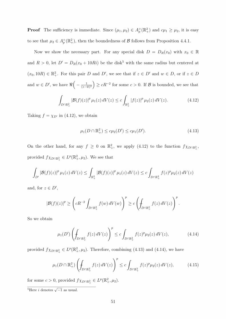
Proof The sufficiency is immediate. Since (µ1, µ2) ∈ A+p (R2

+) and cµ1 ≥ µ2, it is easy

to see that µ2 ∈ A+p (R2

+), then the boundedness of B follows from Proposition 4.4.1.

Now we show the necessary part. For any special disk D = DR(x0) with x0 ∈ R

and R > 0, let D′ = DR(x0 + 10Ri) be the disk5 with the same radius but centered at

(x0, 10R) ∈ R2+. For this pair D and D′, we see that if z ∈ D′ and w ∈ D, or if z ∈ D

and w ∈ D′, we have <(− 1

(z−w)2

)≥ cR−2 for some c > 0. If B is bounded, we see that

∫D∩R2

+

|B(f)(z)|p µ1(z) dV (z) ≤ c

∫R2+

|f(z)|p µ2(z) dV (z). (4.12)

Taking f = χD′ in (4.12), we obtain

µ1(D ∩ R2+) ≤ cµ2(D′) ≤ cµ1(D′). (4.13)

On the other hand, for any f ≥ 0 on R2+, we apply (4.12) to the function fχD∩R2

+,

provided fχD∩R2+∈ Lp(R2

+, µ2). We see that

∫D′|B(f)(z)|p µ1(z) dV (z) ≤

∫R2+

|B(f)(z)|p µ1(z) dV (z) ≤ c

∫D∩R2

+

f(z)pµ2(z) dV (z)

and, for z ∈ D′,

|B(f)(z)|p ≥

(cR−2

∫D∩R2

+

f(w) dV (w)

)p

≥ c

(−∫D∩R2

+

f(z) dV (z)

)p

.

So we obtain

µ1(D′)

(−∫D∩R2

+

f(z) dV (z)

)p

≤ c

∫D∩R2

+

f(z)pµ2(z) dV (z), (4.14)

provided fχD∩R2+∈ Lp(R2

+, µ2). Therefore, combining (4.13) and (4.14), we have

µ1(D ∩ R2+)

(−∫D∩R2

+

f(z) dV (z)

)p

≤ c

∫D∩R2

+

f(z)pµ2(z) dV (z), (4.15)

for some c > 0, provided fχD∩R2+∈ Lp(R2

+, µ2).

5Here i denotes√−1 as usual.

51

To show (4.15) is indeed the A+p (R2

+) condition, we argue as in the proof of the neces-

sary part of [Muc72, Theorem 1]. Suppose that∫D∩R2

+µ2(z)−

p′p dV (z) =∞. Then, by du-

ality of the space Lp(D∩R2+), there is a g ∈ Lp(D∩R2

+), so that∫D∩R2

+g(z)µ2(z)−

1p dV (z) =

∞. Take f = gµ− 1p

2 χD∩R2+

in (4.15). Then∫D∩R2

+f(z) dV (z) =∞ and

∫D∩R2

+f(z)pµ2(z) dV (z) <

∞. So (4.15) gives µ1(D ∩ R2+) = 0, which contradicts the assumption µ1 > 0 almost

everywhere. So we see that∫D∩R2

+µ2(z)−

p′p dV (z) <∞.

Now take f = (µ2)−p′p χD∩R2

+in (4.15) and note that

∫D∩R2

+

f(z)pµ2(z) dV (z) =

∫D∩R2

+

µ2(z)−p′p dV (z) <∞,

since p′

p= p′ − 1. We see (4.15) implies the A+

p (R2+) condition.

In fact, (4.15) is equivalent to the A+p (R2

+) condition. The other direction, the A+p (R2

+)

condition implies (4.15), follows easily from the Holder’s inequality applied to the integral∫D∩R2

+f(z)µ2(z)

1pµ2(z)−

1p dV (z).

52

5. A Wider Class of Weights

In this chapter, we apply Theorem 6 to extend the previous results to a wider class

of weights.

5.1 Alternative Proof of Theorem 2 and Its Extension

Before giving an alternative proof of Theorem 2, we first have the following observa-

tion.

Proposition 5.1.1 For z ∈ R2+, k ∈ Z, s ∈ (0, 2] and p > 1, suppose

µ1(z) =

∣∣∣∣i− zi+ z

∣∣∣∣−(k+1)p+s+2k

and

µ2(z) =

∣∣∣∣i− zi+ z

∣∣∣∣(1−s−k)p+s+2k

,

then (µ1, µ2) /∈ Ap(R2+) for s 6= 2. But we have (µ1, µ2) ∈ A+

p (R2+) if and only if s+ 2k+

2 > (k + 1)p and p(s+ k + 1) > s+ 2k + 2.

Proof To show (µ1, µ2) /∈ Ap(R2+), we consider any disk Dε(i) centered at i with radius

ε < 12. For z ∈ Dε(i), since |i− z| < ε < 1

2, we see that 3

2≤ |i+ z| ≤ 5

2. So, by Definition

4.1.1, we only need to look at

−∫Dε(i)

|i− z|−(k+1)p+s+2k dV (z)

(−∫Dε(i)

|i− z|−p′p

[(1−s−k)p+s+2k] dV (z)

)p/p′.

53

Assuming both integrands are integrable, we obtain ε(s−2)p. But s ∈ (0, 2) and p > 1, so

we see the quantity above tends to ∞ as ε→ 0.

To show (µ1, µ2) ∈ A+p (R2

+), we consider two integrals

I1 =1

|D ∩ R2+|

∫D∩R2

+

∣∣∣∣i− zi+ z

∣∣∣∣−(k+1)p+s+2k

dV (z),

and

I2 =1

|D ∩ R2+|

∫D∩R2

+

∣∣∣∣i− zi+ z

∣∣∣∣− p′p

[(1−s−k)p+s+2k]

dV (z),

where D = DR(x0) is any special disk with radius R centered at x0 ∈ R. Let D0 = D 12(i)

be the disk with radius 12

centered at i. We separate our arguments into two cases.

Case (I), R < 12.

It is easy to see that D ∩ D0 = ∅ hence |i− z| > 12. Note that, as |z| → ∞,∣∣ i−z

i+z

∣∣→ 1, so there is an M such that, when |z| > M , 1 ≥∣∣ i−zi+z

∣∣ ≥ 12. But when |z| ≤M ,

|i+ z| ≤M+1, so 1 ≥∣∣ i−zi+z

∣∣ ≥ 12(M+1)

. Therefore, the integrands in I1 and I2 are bounded

above by some constants that are independent of the special disk D. Then I1Ipp′2 ≤ c, for

some c > 0.

Case (II), R ≥ 12.

We split both I1 and I2 into two integrals respectively, one integrates over D∩R2+\D0

and the other integrates over D ∩ R2+ ∩ D0. For the same reasoning as in case (I), the

parts integrated over D ∩ R2+ \D0 is bounded. The parts integrated over D ∩ R2

+ ∩D0

are bounded respectively by

8

π

∫D0

∣∣∣∣i− zi+ z

∣∣∣∣−(k+1)p+s+2k

dV (z),

and

8

π

∫D0

∣∣∣∣i− zi+ z

∣∣∣∣− p′p

[(1−s−k)p+s+2k]

dV (z).

54

Since |i− z| ≤ 12

for z ∈ D0, we see that 32≤ |i+ z| ≤ 5

2, so the two integrals above are

bounded respectively by

c

∫D0

|i− z|−(k+1)p+s+2k dV (z)

and

c

∫D0

|i− z|−p′p

[(1−s−k)p+s+2k] dV (z).

The first integral above is bounded by a constant if and only if −(k+1)p+s+2k+2 > 0,

and the second is bounded if and only if −p′

p[(1− s− k)p+ s+ 2k] + 2 > 0. Solving the

two inequalities, we see that s+ 2k + 2 > (k + 1)p and p(s+ k + 1) > s+ 2k + 2.

Remark 5.1.2 From the proof we see that if two weights cµ1 ≥ µ2 only have zeros or

poles away from the x-axis and bounded above and below at ∞, then (µ1, µ2) ∈ A+p (R2

+)

if and only if both µ1 and µ− p′p

2 are locally integrable.

Remark 5.1.3 Combining the fact that cµ1 ≥ µ2 with Theorem 6 we see that, for the

Bergman projection on R2+, the two-weight Ap condition is not a necessary condition for

(1.2) (compare to the general Calderon-Zygmund type singular integral). The reason is

that the Bergman kernel is not singular at all on R2+, and it should be a two dimensional

analogue of the so-called Hilbert integral.1

Now we are ready to give an alternative proof of Theorem 2.




, s+2k+2k+1

).


1See also [PS86a,PS86b].

55


p ∈(2− s, 2−s

1−s

).



, s+2k+2s+k+1

).

Proof For s′ = s+ 2k, from (3.1) we know that

Bs′(z, ζ) =s

2(zζ)−(k+1)B0(z, ζ) +

(1− s

2

)(zζ)−kB0(z, ζ)

for z, ζ ∈ D∗. So we may write Bs′ = s2T1 +

(1− s

2

)T2, where T1 is the operator associated

to the kernel (zζ)−(k+1)B0(z, ζ) with weight |ζ|s′

and T2 is the operator associated to the

kernel (zζ)−kB0(z, ζ) with weight |ζ|s′.

For the operator T1, showing its boundedness is the same as showing∫D∗

∣∣∣∣∫D∗

(zζ)−(k+1)f(ζ)

(1− zζ)2|ζ|s

′dV (ζ)

∣∣∣∣p |z|s′ dV (z) ≤ C

∫D∗|f(z)|p |z|s

′dV (z).

By the Cayley transform ϕ : R2+ → D, where ϕ(z) = i−z

i+z, and using the notations in

Chapter 4, we see the above inequality is equivalent to∫R2+−i

∣∣∣∣∣∫R2+−i

− f(w) dV (w)

(z − w)2

∣∣∣∣∣p

µ1(z) dV (z) ≤ C

∫R2+−i

∣∣∣f(z)∣∣∣p µ2(z) dV (z),

where f(z) = f(ϕ(z))ϕ(z)k+1 |ϕ(z)|s−2 · 1(i+1)2

, µ1(z) = 4∣∣ i−zi+z

∣∣−(k+1)p+s+2k ·∣∣∣ 1

(i+z)2

∣∣∣2−p and

µ2(z) = 4∣∣ i−zi+z

∣∣(1−s−k)p+s+2k ·∣∣∣ 1

(i+z)2

∣∣∣2−p. This is exactly (1.2), except that µ1 and µ2 are

only locally integrable on R2+ \ i—not on R2

+. However, since∣∣ i−zi+z

∣∣ ≤ 1 and s ≤ 2,

we have µ1(z)/µ2(z) = |(i− z)/(i+ z)|(s−2)p ≥ 1, so the local integrability of µ2 will be

guaranteed by the local integrability of µ1 at i as we will see below. Moreover, by the

relation µ1 ≥ µ2, Theorem 6 applies,2 that is, T1 is bounded if and only if (µ1, µ2) ∈

A+p (R2

+).

2From the proof of the necessity, we see the boundedness of T1 will imply the local integrability of µ1

and µ2 at i.

56

For the condition (µ1, µ2) ∈ A+p (R2

+), we first note that σ(z) =∣∣∣ 1

(i+z)2

∣∣∣2−p ∈ A+p (R2

+)

for all p > 1. To see this, from the classical result B0 is Lp bounded for all p > 1, where

B0 is the ordinary Bergman projection on D∗ which is the same as the ordinary Bergman

projection on the unit disk. Then (1.2) holds with both µ1 and µ2 replaced by σ, and

hence σ ∈ A+p (R2

+) for all p > 1 by Theorem 6.3

As in Proposition 5.1.1, we consider two integrals

I1 =1

|D ∩ R2+|

∫D∩R2

+

4

∣∣∣∣i− zi+ z

∣∣∣∣−(k+1)p+s+2k

·∣∣∣∣ 1

(i+ z)2

∣∣∣∣2−p dV (z)

and

I2 =1

|D ∩ R2+|

∫D∩R2

+

(4

∣∣∣∣i− zi+ z

∣∣∣∣(1−s−k)p+s+2k

·∣∣∣∣ 1

(i+ z)2

∣∣∣∣2−p)− p′

p

dV (z),

where D = DR(x0) is again any special disk with radius R centered at x0 ∈ R.

For R < 1/2, the same argument as in the proof of Proposition 5.1.1 case (I), shows

that the integrands in I1 and I2 are bounded above by cσ and cσ−p′p respectively. So this

case follows from the fact that σ ∈ A+p (R2

+) for all p > 1.

For R ≥ 1/2, the same argument as in the proof of Proposition 5.1.1 case (II) and

Remark 5.1.2 show that we only need to consider whether

|i− z|−(k+1)p+s+2k and |i− z|−p′p

[(1−s−k)p+s+2k]

are locally integrable away from the x-axis. This shows the local integrabilities of µ1 and

µ2 and, by Proposition 5.1.1, we see this is true if and only if s+ 2k + 2 > (k + 1)p and

p(s+ k + 1) > s+ 2k + 2.

Denoting by U1 = p ∈ (1,∞) | s+ 2k + 2 > (k + 1)p and p(s+ k + 1) > s+ 2k + 2

the range for p, it is not difficult to see that U1 is an open interval. So we obtain

(µ1, µ2) ∈ A+p (R2

+) and hence T1 is bounded if and only if p ∈ U1.

3Indeed, the fact that σ ∈ A+p (R2

+) for all p > 1 can be derived by a direct computation.

57

Similarly, T2 is bounded if and only if (1.2) holds for µ1(z) = 4σ(z)∣∣ i−zi+z

∣∣−kp+s+2k

and µ2(z) = 4σ(z)∣∣ i−zi+z

∣∣−(s+k)p+s+2k. Again, µ1 and µ2 may not be locally integrable.

Fortunately, we have µ1(z)/µ2(z) = |(i− z)/(i+ z)|sp ≤ 1, since |(i− z)(i+ z)| ≤ 1

and s > 0. So we do not need both of µ1 and µ2 to be locally integrable, indeed, they

will not be in some cases. We instead apply Theorem 6 to a single weight, either to

µ1 or to µ2, then by µ1 ≤ µ2 we get the desired inequality. That is, T2 is bounded if

µ1 ∈ A+p (R2

+) ∩ L1loc(R2

+) or µ2 ∈ A+p (R2

+) ∩ L1loc(R2

+).

Following a similar argument, µj ∈ A+p (R2

+) will guarantee the local integrability of

µj, for j = 1, 2. Then we see, by listing all possibilities of k ∈ Z, µ1 ∈ A+p (R2

+) or µ2 ∈

A+p (R2

+) if and only if p ∈ U2 = p ∈ (1,∞) | s+2k+2 > pk and (s+k+2)p > s+2k+2

for s 6= 2. But for s = 2 we do not need to worry about T2, since Bs′ = s2T1 +

(1− s

2

)T2.

It is not hard to see that U2 is also an open interval, and we have T2 is bounded if p ∈ U2.

Now, if both T1 and T2 are bounded, then Bs′ is bounded. Since a simple argument

shows that U1 ⊂ U2 properly, we see that Bs′ is bounded if p ∈ U1. Conversely, if we

look at the endpoint p of U1, then p /∈ U1 but p ∈ U2. In this case, we see that T1 is

unbounded, T2 is bounded, and hence Bs′ is unbounded. So by interpolation we see that

Bs′ is unbounded for all p /∈ U1.

Therefore, for p > 1, Bs′ is bounded if and only if p ∈ U1. When s′ ∈ (0,∞), U1 =(s+2k+2s+k+1

, s+2k+2k+1

). When s′ ∈ [−3, 0], U1 = (1,∞). When s′ ∈ (−4,−3), U1 =

(2−s, 2−s

1−s

).

When s′ = −4, U1 = (1,∞). When s′ ∈ (−∞,−4), U1 =(s+2k+2k+1

, s+2k+2s+k+1

).

Remark 5.1.4 Besides Theorem 6, the analysis for T2 here also supports our Conjecture

1, since the “effective” bound for p is obtained by checking that (µ1, µ2) ∈ A+p (R2

+). Note

that, in this case, we may extend our Conjecture 1 to a more general situation, that is,

without the assumption of local integrabilities of µ1 and µ2.

58

Now we extend the arguments above to prove Theorem 7.

Theorem 7 Assume that p > 1. Let µ(z) = |z|s′|g(z)|2, where g is a non-vanishing

holomorphic function on D and s′ ∈ R. Suppose the weighted Bergman projection B|g|2

on(D, |g|2

)is Lp

(|g|2)

bounded, and suppose the weighted Bergman projection Bs′ on(D∗, |z|s

′ )is Lp

(|z|s

′ )bounded. Then the weighted Bergman projection Bµ on (D∗, µ) is

Lp(µ) bounded.

Moreover, suppose B|g|2 is Lp(|g|2)

bounded if and only if p ∈ (p0, p′0) for some p0 ≥ 1

and suppose Bs′ is Lp(|z|s

′ )bounded if and only if p ∈ (p1, p

′1) for some p1 ≥ 1 as

in Theorem 2. If (p1, p′1) ⊂ (p0, p

′0) properly, then Bµ is Lp(µ) bounded if and only if

p ∈ (p1, p′1).

Proof For the Bergman kernel on the weighted space(D, |g|2

), we have

B|g|2(z, ζ) =1

g(z)g(ζ)

1

(1− zζ)2.

This follows from applying Lemma 2.2.1 with the isometry,

F : L2(D, |g|2

)→ L2(D)

where4 F (f) = fg for f ∈ L2(D, |g|2

). Similar arguments as in the alternative proof

of Theorem 2 show that B|g|2 is Lp bounded if and only if (1.2) holds with both µ1 and

µ2 replaced by σ(z) =∣∣∣g(ϕ(z)) · 1

(i+z)2

∣∣∣2−p. From the statement of Theorem 7, B|g|2 is

Lp(|g|2

)bounded if and only if p ∈ (p0, p

′0) for some p0 ≥ 1. So, by Theorem 6, we see

that σ ∈ A+p (R2

+) if and only if p ∈ (p0, p′0).

Note that µ(z) = |z|s′|g(z)|2 on D∗. The same argument above applies to the weighted

Bergman projection Bµ, whose associated weighted Bergman kernel is

Bµ(z, ζ) =1

g(z)g(ζ)Bs′(z, ζ).

4See also [Zey13, Theorem 3.4].

59

Then by the relation Bs′ = s2T1 +

(1− s

2

)T2 in the alternative proof of Theorem 2 above,

Bµ is Lp(µ) bounded if (1.2) holds both for the first pair

µ1(z) = 4σ(z)

∣∣∣∣i− zi+ z

∣∣∣∣−(k+1)p+s+2k

, µ2(z) = 4σ(z)

∣∣∣∣i− zi+ z

∣∣∣∣(1−s−k)p+s+2k

and for the second pair

µ1(z) = 4σ(z)

∣∣∣∣i− zi+ z

∣∣∣∣−kp+s+2k

, µ2(z) = 4σ(z)

∣∣∣∣i− zi+ z

∣∣∣∣−(s+k)p+s+2k

.

Follow the same argument as in the alternative proof of Theorem 2 above, and noting

that g is bounded above and below on the disk D 12(i) with radius 1

2centered at i, we see

(1.2) holds for the first pair if and only if p ∈ (p0, p′0) ∩ (p1, p

′1). Similarly, (1.2) holds for

the second pair if p ∈ (p0, p′0)∩U , for some larger open interval U which contains p1 and

p′1.5 Therefore Bµ is Lp(µ) bounded if p ∈ (p0, p′0) ∩ (p1, p

′1).

If, in addition, (p1, p′1) ⊂ (p0, p

′0) properly then, for p = p1 and p = p′1, (1.2) fails for

the first pair, but holds for the second. So Bs′,|g|2 is unbounded for these ps. Hence Bµ is

bounded if and only if p ∈ (p1, p′1).

By inflation, we can extend the previous result to a wider class of weights on the

Hartogs triangle. Namely, we consider a weight of the form λ(z) = |z2|s′−2 |g(z2)|2 for

z ∈ H, where g is some non-vanishing holomorphic function on D.

Theorem 8 Assume that p > 1. Let λ be as above, and let p0, p1 be as in Theorem 7.

Then the weighted Bergman projection Bλ on (H, λ) is Lp(λ) bounded if p ∈ (p0, p′0) ∩

(p1, p′1). In addition, if (p1, p

′1) ⊂ (p0, p

′0) properly, then Bλ is Lp(λ) bounded if and only

if p ∈ (p1, p′1).

Proof This is a direct consequence of Proposition 2.2.6 and Theorem 7.

5If (p1, p′1) = (1,∞), then the conclusion is trivial.

60

5.2 A Two-weight Estimate on the Hartogs Triangle

As a last application in this chapter, we use the two-weight inequality to prove the

Lp regularity of the weighted Bergman projection BH,2k+2 on(H, |z2|2k+2 ) mapping from

Lp(H, |z2|2k+2 ) to Lp

(H, |z2|t

)for some t ∈ R. For simplicity, we focus on k ≥ −1 and

k ∈ Z.

Theorem 9 Suppose that BH,2k+2 is the weighted Bergman projection on the weighted

space(H, |z2|2k+2 ). Assume p > 1 and k ≥ −1. Then, for t ≤ 2k + 2, BH,2k+2 is Lp

bounded from Lp(H, |z2|2k+2 ) to Lp

(H, |z2|t

)if and only if p ∈

(2k+6k+4

, t+4k+2

). For t > 2k+2,

BH,2k+2 is bounded from Lp(H, |z2|2k+2 ) to Lp

(H, |z2|t

)if p ∈

(2k+6k+4

, 2k+6k+2

)⋃ (t+4k+4

, t+4k+2

).

Proof The boundedness of the mapping is equivalent to

∫H|BH,2k+2(f)(z)|p |z2|t dV (z) ≤ C

∫H|f(z)|p |z2|2k+2 dV (z).

By Corollary 2.2.2, and considering the biholomorphism Φ : H → D × D∗ via Φ(z) =(z1z2, z2

), the above inequality is equivalent to

∫D×D∗

∣∣∣∣∫D×D∗

B0 ⊗B2k+2(z, ζ)f(ζ) |ζ2|2k+2 dV (ζ)

∣∣∣∣p |z2|t+2−p dV (z)

≤ C

∫D×D∗

|f(z)|p |z2|2k+4−p dV (z),

where B2k+2 is the weighted Bergman kernel on(D∗, |z|2k+2 ) and B0 is the ordinary

Bergman kernel on D. By Lemma 2.2.4, and the fact that the ordinary Bergman pro-

jection on the unit disk is Lp bounded for all p > 1, we see that the above inequality is

equivalent to

∫D∗

∣∣∣∣∫D∗B2k+2(z, ζ)f(ζ) |ζ|2k+2 dV (ζ)

∣∣∣∣p |z|t+2−p dV (z) ≤ C

∫D∗|f(z)|p |z|2k+4−p dV (z).

61

Applying the same argument as in the alternative proof of Theore 2, since s = 2, we see

that BH,2k+2 is bounded if (1.2) holds for

µ1(z) = 4σ(z)

∣∣∣∣i− zi+ z

∣∣∣∣−(k+2)p+t+2

and µ2(z) = 4σ(z)

∣∣∣∣i− zi+ z

∣∣∣∣−(k+2)p+2k+4

,

where σ(z) =∣∣∣ 1

(i+z)2

∣∣∣2−p ∈ A+p (R2

+) for all p > 1.

When t ≤ 2k + 2, Theorem 6 tells us that BH,2k+2 is bounded if and only if p ∈(2k+6k+4

, t+4k+2

). When t > 2k + 2, Theorem 6 again tells us that BH,2k+2 is bounded if

p ∈(

2k+6k+4

, 2k+6k+2

)⋃ (t+4k+4

, t+4k+2

). This completes the proof.

Remark 5.2.1 If we take k = −1 and t = p − 2, then Theorem 9 will imply [CZ14,

Theorem 1.1].

62

6. More Analysis on the A+p (R2

+) Class

To prove Conjecture 1 and Conjecture 2 introduced in Chapter 1, we need a better

understanding of the A+p (R2

+) class. In this chapter, we introduce the special maximal

function operator and prove Theorem 10 and Theorem 11.


In Chapter 4, we introduced the A+p (R2

+) class for p > 1. Now we extend this class to

the case p = 1.

Definition 6.1.1 Two weights µ1 and µ2 on R2+ are in the class A+

1 (R2+), denoted by the

ordered pair (µ1, µ2) ∈ A+1 (R2

+), if there is a c > 0 so that, for all special disks D, we

have

1

|D ∩ R2+|

∫D∩R2

+

µ1(ζ) dV (ζ) ≤ cµ2(z)

for any z ∈ D ∩R2+. For some weight µ, if it satisfies (µ, µ) ∈ A+

1 (R2+), we simply adopt

the notation µ ∈ A+1 (R2

+).

According to the classical results, the Ap class is closely related to the maximal func-

tion operator.1 So it is reasonable to introduce a suitable maximal function operator

associated to the A+p (R2

+) class.

1See [Ste93, Chapter 5] for a general consideration of this topic.

63

Definition 6.1.2 For any measurable function f on R2+, we define the special maximal

function operator M+ by

M+(f)(z) = supz∈D

1

|D ∩ R2+|

∫D∩R2

+

|f(ζ)| dV (ζ)

for z ∈ R2+, where the supremum is taken over all special disks D containing z. It is clear

that M+(f) is lower semi-continuous.

Remark 6.1.1 It is easy to see (µ1, µ2) ∈ A+1 (R2

+) if and only if M+(µ1) ≤ cµ2. In

particular, a weight µ belonging to the class A+1 (R2

+) is equivalent to M+(µ) ≤ cµ.

Remark 6.1.2 It is easy to see, for z, z′ ∈ R2+, that

M+(f)(z′) ≥ M+(f)(z)

whenever <(z′) = <(z) and =(z′) ≤ =(z). Note that the ”absolute value” of the Bergman

projection on the upper half plane

B(f)(z) =

∫R2+

1

|z − w|2f(w) dV (w),

also has the same property above as M+ for f ≥ 0.

Associated to the special maximal function operator M+ and the corresponding special

disks, we also introduce a collection of special squares.

Definition 6.1.3 Let S be the collection of all the special squares of form

Sj,k = x+ iy ∈ R2+ : j · 2k ≤ x ≤ (j + 1) · 2k and 0 ≤ y ≤ 2k,

where j, k ∈ Z. Given a special square Sj,k, we define

S∗j,k = x+ iy ∈ R2+ : (j − 2) · 2k ≤ x ≤ (j + 3) · 2k and 0 ≤ y ≤ 5 · 2k.

64

6.2 Properties of the Special Maximal Function Operator

Before investigating properties of the special maximal function operator, we first give

a simple observation for a special product of two A+1 weights.

Proposition 6.2.1 Suppose that µ1 and µ2 are two weights and µj ∈ A+1 (R2

+), j = 1, 2.

Then, for 1 ≤ p <∞, we have µ1µ1−p2 ∈ A+

p (R2+).

Proof By definition, for j = 1, 2, we have

1

|D ∩ R2+|

∫D∩R2

+

µj(z) dV (z) ≤ c infz∈D∩R2

+

µj(z),

for all special disks D. Then we see that

1

|D ∩ R2+|

∫D∩R2

+

µ1(z)µ2(z)1−p dV (z) ≤ c infz∈D∩R2

+

µ1(z)

(inf

z∈D∩R2+

µ2(z)

)1−p

and(1

|D ∩ R2+|

∫D∩R2

+

(µ1(z)µ2(z)1−p)− p′p dV (z)

) pp′

≤ c

(inf

z∈D∩R2+

µ1(z)

)−1(inf

z∈D∩R2+

µ2(z)

)p−1

.

Combining these two inequalities above, we obtain µ1µ1−p2 ∈ A+

p (R2+).

Remark 6.2.2 From Proposition 6.2.1, we see as long as we have two A+1 (R2

+) weights,

we can construct an A+p (R2

+) weight by taking a special product of the two A+1 (R2

+) weights.

To construct an A+1 (R2

+) weight and consider some mapping properties of M+, we

need two lemmas. The first lemma we introduce is an analogue of [Muc72, Lemma 7].

Lemma 6.2.3 Let f ≥ 0 be an integrable function on R2+, and suppose α > 0. Then

there is a sequence of measurable sets Wl, and a sequence of special squares Sl such

that

(a) The intersection of different Wl’s has measure 0.

65

(b) Sl ⊂ Wl ⊂ S∗l .

(c) α16

∣∣∣Sl∣∣∣ ≤ ∫Wlf(ζ) dV (ζ).

(d) If M+(f)(z) > α, then z ∈ ∪Wl.

Proof Following the idea in [Muc72], we argue as in the classical Calderon-Zygmund

lemma. Since∫R2+f(ζ) dV (ζ) < ∞, there is a k0 ∈ Z+ so that, for all k ≥ k0 and all

j ∈ Z, we have

1

|Sj,k|

∫Sj,k

f(ζ) dV (ζ) ≤ α

16. (6.1)

For the k = k0 − 1 level, to each j ∈ Z, we have either (6.1) still true or

α

16<

1

|Sj,k|

∫Sj,k

f(ζ) dV (ζ) ≤ α

4. (6.2)

The right hand side of (6.2) follows from (6.1) in the k + 1 level. If (6.2) holds for this

j, we collect this special square Sj,k into the sequence Sl, otherwise we continue this

process to the k − 1 level in this Sj,k. Therefore, we obtain a sequence of almost disjoint

special squares Sl satisfying (6.2).

Define W1 = S∗1\(∪m6=1Sm

), and successively let

Wl = S∗l \(∪m 6=lSm

⋃∪l′<lWl′

),

for l > 1. Properties (a) and (b) are easy to check from this definition. Property (c)

follows from Sl ⊂ Wl and Sl satisfies (6.2). If M+(f)(z) > α, then there is a special disk

Dz = Dr(x0) centered at x0 ∈ R with radius r > 0 so that z ∈ Dz and

1

|Dz ∩ R2+|

∫Dz∩R2

+

f(ζ) dV (ζ) > α.

If 2k1−1 ≤ r < 2k1 for some k1 ∈ Z, then Dz intersects at most three special squares Sj,k1 ’s

and it is contained in the union of these squares. Moreover, we have

∣∣Dz ∩ R2+

∣∣ ≤ π

2

∣∣∣Sj,k1∣∣∣ < 4∣∣Dz ∩ R2

+

∣∣ .66

Therefore at least one such special square, say Sj1,k1 , satisfies

∫Dz∩R2

+∩Sj1,k1

f(ζ) dV (ζ) >1

3α∣∣Dz ∩ R2

+

∣∣ .So we obtain ∫

Sj1,k1

f(ζ) dV (ζ) >π

24α∣∣∣Sj1,k1∣∣∣ > α

16

∣∣∣Sj1,k1∣∣∣ .From our construction of the sequence Sl, Sj1,k1 cannot be any of those satisfying (6.1),

so Sj1,k1 is contained in one of the special squares Sl. Since Sj1,k1 intersects Dz, we

must have z ∈ Dz ⊂ S∗j1,k1 ⊂ S∗l1 for some l1. By the definition of Wl, if z is not in

W1, . . . ,Wl1 , then z must be in Sm1 for some m1, hence z ∈ Wm1 , which implies (d).

Lemma 6.2.4 Let f be a measurable funciton on R2+. Then either M+(f)(z) = ∞ for

all z ∈ R2+, or M+(f)(z) <∞ for all z ∈ R2

+.

Proof Assuming that M+(f)(z) = ∞ for some z ∈ R2+, we show that M+(f)(z′) = ∞

for any z′ ∈ R2+. By definition, there is a sequence of special disks Dn with z ∈ Dn and

1

|Dn ∩ R2+|

∫Dn∩R2

+

|f(ζ)| dV (ζ) > n, (6.3)

for all n ∈ Z+. Let rn be the radius of Dn, and let xn be the center, then Dn = Drn(xn).

Since z ∈ Dn, we see rn > =(z) > 0.

If rn is not bounded above then, by selecting a subsequence, we may assume that

lim rn = ∞. Then, given any z′ ∈ R2+, we have rn ≥ |z′ − z| for n sufficiently large. In

this case, it is easy to see z′ ∈ D2rn(xn), the special disk centered at xn with radius 2rn.

From (6.3), we see that

1

|D2rn(xn) ∩ R2+|

∫D2rn (xn)∩R2

+

|f(ζ)| dV (ζ) >1

4n,

for n sufficiently large. This implies M+(f)(z′) =∞.

67

If rn is bounded above then, by selecting a subsequence, we may assume that

lim rn = r, for some r with =(z) ≤ r <∞. Note that, since z ∈ Dn, we have <(z) ∈ Dn,

so Dn ⊂ D3r(<(z)) for n sufficiently large, where D3r(<(z)) is a special disk centered at

<(z) with radius 3r. Therefore, from (6.3), we see that

∫D3r(<(z))∩R2

+

|f(ζ)| dV (ζ) >1

2nπr2

n ≥ cn,

where c = 12π=(z) > 0, for n sufficiently large. So we obtain

∫D3r(<(z))∩R2

+

|f(ζ)| dV (ζ) =∞.

Now, for any z′ ∈ R2+, it is easy to see that z′ ∈ D3r+|z′−z|(<(z)), the special disk centered

at <(z) with radius 3r + |z′ − z|. From the equality above, we have

1∣∣D3r+|z′−z|(<(z)) ∩ R2+

∣∣ ∫D3r+|z′−z|(<(z))∩R2

+

|f(ζ)| dV (ζ) =∞,

which implies M+(f)(z′) =∞. This completes the proof.

Now we are ready to apply M+ to construct A+1 (R2

+) weights.

Theorem 10 Let f be a measurable funciton on R2+. Then, for any 0 < q < 1, the

function(M+(f)

)qis in A+

1 (R2+).

Proof It suffices to show the conclusion for f ≥ 0. By Lemma 6.2.4, we can assume

M+(f)(z) < ∞ for all z ∈ R2+; otherwise, the conclusion is trivial. If M+(f)(z) = 0 for

some z ∈ R2+, then it is easy to see that f = 0 on R2

+. In this case, the conclusiong is

trivial again. So we may assume that 0 < M+(f) <∞ on R2+.

We use an analogue of the argument in [Ste93, Chapter 5.2]. Let µ(z) =(M+(f)(z)

)q;

we show that M+(µ)(z) ≤ cµ(z). That implies µ ∈ A+1 (R2

+).

68

Fixing z ∈ R2+, we normalize f by dividing by M+(f)(z), so we may assume that

M+(f)(z) = 1 and µ(z) = 1. Hence it suffices to show that there is a c > 0 such that

1

|D ∩ R2+|

∫D∩R2

+

µ(ζ) dV (ζ) ≤ c, (6.4)

for any special D containing z.

Given a special disk D = DR(x0) that contains z, let f1 = χD2R(x0)∩R2+f and f2 =

f − f1. We first deal with f1. Let Vα = ζ ∈ D ∩ R2+ : M+(f1)(ζ) > α, we have∫

D∩R2+

(M+(f1)(ζ)

)qdV (ζ) =

∫ ∞0

qαq−1 |Vα| dα

=

∫ 1

0

+

∫ ∞1

qαq−1 |Vα| dα.

(6.5)

Since |Vα| ≤ |D|, we see the first integral of (6.5) is bounded by cR2. For the second

integral, since M+(f)(z) = 1 and z ∈ D2R(x0) ∩ R2+, we see f1 is integrable on R2

+. By

Lemma 6.2.3, we have

|Vα| ≤∑l

∣∣∣S∗l ∣∣∣ =∑l

25∣∣∣Sl∣∣∣

≤ c∑l

1

α

∫Wl

f1(η) dV (η)

≤ c

α

∫R2+

f1(η) dV (η)

=c

α

∫D2R(x0)∩R2

+

f(η) dV (η)

≤ cR2

αM+(f)(z)

=cR2

α.

So the second integral of (6.5) is bounded by cR2. Hence, so is (6.5).

Next we deal with f2. For any ζ ∈ D ∩ R2+, we consider an arbitrary special disk D′r

that contains ζ and whose radius is r. It is easy to see that D′r ⊂ D2r+R(x0). When

69

2r < R, we have D′r ⊂ D2r+R(x0) ⊂ D2R(x0). Since f2 vanishes on D2R(x0) ∩R2+, we see

that

1

|D′r ∩ R2+|

∫D′r∩R2

+

f2(η) dV (η) = 0 < c,

for any c > 0. When 2r ≥ R, then (2r +R)2 ≤ 16r2, so we have∫D′r∩R2

+

f2(η) dV (η) ≤∫D2r+R(x0)∩R2

+

f(η) dV (η)

≤∣∣D2r+R(x0) ∩ R2

+

∣∣ M+(f)(z)

= c(2r +R)2

≤ cr2,

since z ∈ D ⊂ D2r+R(x0). In either case, we obtain

1

|D′r ∩ R2+|

∫D′r∩R2

+

f2(η) dV (η) < c.

Since D′r is arbitrary, we see M+(f2)(ζ) ≤ c, for any ζ ∈ D ∩ R2+. Therefore we obtain∫

D∩R2+

(M+(f2)(ζ)

)qdV (ζ) ≤ cR2. (6.6)

Combining (6.6) with the fact that (6.5) is bounded by cR2, we see that∫D∩R2

+

(M+(f)(ζ)

)qdV (ζ) ≤ cR2,

which implies (6.4). This completes the proof.

Following the idea in [Muc72], we now investigate the weak-type (p, p) mapping prop-

erty of the special maximal function operator M+.

Theorem 11 Assume that p ≥ 1. Suppose µ1 and µ2 are two weights on R2+. Then we

have a weak-type (p, p) inequality: namely, there is a constant c > 0 so that

µ1

(z ∈ R2

+ : M+(f)(z) > α)≤ c

αp

∫R2+

|f(z)|p µ2(z) dV (z) (1.3)

for all α > 0, if and only if (µ1, µ2) ∈ A+p (R2

+).

70

Proof We use an analogue of the argument in [Muc72, Theorem 8]. For the sufficient

part, we only need to prove (1.3) for integrable f ≥ 0. To see this, note that any measur-

able function f ≥ 0 on R2+ can be approximated by the increasing sequence fχDRR>0,

where DR = DR(x0) is a sequence of special disks centered at x0 ∈ R with radius R. Note

that the set z ∈ R2+ : M+(f)(z) > α is the increasing union of the same sets formed

with the fχDR ’s. If we prove (1.3) for fχDR , then the monotonic convergent theorem will

imply (1.3) for f . Note that any fχDR can be approximated by an increasing sequence

of simple functions. Since the support of fχDR is bounded, these simple functions are

integrable. By the same limiting argument, (1.3) for integrable functions will imply (1.3)

for fχDR .

Let Vα = z ∈ R2+ : M+(f)(z) > α. By Lemma 6.2.3, for p > 1, we have

µ1(Vα) ≤∑l

µ1(Wl)

≤∑l

µ1(Wl)

(16

α|Sl|

∫Wl

f(z) dV (z)

)p

≤∑l

c

αpµ1(Wl)

|Sl|

∫Wl

f(z)pµ2(z) dV (z)

(1

|Sl|

∫Wl


)p/p′

≤∑l

c

αp

∫Wl

f(z)pµ2(z) dV (z)µ1(S∗l )

|S∗l |

(1

|S∗l |

∫S∗l


)p/p′

≤∑l

c

αp

∫Wl

f(z)pµ2(z) dV (z)

≤ c

αp

∫R2+

f(z)pµ2(z) dV (z).

71

For p = 1, similarly, we have

µ1(Vα) ≤∑l

16µ1(Wl)

α|Sl|

∫Wl

f(z) dV (z)

≤∑l

c

α

µ1(Wl)

|Sl|

∫Wl

f(z)µ2(z) dV (z)

(infz∈Wl

µ2(z)

)−1

≤∑l

c

α

∫Wl

f(z)µ2(z) dV (z)µ1(S∗l )

|S∗l |

(infz∈S∗l

µ2(z)

)−1

≤ c

α

∫R2+

f(z)µ2(z) dV (z).

For the necessary part, we first consider p > 1. Given any special disk D, we assume

that∫D∩R2

+µ2(z)−

p′p dV (z) = ∞. Then, by duality of the space Lp(D ∩ R2

+), there is a

g ∈ Lp(D∩R2+) so that

∫D∩R2

+g(z)µ2(z)−

1p dV (z) =∞. Let f = gµ

− 1p

2 χD∩R2+

on R2+. Then

M+(f)(z) = ∞ for all z ∈ D ∩ R2+. So (1.3) gives µ1(D ∩ R2

+) = 0, which contradicts

the assumption µ1 > 0 almost everywhere. We also exclude the trivial case µ2 = ∞ on

D ∩ R2+ to see that indeed we have 0 <

∫D∩R2

+µ2(z)−

p′p dV (z) <∞.

Take f = µ− p′p

2 χD∩R2+

and α = 1

|D∩R2+|∫D∩R2

+µ2(z)−

p′p dV (z) in (1.3). We see that

µ1(D ∩ R2+) ≤ c

αp

∫D∩R2

+

µ2(z)−p′µ2(z) dV (z)

=c∣∣D ∩ R2

+

∣∣αp−1

,

which is equivalent to (µ1, µ2) ∈ A+p (R2

+).

When p = 1, given any special disk D, we exclude the trivial case inf µ2 =∞, where

the infimum is taken over all z ∈ D∩R2+. Then, for any ε > 0, there must be a measurable

set U ⊂ D ∩ R2+ with |U | > 0, so that µ2(z) < ε+ inf µ2 on U .

Taking f = χU and α = |U ||D∩R2

+|in (1.3), we see that

µ1(D ∩ R2+) ≤

c∣∣D ∩ R2

+

∣∣|U |

∫U

µ2(z) dV (z)

≤ c∣∣D ∩ R2

+

∣∣(ε+ infz∈D∩R2

+

µ2(z)

).

72

Letting ε → 0+, we see that the inequality above is equivalent to (µ1, µ2) ∈ A+1 (R2

+).


Remark 6.2.5 For any measurable f ≥ 0, we do not have the basic inequality f ≤

M+(f). So we cannot follow the classical approach to show the reverse Holder inequality

for a weight in A+p (R2

+). Hence we cannot obtain the strong-type (p, p) inequality, nor the

factorization of a A+p weight.2

2Compare to the classical results for Ap weights, see [Ste93, Chapter 5] for details.

73

7. Twisted-Weighted Projections


To apply the previous analysis to the twisted-weighted Bergman theory, let us tem-

porarily consider the general setting for a twisted-weighted space. Assume that Ω is a

domain in Cn.

Definition 7.1.1 Suppose τ ∈ C1(Ω) and τ > 0. We define the set of τ -twisted holo-

morphic functions on Ω by

Oτ (Ω) = f ∈ C1(Ω) : ∂τ (f) = 0,

where the τ -twisted ∂τ operator is defined by ∂τ (f) = ∂(τf). Note that Oτ (Ω) is just a

coset of the set of holomorphic functions on Ω, that is, Oτ (Ω) = 1τO(Ω).

Definition 7.1.2 Let µ be a weight on Ω. Define A2τ,µ(Ω) = Oτ (Ω) ∩ L2(Ω, µ). We

say that µ is admissible with respect to τ , if for any compact subset K ⊂ Ω, there is a

constant CK > 0, so that

supK|f(z)| ≤ CK ‖f‖L2(Ω,µ)

for all f ∈ A2τ,µ(Ω). For instance, if µ is continuous and non-vanishing, then it is

admissible.1

1For a more general class of admissible weights, see [McN12, Proposition 2.4] for details.

74

Remark 7.1.1 With an admissible weight µ, A2τ,µ(Ω) is a closed subspace of L2(Ω, µ). To

see this, let fn ⊂ A2τ,µ(Ω) be a sequence that converges to f in L2(Ω, µ). By admissiblity,

for each K ⊂ Ω, fn converges to f uniformly on K. Since τ ∈ C1(Ω), we have supK |τ | ≤

C ′K. Hence τfn converges to τf uniformly on K. Noting that each τfn is holomorphic,

we finally obtain f ∈ Oτ (Ω).

Throughout this chapter, we always assume that the weight µ on the underlying

domain Ω is admissible with respect to the twist factor τ . With this convention, we can

now talk about the orthogonal projection from L2(Ω, µ) to A2τ,µ(Ω).

Definition 7.1.3 Define the twisted-weighted Bergman projection associated to the twist-

weight pair (τ, µ) to be the orthogonal projection Bτ,µ : L2(Ω, µ) → A2τ,µ(Ω), represented

by the integral

Bτ,µ(f)(z) =

∫Ω

Bτ,µ(z, ζ)f(ζ)µ(ζ) dV (ζ),

where Bτ,µ(z, ζ) on Ω× Ω is the twisted-weighted Bergman kernel.

Remark 7.1.2 The twisted-weighted Bergman projection satisfies all the properties of

abstract Bergman theory in a Hilbert space. For example, Bτ,µ is self-adjoint and it

reproduces A2τ,µ(Ω) functions. Note that the twisted-weighted Bergman kernel Bτ,µ(z, ζ)

is ∂τ -closed in the variable z and anti-∂τ -closed in the variable ζ. Moreover, the twisted-

weighted Bergman kernel is uniquely determined by these properties.2

By applying Lemma 2.2.1, we have the following transformation formula, which gen-

eralizes Corollary 2.2.2.

Corollary 7.1.3 Let Φ : Ω1 → Ω2 be a biholomorphism between two domains in Cn.

Suppose that Ωj is equipped with the weight µj and the twist factor τj, j = 1, 2. Assume

2See [McN12, Proposition 2.8] for details.

75

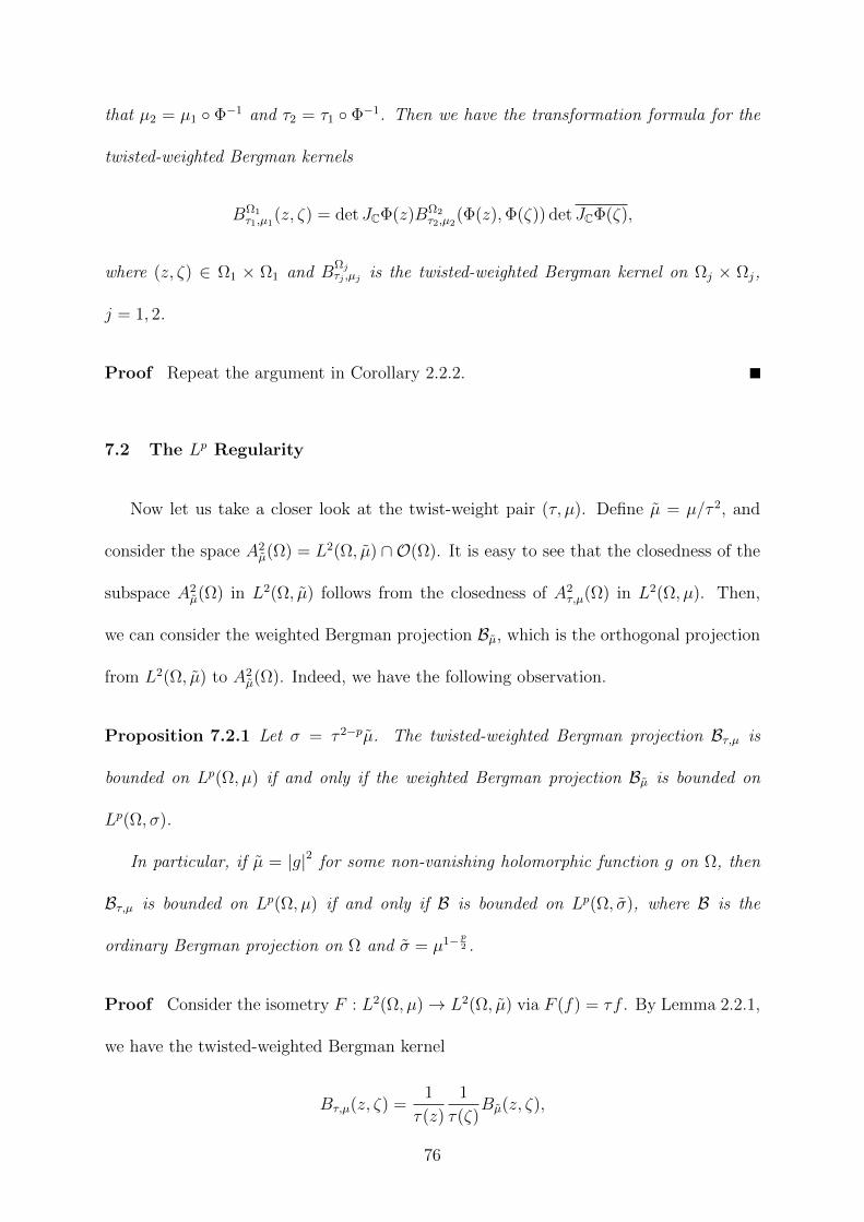
that µ2 = µ1 Φ−1 and τ2 = τ1 Φ−1. Then we have the transformation formula for the

twisted-weighted Bergman kernels

BΩ1τ1,µ1

(z, ζ) = det JCΦ(z)BΩ2τ2,µ2

(Φ(z),Φ(ζ)) det JCΦ(ζ),

where (z, ζ) ∈ Ω1 × Ω1 and BΩjτj ,µj is the twisted-weighted Bergman kernel on Ωj × Ωj,

j = 1, 2.

Proof Repeat the argument in Corollary 2.2.2.

7.2 The Lp Regularity

Now let us take a closer look at the twist-weight pair (τ, µ). Define µ = µ/τ 2, and

consider the space A2µ(Ω) = L2(Ω, µ) ∩ O(Ω). It is easy to see that the closedness of the

subspace A2µ(Ω) in L2(Ω, µ) follows from the closedness of A2

τ,µ(Ω) in L2(Ω, µ). Then,

we can consider the weighted Bergman projection Bµ, which is the orthogonal projection

from L2(Ω, µ) to A2µ(Ω). Indeed, we have the following observation.

Proposition 7.2.1 Let σ = τ 2−pµ. The twisted-weighted Bergman projection Bτ,µ is

bounded on Lp(Ω, µ) if and only if the weighted Bergman projection Bµ is bounded on

Lp(Ω, σ).

In particular, if µ = |g|2 for some non-vanishing holomorphic function g on Ω, then

Bτ,µ is bounded on Lp(Ω, µ) if and only if B is bounded on Lp(Ω, σ), where B is the

ordinary Bergman projection on Ω and σ = µ1− p2 .

Proof Consider the isometry F : L2(Ω, µ)→ L2(Ω, µ) via F (f) = τf . By Lemma 2.2.1,

we have the twisted-weighted Bergman kernel

Bτ,µ(z, ζ) =1

τ(z)

1

τ(ζ)Bµ(z, ζ),

76

where (z, ζ) ∈ Ω×Ω and Bµ is the weighted Bergman kernel on (Ω, µ). By this relation,

we see that

∫Ω

∣∣∣∣∫Ω

Bτ,µ(z, ζ)f(ζ)µ(ζ) dV (ζ)

∣∣∣∣p µ(z) dV (z) ≤ C

∫Ω

|f(z)|p µ(z) dV (z)

is equivalent to

∫Ω

∣∣∣∣∫Ω

Bµ(z, ζ)f(ζ)µ(ζ) dV (ζ)

∣∣∣∣p σ(z) dV (z) ≤ C

∫Ω

∣∣∣f(z)∣∣∣p σ(z) dV (z), (7.1)

where f = τf . This proves the first part of the proposition.

Now we assume that µ = |g|2 for some non-vanishing holomorphic function g on

Ω. Applying Lemma 2.2.1 once again to the isometry F : L2(Ω, |g|2

)→ L2(Ω) via

F (f) = fg, we see that

Bµ(z, ζ) =1

g(z)g(ζ)B(z, ζ),

where (z, ζ) ∈ Ω × Ω and B is the ordinary Bergman kernel on Ω. Hence, (7.1) is

equivalent to

∫Ω

∣∣∣∣∫Ω

B(z, ζ)h(ζ) dV (ζ)

∣∣∣∣p σ(z) dV (z) ≤ C

∫Ω

|h(z)|p σ(z) dV (z), (7.2)

where h = f g. This completes the proof.

Remark 7.2.2 When µ/τ 2 = |g|2, µ is always admissible with respect to τ . An important

observation is that the Lp(Ω, σ) boundedness of B is independent of the choice of τ and

g. Note that, in general, for different τ the coset Oτ is different.

As an application, we now focus on simply connected proper planar domains in C,

and apply Theorem 6 to investigate the Lp regularity of the twisted-weighted Bergman

projection.

77

Theorem 12 Let Ω be a proper simply connected domain in C, and let φ : R2+ → Ω be

a biholomorphism. For a weight µ ∈ C1(Ω) and for any non-vanishing g ∈ O(Ω), define

τ = µ12/ |g|. Then the twisted-weighted Bergman projection Bτ,µ is Lp(Ω, µ) bounded if

and only if µ(φ(z))1− p2 |φ′(z)|2−p ∈ A+

p (R2+).

Proof By Proposition 7.2.1, we see that the twisted-weighted Bergman projection Bτ,µ

is bounded on Lp(Ω, µ) if and only if the ordinary Bergman projection B on Ω is bounded

on Lp(Ω, µ1− p

2

), i.e., (7.2) holds.

Consider the biholomorphism φ : R2+ → Ω. By the transformation formula for ordi-

nary Bergman kernels (a special case of Corollary 2.2.2 or Corollary 7.1.3), we see that

(7.2) is equivalent to

∫R2+

∣∣∣∣∣∫R2+

− f(w)

(z − w)2dV (w)

∣∣∣∣∣p

σ(z) dV (z) ≤ C

∫R2+

|f(z)|p σ(z) dV (z), (7.3)

where σ(z) = |τ(φ(z))g(φ(z))φ′(z)|2−p = µ(φ(z))1− p2 |φ′(z)|2−p. Note that (7.3) is nothing

but (1.2) with both µ1 and µ2 replaced by σ. Therefore, by Theorem 6, we see that (7.3)

holds if and only if σ ∈ A+p (R2

+). This completes the proof.

78

8. The Lp Sobolev Regularity

In this chapter, as the last application, we study the Lp Sobolev mapping property of

the Bergman projection on the Hartogs triangle, and generalize it to higher dimension.


Throughout this chapter, B will denote the Bergman projection on the Hartogs tri-

angle and B will be its associated Bergman kernel, that is,

B(f)(z) =

∫HB(z, ζ)f(ζ) dV (ζ)

for z ∈ H. We then make a precise definition of the weighted Sobolev space on H.

Definition 8.1.1 On the Hartogs triangle H, for each k ∈ Z+ ∪ 0, s ∈ R, and p ∈

(1,∞), we define the weighted Sobolev space by

Lpk(H, |z2|s) = f ∈ L1loc(H) : ‖f‖p,k,s <∞,

where the norm is defined as

‖f‖p,k,s =(∫

H

∑|α|≤k

∣∣Dαz,z(f)(z)

∣∣p |z2|s dV (z)) 1p.

Here α = (α1, α2, α3, α4) is the multi-index running over all |α| ≤ k, and

Dαz,z =

∂|α|

∂zα11 ∂zα2

2 ∂zα31 ∂z

α42

79

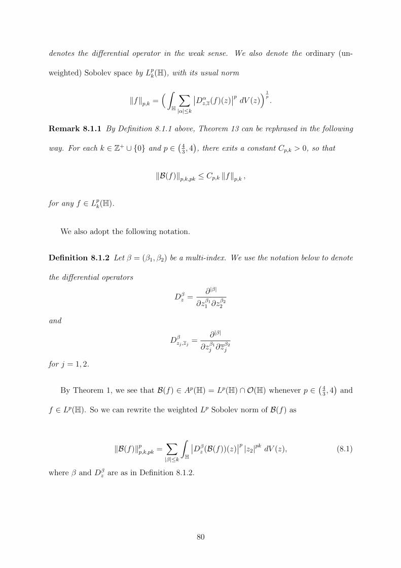
denotes the differential operator in the weak sense. We also denote the ordinary (un-

weighted) Sobolev space by Lpk(H), with its usual norm

‖f‖p,k =(∫

H

∑|α|≤k

∣∣Dαz,z(f)(z)

∣∣p dV (z)) 1p.

Remark 8.1.1 By Definition 8.1.1 above, Theorem 13 can be rephrased in the following

way. For each k ∈ Z+ ∪ 0 and p ∈(

43, 4), there exits a constant Cp,k > 0, so that

‖B(f)‖p,k,pk ≤ Cp,k ‖f‖p,k ,

for any f ∈ Lpk(H).

We also adopt the following notation.

Definition 8.1.2 Let β = (β1, β2) be a multi-index. We use the notation below to denote

the differential operators

Dβz =

∂|β|

∂zβ11 ∂zβ22

and

Dβzj ,zj

=∂|β|

∂zβ1j ∂zβ2j

for j = 1, 2.

By Theorem 1, we see that B(f) ∈ Ap(H) = Lp(H) ∩ O(H) whenever p ∈(

43, 4)

and

f ∈ Lp(H). So we can rewrite the weighted Lp Sobolev norm of B(f) as

‖B(f)‖pp,k,pk =∑|β|≤k

∫H

∣∣Dβz (B(f))(z)

∣∣p |z2|pk dV (z), (8.1)

where β and Dβz are as in Definition 8.1.2.

80

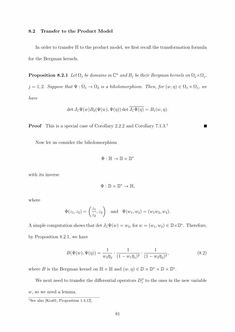
8.2 Transfer to the Product Model

In order to transfer H to the product model, we first recall the transformation formula

for the Bergman kernels.

Proposition 8.2.1 Let Ωj be domains in Cn and Bj be their Bergman kernels on Ωj×Ωj,

j = 1, 2. Suppose that Ψ : Ω1 → Ω2 is a biholomorphism. Then, for (w, η) ∈ Ω1×Ω1, we

have

det JCΨ(w)B2(Ψ(w),Ψ(η)) det JCΨ(η) = B1(w, η).

Proof This is a special case of Corollary 2.2.2 and Corollary 7.1.3.1

Now let us consider the biholomorphism

Φ : H→ D× D∗

with its inverse

Ψ : D× D∗ → H,

where

Φ(z1, z2) =

(z1

z2

, z2

)and Ψ(w1, w2) = (w1w2, w2).

A simple computation shows that det JCΨ(w) = w2, for w = (w1, w2) ∈ D×D∗. Therefore,

by Proposition 8.2.1, we have

B(Ψ(w),Ψ(η)) =1

w2η2

· 1

(1− w1η1)2· 1

(1− w2η2)2, (8.2)

where B is the Bergman kernel on H×H and (w, η) ∈ D× D∗ × D× D∗.

We next need to transfer the differential operators Dβz to the ones in the new variable

w, so we need a lemma.

1See also [Kra01, Proposition 1.4.12].

81

Lemma 8.2.2 Under the above biholomorphism Φ(z) = w, for each β let m = |β|, we

have

Dβz =

∑a+b≤m

pa,b,β(w1)

wm−b2

· ∂a+b

∂wa1∂wb2

, (8.3)

where pa,b,β(w1) is a polynomial of degree at most m in variable w1. In addition, if |β| ≤ k

for some k ∈ Z+ ∪ 0, then |pa,b,β(w1)| ≤ Ck on D uniformly in β, a, and b, for some

constant Ck > 0 depending only on k.

Proof We prove (8.3) by induction on m = |β|. The case m = 0 is trivial. When m = 1,

a direct computation shows that

∂

∂z1

=1

w2

· ∂

∂w1

and

∂

∂z2

= −w1

w2

· ∂

∂w1

+∂

∂w2

.

It is obvious that both of ∂∂z1

and ∂∂z2

are of the form (8.3).

Suppose, for all β with |β| = m, the Dβz ’s are of the form (8.3). We now check the

case |β′| = m + 1. Note that Dβ′z = ∂

∂z1 Dβ

z or Dβ′z = ∂

∂z2 Dβ

z , for some β. By the

inductive assumption, we have

∂

∂z1

Dβz =

1

w2

· ∂

∂w1

∑a+b≤m

pa,b,β(w1)

wm−b2

· ∂a+b

∂wa1∂wb2

=∑

a+b≤m

p′a,b,β(w1)

wm+1−b2

· ∂a+b

∂wa1∂wb2

+pa,b,β(w1)

wm+1−b2

· ∂a+b+1

∂wa+11 ∂wb2

=∑

a+b≤m+1

pa,b,β′(w1)

wm+1−b2

· ∂a+b

∂wa1∂wb2

,

82

and

∂

∂z2

Dβz =

(−w1

w2

· ∂

∂w1

+∂

∂w2

) ∑a+b≤m

pa,b,β(w1)

wm−b2

· ∂a+b

∂wa1∂wb2

=∑

a+b≤m

−w1p′a,b,β(w1)

wm+1−b2

· ∂a+b

∂wa1∂wb2

+−w1pa,b,β(w1)

wm+1−b2

· ∂a+b+1

∂wa+11 ∂wb2

+

(b−m)pa,b,β(w1)

wm+1−b2

· ∂a+b

∂wa1∂wb2

+pa,b,β(w1)

wm−b2

· ∂a+b+1

∂wa1∂wb+12

=∑

a+b≤m+1

pa,b,β′(w1)

wm+1−b2

· ∂a+b

∂wa1∂wb2

.

We see that pa,b,β′(w1) is obviously a polynomial of degree at most m + 1, and Dβ′z has

the form in (8.3).

When |β| ≤ k, all the possible combinations of derivatives in Dβz are finite, so there

are finitely many different coefficients in all of the pa,b,β(w1)’s. Note that |w1| ≤ 1 on D

and a, b ≤ m ≤ k. So we see that |pa,b,β(w1)| ≤ Ck on D as desired.

Now we transfer H to the product model D× D∗ by the biholomorphism Φ, combine

(8.2) and (8.3), and we see the right hand side of (8.1) becomes

∑|β|≤k

∫D×D∗

∣∣∣ ∑a+b≤|β|

∫D×D∗

Ka,b,β(w, η)f(Ψ(η)) |η2|2 dV (η)∣∣∣p |w2|pk+2 dV (w), (8.4)

where

Ka,b,β(w, η) =pa,b,β(w1)

w|β|−b2

· ∂a

∂wa1

( 1

(1− w1η1)2

)· ∂

b

∂wb2

( 1

w2η2

· 1

(1− w2η2)2

).

8.3 Convert the Differential Operators on D∗

Since D∗ is a Reinhardt domain, we can apply a result from [Str86].

Lemma 8.3.1 As in (8.4), for the last factor in Ka,b,β(w, η) we have

∂b

∂wb2

( 1

w2η2

· 1

(1− w2η2)

)=ηb2wb2· ∂

b

∂ηb2

( 1

w2η2

· 1

(1− w2η2)2

). (8.5)

83

Proof By (3.1) in Chapter 3, we see that the kernel in (8.5) is the weighted Bergman

kernel on(D∗, |z|2

). So we can argue step by step as in [Str86, Lemma 2.1] and its

following remark in [Str86, Remark 2.3] to complete the proof.

Now we focus on the integration over D∗ in (8.4). We first define a ”tangential”

operator.

Definition 8.3.1 Let Sw = w ∂∂w

be the complex normal differential operator on a neigh-

borhood of ∂D. We define the tangential operator by

Tw = =(Sw) =1

2i

(w∂

∂w− w ∂

∂w

).

Remark 8.3.2 Indeed, Tw is well-defined on a neighborhood of D. Moreover, for any

disk Dr = |w| < r of radius r < 1 with defining function ρr(w) = |w|2 − r2, we have

Tw(ρr) = 0 (8.6)

on ∂Dr. That is, Tw is tangential on ∂Dr for all r < 1.

In order to make use of integration by parts, we need the following lemma.

Lemma 8.3.3 Let Tw be as above. For b ∈ Z+ ∪ 0, we have

T bw ≡b∑

j=0

cjwj ∂

j

∂wj

(mod

∂

∂w

), (8.7)

where the cjs are constants, cb 6= 0, and T bw denotes the composition of b copies of the

Tws.

Proof We prove (8.7) by induction on b. The case b = 0 is trivial. When b = 1, it is

easy to see that

Tw ≡ −1

2iw∂

∂w

(mod

∂

∂w

).

84

Suppose that (8.7) holds for some b. Then we see that

T bw =b∑

j=0

cjwj ∂

j

∂wj+ A ∂

∂w,

for some operator A. So, for the case b+ 1, we have

Tw T bw =1

2i

(w∂

∂w− w ∂

∂w

)( b∑

j=0

cjwj ∂

j

∂wj+ A ∂

∂w

)

=1

2i

( b∑j=0

cjwwj ∂

j

∂wj∂

∂w− jcjwj

∂j

∂wj− cjwj+1 ∂j+1

∂wj+1

)+ Tw A

∂

∂w

=b+1∑j=0

c′jwj ∂

j

∂wj+ A′ ∂

∂w,

for some constants c′j’s with c′b+1 = − 12icb 6= 0 and some operator A′. Therefore, (8.7)

holds for T b+1w .

Combining (8.5) and (8.7), we note that the kernel in (8.5) is anti-holomorphic in η2.

The inside integration over D∗ with respect to variable η2 in (8.4) denoted by I becomes

I =

∫D∗

∂b

∂wb2

(1

w2η2

· 1

(1− w2η2)2

)f(Ψ(η)) |η2|2 dV (η2)

=

∫D∗

ηb2wb2· ∂

b

∂ηb2

(1

w2η2

· 1

(1− w2η2)2

)f(Ψ(η)) |η2|2 dV (η2)

=1

wb2

∫D∗

b∑j=0

cjTjη2

(1

w2η2

· 1

(1− w2η2)2

)f(Ψ(η)) |η2|2 dV (η2)

=1

wb2

b∑j=0

cj limε→0+

∫D−Dε

T jη2

(1

w2η2

· 1

(1− w2η2)2

)f(Ψ(η)) |η2|2 dV (η2).

Let us assume in addition for a moment that f(Ψ(η)) belongs to C∞(D \ 0) in the

variable η2. Then, by (8.6), we see that

85

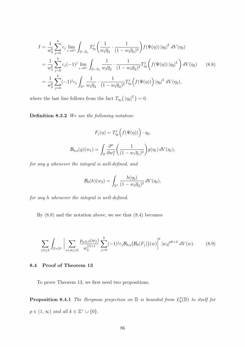
I =1

wb2

b∑j=0

cj limε→0+

∫D−Dε

T jη2

(1

w2η2

· 1

(1− w2η2)2

)f(Ψ(η)) |η2|2 dV (η2)

=1

wb2

b∑j=0

cj(−1)j limε→0+

∫D−Dε

1

w2η2

· 1

(1− w2η2)2T jη2

(f(Ψ(η)) |η2|2

)dV (η2)

=1

wb2

b∑j=0

(−1)jcj

∫D∗

1

w2η2

· 1

(1− w2η2)2T jη2

(f(Ψ(η))

)|η2|2 dV (η2),

(8.8)

where the last line follows from the fact Tη2(|η2|2

)= 0.

Definition 8.3.2 We use the following notation:

Fj(η) = T jη2

(f(Ψ(η))

)· η2,

B0,a(g)(w1) =

∫D

∂a

∂wa1

(1

(1− w1η1)2

)g(η1) dV (η1),

for any g whenever the integral is well-defined, and

B0(h)(w2) =

∫D∗

h(η2)

(1− w2η2)2dV (η2),

for any h whenever the integral is well-defined.

By (8.8) and the notation above, we see that (8.4) becomes

∑|β|≤k

∫D×D∗

∣∣∣∣ ∑a+b≤|β|

pa,b,β(w1)

w|β|+12

b∑j=0

(−1)jcjB0,a

(B0(Fj)

)(w)

∣∣∣∣p |w2|pk+2 dV (w). (8.9)

8.4 Proof of Theorem 13

To prove Theorem 13, we first need two propositions.

Proposition 8.4.1 The Bergman projection on D is bounded from Lpk(D) to itself for

p ∈ (1,∞) and all k ∈ Z+ ∪ 0.

86

Proof This is a special case of the classical result, the regularity of Bergman projec-

tion on bounded smooth domains with strongly pseudoconvex boundary. See [PS77] for

details, or [KR14] for treatment of domains with more general boundary.

Proposition 8.4.2 The integral operator B0, defined as in Definition 8.3.2, is bounded

from Lp(D∗, |w|2−p

)to itself for p ∈

(43, 4), where w ∈ D∗.

Proof This statement is equivalent to the assertion that the weighted Bergman projec-

tion on the weighed space(D∗, |w|2

)is bounded from Lp

(D∗, |w|2

)to itself for p ∈

(43, 4).

See Theorem 2.

Now we are ready to prove Theorem 13 under the additional assumption f(Ψ(η)) ∈

C∞(D \ 0) in the variable η2.

Theorem 13 The Bergman projection BH on the Hartogs triangle H maps continuously

from Lpk(H) to Lpk(H, |z2|pk

)for p ∈

(43, 4).

Proof [Under the additional assumption f(Ψ(η)) ∈ C∞(D \ 0) in the variable η2.]

By (8.1), (8.4), (8.9) and Lemma 8.2.2, we obtain

‖B(f)‖pp,k,pk ≤∑|β|≤k

∑a+b≤|β|

b∑j=0

Cp,k

∫D×D∗

|B0,a(B0(Fj))(w)|p |w2|pk+2−p(|β|+1) dV (w)

≤ Cp,k∑a+b≤k

∫D×D∗

|B0,a(B0(Fb))(w)|p |w2|2−p dV (w).

By Proposition 8.4.1 and Definition 8.3.2, we see that B0,a is bounded from Lpa(D) to

Lp(D). Therefore, for p ∈ (1,∞), we have

87

‖B(f)‖pp,k,pk ≤ Cp,k∑a+b≤k

∫D∗

(∫D

∑|β|≤a

∣∣∣Dβw1,w1

(B0(Fb))(w)∣∣∣p dV (w1)

)|w2|2−p dV (w2)

≤ Cp,k∑|β|+b≤k

∫D

(∫D∗

∣∣∣B0(Dβw1,w1

(Fb))(w)∣∣∣p |w2|2−p dV (w2)

)dV (w1).

Similarly, by Proposition 8.4.2 and Definition 8.3.2, for p ∈(

43, 4)

we have

‖B(f)‖pp,k,pk ≤ Cp,k∑|β|+b≤k

∫D

(∫D∗

∣∣∣Dβw1,w1

(Fb)(w)∣∣∣p |w2|2−p dV (w2)

)dV (w1)

= Cp,k∑|β|+b≤k

∫D×D∗

∣∣∣Dβw1,w1

T bw2

(f(Ψ(w))

)· w2

∣∣∣p |w2|2−p dV (w)

= Cp,k∑|β|+b≤k

∫D×D∗

∣∣∣Dβw1,w1

T bw2

(f(Ψ(w))

)∣∣∣p |w2|2 dV (w)

≤ Cp,k∑

|β|+|β′|≤k

∫D×D∗

∣∣∣Dβw1,w1

Dβ′

w2,w2

(f(Ψ(w))

)∣∣∣p |w2|2 dV (w),

(8.10)

where the last line follows from Tw2 = 12i

(w2

∂∂w2− w2

∂∂w2

), |w2| < 1 for w2 ∈ D∗, and an

equation similar to (8.7).

Note that, under the biholomorphism Ψ(w) = z defined in §8.2, we have

∂

∂w1

= w2∂

∂z1

and∂

∂w1

= w2∂

∂z1

,

and also

∂

∂w2

= w1∂

∂z1

+∂

∂z2

and∂

∂w2

= w1∂

∂z1

+∂

∂z2

.

Again, since (w1, w2) ∈ D× D∗, we see that |w1| , |w2| < 1. Therefore, by (8.10) and the

transfer of D× D∗ back to H, we finally arrive at

‖B(f)‖pp,k,pk ≤ Cp,k∑|α|≤k

∫H

∣∣Dαz,z(f)(z)

∣∣p dV (z)

as desired.

88

To remove the additional assumption f(Ψ(η)) ∈ C∞(D \ 0) in variable η2, we need

the following lemma.

Lemma 8.4.3 The subspace C∞(D \ 0)⋂Lpk(D∗, |w|2

)is dense in Lpk

(D∗, |w|2

)with

respect to the weighted norm in Lpk(D∗, |w|2

).

Proof The argument is based on the ideas from [Eva98, §5.3 Theorem 2 and Theorem

3].

Given any g ∈ Lpk(D∗, |w|2

), we fix a δ > 0. On V0 = D \ D 1

2, the weighted norm

Lpk(V0, |w|2

)is equivalent to the unweighted norm Lpk(V0). Arguing as in the proof of

[Eva98, §5.3 Theorem 3], we see that there is a g0 ∈ C∞(V0), so that

‖g0 − g‖Lpk(V0,|w|2) < δ.

Define Uj = Dρ− 1j\D 1

jfor some 1 > ρ > 1

2and for j ∈ Z+ (U1 = ∅). Let Vj = Uj+3\Uj+1.

Then we see that⋃∞j=1 Vj = Dρ \ 0. Arguing as in the proof of [Eva98, §5.3 Theorem

2], we can find a smooth partition of unity ψj∞j=1 subordinate to Vj∞j=1, so that∑∞j=1 ψj = 1 on Dρ\0. Moreover, for each j, the support of ψjg lies in Vj

(so |w| > 1

j+3

),

and hence ψjg ∈ Lpk(Dρ \ 0). Therefore we can find smooth function gj, with support

in Uj+4 \ Uj, so that

‖gj − ψjg‖Lpk(Dρ\0) ≤δ

2j,

see [Eva98, §5.3 Theorem 2] for details. Write g0 =∑∞

j=1 gj. It is easy to see that

g0 ∈ C∞(Dρ \ 0) and

‖g0 − g‖Lpk(Dρ\0,|w|2) ≤ ‖g0 − g‖Lpk(Dρ\0) ≤ δ,

since |w| < 1 on Dρ \ 0.

89

Let V ′0 be an open set so that ∂D ⊂ V ′0 and V ′0⋂

D = V0. Then V ′0⋃Dρ cover D. Take

a smooth partition of unity ψ1, ψ2 on D subordinate to V ′0 ,Dρ. Then h = ψ1g0 + ψ2g0

belongs to C∞(D \ 0), and

‖h− g‖Lpk(D∗,|w|2) ≤ C(‖g0 − g‖Lpk(V0,|w|2) + ‖g0 − g‖Lpk(Dρ\0,|w|2)

)< 2Cδ

as desired.

Now we are ready to remove the extra assumption and prove Theorem 13.

Proof of Theorem 13:

For any f ∈ Lpk(H), we have f(Ψ(w)) ∈ Lpk(D∗, |w2|2

)in the variable w2. Then, by

Lemma 8.4.3, we can find a sequence hj(w) ⊂ C∞(D \ 0) tending to f(Ψ(w)) in the

variable w2 with respect to the norm in Lpk(D∗, |w2|2

). We have already seen that (8.10)

holds for each hj(w) replacing f(Ψ(w)). Indeed, if we focus on the integration over D∗,

by comparing with (8.4), we see that (8.10) is just the following. For each b = 0, 1, . . . , k,

∫D∗

∣∣∣∣wb2 ∂b

∂wb2(B2(hj))

∣∣∣∣p |w2|2 dV (w2) ≤ Cp,k ‖hj‖Lpk(D∗,|w2|2) , (8.11)

where B2 is the weighted Bergman projection on the weighted space(D∗, |w2|2

).

Now let j → ∞. In view of the boundedness of B2 (by Theorem 2 (a)), we see that

wb2∂b

∂wb2(B2(hj)) indeed tends to wb2

∂b

∂wb2(B2(f(Ψ))) in Lp

(D∗, |w2|2

)for each b = 0, 1, . . . , k.

Therefore (8.11) is valid for general f(Ψ(w)) ∈ Lpk(D∗, |w2|2

), which completes the proof

for general f ∈ Lpk(H).

Remark 8.4.4 If we consider a general weighted space Lpk(H, |z2|s) rather than Lpk(H, |z2|pk

),

we can use the same idea and apply the two-weight inequality in Chapter 4 to derive the

boundedness of B for p ∈(

43, s+4k+1

)and s ≤ pk. When s = 0 and k = 1, we see that we

90

cannot derive the boundedness even for p = 2. This coincides with the fact that B is not

bounded from W 1(H) to itself for the unweighted case, see [CS13].2

Remark 8.4.5 We may also consider the weighted Sobolev space with weights inhomo-

geneous with respect to derivatives of different orders.

To be precise, for each k ∈ Z+ ∪ 0, p ∈ (1,∞), and t = tm∞m=0 ∈ Rω, we define

the inhomogeneous weighted Sobolev space by

Lpk(|z2|t

)= f ∈ L1

loc(H) : ‖f‖p,k,t <∞,

where the norm is defined as

‖f‖p,k,t =(∫

H

∑|α|≤k

∣∣Dαz,z(f)(z)

∣∣p |z2|t|α| dz) 1p.

Then a variant of Theorem 13 can be stated as follows. (The proof is almost the same.)

For each k ∈ Z+ ∪ 0 and p ∈(

43, 4), suppose that t = tm∞m=0 ∈ Rω and tm = mp.

Then there exits a constant Cp,k > 0 so that

‖B(f)‖p,k,t ≤ Cp,k ‖f‖p,k

for any f ∈ Lpk(H).

8.5 Generalization to n-dimensional Hartogs Triangle

The method also applies to the n-dimensional Hartogs triangle. Using the notation

in (1.1), we have the following result.

Theorem 14 The Bergman projection on the n-dimensional Hartogs triangle Hnφj

maps

continuously from Lpk(Hnφj

)to Lpk

(Hnφj, |z′′1 |

pk ) for p ∈(

2nn+1

, 2nn−1

).

2See also [Zey13] for variants of Hartogs triangle.

91

The idea of the proof remains the same, but requires more complicated computations.

We outline it very briefly here.

Proof Using the same argument as in the proof of Theorem 5 in Chapter 3, it suffices

to prove the theorem for the domain

Hn = (z′, z′′) ∈ Cm1+···+ml+d : max1≤j≤l

|zj| < |z′′1 | < |z′′2 | < · · · < |z′′d | < 1.

As in §8.2, we transfer Hn to a product model by Φ : Hn → Bm1×· · ·×Bml×(D∗)×d

,

with

Φ(z′, z′′) =

(z′

z′′1,z′′1z′′2, . . . ,

z′′d−1

z′′d, z′′d

)= (w′, w′′1 , . . . , w

′′d).

By induction, (8.3) becomes

Dβz =

∑|a|+|b|≤|β|

pa,b,β(w)

w′′b· ∂|a|+|b|

∂w′a∂w′′b, (8.12)

where β is an n-dimensional multi-index, a is m-dimensional, and both b and b are d-

dimensional with bj + bj ≤ |β| for j = 1, . . . , d− 1 and bd + bd = |β|.

While converting the differential operators on D∗, (8.5) applies to the weighted Bergman

kernel on the weighted space(D∗, |w|2(j−1) ), for j = n− d+ 1, n− d+ 2, . . . , n. By using

(8.5), (8.6), (8.7), and integration by parts, we arrive at a similar expression as (8.9).

Classical result tells us that, for j = 1, . . . , l, the Lpk boundedness of the Bergman

projection on Bmj holds for p ∈ (1,∞). Thus we only need to take care of the Lp

boundedness of the weighted Bergman projection on(D∗, |w|2(j−1) ), for j = n−d+1, n−

d+ 2, . . . , n. By Theorem 2, all these projections will be bounded when p ∈(

2nn+1

, 2nn−1

).

The proof will be complete once we pass from C∞(D \ 0) to Lpk(D∗, |w|2(j−1) ) for

j = n− d+ 1, n− d+ 2, . . . , n, by applying a general version of Lemma 8.4.3.

92

Remark 8.5.1 The reason we consider the weight |z′′1 |pk rather than |z′′d |

pk is that, if we

look at (8.12) and apply (8.5), then we will obtain a factor 1

|w′′j |bj+bjwith bj + bj ≤ |β| ≤ k

for j = 1, . . . , d. For each j, the equality will hold in some cases. Therefore, for each j,

it is required to consider a weight∣∣w′′j ∣∣pk to cancel out with the factor. By transferring

the product model back to Hn, we obtain a weight |z′′1 |pk.

93

REFERENCES

[Bar84] D. Barrett, Irregularity of the Bergman projection on a smooth bounded

domain in C2, Ann. of Math. 119 no. 2 (1984), 431–436.

[Bar92] D. Barrett, Behavior of the Bergman projection on the Diederich-Fornæss

worm, Acta Math 168 (1992), 1–10.

[Bel81] S. Bell, Biholomorphic mappings and the ∂-problem, Ann. of Math. 114

(1981), 103–113.

[BS12] D. Barrett and S. Sahutoglu, Irregularity of the Bergman projection on worm

domains in Cn, Michigan Math. J. 61 no. 1 (2012), 187–198.

[CD06] P. Charpentier and Y. Dupain, Estimates for the Bergman and Szego Projec-

tions for pseudoconvex domains of finite type with locally diagonalizable Levi

forms, Publ. Mat. 50 (2006), 413–446.

[Chr96] M. Christ, Global C∞ irregularity of the ∂-Neumann problem for worm do-

mains, J. Amer. Math. Soc. 9 (1996), 1171–1185.

[CS11] D. Chakrabarti and M.-C. Shaw, The Cauchy-Riemann equations on product

domains, Math. Ann. 349 no. 4 (2011), 977–998.

[CS13] D. Chakrabarti and M.-C. Shaw, Sobolev regularity of the ∂-equation on the

Hartogs triangle, Math. Ann. 356 no. 1 (2013), 241–258.

94

[CZ14] D. Chakrabarti and Y. E. Zeytuncu, Lp mapping properties of the Bergman

projection on the Hartogs triangle, arXiv:1410.1105 [math.CV] (Oct. 2014).

[Eva98] L. C. Evans, Partial Differential Equations, Amer. Math. Soc., Providence,

RI, 1998. Fourth printing, 2008.

[Fef74] C. Fefferman, The Bergman kernel and biholomorphic mappings of pseudo-

convex domains, Invent. Math. 26 (1974), 1–65.

[HKZ00] H. Hedenmalm, B. Korenblum and K. Zhu, Theory of Bergman spaces,

Springer-Verlag, Berlin, Heidelberg, New York, 2000.

[KP07] S. Krantz and M. Peloso, New results on the Bergman kernel of the worm

domain in complex space, Electron. Res. Announc. Math. Sci. 14 (2007),

35–41.

[KP08] S. Krantz and M. Peloso, The Bergman kernel and projection on non-smooth

worm domains, Houston J. Math. 34 (2008), 873–950.

[KR14] T. Khanh and A. Raich, Local regularity properties for the Bergman pro-

jection on pseudoconvex domains of finite/infinite type, arXiv:1406.6532

[math.CV] (Jun. 2014).

[Kra01] S. Krantz, Function theory of several complex variables, 2nd ed., Amer. Math.

Soc., Providence, RI, 2001.

[Kra13] S. Krantz, Geometric analysis of the Bergman kernel and metric, Springer,

2013.

[LS04] L. Lanzani and E. M. Stein, Szego and Bergman projections on non-smooth

planar domains, J. Geom. Anal. 14 no. 1 (2004), 63–86.

95

[LS12] L. Lanzani and E. M. Stein, The Bergman projection in Lp for domains with

minimal smoothness, Illinois J. Math. 56 no. 1 (2012), 127–154.

[McN89] J. McNeal, Boundary behavior of the Bergman kernel function in C2, Duke

Math. J. 58 no. 2 (1989), 499–512.

[McN94] J. McNeal, Estimates on the Bergman kernel of convex domains, Adv. in

Math. 109 (1994), 108–139.

[McN12] J. McNeal, Non-holomorphic projections and extension of biholomorphic map-

pings, arXiv:1205.0284 [math.CV] (May 2012).

[MS94] J. McNeal and E. M. Stein, Mapping properties of the Bergman projection

on convex domains of finite type, Duke Math. J. 73 no. 1 (1994), 177–199.

[Muc72] B. Muckenhoupt, Weighted norm inequalities for the Hardy maximal function,

Trans. Amer. Math. Soc. 165 (Mar.,1972), 207–226.

[Neu83] C. J. Neugebauer, Inserting Ap-weights, Proc. Amer. Math. Soc. 87 no. 4

(1983), 644–648.

[NRSW89] A. Nagel, J.-P. Rosay, E. M. Stein and S. Wainger, Estimates for the Bergman

and Szego kernels in C2, Ann. of Math. 129 no. 2 (1989), 113–149.

[PS77] D. Phong and E. M. Stein, Estimates for the Bergman and Szego projections

on strongly pseudoconvex domains, Duke Math. J. 44 no. 3 (1977), 695–704.

[PS86a] D. Phong and E. M. Stein, Hilbert integrals, singular integrals, and Radon

transforms I, Acta Math. 157 no. 1 (1986), 99–157.

[PS86b] D. Phong and E. M. Stein, Hilbert integrals, singular integrals, and Radon

transforms II, Invent. math. 86 (1986), 75–113.

96

[Rud80] W. Rudin, Function theory in the unit ball of Cn, Springer-Verlag, Berlin,

Heidelberg, New York, 1980.

[Ste93] E. M. Stein, Harmonic Analysis: Real-Variable Methods, Orthogonality, and

Oscillatory Integrals, Princeton Univ. Press, 1993. Second printing, 1995.

[Str86] E. Straube, Exact regularity of Bergman, Szego and Sobolev space projections

in non-pseudoconvex domains, Math. Z. 192 (1986), 117–128.

[Str10] E. Straube, Lectures on the L2-Sobolev Theory of the ∂-Neumann Problem,

ESI Lectures in Mathematics and Physics, European Mathematical Society

(EMS), Zurich, 2010.

[Zey13] Y. E. Zeytuncu, Lp regularity of weighted Bergman projections, Trans. Amer.

Math. Soc. 365 no. 6 (2013), 2959–2976.

97

Documents

Regularity of the Bergman Projection on Variants of the