Lecture 12: Robust regression

http://polisci.msu.edu/icpsr/regress3

Regression III:Advanced Methods

Bill JacobyMichigan State University

2

Goals of the lecture

• Introduce the idea of “robustness”, in particular, distributional robustness

• Discuss robust and resistant regressionmethods that can be used when there are unusual observations or skewed distributions

• Particular emphasis will be placed on:– M-Estimation– Bounded-Influence Regression

3

Defining “Robust” (1)• Following Huber (1981) we will interpret robustness

as insensitivity to small deviations from the assumptions the model imposes on the data.

• In particular, we are interested in distributional robustness, and the impact of skewed distributions and/or outliers on regression estimates.– In this context, “robust” refers to the shape of a

distribution (specifically, when it differs from the theoretically assumed distribution

– Although conceptually distinct, distributional robustness and outlier resistance are, for practical purposes, synonymous

– Robust can also be used to describe standard errors that are adjusted for non-constant error variance (This is a different topic!!! We will discuss later …)

4

Defining “Robust” (2)

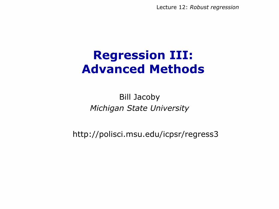
• Statistical inferences are based both on observations and on prior assumptions about underlying distributions and relationships between variables

• Although these assumptions are never exactly true, some statistical models are more sensitive to small deviations from these assumptions than others

• A model is robust if it has the following features:– Reasonably efficient and unbiased– Small deviations from the model assumptions will not

substantially impair the performance of the model– Somewhat larger deviations will not invalidate the

model completely

5

Influential Cases and OLS

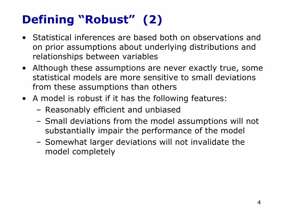
• OLS is not robust to outliers. It can produce misleading results if unusual cases go undetected—even a single case can have a significant impact on the fit of the regression surface

• Moreover, the efficiency of the OLS regression can be hindered by heavy-tailed distributions and outliers

• Diagnostics can be used to detect non-normal error distributions and influential cases. But, once they are found, what should we do?

• Investigate whether the deviations are a symptom of model failure that can be repaired by deleting cases, transformations, or adding more terms to the model– In cases when the unusual cases cannot be remedied

this way,, robust regression can provide an alternative to OLS

– Robust regression can also be used as a diagnostic tool

6

Inequality model revisited (1)

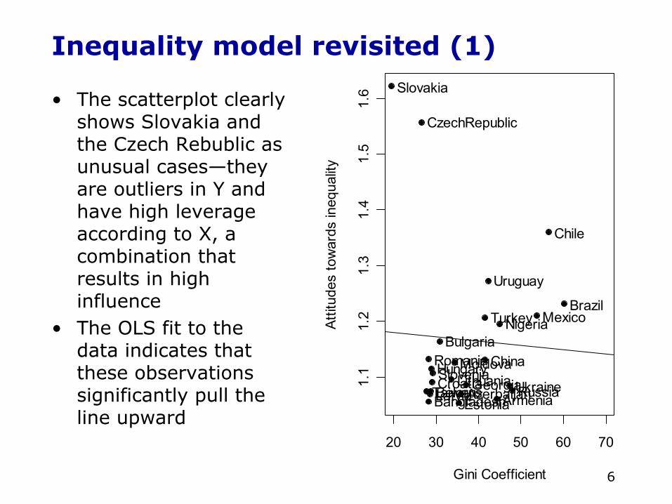
• The scatterplot clearly shows Slovakia and the Czech Rebublic as unusual cases—they are outliers in Y and have high leverage according to X, a combination that results in high influence

• The OLS fit to the data indicates that these observations significantly pull the line upward

20 30 40 50 60 70

1.1

1.2

1.3

1.4

1.5

1.6

Gini Coefficient

Attit

udes

tow

ards

ineq

ualit

yMexico

Hungary

BrazilNigeria

Chile

Belarus

CzechRepublic

Slovenia

BulgariaRomania China

Taiwan

Turkey

LithuaniaLatviaEstonia

UkraineRussia

Uruguay

MoldovaGeorgia

ArmeniaAzerbaijanBangladeshCroatia

Slovakia

7

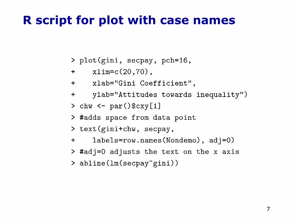
R script for plot with case names

8

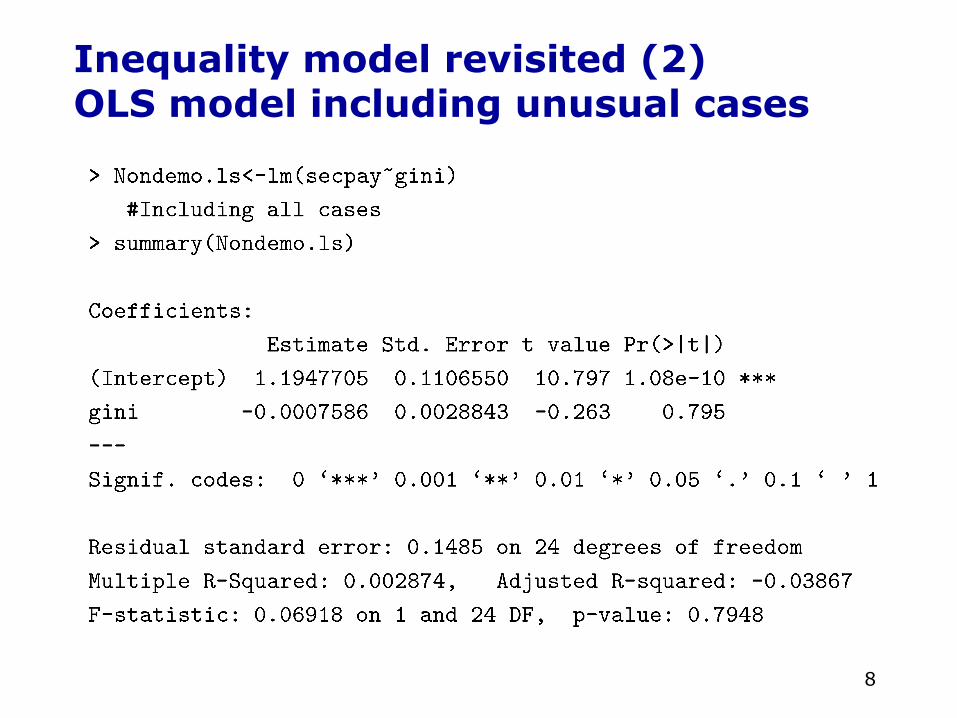
Inequality model revisited (2)OLS model including unusual cases

9

Inequality model revisited (3)Diagnostics• Given the poor fit of OLS model, we now proceed to do

some further diagnostics• In particular, we examine the quantile comparison plot,

checking for a skewed distribution• We also look at the Cook’s D to explore the impact of

individual cases on the regression line (using an influence plot)

• Recall that, if this were a multiple regression model, we would also explore the partial-regression plots—added-variable plots—for influence)

10

Inequality model revisited (4)Outlier Tests

-2 -1 0 1 2

-10

12

34

Studentized residuals for Inequality model

t Quantiles

Stud

entiz

ed R

esid

uals

(Non

dem

o.ls

)

24 16

7

26

11

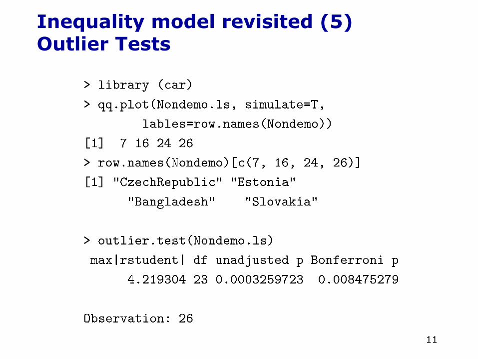
Inequality model revisited (5)Outlier Tests

12

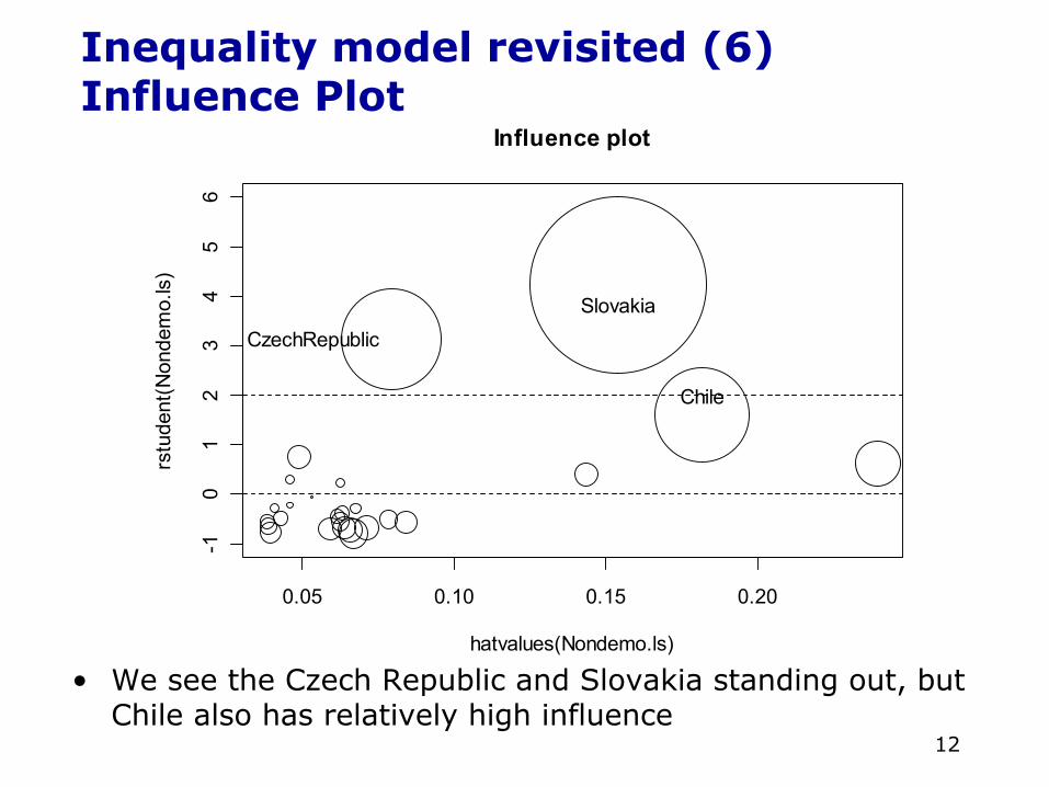
Inequality model revisited (6)Influence Plot

• We see the Czech Republic and Slovakia standing out, but Chile also has relatively high influence

0.05 0.10 0.15 0.20

-10

12

34

56

Influence plot

hatvalues(Nondemo.ls)

rstu

dent

(Non

dem

o.ls

)

Chile

CzechRepublicSlovakia

13

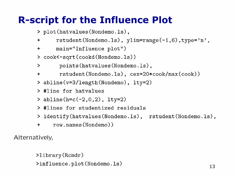
R-script for the Influence Plot

14

Inequality model revisited (7)OLS model without influential cases

• We now proceed to explore various robust regression methods to see how their results compare

15

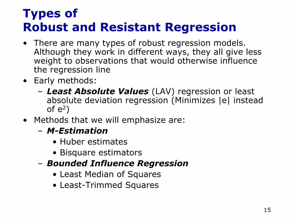
Types of Robust and Resistant Regression• There are many types of robust regression models.

Although they work in different ways, they all give less weight to observations that would otherwise influence the regression line

• Early methods:– Least Absolute Values (LAV) regression or least

absolute deviation regression (Minimizes |e| instead of e2)

• Methods that we will emphasize are:– M-Estimation

• Huber estimates• Bisquare estimators

– Bounded Influence Regression• Least Median of Squares• Least-Trimmed Squares

16

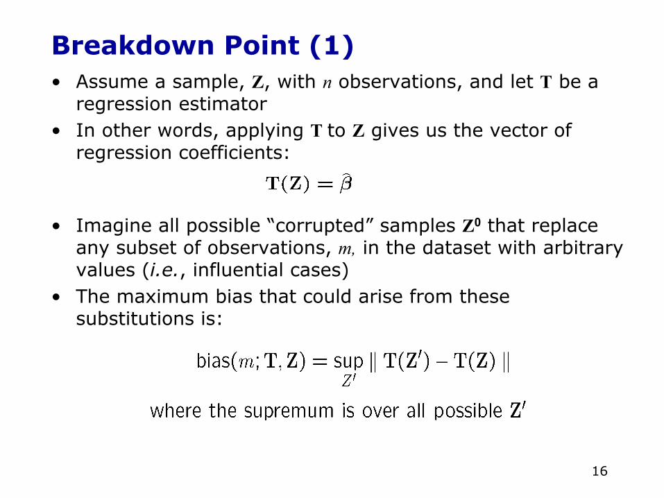
Breakdown Point (1)• Assume a sample, Z, with n observations, and let T be a

regression estimator• In other words, applying T to Z gives us the vector of

regression coefficients:

• Imagine all possible “corrupted” samples Z0 that replace any subset of observations, m, in the dataset with arbitrary values (i.e., influential cases)

• The maximum bias that could arise from these substitutions is:

17

Breakdown Point (2)

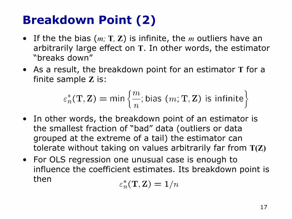
• If the the bias (m; T, Z) is infinite, the m outliers have an arbitrarily large effect on T. In other words, the estimator “breaks down”

• As a result, the breakdown point for an estimator T for a finite sample Z is:

• In other words, the breakdown point of an estimator is the smallest fraction of “bad” data (outliers or data grouped at the extreme of a tail) the estimator can tolerate without taking on values arbitrarily far from T(Z)

• For OLS regression one unusual case is enough to influence the coefficient estimates. Its breakdown point is then

18

Breakdown Point (3)• As n gets larger, 1/n tends towards 0, meaning that the

breakdown point for OLS is 0%• Robust and resistant regression methods attempt to limit

the impact of unusual cases on the regression estimates– Least Absolute Values (LAV) regression is robust to

outliers (unusual Y values given X), but typically fares even worse than OLS for cases with high leverage• If a leverage point is very far away, the LAV line will

pass through it. In other words, its breakdown point is also 1/n

– More efficient than LAV estimators, M-Estimators are also robust to outliers but can have trouble handling cases with high leverage, meaning that the breakdown point is also 1/n

– Bounded influence methods have a much higher breakdown point (as high as 50%) because they effectively remove a large proportion of the cases. These methods can have trouble with small samples, however

19

Estimating the Centre of a Distribution• In order to explain how robust regression works it is

helpful to start with the simple case of robust estimation of the centre of a distribution

• Consider independent observations and the simple model:

• If the underlying distribution is normal, the sample mean is the maximally efficient estimator of µ, producing the fitted model:

• The mean then minimizes the least-squares objective function:

20

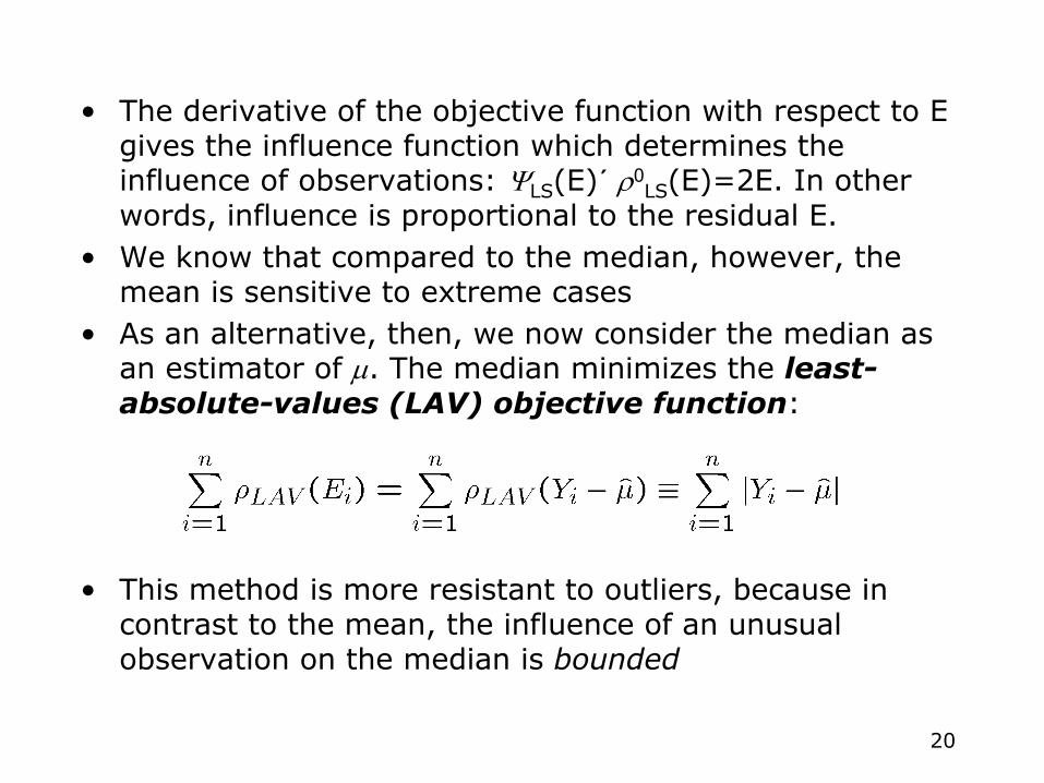
• The derivative of the objective function with respect to E gives the influence function which determines the influence of observations: ΨLS(E)´ ρ0

LS(E)=2E. In other words, influence is proportional to the residual E.

• We know that compared to the median, however, the mean is sensitive to extreme cases

• As an alternative, then, we now consider the median as an estimator of µ. The median minimizes the least-absolute-values (LAV) objective function:

• This method is more resistant to outliers, because in contrast to the mean, the influence of an unusual observation on the median is bounded

21

• Again taking the derivative of the objective function gives the shape of the influence function:

• The fact that the median is more resistant than the mean to outliers is a favourable characteristic.

• It is far less efficient, however. If Y~N(µ,σ2), the sampling variance is σ2/n; the variance for the median is πσ2/2n– In other words the sampling variance for the median

is π/2 ' 1.57 times as large as for the mean• LAV regression, then, simply minimizes ∑ |Ei| where the

absolute residuals are based on the median

22

Influence Functions for the Mean (a) and Median (b)

23

LAV Regression in R (1)

• The LAV model is very resistant here because the influence is largely due to high Y-values—The slope for Gini is nearly the same as the OLS model excluding the Czech Republic and Slovakia

24

LAV Regression in R (2)

• A plot of the residuals from the LAV regression shows that Slovakia and the Czech Republic are far from the fitted line, indicating that they would be influential in a regular OLS regression

0 5 10 15 20 25-0

.10.

00.

10.

20.

30.

40.

5

Index

resi

dual

s(N

onde

mo.

lav)

CzechRepublic

Slovakia

25

M-Estimation: Huber Estimates (1)

• A good compromise between the efficiency of the least-squares and the robustness of the least-absolute values estimators is the Huber objective function

• At the centre of the distribution the Huber function behaves like the OLS function, but at the extremes it behaves like the LAV function:

• The influence function is determined by taking the derivative:

• The tuning constant, k, defines the centre and tails

26

M-Estimation: Huber weightsk, the tuning constant• The tuning constant is expressed as a multiple of the

scale (the spread) of Y, k=cS, where S is the measure of the scale of Y (i.e., the spread)– We could use the standard deviation as a measure of

scale, but it is more influenced by extreme observations than is the mean

– Instead, we use the median absolute deviation:

• The median of Y serves as an initial estimate of µ-hat, thus allowing us to define S´ MAD/.6745, which ensures that S estimates σ when the population is normal

• Using k=1.345 (1.345/.6745 is about 2) produces 95% efficiency relative to the sample mean when the population is normal and gives substantial resistance to outliers when it is not

• A smaller k gives more resistance

27

M-Estimation: Biweight Estimates

• Biweight estimates behave somewhat differently than Huber weights, but are calculated in a similar manner

• The biweight objective function is especially resistant to observations on the extreme tails:

• The influence function, then, tends toward zero:

• For this function a tuning constant of k=4.685/.6745, or about 7 MADS, produces 95% efficiency when sampling from a normal population

28

Weight Functions for Various Estimators

29

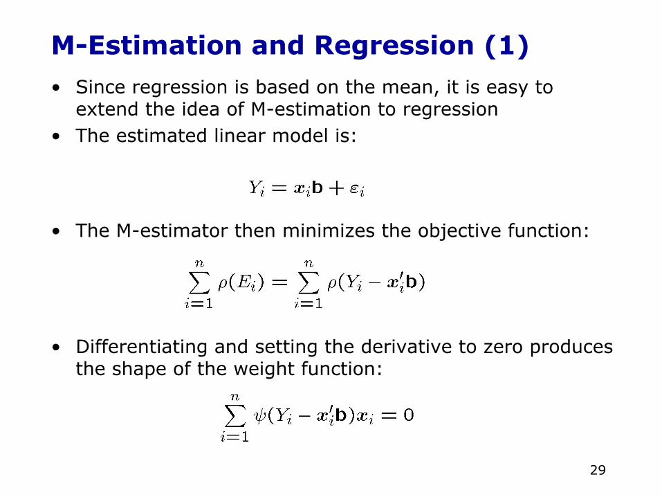
M-Estimation and Regression (1)

• Since regression is based on the mean, it is easy to extend the idea of M-estimation to regression

• The estimated linear model is:

• The M-estimator then minimizes the objective function:

• Differentiating and setting the derivative to zero produces the shape of the weight function:

30

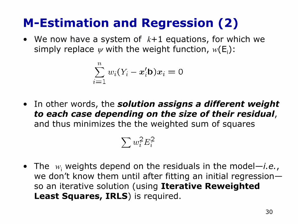
M-Estimation and Regression (2)• We now have a system of k+1 equations, for which we

simply replace ψ with the weight function, w(Ei):

• In other words, the solution assigns a different weight to each case depending on the size of their residual, and thus minimizes the the weighted sum of squares

• The wi weights depend on the residuals in the model—i.e., we don’t know them until after fitting an initial regression—so an iterative solution (using Iterative Reweighted Least Squares, IRLS) is required.

31

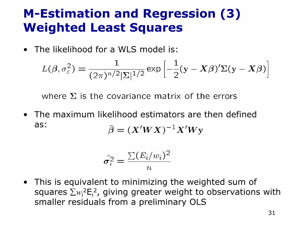
M-Estimation and Regression (3) Weighted Least Squares

• The likelihood for a WLS model is:

• The maximum likelihood estimators are then defined as:

• This is equivalent to minimizing the weighted sum of squares ∑wi

2Ei2, giving greater weight to observations with

smaller residuals from a preliminary OLS

32

M-Estimation and Regression (4)Iterative Reweighted Least Squares• Initial estimates of b are selected using weighted least

squares• The residuals from this model are used to calculate an

estimate of the scale of the residuals S(0) and the weights wi

(0)

• The model is then refit with several iterations minimizing the weighted sum of squares to obtain new estimates of b:

• This process is continued until the model converges (i.e., b(l)' b(l-1))

33

M-Estimation in R (1)Huber Weights

34

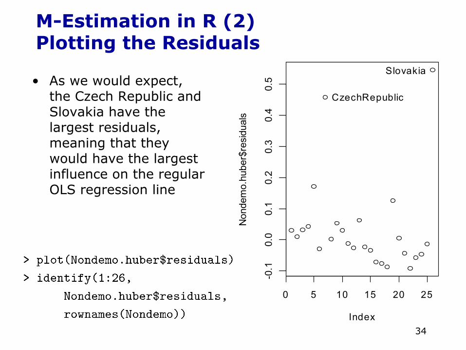
M-Estimation in R (2)Plotting the Residuals

0 5 10 15 20 25

-0.1

0.0

0.1

0.2

0.3

0.4

0.5

Index

Non

dem

o.hu

ber$

resi

dual

s

CzechRepublic

Slovakia• As we would expect,

the Czech Republic and Slovakia have the largest residuals, meaning that they would have the largest influence on the regular OLS regression line

35

M-Estimation in R (3) Examining the weights

• The plot shows the weight given to each case

• In line with the previous graph, the Czech Republic and Slovakia received the least weight of all the observations

• Note:This technique can also be used to assess influential cases

0 5 10 15 20 25

0.2

0.4

0.6

0.8

1.0

Index

Hub

er W

eigh

t

Chile

CzechRepublic

Uruguay

Slovakia

36

M-Estimation in R (4)Bisquare Weights

37

M-Estimation in R (5)Examining the weights

• Again the weights accorded to observations are as expected, and the relative size of the weights match those of the Huber estimates

0 5 10 15 20 25

0.0

0.2

0.4

0.6

0.8

1.0

Index

Bisq

uare

Wei

ght

Chile

CzechRepublic

Uruguay

Slovakia

38

Comparing the Huber and Bisquare weights

0.0 0.2 0.4 0.6 0.8 1.0

0.0

0.2

0.4

0.6

0.8

1.0

Comparison of weights

Bisquare weight

Hub

er w

eigh

t

• Notice that although the relative weights are similar, the Huber method gives a weight of 1 to far more cases than does the bisquare weight

39

Bounded-Influence Regression and the Breakdown Point• M-Estimators are statistically equally efficient as OLS if

the distribution is normal, while at the same time are more robust with respect to influential cases

• Nonetheless, M-estimation can still be influenced by a single very extreme X-value—i.e., like OLS, it still has a breakdown point of 0

• Least-trimmed-squares (LTS) estimators can have a breakdown point up to 50%—i.e., half the data can be influential in the OLS sense before the LTS estimator is seriously affected– Least-trimmed-squares essentially proceeds with OLS

after eliminating the most extreme positive or negative residuals

40

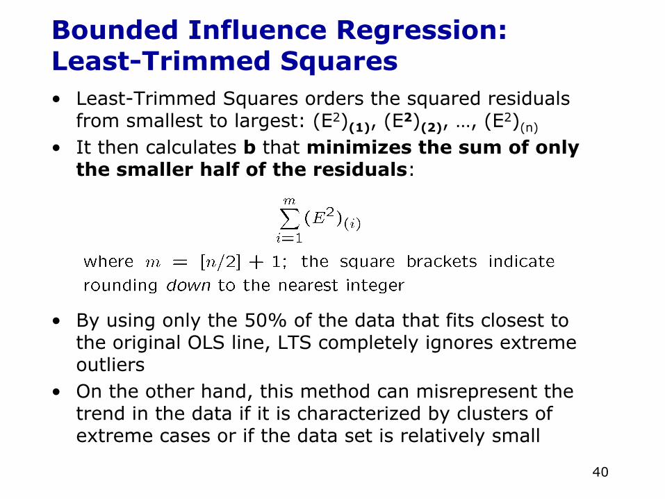
Bounded Influence Regression:Least-Trimmed Squares• Least-Trimmed Squares orders the squared residuals

from smallest to largest: (E2)(1), (E2)(2), …, (E2)(n)

• It then calculates b that minimizes the sum of only the smaller half of the residuals:

• By using only the 50% of the data that fits closest to the original OLS line, LTS completely ignores extreme outliers

• On the other hand, this method can misrepresent the trend in the data if it is characterized by clusters of extreme cases or if the data set is relatively small

41

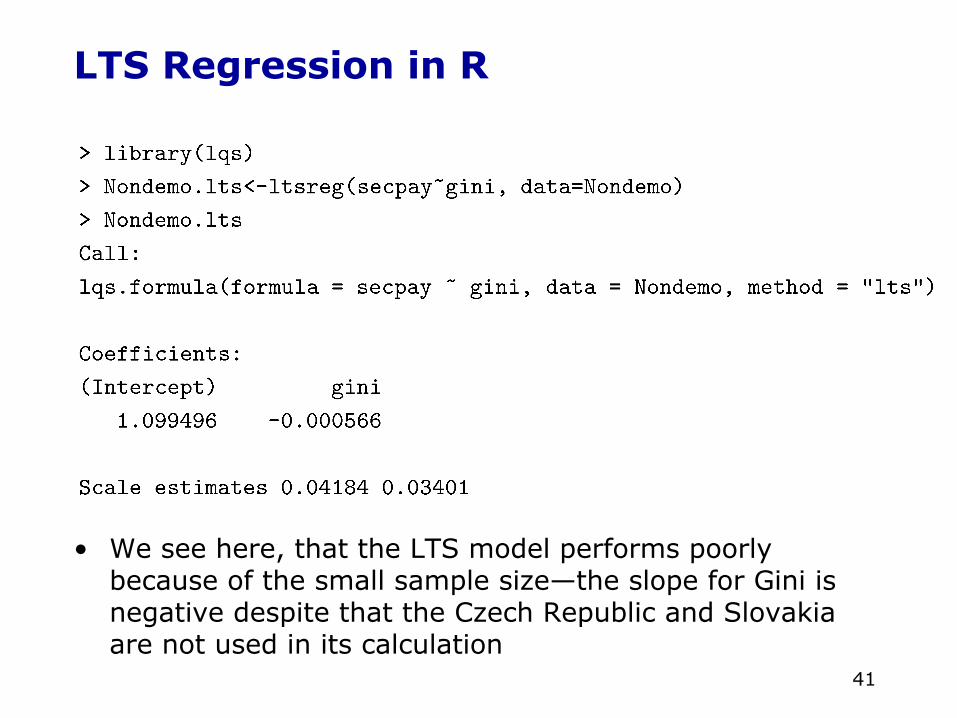
LTS Regression in R

• We see here, that the LTS model performs poorly because of the small sample size—the slope for Gini is negative despite that the Czech Republic and Slovakia are not used in its calculation

42

Bounded Influence Regression:Least- Median Squares

• An alternative bounded influence method is Least Median Squares

• Rather than minimize the sum of the least squares function, this model minimizes the median of the squared residuals, Ei

2

• LMS is very robust with respect to outliers both in terms of X and Y values

• It performs poorly form the point of view of asymptotic efficiency, however

43

LMS Regression in R

• Like the LTS model, this model performs poorly because the sample size is so small

44

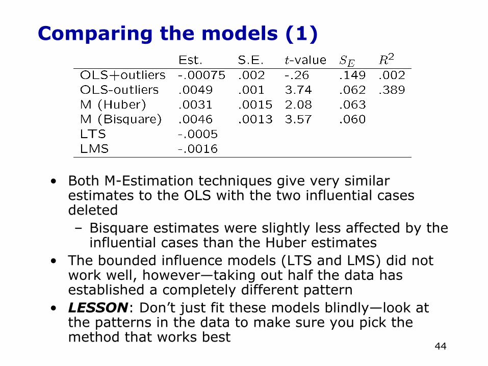
Comparing the models (1)

• Both M-Estimation techniques give very similar estimates to the OLS with the two influential cases deleted– Bisquare estimates were slightly less affected by the

influential cases than the Huber estimates• The bounded influence models (LTS and LMS) did not

work well, however—taking out half the data has established a completely different pattern

• LESSON: Don’t just fit these models blindly—look at the patterns in the data to make sure you pick the method that works best

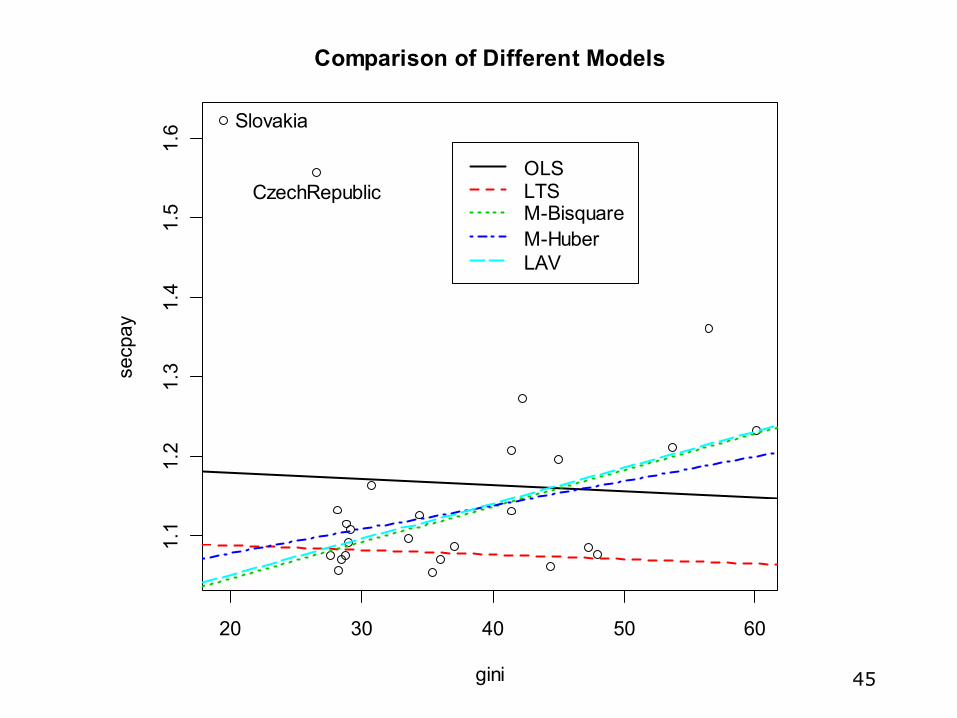
45

20 30 40 50 60

1.1

1.2

1.3

1.4

1.5

1.6

gini

secp

ay

CzechRepublic

Slovakia

OLSLTSM-BisquareM-HuberLAV

Comparison of Different Models

46

R script for comparison plot

47

Summary and Conclusions (1)• Separated points can have a strong influence on

statistical models– Unusual cases can substantially influence the fit of the

OLS model—Cases that are both outliers and high leverage exert influence on both the slopes and intercept of the model

– Outliers may also indicate that our model fails to capture important characteristics of the data

• Efforts should be made to remedy the problem of unusual cases before proceeding to robust regression

• If robust regression is used, careful attention must be paid to the model—different procedures can give completely different answers

48

Summary and Conclusions (2)

• No one robust regression technique is best for all data• There are some considerations, but even these do not

hold up all the time: – LAV regression should generally be avoided because it

is less efficient than other techniques and often not very resistant

– Bounded influence regression models, which can have a breaking point as high as 50%, often work very well with large datasets• They tend to perform poorly with small datasets,

however– M-Estimation is typically better for small datasets, but

its standard errors are not reliable for small samples• This can be overcome by using boot-strapping to

obtain new estimates of the standard errors