Goldsman — ISyE 6739 Linear Regression

REGRESSION

12.1 Simple Linear Regression Model

12.2 Fitting the Regression Line

12.3 Inferences on the Slope Parameter

1

Goldsman — ISyE 6739 12.1 Simple Linear Regression Model

Suppose we have a data set with the following paired

observations:

(x1, y1), (x2, y2), . . . , (xn, yn)

Example:

xi = height of person iyi = weight of person i

Can we make a model expressing yi as a function of

xi?

2

Goldsman — ISyE 6739 12.1 Simple Linear Regression Model

Estimate yi for fixed xi. Let’s model this with the

simple linear regression equation,

yi = β0 + β1xi + εi,

where β0 and β1 are unknown constants and the error

terms are usually assumed to be

ε1, . . . , εniid∼ N(0, σ2)

⇒ yi ∼ N(β0 + β1xi, σ2).

3

Goldsman — ISyE 6739 12.1 Simple Linear Regression Model

y = β0 + β1xwith “high” σ2

y = β0 + β1xwith “low” σ2

4

Goldsman — ISyE 6739 12.1 Simple Linear Regression Model

Warning! Look at data before you fit a line to it:

doesn’t look very linear!

5

Goldsman — ISyE 6739 12.1 Simple Linear Regression Model

xi yiProduction Electric Usage($ million) (million kWh)

Jan 4.5 2.5Feb 3.6 2.3Mar 4.3 2.5Apr 5.1 2.8May 5.6 3.0Jun 5.0 3.1Jul 5.3 3.2Aug 5.8 3.5Sep 4.7 3.0Oct 5.6 3.3Nov 4.9 2.7Dec 4.2 2.5

6

Goldsman — ISyE 6739 12.1 Simple Linear Regression Model

3.5 4.0 4.5 5.0 5.5 6.0

2.2

2.6

3.0

3.4

xi

yi

Great... but how do you fit the line?

7

Goldsman — ISyE 6739 12.2 Fitting the Regression Line

Fit the regression line y = β0 + β1x to the data

(x1, y1), . . . , (xn, yn)

by finding the “best” match between the line and the

data. The “best”choice of β0, β1 will be chosen to

minimize

Q =n∑

i=1(yi − (β0 + β1xi))

2 =n∑

i=1ε2i .

8

Goldsman — ISyE 6739 12.2 Fitting the Regression Line

This is called the least square fit. Let’s solve...

∂Q∂β0

= −2∑

(yi − (β0 + β1xi)) = 0

∂Q∂β1

= −2∑

xi(yi − (β0 + β1xi)) = 0

⇔ ∑

yi = nβ0 + β1∑

xi∑

xiyi = −2∑

xi(yi − (β0 + β1xi)) = 0

After a little algebra, get

β1 = n∑

xiyi−(∑

xi)(∑

yi)n

∑x2

i −(∑

xi)2

β0 = y − β1x, where y ≡ 1n

∑

yi and x ≡ 1n

∑

xi.

9

Goldsman — ISyE 6739 12.2 Fitting the Regression Line

Let’s introduce some more notation:

Sxx =∑

(xi − x)2 =∑

x2i − nx2

=∑

x2i − (

∑xi)

2

n

Sxy =∑

(xi − x)(yi − y) =∑

xiyi − nxy

=∑

xiyi − (∑

xi)(∑

yi)n

These are called “sums of squares.”

10

Goldsman — ISyE 6739 12.2 Fitting the Regression Line

Then, after a little more algebra, we can write

β1 =Sxy

Sxx

Fact: If the εi’s are iid N(0, σ2), it can be shown that

β0 and β1 are the MLE’s for β0 and β1, respectively.

(See text for easy proof).

Anyhow, the fitted regression line is:

y = β0 + β1x.

11

Goldsman — ISyE 6739 12.1 Simple Linear Regression Model

Fix a specific value of the explanatory variable x∗, the

equation gives a fitted value y|x∗ = β0 + β1x∗ for the

dependent variable y.

12

y

y = β0 + β1x

x∗ xi

x

y|x∗

Goldsman — ISyE 6739 12.2 Fitting the Regression Line

For actual data points xi, the fitted values are yi =

β0 + β1xi.

observed values : yi = β0 + β1xi + εi

fitted values : yi = β0 + β1xi

Let’s estimate the error variation σ2 by considering

the deviations between yi and yi.

SSE =∑

(yi − yi)2 =

∑

(yi − (β0 + β1xi))2

=∑

y2i − β0

∑

yi − β1∑

xiyi.

13

Goldsman — ISyE 6739 12.2 Fitting the Regression Line

Turns out that σ2 ≡ SSEn−2 is a good estimator for σ2.

Example: Car plant energy usage n = 12,∑12

i=1 xi =

58.62,∑

yi = 34.15,∑

x2i = 291.231,

∑

y2i = 98.697,

∑

xiyi = 169.253

β1 = 0.49883, β0 = 0.4090

⇒ fitted regression line is

y = 0.409 + 0.499x y|5.5 = 3.1535

What about something like y|10.0?

14

Goldsman — ISyE 6739 12.3 Inferences on Slope Parameter β1

β1 =SxySxx

, where Sxx =∑

(xi − x)2 and

Sxy =∑

(xi − x)(yi − y) =∑

(xi − x)yi − y∑

(xi − x)

=∑

(xi − x)yi

15

Goldsman — ISyE 6739 12.3 Inferences on Slope Parameter β1

Since the yi’s are independent with yi ∼ N(β0+β1xi, σ2)

(and the xi’s are constants), we have

Eβ1 = 1Sxx

ESxy = 1Sxx

∑

(xi − x)Eyi = 1Xxx

∑

(xi − x)(β0 + β1x

= 1Sxx

[β0∑

(xi − x)︸ ︷︷ ︸

0

+β1∑

(xi − x)xi]

= β1Sxx

∑

(x2i − xix) = β1

Sxx(

∑

x2i − nx2

︸ ︷︷ ︸

Sxx

) = β1

⇒ β1 is an unbiased estimator of β1.

16

Goldsman — ISyE 6739 12.3 Inferences on Slope Parameter β1

Further, since β1 is a linear combination of indepen-

dent normals, β1 is itself normal. We can also derive

Var(β1) =1

S2xx

Var(Sxy) =1

S2xx

∑

(xi−x)2Var(yi) =σ2

Sxx.

Thus, β1 ∼ N(β1, σ2

Sxx)

17

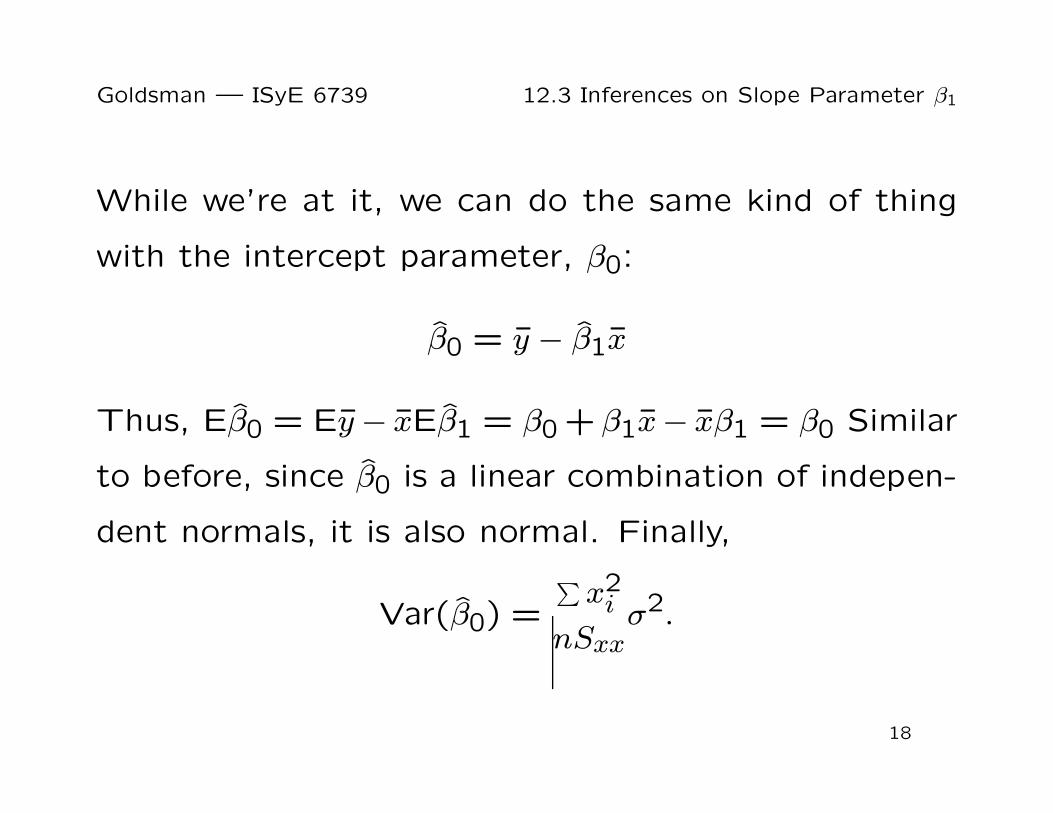
Goldsman — ISyE 6739 12.3 Inferences on Slope Parameter β1

While we’re at it, we can do the same kind of thing

with the intercept parameter, β0:

β0 = y − β1x

Thus, Eβ0 = Ey − xEβ1 = β0 + β1x− xβ1 = β0 Similar

to before, since β0 is a linear combination of indepen-

dent normals, it is also normal. Finally,

Var(β0) =

∑

x2i

nSxxσ2.

18

Goldsman — ISyE 6739 12.3 Inferences on Slope Parameter β1

Proof:

Cov(y, β1) = 1Sxx

Cov(y,∑

(xi − x)yi)

=∑

(xi−xSxx

)Cov(y, yi)

=∑

(xi−x)Sxx

σ2

n = 0

⇒ Var(β0) = Var(y − β1x)

= Var(y) + x2Varβ1 − 2xCov(y, β1)︸ ︷︷ ︸

0

= σ2

n + x2 σ2

Sxx

= σ2(

Sxx−nx2

nSxx

)

.

Thus, β0 ∼ N(β0,∑

x2i

nSxxσ2).

19

Goldsman — ISyE 6739 12.3 Inferences on Slope Parameter β1

Back to β1 ∼ N(β1, σ2/Sxx) . . .

⇒ β1 − β1√

σ2/Sxx∼ N(0,1)

Turns out:

(1) σ2 = SSEn−2 ∼ σ2χ2(n−2)

n−2 ;

(2) σ2 is independent of β1.

20

Goldsman — ISyE 6739 12.3 Inferences on Slope Parameter β1

⇒β1−β1σ/

√Sxx

σ/σ∼ N(0,1)

√

χ2(n−2)n−2

∼ t(n − 2)

⇒β1 − β1

σ/√

Sxx∼ t(n − 2).

21

Goldsman — ISyE 6739 12.3 Inferences on Slope Parameter β1

1 − α

t(n − 2)

−tα/2,n−2 tα/2,n−2

22

Goldsman — ISyE 6739 12.3 Inferences on Slope Parameter β1

2-sided Confidence Intervals for β1:

1 − α = Pr(−tα/2,n−2 ≤ β1−β1σ/

√Sxx

≤ tα/2,n−2)

= Pr(β1 − tα/2,n−2σ√Sxx

≤ β1 ≤ β1 + tα/2,n−2σ√Sxx

)

1-sided CI’s for β1:

β1 ∈ (−∞, β1 + tα,n−2σ√Sxx

)

β1 ∈ (β1 − tα,n−2σ√Sxx

,∞)

23