Embed Size (px)
Citation preview

Regression Analysis of Caterpillar 793D HaulTruck Engine Failure Data and Through-Life
Diagnostic Information Using the ProportionalHazards Model
by
Wiehahn Alwyn Carstens
Thesis presented in partial fulfilment of the requirements forthe degree of Master of Science in Industrial Engineering at
Stellenbosch University
Department of Industrial Engineering,University of Stellenbosch,
Private Bag X1, Matieland 7602, South Africa.
Supervisor: Dr. P.J. Vlok, Prof. C.S.L. Schutte and T. Visser
March 2012

Declaration
By submitting this thesis electronically, I declare that the entirety of the workcontained therein is my own, original work, that I am the owner of the copy-right thereof (unless to the extent explicitly otherwise stated) and that I have notpreviously in its entirety or in part submitted it for obtaining any qualification.
Date: . . . . . . . . . . . . . . . . . . . . . . . . . . . . . . . . .
Copyright © 2012 Stellenbosch UniversityAll rights reserved.
i
Stellenbosch University http://scholar.sun.ac.za

Abstract
Regression Analysis of Caterpillar 793D Haul Truck EngineFailure Data and Through-Life Diagnostic Information
Using the Proportional Hazards ModelW.A. Carstens
Department of Industrial Engineering,University of Stellenbosch,
Private Bag X1, Matieland 7602, South Africa.
Thesis: MScEng (Industrial)March 2012
Physical Asset Management (PAM) is becoming a greater concern for compa-nies in industry today. The widely accepted British Standards Institutes’ specifi-cation for optimized management of physical assets and infrastructure is PAS55.According to PAS55, PAM is the “systematic and co-ordinated activities and prac-tices through which an organization optimally manages its physical assets, andtheir associated performance, risks and expenditures over their life cycle for thepurpose of achieving its organizational strategic plan”.
One key performance area of PAM is Asset Care Plans (ACP). These plansare maintenance strategies which improve or ensure acceptable asset reliabilityand performance during its useful life. Maintenance strategies such as ConditionBased Maintenance (CBM) acts upon Condition Monitoring (CM) data, disre-garding the previous failure histories of an asset. Other maintenance strategies,such as Usage Based Maintenance (UBM), is based on previous failure histories,and does not consider CM data.
Regression models make use of both CM data and previous failure historiesto develop a model which represents the underlying failure behaviour of the assetunder study. These models can be of high value in ACP development due to thefact that Residual Useful Life (RUL) can be estimated and/or the long term life
ii
Stellenbosch University http://scholar.sun.ac.za

ABSTRACT iii
cycle cost can be optimized.
The objective of this thesis was to model historical failure data and CM datawell enough so that RUL or optimized preventive maintenance instant estimationscan be made. These estimates were used in decision models to develop mainte-nance schedules, i.e. ACPs.
Several regression models were evaluated to determine the most suitable modelto achieve the objectives of this thesis. The model found to be most suitable forthis research project was the Proportional Hazards Model (PHM). A comprehen-sive investigation on the PHM was undertaken focussing on the mathematics andthe practical implementation thereof.
Data obtained from the South African mining industry was modelled with theWeibull PHM. It was found that the developed model produced estimates whichwere accurate representations of reality. These findings provide an exciting basisfor the development of future Weibull PHMs that could result in huge maintenancecost savings and reduced failure occurrences.
Stellenbosch University http://scholar.sun.ac.za

Uittreksel
Regressie Analise van Caterpillar 793D Trok Enjin FalingsData en Gedokumenterde Toestands Moniterings Data Met
Gebruik van die Proporsionele Gevaarkoers Model.(“Regression Analysis of Caterpillar 793D Haul Truck Failure Data and Through-Life
Diagnostic Information Using the Proportional Hazards Model”)
W.A. CarstensDepartement Bedryfs Ingenieurswese,
Universiteit van Stellenbosch,Privaatsak X1, Matieland 7602, Suid Afrika.
Tesis: MScIng (Bedryfs)Maart 2012
Fisiese Bate Bestuur (FBB) is besig om ’n groter bekommernis vir maatskappyein die bedryf te word. Die Britse Standaarde Instituut se spesifikasie vir optimalebestuur van fisiese bates en infrastruktuur is PAS55. Volgens PAS55 is FBB die“sistematiese en gekoördineerde aktiwiteite en praktyke wat deur ’n organisasieoptimaal sy fisiese bates, hul verwante prestasie, risiko’s en uitgawes vir die doelvan die bereiking van sy organisatoriese strategiese plan beheer oor hul volle le-wensiklus te bestuur”.
Een Sleutel Fokus Area (SFA) van FBB is Bate Versorgings Plan (BVP) ont-wikkeling. Hierdie is onderhouds strategieë wat bate betroubaarheid verbeter ofverseker tydens die volle bruikbare lewe van die bate. Een onderhoud strategieis Toestands Gebasseeerde Onderhoud (TGO) wat besluite baseer op ToestandMonitering (TM) informasie maar neem nie die vorige falingsgeskiedenis van diebate in ag nie. Ander onderhoud strategieë soos Gebruik Gebasseerde Onderhoud(GGO) is gebaseer op historiese falingsdata maar neem nie TM inligting in ag nie.
Regressiemodelle neem beide TM data en historiese falings geskiedenis data inag ten einde die onderliggende falings gedrag van die gegewe bate te verteenwoor-
iv
Stellenbosch University http://scholar.sun.ac.za

UITTREKSEL v
dig. Hierdie modelle kan baie nuttig wees vir BVP ontwikkeling te danke aan diefeit dat Bruikbare Oorblywende Lewe (BOL) geskat kan word en/of die langter-myn lewenssilus koste geoptimeer kan word.
Die doelwit van hierdie tesis was om historiese falingsdata en TT data goedgenoeg te modelleer sodat BOL of optimale langtermyn lewensiklus kostes bepaalkan word om opgeneem te word in BVP ontwikkeling. Hierdie bepalings word dangebruik in besluitnemings modelle wat gebruik kan word om onderhoud skedulesop te stel, d.w.s. om ’n BVP te ontwikkel.
Verskeie regressiemodelle was geëvalueer om die regte model te vind waarmeedie doel van hierdie tesis te bereik kan word. Die mees geskikte model vir die na-vorsingsprojek was die Proporsionele Gevaarkoers Model (PGM). ’n Omvattendeondersoek oor die PGM is onderneem wat fokus op die wiskunde en die praktieseimplementering daarvan.
Data is van die Suid-Afrikaanse mynbedryf verkry en is gemodelleer met be-hulp van die Weibull PGM. Dit was bevind dat die ontwikkelde model resultategeproduseer het wat ’n akkurate verteenwoordinging van realiteit is. Hierdie be-vindinge bied ’n opwindende basis vir die ontwikkeling van toekomstige WeibullProporsionele Gevaarkoers Modelle wat kan lei tot groot onderhoudskoste bespa-rings en minder onverwagte falings.
Stellenbosch University http://scholar.sun.ac.za

Acknowledgements
I would like to express my sincere gratitude to the following people and organisa-tions:
• Dr. PJ Vlok, my study leader, for his support, dedicated guidance and thetime he invested in this research project; which allowed and motivated meto meet ambitious personal deadlines;
• Ernest Stonestreet of Anglo American, for sponsoring me to visit Sishen andobtain data;
• Louis Vlok, for his support;
• Prof. Corne Schutte and Tanya Visser for their supervision and guidance.
• My family, for their continued support;
• Our heavenly Father, for giving me the strength and determination to com-plete this project.
The AuthorDecember, 2011
vi
Stellenbosch University http://scholar.sun.ac.za

Contents
Declaration i
Abstract ii
Uittreksel iv
Acknowledgements vi
Contents vii
List of Figures x
List of Tables xii
Nomenclature xiii
Glossary xv
1 Introduction 11.1 Introduction . . . . . . . . . . . . . . . . . . . . . . . . . . . . . . . 11.2 Problem Statement . . . . . . . . . . . . . . . . . . . . . . . . . . . 11.3 Research Objectives . . . . . . . . . . . . . . . . . . . . . . . . . . . 31.4 Research Methodology . . . . . . . . . . . . . . . . . . . . . . . . . 3
2 Literature Review and Contextualization of the Problem 52.1 Introduction . . . . . . . . . . . . . . . . . . . . . . . . . . . . . . . 5
2.1.1 Asset Care Plans . . . . . . . . . . . . . . . . . . . . . . . . 72.2 Condition Based Maintenance . . . . . . . . . . . . . . . . . . . . . 14
2.2.1 Data Acquisition . . . . . . . . . . . . . . . . . . . . . . . . 162.2.2 Data Preparation . . . . . . . . . . . . . . . . . . . . . . . . 172.2.3 Decision Making . . . . . . . . . . . . . . . . . . . . . . . . 17
2.3 Failure data analysis . . . . . . . . . . . . . . . . . . . . . . . . . . 23
vii
Stellenbosch University http://scholar.sun.ac.za

CONTENTS viii
2.3.1 Model type selection . . . . . . . . . . . . . . . . . . . . . . 252.3.2 Censored data . . . . . . . . . . . . . . . . . . . . . . . . . . 282.3.3 Reliability Theory . . . . . . . . . . . . . . . . . . . . . . . 282.3.4 Regression Modelling . . . . . . . . . . . . . . . . . . . . . . 34
2.4 Conclusion . . . . . . . . . . . . . . . . . . . . . . . . . . . . . . . . 35
3 Regression models 363.1 Introduction . . . . . . . . . . . . . . . . . . . . . . . . . . . . . . . 363.2 Proportional Odds Models . . . . . . . . . . . . . . . . . . . . . . . 383.3 Additive Hazards Model . . . . . . . . . . . . . . . . . . . . . . . . 413.4 Proportional Hazards Model . . . . . . . . . . . . . . . . . . . . . . 433.5 Accelerated Failure Time Model . . . . . . . . . . . . . . . . . . . . 463.6 Proportional Intensity Models . . . . . . . . . . . . . . . . . . . . . 513.7 Extended Hazard Regression Model . . . . . . . . . . . . . . . . . . 523.8 Model Selection . . . . . . . . . . . . . . . . . . . . . . . . . . . . . 553.9 Conclusion . . . . . . . . . . . . . . . . . . . . . . . . . . . . . . . . 55
4 Proportional Hazards Model 564.1 Introduction . . . . . . . . . . . . . . . . . . . . . . . . . . . . . . . 564.2 Censoring . . . . . . . . . . . . . . . . . . . . . . . . . . . . . . . . 574.3 Semi-parametric PHM . . . . . . . . . . . . . . . . . . . . . . . . . 60
4.3.1 Maximum Likelihood Estimate . . . . . . . . . . . . . . . . 614.3.2 Marginal Likelihood . . . . . . . . . . . . . . . . . . . . . . 624.3.3 Partial Likelihood . . . . . . . . . . . . . . . . . . . . . . . . 63
4.4 Fully-parametric PHM . . . . . . . . . . . . . . . . . . . . . . . . . 654.4.1 Model . . . . . . . . . . . . . . . . . . . . . . . . . . . . . . 654.4.2 Regression Coefficient Estimation . . . . . . . . . . . . . . . 66
4.5 Model Fitting Procedure Of the Fully-Parametric Proportional Haz-ards Model . . . . . . . . . . . . . . . . . . . . . . . . . . . . . . . 674.5.1 Artificial Bee Colony Optimization . . . . . . . . . . . . . . 694.5.2 Evaluation of Artificial Bee Colony Optimization Success . . 71
4.6 Goodness-of-fit tests . . . . . . . . . . . . . . . . . . . . . . . . . . 734.6.1 Analytical Techniques . . . . . . . . . . . . . . . . . . . . . 744.6.2 Graphical Techniques . . . . . . . . . . . . . . . . . . . . . . 76
4.7 Decision Model . . . . . . . . . . . . . . . . . . . . . . . . . . . . . 794.7.1 Residual Life Estimation . . . . . . . . . . . . . . . . . . . . 794.7.2 Decision Making Rule With Residual Life Estimation . . . . 824.7.3 Cost Optimization Models . . . . . . . . . . . . . . . . . . . 824.7.4 Final Decision Model . . . . . . . . . . . . . . . . . . . . . . 85
4.8 Conclusion . . . . . . . . . . . . . . . . . . . . . . . . . . . . . . . . 85
Stellenbosch University http://scholar.sun.ac.za

CONTENTS ix
5 Proportional Hazards Model Application 865.1 Introduction . . . . . . . . . . . . . . . . . . . . . . . . . . . . . . . 865.2 Data Requirements . . . . . . . . . . . . . . . . . . . . . . . . . . . 87
5.2.1 Events . . . . . . . . . . . . . . . . . . . . . . . . . . . . . . 875.2.2 Covariates . . . . . . . . . . . . . . . . . . . . . . . . . . . . 885.2.3 Requirements . . . . . . . . . . . . . . . . . . . . . . . . . . 88
5.3 CAT 793D Data . . . . . . . . . . . . . . . . . . . . . . . . . . . . . 895.3.1 On-Board Measurements . . . . . . . . . . . . . . . . . . . . 905.3.2 Oil Analysis . . . . . . . . . . . . . . . . . . . . . . . . . . . 915.3.3 Maintenance Decisions . . . . . . . . . . . . . . . . . . . . . 92
5.4 Weibull PHM Fit . . . . . . . . . . . . . . . . . . . . . . . . . . . . 935.4.1 Data Manipulation . . . . . . . . . . . . . . . . . . . . . . . 935.4.2 Covariate Selection . . . . . . . . . . . . . . . . . . . . . . . 955.4.3 Goodness-of-fit Tests . . . . . . . . . . . . . . . . . . . . . . 975.4.4 Final Model . . . . . . . . . . . . . . . . . . . . . . . . . . . 104
5.5 Model Validation Data . . . . . . . . . . . . . . . . . . . . . . . . . 1045.5.1 Decision Model . . . . . . . . . . . . . . . . . . . . . . . . . 1065.5.2 Decision model 1: Residual Useful Life Estimates . . . . . . 1085.5.3 Decision model 2: Long Term Cost Optimization . . . . . . 1145.5.4 Decision model 3: Combining decision model 1 and decision
model 2. . . . . . . . . . . . . . . . . . . . . . . . . . . . . . 1225.6 Model Validation . . . . . . . . . . . . . . . . . . . . . . . . . . . . 1225.7 Conclusion . . . . . . . . . . . . . . . . . . . . . . . . . . . . . . . . 125
6 Conclusion and Recommendations 1266.1 Overview . . . . . . . . . . . . . . . . . . . . . . . . . . . . . . . . . 1266.2 Recommendations for Future Research . . . . . . . . . . . . . . . . 128
List of References 129
Appendices 138
Data 139
Long Term Cost Optimization Decision Model 143
Stellenbosch University http://scholar.sun.ac.za

List of Figures
2.1 Bathtub curve. . . . . . . . . . . . . . . . . . . . . . . . . . . . . . . . 92.2 Failure rate graphs of typical mechanical and electronic systems. . . . . 102.3 Failure progression graph indicating PF interval. . . . . . . . . . . . . . 112.4 Physical Asset Management and the associated maintenance strategies. 122.5 Diagnostics and its elements. . . . . . . . . . . . . . . . . . . . . . . . 192.6 Prognostics and its elements. . . . . . . . . . . . . . . . . . . . . . . . 202.7 Failure time measurement (Adapted from Vlok (2001)). . . . . . . . . . 242.8 Framework for statistical failure data analysis. (Adapted from Louit
et al. (2009) and Coetzee (1997)). . . . . . . . . . . . . . . . . . . . . . 262.9 Graphical illustration of GAN assumption. . . . . . . . . . . . . . . . . 322.10 Graphical illustration of BAO assumption. . . . . . . . . . . . . . . . . 33
3.1 Graphical illustration of how the covariate influence diminish over time. 393.2 Graphical illustration of the AHM. . . . . . . . . . . . . . . . . . . . . 423.3 Graphical illustration of the proportional FOM assumption. . . . . . . 443.4 Different TR values and how it affects the failure probability time-scale
of an item. . . . . . . . . . . . . . . . . . . . . . . . . . . . . . . . . . . 483.5 Baseline Foce Of Mortality estimation using quadratic splines. . . . . . 53
4.1 Three types of Random censoring. . . . . . . . . . . . . . . . . . . . . . 594.2 ABC algorithm solution plot. . . . . . . . . . . . . . . . . . . . . . . . 724.3 Typical Cox-Snell residual plot. . . . . . . . . . . . . . . . . . . . . . . 784.4 Illustration of RUL of non-repairable items. . . . . . . . . . . . . . . . 814.5 Optimal maintenance instant. . . . . . . . . . . . . . . . . . . . . . . . 834.6 Long term cost per unit time optimization. . . . . . . . . . . . . . . . . 84
5.1 Cat 793D haul truck. . . . . . . . . . . . . . . . . . . . . . . . . . . . . 895.2 Extrapolation of oil data. . . . . . . . . . . . . . . . . . . . . . . . . . 945.3 Extrapolation of oil data. . . . . . . . . . . . . . . . . . . . . . . . . . 965.4 Covariate combination: Fe, boost pressure, left exhaust temperature
and engine filter oil pressure (min). . . . . . . . . . . . . . . . . . . . . 100
x
Stellenbosch University http://scholar.sun.ac.za

LIST OF FIGURES xi
5.5 Covariate combination: Fe, right after cooler temperature and enginecoolant temperature. . . . . . . . . . . . . . . . . . . . . . . . . . . . . 101
5.6 Covariate combination: Fe, boost pressure and left exhaust temp. . . . 1035.7 Extrapolation of boost pressure data into the future. . . . . . . . . . . 1065.8 Extrapolation of left exhaust temperature data into the future. . . . . . 1075.9 Validation truck event 1. . . . . . . . . . . . . . . . . . . . . . . . . . . 1095.10 Validation truck event 2. . . . . . . . . . . . . . . . . . . . . . . . . . . 1105.11 Validation truck event 3. . . . . . . . . . . . . . . . . . . . . . . . . . . 1125.12 Validation truck event 4. . . . . . . . . . . . . . . . . . . . . . . . . . . 1135.13 Validation truck event 5. . . . . . . . . . . . . . . . . . . . . . . . . . . 1155.14 Long term cost optimization function for event 1. . . . . . . . . . . . . 1165.15 Long term cost optimization function for event 2. . . . . . . . . . . . . 1175.16 Long term cost optimization function for event 3. . . . . . . . . . . . . 1195.17 Long term cost optimization function for event 4. . . . . . . . . . . . . 1205.18 Long term cost optimization function for event 5. . . . . . . . . . . . . 1215.19 Decision model estimations compared to actual event times. . . . . . . 124
1 Cost function for the first inspection of the first event. . . . . . . . . . 1442 Cost function for the second inspection of the first event. . . . . . . . . 1453 Cost function for the first inspection of the second event. . . . . . . . . 1464 Cost function for the second inspection of the second event. . . . . . . 1475 Cost function for the first inspection of the third event. . . . . . . . . . 1486 Cost function for the second inspection of the third event. . . . . . . . 1497 Cost function for the first inspection of the fourth event. . . . . . . . . 1508 Cost function for the second inspection of the fourth event. . . . . . . . 1519 Cost function of the fifth event. . . . . . . . . . . . . . . . . . . . . . . 152
Stellenbosch University http://scholar.sun.ac.za

List of Tables
3.1 Regression model evaluation matrix. . . . . . . . . . . . . . . . . . . . 373.2 Proportional Odds Model evaluation. . . . . . . . . . . . . . . . . . . . 403.3 Additive Hazards Model evaluation. . . . . . . . . . . . . . . . . . . . . 433.4 Proportional Hazards Model evaluation. . . . . . . . . . . . . . . . . . 463.5 Accelerated Failure Time Model evaluation. . . . . . . . . . . . . . . . 503.6 Proportional Intensity Model evaluation. . . . . . . . . . . . . . . . . . 523.7 Extended Hazard Regression Model evaluation. . . . . . . . . . . . . . 543.8 Selection of most suitable regression model. . . . . . . . . . . . . . . . 55
4.1 Goodness-if-fit Tests . . . . . . . . . . . . . . . . . . . . . . . . . . . . 74
5.1 Event table. . . . . . . . . . . . . . . . . . . . . . . . . . . . . . . . . . 975.2 An extract of the 16th event’s measured covariates. . . . . . . . . . . . 985.3 Covariate combination: Fe, boost pressure, left exhaust temperature
and engine oil pressure. . . . . . . . . . . . . . . . . . . . . . . . . . . . 995.4 Covariate combination: Fe, right after cooler temperature and engine
coolant temperature. . . . . . . . . . . . . . . . . . . . . . . . . . . . . 1025.5 Covariate combination: Fe, boost pressure and left exhaust temp. . . . 1025.6 Kolmogorov-Smirnoff values. . . . . . . . . . . . . . . . . . . . . . . . . 1045.7 Validation truck event’s table. . . . . . . . . . . . . . . . . . . . . . . . 1055.8 Criteria 1 and 2 combination. . . . . . . . . . . . . . . . . . . . . . . . 123
1 Event table. . . . . . . . . . . . . . . . . . . . . . . . . . . . . . . . . . 1412 On-board data and tribology data. . . . . . . . . . . . . . . . . . . . . 142
xii
Stellenbosch University http://scholar.sun.ac.za

Nomenclature
β Weibull shape parameterη Weibull scale parameterγ Row vector containing regression coefficientsι(t) Rate of Occurrence Of Failure as a function of timeλ Functional term dependent on time and covariatesz(x) Covariate vector dependent on timea Time required to perform preventive maintenanceb Time required to perform maintenance after unexpected failure occurredCXc Cost of CorrectiveCXp Cost of preventive maintenanceC(Xp) Total cost per unit time as a function of Xp
E Expected valuef Probability density distributionF Cumulative failure distributionh Force of mortalityH Cumulative Force Of MortalityL Likelihoodm Total number of observed failuresN(t) Observed number of failures at time t
n Observed number of failuresP Probabilityr Total number of observed eventsR Reliability functiont Continuous timeTi ith Discrete repair time
xiii
Stellenbosch University http://scholar.sun.ac.za

NOMENCLATURE xiv
x Continuous global timeXi ith Discrete event time measured in local timeXp Recommended preventive replacement timeXc Inspection periodXr+1 Upper confidence limit of the Residual Life EstimationX∼
r+1Lower confidence limit of the Residual Life Estimation
Stellenbosch University http://scholar.sun.ac.za

Glossary
ACP Asset Care PlansAFTM Accelerated Failure Time ModelAHM Additive Hazards ModelBAO Bad As OldBOWN Bad as Old but Worse than NewCM Condition MonitoringCBM Condition Based MaintenanceCMMS Computerized Maintenance Management SystemDIM Design Improvement MaintenanceEAMS Engineering Asset Management SystemEHRM Extended Hazard Regression ModelEHS Environmental Health and SafetyFOM Force Of MortalityGAN Good As NewHMM Hidden Markov ModelHPP Homogeneous Poison ProcessIID Independent Identical DistributionISO International Organization for StandardizationKPA Key Performance AreaLCC Life Cycle CostML Marginal LikelihoodMLE Maximum Likelihood EstimateNHPP Non-homogeneous Poison ProcessPAM Physical Asset ManagementPAS55 Publicly Available Specification 55PF Potential-FailurePHM Proportional Hazards ModelPIM Proportional Intensity ModelPL Partial LikelihoodROCOF Rate of Occurrence Of Failure
xv
Stellenbosch University http://scholar.sun.ac.za

GLOSSARY xvi
ROI Return On InvestmentRP Renewal ProcessRUL Residual Useful LifeRULE Residual Useful Life ExpectedTR Time RatioTTT Total Time on TestUBM Usage Based MaintenanceWO Worse than Old
Stellenbosch University http://scholar.sun.ac.za

Chapter 1
Introduction
1.1 IntroductionIndustry has only recently started to realize the importance of optimized main-tenance activities. According to Mobley (2002), although maintenance is one ofthe driving factors behind reliable and efficient operation, many industries stillknowingly perform ineffective maintenance actions.
Heng (2000) states that the annual maintenance expenditure in American com-panies in the year 2000 was approximately $1.2 trillion which consisted of roughly50% wasted expenditure. This was also shown by Heng et al. (2009) indicat-ing that up to a third of maintenance expenditure is being wasted on ineffectivemaintenance actions. Today’s complex and advanced machines demand highly so-phisticated maintenance strategies in order to sufficiently maintain them.
From this can be seen that a large portion of the total expenditure indus-try spends on maintenance is being wasted on unnecessary maintenance actions.Therefore a need exists to optimize maintenance actions in order to minimize un-necessary maintenance actions. For this reason there is major scope in the SouthAfrican industry to apply Physical Asset Management (PAM) principles to im-prove the overall performance and reliability of assets.
1.2 Problem StatementAn important topic of discussion in industry today is PAM. According to BritishStandards Institutes’ Publicly Availably Specification (PAS55:2008), PAM is thesystematic and co-ordinated activities and practices through which an organizationoptimally manages its assets, and the associated performance risks and expendi-
1
Stellenbosch University http://scholar.sun.ac.za

CHAPTER 1. INTRODUCTION 2
tures over their life cycle for the purpose of achieving its organizational strategicplan. In most cases managing physical assets such that a desired and sustainableobjective is achieved.
In most cases PAM comprises of many different elements such as Work Plan-ning and Control (WPC) and Financial Management (FM). Several other elementsare presented in Chapter 2. Most companies develop their own PAM policies toeffectively and efficiently manage their own assets. To manage assets effectivelyand efficiently, it is vital to maintain these assets. Companies typically developseveral Key Performance Areas (KPAs) which they apply in order to effectivelymanage and maintain an asset to fit its’ specific functional needs.
One KPA of PAM is Asset Care Plan (ACP) development which consists of sev-eral tactical preventive maintenance strategies. Maintenance practitioners mainlyconsider two preventive maintenance strategies. The first being a strategy whichbases its maintenance actions purely on the age of the asset measured in time,kilometers, liters processed, tons or any other process parameter. This type ofmaintenance strategy is one of the most popular strategies found in industry andis formally known as Usage Based Maintenance (UBM).
In the case of UBM, Condition Monitoring (CM) information is disregardedand maintenance is purely based on the previous failure histories. The determinedmaintenance instant should not allow that too much residual life is wasted keepingin mind that extending the maintenance instant increases the probability of failure.
The second popular strategy used in industry is when maintenance action isbased on CM information in which case maintenance is taken when a certaincondition reaches a predefined failure level. This strategy is formally known asCondition Based Maintenance (CBM). This strategy does not take into accountthe asset’s previous failure histories.
Preventive maintenance strategies has the sole purpose of attempting to pre-vent the occurrence of unexpected failure. Unexpected failures have serious con-sequences such as damage to the asset, production losses and in some cases lossof life. Compared to the cost of unexpected failures, preventive maintenance isoften relatively inexpensive in that many of the unwanted financial consequencesare eliminated.
Both of the mentioned maintenance strategies have their own respective ad-vantages. Individually, many studies have been performed to enhance their main-
Stellenbosch University http://scholar.sun.ac.za
CHAPTER 1. INTRODUCTION 3
tenance decision making capability. However, not much work has been done toincorporate both these maintenance strategies into one maintenance decision mak-ing tool. Therefore, the challenge undertaken in this thesis is to investigate modelswhich take into account both CM information and historical failure data whichimprove practical preventive maintenance decision making. This will be done byusing the methodology given in Section 1.4.
1.3 Research ObjectivesThe objective of this research project is to master the relevant literature in order togain a detailed understanding of the model ultimately selected to solve the problemdescribed in the problem statement. The researched theory will be validated byapplying the model to industry data whereby the accuracy of the estimations madewith the model will then be illustrated.
1.4 Research MethodologyIn order to achieve the research objectives given in Section 1.3, the researchmethodology for the following chapters are listed below.
i. Perform a comprehensive literature study on the field of asset managementfocussing on several maintenance strategies and also failure data analysis.Identify suitable mathematical models with which the research objectives canbe achieved.
ii. Evaluate the identified models according to the objectives of this thesis. Themost appropriate model will be selected to accomplish the objectives of thethesis based on the evaluation process.
iii. Perform a comprehensive investigation of the chosen regression model fo-cussing on the mathematics and practical implementation thereof. Study deci-sion making models associated with the selected model with which optimizedmaintenance decisions can be calculated.
iv. Perform a case study whereby the chosen model’s theory is applied to datafound in the South African industry.
v. Conclude with a summary of the thesis findings and some recommendationsfor future research.
Stellenbosch University http://scholar.sun.ac.za

CHAPTER 1. INTRODUCTION 4
Each of the listed methodologies are performed in separate chapters wherebya short description is given at the end of each chapter to indicate what was doneand whether the stated methodology was followed.
Stellenbosch University http://scholar.sun.ac.za

Chapter 2
Literature Review andContextualization of the Problem
2.1 IntroductionIn Chapter 2 a comprehensive literature study is presented focussing on the field ofasset management, several maintenance strategies and failure data analysis. Thechapter concludes with several identified models which has the potential to accom-plish the thesis objectives.
The British Standards Institutes’ Publicly Availably Specification’s definitionof Physical Asset Management (PAM) is repeated here for convenience; PAM isthe systematic and co-ordinates activities and practices through which an orga-nization optimally manages its assets, and the associated performance risks andexpenditures over their life cycle for the purpose of achieving its organizationalstrategic plan. This basically means that managing physical assets such that adesired and sustainable objective is achieved. PAS55 was released due to a de-mand from industry for a PAM standard. In the not too distant future, PAS55will be issued as an International Organization for Standardisation (ISO) standard.
However, certain considerations have to be taken into account when lookingat PAS55. Some PAS55 considerations include: the absorption of time and keyresources, management’s commitment and involvement and finally coaches andprofessional support requirements. Benefits associated with PAS55 include: longterm organizational support and PAM focus, the holistic and all encompassingbroad scope within PAS55, uniform PAM structure, good PAM guidance, market-place rewards and structure provision for sustainability in the future.
5
Stellenbosch University http://scholar.sun.ac.za

CHAPTER 2. LITERATURE REVIEW AND CONTEXTUALIZATION OFTHE PROBLEM 6
Fogel (2011), a leading South African PAM consultant, states that performanceis a metastable condition which requires continuous investment, either in terms ofimproving or maintaining of assets to do PAM. The task of PAM is important toperform to be competitive in industry today. However, optimal PAM can be quitecomplicated. This being said, PAM involves balancing different conflicting driverssuch as compliance, performance and sustainability. Compliance to environmen-tal laws, quality and safety. Performance specifications such as productivity andsustainability to ensure a sustainable organizational legacy.
As a result, PAS55’s focus is to balance these conflicting drivers in order toachieve optimal PAM. Most large companies develop their own PAM policies tomanage their assets accordingly to achieve their desired organizational strategicgoals. These PAM policies are often developed alongside several Key PerformanceAreas (KPA) which might include:
• Strategic Management
• Information Management
• Technical Information
• Organization and development
• Contractor management
• Financial Management
• Risk Management
• Environment, Health and Safety
• Asset Care Plan
• Work Planning and Control
• Operator Asset Care
• Material Management
• Support Facility and Tools
• Life Cycle Management
• Project and Shutdown Manage-ment
• Performance Management
• Focused Improvement
Strategic management is the incorporation of organizational values, goals andrisk policies into the organizational strategic plan. Organizational strategic plansinclude the asset management policy, strategy, objectives, plans and implementa-tion.
Information management is the integration of documented business data andinformation with enterprise resource planning and or enterprise asset managementsystems. Technical information ensures that information is made readily availablein a company to ensure effective knowledge management about the operations andprocesses involving assets. Organization and development focusses on the recruit-ment and development of resources to correctly and efficiently manage the assets
Stellenbosch University http://scholar.sun.ac.za

CHAPTER 2. LITERATURE REVIEW AND CONTEXTUALIZATION OFTHE PROBLEM 7
within a company. Contractor management is decision making tool used to in-dicate whether certain asset management activities have to be contracted out ordone in-house. Financial management is a financial information system containingthe financial management policies of the assets in a company with a focus on assetvaluation and depreciation.
Risk management is risk evaluation of potential risks assets attribute to theoverall business objectives. Environment, Health and Safety (EHS) are the inte-gration of these EHS concerns in a company. Asset Care Plans (ACPs) are theactivities which maintain the assets of a company to ensure maximum asset uti-lization and performance, i.e. maintenance strategies. Work Planning and Controlis the identification, planning, scheduling, execution and feedback of work associ-ated with assets. Operator Asset Care equips asset operators with the necessaryknowledge and skills to operate, prevent, detect and repair asset problems to im-prove asset performance and utilization.
Material Management is the management of material inventory to optimizethe levels such that it reduces the amount of unnecessary stocked items and en-sures availability of necessary items to maintain the assets. Support Facility andTools ensure that the necessary facilities and tools are available to operations tocomplete tasks to be done associated with the assets. Life Cycle Management isused to analyze the whole life-cycle of the assets from cradle-to-grave taking intoaccount external factors and financial consequences.
Project and Shutdown Management focusses on project initiation, planning, ex-ecution and closure. Performance Management is the analysis of strategic, tacticaland operational targets attempting to improve each respective asset performancetarget. Focused Improvement entails daily management of these targets incorpo-rating structured problem solving techniques for each asset.
Each of the 17 KPA’s are aligned with PAS55. In most cases it is not possiblefor an organization to focus on all of the KPA’s due to the resources required andthe complex nature thereof.
2.1.1 Asset Care Plans
These plans require the implementation of maintenance strategies to improve assetutilization and performance. Moubray (1997) states that maintenance can be di-vided into four generations. For the First generation (up to about 1950) the logicwas: "fix it when it breaks". In this generation industry did not have the largeamount of mechanized systems as today and downtime had a much less serious
Stellenbosch University http://scholar.sun.ac.za

CHAPTER 2. LITERATURE REVIEW AND CONTEXTUALIZATION OFTHE PROBLEM 8
effect.
The Second generation (1950 to about 1975) was when plant utilization, longercomponent life and lower component cost started to play a role in company assetperformance requirements. This led to complex machine designs and resulted in in-dustry having to increase their dependency on equipment reliability. This broughtfourth the introduction of preventative maintenance to reduce unexpected and un-planned failures and downtime.
The Third generation (around the mid 1970’s), according to Pintelon andGelders (1992), saw the development of the terotechnology concept and offereda view on maintenance which was a combination of management, financial engi-neering and other practices applied to physical assets in pursuit of economic lifecycle costs. Terotechnology is defined by Kelly and Eastburn (1982) as the man-agement of assets from an economic management point of view. As a result, evenmore pressure was placed on maintenance due to higher quality and reliabilityrequirements from industry. This meant that the cost of preventive maintenanceincreased and an alternative maintenance strategy had to be found.
The Fourth generation (up to the present day) focuses on the integration of dif-ferent maintenance activities and production disciplines. It requires cost effectivePAM to ensure asset reliability and availability. This can be done by implemen-tation of a suitable ACP.
There are three challenges facing ACP development: cost effectiveness, failuretype and maintenance tactic selection. Cost effectiveness has two factors that needto be balanced. The first factor is the cost of preventive asset care attributed tothe cost of material and labour. The second factor is penalty costs associated withasset care such as opportunity costs, loss of revenue and recovery costs.
The second ACP challenge deals with two graphs which are failure probabil-ity graphs and failure progression graphs. Failure probability graphs indicate thelikelihood that a failure occurs at a certain point in time. A typical example ofa failure probability curve is the bathtub curve. This curve represents the fail-ure rate of some asset which has three phases during its lifetime. Infant mortality,useful working life and wear-out. Each of these phases are illustrated in Figure 2.1.
During the infant mortality phase, the failure rate of the item decreases. Fail-ure in this phase is attributed to manufacturing and/or design flaws. During itsuseful working life, the item has a constant failure rate where failures are random
Stellenbosch University http://scholar.sun.ac.za

CHAPTER 2. LITERATURE REVIEW AND CONTEXTUALIZATION OFTHE PROBLEM 9
and unpredictable. Once the item reaches the wear-out phase, the failure rateincreases due to the item reaching the end of its lifetime. Normally a renewal orreconditioning of the item is initiated during this phase to avoid failure.
Figure 2.1: Bathtub curve.
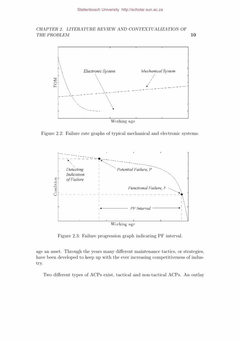
A typical example is that of a mechanical system where the failure rate in-creases with time due to the fact that failure in mechanical systems are most oftenage related. Another example is that of an electronic system. Electronic systemsexperience a higher failure rate in the beginning of its lifetime where after it staysconstant. Figure 2.1 illustrates these two concepts.
The second type of graphs, failure progression graphs, plot asset condition overworking age of the asset. A typical failure progression graph is shown in Figure2.3. Two points are defined on this graph, Potential failure, P, and Functionalfailure, F. This is known as the PF interval. Point P indicates where indicationsof failure start to appear. As time increases after point P, maintenance actionhas to be taken prior to point F. Point F indicates that a functional failure hasoccurred. From the graph it can be seen that point P acts as a trigger to initiatesome maintenance action before point F to avoid a functional failure.
The third ACP challenge, maintenance tactic selection, involves determiningwhat type of maintenance tactic should be chosen in an attempt to optimally man-
Stellenbosch University http://scholar.sun.ac.za
CHAPTER 2. LITERATURE REVIEW AND CONTEXTUALIZATION OFTHE PROBLEM 10
Figure 2.2: Failure rate graphs of typical mechanical and electronic systems.
Figure 2.3: Failure progression graph indicating PF interval.
age an asset. Through the years many different maintenance tactics, or strategies,have been developed to keep up with the ever increasing competitiveness of indus-try.
Two different types of ACPs exist, tactical and non-tactical ACPs. An outlay
Stellenbosch University http://scholar.sun.ac.za
CHAPTER 2. LITERATURE REVIEW AND CONTEXTUALIZATION OFTHE PROBLEM 11
of the following discussion is given in Figure 2.4.
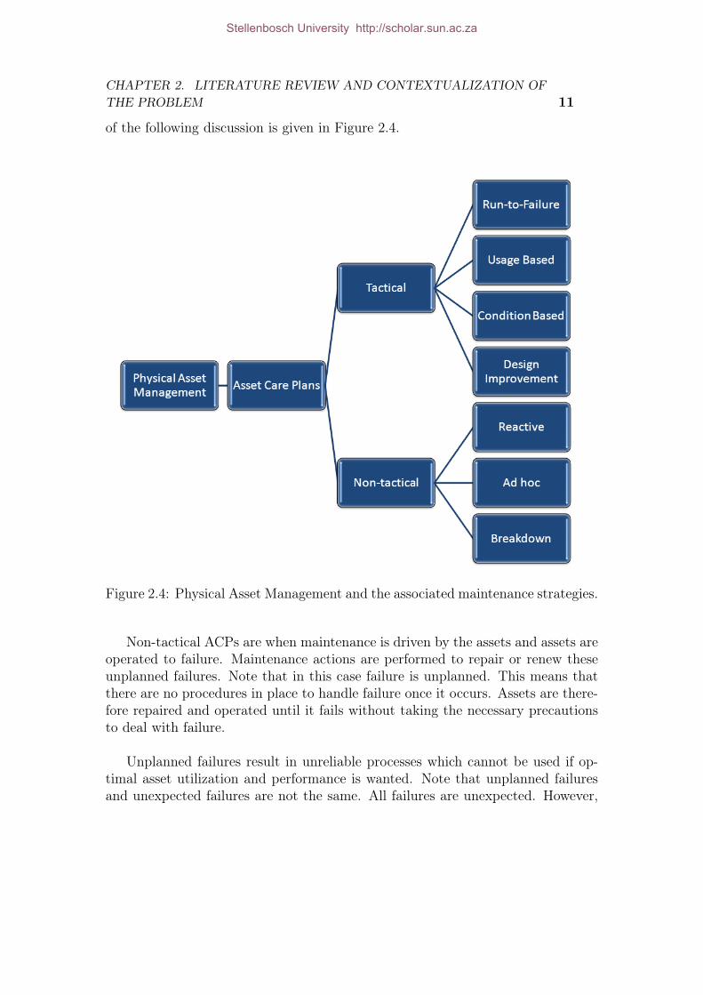
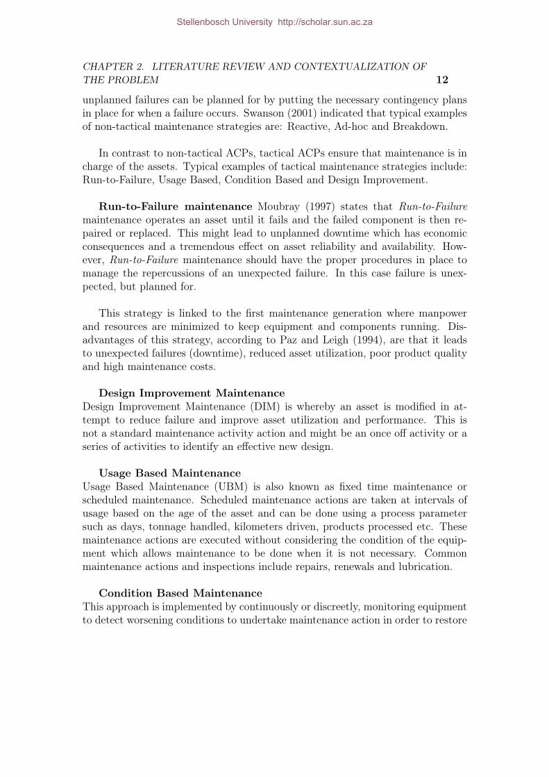
Figure 2.4: Physical Asset Management and the associated maintenance strategies.
Non-tactical ACPs are when maintenance is driven by the assets and assets areoperated to failure. Maintenance actions are performed to repair or renew theseunplanned failures. Note that in this case failure is unplanned. This means thatthere are no procedures in place to handle failure once it occurs. Assets are there-fore repaired and operated until it fails without taking the necessary precautionsto deal with failure.
Unplanned failures result in unreliable processes which cannot be used if op-timal asset utilization and performance is wanted. Note that unplanned failuresand unexpected failures are not the same. All failures are unexpected. However,
Stellenbosch University http://scholar.sun.ac.za
CHAPTER 2. LITERATURE REVIEW AND CONTEXTUALIZATION OFTHE PROBLEM 12
unplanned failures can be planned for by putting the necessary contingency plansin place for when a failure occurs. Swanson (2001) indicated that typical examplesof non-tactical maintenance strategies are: Reactive, Ad-hoc and Breakdown.
In contrast to non-tactical ACPs, tactical ACPs ensure that maintenance is incharge of the assets. Typical examples of tactical maintenance strategies include:Run-to-Failure, Usage Based, Condition Based and Design Improvement.
Run-to-Failure maintenance Moubray (1997) states that Run-to-Failuremaintenance operates an asset until it fails and the failed component is then re-paired or replaced. This might lead to unplanned downtime which has economicconsequences and a tremendous effect on asset reliability and availability. How-ever, Run-to-Failure maintenance should have the proper procedures in place tomanage the repercussions of an unexpected failure. In this case failure is unex-pected, but planned for.
This strategy is linked to the first maintenance generation where manpowerand resources are minimized to keep equipment and components running. Dis-advantages of this strategy, according to Paz and Leigh (1994), are that it leadsto unexpected failures (downtime), reduced asset utilization, poor product qualityand high maintenance costs.
Design Improvement MaintenanceDesign Improvement Maintenance (DIM) is whereby an asset is modified in at-tempt to reduce failure and improve asset utilization and performance. This isnot a standard maintenance activity action and might be an once off activity or aseries of activities to identify an effective new design.
Usage Based MaintenanceUsage Based Maintenance (UBM) is also known as fixed time maintenance orscheduled maintenance. Scheduled maintenance actions are taken at intervals ofusage based on the age of the asset and can be done using a process parametersuch as days, tonnage handled, kilometers driven, products processed etc. Thesemaintenance actions are executed without considering the condition of the equip-ment which allows maintenance to be done when it is not necessary. Commonmaintenance actions and inspections include repairs, renewals and lubrication.
Condition Based MaintenanceThis approach is implemented by continuously or discreetly, monitoring equipmentto detect worsening conditions to undertake maintenance action in order to restore
Stellenbosch University http://scholar.sun.ac.za
CHAPTER 2. LITERATURE REVIEW AND CONTEXTUALIZATION OFTHE PROBLEM 13
equipment to a "good-as-new" state before failure occurs. Maintenance action istaken when the health of the asset deteriorates to a predefined failure level. Per-forming maintenance in this manner is a preventive strategy which reduces theprobability of failure by taking preventive action before failure occurs. Delouxet al. (2009) argued that the advantage of this strategy is that maintenance ac-tions are only taken when it is imminent due to the fact that it is based on thephysical condition of the asset rather than fixed time intervals or failure.
It is therefore evident that of all the discussed maintenance strategies, CBMattempts to prevent failure whereas the other strategies only focusses on maintain-ing assets without taking the asset’s condition into account. Therefore, CBM hastremendous potential and is discussed in the Section 2.2.
Several authors such as Madu (2000), Nilsson and Bertling (2007), Wang et al.(2007), Endrenyi et al. (2001) and Márquez et al. (2009) indicate how the main-tenance strategies presented in this section can be applied in industry.
2.2 Condition Based MaintenanceAs mentioned, CBM utilize diagnostic equipment to monitor a condition of anasset and act only when maintenance is imminent before failure occurs. It ensuresthat maintenance action is taken as a preventive measure. An advantage of CBMis that it is possible to determine whether an asset can operate successfully duringa production period whereas an UBM strategy might indicate that a componentis due for replacement during the same production period.
Consequently, CBM is the preferred strategy due to the certainty it puts uponthe asset’s operational capability and the fact that the actual condition of theasset is taken into account. The idea of CBM is to ensure maintenance is doneonly when it is necessary resulting in a reduction in inventory levels and wastedmaintenance actions. Other advantages include an increase in reliability and areduction in the human error margin due to reduced maintenance operations.
It should however be noted that CBM can only give certainty about asset op-eration for a short period of time. Another major concern facing CBM is the costof implementation. Equipment used for CBM are extremely expensive to procureand install and does not guarantee any returns on this investment. Consequently acompany needs to evaluate the importance of an asset before implementing CBM
Stellenbosch University http://scholar.sun.ac.za

CHAPTER 2. LITERATURE REVIEW AND CONTEXTUALIZATION OFTHE PROBLEM 14
equipment.
Information extracted using CBM equipment is known as Condition Monitor-ing (CM) data. CM data is also known as explanatory variables or concomitantinformation. The CM data can be categorized into either quantitative or subjec-tive data. Quantitative data include measurements of (but are not limited to):temperature, tribology, vibration, pressure, oil content, stress, etc. Data may betime-dependent or time-independent and can either be measured continuously ormeasured at fixed process intervals.
Subjective data is known as indicator variables. This might include: whetheroil was changed at each service interval, what type of oil used, maintenance teamused, type of installation setup and supplier used. Subjective data might be foundon job cards which contain information such as who maintained, installed and sup-plied an item. For example, the inclusion of a subjective data provides the abilityto determine whether a maintenance team is associated with an event. It is thenpossible to track down some miscellaneous cause of a failure.
Subjective data can also be information such as job cards which contain infor-mation such as who maintained, installed and supplied an item. The inclusion ofa subjective covariate gives the ability to see whether it (absence of an oil change,certain maintenance team, supplier, setup, etc.) is associated with an event. Itis then possible to track down a possible cause of an event. With this data it ispossible to see whether neglecting maintenance contributes to the occurrence ofan event.
It would be ideal to obtain other subjective data by speaking with the technicalpersonnel that maintain and run the items. With their knowledge and experienceit might be easier to find subjective covariates which they believe contribute tothe occurrence of events.
Unfortunately the recording of CM data is done rigorously (and at great ex-pense) and rarely analyzed to enhance maintenance decision making. With accu-rate data it is possible to define a failure condition for a certain condition beingmeasured. Once the asset condition reaches this condition, maintenance actionshould be initiated to repair or renew the asset before failure occurs. In the casewhere only one condition is being measured, it is reasonably simple to define afailure condition.
Complex and expensive assets measure several different conditions to have as
Stellenbosch University http://scholar.sun.ac.za

CHAPTER 2. LITERATURE REVIEW AND CONTEXTUALIZATION OFTHE PROBLEM 15
much information about the health of the asset as possible. When several condi-tions are being measured, failure definition becomes extremely complex. Each ofthe conditions being measured might lead to failure but analysing one condition isnot adequate to prevent failure. Establishing a predefined failure condition whenseveral conditions are being measured is extremely complex due to the intricacyof identifying a correlation between the conditions being measured.
Other challenging factors such as environment and unforeseen- and random-failures increase the complexity of CBM. That being said, Heng et al. (2009) statedthat effective CBM implementation consists of three key elements.
(i.) Data Acquisition.
(ii.) Data Preparation.
(iii.) Decision Making: Development of asset management policies with informa-tion generated by processed asset data.
Each element is briefly discussed in the following sections.
2.2.1 Data Acquisition
Data acquisition in CBM is the collection and recording of useful asset data tobe used for maintenance decision making. A requirement of PAS55 is that anorganization shall design and maintain systems for managing asset managementinformation. Consequently, employees and relevant persons involved shall haveaccess to any asset information necessary to complete their tasks and activities.
Different methods exist to document this information and forms part of the In-formation Management KPA. Traditionally job-cards are used to document assetinformation but software such as Computerized Maintenance Management Sys-tem (CMMS) and Engineering Asset Management System (EAMS) can be usedto simplify this task. Software packages such as this has the capability of linkingall an assets’ information and storing it at on location. This property allows fordecreased data processing duration making data easily available for decision mak-ing. Another important capability of these software packages are that it can beused to generate and control work orders.
Asset data includes historical failure data and CM data. Historical failuredata contains the recorded time of failure and/or any preventive intervention suchas: preventative maintenance, scheduled maintenance and renewal. Any actiontaken which influenced the asset’s failure time is considered to be an event and
Stellenbosch University http://scholar.sun.ac.za

CHAPTER 2. LITERATURE REVIEW AND CONTEXTUALIZATION OFTHE PROBLEM 16
has to be documented in the historical failure data. The time scale used can beany convenient process parameter such as days, tonnage processed, liters pumped,kilometers driven, products processed, etc.
CM data, or concomitant information, can be categorized into quantitative andsubjective data. Concomitant information can also be recorded and stored usingCMMS software packages.
Jardine et al. (2006) discussed the fact that industry places more emphasison CM data than event data which leads to neglected and inaccurate event data.Event data and CM data both play crucial roles in effective CBM. A possiblereason why event data is being neglected and of bad quality, is that as supposeto CM data, which is recorded using diagnostic equipment, event data is enteredmanually. Manual entry of data has a high risk due to the human error involved.
2.2.2 Data Preparation
Data preparation is a process of extracting and selecting the most useful informa-tion contained in raw asset data. Data preparation basically entails data cleaning.Data cleaning is the removal of errors from a data set. Countless errors can befound in recorded event data and CM data. Errors in event data might be dueto the high margin of human error involved. Typical examples of errors in CMdata include faulty equipment recordings, missing data and incorrect data labels.Data cleaning plays an important role in data preparation and further discussionis done in Chapter 4.
2.2.3 Decision Making
Certain forms of CBM analyze event data in conjunction with CM data. Henget al. (2009) states that these forms of CBM use event data and CM data to de-velop mathematical models to represent the failure (or fault) behaviour of an asset.Mathematical models representing the failure behaviour of assets can the be usedto predict the future condition of the asset. Decision making in CBM can eitherbe done with diagnostics or prognostics. These concepts are designed to improvedecision making related to maintenance in attempt to maximize asset utilizationand performance. Both these concepts require some form of data analysis andmodel building.
Stellenbosch University http://scholar.sun.ac.za

CHAPTER 2. LITERATURE REVIEW AND CONTEXTUALIZATION OFTHE PROBLEM 17
2.2.3.1 Diagnostics
According to Caesarendra et al. (2010), diagnostics is the measurement of an as-set’s condition to identify, detect and isolate a fault condition before failure occurs.Venkatasubramanian et al. (2003b) presented three diagnostic approaches whichare quantitative model-based, qualitative model-based and process history based.
Figure 2.5: Diagnostics and its elements.
Quantitative and Qualitative Model Based: Venkatasubramanian et al.(2003b) showed that the most popular quantitative model based methods are di-agnostic observers, parity relations and Kalman filters. Qualitative model basedapplications can be seen in Venkatasubramanian et al. (2003a). Quantitative andmodel based applications are given by Isermann (2005) and Zheng et al. (2006),respectively.
Process History Based: The first process history method is statistical based.A statistical analysis is used to focus on the development of a fault hypothesisby comparing the current system condition with the fault hypothesis, which isa predefined failure condition after which deciding whether a fault is present ornot. Ma and Li (1995) showed that bearings experience localized defects and thesedefects comprise two alternating zero mean Gaussian distributions with their own
Stellenbosch University http://scholar.sun.ac.za

CHAPTER 2. LITERATURE REVIEW AND CONTEXTUALIZATION OFTHE PROBLEM 18
respective variances. Each Gaussian distribution is known as a hypothesis. Byusing both variances and a likelihood ratio test, the localized defect is present ifthe likelihood is greater than a certain defined level.
Kim et al. (2001) did a study on an internal combustion engine’s air and fuelsystem. Two hypothesis were developed and thresholds were determined for eachhypothesis respectively and then compared to measured values. The thresholdswere used to minimize the probability of incorrect fault detection and as an alarm.If the threshold criteria was met, a fault was present.
The second process history method is artificial intelligence based. Sorsa et al.(1991) showed that neural networks could be used to mimic human knowledge andpattern recognition ability. Another popular technique discussed by Mechefske(1998) was Fuzzy logic. The study was done using bearing frequency data anddifferent fuzzy logic membership curves were applied to find best fault classificationmethod.
2.2.3.2 Prognostics
Prognostics is used to predict when failures and/or faults may occur and to es-timate the remaining time left before these failures and/or faults occur. Theadvantage of knowing when faults and/or failures occur equips maintenance teamswith the knowledge to reduce maintenance costs, improve asset utilization andperformance by developing accurate maintenance schedules.
Prognostics focusses on two main outcomes. The first outcome is to determinehow much time is left before failure and/or fault(s) occur. This is referred to asthe Residual Useful Life (RUL) of an asset. The second outcome is the expectedtime until the next failure and/or fault(s) occur. This concept can be referred toas the Residual Useful Life Expected (RULE) of an asset.
Both RUL and RULE base their estimations on the given CM data and his-torical failure data. Statistical regression models are suitable for the combinedanalysis of historical failure data and CM data to determine these estimations.These time-dependent regression models can find a relation between the failureprobability using both the historical failure data and CM data. These modelsenable the prediction of future asset condition at a specified time in the futureenabling the estimation of RUL and RULE.
Stellenbosch University http://scholar.sun.ac.za
CHAPTER 2. LITERATURE REVIEW AND CONTEXTUALIZATION OFTHE PROBLEM 19
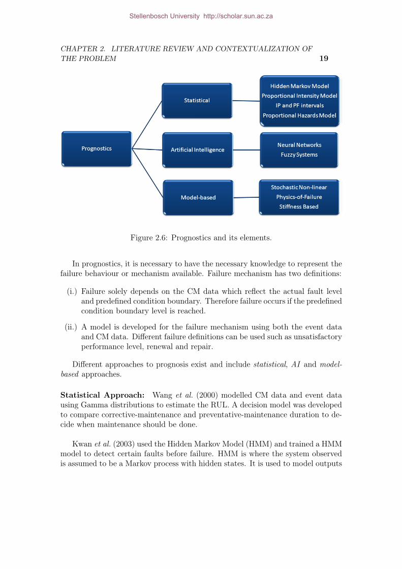
Figure 2.6: Prognostics and its elements.
In prognostics, it is necessary to have the necessary knowledge to represent thefailure behaviour or mechanism available. Failure mechanism has two definitions:
(i.) Failure solely depends on the CM data which reflect the actual fault leveland predefined condition boundary. Therefore failure occurs if the predefinedcondition boundary level is reached.
(ii.) A model is developed for the failure mechanism using both the event dataand CM data. Different failure definitions can be used such as unsatisfactoryperformance level, renewal and repair.
Different approaches to prognosis exist and include statistical, AI and model-based approaches.
Statistical Approach: Wang et al. (2000) modelled CM data and event datausing Gamma distributions to estimate the RUL. A decision model was developedto compare corrective-maintenance and preventative-maintenance duration to de-cide when maintenance should be done.
Kwan et al. (2003) used the Hidden Markov Model (HMM) and trained a HMMmodel to detect certain faults before failure. HMM is where the system observedis assumed to be a Markov process with hidden states. It is used to model outputs
Stellenbosch University http://scholar.sun.ac.za

CHAPTER 2. LITERATURE REVIEW AND CONTEXTUALIZATION OFTHE PROBLEM 20
that are generated by a finite number of states. The states are hidden (not visible),the the outputs can be measured. With the knowledge of the outputs it is possibleto determine the hidden states of the system.
Chinnam and Baruah (2003) showed how HMM clustering methods can be usedto facilitate autonomous prognostics by capturing the transition health states ofeach stage of the failure process by fitting a Gaussian distribution and estimatingthe RUL. Wang (2007) indicated how CM data can be used to identify the twostages of a components life, normal operating stage and failure delay stage. Thiswas done by modelling the unobserved state transitions using a HMM and com-paring results by fitting Weibull and Gamma distributions.
Goode et al. (2000) indicated how machine life can be separated into two inter-vals: IP (Installation Potential) interval in which the machine is running withoutfaults and the PF (Potential Failure) in which the machine is operating with afault. Weibull distributions were assumed for the IP and PF interval respectivelyand failure prediction was derived for each interval and the RUL estimation wasdone.
Vlok et al. (2004) showed how the Proportional Intensity Model can be usedto estimate bearing RUL. You et al. (2010) showed how the Proportional HazardsModel (PHM) and a two-zone extension thereof can be used to estimate the RUL.Banjevic and Jardine (2006) discussed the estimation of RUL using the PHM inconjunction with a Markov failure time process. Both PIM and PHM are regressionmodels are frequently used for reliability applications.
AI Approaches: These approaches found in literature were neural networksand fuzzy systems. Neural networks are developed by algorithmic training andfuzzy systems utilize linguistics for future system condition prediction. Wang andVachtsevanos (2001) proposed a prognosis architecture using a wavelet neural net-work to estimate fault growth and RUL. Wang et al. (2007) used a fuzzy analytichierarchy process to compare and evaluate different maintenance strategies.
Wang et al. (2004) showed how fuzzy systems can be trained using neuralnetworks and to determine failure definitions thereof. Chinnam and Baruah (2004)showed how a neuro-fuzzy model can be used to determine reliability estimationfor individual components using expert linguistic opinion and empirical data.
Model-based Approach: Model-based approaches require dynamic and/or staticinformation of an asset to develop a mathematical model in order to estimate RUL.
Stellenbosch University http://scholar.sun.ac.za
CHAPTER 2. LITERATURE REVIEW AND CONTEXTUALIZATION OFTHE PROBLEM 21
Ray and Tangirala (1996) applied a non-linear stochastic fatigue crack dynamicmodel to on-line monitoring of accumulated degradation and current degradationrates. Li et al. (2000) developed a stochastic non-linear bearing fatigue defect-propagation model which was recursively applied without prior knowledge of thesystem. Kacprzynski et al. (2004) showed how physics-of-failure modelling fusedwith diagnostic information and could be utilized to enhance the accuracy of he-licopter gear RUL estimation.
The study by Qiu et al. (2002) was done to develop a stiffness-based prognosticsmodel based on dynamic on-line vibration analysis and accumulative degradationmechanics. The study indicated that bearing lifetime can be analyzed and pre-dicted by monitoring the change in dynamic system stiffness based on the on-linevibration measurements. Caesarendra et al. (2010) used a model in the developingstages utilizing Monte Carlo based techniques and is known as the Particle Filermethod. It was shown that it exhibits some potential in predicting trending datain non-linear systems.
2.2.3.3 Conclusion
Diagnostics and prognostics are both CBM approaches used to attempt to preventfailure. Diagnostics take into account CM data and tests whether a predefinedfailure condition is reached. If this condition is met, maintenance action is initi-ated. Prognostics combines both CM data and historical failure data to estimateasset future condition. A major drawback of diagnostics is that it can only takeinto account one condition to define the failure condition.
Consequently, diagnostics is limited by the fact that it cannot take into ac-count several asset conditions to detect failure. This leads to less accurate resultscompared to prognostics. Three prognostic approaches were discussed in Section2.2.3.2. Statistical approaches fit distributions to data and develop models to pre-dict RUL and RULE. AI approaches train algorithms how assets behave which arethen used to predict asset RUL and RULE. Model-based approaches model datausing existing physics models.
From what was found in literature, statistical approaches have widely been ap-plied in the field of reliability in many different industrial applications. Statisticalapproaches are extremely flexible and has many applications.
Stellenbosch University http://scholar.sun.ac.za

CHAPTER 2. LITERATURE REVIEW AND CONTEXTUALIZATION OFTHE PROBLEM 22
2.3 Failure data analysisFailure data analysis is the statistical analysis of item/system failure data andthe point of interest is the time until failure occurs. Time is a process parameterdefined on any convenient time-scale. This process parameter is defined from acertain known origin up to the occurrence of an event event. Therefore it is im-portant to define how event times are measured. Event arrival times are typicallymeasured as shown in Figure 2.7.
Figure 2.7: Failure time measurement (Adapted from Vlok (2001)).
In figure 2.7 Xi refers to the interarrival time between the (i − 1)th event andthe ith event where i = 1, 2, .., n. The interarrival event times are random variableswith X0 ≡ 0. This variable is also known as local time. The so called real variable,xi, is used to indicate the elapsed time following the most recent event.
Ti refers to time measured from 0 to the ith event time. This variable is referredto as the arrival time to the ith event.In most cases Xi are used to analyze non-repairable systems whereas Ti is used to analyze repairable systems. The overalltime scale t is known as global time.
As shown by Coetzee (1997), after the event time has been measured it is nec-essary to determine the system type. Two system types exist which are repairableand non-repairable. A repairable systems can be repaired or renewed to its fullpotential to perform its intended functions correctly without the replacement ofthe entire system.
Time between events in repairable systems are dependent and not from thesame distribution, which means that repairable systems failure data is dependentand not identically distributed. With non-repairable systems, maintenance actions
Stellenbosch University http://scholar.sun.ac.za
CHAPTER 2. LITERATURE REVIEW AND CONTEXTUALIZATION OFTHE PROBLEM 23
are used to renew an entire system when a failure occurs.
Renewal results in an entire system restoration to a new state. Failure dataobtained from non-repairable systems are independent and identically distributed(i.i.d). After a system has failed and action is taken to repair it, it is in one of thefollowing states:
(i.) As good as new (GAN): A perfect repair or renewal which restored a systemto a condition equivalent to a new system.
(ii.) As bad as old (BAO): When a minimal repair was done which restored thesystem to the same state just before the event.
(iii.) Better than old but worse than new (BOWN): A repair restoring the systemto a state better than just before the event but worst than a total renewal,basically a state between old and new.
(iv.) Worse than old (WO): A repair or renewal which restored a system to acondition worse than before the event.
Further discussion on these assumptions are done in Section 2.3.3. An im-portant point of interest is model type selection. Selecting the most appropriatemodel to represent the failure behaviour of asset data is often neglected. Thereforea thorough discussion on this topic is done in the following section.
2.3.1 Model type selection
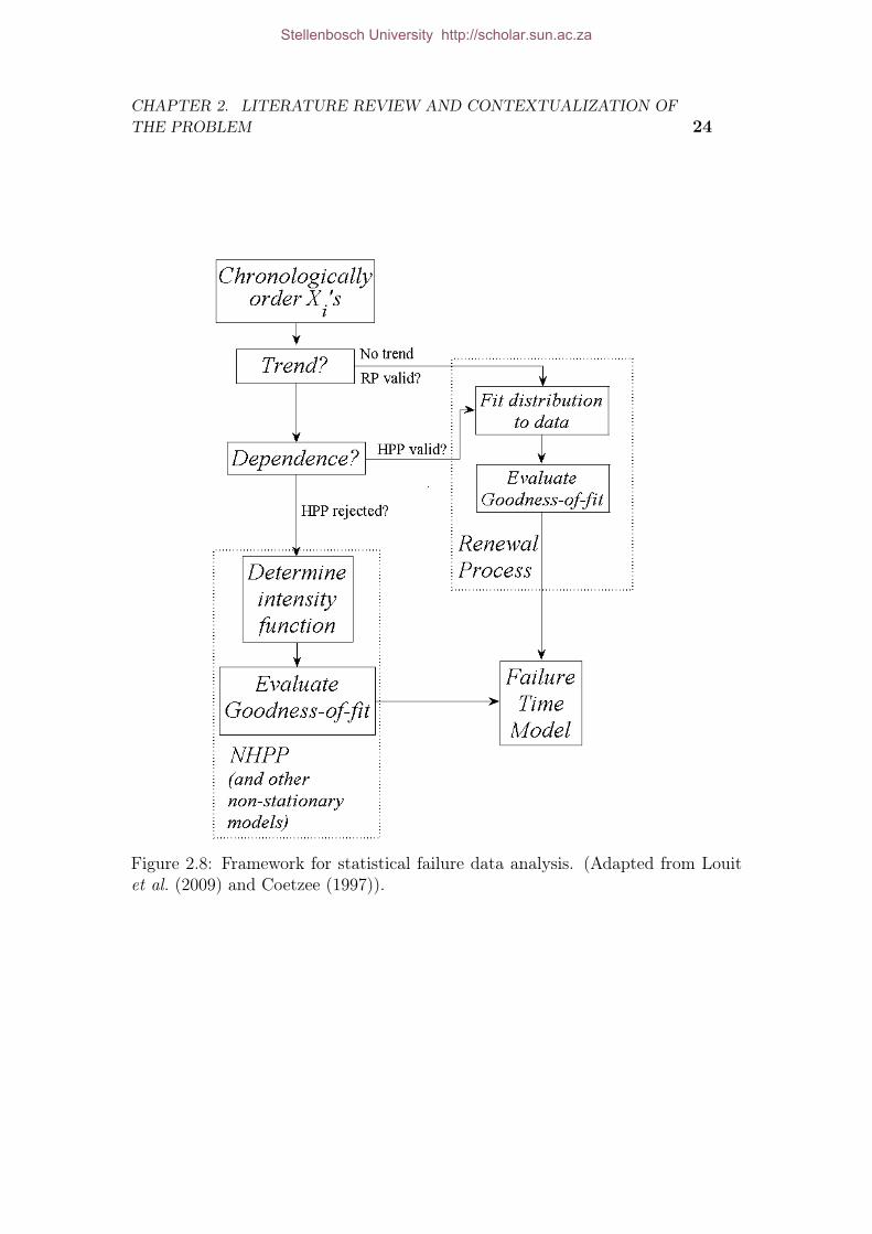
To model failure data, it is necessary to follow a selection process to determinewhich model fits the selected data best. It was found that most failure data analysisapplications do not pay much attention the model type selection process. Ascherand Feingold (1984b) set out a model selecting procedure using various trend testsand dependency tests. Coetzee (1997) and Louit et al. (2009) modified this pro-cedure mainly focussing on homogeneous- and non-homogeneous poison processmodels.
Their procedure was also modified and the resulting failure data model typeselection framework can be seen in figure 2.8. The main focus of this framework ison the Non-homogeneous Poison Process (NHPP) and the Renewal Process (RP).With that said, the framework helps to identify the failure process of the systembeing looked at. The two failure systems include a non-repairable system, RP, andrepairable systems.
Stellenbosch University http://scholar.sun.ac.za
CHAPTER 2. LITERATURE REVIEW AND CONTEXTUALIZATION OFTHE PROBLEM 24
Figure 2.8: Framework for statistical failure data analysis. (Adapted from Louitet al. (2009) and Coetzee (1997)).
Stellenbosch University http://scholar.sun.ac.za

CHAPTER 2. LITERATURE REVIEW AND CONTEXTUALIZATION OFTHE PROBLEM 25
(i.) Chronologically order X ′is: The first step in this process is to order the events
in their chronological order. Chronologically ordering the events is done torecognize trends in the data.
(ii.) Trend tests : Many techniques exist for trend testing. These tests basicallytests the renewal assumption. If a trend is present in the data, the renewalassumption is validated and the events are independent and identically dis-tributed. In testing for a trend, the objective is to determine whether aNHPP or Homogeneous Poison Process (HPP) model is applicable to use.Kvaloy and Lindqvist (1998) states that when testing for a trend special careshould be taken when selecting a time scale. The selection of the time scalemay have an effect on the occurrence of the event pattern. A trend in failuredata can be monotonic or non-monotonic.
Louit et al. (2009) states that monotonic trends can either be a "happy-system" or a "sad-system". A "happy-system" trend exists when the timebetween the events increase with increase in time. Thus as time increases,the trend decreases. A "Sad-system" trend exists when an increase in failureoccurs as time increases. In this case the trend increases as time increases.
Non-monotonic trends follow the bathtub curve and are therefore time de-pendent. Thus time between failures decrease in the beginning, then staysconstant and decreases near the end. A common graphical technique usedfor trend testing is the Total Time on Test (TTT) plot.
Analytical trend testing techniques include: Laplace test, Lewis-Robinsontest, Anderson-Darling trend test and Military handbook test. The Laplacetrend test was developed by Laplace (1773) and application of these graph-ical and analytical methods can be seen in Kvaloy and Lindqvist (1998).However, only the Laplace and Military handbook tests have a HPP nullhypothesis. This means that if no trend is found in the data, an HPP canbe applied because the data is i.i.d. If however a trend is found in the data,the data is assumed not to be i.i.d. and a NHPP can be used.
(iii.) Dependence Tests: The test for dependence is done to test for dependencybetween failure times without a long term trend. Coetzee (1997) suggeststhat any serial dependency test is adequate and proposes a test presentedby Krishnaiah and Sen (1984).
Stellenbosch University http://scholar.sun.ac.za

CHAPTER 2. LITERATURE REVIEW AND CONTEXTUALIZATION OFTHE PROBLEM 26
(iv.) Renewal Process: If the process leads to the RP, the failure data is i.i.d. andtherefore generated by a renewal process. Modelling this data is done byfitting a suitable statistical distribution to the data.
2.3.2 Censored data
Data is censored when an asset being monitored is taken out of service or is stilloperating correctly when the end of the measured interval is reached. According toMartinussen and Scheike (2006), right censoring is when an asset operated accept-ably for longer than the observed right censoring value or otherwise, the measuredinterval.
Right-censored failure data can however be used to estimate the regressionparameters that relate to the failure behaviour of the asset under study. However,if the censored data is not taken into account, basing the statistical analysis ononly the complete data would give bias results. Additionally, censored data cannotbe used in trend testing as it does not represent true failure times and could leadto erroneous results.
2.3.3 Reliability Theory
Reliability theory is focussed on estimating the probability or reliability of a certainitem based on historical failure data. Reliability is defined as the probability thatan item correctly performs its functions when installed in its intended applicationat time x.
Reliability=P(No failure at time x)
Note, Nachlas (2005) showed that it is possible to model stochastic survivaltimes of identical devices with probability and hence by a cumulative density dis-tribution. This distribution is the basis of four important descriptions of reliability.
(i.) Probability density function, f, which is the probability that an item that hasnot failed in the interval (0, x) fails in the interval (x, x+ δx).
(ii.) Cumulative failure distribution or Survivor function, F, which is the proba-bility that an item fails in the interval (0, x).
(iii.) Reliability function, R, which is the probability that an item does not fail inthe interval (0, x).
(iv.) Force of mortality is the instantaneous failure rate of an item that is workingcorrectly at time x in the interval (x, x+ δx).
Stellenbosch University http://scholar.sun.ac.za

CHAPTER 2. LITERATURE REVIEW AND CONTEXTUALIZATION OFTHE PROBLEM 27
These functions form the base of reliability engineering and are all related insome way in that if one function is known, it is possible to derive the other three.To illustrate this, the four functions is briefly discussed below.
2.3.3.1 Probability Density Function
The probability density function, f(x), represents the probability that an itemthat has not failed in the interval (0, x) fails in the interval (x, x+ δx) at time X.It is given that:
f(x)dx = P (x ≤ X < x+ δx) (2.3.1)
with f(x) ≥ 0 and the area under the probability density curve equal to unity,∞∫0
f(x)dx = 1.
2.3.3.2 Cumulative Failure Distribution
The cumulative density distribution, F (x), is the probability of a failure occur-ring before x, F (x) = P (X ≤ x). This probability can be obtained using theaccompanying probability density function and is given by:
F (x) =
x∫
0
f(x)dx (2.3.2)
As x tends to infinity, F (x) tends to unity.
2.3.3.3 Reliability Function
The reliability function is complimentary to the cumulative failure distributionand is also known as the survivor function. The reliability function, R(x), is theprobability that an item survives up to x, R(x) = P (X ≥ x). The reliabilityfunction is given by:
R(x) =
∫ ∞
x
f(x)dx (2.3.3)
where R(x) = 1− F (x). As x tends to infinity, R(x) tends to zero.
Stellenbosch University http://scholar.sun.ac.za

CHAPTER 2. LITERATURE REVIEW AND CONTEXTUALIZATION OFTHE PROBLEM 28
2.3.3.4 Force of Mortality
The force of mortality (FOM), h(x), is the statistical characteristic often used inreliability studies. The probability that an item might fail in the interval (x, x+δx),given that it is working correctly at time x, is known as a conditional probability.To define conditional probability, suppose there are two events, A and B, whereevent A is dependent on event B. The conditional probability of event A givenevent B is given by:
P (A|B) =P (A ∩ B)
P (B)(2.3.4)
where A ∩ B indicates that both event A and B take place and is valid ifP (B) &= 0. This implies that the conditional probability of event A given event Bis the probability that event A and B occurs divided by the probability that eventB occurs. Suppose h(x) represents the FOM and h(x)dx the probability that theitem is in a failed state at time X < x + dx given that no failure occurred atX = x. Therefore, by the definition of conditional provability, the FOM can begiven by:
h(x)dx = P (X < x+ δx|X > x) =P (X < x+ δx) ∩ P (X > x)
P (X > x)(2.3.5)
The numerator indicates the probability that an item might fail in the interval(x, x+δx) given that no failure occurred at X = x which is the probability densityfunction, f(t). The denominator indicates the probability that an failure mightnot occur in the interval (0, x) which is the reliability function, R(x). It can thenbe shown that Equation 4.6.5 can be given by:
h(x) =f(x)
R(x)(2.3.6)
Additionally, it is possible to determine the reliability function with the follow-ing relation:
R(x) = exp
−x∫
o
h(x)dx
(2.3.7)
The FOM is frequently used to describe the failure behaviour of an item. Inmany practical applications the FOM of similar complex items follow the bathtub
Stellenbosch University http://scholar.sun.ac.za

CHAPTER 2. LITERATURE REVIEW AND CONTEXTUALIZATION OFTHE PROBLEM 29
Figure 2.9: Graphical illustration of GAN assumption.
curve. As shown in Figure 2.1, the bathtub curve has three phases. Infant mor-tality, useful working life and wear-out.
A major concern to maintenance planners is which maintenance strategy toadopt in each of these three phases. When Equation 2.3.6 produces a constantrisk, failure is a random occurrence due to a constant failure probability. Forconstant failure probability items, the run-to-failure maintenance strategy can beused. For a decreasing FOM, the run-to-failure maintenance strategy should alsobe used due to the fact that the failure probability is decreasing.
However, if Equation 2.3.6 produces an increasing risk, the probability of failureincreases with an increase in time. Preventative maintenance has to be considered.An increasing FOM corresponds to the wear-out phase and a preventative main-tenance strategy such as CBM definitely has to be considered.
After a maintenance strategy has been selected, it is necessary to define thestate of the system after maintenance has taken place. From Section 2.3.1 it waspossible to determine whether the observed system is non-repairable or repairable.Knowing the system type presents the state of the system after a renewal or repair.Non-repairable systems are in a GAN state after each renewal. This assumptionimplies that the FOM is zeroed after each renewal. The GAN assumption is illus-trated in Figure 2.9.
Stellenbosch University http://scholar.sun.ac.za

CHAPTER 2. LITERATURE REVIEW AND CONTEXTUALIZATION OFTHE PROBLEM 30
Figure 2.10: Graphical illustration of BAO assumption.
Repairable systems is in a BAO state after a repair. With repairable systemmodelling it is assumed that simultaneous failures cannot occur. It should be notedthat the FOM is not used with repairable systems, but rather Rate of OCcurrenceOf Failure (ROCOF). ROCOF is defined as:
ROCOF =d
dtE {N(t)} (2.3.8)
where N(t) is the observed number of failures in (0, t]. Repairable systems canundergo degradation combined with an increased ROCOF causing a worseningtrend or even complete renewal of a system. Figure 2.10 is given to illustrate theBAO assumption.
Next we refer back to the wear-out phase of the bathtub curve. When a non-repairable system reaches the wear-out phase, a renewal brings the system backto a GAN state which means that the failure probability is zeroed. Consequently,non-repairable systems can be operated due the state after renewal. However,repairable systems which are repaired in the wear-out phase might experience anincrease in failure probability. Renewal therefore has no effect on the system fail-ure probability and system should be renewed to decrease the occurrence of failure.
Estimating the four reliability functions can be done using the statistical ap-proaches discussed in Section 2.2.3.2. The reliability functions is used to predict
Stellenbosch University http://scholar.sun.ac.za
CHAPTER 2. LITERATURE REVIEW AND CONTEXTUALIZATION OFTHE PROBLEM 31
asset RUL and RULE. It is possible to use these statistical approaches to modelrepairable and non-repairable systems.
The only approach looked at in this thesis is regression modelling. This ap-proach is frequently used in failure data analysis due to the fact that it is possibleto include time continuous explanatory variables, also known as regressors, or CMdata. Regression modelling is a statistical method and is part of prognostics.
Improved asset management can be done by implementing one or more KPAsuch as ACP development. These ACPs attempt to improve asset utilization andperformance through optimized maintenance activities such. Optimizing main-tenance can be done by using different types of maintenance strategies. It wasshown that some maintenance strategies, such as CBM, poses asset future con-dition modelling. Prediction of asset future condition is crucial to improve assetmanagement. Most traditional reliability modelling procedures only incorporatehistorical failure data. On the other hand, most maintenance strategies only takeinto account CM data.
CM data change stochastically and may influence and/or indicate the survivaltime of an asset. Omitting CM data might lead models which does not have theability accurately predict asset future condition resulting in the occurrence of fail-ure. Therefore, a need exists to model both event data and CM data together.Balakrishnan and Rao (2004) stated that models capable of this are known asregression models.
2.3.4 Regression Modelling
Many different regression models can be found in literature. It should howeverbe noted that a number of fundamental regression models exist upon which manyvariances thereof are based. These fundamental models are modified to suite theneeds of particular applications. Selection of regression model to research in thisthesis are evaluated according to the following criterion:
1. Previous application in the reliability engineering
2. Model originality
Six regression models were identified namely; Proportion Odds Model, AdditiveHazards Model, Proportional Hazards Model, Accelerated Failure Time Model,Proportional Intensity model and Extended Hazard Regression Model. Furtherdiscussion of these models are done in Chapter 3.
Stellenbosch University http://scholar.sun.ac.za

CHAPTER 2. LITERATURE REVIEW AND CONTEXTUALIZATION OFTHE PROBLEM 32
2.4 ConclusionThis chapter attempted to summarize the first item of the research methodol-ogy. PAM and ACP development was introduced where after several maintenancestrategies were looked at. It was found that CBM is the most suitable maintenancestrategy to achieve the objectives of this study. Further research of CBM indicatedthat a sub-field thereof is prognostics which is used for RUL predictions.
In order to determine these estimations, a school of thought called failure dataanalysis was presented. This lead to the identification of six suitable regressionmodels for this study. In Chapter 2 these regression models are evaluated accordingto the objectives of this research study.
Stellenbosch University http://scholar.sun.ac.za

Chapter 3
Regression models
3.1 IntroductionThe purpose of Chapter 3 is to evaluate the regression models identified in Chapter2 according to the thesis objectives. The most appropriate model is then selectedto accomplish the desired objectives of this thesis.
The six regression models identified in Chapter 2 were: Proportional Odds,Additive Hazards, Proportional Hazards, Accelerated Failure Time, ProportionalIntensity and Extended Hazard Regression. These models were identified basedon the criterion given in Chapter 2 which is repeated here for convenience.
1. Application in the field of reliability
2. Model originality
Several models were evaluated according to these criteria whereby six modelswere identified with the potential to achieve the thesis objectives. Many variationsof the six model can be found in literature each being modified for its specific ap-plication. A decision was then made to focus on the original six models uponwhich the variances are based upon.
The methodology of Chapter 3 is to evaluate the identified regression modelsaccording to the objectives of this thesis. After each model has been evaluatedthey are compared whereby the most suitable model is chosen.
Due to the mathematical content in this chapter, a number of mathematicalconcepts have to be defined. Note that it is assumed that an “event" and a “failure"have the same meaning and can interchangeably be used. Now, consider failure
33
Stellenbosch University http://scholar.sun.ac.za

CHAPTER 3. REGRESSION MODELS 34
Table 3.1: Regression model evaluation matrix.
Criteria WeightFuture potential 21
Implementation intricacy 22
Reliability application 23
Flexibility 24
time X > 0 and a vector of m covariates z(x) = [z1(x), z2(x), z3(x), ..., zm(x)] hasbeen observed. Each z(x) represents an asset condition as a function of time. Forgenerality, assume that covariates are time-dependent even though covariates canbe time-independent. Consequently, it is also assumed that the process parameterused in this chapter is time.
Furthermore, to incorporate the influence of covariates, a regression coefficientis associated with each of the m covariate vectors. Consider a row vector, γ, ofm regression coefficients i.e., γ = [γ1, γ2, γ3, ..., γm]. Estimation of these regressioncoefficients are done through model fitting procedures described in Chapter 4.
In this chapter the most suitable model for the thesis is determined. Eachmodel is presented mathematically and graphically followed by its advantages anddisadvantages. At the end of each section, the model is evaluated using the eval-uation criterion given in Table 3.1 followed by a brief description of each criteria.
Future potential evaluates possible future-use of the model in the field of re-liability. Reliability application identifies previous applications of the model inreliability. Implementation intricacy looks at the complexity of implementing themodel and the associated procedures involved. Flexibility is used to determine theextent to which the thesis objectives can be met with the particular model.
Each model is given a mark out of five for the respective criteria. To scalethe importance of the criterion, a weight is given to each criteria as shown in thesecond column of Table 3.1. In the final section of this chapter, a summarizingtable is given containing all the marks given to each model. This table also containsthe total mark of each model thereby indicating the most suitable model for thisthesis.
Stellenbosch University http://scholar.sun.ac.za

CHAPTER 3. REGRESSION MODELS 35
3.2 Proportional Odds ModelsThe Proportional Odds Model (POM) was introduced by McCullagh (1980) toanalyze failure times in the field of biomedicine. Bennett (1983a) first describedthe model in a semi-parametric framework and was further developed by severalauthors such as Yang and Prentice (1999).
In the POM, covariates act multiplicatively on the odds against failure time.Therefore, the odds of failure changes when covariate values change. However, astime increases the influence of the covariates diminish. Consider three FOM func-tions h1(x, z1), h2(x, z2) and h3(x, z3), where each FOM function is influenced by adifferent covariate. Figure 3.1 indicates how these functions converge illustratinghow the influence of covariates diminish over time.
Figure 3.1: Graphical illustration of how the covariate influence diminish overtime.
A typical example of systems where the influence of covariates diminish overtime are electronic systems. In Chapter 2 it was shown that electronic system oftenexperience decreasing probability of failure during infant mortality and convergeas time increases. Consequently, failure is a random occurrence and cannot becorrelated to the influence of the covariates. Due to this property, the POM hasnot seen much application in the field of reliability as reactive based maintenanceis applied where systems are experiencing random failure patterns. The odds of
Stellenbosch University http://scholar.sun.ac.za

CHAPTER 3. REGRESSION MODELS 36
an individual failing at time x is defined as:
FX(x)
RX(x)=
1−RX(x)
RX(x)(3.2.1)
However, by including covariates in Equation 3.2.1, the POM can be given by:
1−R(x, z(x))
R(x, z(x)= ψ · 1−RX(x)
RX(x)(3.2.2)
where ψ is a factor representing the multiplicative effect covariates have on theodds of failure. For instance, if ψ increases, the probability of failure is greaterwhich results in a shorter failure time. It should however be noted, covariate in-clusion does not necessarily result in a greater ψ value. Covariates can increase ordecrease the ψ value.
A commmon form of ψ given by Lu and Zhang (2007) is ψ = exp(z(x) · γ).Furthermore, Yang and Prentice (1999) states that if X is absolutely continuous,the FOM can be given by:
h(x, z) =1
ψ +RX(x)· dRX(x)
dx(3.2.3)
where RX(x) = F (x)/(1 − F (x)). Note that for any two covariates z1(x) andz2(x), h1(x; z)/h2(x; z) tend to unity with increase in x due to the covariate di-minishing property.
Bennett (1983b) proposed a profile likelihood method for model parameter es-timation. Profile likelihood, also known as full likelihood, estimates the unknownbaseline FOM function and the regression coefficients. Murphy et al. (1997) ap-plied the profile likelihood method and presented its POM parameter estimationcapabilities. Parameter estimation can also be done using Maximum LikelihoodEstimation (MLE) but the profile likelihood method is much less time consuming.
When time-dependent covariates are included in the model, parameter estima-tion can be done without too much effort. It becomes slightly more complex andtime-consuming when time-dependent covariates are included. Another limitationof the POM is that that little inference has been done to include censored data inthe POM. Authors such as Murphy et al. (1997) and Cheng et al. (1995) addressedthis limitation and presented POMs with censored data.
Stellenbosch University http://scholar.sun.ac.za

CHAPTER 3. REGRESSION MODELS 37
POM Advantages
According to Kirmani and Gupta (2001), the POM is a useful model when theprobability of failure converges over time due the diminishing effect of covariateinfluence. Another advantage of the POM is that parameter estimation is not toocomplex when time-independent covariates are included in the model.
POM Disadvantages
Including time-dependent covariates increases the complexity and time consump-tion of parameter estimation. Also, little research has been done to include cen-sored data in the POM model severely limiting the model in reliability.
Evaluation
In Table 3.2 the POM is evaluated according to each criteria with accompanyingreasons for the given marks. Reasons presented are based on the content of themodel presentation.
Table 3.2: Proportional Odds Model evaluation.
Criteria Mark ReasonFuture potential 2 Limited potential in reliabilityImplementation intricacy 3 Time-dependent covariates complexityReliability application 3 Limited applicationFlexibility 3 Censored data modelling
3.3 Additive Hazards ModelPijnenburg (1991) introduced the Additive Hazards Model (AHM) by modellingthe reliability of the air conditioning systems in aircraft. The AHM can be givenby:
h(x, z) = h0(x) + α (3.3.1)
where h0(x) is the baseline FOM and ψ the functional term. Lin et al. (1998)indicated that α can be given by α = λ(z(x) · γ). The baseline FOM is only afunction of time and is not affected by including covariates with α. Due to the
Stellenbosch University http://scholar.sun.ac.za

CHAPTER 3. REGRESSION MODELS 38
fact that α is added to the baseline FOM, covariates have a additive effect ratherthan a multiplicative effect.
This property of the model enables α to be negative without necessarily result-ing in a negative FOM. Gorjian et al. (2010) indicated that another useful propertyof AHM is that it is capable of modelling scenarios where the FOM is not zero attime zero. Both these properties are illustrated in Figure 3.2 where it is assumedthat α > 0.
Figure 3.2: Graphical illustration of the AHM.
In Figure 3.2 the additive effect of the covariates are represented by αi. Itcan also be seen that the FOM does not start at zero due to the addition of α0
at time zero. Also, at each point of failure Xi, the FOM is seen to experience a‘jump’ in FOM function value due to the assumption that α > 0 and the addi-tive affect of Equation 3.3.1. This ‘jump’ in function value indicates that somesort of maintenance action has been taken which influenced the FOM of the system.
As in the case of Figure 3.2 where α > 0, the state of a system is in a WOstate after maintenance action took place. On the other hand, scenarios whereα = 0, maintenance action had no effect on the FOM i.e., BAO. If however α ≤ 0,the system experienced a decrease in FOM after maintenance action took placei.e., BOWN. Note that in Chapter 2 it was stated that this thesis focusses on
Stellenbosch University http://scholar.sun.ac.za

CHAPTER 3. REGRESSION MODELS 39
non-repairable systems which assumes that a system is in a GAN state after main-tenance action has taken place. A non-repairable system can also be in a GANstate after maintenance action has taken place. However, although the system isin a GAN state, the system might be exposed to a higher FOM.
Parameter estimation can be done using the MLE and has proved to be acomplex procedure. Pijnenburg (1991) confirmed this statement indicating theintricacy of the likelihood equation inference.
AHM Advantages
A key merit of the model is that it offers a non-zero FOM at time zero. Inmost situations the FOM won’t be zero at time zero which renders this an usefulproperty.
AHM Disadvantages
As mentioned by Lin et al. (1998), a limitation of the AHM is that a negativefunctional term is allowed. The result is a negative FOM estimate which is anunrealistic and unreasonable assumption.
Evaluation
Table 3.3 contains the evaluation of the AHM according to each criteria with anaccompanying reason.
Table 3.3: Additive Hazards Model evaluation.
Criteria Mark ReasonFuture potential 3 Good potential for repairable systemsImplementation intricacy 4 Popular estimation methods are usedReliability application 4 Frequently applied in reliabilityFlexibility 3 Limited non-repairable system applications
3.4 Proportional Hazards ModelAccording to Orbe et al. (2002), the Proportional Hazards Model (PHM) is themost commonly used model in failure data analysis. The PHM was developed byCox (1972a) initially intended for the biomedical industry. Due to the success ofthe model in the biomedical industry, authors such as Ascher and Feingold (1984a)
Stellenbosch University http://scholar.sun.ac.za

CHAPTER 3. REGRESSION MODELS 40
and Dale (1985) decided to apply the model in the field of reliability. The origi-nal model developed by Cox (1972a) is a product of an arbitrary and unspecifiedbaseline FOM h0(x), and a functional term λ(z(x) ·γ). The FOM can be given by:
h(x, z) = h0(x) · λ(z(x) · γ) (3.4.1)
Before the discussion proceeds, it is necessary to define two assumptions of thePHM listed below.
1. Variables which affect the failure times of the items are included in the model.
2. For any two sets of time-independent sets of covariates, z1 and z2, for asingle item, their associated FOM values are proportional with respect totime. Note that this assumption only holds for time-independent covariates.
The first assumptions states that all the environmental influences affecting thefailure times of the item being studied are included in the model. Then, two setsof time-independent covariates are assumed to have proportional FOM functions.These two functions, h1(x, z) and h2(x, z), are also proportional to the baselineFOM h0(x). Figure 3.3 illustrates the proportional FOM assumption.
Figure 3.3: Graphical illustration of the proportional FOM assumption.
Stellenbosch University http://scholar.sun.ac.za

CHAPTER 3. REGRESSION MODELS 41
Furthermore, due to the construction of the model, covariates act multiplica-tively on the FOM. The functional term, λ(z(x)), can adopt several different forms.Some of these forms are: the logarithmic form, log(1 + exp(z(x) · γ)); the inverselinear form, 1/(1 + (z(x) · γ); the linear from, 1 + (z(x) · γ and the exponentialform, exp((z(x) · γ). In most reliability applications, the exponential form is usedwhereby Equation 4.1.1 can be given by:
h(x, z) = h0(x) · exp(z(x) · γ) (3.4.2)
Parameter estimation can be done using the Partial Likelihood Method (PLM)developed by Cox (1972a). Further developments of the model has indicated thatthe MLE can also be used to estimate the model parameters. Kalbfleisch andPrentice (1980) presents both the PLM and the MLE for the PHM.
A key advantage of this model is that no assumption has to be made aboutthe baseline FOM of Equation 4.1.1. That means that parameter estimation canbe done without having to make any assumption about the baseline FOM duringmodel fitting procedures. A common form of the baseline FOM found in literatureis the Weibull distribution. Substituting the Weibull distribution in Equation 3.4.2yields:
h(x, z) =β
η
(x
η
)β−1
· exp(z(x) · γ) (3.4.3)
where β and η are known as the shape and scale parameters respectively. Thisform of the PHM is known as the Weibull PHM and was presented by Jardineet al. (1987). Authors such as Ghasemi et al. (2009), Tian and Liao (2011) andWong et al. (2010) applied the Weibull PHM in the field of reliability.
Seetharaman and Chintagunta (2003) indicates that alternative parametric dis-tributions such as the inverse Gaussian, Erlang, Log-logistic, Exponential, Log-normal, Raleigh and Gompertz can be utilized for estimating the baseline FOM.
Another important property of the model is that it is possible to include cen-sored events in the data. This enables modelling of items which have been takenout of service before having reached failure. An example of such a situation iswhere an item’s dataset contains fewer failures than censored events. Such a studymight indicate that maintenance took place too early and could have been post-poned without encountering failure. Postponement might result in improved item
Stellenbosch University http://scholar.sun.ac.za

CHAPTER 3. REGRESSION MODELS 42
performance and utilization.
Furthermore, a limitation of the model however is that small sample sizesshould be avoided. Orbe et al. (2002) states that regression coefficients are biasedtowards certain covariates when small sample sizes are used.
PHM Advantages
The key merit of the PHM is that parameter estimation can be done without mak-ing an assumption about the baseline FOM. As with the POM model, covariatesact multiplicative on the FOM which is a more reasonable and realistic assumptioncompared to models such as the AHM. A common form of the baseline FOM isthe Weibull distribution. Application of this distribution is a special case of thePHM known as the Weibull PHM. The Weibull PHM is a flexible model and hasrepeatedly been applied in the field of reliability.
PHM Disadvantages
Using small sample sizes results in regression coefficients biased towards certaincovariates.
Evaluation
Table 3.4 contains the evaluation of the PHM according to each criteria with anaccompanying reason.
Table 3.4: Proportional Hazards Model evaluation.
Criteria Mark ReasonFuture potential 5 Good future in reliabilityImplementation intricacy 4 Popular estimation methods can be usedReliability application 5 High application frequency in reliabilityFlexibility 4 Weibull PHM exhibits good flexibility
3.5 Accelerated Failure Time ModelPike (1966) introduced the Accelerated Failure Time Model (AFTM). The AFTMis a parametric model which estimates the relation between the log expected fail-ure time and covariates in a familiar form of a linear regression equation. It allows
Stellenbosch University http://scholar.sun.ac.za

CHAPTER 3. REGRESSION MODELS 43
covariates to act multiplicatively on the failure time of an item.
Cheung et al. (2001) showed that it is intuitive to analyze the effects of co-variates using failure time ratios. In this section, the AFTM is presented in twoways. For the first representation, suppose that the AFTM estimates a log-linearregression lifetime Y = log(X). This is related to the covariate vector (x) via alinear model:
log(X) = z(x) · γ + ε (3.5.1)
where ε is a measure of variability in the failure times. Substituting γ and z(x)into Equation 3.5.1 yields:
log(X) = γ0 + z1 · γ1 + z2 · γ2 + ...+ zm · γm + ε. (3.5.2)
If the coefficients of the above equation are exponentiated, exp(γm), it is knownas the Time Ratio (TR). The TR can be used to estimate the failure time of anitem. A TR > 1 implies that the time-to-event slows down, in other words in-creasing the time-to-event. On the other hand, a TR < 1 indicates that a shorterfailure time is more likely. Therefore, covariates act multiplicatively on the failuretime rather than on the FOM. Figure 3.4 illustrates different TR values and itseffect of the failure probability time-scale of an item.
A common use of the AFTM is modelling electronic equipment to determinethe failure probability of an item at different temperature levels over a given periodof time. The AFTM also has repeatedly been applied in biomedical applicationsto model the effect different medication dosages may have.
The FOM of the AFTM can be written as:
h(x, z(x)) = λ(z(x)) · h0(z(x) · x) (3.5.3)
where h0(z(x) · x) is the baseline FOM.
For the second representation, suppose that the reliability function is givenby RX(x) and the accelerated reliability function by RX(x), resulting from stressor environmental influences. These influences are captured in covariate measure-ments. When covariates change it affects the model parameter values. Conse-quently, changes in covariates values results in time scale transformations of the
Stellenbosch University http://scholar.sun.ac.za

CHAPTER 3. REGRESSION MODELS 44
Figure 3.4: Different TR values and how it affects the failure probability time-scaleof an item.
FOM and the other reliability equations. This was confirmed by Newby (1988)doing a study on fatigue crack growth applying both the AFTM and the PHM.For the AFTM, each of the reliability functions are shown to be related by:
RX(x) = R[(x− c)/b] (3.5.4)
where b is a scale parameter and c a location parameter. The AFTM model issimilar to other regression models which assume that (x− c)/b has a distributionrelated to a known parametric form. This leads to the use of shape, scale andlocation parameter families of distributions. With these distributions the failuretimes do not change with the level of covariate influence but is rather acceleratedor decelerated.
Some probability density functions used in reliability analysis (which form partof the shape, scale an location families) are:
Weibull:fX(x) =
k
buk−1 exp(−uk), u = x/b (3.5.5)
Stellenbosch University http://scholar.sun.ac.za

CHAPTER 3. REGRESSION MODELS 45
Gamma:fX(x) =
1
bΓ(k)uk−1 exp(−u)], u = x/b (3.5.6)
Log-normal:
fX(x) =1
buk√2π
exp
{−1
2
[ln(u)
k
]2}uk−1 exp(−u)], u = (x− c)/b (3.5.7)
Inverse Gaussian:
fX(x) =1
b
√k
2πu−3/2 exp
{−−k(u− 1)2
2u
}, u = x/b (3.5.8)
where b and c are as defined and k a shape parameter. If it is possible to finda distribution which adequately describes the data, a new definition of the prob-ability density function is fX(x, k) with a corresponding AFTM density functionof fX((x/bi), k), where bi = b(z(x), q) and q a coefficient parameter.
Quasi-linear models are assumed to be in the form of b = k(z(x) · c) andb = k(z(x) · a). Other forms of b are:
1. Constant.
2. Linear function of stress, b = (z(x) · a).
3. Exponential function, bi = exp(zi · a).
4. Inverse exponential Arrhenius model, bi = exp(−1/(z(x) · a)).
Parameter estimation can be done using either the partial likelihood methoddeveloped by Cox (1972a) and the MLE. Supporting this statement is Newby(1988), Shyur et al. (1999), Shyur et al. (1999) and Orbe et al. (2002). Thesemethods are often used in literature which reduces the implementation complexitythereof. Qi (2009) used this method by maximizing the log-likelihood function toestimate the model parameters.
Application in the field of reliability has however been limited. A reason forthis might be that parameter estimation is done by assuming a distribution forthe failure times. Failure time distributions are intricate to identify and timeconsuming to determine. Another reason might be the fact that the inclusion ofcensored data has not seen much development.
Stellenbosch University http://scholar.sun.ac.za
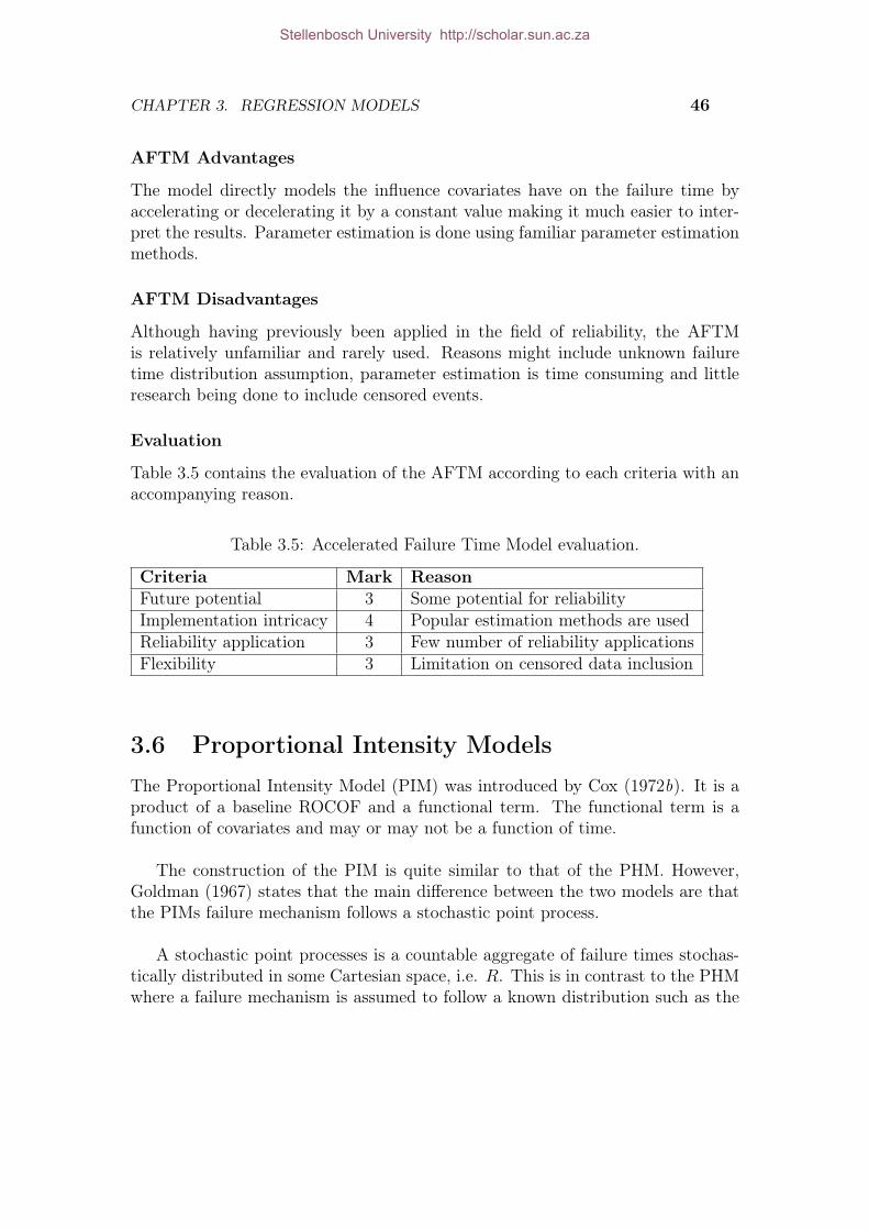
CHAPTER 3. REGRESSION MODELS 46
AFTM Advantages
The model directly models the influence covariates have on the failure time byaccelerating or decelerating it by a constant value making it much easier to inter-pret the results. Parameter estimation is done using familiar parameter estimationmethods.
AFTM Disadvantages
Although having previously been applied in the field of reliability, the AFTMis relatively unfamiliar and rarely used. Reasons might include unknown failuretime distribution assumption, parameter estimation is time consuming and littleresearch being done to include censored events.
Evaluation
Table 3.5 contains the evaluation of the AFTM according to each criteria with anaccompanying reason.
Table 3.5: Accelerated Failure Time Model evaluation.
Criteria Mark ReasonFuture potential 3 Some potential for reliabilityImplementation intricacy 4 Popular estimation methods are usedReliability application 3 Few number of reliability applicationsFlexibility 3 Limitation on censored data inclusion
3.6 Proportional Intensity ModelsThe Proportional Intensity Model (PIM) was introduced by Cox (1972b). It is aproduct of a baseline ROCOF and a functional term. The functional term is afunction of covariates and may or may not be a function of time.
The construction of the PIM is quite similar to that of the PHM. However,Goldman (1967) states that the main difference between the two models are thatthe PIMs failure mechanism follows a stochastic point process.
A stochastic point processes is a countable aggregate of failure times stochas-tically distributed in some Cartesian space, i.e. R. This is in contrast to the PHMwhere a failure mechanism is assumed to follow a known distribution such as the
Stellenbosch University http://scholar.sun.ac.za

CHAPTER 3. REGRESSION MODELS 47
Weibull distribution. As a result, it is often found that the PIM does not assumesystem renewal at failure.
Now, consider a baseline ROCOF ιU0(t), and the functional term λ(t, z(t)).The PIM model can then be given by:
ιU(t) = ιU0(t) · λ(z(t), t) (3.6.1)
Possible forms of the baseline ROCOF, ιU0(t), can be adopted. Three of theseforms are: power-law, αtβ; constant α and log-linear, αβt. A form adopted inthe field of reliability for the functional term, λ(t, z(t)), is given by exp(z(t), γ).Estimation of the γ parameters is done using the MLE. Due to the large amountunknown parameters, parameter estimation is a complex process.
Authors such as Love and Guo (1991), Percy and Alkali (2006), Jiang et al.(2006), Lugtigheid et al. (2007) and Percy and Alkali (2007) have illustrated howthe PIM can be implemented in the field of reliability.
PIM Advantages
Parameter estimation can be done without making any assumptions about thebaseline ROCOF. Also, the PIM does not assume that a system is renewed atfailure such as the PHM.
PIM Disadvantages
The PIM is limited to repairable systems due to the fact that it does not assumesystem renewal at failure. However, Vlok et al. (2004) introduced a variation ofthe PIM for both repairable and non-repairable systems. Lastly, the process ofparameter estimation is complex due to the large number of unknown parameters.
Evaluation
Table 3.6 contains the evaluation of the PIM according to each criteria with anaccompanying reason.
3.7 Extended Hazard Regression ModelThe Extended Hazard Regression Model (EHRM) was introduced by Ciampi andEtezadi-Amoli (1985) and Etezadi-Amoli and Ciampi (1987) and includes both thePHM and the AFTM. A general expression for the FOM is given by:
Stellenbosch University http://scholar.sun.ac.za

CHAPTER 3. REGRESSION MODELS 48
Table 3.6: Proportional Intensity Model evaluation.
Criteria Mark ReasonFuture potential 4 Good future potential for reliabilityImplementation intricacy 3 Complex parameter estimationReliability application 4 Often applied in reliabilityFlexibility 2 Some limitation to system type
h(x, z) = g1(z(x) · a) · h0[g2(z(x) · b) · x] (3.7.1)
Where a and b are regression coefficient vectors and g1(·) = g2(·) = 1 at timezero. When b = 0, Equation 3.7.1 reduces to the PHM and when a = b, Equation3.7.1 reduces to the AFTM. Therefore indicating the presence of properties of boththe PHM and AFTM in the EHRM. The multiplicative effect of the covariates onthe FOM of the PHM is interpreted by the b and the time-scale changing effect ofthe AFTM is interpreted by the a.
Estimation of the baseline FOM can be done using the method of quadraticsplines. A quadratic spline is a piecewise polynomial of n degrees with pieces join-ing at a number locations called knots, failure times. By illustration, Figure 3.5illustrates how quadratic splines can be used to join knots to estimate a baselineFOM.
It should however be noted, utilizing quadratic splines to estimate the baselineFOM does not ensure a positive FOM. For example, if the 5th failure in Figure 3.5were close to zero, the spline arc could have intercepted the y-axis resulting in anegative FOM.
Furthermore, application of the model is fairly complex due to the fact thatthe unknown parameters, β and η, have to be estimated simultaneously. Elsayedet al. (2006) sets out a method to estimate these parameters using the MLE butalso comments on the complexity involved.
EHRM Advantages
The MLE is used to estimate the unknown model parameters of the EHRM. Shyuret al. (1999) states that the EHRM is a useful regression model with the futurepotential in the field of reliability.
Stellenbosch University http://scholar.sun.ac.za

CHAPTER 3. REGRESSION MODELS 49
Figure 3.5: Baseline Foce Of Mortality estimation using quadratic splines.
EHRM Disadvantages
The EHRM has a major drawback where a positive FOM cannot be ensured placinga great deal of uncertainty in the model’s ability to model a reliability situationrealistically.
Evaluation
Table 3.7 contains the evaluation of the EHRM according to each criteria with anaccompanying reason.
Table 3.7: Extended Hazard Regression Model evaluation.
Criteria Mark ReasonFuture potential 2 Limited reliability applicationImplementation intricacy 2 Complex parameter estimationReliability application 3 Seldom applicationFlexibility 3 Baseline FOM estimation
Stellenbosch University http://scholar.sun.ac.za

CHAPTER 3. REGRESSION MODELS 50
3.8 Model SelectionIn Chapter 2 a primary selection process was done to identify models with the po-tential achieve the thesis objectives. In this chapter each of those selected modelswere presented and evaluated according to criterion given in Section 3.1.
Models were evaluated according to each criteria and given a mark out of five.In Table 3.8 each model’s total mark is calculated taking into account the weightsof the criterion.
Table 3.8: Selection of most suitable regression model.
Regression Model EvaluationCriterion Weight POM AHM PHM AFTM PIM EHRMFuture potential 21 2 3 5 3 4 2Reliability application 22 3 4 4 4 3 2Implementation intricacy 23 3 4 5 3 4 3Flexibility 24 3 3 4 3 2 3
Total Score: 31 98 126 90 81 82
This indicates that the PHM is the most suitable regression model for the the-sis. From this point forward, the sole focus of the thesis is on the PHM. Chapter4 provides an in-depth study of the PHM with a keen focus on the mathematicalmodel, parameter estimation, model fitting procedures and a decision model.
3.9 ConclusionThis chapter addressed the second item of the methodology whereby models iden-tified in Chapter 2 are evaluated according to four criterion reflecting the appli-cability of the model to achieve the objectives of this research project. The mostappropriate model was then selected based on these criterion and it was foundthat the PHM is the most suitable model for this thesis.
Stellenbosch University http://scholar.sun.ac.za

Chapter 4
Proportional Hazards Model
4.1 IntroductionSeveral regression models were evaluated in Chapter 3 of which the ProportionalHazard Model (PHM) was chosen as the most suitable model for this thesis. InChapter 4, the methodology is to perform a comprehensive study on the PHMfocussing on the mathematics and practical implementation thereof. The chapterconcludes with a brief look at some decision models which are used together withthe PHM to develop ACPs.
When the PHM was introduced by Cox (1972a), its initial intention was for itto be used for biomedical applications. After the success of the model in this field,several authors discovered that the PHM can be used in reliability applications.Consequently, an abundance of reliability applications can be found in literature.Some examples of where the model has been applied in reliability applications are:mining haul truck wheel motors (Jardine et al., 2001), circulating pumps (Vloket al., 2002), locomotive wheel set bearings (Feng et al., 2009), preventive main-tenance scheduling (Samrout et al., 2009), military vehicle diesel engines (Wonget al., 2010), electrical transformers (Wu and Ryan, 2011), solder joint’s life span(You et al., 2011) and semiconductor manufacturing (Pampuri et al., 2011).
These examples utilize different variations of the model to compensate for thespecific needs of each application. For this reason, it is not practical to discussevery variation of the model. The discussion is limited to the mathematical theorynecessary to apply the model in practical situations.
The PHM model is a product of an arbitrary and unspecified baseline FOMh0(x), and a functional term λ(x · z(x)). The functional term is a function of time
51
Stellenbosch University http://scholar.sun.ac.za

CHAPTER 4. PROPORTIONAL HAZARDS MODEL 52
and covariates. Note, if the covariates are independent of time, then the functionalterm is a function of covariates only, i.e. λ(z).
Let h(x, z) represent the FOM at time x with corresponding covariate vectorzi(x) = [z1, z2, z3, ..., zn]. For the sake of generality, theory presented in this thesisconsider time-dependent covariates. The FOM is therefore given as:
h(x, z(x)) = h0(x)λ(x · z(x)) (4.1.1)
In Chapter 3 it was indicated that several forms of the functional term areconsidered and that most reliability applications of the PHM adopt the exponentialform, i.e. exp(z(x), γ). Substituting this form of the functional term in Equation4.1.1 yields:
h(x, z(x)) = h0(x) exp(z(x) · γ) (4.1.2)
where γ is a row vector containing the regression coefficients. These coefficientsare estimated during model fitting procedures discussed in Section 4.5.
Two forms of the PHM are discussed in this thesis. The first form is thesemi-parametric form which does not make any assumptions about the baselineFOM. The second form fully specifies the baseline FOM and is known as the fully-parametric form. Then, an algorithm is discussed which was used for numericalmodel fitting procedures. And finally, decision models are introduced with whichimproved maintenance plans can be developed.
4.2 CensoringIn Chapter 2 censoring was briefly discussed where it was stated that censoringplays a crucial role in reliability analysis because it allows the inclusion of itemsin the model which have not yet failed. In order to determine model parameters,the likelihood function needs to be derived whereby it is necessary to consider thecensoring mechanism acting on the failure data.
Likelihood is the conditional probability that an item, which has already failed,yields a certain outcome. This is in contrast to probability which is based on eventsthat have not yet occurred.
Let n items be put on test where Xi indicates failure times and zi(x) cor-responding covariate vectors. A subjective variable, ci, is introduced indicating
Stellenbosch University http://scholar.sun.ac.za

CHAPTER 4. PROPORTIONAL HAZARDS MODEL 53
either an observed failure, ci = 1, or a censored observation, ci = 0. In thereliability field, three censoring types are observed:
1. Drop Out : The item fails in the duration of an experiment resulting in anuncensored observation.
2. Termination of Experiment : The item has not yet failed at the end of anexperiment resulting in a censored observation.
3. Follow-up: The item is lost during the duration of an experiment resultingin a censored observation.
Figure 4.1 illustrates three failure times to indicate each form of censoring.Thefirst item failed at time X1 resulting in an uncensored observation. Item numbertwo hadn’t failed at the end of the experiment resulting in a censored observationX+
2 . The third item was lost during the experiment which resulted in anothercensored observation X+
3 .
Figure 4.1: Three types of Random censoring.
Three mechanisms of censoring are discussed in this chapter, namely (a) ran-dom censoring, (b) type I censoring and (c) type II censoring.
Stellenbosch University http://scholar.sun.ac.za
CHAPTER 4. PROPORTIONAL HAZARDS MODEL 54
Random censoring
Let the time to censoring be Ci with probability density and survivor functionsgi(x) and Gi(x) respectively. Also Ci = C1, C2, C3, ..., Cn are randomly and inde-pendently distributed of each other and of the failure times Xi = [X1, X2, X3..., Xn].
It might seem confusing that Ci and Xi are similar. To clear up confusion, theith individual may or may not be observed due to censoring and therefore failuretimes, Xi, and censoring times, Ci, are not the same where censored observationsare found.
Using random censoring can be used to include type I censoring. Randomcensoring also allows items to enter the study at random instances. Kalbfleischand Prentice (1980) indicated that for random censorship the probability of failuretime Xi occurring in (x, x+ dx) is given by:
P[Xi ∈ (x, x+ dx), ci = 1; zi(x), γ
]= Gi(x+ 0)f(x; zi(x), γ)dt (4.2.1)
and
P[Xi ∈ (x, x+ dx), ci = 0; zi(x), γ
]= gi(x)F (x+ 0; zi(x), γ)dt (4.2.2)
where if F is continuous, F (x+ 0; zi(x), γ) = F (x; zi(x), γ).
Type I censoring
Here censoring times of an item is fixed at the start of an experiment wherby amaintenance eam knows exactly when maintenance is going to be performed on anitem. Typically this is a maintenance strategy such as Usage Based Maintenance.
If it is found that Gi(x) do not involve any parameters of interest, i.e. γ,Equations 4.2.1 and 4.2.2 simplify to:
L(γ) =n∏
i=1
[f(Xi; z(x); γ)
ci · F (Xi; z(x); γ)1−ci
](4.2.3)
which is the likelihood function for type I censoring. Some equations, such asEquation 4.2.3, are introduced in this section although their use shall become clearin sections to follow. It is the product of each item’s likelihood function given by:
L(γ) =∏
Li(γ) (4.2.4)
Stellenbosch University http://scholar.sun.ac.za
CHAPTER 4. PROPORTIONAL HAZARDS MODEL 55
where Li(γ) is f(Xi, z(x), γ) for a failure and F (Xi, z(x), γ) for a censoredobservation. Type I censoring can typically be found in Use Based Maintenance(UBM) situations.
Type II censoring
Type II censoring times are unknown at the beginning of an experiment. Censor-ing time is a function of the amount of items which has failed. Items are operateduntil r out of n items have failed. So the r shortest failure times are observed tofail and the remaining n− r items are censored.
Hence, data consist of the r shortest failure times and n− r censored observa-tions. The likelihood function can be given by:
L =n!
(n− r)!(f(X1) · · · f(Xr))(F (Xr))
n−r (4.2.5)
For example, if a plant requires r out of n pumps operational for acceptableand reliable operation, type II censoring can be used indicate when downtime isnecessary to perform maintenance in order to ensure that r pumps are available.
For both Type I and Type II censoring, the likelihood construction is thesame. In both cases items that fail contribute to the f(Xi) term and censoreditems contribute to the F (Xi) term.
4.3 Semi-parametric PHMThe main advantage of this form is that baseline FOM is left unspecified. Thismodel utilizes the FOM in Equation 4.1.2 with a functional term in the exponentialform, i.e. exp(z(x) · γ), which is given as:
exp(z(x) · γ) = exp
[k∑
m=1
zm(x) · γm
](4.3.1)
where k indicates the number of covariate measurements. From this it can beseen that the covariates are fully specified whereas the baseline FOM is unspeci-fied. For this reason the model is called the semi-parametric model.
Semi-parametric PHM regression coefficient inference can be done using amethod introduced by Cox (1972a) known as the method of partial likelihood. Asan introduction to this estimation method, likelihood and the Maximum LikelihoodEstimate are discussed.
Stellenbosch University http://scholar.sun.ac.za
CHAPTER 4. PROPORTIONAL HAZARDS MODEL 56
4.3.1 Maximum Likelihood Estimate
In Chapter 3 the method of the Maximum Likelihood Estimate (MLE) was re-ferred to on multiple occasions. Most of these regression models utilize some formof this method to determine its’ regression coefficients. It’s important to note thatthe MLE is suitable for both the semi-parametric and fully-parametric PHM pa-rameter estimation. It is therefore necessary to briefly look at this method beforethe methods of partial likelihood and fully-parametric PHM are introduced.
To illustrate the functional purpose of the MLE, consider a random censoringmechanism and that the censoring times have no influence on the failure times.From Equation 4.2.3, the log-likelihood for the maximization process can be givenby:
L(γ) =n∏
i=1
[f(Xi; γ)
ci · F (Xi; γ)1−ci
]=
∑
a
log f(Xi; γ)+∑
b
logF (Xi; γ) (4.3.2)
where a and b represent sums of the total amount of failures and censored ob-servations, respectively. The value of γ that maximizes Equation 4.3.2 is the mostsuitable since it maximizes the probability of failure occurrence in the observeddata set. The log-likelihood function is maximized due to the fact that that it ismore convenient to maximize the log-likelihood function rather than the likelihoodfunction. This process is peformed by Orbe et al. (2002), Vlok et al. (2002) andGhasemi et al. (2009).
Several software packages and numerical methods are available with which themaximum likelihood function can be estimates. Carstens et al. (2011) developed ametaheuristic algorithm for this thesis to estimate the PHM regression coefficientsand discussed later in Chapter 4.
4.3.2 Marginal Likelihood
Before the method of partial likelihood is discussed, a brief overview of the marginallikelihood is given. The method of marginal likelihood can be used to estimatethe parameters of a semi-parametric PHM with unknown model parameters andunspecified baseline FOM function.
Suppose n items are put on test and are observed to fail at failure timesXi, with corresponding covariates zi. Order statistic is introduced as O(x) =[X1, X2, X3, ..., Xn] where the X ′
is are ordered from smallest to largest. The rankstatistic r(x) = [1, 2, 3, ..., n] is also introduced where the i notation refers to the
Stellenbosch University http://scholar.sun.ac.za

CHAPTER 4. PROPORTIONAL HAZARDS MODEL 57
ith order statistic.
For example, let the observed failure times of five items be X1 = 45, X2 =65, X3 = 12, X4 = 98, X5 = 72. As a result, the order statistic is given byO = [12, 45, 65, 72, 98] and the rank statistic by r(x) = [3, 1, 2, 5, 4)].
Although the order statistic contains the failure times, the rank statistic carriesthe only information about the regression coefficients when the baseline FOMis unspecified. According to Barnard (1963), the rank statistic is sufficient forregression coefficient inference when working with an unspecified baseline FOM.As a result, the Marginal Likelihood (ML) is proportional to the probability thatthe rank statistic is observed which is given by:
exp(∑n
i=1 (zi · γ))∏n1
[∑l∈R(Xi)
exp(zi · γ)] (4.3.3)
where R(Xi) is a set of items at risk prior to Xi where R(Xi) = i, (i+ 1), ..., (n).To accommodate censoring, it is necessary to modify Equation 4.3.3. For example,let the observed failure times of four items be 78∗, 34, 98∗, 49, with the asteriskindicating censored observations. Consequently, the rank statistic is known to beone of the following six possibilities in sample set given by:
[3, 2, 4, 1]; [3, 4, 2, 1]; [3, 2, 1, 4];
[3, 4, 1, 2]; [3, 1, 2, 4]; [3, 1, 4, 2].
In order to estimate the regression coefficients while incorporating censored ob-servation, the ML that the rank statistic should be one of these possibilities can beused. Kalbfleisch and Prentice (1980) states that it’s reasonable to assume that ex-act censoring times do not contribute to the inference of the regression coefficients.
Let k items give rise to failure times of X1 < X2 < X3 < ... < Xk withcorresponding covariates zi = [z1, z2, z3, ..., zk]. It can the be shown that the MLthat one of the ranks in the sample set should occur is given by:
exp(∑k
i=1 (zi · γ))∏ki=1
[∑l∈R(Xi)
exp(zi · γ)] (4.3.4)
The same approach can be used to accommodate tied failure times. Tiedfailures are two or more failure times of equal length. Let d of n items be observedto fail at failures times Xi = [X1, X2, X3, ..., Xk] with X1 < ... < Xk and
∑di =
Stellenbosch University http://scholar.sun.ac.za

CHAPTER 4. PROPORTIONAL HAZARDS MODEL 58
n. Peto (1972) and Breslow (1975) state that the regression coefficients are wellestimated using the likelihood function given by:
L =k∏
i=1
exp(si(x) · γ)[∑
l∈R(Xi)
exp(zl(x) · γ)]di
(4.3.5)
where si =∑
zij is the sum of the covariates of the items observed to fail atXi. The value of γ that maximizes Equation 4.3.5 is the most suitable for thegiven data set.
Unfortunately the method of ML has not seen much application. However,Cox (1975) showed how the ML is used to develop the PL. For this reason themethod of ML was discussed here and it is shown in Section 4.3.3 how similar thetwo methods are.
4.3.3 Partial Likelihood
In Section 4.3.2 the ML was introduced which can be used to estimate regressioncoefficients in the presence of an unspecified baseline FOM. The method of PartialLikelihood (PL) was introduced by Cox (1975) to estimate regression coefficientswithout regard to the baseline FOM.
Therneau and Grambsch (2000) state that the PL is not a likelihood in thesense that it is the probability of observing a dataset which is proportional to themarginal or conditional probability. The method can nonetheless be used as alikelihood for regression coefficient inference. However, Cox state that the PL con-tains sufficient information about the regression coefficients for data with censoredobservations.
Suppose n items are observed to fail at Xi = [X1, X2, X3, ..., Xn] with cor-responding covariates zi = [z1, z2, z3, ..., zn]. The baseline FOM is obtained fromthe probability density function, f(Xi, zi(x), γ, h0(x)). The failure times are trans-formed in a one-on-one manner using auxiliary variables such that A1, B1, ..., Ak, Bk.Then, let Ak = (A1, ..., Ak) and Bk = (B1, ..., Bk) be such that the joint density ofA(n) and B(n) is given by:
n∏
k=1
f(bk| b(k−1), a(k−1); γ;ho(x))·n∏
k=1
f(ak| a(k), a(k−1); γ) (4.3.6)
Stellenbosch University http://scholar.sun.ac.za
CHAPTER 4. PROPORTIONAL HAZARDS MODEL 59
Here the term on the right hand side is known as the partial likelihood of γand partial since it only is part of Equation 4.3.6. It can also be noted that thepartial likelihood does not contain the baseline FOM.
Next, consider the set R(Xi) of individuals at risk prior to Xi. The PL thatitem i fails at Xi, given that the set of items R(Xi) are at risk, is given by:
h(Xi, zi(x))∑l∈R(Xi))
h(Xi, zi(x))=
exp(zi(x) · γ)∑l∈R(Xi)
exp(zi(x) · γ)(4.3.7)
where i = 1, 2, 3, ..., k. Once again notice that the regression coefficients canbe estimated in the absence of the baseline FOM. Recall the likelihood in Section4.2 given by:
L(γ) =∏
Li(γ) (4.3.8)
indicating that likelihood is the product of each individual item’s likelihood. Ifthe right hand side of Equation 4.3.7 is taken to be an individual’s PL, the PL isconstructed by substituting this value into Equation 4.3.8 which yields:
L =k∏
i=1
exp(z(i)(x) · γ)∑l∈R(Xi)
exp(z(i)(x) · γ)(4.3.9)
which is identical to the ML in Equation 4.3.4. To accommodate tied failuretimes, the same equation that was derived for ML, Equation 4.3.5, can be used inthe case of the method of PL. As in the case of the method of ML, the regressioncoefficient vector γ that maximizes Equation 4.3.8 or Equation 4.3.9 is the mostsuitable for the given data set.
4.4 Fully-parametric PHMThe semi-parametric form of the PHM can be fully parametrized by specifyingthe form of the baseline FOM. A suitable form of the baseline FOM used in thereliably field is the Weibull distribution due to its flexibility. As a result, this formof the model is called the Weibull PHM.
4.4.1 Model
The FOM of the fully-parametric Weibull PHM is given by:
h(x, z(x)) =
(β
η
)(x
η
)β−1
exp(zi(x) · γ
)(4.4.1)
Stellenbosch University http://scholar.sun.ac.za

CHAPTER 4. PROPORTIONAL HAZARDS MODEL 60
where β > 0 and η > 0 are the shape and scale parameters, respectively. Asstated in Chapter 2, if one of the reliability functions are known, inference aboutthe remaining three equations is possible, i.e. f(x, z(x)), F (x, z(x)) and R(x, z(x)).The relation between the FOM function and the reliability function is repeatedhere for convenience. According to Vlok (1999), the reliability function is givenby:
R(Xi) = exp
−x∫
o
h(Xi)dx
= exp(−(Xi/η)
β)
(4.4.2)
where if a variable Pi = (Xi/η)β is considered, where Pi has a unit negative
exponential distribution. Consider an item at time Xi under the influence of time-independent covariates. According to Equations 6.1.1 and 4.4.2, the reliability ofan item can be estimated with the following expression:
R(x, z) = exp
(−∫ Xi
0
(β
η
)(xη
)β
dx exp(z(x) · γ))
(4.4.3)
= exp(−(Xi/η)
β exp(z(x) · γ))
(4.4.4)
Where Pi = (Xi/η)β exp(z(x) · γ), again with a unit negative exponential dis-
tribution. The next step is to consider time-dependent covariates whereby thereliability is given by:
R(x, z(x)) & = exp
(−∫ Xi
0
(β
η
)(xη
)β
exp(z(x) · γ)dx)
& (4.4.5)
= exp
(−∫ Xi
0
exp(z(x) · γ)d((x/η)β))
(4.4.6)
where Pi =∫ Xi
0exp(z(x) · γ)d((x/η)β) and also has a unit negative exponential
distribution.
4.4.2 Regression Coefficient Estimation
Three techniques were discussed which is used to estimate the regression coeffi-cients of some form of the PHM, i.e. maximum likelihood estimate, marginal like-lihood and partial likelihood. Regression coefficients of the semi-parametric PHMis estimated using the methods of ML and PL. In the case of the fully-parametricPHM, the method of MLE is used to estimate the regression coefficients using thefull likelihood function given by:
Stellenbosch University http://scholar.sun.ac.za

CHAPTER 4. PROPORTIONAL HAZARDS MODEL 61
L(β, η,γ) =∏
i
h(Xi, zi(Xi))∏
j
R(Xj, zi(Xj)) (4.4.7)
In Equation 4.4.7, i indexes failure observations and j indexes failure observa-tions and censored observations, i.e. j = 1, 2, 3, ..., n. Substituting Equations 4.4.6and 6.1.1 into Equation 4.4.7 yields:
L(β, η,γ) =∏
i
(β
η
)(Xi
η
)β
exp(z(x) · γ)·
∏
j
exp
[−∫ Xi
0
exp(z(x) · γ)d((x/η)β)] (4.4.8)
However, this form of the full likelihood requires some complex computationaleffort. Therefore it is preferred to manipulate this form to the log-likelihood form,l(β, η, z(x)). Maximization of the log-likelihood yields equivalent model parame-ters (β, η, z(x)) as the full-likelihood and can for this reason be used instead. Thelog-likelihood is given by:
L(β, η,γ) = Φ ln(β/µ) +∑
i
ln[(Xi/η)
β−1]+∑
i
(z(x)·γ)−
∑
i
∫ Xi
0
exp(z(x) · γ)d((x/η)β)(4.4.9)
where Φ indicates the number of failure observations.
A methaheuristic algorithm was used for the maximization of Equation 4.4.9.The development and evaluation of this algorithm is discussed next. Note, fromthis point forward all efforts are aimed at the fully-parametric model and its’application. The rest of this chapter deals with its’ application and Chapter 5presents a case study in which the fully-parametric PHM is applied in a practicalsituation.
4.5 Model Fitting Procedure Of theFully-Parametric Proportional HazardsModel
Several methods exist to solve non-linear problems such as the maximization ofEquation 4.4.9. Some of these methods include quadratic programming, fractional
Stellenbosch University http://scholar.sun.ac.za

CHAPTER 4. PROPORTIONAL HAZARDS MODEL 62
programming, non-linear programming, stochastic programming, calculus of vari-ations, metaheuristic, Nelder-Mead, Snyman’s trajectory and Newton-Raphson.
Most of these models have been applied successfully in a number of differentindustries. Although these models have been proven in industry, some of themare developed in such a way that it is not applicable in the reliability field. Threemain problems were found with these models:
• Initial value requirement.
• Large parameter spaces.
• Inconsistent solution convergence.
Most of the given models require initial values in order to determine a nearoptimal solution. In the case of the fully-parametric PHM, the initial values referto the β, η and γ values. In most cases the parameter values are totally unknown.This leads to the second problem where parameters have to be found in largesearch spaces.
In most reliability situations, the parameters search space of each parameter isquite large due to the fact that the answer is unknown. This complicates initialvalue selection due to the second problem. Some models have shown to convergeto different solutions if different initial values are used. From this it is clear thata model needs to be selected which does not have these problems.
Models without these problems are metaheuristic algorithms. These algorithmsare used to find solutions to problems with large parameter search spaces withoutthe need of initial values. This indicated that metaheuristic algorithms might besuitable for this thesis and had to be investigated.
Metaheuristic algorithms find near optimal solutions for problems by iterativelymanipulating current solutions. After the old solution is manipulated, the new so-lution is compared to the old solution using an acceptance criterion to determinethe quality of each solution. The solution with the higher quality, which is thegreater value in the case of a maximization problem, is then used for the nextiteration. When the solution values converge, the process ends.
One of the key merits of metaheuristics is that little or no assumptions are madeabout the problem. A sub-field of metaheuristics population-based optimizationtechniques which often draw inspiration form nature. According to Karaboga andAkay (2009), two important classes of population-based optimization algorithms
Stellenbosch University http://scholar.sun.ac.za
CHAPTER 4. PROPORTIONAL HAZARDS MODEL 63
are evolutionary algorithms and swarm intelligence-based algorithms. Popularevolutionary algorithms include Genetic Algorithms, Genetic Programming, Evo-lution Strategy and Evolutionary Programming.
As Wenping and Akay (2009) state, Swarm intelligence (SI) algorithms areinnovative methods used to solve complex optimization problems. According toBonabeau et al. (1999), SI algorithms are “any attempt to design algorithms ordistributed problem-solving devices inspired by the collective behaviour of socialinsect colonies and other animal societies”. Over the last two decades, the fieldof SI have received much attention and a number of algorithms were developed.Some algorithms include:
1. Ant Colony Optimization
2. Particle Swarm
3. Bacterial Foraging Optimization
4. Artificial Bee Colony
Karaboga and Akay (2009) state that the Artificial Bee Colony (ABC) algo-rithm performs better or similar to other SI algorithms. Carstens et al. (2011)developed a variation of the ABC algorithm that can be used for reliability mod-elling due to its good performance relative to other metaheuristic algorithms, itsefficient multivariate problem solving ability and ease of use.
4.5.1 Artificial Bee Colony Optimization
The ABC was developed by Karaboga (2005) and is based on the foraging be-haviour of honey bee colonies. The ABC model classifies bees into three groups:employed-, onlooker- and scout bees. Next, the basic logic of the ABC algorithmis discussed.
The algorithm starts of by finding 1000 stochastic solutions. A solution is a so-lution to Equation 4.4.9 obtained with the β, η and γ model parameters. Findinga stochastic solution entails generating a random value for each model parameterwithin a predefined search space. Each model parameter is given a search spacewithin which the random value is found. Now, the size of the regression coefficientvector γ is determined by the amount of covariates included in the model.
Stellenbosch University http://scholar.sun.ac.za

CHAPTER 4. PROPORTIONAL HAZARDS MODEL 64
If five covariates are used in the model, γ is a row vector containing five coef-ficients. Random model parameter values are generated using the equation givenby:
pnewrand= pmin + φ(pmax − pmin) (4.5.1)
where pnewrandindicates the new parameter value, pmin the minimum parameter
value, φ a random value between [0,1] and pmax the maximum parameter value,proposed by Karaboga and Akay (2009).
After a 1000 stochastic solutions have been generated, the ten solutions withthe highest quality are selected for further manipulation. The quality of a solutionis a measure of the value of a solution. In the case of a maximization problem,the greater value of two solutions has higher quality. Generating 1000 solutionsensures that a thorough search of the algorithm search space is done which exhibitsthe explorative nature of the algorithm. In the case of a maximization problem,a good explorative algorithm “tests” its’ entire search space to ensure that thesolutions obtained aren’t local maximum values.
Other than that, generating a large number of solutions across the entire searchspace will in most cases result in good initial model parameters and consequentlyhigh quality solutions. Next, three consecutive search processes are initialized.Each of these processes are associated with a bee as shown next.
The process of the employed bees start where each bee takes one of the tenstochastic solutions memorizing the solution and corresponding model parametervalues. Each model parameter is then manipulated using the following equation:
pnewsearch= (p− rb) + (2 · rb)(φ) (4.5.2)
where pnewsearchrepresents the manipulated model parameter value, p the cur-
rent model parameter value, rb the search radius of the particular bee and φ arandom value between [-1,1]. This process was proposed by Karaboga and Akay(2009) calling it the bee dance due to the fact that the bee “dances” around thesolution in search of a higher quality solution. Each search process uses the beedance to obtain modified values for each of the model parameters.
These model parameters are then fed into Equation 4.4.9 whereby a modifiedsolution is obtained. If this modified solution value is of higher quality than the
Stellenbosch University http://scholar.sun.ac.za

CHAPTER 4. PROPORTIONAL HAZARDS MODEL 65
current solution value, the modified solution value and corresponding model pa-rameter values are memorized, replacing the current values. If however the currentsolution value has higher quality than the modified solution, the modified solutionand corresponding model parameter values are deleted.
To summarize, each of the ten employed bees takes a solution, modifies itmemorizing the higher quality solution and its’ corresponding model parameters.These ten solutions are then sent to the onlooker bees. Each bee performs thebee dance as the employed bee, but with a reduced search radius. Reducing thesearch radius is done to ensure that the local maximum is exploited. As with theemployed bee, each of the ten onlooker bees compare their modified solution valuewith the current solution value memorizing the higher quality solution value andits’ corresponding model parameter values.
An modification of the original ABC was made by Carstens et al. (2011)whereby a fourth bee, called the improvement bee, was added. The search processof the improvement bee is the same as with first two bees which does the bee dancewith each of the ten given solutions memorising the higher quality solution and its’corresponding model parameter values. Initially, the search radius of the improve-ment bee is the same as that of the employed bee. A more detailed discussion ofthe improvement bee is done later.
Next, the scout bees generates ten random new solutions using Equation 4.5.1.This ensures further exploration of the search space during each iteration addi-tionally adding to the algorithm’s exploration capability. These solutions are thencompared to the ten solutions found by the improvement bees, memorising thehigher quality solution value and its’ corresponding model parameter values.
This ends the search processes of an algorithm iteration, resulting in ten so-lution values and its’ corresponding model parameters values. For the followingiteration, these ten values are sent back to the employed bees at the start of thealgorithm.
Coming back to the discussion on the search radius of the improvement bee,each search process rely on the search radius of the bee to find a higher qualitysolution. A small search radius might exploit the local maximum without beingable to find the global maximum. If however a large search radius is used, the localmaximum might not be found. To address this problem, Carstens et al. (2011)introduced the improvement bee which has a reducing search radius.
Stellenbosch University http://scholar.sun.ac.za

CHAPTER 4. PROPORTIONAL HAZARDS MODEL 66
A reducing search radius ensures that the algorithm’s explorative and exploita-tive ability is enhanced to obtain improved near optimal solutions. A test is usedto decide whether the search radius of the improvement bee should be reduced.This is, whenever 5 consecutive iterations have equal solutions, its’ search radiusis reduced.
Lastly, two tests are done to determine whether the solutions obtained haveconverged. The first test stops the algorithm if the improvement bee search radiusis less than 10−20. If this condition is met, it is believed that the search radius istoo small to make any substantial improvements to the solution. Finding a higherquality solution this way is time consuming as it is almost completely explorativeand weak in terms of exploiting the local maximum.
As for the second test, the number of iterations are evaluated against the it-eration limit of 5000. This ensures acceptable amount of time is spent to findsolutions. These two tests are performed after the search processes of the fourbees in each iteration. If any one of the conditions are met, the algorithm isstopped.
4.5.2 Evaluation of Artificial Bee Colony OptimizationSuccess
Before the algorithm could be used to estimate the model parameters, the perfor-mance of it had to be evaluated. The given problem is that Equation 4.4.9 has tobe maximized to estimate the model parameters. A case study was done wherebythe algorithm was applied to determine model parameters for given data.
Figure 4.2 illustrates an algorithm run and how the solutions converged to asolution of -60.1001 after 1843 iterations. Data typically found in industry wasused to develop the algorithm.
On average, it took the algorithm 1830 iterations before a stopping criteria wasmet. To test the variance in the solutions obtained with the algorithm, it was runfor 50 times. It was assumed that the 50 solutions are a sample set taken out ofan infinitely large population of solutions. The first test was done to determinethe 95% Confidence Interval (CI) of the sample set using:
(x− tn−1,0.025
s√n; x+ tn−1,0.025
s√n
)(4.5.3)
Stellenbosch University http://scholar.sun.ac.za

CHAPTER 4. PROPORTIONAL HAZARDS MODEL 67
Figure 4.2: ABC algorithm solution plot.
where x represents the sample mean, n sample size, tn,0.025 is found from at-distribution table and s is the standard deviation as shown by Heiman (2010).This gave a sample mean of −60.2419 and t49,0.025 = 2.0102. As a result, the 95%CI was calculated as:
(−60.2764;−60.2074)
This indicated a fairly small variance in the sample solution values. However,although the variance seemed small it was necessary to determine the significancethereof. In order to do this, a 1000 stochastic solutions were generated. These 1000values had a standard deviation of 45.6942×10²² whereas the sample set solutionshad a standard deviation of 0.112. The variance in the 1000 solutions was thencompared to the variance in the sample set to indicate the contrast using the F-test.
The F-test was found to be the most appropriate test to perform to comparethe two sets of solutions. The F-test is based two hypotheses:
• H0: There is no difference between the variances.
• HA: The variances differ significantly.
where H0 is rejected if the obtained F value is greater than the critical value.With a 95% confidence level, the corresponding critical value is 0.05. The F-testwas applied to the two data-sets resulting in a F value of 1.63 × 1049 far greaterthan the critical value. As a result, there is not enough evidence to indicate that
Stellenbosch University http://scholar.sun.ac.za

CHAPTER 4. PROPORTIONAL HAZARDS MODEL 68
the two data sets do not vary significantly which meant that H(0) was rejected.
It can therefore be concluded that the variance in the sample set solutionsare insignificant and solutions obtained with the algorithm are assumed to benear optimal. Subsequently, the model parameters corresponding to the samplesolutions were also near optimal which meant that the algorithm can be used forthis thesis.
4.6 Goodness-of-fit testsGoodness-of-fit (GOF) tests are used to determine how good a model fits a cer-tain data set. More specifically, these tests measure how a data set compares toa theoretical probability density function. Two types of GOF test are graphical-and analytical-tests. These tests, apart from testing the model fit, evaluates thePHM assumptions upon which the model is based.
The first PHM assumption, given in Chapter 3, can be evaluated using graph-ical techniques (Pham, 2006). The basic principle of graphical tests, according toMiller et al. (1981), is that the scales of the axes should be chosen such that if themodel holds, a straight line plot represents the data. On the other hand, if themodel fails, the plot resembles a curve.
Evaluating the second PHM assumption can be done using graphical- and/oranalytical-tests. The general procedure for analytical tests entail specifying a teststatistic. A test statistic is a function of the data set which represents the distancebetween the theoretical probability density function, sometimes referred to as thehypothesis, and the data set.
To test the model adequacy, the probability of obtaining a data set with agreater test statistic than the current has to be determined. A greater test statisticwould mean that the model does not fit the data sufficiently. Probabilities close tounity are rarely found and can be an indication that mistakes were made duringtesting procedures.
Table 4.1: Goodness-if-fit Tests
Analytical GraphicalKolmogorov-Smirnof Cox-SnellAnderson Darling Martingale
Stellenbosch University http://scholar.sun.ac.za

CHAPTER 4. PROPORTIONAL HAZARDS MODEL 69
Several GOF tests can be used for these evaluations. For the estimation ofWeibull PHM model parameters, the discussion of GOF tests is limited to thetests tabulated in Table 4.1.
4.6.1 Analytical Techniques
The basic principle of analytical tests are defined by the following two hypothesis:
• H0: The data follows a specified distribution Fn(x) = F0(x).
• H1: The data does not follow the specified distribution Fn(x) &= F0(x).
where F0(x) is the probability density function (PDF) and Fn(x) the empiricaldistribution function (EDF), or the hypothesis function. The tests discussed inthis section are: Kolmogorov-Smirnoff test and the Anderson-Darling test.
4.6.1.1 Kolmogorov-Smirnov Test
The Kolmogorov-Smirnov (K-S) test, sometimes referred to as the d-test, is anon-parametric test and assumes a continuous distribution. Also, Milbrodt andStrasser (1990) states that it is less sensitive at the tails of the distribution thanat the center of the distribution. A procedure for the test was set out by Bekker(2011) and is repeated here using several steps.
Let Xi = [X1, X2, X3, ..., Xn] denote the ordered survival times of the events.The test is introduced stepwise. Consider the following:
1. Null hypothesis H0: The data has a theoretical distribution f0(x).
2. The empirical distribution function is given by:
Fn(x) =number of X ′
is ≤ x
nfor i = 1, 2, ..., n. (4.6.1)
3. The K-S test statistic, which determines the largest vertical distance betweenthe two functions at each Xi, is given by:
Dn = max|F (xi)− F0(xi)| (4.6.2)
and Dn is calculated using:
Stellenbosch University http://scholar.sun.ac.za

CHAPTER 4. PROPORTIONAL HAZARDS MODEL 70
D+n = max
1≤i≤n
{i
n− F0(x)
}(4.6.3)
D−n = max
1≤i≤n
{F0(x)−
i− 1
n
}(4.6.4)
Dn = max{D+
n , D−n
}. (4.6.5)
4. If Dn exceeds some critical value, the null hypothesis is rejected. This meansthat when the vertical distance between the two distributions exceeds a cer-tain distance, the null hypothesis is rejected. The test condition is givenby:
Dn > cnjα (4.6.6)
The critical value, cnjα, is obtained from the K-S One-Sample statistic table.
4.6.1.2 Anderson-Darling Test
The Anderson-Darling (A-D) test is a modification of the K-S test and was in-troduced by Andersen (1982). Compared to the K-S test, it has the advantage ofplacing more emphasis on the tails of the distribution. Additionally, the criticalvalues do not depend on the distribution being investigated.
However, specific distributions each have critical values calculated for it. Asa consequence, the A-D test is a more sensitive test compared to the K-S test.The key limitation of the model is the computational effort necessary to calculatecritical values for each specific distribution. For this test the distance between thePDF and the EDF is given by:
n
∞∫
−∞
(Fn(x)− F0(x))2w(x)dF (x) (4.6.7)
where w(x) is a weighting function. According to Anderson and Darling (1954),if the weighting function is given as:
w(x) = [F0(x)(1− F0)]−1 (4.6.8)
the distance between the PDF and EDF is given by:
n
∞∫
−∞
(Fn(x)− F0(x))2
[F0(x)(1− F0(x))]dF (x) (4.6.9)
Stellenbosch University http://scholar.sun.ac.za
CHAPTER 4. PROPORTIONAL HAZARDS MODEL 71
In order to test the model fit, a test statistic has to be determined which isdefined by:
A2 = −n− S (4.6.10)
where
S =n∑
i=1
2i− 1
n[lnF (Xi) + ln(1− F (Xn+1−i))] (4.6.11)
Due to the computational effort of calculating critical values for each distribu-tion, tabulated values have been published for specific distributions. As with theK-S test, the A-D test is also an one-sided test and the hypothesis is rejected ifthe test statistic, A, is larger than the critical values.
4.6.2 Graphical Techniques
Several different graphical techniques are found in literature to assess the adequacyof a model fit. Two of these techniques are cumulative hazard plots and residualhazard plots. The tests discussed in this section are: Cox-Snell residuals andMartingale tests. Both of these tests are combinations of both cumulative hazardsplots and residual plots.
4.6.2.1 Cox-Snell Tests
The original test was introduced by Cox and Snell (1968) and is also known as theCox-Snell residual test. Consider the cumulative FOM given by:
H(x) = − log(R(x)) = − log(1− F (x)) (4.6.12)
where R(x) is the reliability function, F (x) the cumulative failure distributionfunction and H(x) the cumulative FOM. Let z(x) denote the ith item’s covariatevector. According to Klein and Moeschberger (2003), the true cumulative FOMfor an item failure is denoted by H(Xi|z(x)).
Once the PHM has been fit to the data and the values for γ have been estimatedi.e., γ = (γ1, γ2, γ3, ..., γn)
t, the cumulative FOM can be given as:
H(Xi, zim(x)) = H0(Xi)exp
[p∑
i=1
zim(x) · γ]
(4.6.13)
where failures are denoted by i = 1, 2, 3, ..., n, the maintenance inspectioninterval denoted by p and the particular covariate by m. Further the Cox-Snellresiduals are defined for time dependent covariates as follows:
Stellenbosch University http://scholar.sun.ac.za
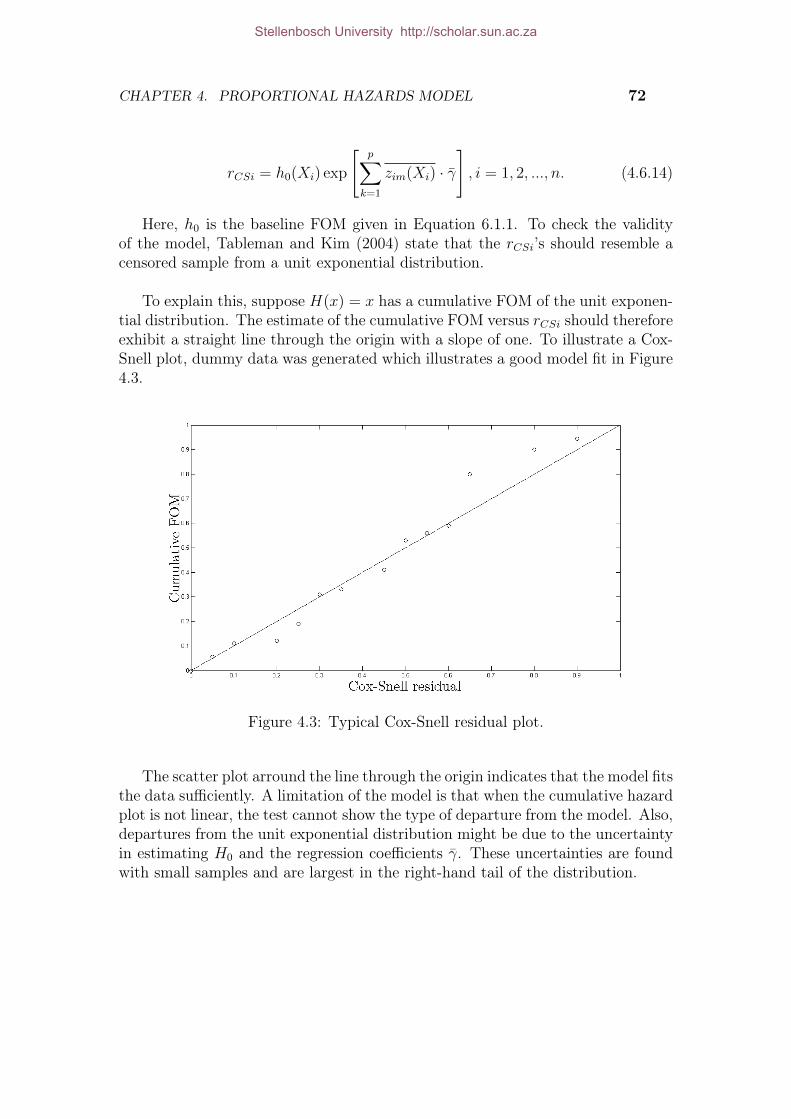
CHAPTER 4. PROPORTIONAL HAZARDS MODEL 72
rCSi = h0(Xi) exp
[p∑
k=1
zim(Xi) · γ], i = 1, 2, ..., n. (4.6.14)
Here, h0 is the baseline FOM given in Equation 6.1.1. To check the validityof the model, Tableman and Kim (2004) state that the rCSi’s should resemble acensored sample from a unit exponential distribution.
To explain this, suppose H(x) = x has a cumulative FOM of the unit exponen-tial distribution. The estimate of the cumulative FOM versus rCSi should thereforeexhibit a straight line through the origin with a slope of one. To illustrate a Cox-Snell plot, dummy data was generated which illustrates a good model fit in Figure4.3.
Figure 4.3: Typical Cox-Snell residual plot.
The scatter plot arround the line through the origin indicates that the model fitsthe data sufficiently. A limitation of the model is that when the cumulative hazardplot is not linear, the test cannot show the type of departure from the model. Also,departures from the unit exponential distribution might be due to the uncertaintyin estimating H0 and the regression coefficients γ. These uncertainties are foundwith small samples and are largest in the right-hand tail of the distribution.
Stellenbosch University http://scholar.sun.ac.za

CHAPTER 4. PROPORTIONAL HAZARDS MODEL 73
4.7 Decision ModelThis section deals with the development of a decision model based on ResidualUseful Life (RUL) and cost optimization. In the case of non-repairable systems,RUL and cost optimization estimations are based on the observed FOMs discussedin Section 4.4. These estimates are used to develop a decision model.
Several authors have developed decision such models based on cost optimizationand the relationship between RUL and the FOM (conditional probability of fail-ure), for example, Jardine (1973), Newby and Dagg, Pintelon and Gelders (1992),Wu and Ryan (2011), Lugtigheid et al. (2007), Makis and Jardine (1992),Newby(2008) and Banjevic et al. (2001).
Jardine (1973) presented decision models taking into account factors such asoperating cost, long term cost minimization, technological improvements, itemsprone to breakdown and minimization of downtime. Conventional renewal meth-ods attempt to minimize the long term operational cost of an item by finding anminimum cost level, known as the minimum long term Life Cycle Cost (LCC).
In order to determine the minimum long term LCC, two decision rules arediscussed in this section, namely (a) decision making with RUL estimation and(b) decision making aided by cost optimization.
4.7.1 Residual Life Estimation
Calculation of the RUL is based on the FOMs discussed in Section 4.4.1, i.e.Equation 6.1.1. Authors mentioned in the introduction of this section utilize theconditional event expectation of an item to determine RUL estimates. For thisreason this section deals with the conditional failure expectation.
This section makes use of three reliability functions, i.e. f(x), F (x) and R(x).To include the influence of covariates, the functions have to functions of time andcovariates, i.e. f(x, z(x)), F (x, z(x)) and R(x, z(x)). For generality, assume time-dependent covariates.
Suppose a decision policy for an item at time x states that the item should bereplaced at time Xp or at failure, whichever comes first. The conditional expecta-tion, Xr+1 ≤ Xp, can then be given by:
E[Xr+1 |Xr+1 ! Xp ] =
∫ Xp
xx · fX(x, z(x))dx∫ Xp
xfX(x, z(x))dx
(4.7.1)
Stellenbosch University http://scholar.sun.ac.za
CHAPTER 4. PROPORTIONAL HAZARDS MODEL 74
where the expected RUL to the (r + 1)th event can be given by:
µr+1 = E[Xr+1 |Xr+1 ! Xp ]− x (4.7.2)
A confidence interval can be estimated around the RUL in (4.7.1) to representthe certainty of the estimate. Let the upper confidence limit of the expectedresidual life be denoted by Xr+1, and the lower limit by X∼
r+1. Calculation of the
upper confidence level can be done by numerically solving:∫ X∼
r+1x
fX(x, z(x))dx
1−∫ x
0fX(x, z(x))dx−
∫∞Xp
fX(x, z(x))dx= 1− 1− CI
2(4.7.3)
where CI indicates the confidence interval. The lower limit is calculated simi-larly by numerically solving:
∫ X∼r+1
xfX(x, z(x))dx
1−∫ x
0fX(x, z(x))dx−
∫∞Xp
fX(x, z(x))dx= 1− CI
2(4.7.4)
However, in some cases it is required to determine the RUL when no preventivemaintenance rule is present, i.e. Xp = ∞. In this case the expected residual lifeat x ≈ 0 can be calculated using a modified version of Equation 4.7.1 given by:
E[Xr+1] =
∫∞0
x · fX(x, z(x))dx∫∞0
fX(x, z(x))dx(4.7.5)
and is known as the non-repairable system’s Mean Time Between Failure(MTBF). The expected RUL to the (r + 1)th event can be given by:
µr+1 = E[Xr+1]− x (4.7.6)
with the upper confidence interval equation given as:∫ Xr+1
0
fX(x, z(x))dx = 1− CI
2(4.7.7)
and the lower confidence interval equation given as:∫ X∼
r+1
0
fX(x, z(x))dx = 1−(1− CI
2
)(4.7.8)
To visualize RUL, a graphical illustration of the concepts is given in Figure 4.4.Suppose that the CM inspection interval for a specific non-repairable item is Xc.At each interval the RUL and corresponding confidence interval is indicated by a
Stellenbosch University http://scholar.sun.ac.za
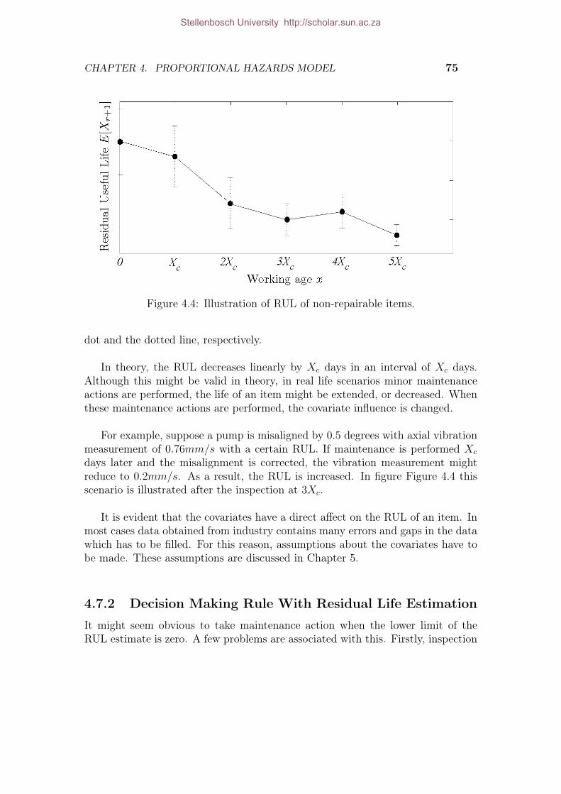
CHAPTER 4. PROPORTIONAL HAZARDS MODEL 75
Figure 4.4: Illustration of RUL of non-repairable items.
dot and the dotted line, respectively.
In theory, the RUL decreases linearly by Xc days in an interval of Xc days.Although this might be valid in theory, in real life scenarios minor maintenanceactions are performed, the life of an item might be extended, or decreased. Whenthese maintenance actions are performed, the covariate influence is changed.
For example, suppose a pump is misaligned by 0.5 degrees with axial vibrationmeasurement of 0.76mm/s with a certain RUL. If maintenance is performed Xc
days later and the misalignment is corrected, the vibration measurement mightreduce to 0.2mm/s. As a result, the RUL is increased. In figure Figure 4.4 thisscenario is illustrated after the inspection at 3Xc.
It is evident that the covariates have a direct affect on the RUL of an item. Inmost cases data obtained from industry contains many errors and gaps in the datawhich has to be filled. For this reason, assumptions about the covariates have tobe made. These assumptions are discussed in Chapter 5.
4.7.2 Decision Making Rule With Residual Life Estimation
It might seem obvious to take maintenance action when the lower limit of theRUL estimate is zero. A few problems are associated with this. Firstly, inspection
Stellenbosch University http://scholar.sun.ac.za

CHAPTER 4. PROPORTIONAL HAZARDS MODEL 76
intervals are performed discretely. However, if the lower limit was close to zero atthe inspections interval, it might decrease to zero between maintenance intervalsplacing the item at high risk of failure.
Secondly, RUL estimations are derived from the conditional failure expectationwhich has the consequence that it only reaches zero as time approaches infinity. Toovercome these problems, a decision rule is given as follows: maintenance action isbe taken as soon as the lower RUL limit minus the inspection period divided by twois less or equal to the time when the estimate is determined. This is representedas follows:
X∼r+1
−Xc/2 ≤ x (4.7.9)
where Xc the interval.
4.7.3 Cost Optimization Models
The objective of cost optimization models are to minimize the long term LCC ofan item. Two factors are balanced: (a) cost of preventive maintenance and (b) costof unexpected failure. Preventive maintenance is when maintenance is performedin attempt to prevent the occurrence of failure. Renewal maintenance is when anitem has already failed and need to be replaced. In Figure 4.5 these factors areplotted indicating the optimal instant when to perform maintenance.
Figure 4.5: Optimal maintenance instant.
Stellenbosch University http://scholar.sun.ac.za

CHAPTER 4. PROPORTIONAL HAZARDS MODEL 77
Let Cf indicate the cost of unexpected failure replacement and Cp the costof preventive replacement. Also, the time required for preventive replacement isrepresented by a, and the time required for failure replacement is represented byb. The total cycle cost of maintenance can be given by:
CXp = Cp ·RX(Xp, z(x)) + Cf · FX(Xp, z(x)) (4.7.10)
where RX and FX are defined in Chapter 2 as the reliability function andcumulative distribution function, respectively. It should be noted, even when anoptimum maintenance instant Xp is defined, expected failures might still occur.Furthermore, the expected duration of a non-repairable item’s life cycle at timex = 0 is given by:
E[Xp] = (Xp+a)·RX(Xp, z(x))+(E[Xr+1|Xr+1 ! Xp]+b)·FX(Xp, z(x)) (4.7.11)
Dividing Equation 4.7.10 by Equation 4.7.11 yields the cost of maintenance perunit time:
C(Xp) =Cp ·RX(Xp, z(x)) + Cf · FX(Xp, z(x))
(Xp + p) ·RX(Xp, z(x)) + (E[Xr+1 | Xr+1 ≤ Xp] + f) · F (Xp, z(x))(4.7.12)
where the minimum cost is found where dC(Xp)/dx = 0. Detailed inference ofthe model is given by Jardine (1973). Dummy-data was generated to plot C(Xp)in Figure 4.6 which indicates the minimum cost per unit time located near.
Figure 4.6: Long term cost per unit time optimization.
Stellenbosch University http://scholar.sun.ac.za

CHAPTER 4. PROPORTIONAL HAZARDS MODEL 78
4.7.4 Final Decision Model
At this moment, two estimations have been introduced, namely: (a) ResidualUseful Life and (b) long term cost optimization. It is not known which of the twoestimations would produce the best estimations for the event arrival time. Thesedecision models are presented here with an additional decision model.
• Decision model 1: Perform maintenance according to the residual useful lifeestimates, i.e.
X∼r+1
−Xc/2 ≤ x (4.7.13)
where X∼r+1
is the lower confidence limit, Xc the inspection interval and x
the current oil age in hours.
• Decision model 2: Perform maintenance according to the optimal point onthe cost function.
x = Xp (4.7.14)
where x is the current point in time and Xp the recommended preventivereplacement time.
• Decision model 3: Combine decision model 1 and 2 and perform maintenancewhenever either of the two decision models suggests that maintenance hasto be performed.
The decision models are applied to the case study in Chapter 5. The resultsare then compared and decided which model produces the best event arrival timepredictions.
4.8 ConclusionIn Chapter 4 two different forms of the PHM were presented, e.g. semi-parametricPHM and fully-parametric PHM. The fully-parametric Weibull PHM was foundto be the most suitable form identified for this thesis. An algorithm developed byCarstens et al. (2011) was found to be acceptable for parameter estimation of thefully-parametric Weibull PHM. Several Goodness-of-fit models were introducedwith which the model parameters could be tested. Lastly, two decision modelswere introduced whereby a third model was given which is a combinations of thesetwo decision models.
Stellenbosch University http://scholar.sun.ac.za

Chapter 5
Proportional Hazards ModelApplication
5.1 IntroductionThe Proportional Regression Model (PHM) investigated in Chapter 4 is appliedto data obtained in the South African mining industry which is then also used tovalidate the theory discussed in Chapter 4.
Most industries in South Africa do not know how reliability modelling can im-prove overall asset performance. As a result, there is a lack of commitment towardsthe recording of good quality data which cannot be used for reliability modelling.
Because data quality is such a problem, it was necessary to develop data re-quirements which can be used to evaluate data to determine whether it is suitablefor reliability modelling. After a long search of suitable data, data found at Sishensatisfied these requirements. Sishen is an open pit iron ore mine in the NorthernCape and is part of Anglo American (Kumba Iron Ore).
Sishen has several assets which have sophisticated Condition Monitoring (CM)equipment implemented on it. One of the crucial assets to Sishen’s operation istheir fleet of 78 haul trucks. As a result, it was decided to apply this thesis to dataobtained from these haul trucks to illustrate the benefit of reliability modelling.
Currently there are three truck manufacturer’s models in operation, namely:Caterpillar , Komatsu and Liebherr. The Caterpillar (CAT) trucks employ me-chanical drive powertrains. Komatsu and Liebherr on the other hand employdiesel-electric powetrains with a diesel generator which powers electric wheel-
79
Stellenbosch University http://scholar.sun.ac.za

CHAPTER 5. PROPORTIONAL HAZARDS MODEL APPLICATION 80
motors at each wheel.
It was found that the CAT trucks had the most readily available data andwas therefore chosen for this study. Sishen has eight CAT 793D trucks in op-eration. These are 78l diesel engines capable of producing 1742kW and moving218 ton payload. Each truck has an on-board Computerized Maintenance Man-agement System (CMMS) which monitors and records several conditions of thetruck. Also, Sishen has a state-of-the-art tribology center which analyzes oil sam-ples taken weekly from each truck.
This data was evaluated using the data requirements and is discussed Section5.2. Once it was established that the data was suitable, analysis and modellingthereof was done using the theory discussed in Chapter 3. This is discussed inSection 5.4. The decision model is then applied and discussed in Section 5.5.1.
5.2 Data RequirementsThe requirements given in this section was developed to evaluate data to determinewhether it is suitable to be used for Proportional Hazards Modelling modelling.For the sake of the discussion, it is assumed that the process parameter is time,such as hours. Other process parameters are discussed in Chapter 2.
5.2.1 Events
Firstly, it is necessary to define an event. Events might include any of the following:
• Preventative and scheduled maintenance: Typically, this is minor mainte-nance actions such as lubrication and realignment which affects the influencethat the covariates has on the FOM.
• Failure replacement: When an item or system is replaced.
• Censored items: This might be an item which has been taken out of operationor not have not yet failed at the time when the observation period ended.
Events are when maintenance action is taken which influenced the item survivaltime. Given this information, it is important to know the time when any of theseevents occurred. It is also necessary to know when the item was put into operation.Lastly, to develop a meaningful PHM, a minimum of approximately 15 events arerequired. In order for covariates to converge, sufficient events are necessary withwhich the PHM is constructed.
Stellenbosch University http://scholar.sun.ac.za
CHAPTER 5. PROPORTIONAL HAZARDS MODEL APPLICATION 81
5.2.2 Covariates
Covariates are explanatory variables that may be predictive of the outcome understudy. Two types of covariates were introduced in Chapter 2, namely: (a) quanta-tive-covariates and (b) subjective-covariates.
Quantative covariates Condition Monitoring (CM) recordings which include(but are not limited to): temperature, vibration, pressure, oil content and stress.Quantitative covariates may be time-dependent or time-independent and can ei-ther be measured continuously or measured at a fixed intervals. These covariatesshould be recorded at each possible instant and a recoding is necessary at eachevent occurrence.
Subjective may covariates are binary variables representing factors such as:whether oil changed at each service interval, type of oil used, maintenance teamused, type of installation set up, supplier used and operator on shift. Dependingon the data, this is basically comprises of yes/no data.
One method to obtain subjective data can be to speak with the technical per-sonnel that maintain and run the items. With their knowledge and experience it iseasier find the correct subjective covariates which contributes to the occurrence ofevents. Another method to obtain subjective data through CMMS systems withwhich the data can be recorded.
5.2.3 Requirements
In conclusion, the main requirements of data to perform Proportional HazardsModelling is:
• Time: The time when the item was put into operation and the time whenevents occurred.
• Covariates: Recordings of all possible covariate values should be done at thetime of each event. It is also preferred that covariate values are recordedbetween events. Covariate recordings made between event occurrences, maybe done continuously and/or discretely, depending on the CM equipmentinstalled and maintenance strategy followed.
These requirements are necessary to develop a PHM. Later in this chapter itis shown how assumptions about data can bare made to adhere to these require-ments. It should therefore be noted that if given data does not exactly fit these
Stellenbosch University http://scholar.sun.ac.za

CHAPTER 5. PROPORTIONAL HAZARDS MODEL APPLICATION 82
requirements it does not necessarily mean that it cannot be used. For this reasonthese data requirements should merely be used as guidelines for data to develop aPHM.
5.3 CAT 793D DataData was obtained from the CAT 793D haul trucks operating at Sishen. Figure5.1 illustrates an CAT 793D haul truck fully loaded. Two types of diagnostic ofdata recorded namely: a.) on-board Condition Monitoring measurements and b.)results of oil analysis sample data.
Figure 5.1: Cat 793D haul truck.
For the purpose of this thesis, all the conditions related to the diesel enginecondition was used for PHM development. Therefore, from this point forward datarelated to the condition of the related to the engine of the haul trucks are takeninto account and all other data is ignored.
Stellenbosch University http://scholar.sun.ac.za
CHAPTER 5. PROPORTIONAL HAZARDS MODEL APPLICATION 83
5.3.1 On-Board Measurements
Each truck has an Electronic Control Module (ECM) which utilizes engine manage-ment software to monitor, protect and control the engine utilizing its’ diagnosticsensors to measure several important conditions of the truck. These sensors takeinto account operating conditions and power requirements to adapt the engine suchthat maximum performance and efficiency are achieved. On board measurementsused are:
• Air filter pressure (max.) [kPa].
• Ambient air temperature (avg.) [◦C].
• Boost pressure (avg.) [kPa].
• Engine coolant temperature (avg.) [◦C].
• Oil filter pressure (max.) [kPa].
• Oil filter pressure (min.) [kPa].
• Left exhaust temperature (max.) [◦C].
• Right exhaust temperature (max.) [◦C].
• Right after cooler temperature (max.) [◦C].
On-board measurements are made hourly whereby the maximum or averagefor that hour is taken. The ECM has “alarm” triggers which sound when a certaincondition reaches an unacceptable level. Additional to the alarm signal in thecockpit, a signal is sent to a remote computer at the maintenance center. Thesealarms can be bypassed to shut them off, ignoring the alarm. Switching off thesealarms might be attributed to one of two reasons.
Firstly, the driver is busy loading the truck and cannot stop the shift to takethe truck to maintenance. Secondly, the driver switches the alarm off because theydo not believe it would lead to failure.
If the alarms are ignored it places the haul truck at risk of engine failure. Ifthe engine fails, the haul truck is taken out of service for a period of time fargreater than that of the time required for preventive replacement. Due to thedependency upon the haul trucks for operation, taking a haul truck out of servicefor an extended period of time has major financial implications. For this reason,
Stellenbosch University http://scholar.sun.ac.za

CHAPTER 5. PROPORTIONAL HAZARDS MODEL APPLICATION 84
the necessary measuremens should be taken to avoid the occurrence of failure.
With this being said, a haul truck consists of several thousand components.For this reason the ECM cannot precisely indicate which component is faultythereby placing several components at risk of failure if an alarm is ignored. Thisfurther motivates the need to develop a model which can be used to estimate whenfailure is likely to occur. This in turn would reduce the maintenance engineers’uncertainty about the failure behaviour of the haul trucks.
5.3.2 Oil Analysis
Oil samples are taken weekly whereby analysis thereof provides the constituentsin the oil in parts per million (ppm). Some of the constituents found in the oil are:
• Iron [Fe]
• Chrome [Cr]
• Lead [Pb]
• Copper [Cu]
• Silica [Sn]
• Aluminium [Al]
• Nickel [Ni]
• Gold [Ag]
• Silicone [Si]
• Barium [Ba]
• Nitrous [Na]
• Magnesium [Mg]
• Calcium [Ca]
• Zinc [Zn]
Different forms of viscosity are also determined when oil analysis is done. Theseinclude:
• Viscosity I [VI]
• Viscosity 40 [V40]
• Viscosity 100 [V100]
According to the engineers at the tribolgy center, some of the most influentialelements found in the oil are: Fe, Si and V100. These elements can be used todetermine, to some extent, how the engine is deteriorating. For example, degrada-tion of components such as cylinders, gears, pistons, shafts and valves is indicatedby the Fe found in oil.
Stellenbosch University http://scholar.sun.ac.za

CHAPTER 5. PROPORTIONAL HAZARDS MODEL APPLICATION 85
Furthermore, due to the dusty environment the haul trucks operate in, dustis sucked up through the air filters. The dust contains a large amount of Si andhigh levels present in the oil might indicate that the air filters or gasket seals aredegrading and need replacement.
Lastly, V100 is an indication of the viscosity of the oil and can indicate fueldilution, mixture of oils and water in oil. Fuel dilution is indicated by low V100levels which means traces of diesel are found in the oil. When diesel is found inthe oil a fuel component might be faulty and replacement thereof has to be donebefore failure occurs and other components are damaged.
These are three of the most important oil analysis measurements found to in-dicate degradation of the haul truck engines. Each measured value is compared tothree predefined values, namely: maximum value, minimum value and maximumgradient. Values outside the predefined maximum and minimum values initializemaintenance inspection and/or oil change. If the gradient level is reached, thetrend in the element value surpasses the predefined value indicating that a compo-nent is degrading faster than it should and maintenance teams need to determinethe cause.
Oil samples not only contain the constituent values, it also contain the oil sam-ple date and the age of the oil in hours. A major problem the tribology centeris experiencing is that maintenance technicians are topping up the oil of the haultruck’s when it is being fuelled. Adding new oil to old oil dilutes the old oil whichhas the consequence that oil analysis results are inaccurate. It wouldn’t be a prob-lem if the precise amount of oil and time of the oil addition was recorded but nosuch attempt is being made.
As a rule, the oil of a truck is changed after 750 hours. Therefore the mainte-nance tactic followed is a combination of Condition Based Maintenance and UsageBased Maintenance discussed in Chapter 2.
5.3.3 Maintenance Decisions
At Sishen, maintenance is mainly based on oil analysis results. On-board record-ings are rarely used to determine maintenance instances. Maintenance is initializedif one of the three constituent limits are reached. Although these procedures mightbe set in place, it is a conservative method in that the constituents are taken intoaccount individually. The problem with this is that failure might be brought uponby more than one constituent. For this reason, a prognostic model such as the
Stellenbosch University http://scholar.sun.ac.za

CHAPTER 5. PROPORTIONAL HAZARDS MODEL APPLICATION 86
PHM is used to determine the correlation between several constituents and failure.
For this reason it is possible to include on-board recorded values in conjunctionwith oil analysis values to develop a PHM model which describes the underlyingfailure behaviour of the haul trucks.
5.4 Weibull PHM FitIn order to determine the most appropriate model fit is an iterative process. Inorder to develop the best model fit, Goodness-of-Fit (GOF) test and technicalexperience gained during this project were used. The main objective of modeldevelopment is to determine the most appropriate covariates for a good model fit.
The process of model development is given below.
• Data manipulation.
• Covariate selection.
• Goodness-of-fit tests.
• Final Model.
A detail discussion of these items are presented in the following sections wherebyit is shown how the final Weibull PHM was developed.
5.4.1 Data Manipulation
In this section all the assumptions made about the data are discussed. The periodfor which data was obtained for each of the eight trucks was approximately fromOctober 2010 to June 2011.
Once the on-board truck data and oil analysis were obtained, the next step wasto combine the data. However, because on-board measurements are made hourlyand oil samples taken weekly, it was necessary to “fill the gaps” between the oilsample data points to have oil data for each on-board measurement.
When the data was combined two problems were identified. Firstly, data be-tween weekly oil samples had to be interpolated. To overcome this problem, theengineers at the tribolgy center suggested that between weekly oil samples shouldbe interpolated linearly.
Stellenbosch University http://scholar.sun.ac.za

CHAPTER 5. PROPORTIONAL HAZARDS MODEL APPLICATION 87
Figure 5.2: Extrapolation of oil data.
For example, suppose that oil samples were taken in week 3 and week 4 indi-cating Fe values of = 21 ppm and = 24.2 ppm. The data is then interpolated fromweek 3 to week 4 as shown in Figure 5.2. This meant that there was correspondingoil sample data for each on-board data measurement.
The second problem found was that oil changes had taken place between oilsamples and it was not indicated when it took place. To solve this problem con-sider Figure 5.3. Suppose that the oil data is known at weeks 7, 8, 9 and 10. Theoil age at these weeks are: 326, 446, 98 and 198.
Due to the fact that the oil age in week 10 is less than the oil hours in week8, an oil change occurred between week 8 and 10. Data was then extrapolatedlinearly from week 10 backwards to the point where Fe is zero. This point wastherefore where an oil change had taken place. Then, the Fe (ppm) was kept con-stant from week 8 to where the oil change took place. It was kept constant dueto the uncertainty of which might have happened right before the oil change tookplace. Although this assumption might be conservative, the decision was basedupon the knowledge of the engineers of the tribology center.
In order to validate the final model, 7 of the 8 trucks were used to develop thefinal Weibull PHM model. The model was then applied to the 8th truck’s data tovalidate its ability to model the failure behaviour of this haul truck.
Stellenbosch University http://scholar.sun.ac.za

CHAPTER 5. PROPORTIONAL HAZARDS MODEL APPLICATION 88
Figure 5.3: Extrapolation of oil data.
The haul trucks have similar failure patterns and deciding which haul truck touse for validation was trivial. It was decided to choose haul truck number 4 duethe fact that the period over which data was available for this haul tuck containedsufficient observations to validate the model. Further discussions about the modelvalidation is done in Section 5.5.
As for the other 7 haul trucks, 19 events were observed for the given period oftime. Table 1 is a tabulation of these 19 events with the corresponding haul truck,failure time (Xi) and failure type (Ci).
In Table 1 it can be seen that 19 events were observed of which 4 were failuresand 15 were censored observations. An event table which contains the 15 covari-ates at each event can be seen in Table A.1. Due to the vast amount of data usedin this study it is not possible to include all of it in this thesis.
Table 5.2 is an extract of 4 of the 16th event’s measured covariates. Table A.2 isan extract of all of the 1st event’s measured covariates. Deciding which covariatesto use for the model played an important part in this project and is discussed next.
5.4.2 Covariate Selection
Selecting covariates for this study was initially done based on the experience ofthe engineers at the tribolgy center and technicians at the maintenance workshop.
Stellenbosch University http://scholar.sun.ac.za

CHAPTER 5. PROPORTIONAL HAZARDS MODEL APPLICATION 89
Table 5.1: Event table.
Haul truck Xi Ci
1 1 552.00 02 2 418.32 03 2 561.00 04 3 634.67 05 3 538.00 07 4 530.00 08 4 384.00 09 4 444.00 010 4 341.00 06 4 445.00 011 5 486.42 012 5 385.00 013 5 872.00 014 6 454.00 015 6 399.00 016 6 904.00 117 7 562.00 018 7 222.18 119 7 422.64 020 7 338.00 021 8 840.00 022 8 48.40 123 8 105.60 124 8 324.00 0
The engineers are of the opinion that the most influential oil data covariates are:Fe, Si, Na, V100, Pb and Cu.
A combined total of 15 covariates were therefore used. All of these covariateswere believed to contribute to failure in some way. To determine the most appro-priate covariates for a good Weibull PHM fit, different covariate combinations haveto be analyzed. In order to determine the quality of an model fit, Goodness-of-Fit(GOF) tests are used.
Stellenbosch University http://scholar.sun.ac.za

CHAPTER 5. PROPORTIONAL HAZARDS MODEL APPLICATION 90
Table 5.2: An extract of the 16th event’s measured covariates.
# x Ci
Rig
htA
fter
cool
erte
mpe
ratu
re[◦
C]
Eng
ine
oilp
ress
ure
[kPa]
Fe[p
pm]
Si[p
pm]
16 811.05 0 60.00 455.50 0.1934 3.780716 812.05 0 60.00 454.00 0.1936 3.789416 813.05 0 60.00 459.50 0.1939 3.798216 814.05 0 60.00 454.00 0.1942 3.807016 815.05 0 55.00 468.5 0.1944 3.8157
5.4.3 Goodness-of-fit Tests
Three GOF tests were discussed in Chapter 3, namely: Kolmogorov-Smirnoff,Anderson-Darling and Cos-Snell. Compared to the other two tests, the Kolmogorov-Smirnoff (K-S) test is more flexible and less complex to use. For these reasons theK-S test was the chosen GOF test for model fit evaluation.
The process of the K-S test was presented in Chapter 3 and is briefly repeatedhere for convenience. The basic principle of the K-S test is defined by the followingtwo hypothesis:
• H0: The data follows a specified distribution Fn(x) = F0(x).
• H1: The data does not follow the specified distribution Fn(x) &= F0(x).
The K-S test attempts to find the maximum vertical distance between thecumulative Probability Density Function (PDF) and the Empirical DistributionFunction (EDF). This vertical distance is known as the test statistic, Dn, and is
Stellenbosch University http://scholar.sun.ac.za

CHAPTER 5. PROPORTIONAL HAZARDS MODEL APPLICATION 91
given by:Dn = max|F (xi)− F0(xi)| (5.4.1)
The test statistic is compared to a critical value, cnjα, using the test conditiongiven by:
Dn > cnjα (5.4.2)
where cnjα is obtained from the K-S One-Sample statistic table. If Dn exceedsthe cnjα there is not sufficient evidence to reject the null-hypothesis. With 19events n = 19 and a confidence interval of 95% α = 0.05 and cnjα = 0.301. Severaldifferent covariate combinations were evaluated. However, only the 3 most impor-tant combinations of interest is discussed in detail.
For each combination, the model fitting procedure discussed in Chapter 3 wasapplied to determine the model parameters, i.e. β, η and γ. In each case thecumulative PDF is determined using these estimations. The EDF is determinedusing Equation 3.6.1 in Chapter 3.
Several covariate combinations were analyzed to determine the best combina-tion to develop a Weibull PHM model which best describes the underlying failurebehaviour of the item under study. The combinations which produced the bestmodel fit is presented with its’ corresponding model parameters and solution toEquation 3.4.9 in Chapter 3 maximized for parameter estimation.
5.4.3.1 Covariate Combination 1
The first combination consisted of Fe, boost pressure, left exhaust temperatureand engine oil filter pressure. The calculated test statistic, Dn, is equal to 0.2129.According to Equation 5.4.2, the K-S test statistic for this combination is lessthan the critical value indicating that there is enough evidence to reject the nullhypothesis. In return, this indicates that the model developed the this covariatecombination is acceptable. A plot of the cumulative PDF and the EDF are givenin Figure 5.4.
The test statistic, model parameters and log-likelihood value obtained withthis covariate combination is given in Table 5.3.
Although this combinations provides an acceptable model fit, further investiga-tion has to be done to determine whether another covariate combination providesbetter a model fit.
Stellenbosch University http://scholar.sun.ac.za

CHAPTER 5. PROPORTIONAL HAZARDS MODEL APPLICATION 92
Figure 5.4: Covariate combination: Fe, boost pressure, left exhaust temperatureand engine filter oil pressure (min).
Table 5.3: Covariate combination: Fe, boost pressure, left exhaust temperatureand engine oil pressure.
Dn 0.2129β 0.9617η 6260.6033γ1 −1.2043γ2 0.0197γ3 −0.0049γ4 −4.6237
log-likelihood 6899.9
5.4.3.2 Covariate Combination 2
For the third combination the Fe, right after cooler temperature and engine coolanttemperature covariates were used. For this particular scenario, Dn, is equal to0.2105 indicating that there is enough evidence to reject the null hypothesis whichmeans that this model is acceptable. A plot of the cumulative PDF and the EDFis given in Figure 5.5.
The test statistic, model parameters and log-likelihood value obtained with
Stellenbosch University http://scholar.sun.ac.za
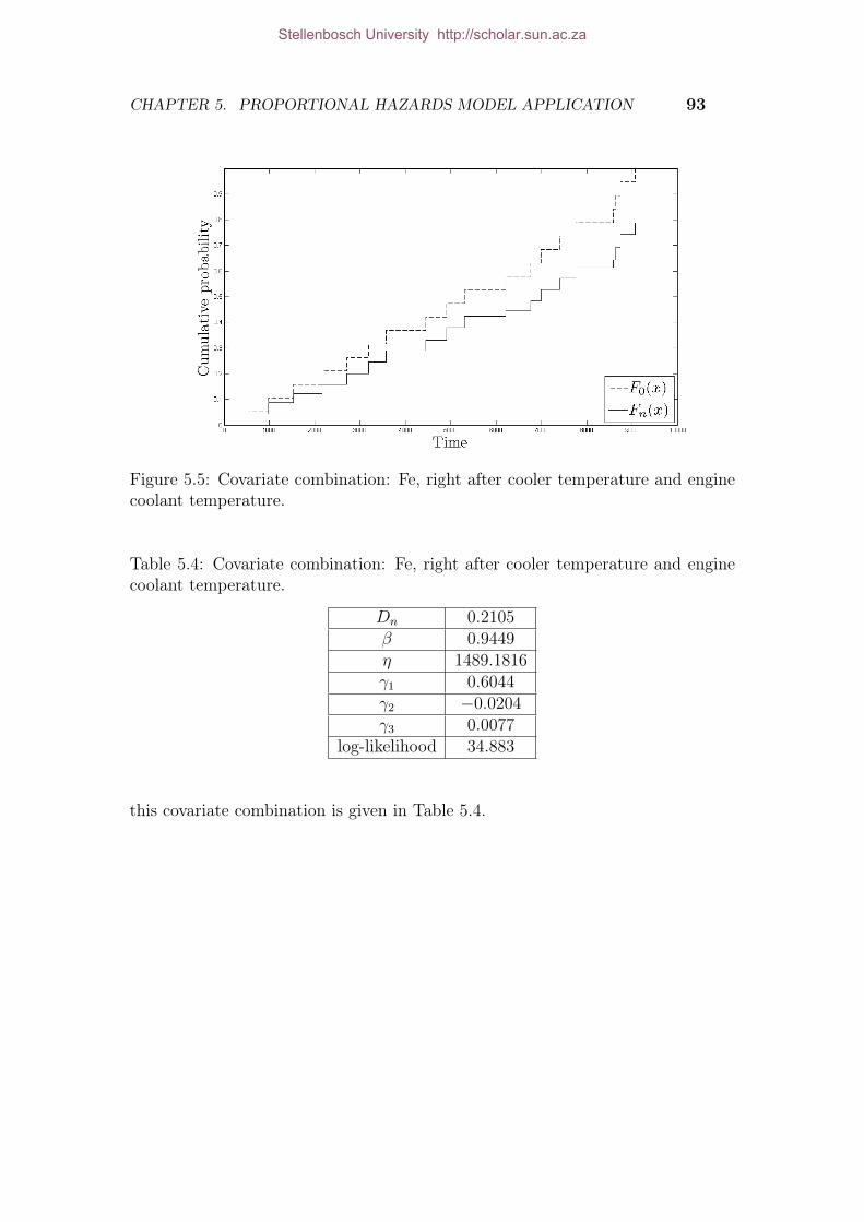
CHAPTER 5. PROPORTIONAL HAZARDS MODEL APPLICATION 93
Figure 5.5: Covariate combination: Fe, right after cooler temperature and enginecoolant temperature.
Table 5.4: Covariate combination: Fe, right after cooler temperature and enginecoolant temperature.
Dn 0.2105β 0.9449η 1489.1816γ1 0.6044γ2 −0.0204γ3 0.0077
log-likelihood 34.883
this covariate combination is given in Table 5.4.
Stellenbosch University http://scholar.sun.ac.za

CHAPTER 5. PROPORTIONAL HAZARDS MODEL APPLICATION 94
Table 5.5: Covariate combination: Fe, boost pressure and left exhaust temp.
Dn 0.1731β 0.883η 365.542γ1 0.394γ2 0.026γ3 −0.011
log-likelihood 34.8226
5.4.3.3 Covariate Combination 3
The final combination consisted of Fe, boost pressure and left exhaust tempera-ture. The calculated test statistic, Dn, is equal to 01731 which meant that there isenough evidence to reject the null hypothesis indicating that the covariates usedprovide an acceptable model fit. A plot of the cumulative PDF and the EDF isgiven in Figure 5.6.
Figure 5.6: Covariate combination: Fe, boost pressure and left exhaust temp.
The test statistic, model parameters and log-likelihood value obtained withthis covariate combination is given in Table 5.5.
Stellenbosch University http://scholar.sun.ac.za
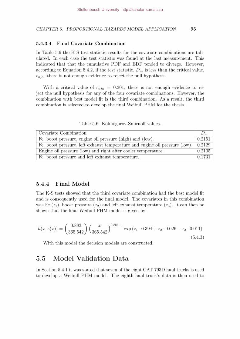
CHAPTER 5. PROPORTIONAL HAZARDS MODEL APPLICATION 95
5.4.3.4 Final Covariate Combination
In Table 5.6 the K-S test statistic results for the covariate combinations are tab-ulated. In each case the test statistic was found at the last measurement. Thisindicated that that the cumulative PDF and EDF tended to diverge. However,according to Equation 5.4.2, if the test statistic, Dn, is less than the critical value,cnjα, there is not enough evidence to reject the null hypothesis.
With a critical value of cnjα = 0.301, there is not enough evidence to re-ject the null hypothesis for any of the four covariate combinations. However, thecombination with best model fit is the third combination. As a result, the thirdcombination is selected to develop the final Weibull PHM for the thesis.
Table 5.6: Kolmogorov-Smirnoff values.
Covariate Combination Dn
Fe, boost pressure, engine oil pressure (high) and (low). 0.2151Fe, boost pressure, left exhaust temperature and engine oil pressure (low). 0.2129Engine oil pressure (low) and right after cooler temperature. 0.2105Fe, boost pressure and left exhaust temperature. 0.1731
5.4.4 Final Model
The K-S tests showed that the third covariate combination had the best model fitand is consequently used for the final model. The covariates in this combinationwas Fe (z1), boost pressure (z2) and left exhaust temperature (z3). It can then beshown that the final Weibull PHM model is given by:
h(x, z(x)) =
(0.883
365.542
)( x
365.542
)0.883−1
exp (z1 · 0.394 + z2 · 0.026− z3 · 0.011)
(5.4.3)With this model the decision models are constructed.
5.5 Model Validation DataIn Section 5.4.1 it was stated that seven of the eight CAT 793D haul trucks is usedto develop a Weibull PHM model. The eighth haul truck’s data is then used to
Stellenbosch University http://scholar.sun.ac.za

CHAPTER 5. PROPORTIONAL HAZARDS MODEL APPLICATION 96
Table 5.7: Validation truck event’s table.
# Ci Xi Z1(X1) [ppm] Z2(X2) [kPa] Z3(X3) [◦C]1 0 530 0.24 172.5 6782 0 384 0.16 151 6313 0 445 0.11 179.5 6724 1 341 0.2259 185 6515 0 445 0.24 182.5 662
validate the model. From this point forward this haul truck is referred to as thevalidation truck. This section discusses how the data of the validation truck wasmodified to be able to use it in the decision model.
The same data manipulation procedures, as discussed in Section 5.4.1, are ap-plied to the validation truck. Five events were observed in the validation truckdata, four of which was censored observations and one failure. These events aretabulated in Table 5.7.
Where Z1(X1), Z2(X2) and Z3(X3) represent Fe, boost pressure and left ex-haust temperature. In order to test the validity of the model it has to be appliedto the validation truck data and predict the time of the events. The validationtruck data is handled as follows:
(i.) Data up to a specified inspection point Xc is extracted from an event’shistory. This decision is based on the fact that oil samples are taken weekly,i.e. every 168 hours. For this reason it is assumed that it is most practicalto specify data up to this point.
(ii.) A prediction of the data is then made into the future from the point ofinspection, up to the point where the survivor function approaches.
Due to the fact that there is no data available onwards from the point of in-spection, future covariate behaviour has to be extrapolated into the unknown.Procedures considered for future covariate behaviour prediction was keeping thecovariate value constant and fitting a trend line to the data up to the time of theinspection.
Several attempts were undertaken where the covariate values were taken tobe constant into the future. A problem with this method was that the reliabilityfunctions were totally erroneous due to the fact that RUL estimations were in most
Stellenbosch University http://scholar.sun.ac.za
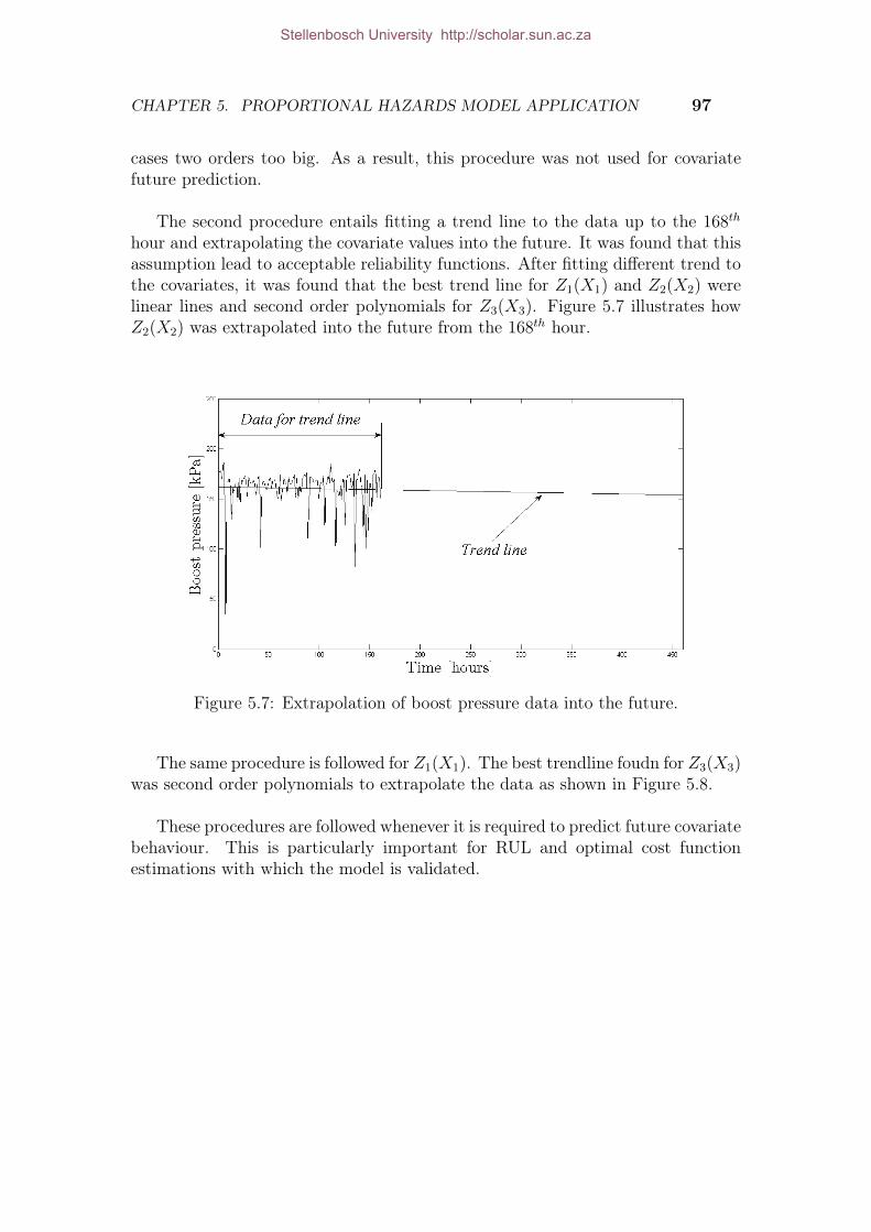
CHAPTER 5. PROPORTIONAL HAZARDS MODEL APPLICATION 97
cases two orders too big. As a result, this procedure was not used for covariatefuture prediction.
The second procedure entails fitting a trend line to the data up to the 168thhour and extrapolating the covariate values into the future. It was found that thisassumption lead to acceptable reliability functions. After fitting different trend tothe covariates, it was found that the best trend line for Z1(X1) and Z2(X2) werelinear lines and second order polynomials for Z3(X3). Figure 5.7 illustrates howZ2(X2) was extrapolated into the future from the 168th hour.
Figure 5.7: Extrapolation of boost pressure data into the future.
The same procedure is followed for Z1(X1). The best trendline foudn for Z3(X3)was second order polynomials to extrapolate the data as shown in Figure 5.8.
These procedures are followed whenever it is required to predict future covariatebehaviour. This is particularly important for RUL and optimal cost functionestimations with which the model is validated.
Stellenbosch University http://scholar.sun.ac.za

CHAPTER 5. PROPORTIONAL HAZARDS MODEL APPLICATION 98
Figure 5.8: Extrapolation of left exhaust temperature data into the future.
5.5.1 Decision Model
In Chapter 3, three decision model approaches were introduced, namely: (a) Resid-ual Useful Life and (b) long term cost optimization. The decision models arerepeated here for convenience sake.
• Decision model 1: Perform maintenance according to the residual useful lifeestimates, i.e.
X∼r+1
−Xc/2 ≤ x (5.5.1)
where X∼r+1
is the lower confidence limit, Xc the inspection interval and x
the current oil age in hours.
• Decision model 2: Perform maintenance according to the optimal point onthe cost function.
x = Xp (5.5.2)
where x is the current point in time and Xp the recommended preventivereplacement time.
• Decision model 3: Combine decision model 1 and 2 and perform maintenancewhenever either of the two decision models suggests that maintenance hasto be performed.
Stellenbosch University http://scholar.sun.ac.za

CHAPTER 5. PROPORTIONAL HAZARDS MODEL APPLICATION 99
After each model is presented, the models are compared to establish whichmodel produces the best event arrival time predictions. It is assumed that deci-sion model predictions can be made when weekly oil samples are taken. For thisreason, the decision models determine event arrival predictions on a weekly basis.
Due to the fact that oil samples are taken weekly, i.e. every 168 hours, predic-tions are made every 168 hours. Additional to the weekly predictions, predictionsare also made at the time of the event itself.
5.5.2 Decision model 1: Residual Useful Life Estimates
The decision model for RUL estimates state that maintenance is done wheneverthe lower RUL confidence limit reduces to less than the inspection interval dura-tion Xc, i.e. 168 hours. Note, predictions and estimates are used interchangeablyin this chapter.
5.5.2.1 Event 1
The first event occurred in the 530th hour. Figure 5.9 illustrates the three RULestimates at hours 168, 338 and 530, respectively. At each estimate the confidencelimits are illustrated by vertical lines. At the 168th hour, the RUL estimate isE[Xr+1]=369 hours with upper and lower confidence limits of Xr+1 = 419 andX∼
r+1= 303 hours, respectively.
According to Equation 5.5.1, X∼r+1
−Xc/2 = 215 and x = 168 which means that
maintenance should not be performed due to the fact that 215 " 168. Please note,from this point forward the results are directly compared and not given separately.
At the 338th hour, the RUL estimate is E[Xr+1]=1561 hours with confidencelimits of Xr+1 = 2018 and X∼
r+1−Xc/2 = 753 hours, respectively. The increased
prediction might be an indication that the condition of the haul truck improvedsince the previous prediction was made. As a result, maintenance should not beperformed due to the fact that 665 " 338. The first two estimates indicated thatmaintenance should not have been performed which, according to the actual eventtime, is correct.
The final prediction made at the 530th hour produced a RUL estimate ofE[Xr+1]=543 hours with confidence limits of 618 and X∼
r+1− Xc/2 = 542 hours,
respectively. Due to the fact that 454 ≤ 530, it is suggested that maintenance
Stellenbosch University http://scholar.sun.ac.za

CHAPTER 5. PROPORTIONAL HAZARDS MODEL APPLICATION 100
Figure 5.9: Validation truck event 1.
should be performed which coincides with the actual event arrival time and there-fore an accurate prediction.
5.5.2.2 Event 2
The second event occurred in the 384th hour. Figure 5.10 illustrates the threeRUL estimates at hours 168, 338 and 384, respectively. At the 168th hour, theRUL estimate is E[Xr+1]=180 hours with confidence limits of Xr+1 = 207 andX∼
r+1= 170 hours, respectively.
According to Equation 5.5.1, X∼r+1
−Xc/2 = −86 and x = 168 which indicates
that maintenance has to be performed because 82 ≤ 168.
The prediction at the 338th hour indicated that the RUL estimation is E[Xr+1]=623hours with confidence limits of Xr+1 = 648 and X∼
r+1= 605 hours, respectively.
Maintenance should not be performed due to the fact that 517 " 338. At the 384th
hour, the RUL estimate is E[Xr+1]=820 hours with confidence limits of Xr+1 = 849and X∼
r+1= 779 hours, respectively. Maintenance should not be performed due to
the fact that 691 " 384.
Stellenbosch University http://scholar.sun.ac.za

CHAPTER 5. PROPORTIONAL HAZARDS MODEL APPLICATION 101
Figure 5.10: Validation truck event 2.
The first prediction proved to be conservative which meant that maintenancewould have been done far too early. The last two estimations were found to beless conservative than the first prediction. However, maintenance decisions basedon the estimates for the second event would not have been satisfactorily.
5.5.2.3 Event 3
The third event occurred in the 444th hour. Figure 5.11 illustrates the three RULestimates at hours 168, 338 and 444, respectively. At the 168th hour, the RUL esti-mate is determined to be E[Xr+1]=502 hours with confidence limits of Xr+1 = 580and X∼
r+1= 384 hours, respectively.
According to Equation 5.5.1, X∼r+1
− Xc/2 = 296 and x = 168 which meant
that the decision model does not suggest that maintenance should be taken, i.e.296 " 168.
The second prediction at the 338th hour is E[Xr+1]=879 hours with confidencelimits of Xr+1 = 1039 and X∼
r+1= 604 hours, respectively. Maintenance should
not be performed at this point due to the fact that 516 " 444. At the 444th hour,the RUL estimate is E[Xr+1]=626 hours with confidence limits of Xr+1 = 680 andX∼
r+1= 537 hours, respectively. Maintenance should also not be performed due to
Stellenbosch University http://scholar.sun.ac.za

CHAPTER 5. PROPORTIONAL HAZARDS MODEL APPLICATION 102
Figure 5.11: Validation truck event 3.
the fact that 449 " 444.
However, at the time of the event at the 444th hour, the prediction that main-tenance action should be taken at the 449th hour is a good result even though itdoes not exactly represent reality. Estimates for the third event proved that themodel had accurately predicted the the haul truck’s third event and performingmaintenance based on the decision model predictions would have been successful.
5.5.2.4 Event 4
The fourth event took place in the 341th hour. Figure 5.11 illustrates three RULestimates at hours 168, 337 and 341, respectively. The first prediction at the 168thhour indicated that the RUK estimate E[Xr+1]=519 hours with confidence limitsof Xr+1 = 636 and X∼
r+1= 353 hours, respectively.
According to Equation 5.5.1, maintenance should not be performed at thispoint due to the fact that X∼
r+1−Xc/2 = 265 and x = 168 and 265 " 168.
The RUL prediction at the the 338th hour is E[Xr+1]=447 hours with confidencelimits of Xr+1 = 473 and X∼
r+1= 412 hours, respectively. In this case maintenance
should be performed due to the fact that 324 ≤ 338. The final prediction at the341st hour indicated that the RUL is E[Xr+1]=567 hours with confidence limits
Stellenbosch University http://scholar.sun.ac.za
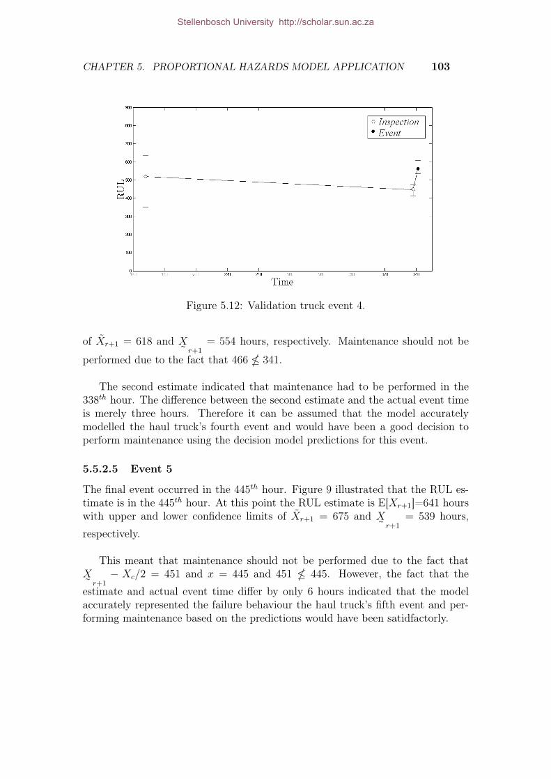
CHAPTER 5. PROPORTIONAL HAZARDS MODEL APPLICATION 103
Figure 5.12: Validation truck event 4.
of Xr+1 = 618 and X∼r+1
= 554 hours, respectively. Maintenance should not be
performed due to the fact that 466 " 341.
The second estimate indicated that maintenance had to be performed in the338th hour. The difference between the second estimate and the actual event timeis merely three hours. Therefore it can be assumed that the model accuratelymodelled the haul truck’s fourth event and would have been a good decision toperform maintenance using the decision model predictions for this event.
5.5.2.5 Event 5
The final event occurred in the 445th hour. Figure 9 illustrated that the RUL es-timate is in the 445th hour. At this point the RUL estimate is E[Xr+1]=641 hourswith upper and lower confidence limits of Xr+1 = 675 and X∼
r+1= 539 hours,
respectively.
This meant that maintenance should not be performed due to the fact thatX∼
r+1− Xc/2 = 451 and x = 445 and 451 " 445. However, the fact that the
estimate and actual event time differ by only 6 hours indicated that the modelaccurately represented the failure behaviour the haul truck’s fifth event and per-forming maintenance based on the predictions would have been satidfactorly.
Stellenbosch University http://scholar.sun.ac.za

CHAPTER 5. PROPORTIONAL HAZARDS MODEL APPLICATION 104
Figure 5.13: Validation truck event 5.
5.5.2.6 Conclusion
Estimations made for events one and four indicated that maintenance had to beperformed. This would have been good decisions due to the fact that it was accu-rate predictions of the actual event arrival times. However, estimations made forevents three and five indicated that maintenance had to be performed a few hoursafter the actual event arrival time. Due to the fact that these predictions wereinaccurate by a few hours, it was assumed that it would have resulted in goodmaintenance decisions.
The overall accuracy of the estimates would have ensured that good decisionswould have been made if the model was used to determine maintenance instantswhich in essence is the development of ACPs.
5.5.3 Decision model 2: Long Term Cost Optimization
The costs considered in this section are approximate maintenance costs. Due tocompany policies it is not possible to obtain exact maintenance costs. Costs wereestimated to be Cp = R65 000 for preventive maintenance and Cf = R1 600 000for failure maintenance. As with the RUL estimates, a cost function estimate wasdetermined at each inspection interval and time of event. Cost function estimatesfound in this section were found using Equation 3.7.12 in Chapter 3.
Stellenbosch University http://scholar.sun.ac.za
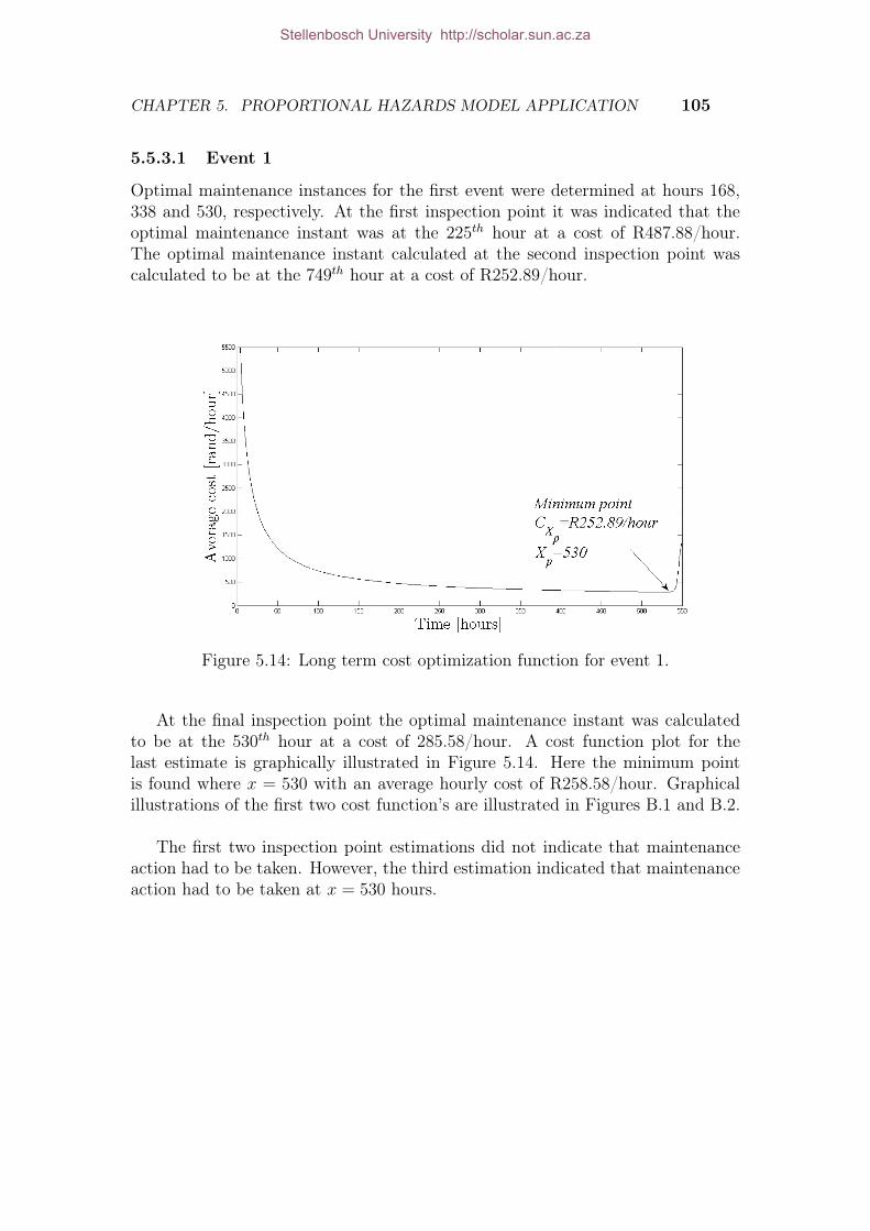
CHAPTER 5. PROPORTIONAL HAZARDS MODEL APPLICATION 105
5.5.3.1 Event 1
Optimal maintenance instances for the first event were determined at hours 168,338 and 530, respectively. At the first inspection point it was indicated that theoptimal maintenance instant was at the 225th hour at a cost of R487.88/hour.The optimal maintenance instant calculated at the second inspection point wascalculated to be at the 749th hour at a cost of R252.89/hour.
Figure 5.14: Long term cost optimization function for event 1.
At the final inspection point the optimal maintenance instant was calculatedto be at the 530th hour at a cost of 285.58/hour. A cost function plot for thelast estimate is graphically illustrated in Figure 5.14. Here the minimum pointis found where x = 530 with an average hourly cost of R258.58/hour. Graphicalillustrations of the first two cost function’s are illustrated in Figures B.1 and B.2.
The first two inspection point estimations did not indicate that maintenanceaction had to be taken. However, the third estimation indicated that maintenanceaction had to be taken at x = 530 hours.
Stellenbosch University http://scholar.sun.ac.za
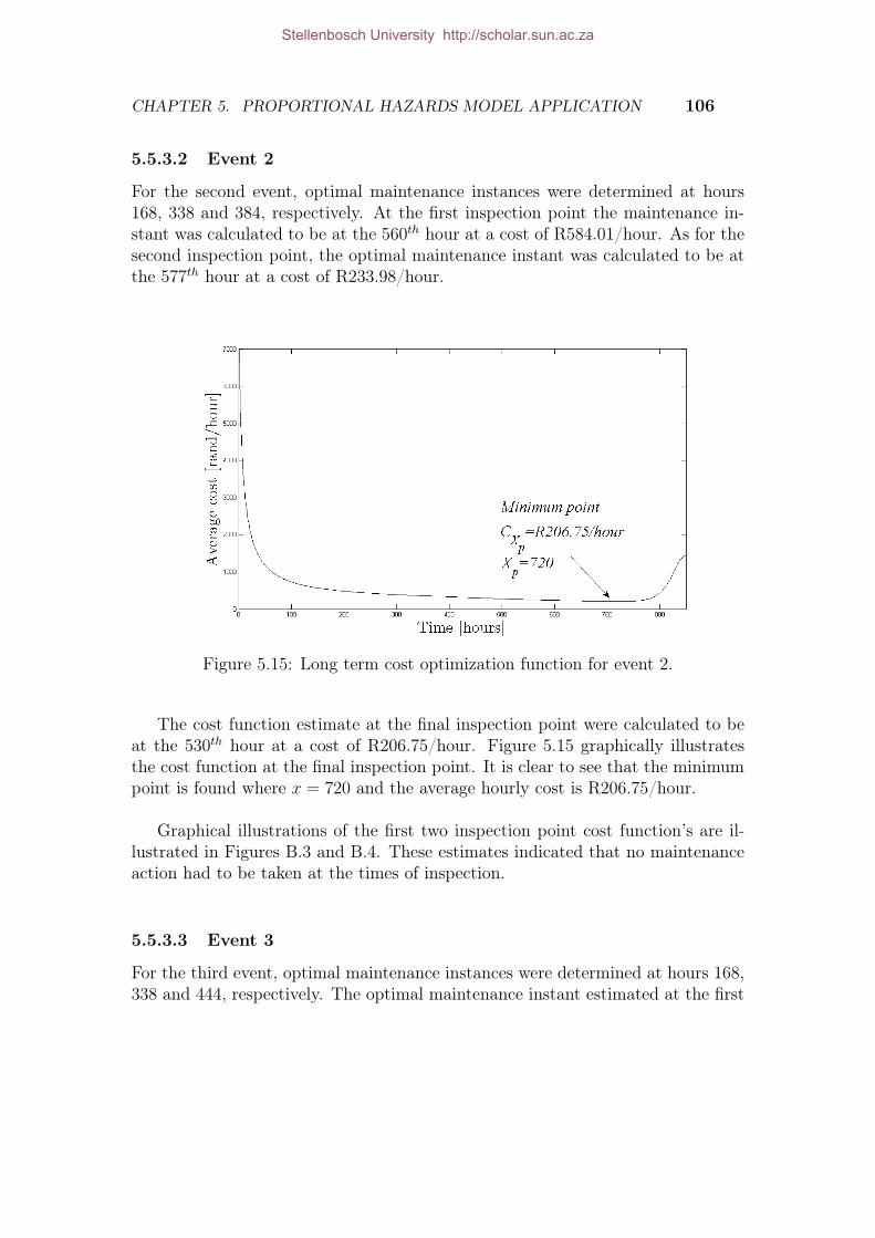
CHAPTER 5. PROPORTIONAL HAZARDS MODEL APPLICATION 106
5.5.3.2 Event 2
For the second event, optimal maintenance instances were determined at hours168, 338 and 384, respectively. At the first inspection point the maintenance in-stant was calculated to be at the 560th hour at a cost of R584.01/hour. As for thesecond inspection point, the optimal maintenance instant was calculated to be atthe 577th hour at a cost of R233.98/hour.
Figure 5.15: Long term cost optimization function for event 2.
The cost function estimate at the final inspection point were calculated to beat the 530th hour at a cost of R206.75/hour. Figure 5.15 graphically illustratesthe cost function at the final inspection point. It is clear to see that the minimumpoint is found where x = 720 and the average hourly cost is R206.75/hour.
Graphical illustrations of the first two inspection point cost function’s are il-lustrated in Figures B.3 and B.4. These estimates indicated that no maintenanceaction had to be taken at the times of inspection.
5.5.3.3 Event 3
For the third event, optimal maintenance instances were determined at hours 168,338 and 444, respectively. The optimal maintenance instant estimated at the first
Stellenbosch University http://scholar.sun.ac.za

CHAPTER 5. PROPORTIONAL HAZARDS MODEL APPLICATION 107
inspection point was calculated to be at the 293th hour at a cost of R443.06/hour.At the second inspection point, the optimal maintenance instant was determinedto be at the 506th hour at a cost of R316.8/hour.
Figure 5.16: Long term cost optimization function for event 3.
The final inspection point indicated that the optimal maintenance inspectioninstance was found to be at the 459th hour at a cost of R317/hour. A cost functionplot for the estimate is graphically illustrated in Figure 5.16 where the minimumpoint is found at x = 577 where the average hourly cost is R317/hour. Graphi-cal illustrations of the first two cost functions are illustrated in Figures B.5 and B.6.
These estimates indicated that no maintenance action had to be taken at thetimes of inspection.
5.5.3.4 Event 4
Optimal maintenance instances was calculated at hours 168, 338 and 341, respec-tively. At the first inspection point, the optimal maintenance instant was calcu-lated to be at the 272th hour at a cost of R418.39/hour. The optimal maintenaceinstant calculatd at the second inspection point was found to be at the 374th hourat a average cost of R419.37/hour.
Stellenbosch University http://scholar.sun.ac.za

CHAPTER 5. PROPORTIONAL HAZARDS MODEL APPLICATION 108
Figure 5.17: Long term cost optimization function for event 4.
Calculation of the optimal maintenance instance at the final inspection pointwas determined to be at the 526th hour at a cost of R293.93/hour. The final inspec-tion point cost function graphically illustrated in Figure 5.17 where the minimumpoint is found at x = 577 where the average hourly cost is R293.93/hour. Graph-ical illustrations of the first two inspection point cost functions are illustrated inFigures B.7 and B.8.
These estimates indicated that no maintenance action had to be taken at thetimes of inspection.
5.5.3.5 Event 5
Only one optimal maintenance instant calculation was done for the fifth event. Itwas found that the optimal instant was calculated to be at the 472nd hour at acost of R359.10/hour. The cost function is graphically illustrated in Figure 5.18where the minimum point is found at x = 472 at an average cost of R359.10/hour.This estimate did not suggest that maintenance action had to be taken.
5.5.3.6 Conclusion
Although most of the results given in this section indicated that maintenance hadto be performed later than the actual event arrival times, the overall accuracy of
Stellenbosch University http://scholar.sun.ac.za

CHAPTER 5. PROPORTIONAL HAZARDS MODEL APPLICATION 109
Figure 5.18: Long term cost optimization function for event 5.
the model to represent the failure behaviour of the haul trucks were satisfactory.If this decision model is used it would not prevent al the failures but it is a goodrepresentation of reality.
For this reason, the estimates determined in this section would also have en-sured fairly accurate maintenance decisions would have been made if this mainte-nance decision model was used with the developed Weibull PHM.
5.5.4 Decision model 3: Combining decision model 1 anddecision model 2.
This section combines results obtained with decision model 1 and decision model 2in order to develop the third decision model. Results obtained at each inspectionpoint for each respective event for both the first and second decision models aretabulated in Table 5.5.4. The third decision model adopts the earliest predictionof the other two decision models. For example, in Table 5.5.4 the first and sec-ond event arrival times of the first and second decision models are 215 and 225,respectively. In this case the third decision model would adopt the first decisionmodel’s result because 215≤225.
The next step is to determine which model is best suited for maintenancescheduling. For each inspection result a percentage error value is determined.
Stellenbosch University http://scholar.sun.ac.za

CHAPTER 5. PROPORTIONAL HAZARDS MODEL APPLICATION 110
Percentage error values are calculated using the following expression:
%error = abs(event time − model decision time
event time) (5.5.3)
Calculating the percentage error values determines which decision model pre-dicted the time of event most accurately. The percentage error illustrates the errorof the decision model prediction based on the actual arrival time of the event. Thismethod compares the decision models in a crude but effective way. The total foreach error percentage column can be seen in Table 5.5.4.
The minimum total percentage error value indicates the best decision modelfor maintenance scheduling due to the fact that it exhibits the least deviation frompredicting the correct event arrival times. Therefore the decision best suited formaintenance intervention scheduling is the second decision model.
Table 5.8: Criteria 1 and 2 combination.
Decision Model1 2 3
Xr+1 −Xc/2 MA % Error Xp MA % Error MA % Error215 No 0.59434 225 No 0.575472 No 0.59434327 Yes 0.383019 749 No 0.413208 No 0.383019454 Yes 0.143396 530 Yes 0 Yes 0.14339682 Yes 0.786458 560 No 0.458333 No 0.786458517 No 0.346354 577 No 0.502604 No 0.346354691 No 0.799479 720 No 0.875 No 0.799479296 No 0.333333 293 No 0.34009 No 0.34009324 Yes 0.27027 506 No 0.13964 No 0.27027466 No 0.04955 459 No 0.033784 No 0.033784265 No 0.222874 272 No 0.202346 No 0.222874324 Yes 0.27027 374 No 0.157658 No 0.27027466 No 0.04955 526 No 0.184685 No 0.04955451 No 0.013483 472 No 0.060674 No 0.013483
Total: 4.262 Total: 3.943 Total: 4.253
Stellenbosch University http://scholar.sun.ac.za
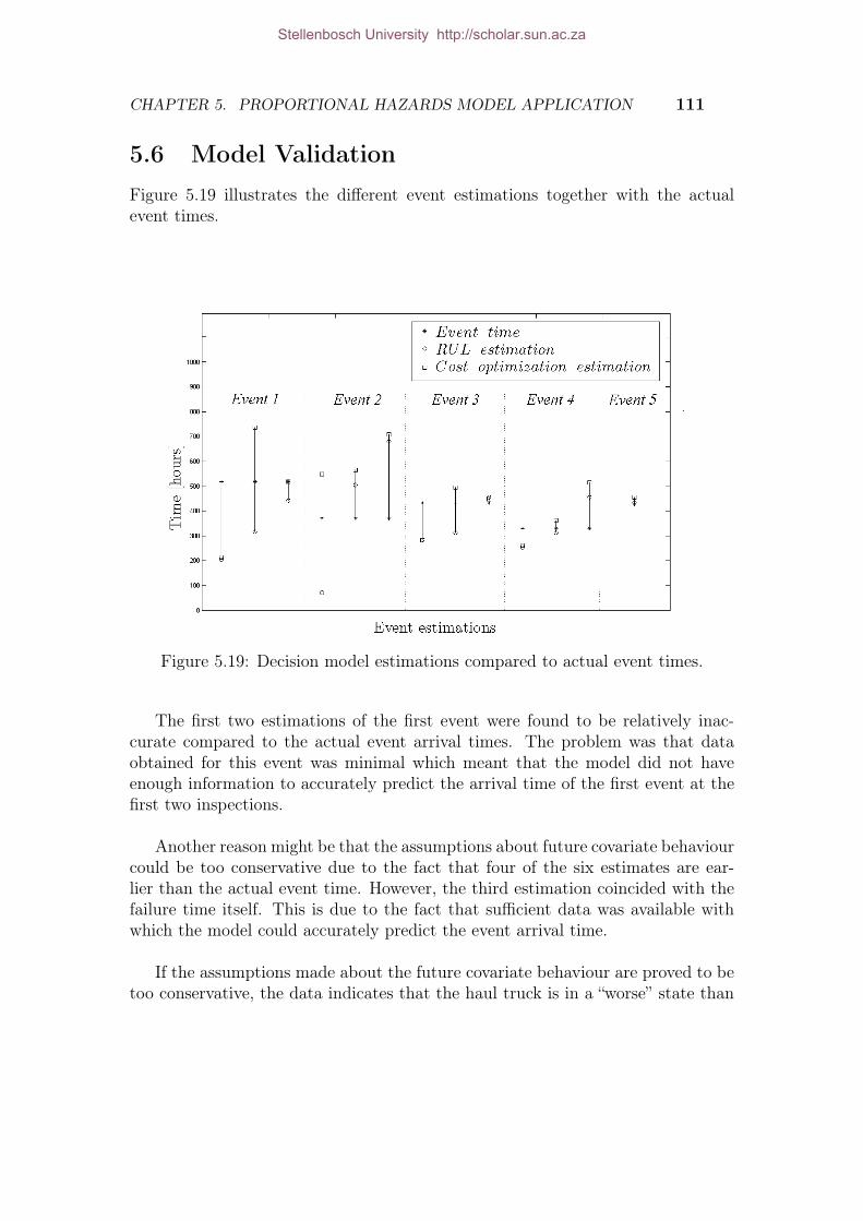
CHAPTER 5. PROPORTIONAL HAZARDS MODEL APPLICATION 111
5.6 Model ValidationFigure 5.19 illustrates the different event estimations together with the actualevent times.
Figure 5.19: Decision model estimations compared to actual event times.
The first two estimations of the first event were found to be relatively inac-curate compared to the actual event arrival times. The problem was that dataobtained for this event was minimal which meant that the model did not haveenough information to accurately predict the arrival time of the first event at thefirst two inspections.
Another reason might be that the assumptions about future covariate behaviourcould be too conservative due to the fact that four of the six estimates are ear-lier than the actual event time. However, the third estimation coincided with thefailure time itself. This is due to the fact that sufficient data was available withwhich the model could accurately predict the event arrival time.
If the assumptions made about the future covariate behaviour are proved to betoo conservative, the data indicates that the haul truck is in a “worse” state than
Stellenbosch University http://scholar.sun.ac.za

CHAPTER 5. PROPORTIONAL HAZARDS MODEL APPLICATION 112
it actually is which results in conservative estimations. If however the assumptionsmade about the future covariate behaviour are proven to exhibit a high level ofrisk, the data indicates that the truck is in a “healthier” state than it actually iswhich lead to estimations with a certain level of risk.
Estimations of the second event were also found to be slightly inaccurate. Fur-ther investigation indicated that several assumptions had to be made about thecovariates. Seeing that five of the six estimations (RUL and cost optimization)were later than the actual failure times, assumptions regarding future covariatebehaviour were exposed to allowing too high a level of risk.
Relative to the actual event times, the final three event estimates proved to besufficiently acceptable. Estimates of the third event were rather conservative dueto the fact that three of the estimates were earlier than the actual event times.As a consequence, assumptions regarding future covariate behaviour for this eventproved too conservative. Final estimates of the fourth event indicated that theassumptions regarding future covariate behaviour were exposed to allowing toohigh a level of risk.
5.7 ConclusionThis chapter looked at the third item of the research methodology. It presentedthe development of the final Weibull PHM development and its application to aCAT 793D haul truck engine data. Results indicated that the accuracy of pre-dicting future event arrival times proved to be accurate compared to the actualevent arrival times. As a result, the final Weibull PHM is a good representationof the actual failure behaviour of the CAT 793D haul truck used for the case study.
The final Weibull PHM developed in this thesis, satisfactorily predicted eventarrival times of a CAT 793D haul truck. Decision models were evaluated and itwas concluded that the long term cost optimization decision model proved to bemost successful and can be considered for ACP development.
Stellenbosch University http://scholar.sun.ac.za

Chapter 6
Conclusion and Recommendations
6.1 OverviewChapter 1 indicated that a large amount of wasted maintenance activities are beingperformed. For this reason, industry is experiencing an increased interest in Phys-ical Asset Management (PAM) to improve maintenance activities. The conceptof PAM comprises of several Key Performance Areas (KPAs) such as Asset CarePlans (ACPs). These ACPs consist of many tactical maintenance strategies. Us-age based Maintenance (UBM) bases its maintenance activities on historical failuredata, not taking into account the condition of the item. Condition Based Main-tenance (CBM) bases its maintenance activities on Condition Monitoring (CM)information, disregarding the historical failure data.
Each of these strategies take into account one type of data disregarding otherdata. For this reason, the problem undertaken in this thesis was to research modelswhich take into account both types of data. Therefore, the objective of this studywas to research the relevant literature in order to gain a detailed understanding ofthe models which can be used to incorporate both types of data.
Chapter 2 presented a comprehensive literature study which lead to Prognos-tics as a solution to the problem. It was then indicated that it might be possibleto use regression models and it was therefore found necessary to investigate re-gression models.
Chapter 3 evaluated six regression models according to four criteria which re-flected the applicability of each model to achieve the objectives of the thesis. Theseevaluations were compared revealing that the PHM is the most suitable model forthis thesis.
113
Stellenbosch University http://scholar.sun.ac.za

CHAPTER 6. CONCLUSION AND RECOMMENDATIONS 114
In Chapter 4, two different forms of the PHM were discussed indicating thatthe fully-parametric Weibull PHM was found to be the most suitable form of thePHM. Parameter estimation of the fully-parametric form was done using an algo-rithm developed by Carstens et al. (2011). Several Goodness-of-fit models wereintroduced with which the model parameters could be tested. Lastly, three deci-sion models were proposed with the third model being a combinations of the firstand second decision model.
Chapter 5 presented the development of the final Weibull PHM and its appli-cation to a CAT 793D haul truck engine data. The Weibull PHM model is givenby:
h(x, z(x)) =
(β
η
)(x
η
)β−1
exp(zi(x) · γ
)(6.1.1)
Suitable data for the study was found at the open pit iron ore mine in theNorthern Cape, Sishen. Validation of the Weibull PHM was done using the fol-lowing procedure:
1. Fit the Weibull PHM to seven of the eight haul trucks’ data.
2. Apply the developed model to the data obtained from the eighth truck todetermine how accurate the estimates represent its failure behaviour.
Estimations obtained with the model indicated that the model was a relativelygood representation of reality compared to the actual event arrival times. Thethree decision models were evaluated and it was concluded that the long term costoptimization decision model proved to be most successful and can be consideredfor ACP development assistance.
Two major benefits of the developed model are: a) The possibility of makingrelatively accurate estimations compared to the arrival times of events; and b)Reduced dependence on the expertise and experience of engineers and techniciansfor maintaining assets. In conclusion, from the obtained results it is concludedthat the Weibull PHM is a good representation of reality.
Although the Weibull PHM provided satisfactorily results, there is still roomfor improvement. In Section 6.2 three recommendations are given with which theaccuracy of the obtained result can be improved.
Stellenbosch University http://scholar.sun.ac.za

CHAPTER 6. CONCLUSION AND RECOMMENDATIONS 115
Findings from this study provide an exciting basis for the development of futureWeibull PHMs that could result in huge maintenance cost savings and reducedfailure occurrences.
6.2 Recommendations for Future ResearchExperience gained through completing this thesis has led to three recommendationsfor future research:
i ) Future covariate behaviour: The decision models applied in this thesis re-quired that assumptions regarding future covariate behaviour had to be made.In Section 5.5 it was stated that the use of future covariate behaviour pre-dictions elevate the importance of a more intricate understanding into thebehaviour of these covariates. Consequently, it is vital that future research in-clude comprehensive technique studies for predicting future covariate behaviourmore accurately.
ii ) Observed event composition: The majority of events in the data used werecensored observations. The implication is that the developed model is essen-tially modelling current maintenance behaviour to determine preventive main-tenance action. Due to the fact that the results obtained in this study accu-rately represented these observations means that the PHM has great potentialfor future research.
It is recommended that for future research, obtained data should contain agreater number of observed failures than censored observations. This recom-mendation only introduces the concept that better data could improve on thealready satisfactorily result obtained in this research project.
iii ) Data quality: The quality of data found in the South African industry re-mains a problem. As PAM gains popularity, greater commitment towards goodquality data recordings will be practised. Despite the fact that the data usedfor this study was lacking quality, acceptable and interpretable results wereobtained. It is therefore recommended that this thesis can be used to illustrateto industry the potential of failure data analysis.
These recommendations can be used to improve results obtained with futureresearch projects.
Stellenbosch University http://scholar.sun.ac.za

List of References
Andersen, P. (1982). Testing goodness of fit of cox’s regression and life model. Biometrics,pp. 67–77.
Anderson, T. and Darling, D. (1954). A test of goodness of fit. Journal of the AmericanStatistical Association, pp. 765–769.
Ascher, H. and Feingold, H. (1984a). Repairable systems reliability: modeling, inference,misconceptions and their causes. M. Dekker. ISBN 0824772768.
Ascher, H.E. and Feingold, H. (1984b). Repairable systems reliability: Modeling, infer-ence, misconceptions and their causes. Marcel Dekker.
Balakrishnan, n. and Rao, C. (2004). Handbook of Statistics 23. Elsevier, North Holland.
Banjevic, D. and Jardine, A. (2006). Calculation of reliability function and remaininguseful life for a markov failure time process. IMA Journal of Management Mathematics,vol. 17, no. 2, p. 115.
Banjevic, D., Jardine, A., Makis, V. and Ennis, M. (2001). A control-limit policy andsoftware for condition-based maintenance optimization. INFOR-OTTAWA-, vol. 39,no. 1, pp. 32–50.
Barnard, G. (1963). Some logical aspects of the fiducial argument. Journal of the RoyalStatistical Society. Series B (Methodological), pp. 111–114.
Bekker, J. (2011). Simulation notes. Stellenbosch University Industrial Department.
Bennett, S. (1983a). Analysis of survival data by the proportional odds model. Statisticsin Medicine, vol. 2, no. 2, pp. 273–277.
Bennett, S. (1983b). Log-logistic regression models for survival data. Applied Statistics,pp. 165–171.
Bonabeau, E., Dorigo, M. and Theraulaz, G. (1999). Swarm intelligence: from naturalto artificial systems. 1. Oxford University Press, USA.
Breslow, N. (1975). Analysis of survival data under the proportional hazards model.International Statistical Review/Revue Internationale de Statistique, pp. 45–57.
116
Stellenbosch University http://scholar.sun.ac.za
LIST OF REFERENCES 117
Caesarendra, W., Niu, G. and Yang, B. (2010). Machine condition prognosis based onsequential monte carlo method. Expert Systems with Applications, vol. 37, no. 3, pp.2412–2420.
Carstens, W., Vlok, P. and Visser, T. (2011). Estimation of multivariate proportionalhazards model parameters with artificial bee colony optimization. ORION.
Cheng, S., Wei, L. and Ying, Z. (1995). Analysis of transformation models with censoreddata. Biometrika, vol. 82, no. 4, p. 835.
Cheung, Y.B., Yip, P.S.F. and Karlberg, J.P.E. (2001). Fetal growth, early postnatalgrowth and motor development in pakistani infants. International Journal of Epidemi-ology, , no. 30, pp. 66–74.
Chinnam, R. and Baruah, P. (2003). Autonomous diagnostics and prognostics throughcompetitive learning driven HMM-based clustering. In: Neural Networks, 2003. Pro-ceedings of the International Joint Conference on, vol. 4, pp. 2466–2471. IEEE. ISBN0780378989. ISSN 1098-7576.
Chinnam, R. and Baruah, P. (2004). A neuro-fuzzy approach for estimating mean residuallife in condition-based maintenance systems. International Journal of Materials andProduct Technology, vol. 20, no. 1, pp. 166–179.
Ciampi, A. and Etezadi-Amoli, J. (1985). A general model for testing the proportionalhazards and the accelerated failure time hypotheses in the analysis of censored survivaldata with covariates. Communications in Statistics-Theory and Methods, vol. 14, no. 3,pp. 651–667.
Coetzee, J. (1997). The role of NHPP models in the practical analysis of maintenancefailure data. Reliability Engineering & System Safety, vol. 56, no. 2, pp. 161–168. ISSN0951-8320.
Cox, D. (1972a). Regression models and life tables. Journal of the Royal StatisticalSociety Series, vol. 1, p. 187 220. ISSN 21.
Cox, D. (1972b). Regression models and life-tables. Journal of the Royal StatisticalSociety. Series B (Methodological), pp. 187–220.
Cox, D. (1975). Partial likelihood. Biometrika, vol. 62, no. 2, pp. 269–276.
Cox, D. and Snell, E. (1968). A general definition of residuals. Journal of the RoyalStatistical Society. Series B (Methodological), pp. 248–275.
Dale, C. (1985). Application of the proportional hazards model in the reliability field.Reliability Engineering, vol. 10, no. 1, pp. 1–14. ISSN 0143-8174.
Stellenbosch University http://scholar.sun.ac.za
LIST OF REFERENCES 118
Deloux, E., Castanier, B. and Bérenguer, C. (2009). Predictive maintenance policy fora gradually deteriorating system subject to stress. Reliability Engineering & SystemSafety, vol. 94, no. 2, pp. 418–431. ISSN 0951-8320.
Elsayed, E., Liao, H. and Wang, X. (2006). An extended linear hazard regression modelwith application to time-dependent dielectric breakdown of thermal oxides. IIE Trans-actions, vol. 38, no. 4, pp. 329–340.
Endrenyi, J., Aboresheid, S., Allan, R., Anders, G., Asgarpoor, S., Billinton, R., Chowd-hury, N., Dialynas, E., Fipper, M., Fletcher, R. et al. (2001). The present status ofmaintenance strategies and the impact of maintenance on reliability. Power Systems,IEEE Transactions on, vol. 16, no. 4, pp. 638–646. ISSN 0885-8950.
Etezadi-Amoli, J. and Ciampi, A. (1987). Extended hazard regression for censored sur-vival data with covariates: a spline approximation for the baseline hazard function.Biometrics, pp. 181–192.
Feng, D., Xuefeng, H. and Jiyong, C. (2009). Reliability assessment based on equipmentcondition vibration feature using proportional hazards model. Journal of MechanicalEngineering, p. 12.
Fogel, G. (). Pas55 delegate material. Asset Management Course at Stellenbosch Uni-versity in Conjunction with Pragma.
Ghasemi, A., Yacout, S. and Ouali, M. (2009). Parameter estimation for condition basedmaintenance with proportional hazard model.
Goldman, J. (1967). Stochastic point processes: limit theorems. The Annals of Mathe-matical Statistics, vol. 38, no. 3, pp. 771–779.
Goode, K., Moore, J. and Roylance, B. (2000). Plant machinery working life predictionmethod utilizing reliability and condition-monitoring data. Proceedings of the Insti-tution of Mechanical Engineers, Part E: Journal of Process Mechanical Engineering,vol. 214, no. 2, pp. 109–122.
Gorjian, N., Ma, L., Mittinty, M., Yarlagadda, P. and Sun, Y. (2010). A review onreliability models with covariates.
Heiman, G. (2010). Basic statistics for the behavioral sciences. Wadsworth Pub Co.
Heng, A. (2000). Intelligent Prognostics of Machinery Health Using Suspended ConditionMonitoring Data.
Heng, A., Zhang, S., Tan, A. and Mathew, J. (2009). Rotating machinery prognos-tics: State of the art, challenges and opportunities. Mechanical Systems and SignalProcessing, vol. 23, no. 3, pp. 724–739. ISSN 0888-3270.
Stellenbosch University http://scholar.sun.ac.za

LIST OF REFERENCES 119
Isermann, R. (2005). Model-based fault-detection and diagnosis-status and applications.Annual Reviews in control, vol. 29, no. 1, pp. 71–85. ISSN 1367-5788.
Jardine, A. (1973). Maintenance, Replacement and Reliability. The Copp Clark Publish-ing Company.
Jardine, A., Anderson, P. and Mann, D. (1987). Application of the weibull propor-tional hazards model to aircraft and marine engine failure data. Quality and reliabilityengineering international, vol. 3, no. 2, pp. 77–82.
Jardine, A., Banjevic, D., Wiseman, M., Buck, S. and Joseph, T. (2001). Optimizinga mine haul truck wheel motors condition monitoring program use of proportionalhazards modeling. Journal of Quality in Maintenance Engineering, vol. 7, no. 4, pp.286–302.
Jardine, A., Lin, D. and Banjevic, D. (2006). A review on machinery diagnostics andprognostics implementing condition-based maintenance. Mechanical systems and signalprocessing, vol. 20, no. 7, pp. 1483–1510. ISSN 0888-3270.
Jiang, S., Landers, T. and Reed Rhoads, T. (2006). Proportional intensity models ro-bustness with overhaul intervals. Quality and Reliability Engineering International,vol. 22, no. 3, pp. 251–263.
Kacprzynski, G., Sarlashkar, A., Roemer, M., Hess, A. and Hardman, B. (2004). Pre-dicting remaining life by fusing the physics of failure modeling with diagnostics. JOMJournal of the Minerals, Metals and Materials Society, vol. 56, no. 3, pp. 29–35.
Kalbfleisch, J.D. and Prentice, R.L. (1980). The Statistical Analysis of Fialure TimeData. John Wiley and Sons, New York.
Karaboga, D. (2005). An idea based on honey bee swarm for numerical optimization.Techn. Rep. TR06, Erciyes Univ. Press, Erciyes.
Karaboga, D. and Akay, B. (2009). A comparative study of artificial bee colony algorithm.Applied Mathematics and Computation, vol. 214, no. 1, pp. 108–132.
Kelly, A. and Eastburn, K. (1982). Terotechnology. a modern approach to plant engineer-ing. Physical Science, Measurement and Instrumentation, Management and Education-Reviews, IEE Proceedings A, vol. 129, no. 2, pp. 131–136.
Kim, Y., Rizzoni, G. and Utkin, V. (2001). Developing a fault tolerant power-traincontrol system by integrating design of control and diagnostics. International Journalof Robust and Nonlinear Control, vol. 11, no. 11, pp. 1095–1114. ISSN 1099-1239.
Kirmani, S. and Gupta, R. (2001). On the proportional odds model in survival analysis.Annals of the Institute of Statistical Mathematics, vol. 53, no. 2, pp. 203–216. ISSN0020-3157.
Stellenbosch University http://scholar.sun.ac.za

LIST OF REFERENCES 120
Klein, J. and Moeschberger, M. (2003). Survival analysis: techniques for censored andtruncated data. Springer Verlag.
Krishnaiah, P.R. and Sen, P.K. (1984). Handbook of Statistics, Nonparametric Methods,vol. 4. North Holland, Amsterdam.
Kvaloy, J. and Lindqvist, B. (1998). Ttt-based tests for trend in repairable systems data.Reliability Engineering & System Safety, vol. 60, no. 1, pp. 13–28.
Kwan, C., Zhang, X., Xu, R. and Haynes, L. (2003). A novel approach to fault diagnosticsand prognostics. In: Robotics and Automation, 2003. Proceedings. ICRA’03. IEEEInternational Conference on, vol. 1, pp. 604–609. IEEE. ISBN 0780377362. ISSN1050-4729.
Li, Y., Kurfess, T. and Liang, S. (2000). Stochastic prognostics for rolling elementbearings. Mechanical Systems and Signal Processing, vol. 14, no. 5, pp. 747–762.
Lin, D., Oakes, D. and Ying, Z. (1998). Additive hazards regression with current statusdata. Biometrika, vol. 85, no. 2, p. 289.
Louit, D., Pascual, R. and Jardine, A. (2009). A practical procedure for the selection oftime-to-failure models based on the assessment of trends in maintenance data. Relia-bility Engineering & System Safety, vol. 94, no. 10, pp. 1618–1628. ISSN 0951-8320.
Love, C. and Guo, R. (1991). Application of weibull proportional hazards modelling tobad-as-old failure data. Quality and reliability engineering international, vol. 7, no. 3,pp. 149–157.
Lu, W. and Zhang, H. (2007). Variable selection for proportional odds model. Statisticsin medicine, vol. 26, no. 20, pp. 3771–3781.
Lugtigheid, D., Jardine, A. and Jiang, X. (2007). Optimizing the performance of arepairable system under a maintenance and repair contract. Quality and ReliabilityEngineering International, vol. 23, no. 8, pp. 943–960.
Ma, J. and Li, J. (1995). Detection of localised defects in rolling element bearings viacomposite hypothesis test. Mechanical Systems and Signal Processing, vol. 9, no. 1,pp. 63–75. ISSN 0888-3270.
Madu, C. (2000). Competing through maintenance strategies. International Journal ofQuality & Reliability Management, vol. 17, no. 9, pp. 937–949. ISSN 0265-671X.
Makis, V. and Jardine, A. (1992). Optimal replacement in the proportional hazardsmodel. INFOR, vol. 30, no. 1, pp. 172–183.
Stellenbosch University http://scholar.sun.ac.za

LIST OF REFERENCES 121
Márquez, A., de León, P., Fernández, J., Márquez, C. and Campos, M. (2009). Themaintenance management framework: A practical view to maintenance management.Journal of Quality in Maintenance Engineering, vol. 15, no. 2, pp. 167–178. ISSN1355-2511.
Martinussen, T. and Scheike, T. (2006). Dynamic Regression Models for Survival Data.Springer Science+Business Media, Inc., New York.
McCullagh, P. (1980). Regression models for ordinal data. Journal of the Royal StatisticalSociety. Series B (Methodological), vol. 42, no. 2, pp. 109–142. ISSN 0035-9246.
Mechefske, C. (1998). Objective machinery fault diagnosis using fuzzy logic. Mechanicalsystems and signal processing, vol. 12, no. 6, pp. 855–862. ISSN 0888-3270.
Milbrodt, H. and Strasser, H. (1990). On the asymptotic power of the two-sidedkolmogorov-smirnov test. Journal of Statistical Planning and Inference, vol. 26, no. 1,pp. 1–23.
Miller, R., Gong, G. and Muñoz, A. (1981). Survival analysis. Wiley New York.
Mobley, R. (2002). An introduction to predictive maintenance. Butterworth-Heinemann.
Moubray, J. (1997). Reliability-centered maintenance. Industrial Press Inc. ISBN0831131462.
Murphy, S., Rossini, A. and Van der Vaart, A. (1997). Maximum likelihood estimationin the proportional odds model. Journal of the American Statistical Association, pp.968–976.
Nachlas, J. (2005). Reliability engineering: probabilistic models and maintenance meth-ods, vol. 190. CRC Press.
Newby, M. (1988). Accelerated failure time models for reliability data analysis* 1. Reli-ability Engineering & System Safety, vol. 20, no. 3, pp. 187–197. ISSN 0951-8320.
Newby, M. (2008). Monitoring and maintenance of spares and one shot devices. ReliabilityEngineering & System Safety, vol. 93, no. 4, pp. 588–594. ISSN 0951-8320.
Newby, M. and Dagg, R. (). Optimal inspection and maintenance for stochasticallydeteriorating systems. Preprint of Norwegian Institute of Technology.
Nilsson, J. and Bertling, L. (2007). Maintenance management of wind power systemsusing condition monitoring systemsLife cycle cost analysis for two case studies. EnergyConversion, IEEE Transactions on, vol. 22, no. 1, pp. 223–229. ISSN 0885-8969.
Orbe, J., Ferreira, E. and Núñez-Antón, V. (2002). Comparing proportional hazards andaccelerated failure time models for survival analysis. Statistics in medicine, vol. 21,no. 22, pp. 3493–3510. ISSN 1097-0258.
Stellenbosch University http://scholar.sun.ac.za

LIST OF REFERENCES 122
Pampuri, S., Schirru, A., De Luca, C. and De Nicolao, G. (2011). Proportional hazardmodel with 1 penalization applied to predictive maintenance in semiconductor manu-facturing. In: Automation Science and Engineering (CASE), 2011 IEEE Conferenceon, pp. 250–255. IEEE.
Paz, N. and Leigh, W. (1994). Maintenance scheduling: issues, results and researchneeds. International Journal of Operations & Production Management, vol. 14, no. 8,pp. 47–69. ISSN 0144-3577.
Percy, D. and Alkali, B. (2006). Generalized proportional intensities models for repairablesystems. IMA Journal of Management Mathematics, vol. 17, no. 2, p. 171.
Percy, D. and Alkali, B. (2007). Scheduling preventive maintenance for oil pumps usinggeneralized proportional intensities models. International Transactions in OperationalResearch, vol. 14, no. 6, pp. 547–563.
Peto, R. (1972). Contribution to discussion of paper by dr cox. Journal of the RoyalStatistical Society, Series B, vol. 34, pp. 205–207.
Pham, H. (2006). Springer handbook of engineering statistics. Springer Verlag.
Pijnenburg, M. (1991). Additive hazards models in repairable systems reliability. Relia-bility Engineering & System Safety, vol. 31, no. 3, pp. 369–390. ISSN 0951-8320.
Pike, M. (1966). A method of analysis of a certain class of experiments in carcinogenesis.Biometrics, vol. 22, no. 1, pp. 142–161.
Pintelon, L. and Gelders, L. (1992). Maintenance management decision making. EuropeanJournal of Operational Research, vol. 58, no. 3, pp. 301–317. ISSN 0377-2217.
Qi, J. (2009). Comparison of proportional hazards and accelerated failure time models.Ph.D. thesis.
Qiu, J., Seth, B., Liang, S. and Zhang, C. (2002). Damage mechanics approach forbearing lifetime prognostics. Mechanical systems and signal processing, vol. 16, no. 5,pp. 817–829.
Ray, A. and Tangirala, S. (1996). Stochastic modeling of fatigue crack dynamics foron-line failure prognostics. Control Systems Technology, IEEE Transactions on, vol. 4,no. 4, pp. 443–451.
Samrout, M., Chatelet, E., Kouta, R. and Chebbo, N. (2009). Optimization of mainte-nance policy using the proportional hazard model. Reliability Engineering & SystemSafety, vol. 94, no. 1, pp. 44–52.
Seetharaman, P. and Chintagunta, P. (2003). The Proportional Hazard Model for Pur-chase Timing. Journal of Business and Economic Statistics, vol. 21, no. 3, pp. 368–382.ISSN 0735-0015.
Stellenbosch University http://scholar.sun.ac.za

LIST OF REFERENCES 123
Shyur, H., Elsayed, E. and Luxhøj, J. (1999). A general model for accelerated life testingwith time-dependent covariates. Naval Research Logistics, vol. 46, no. 3, pp. 303–321.ISSN 1520-6750.
Sorsa, T., Koivo, H. and Koivisto, H. (1991). Neural networks in process fault diagnosis.Systems, Man and Cybernetics, IEEE Transactions on, vol. 21, no. 4, pp. 815–825.ISSN 0018-9472.
Swanson, L. (2001). Linking maintenance strategies to performance. International Jour-nal of Production Economics, vol. 70, no. 3, pp. 237–244. ISSN 0925-5273.
Tableman, M. and Kim, J. (2004). Survival analysis using S: analysis of time-to-eventdata. CRC Press.
Therneau, T. and Grambsch, P. (2000). Modeling survival data: extending the Cox model.Springer Verlag.
Tian, Z. and Liao, H. (2011). Condition based maintenance optimization for multi-component systems using proportional hazards model. Reliability Engineering & Sys-tem Safety.
Venkatasubramanian, V., Rengaswamy, R. and Kavuri, S. (2003a). A review of pro-cess fault detection and diagnosis:: Part II: Qualitative models and search strategies.Computers & Chemical Engineering, vol. 27, no. 3, pp. 313–326. ISSN 0098-1354.
Venkatasubramanian, V., Rengaswamy, R., Yin, K. and Kavuri, S. (2003b). A reviewof process fault detection and diagnosis:: Part I: Quantitative model-based methods.Computers & Chemical Engineering, vol. 27, no. 3, pp. 293–311. ISSN 0098-1354.
Vlok, P. (1999). Vibration Covariate Regression Analysis of Failure Time Data with theProportional Hazards Model. Ph.D. thesis, Department of Mechanical and AeronauticalEngineering, University of Pretoria.
Vlok, P. (2001). Dynamic Residual Life Estimation of Industrial Equipment based onFailure Intensity Proportions.
Vlok, P., Coetzee, J., Banjevic, D., Jardine, A. and Makis, V. (2002). Optimal componentreplacement decisions using vibration monitoring and the proportional-hazards model.Journal of the operational research society, vol. 53, no. 2, pp. 193–202.
Vlok, P., Wnek, M. and Zygmunt, M. (2004). Utilising statistical residual life estimatesof bearings to quantify the influence of preventive maintenance actions. Mechanicalsystems and signal processing, vol. 18, no. 4, pp. 833–847.
Wang, L., Chu, J. and Wu, J. (2007). Selection of optimum maintenance strategies basedon a fuzzy analytic hierarchy process. International Journal of Production Economics,vol. 107, no. 1, pp. 151–163. ISSN 0925-5273.
Stellenbosch University http://scholar.sun.ac.za

LIST OF REFERENCES 124
Wang, P. and Vachtsevanos, G. (2001). Fault prognostics using dynamic wavelet neuralnetworks. AI EDAM, vol. 15, no. 04, pp. 349–365.
Wang, W. (2007). A two-stage prognosis model in condition based maintenance. Europeanjournal of operational research, vol. 182, no. 3, pp. 1177–1187.
Wang, W., Golnaraghi, M. and Ismail, F. (2004). Prognosis of machine health conditionusing neuro-fuzzy systems. Mechanical Systems and Signal Processing, vol. 18, no. 4,pp. 813–831.
Wang, W., Scarf, P. and Smith, M. (2000). On the application of a model of condition-based maintenance. The Journal of the Operational Research Society, vol. 51, no. 11,pp. 1218–1227. ISSN 0160-5682.
Wenping, Z. and Akay, B. (2009). A Clustering Approach Using Cooperative ArtificialBee Colony Algorithm. Hindawi Publishing Corporation. ISSN 1026-0226.
Wong, E., Jefferis, T. and Montgomery, N. (2010). Proportional hazards modeling ofengine failures in military vehicles. Journal of Quality in Maintenance Engineering,vol. 16, no. 2, pp. 144–155.
Wu, X. and Ryan, S. (2011). Optimal replacement in the proportional hazards modelwith semi-markovian covariate process and continuous monitoring. Reliability, IEEETransactions on, vol. 60, no. 3, pp. 580–589.
Yang, S. and Prentice, R. (1999). Semiparametric Inference in the Proportional OddsRegression Model. Journal of the American Statistical Association, vol. 94, no. 445,pp. 125–126.
You, M., Li, L., Meng, G. and Ni, J. (2010). Two-zone proportional hazard model forequipment remaining useful life prediction. Journal of Manufacturing Science andEngineering, vol. 132, p. 041008.
You, M., Liu, F. and Meng, G. (2011). Proportional hazards model for reliability analysisof solder joints under various drop-impact and vibration conditions. Proceedings of theInstitution of Mechanical Engineers, Part O: Journal of Risk and Reliability.
Zheng, Y., Fang, H. and Wang, H. (2006). Takagi-Sugeno fuzzy-model-based fault de-tection for networked control systems with Markov delays. Systems, Man, and Cyber-netics, Part B: Cybernetics, IEEE Transactions on, vol. 36, no. 4, pp. 924–929. ISSN1083-4419.
Stellenbosch University http://scholar.sun.ac.za

Appendices
125
Stellenbosch University http://scholar.sun.ac.za

Data
On-board data and oil analysis data is combined in one dataset and given in Table1. The on-board data measurements and oil analysis data taken into considerationis given. Here # indicates the specific truck, X the time and Ci the type of failure.Ci = 1 indicates a failure and Ci = 0 indicates a censored observation. Covariateslisted in Table 1 and Table 2 are:
1. Air filter pressure [kPa]
2. Boost pressure [kPa]
3. Engine coolant temperature [◦C]
4. Engine oil filter pressure [kPa]
5. Engine oil pressure (high) [kPa]
6. Engine oil pressure (low) [kPa]
7. Left exhaust temperature [◦C]
8. Right exhaust temperature [◦C]
9. Right after cooler temperature [◦C]
10. Fe [ppm]
11. Si [ppm]
12. Na [ppm]
13. Pb [ppm]
14. Cu [ppm]
15. V100
126
Stellenbosch University http://scholar.sun.ac.za

DATA 127
Table 2 indicates the covariates for haul truck number one from approximatelythe 75th hour to the 98th hour. In total data for a period of six months wereobtained.
Stellenbosch University http://scholar.sun.ac.za

DATA 128
Table 1: Event table.
#
Haul truck
Xi
Ci
Air Fltr [kPa]
Boost Pres [kPa]
Eng Cool Temp [◦C]
Eng Oil Fltr High RPM & Cool>70 [kPa]
Eng Oil Pres High & Cool>74 [kPa]
Eng Oil Pres Low & Cool>74 [kPa]
Lt Exh Temp [◦C]
Rt Aftrclr Temp [◦C]
Rt Exh Temp [◦C]
Fe [ppm]
Si [ppm]
Na [ppm]
V100
Pb [ppm]
Cu [ppm]
11
552.000
7.50183.50
8021.00
433.50352.00
60760
61038.00
3.008.00
13.123.00
2.002
2418.32
04.50
164.0081
24.50468.00
383.50591
61673
31.173.00
9.8112.31
1.813.81
32
561.000
4.00170.00
7420.50
477.50390.50
51559
58840.00
4.008.00
12.532.00
3.004
3634.67
05.50
199.0081
21.50429.00
356.50623
60610
59.222.22
9.0012.26
2.781.78
53
538.000
6.00191.50
8121.00
430.00359.00
61961
60775.00
4.008.00
13.204.00
2.006
5486.42
04.50
176.5083
29.00444.50
353.50633
61637
35.883.12
339.7313.33
1.1222.31
75
385.000
4.50198.00
6520.50
461.50337.00
63661
62927.00
3.0011.00
13.251.00
14.008
5872.00
04.50
157.5086
25.00445.00
328.00604
60602
33.003.00
8.0013.31
1.0011.00
96
454.000
4.50186.00
7828.00
459.00356.00
64061
62922.00
3.0010.00
12.622.00
77.0010
6399.00
03.50
88.0080
22.50479.00
385.00555
57552
13.003.33
9.0013.46
0.3327.00
116
904.001
5.00194.50
7924.00
468.00381.50
60861
60822.00
3.009.00
12.942.00
110.0012
7562.00
04.50
173.5079
20.00463.00
380.00607
61565
8.003.00
11.0012.82
1.001.00
137
222.181
4.50178.50
8221.50
456.00360.50
65361
6099.44
3.6410.64
12.871.00
1.7214
7422.64
04.50
180.5081
20.50457.00
377.50631
61611
11.983.00
10.0012.83
1.002.99
157
338.000
5.00192.50
8122.50
456.00365.00
60161
58414.00
4.008.00
13.061.00
1.0016
8840.00
05.00
192.5079
21.50462.50
370.00610
60604
20.004.00
8.0013.07
2.00128.00
178
48.401
5.00184.00
8323.00
460.00365.50
60660
59743.47
4.0014.87
13.012.84
13.1918
8105.60
15.00
187.5080
25.00462.00
377.50639
60619
38.024.00
13.5113.05
2.6425.45
198
324.000
5.00166.50
8522.50
475.00362.50
60959
59219.00
4.008.00
13.212.00
293.00
Stellenbosch University http://scholar.sun.ac.za

DATA 129
Table 2: On-board data and tribology data.
#
x
Ci
Air Fltr [kPa]
Boost Pres [kPa]
Eng Cool Temp (avg) [◦C]
Eng Oil Fltr High & Cool>70 [kPa]
Eng Oil Pres Engine & Cool>74 [kPa]
Eng Oil Pres Engine & Cool>74 [kPa]
Lt Exh Temp [◦C]
Rt Aftrclr Temp [◦C]
Rt Exh Temp [◦C]
Fe [ppm]
Si [ppm]
Na [ppm]
V100
Pb [ppm]
Cu [ppm]
175.04
04.50
191.0082.00
23.00429.00
348.00625.00
61.00626.00
1.030.21
9.0013.32
1.001.00
176.26
05.00
188.0086.00
24.00419.50
338.50636.00
62.00638.00
1.180.24
9.0013.32
1.001.00
177.49
05.00
185.5083.00
23.00422.00
362.50620.00
61.00609.00
1.320.26
9.0013.32
1.001.00
178.71
05.00
176.0086.00
24.00421.50
340.00650.00
62.00593.00
1.470.29
9.0013.32
1.001.00
179.93
05.00
180.0084.00
24.50428.00
352.00637.00
62.00594.00
1.620.32
9.0013.31
1.001.00
181.15
05.00
185.0085.00
21.50426.00
346.50642.00
62.00606.00
1.760.35
9.0013.31
1.001.00
182.37
05.00
184.0085.00
22.00425.50
337.00649.00
62.00599.00
1.910.38
9.0013.31
1.001.00
183.59
05.00
175.0075.00
24.50433.00
353.50618.00
61.00616.00
2.060.41
9.0013.31
1.001.00
184.81
05.00
179.5076.00
21.00442.50
372.00626.00
63.00624.00
2.210.44
9.0013.31
1.001.00
186.03
05.00
178.5084.00
21.00423.50
352.00653.00
65.00624.00
2.350.47
9.0013.31
1.001.00
187.25
05.00
180.5082.00
21.00423.00
367.00666.00
64.00627.00
2.500.50
9.0013.31
1.001.00
188.47
05.00
159.0081.00
20.50431.50
370.50589.00
61.00584.00
2.650.53
9.0013.30
1.001.00
189.69
05.00
178.5085.00
21.50424.00
350.00666.00
63.00611.00
2.790.56
9.0013.30
1.001.00
190.91
05.00
128.5083.00
21.00430.00
356.50600.00
60.00536.00
2.940.59
9.0013.30
1.001.00
192.13
05.00
180.5082.00
22.00431.50
365.00622.00
61.00590.00
3.090.62
9.0013.30
1.001.00
193.35
05.00
188.5084.00
21.50421.00
354.50645.00
61.00593.00
3.240.65
9.0013.30
1.001.00
194.57
05.00
194.5083.00
24.00434.50
346.50605.00
61.00603.00
3.380.68
9.0013.30
1.001.00
195.79
05.00
179.5085.00
23.50418.00
347.50643.00
61.00604.00
3.530.71
9.0013.29
1.001.00
197.01
05.00
179.0085.00
23.50419.50
351.00629.00
61.00594.00
3.680.74
9.0013.29
1.001.00
198.24
05.00
191.0078.00
24.00432.50
359.00611.00
61.00597.00
3.820.76
9.0013.29
1.001.00
Stellenbosch University http://scholar.sun.ac.za

Long Term Cost OptimizationDecision Model
The following graphs form part of the decision model estimate results and areillustrated here for completeness sake.
Figure 1: Cost function for the first inspection of the first event.
130
Stellenbosch University http://scholar.sun.ac.za

LONG TERM COST OPTIMIZATION DECISION MODEL 131
Figure 2: Cost function for the second inspection of the first event.
Figure 3: Cost function for the first inspection of the second event.
Stellenbosch University http://scholar.sun.ac.za

LONG TERM COST OPTIMIZATION DECISION MODEL 132
Figure 4: Cost function for the second inspection of the second event.
Figure 5: Cost function for the first inspection of the third event.
Stellenbosch University http://scholar.sun.ac.za

LONG TERM COST OPTIMIZATION DECISION MODEL 133
Figure 6: Cost function for the second inspection of the third event.
Figure 7: Cost function for the first inspection of the fourth event.
Stellenbosch University http://scholar.sun.ac.za

LONG TERM COST OPTIMIZATION DECISION MODEL 134
Figure 8: Cost function for the second inspection of the fourth event.
Figure 9: Cost function of the fifth event.
Stellenbosch University http://scholar.sun.ac.za