regioninthesolaratmosphere - arXiv

Astronomy & Astrophysics manuscript no. aa_f c©ESO 2019October 30, 2019

Three-dimensional magnetic field structure of a flux emergingregion in the solar atmosphere

Rahul Yadav1, J. de la Cruz Rodríguez1, C. J. Díaz Baso1, Avijeet Prasad2,Tine Libbrecht1, Carolina Robustini1, and A. Asensio Ramos3

1 Institute for Solar Physics, Dept. of Astronomy, Stockholm University, AlbaNova University Centre, SE-10691 Stock-holm, Sweden e-mail: [email protected]

2 Center for Space Plasma and Aeronomic Research, The University of Alabama in Huntsville, Huntsville, Alabama35899, USA

3 Instituto de Astrofisica de Canarias, Via Lactea s/n, E-38205 La Laguna, Tenerife, Spain

Draft: compiled on October 30, 2019 at 12:38am UT

ABSTRACT

We analyze high-resolution spectropolarimetric observations of a flux emerging region (FER) in order to understandits magnetic and kinematic structure. Our spectropolarimetric observations in the He i 10830 Å spectral region of aFER are recorded with GRIS at the 1.5 m aperture GREGOR telescope. A Milne-Eddington based inversion code wasemployed to extract the photospheric information of the Si i spectral line, whereas the He i triplet line was analyzedwith the Hazel inversion code, which takes into account the joint action of the Hanle and the Zeeman effect. Thespectropolarimetric analysis of Si i line displays a complex magnetic structure near the vicinity of FER, where a weak(350 – 600 G) and horizontal magnetic field was observed. In contrast to the photosphere, the analysis of the He itriplet presents a smooth variation of the magnetic field vector (ranging from 100 G to 400 G) and velocities acrossthe FER. Moreover, we find supersonic downflows of ∼40 km s−1 appears near the foot points of loops connecting twopores of opposite polarity, whereas a strong upflows of 22 km s−1 appears near the apex of the loops. At the location ofsupersonic downflows in the chromosphere, we observed downflows of 3 km s−1 in the photosphere. Furthermore, nonforce-free field extrapolations were performed separately at two layers in order to understand the magnetic field topologyof the FER. We determine, using extrapolations from the photosphere and the observed chromospheric magnetic field,that the average formation height of the He i triplet line is ∼2 Mm from the solar surface. The reconstructed loopsusing photospheric extrapolations along an arch filament system have a maximum height of ∼10.5 Mm from the solarsurface with a foot-points separation of ∼19 Mm, whereas the loops reconstructed using chromospheric extrapolationsare around ∼8.4 Mm high from the solar surface with a foot-point separation of ∼16 Mm at the chromospheric height.The magnetic topology in the FER suggests the presence of small-scale loops beneath the large loops. Under suitableconditions, due to magnetic reconnection, these loops can trigger various heating events in the vicinity of the FER.

Key words. Sun: Magnetic fields – Sun: chromosphere – Sun: infrared

1. Introduction

The emergence of magnetic flux at the solar surface plays avital role in understanding the formation of active regions,and in general the solar activity (Zwaan 1985; van Driel-Gesztelyi & Green 2015). Magnetic flux emerging regions(FER) are also important to understand the dynamic cou-pling between different layers of solar atmosphere as theyconnect interior and outer solar atmosphere (Cheung &Isobe 2014). FERs, or in general active regions, are formedby the rise of flux tubes from the convection zone to thesolar surface due to magnetic buoyancy or Parker instabil-ity (Parker 1955). These flux tubes, when piercing the solarsurface, form bipolar regions and generate a serpentine-likeconfiguration over a wide range of spatial scales. On gran-ular scales (1–2 Mm), due to granular convection, manysmall-scale bipolar or unipolar magnetic structures emergeor disappear (Bernasconi et al. 2002). Whereas on largescales (∼100 Mm), the interaction between photosphericmotions and the cancellation or coalescense of small bipo-

lar/unipolar region leads to the formation of active regions(Caligari et al. 1995; Fan 2004).

In the chromosphere, emerged loops in a FER are com-monly known as arch filament system (AFS). They appearas arch-like shape when observed using the line core filter-grams of Hα, Ca II H & K and He I 10830 Å. These emergedloops become dark due to their high density of chromo-spheric material, which leads to enhanced absorption un-der favorable conditions. Generally, the length of AFS ormagnetic loops can lie between 20–30 Mm, whereas theirwidth can reach a few mega-meters. The maximum heightof AFS loop can varies between 5–25 Mm with a lifetime ofabout 30 minutes (Bruzek 1967). Near both foot-points ofAFS supersonic downflow (30–50 km s−1), whereas near themiddle part of loops strong upflows (2–20 km s−1) were ob-served by various authors (Bruzek 1967; Solanki et al. 2003;González Manrique et al. 2018). For the structure and dy-namics of AFS see a review by Chou (1993) and referencestherein.

Article number, page 1 of 14

arX

iv:1

910.

1327

9v1

[as

tro-

ph.S

R]

29

Oct

201

9

A&A proofs: manuscript no. aa_f

Photospheric magnetic field measurements, mainlydominated by the Zeeman effect, are commonly availablefrom various space and ground based telescopes. However,similar measurements in the chromosphere and corona arechallenging due to low magnetic field strength and the avail-ability of few sensitive spectral lines (Solanki et al. 2006;Wiegelmann et al. 2014). Fortunately, the He i 10830 Åtriplet line offers a unique diagnostics of the upper chro-mosphere. The excitation of the He i triplet line in theupper chromosphere is partially due to photoionisationfrom EUV radiation and to collisional excitation in regionswith electron temperatures higher than 20,000 K (Goldberg1939; Zirin 1975; Andretta & Jones 1997; Centeno et al.2008; Leenaarts et al. 2016). The magnetically sensitiveHe i 10830 Å multiplet originates between the lower 23S1level and upper 23P2,1,0 level. It consists of a blue compo-nent at 10829.0911 Å, and two blended red components at10830.2501 Å and at 10830.3397 Å. The linear polarizationof the He i triplet is dominated by atomic level polarization,and in the presence of a magnetic field this atomic level po-larization is modified by the Hanle effect (Trujillo Buenoet al. 2002). Circular polarization in the He i 10830 Å linesis dominated by the longitudinal Zeeman effect, whereas thelinear polarization is generally caused by the joint action ofthe transverse Zeeman effect and atomic level polarizationeven for the magnetic strength of ∼1 kG (Trujillo Bueno &Asensio Ramos 2007). However, for stronger field strengthsthe linear polarization of He i triplet is dominated by thetransverse Zeeman effect.

The helium triplet line has been utilized by distinct au-thors to investigate various chromospheric features. For ex-ample, magnetic loops (Solanki et al. 2003; Xu, Z. et al.2010), supersonic downflows (Lagg et al. 2007), the chromo-sphere above sunspots (Schad et al. 2015; Joshi et al. 2016),flares (Kuckein et al. 2015; Judge et al. 2015), spicules(López Ariste & Casini 2005; Trujillo Bueno et al. 2005;Centeno et al. 2010; Martínez González et al. 2012; Judgeet al. 2015; Orozco Suárez et al. 2015), prominences (Bom-mier et al. 1981; Casini et al. 2003; Merenda et al. 2006;Orozco Suárez et al. 2014; Martínez González et al. 2015)and filaments (Kuckein et al. 2009; Sasso et al. 2014; DíazBaso et al. 2019). Furthermore, the He i triplet line withinthe coronal loops can be utilized for coronal magnetic fieldmeasurements (Schad et al. 2016; Schad 2018).

The first inference of magnetic field vector in FER in theupper chromosphere was presented by Solanki et al. (2003),derived by inverting the full Stokes profiles of the He i 10830Å triplet. Assuming that the emerged loops are directedalong the magnetic field lines, using the inferred magneticfield vector, they reconstructed full 3D structures of mag-netic loops in the solar atmosphere. They reported that thereconstructed loops are ≈10 Mm high from the solar surfacewith strong downflows near the foot-points. Furthermore,the magnetic field strength decreased with height in bothlegs from 400 and 500 G at the chomospheric foot-pointsto below 50 G at the apex. Later, Judge (2009) arguedthat they measured a magnetic field at a nearly constantheight of ≈2.4 Mm, not along a magnetic loops. In orderto check the arguments provided by Solanki et al. (2003)another study was performed in a different active regionby Xu, Z. et al. (2010). They also observed that the recon-structed loops are aligned with the long dark features visi-ble in He i triplet. To further remove the discrepancy about

the height at which the He i absorption take place, Merendaet al. (2011) investigated the influence of the height on thestrength of the Stokes Q and U profiles. They found thatthe linear polarization signals are well reproduced if theloop apex is higher than ∼5 Mm, and concluded that thedark features in FER are tracing the emerged loops.

Although the investigations of FER at the photosphericlayers are performed by various authors, spectropolarimet-ric analysis in the upper atmosphere are still limited (seeCheung & Isobe 2014, and references therein). Thus, in or-der to enhance our understanding regarding the FER inupper solar atmosphere we present the spectropolarimetricanalysis of a FER. The main motivation of this article isto understand the kinematic and magnetic structure of aFER in the photosphere and the chromosphere. Moreover,to understand the magnetic topology in FER, the extrap-olations are performed separately at two layers using themeasured magnetograms. Even though the analysis of FERor active regions using a single layer (photosphere) extrap-olations has been studied by various authors (Wiegelmann& Sakurai 2012, and references therein), their investigationusing two layers extrapolations is less explored. This analy-sis of FER using two layers extrapolation provide us severaladvantages. It can allow us to check the reliability of the ex-trapolations, to determine the relative formation height ofspectral lines, and to test the consistency between the mag-netic field observed at two different layers (Yelles Chaoucheet al. 2012).

This article is organized in the following manner. Theoverview of observations are described in Sect. 2. The anal-ysis of spectropolarimetric data is discussed in Sect. 3. Theextrapolations using the observed magnetograms are de-scribed in Sect. 4. Finally, the results and discussions arepresented in Sections 5 and 6, respectively.

2. Observations

A flux emerging region, located near the solar limb,X=−789′′& Y=224′′(µ=0.52), was recorded between 10:36and 10:48 UT on 3rd June, 2015. The observations were per-formed using the GREGOR Infrared Spectrograph (GRIS,Collados et al. 2012) at the 1.5 m aperture GREGOR tele-scope at Observatorio del Teide, Tenerife (Schmidt et al.2012). The GRIS recorded the full Stokes parameters (I, Q,U, and V) along the spectrograph slit. It covers the spectralregion spanned from 10822 Å to 10836 Å, which containsome photospheric lines (Si I and Ca I) and the chromo-spheric He I 10830 Å triplet line. The spectral samplingalong the wavelength axis was 18 mÅ per pixel. The spatialpixel size and step size along the slit was 0′′.135. The spa-tial scan was performed along the perpendicular directionof the slit in total 250 steps, resulting a field-of-view (FOV)of 34′′× 60.5′′. The observed FOV is outlined in Fig. 1.

2.1. Data reduction

Standard calibration routines were applied to the raw data,which include the correction for dark current, flat-field, po-larimetric calibration, wavelength calibration and correc-tion of residual fringes (Collados 2003). In order to improvethe signal-to-noise ratio (SNR), we averaged 2×2 spatialpixels and 2 spectral pixels, which results in the spatialand spectral resolution of 0′′.27 and 36 mÅ per pixel, re-


Yadav et al.: Three-dimensional magnetic field structure of a flux emerging region in the solar atmosphere

0

20

40

60

DCNW

HMI continuum intensity HMI LOS magnetogram

0 20 40 60 80X [arcsec]

0

20

40

60

Y [a

rcse

c]

AIA 171 Å

0 20 40 60 80

AIA 1700 Å

0.4

0.5

0.6

0.7

0.8

0.9

1.0

I/IQ

S

0.75

0.50

0.25

0.00

0.25

0.50

0.75

B [k

G]

6.0

6.5

7.0

7.5

8.0

8.5Co

unts

[DN]

6.0

6.5

7.0

7.5

8.0

Coun

ts [D

N]

Fig. 1. Overview of the observations at 10:36 UT on 3rd June,2015. Top panels: HMI continuum image and LOS magnetogramof FER. Bottom panels: AIA 171 Å and 1700 Å images of FER.A white box rectangle outlines the FOV covered by GRIS. Ablack and blue arrow in the top left panel indicate the directionof solar disc center and the scanning direction of the slit, respec-tively. Solar north and west directions are indicated by N andW.

spectively. After these corrections, we employed the PCAde-noising technique (Martínez González et al. 2008) to fur-ther improve the SNR in Stokes parameters, which yieldsthe noise level in Stokes (Q, U, and V) of the order of (4, 4,6)×10−4Ic, where Ic is the continuum intensity. A relativevelocity calibration was performed by fitting an averagedStokes I profiles of Si line, which was obtained by takingaverage of intensity profiles over a quiet-sun region in thescanned FOV.

Although the above procedure reduces the noise in theobserved data significantly, we noticed that there weresome spurious short-period and small amplitude fringes stillpresent over the entire spectral range, mainly in the Stokes Iprofiles. One of the reasons for the appearance of thesefringes could be due to multiple reflections on the surfaceof the optical devices placed in the optical path. Thus, inorder to remove the contribution of these fringes in Stokes Iprofiles we employed the Relevent Vector Machine method(RVM; Tipping 2000). This method, described in detail inDíaz Baso et al. (2019), works in the following manner.The original signal, in our case the intensity spectrum, isdecomposed into two components: one without fringes andanother only with fringes. These two components are rep-resented by two dictionaries (set of functions) of differentproperties. The first dictionary is made of Gaussian func-tions with different widths centered at several wavelengthspositions across the spectrum. On the other hand, the sec-ond dictionary is made of sine and cosine functions of differ-ent periods. Then, the observed spectrum is fitted by takingthe coefficients of these two dictionaries as free parameters(see Equation 4 in Díaz Baso et al. 2019). At last, the firstdictionary made of Gaussian functions gives the spectrumfree from fringes, whereas the second dictionary shows thepresence of fringes in the spectrum.

0 10 20 30 40 50 60 70Time [hrs] (start time 2015-06-02_05:58)

0

1

2

3

4

5

Mag

netic

flux

×10

21 [M

x]

positivenegative

Fig. 2. The temporal evolution of positive and negative fluxes inFER is shown by solid and dashed line, respectively. A verticalgray solid line indicates the time of observations with GREGOR.

0

5

10

15

20

25

30

0

5

10

15

20

25

30

+

+

+**

*

0

5

10

15

20

25

30

0 10 20 30 40 50 60X [arcsec]

0

5

10

15

20

25

30

Y [a

rcse

c]

0.6

0.7

0.8

0.9

1.0

I/Ic

0.4

0.2

0.0

0.2

0.4

Q/I c

[%]

0.4

0.2

0.0

0.2

0.4

U/I c

[%]

2

1

0

1

2

V/I c

[%]

Fig. 3. Stokes I, Q, U, and V maps (top to bottom) of the FOVobserved with GRIS/GREGOR. Closed contours represents thepores shown in Fig. 1. Three plus and asterisk symbols in a panelrefer to the inverted pixels shown in Fig. 4 and 5, respectively.In the top panel, white cross symbols indicate the positions ofthe Stokes I profiles shown in Fig. 6.

2.2. Overview of observations

Figure 1 shows an overview of the observation. The topand bottom panels show contextual images obtained withthe Helioseismic and Magnetic Imager (HMI, Scherrer et al.2012) and the Atmospheric Imaging Assembly (AIA, Lemenet al. 2012), both are on board the Solar Dynamic Obser-vatory (SDO, Pesnell et al. 2012). A white rectangle su-perimposed on the images represents the observed FOV.



The HMI and AIA maps clearly show the complex struc-ture of the FER. The sequential images obtained from HMIline-of-sight (LOS) magnetogram reveal patches of oppositepolarities, moving, merging and evolving with time, whichleads to the enhancement in magnetic field strength and thedevelopment of pores. In AIA EUV 171 Å map, small-scaleloop connecting the emerging bipoles can be clearly identi-fied. During flux emergence, various brightening events arenoticed in different SDO/AIA filtergrams (304, 1600 and1700 Å). For instance, as shown in Fig. 1, AIA 1700 Å fil-tergram reveal several transient brightening events mainlylocated near the location of mixed polarities.

In order to study the history of the FER, we estimatedthe magnetic flux rate of the FOV by integrating the pos-itive and negative polarity fluxes separately. We have ana-lyzed their temporal evolution a few days before and afterthe observations performed with GRIS. For this purpose,we have adopted the magnetic parameters obtained fromthe Space-weather HMI Active Region Patch (SHARP, Bo-bra et al. 2014), which is derived from full-disc HMI data.The SHARPs images are deprojected to the heliographiccoordinates with a Lambert (cylindrical equal area; CEA)projection method. The calculated magnetic flux rate forpositive (black solid line) and negative (dashed black line)polarities, using the Bz component of the magnetic fieldstrength, are depicted in Fig. 2. We summed only thosepixels with |Bz| values larger than 30 G neglecting the con-tribution of weak signals (Hoeksema et al. 2014). Duringthe flux emergence period, the flux of either polarity hasincreased up to ∼1021 Mx. Furthermore, for either polar-ity, the estimated flux emergence rate during the GRISobservation turn out to be ∼1016 Mx s−1. It is evidentfrom Fig. 2 that the spectropolarimetric observations withGRIS/GREGOR were performed roughly in the middlepart of the flux emerging period, which is represented by asolid vertical gray line.

Figure 3 shows the four Stokes maps observed across theHe i line. These maps were generated near the core of thered component of He i triplet. All maps were normalizedwith the continuum value of the quiet-sun region. The darkelongated features connecting pores of opposite polaritiesare illustrated in the top panel of Fig. 3. These loops areusually seen above the FER in chromospheric lines becausethe dense and cool plasma along the loop absorb the radia-tion coming from below. It is also evident from Fig. 3 thatStokes Q and V have sufficient signal in the loops, and thusthey can be utilized to infer the magnetic field vector. Ouranalysis of the spectropolarimetric data is described in thefollowing section.

3. Analysis of Spectropolarimetric data

We analyze the spectropolarimetric data of Si i 10827 Å andHe i 10830 Å lines in order to infer the physical propertiesof FER in the photosphere and chromosphere, respectively.

3.1. Inversion of Si i 10827 Å line

We first inferred the thermodynamic and magnetic param-eters of photosphere using the Si i 10827 Å line. All theStokes profiles are inverted using the SPIN code (Yadavet al. 2017), which is based on the analytic solution ofthe radiative transfer equation for polarized radiation in

a Milne-Eddington (M-E) model atmosphere (Auer et al.1977; del Toro Iniesta 2003). The code fits the Stokes pro-files by varying the eight free parameters of a model at-mosphere: the magnetic field strength (B), its inclination(θ) and azimuth angle (φ), LOS velocity (Vlos), the line-to-continuum absorption ratio (η0), the Doppler width (∆λD),damping constant (a), source function (S0) and its gradient(S1). Before the inversion, all four Stokes profiles were nor-malized with the averaged quiet-sun continuum intensity.Then, from the Si i line inversion, we retrieve the magneticfield vector and LOS velocity in the photosphere. Gener-ally, the inferred transverse components of magnetic fieldremain unchanged under a rotation of 180◦. This is alsoknown as the 180◦ azimuthal ambiguity of the Zeeman ef-fect (Zeeman 1897). Thus, in order to get the correct ori-entation of the magnetic field vector, this ambiguity has tobe resolved before further investigation. For this purpose,different methods are available, some of them are describedin Metcalf et al. (2006). We adopted the automated am-biguity resolution code1 (Leka et al. 2014), which is basedon minimum energy method (Metcalf 1994). After this 180-ambiguity correction, we transform the magnetic field vec-tor inferred in LOS frame to the solar local reference frameusing the transformation matrix given by Gary & Hagyard(1990).

3.2. Inversion of He i 10830 Å line

The He triplet lines were inverted using the new version ofHazel inversion code2 (Asensio Ramos et al. 2008). Unlikethe previous version, the latest one employed here can syn-thesize and invert multiple spectral lines simultaneously. Itcan synthesize photospheric lines under the assumption oflocal thermodynamic equilibrium, chromospheric lines (forexample, He i triplet) under the multi-term approximationand a few telluric lines using the Voigt function. The codealso uses the emergent intensity from the photosphere, de-rived using the synthetic module of the SIR inversion code(Ruiz Cobo & del Toro Iniesta 1992), as an input to thechromospheric model atmosphere. The approach of cou-pling the photospheric radiation to the chromosphere cangenerate more realistic model atmosphere compared to theprevious version of the Hazel code.

Even though the stratified model parameters of the pho-tosphere can be retrieved from the Hazel code, we employeda M-E based inversion code to invert the Si i line becauseit provides us with averaged and height independent modelparameters, which are relatively easy to interpret.

To synthesize the Stokes profiles across He i 10830triplet lines, the Hazel code considers a constant-propertyslab model of plasma, located at a height ’h’ above the visi-ble solar surface. It considers that all atoms inside this slabof optical thickness τ are illuminated from below by thephotospheric solar continuum radiation field and the slabis placed in the presence of a deterministic magnetic fieldstrength. The parameters that describe the slab model arethe optical depth (τ) at the core of the red component,the damping parameter (a), the Doppler width (∆λD),the LOS velocity of the plasma (VLOS), the height of theslab from the solar surface, the heliocentric angle, and thethree components of the magnetic field vector. Generally,

1 Available at https://www.cora.nwra.com/AMBIG/2 Available at https://github.com/aasensio/hazel2



0.4

0.5

0.6

0.7

0.8

0.9

1.0

I/Ic

0.1

0.0

0.1

Q/Ic

[%]

0.1

0.0

0.1

0.2

U/Ic

[%]

0.4

0.2

0.0

0.2

0.4

V/Ic

[%]

BHe = 9 G = 67 = 188

0.5

0.6

0.7

0.8

0.9

1.0

I/Ic

0.3

0.2

0.1

0.0

0.1

Q/Ic

[%]

0.15

0.10

0.05

0.00

0.05

0.10

U/Ic

[%]

2

1

0

1

2

3

V/Ic

[%]

BHe = 164 G = 40 = 21

4 2 0 2 - 10830 [Å]

0.5

0.6

0.7

0.8

0.9

1.0

I/Ic

4 2 0 2 - 10830 [Å]

0.3

0.2

0.1

0.0

0.1

Q/Ic

[%]

4 2 0 2 - 10830 [Å]

0.3

0.2

0.1

0.0

0.1

U/Ic

[%]

4 2 0 2 - 10830 [Å]

2

0

2

V/Ic

[%]

BHe = 327 G = 118 = 68

observedbestfit

Fig. 4. The dark dotted and red solid lines represent the observed and best fitted Stokes profiles, respectively. All observed profileswere fitted with a single slab of model atmosphere and the inferred magnetic parameters (using He triplet) are given in the rightcolumn. The location of the observed Stokes profiles, in each panel, is indicated by plus signs of different colors in Fig. 3. In thetop left panel (Stokes I profile), the dashed green and solid gray line represent the Si i 10827 Å and the telluric line (10832 Å). Therest wavelength of blue (dashed blue) and two blended red components (black dashed and solid) of He I triplet lines are indicatedby vertical lines.

0.4

0.5

0.6

0.7

0.8

0.9

1.0

1.1

I/Ic

* 0.2

0.1

0.0

0.1

Q/Ic

[%]

0.1

0.0

0.1

0.2

U/Ic

[%]

0.5

0.0

0.5

1.0V/

Ic [%

]

0.5

0.6

0.7

0.8

0.9

1.0

I/Ic

*0.3

0.2

0.1

0.0

0.1

0.2

Q/Ic

[%]

0.4

0.2

0.0

0.2

0.4

U/Ic

[%]

1.0

0.5

0.0

0.5

1.0

V/Ic

[%]

2 1 0 1 2 - 10830 [Å]

0.5

0.6

0.7

0.8

0.9

1.0

I/Ic

*2 1 0 1 2

- 10830 [Å]

0.3

0.2

0.1

0.0

0.1

Q/Ic

[%]

2 1 0 1 2 - 10830 [Å]

0.1

0.0

0.1

U/Ic

[%]

2 1 0 1 2 - 10830 [Å]

0.75

0.50

0.25

0.00

0.25

0.50

V/Ic

[%]

observed1C2C

Fig. 5. Same as Fig 4, but the observed Stokes profiles were fitted using a single slab (solid green line; 1C) and double slab (solidred line; 2C) model atmosphere. The location of the observed Stokes parameters are indicated by ’asterisk’ signs in Fig. 3 and theretrieved magnetic field vectors and LOS velocities are listed in Table 1

the anisotropic radiation pumping produces population im-balances and quantum coherences between pairs of mag-netic sublevels of the He i atoms (Trujillo Bueno & Asensio

Ramos 2007). In addition to this, these levels get influencedby the presence of magnetic field due to the Zeeman andthe Hanle effect (Trujillo Bueno et al. 2002). As a conse-



Table 1. Parameters retrieved by a single slab and double slab model atmosphere. The location of inverted pixels are indicatedby asterisk symbols in Fig 3, whereas the observed and fitted profiles are shown in Fig. 5.

1 component 2 componentSlab1 Slab2

B [G] θ [◦] φ [◦] Vlos [km s−1] B [G] θ [◦] φ [◦] Vlos [km s−1] B [G] θ [◦] φ [◦] Vlos [km s−1]* 307 68.1 94 6.2 829 68.9 32.3 20 402 57.7 45.9 -0.9* 483 53.9 19 6 654 44.3 48.1 27.1 760 75.1 95.6 -0.1* 241 117 42.4 -9.1 343 60 42.4 -12.8 515 56.7 58.3 10

10828 10829 10830 10831 10832 [Å]

(31.6, 11.5)

(31.9, 11.8)

(32.4, 12.3)

(33.0, 12.9)

(33.5, 13.4)

(33.8, 13.7)

(34.6, 14.5)

(34.8, 15.0)(35.4, 15.5)

(35.9, 16.1)

(36.4, 16.6)

(37.0, 17.2)

Inte

nsity

pro

files

(Sto

kes I

)

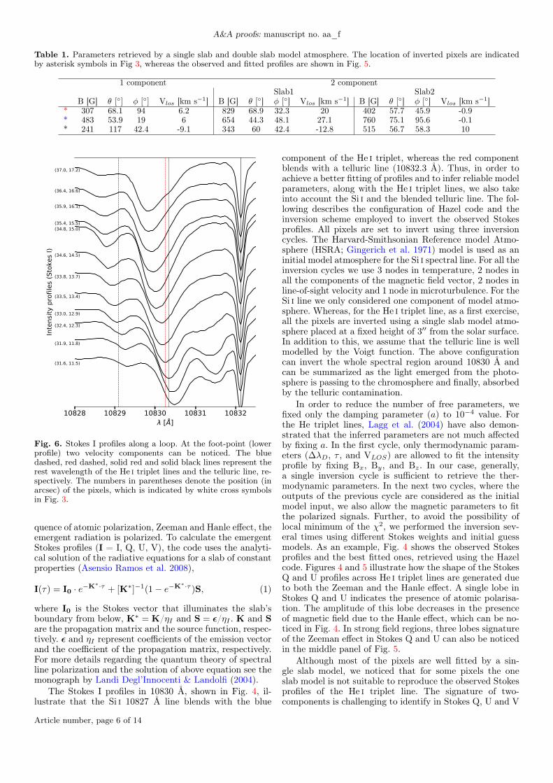
Fig. 6. Stokes I profiles along a loop. At the foot-point (lowerprofile) two velocity components can be noticed. The bluedashed, red dashed, solid red and solid black lines represent therest wavelength of the He i triplet lines and the telluric line, re-spectively. The numbers in parentheses denote the position (inarcsec) of the pixels, which is indicated by white cross symbolsin Fig. 3.

quence of atomic polarization, Zeeman and Hanle effect, theemergent radiation is polarized. To calculate the emergentStokes profiles (I = I, Q, U, V), the code uses the analyti-cal solution of the radiative equations for a slab of constantproperties (Asensio Ramos et al. 2008),

I(τ) = I0 · e−K∗·τ + [K∗]−1(1− e−K

∗·τ )S, (1)

where I0 is the Stokes vector that illuminates the slab’sboundary from below, K∗ = K/ηI and S = ε/ηI . K and Sare the propagation matrix and the source function, respec-tively. ε and ηI represent coefficients of the emission vectorand the coefficient of the propagation matrix, respectively.For more details regarding the quantum theory of spectralline polarization and the solution of above equation see themonograph by Landi Degl’Innocenti & Landolfi (2004).

The Stokes I profiles in 10830 Å, shown in Fig. 4, il-lustrate that the Si i 10827 Å line blends with the blue

component of the He i triplet, whereas the red componentblends with a telluric line (10832.3 Å). Thus, in order toachieve a better fitting of profiles and to infer reliable modelparameters, along with the He i triplet lines, we also takeinto account the Si i and the blended telluric line. The fol-lowing describes the configuration of Hazel code and theinversion scheme employed to invert the observed Stokesprofiles. All pixels are set to invert using three inversioncycles. The Harvard-Smithsonian Reference model Atmo-sphere (HSRA; Gingerich et al. 1971) model is used as aninitial model atmosphere for the Si i spectral line. For all theinversion cycles we use 3 nodes in temperature, 2 nodes inall the components of the magnetic field vector, 2 nodes inline-of-sight velocity and 1 node in microturbulence. For theSi i line we only considered one component of model atmo-sphere. Whereas, for the He i triplet line, as a first exercise,all the pixels are inverted using a single slab model atmo-sphere placed at a fixed height of 3′′ from the solar surface.In addition to this, we assume that the telluric line is wellmodelled by the Voigt function. The above configurationcan invert the whole spectral region around 10830 Å andcan be summarized as the light emerged from the photo-sphere is passing to the chromosphere and finally, absorbedby the telluric contamination.

In order to reduce the number of free parameters, wefixed only the damping parameter (a) to 10−4 value. Forthe He triplet lines, Lagg et al. (2004) have also demon-strated that the inferred parameters are not much affectedby fixing a. In the first cycle, only thermodynamic param-eters (∆λD, τ , and VLOS) are allowed to fit the intensityprofile by fixing Bx, By, and Bz. In our case, generally,a single inversion cycle is sufficient to retrieve the ther-modynamic parameters. In the next two cycles, where theoutputs of the previous cycle are considered as the initialmodel input, we also allow the magnetic parameters to fitthe polarized signals. Further, to avoid the possibility oflocal minimum of the χ2, we performed the inversion sev-eral times using different Stokes weights and initial guessmodels. As an example, Fig. 4 shows the observed Stokesprofiles and the best fitted ones, retrieved using the Hazelcode. Figures 4 and 5 illustrate how the shape of the StokesQ and U profiles across He i triplet lines are generated dueto both the Zeeman and the Hanle effect. A single lobe inStokes Q and U indicates the presence of atomic polarisa-tion. The amplitude of this lobe decreases in the presenceof magnetic field due to the Hanle effect, which can be no-ticed in Fig. 4. In strong field regions, three lobes signatureof the Zeeman effect in Stokes Q and U can also be noticedin the middle panel of Fig. 5.

Although most of the pixels are well fitted by a sin-gle slab model, we noticed that for some pixels the oneslab model is not suitable to reproduce the observed Stokesprofiles of the He i triplet line. The signature of two-components is challenging to identify in Stokes Q, U and V



due to low signal-to-noise ratio and their complex shapes.Nevertheless, they can be identified in the Stokes I profiles,as shown in Fig. 5 & 6. Generally, the two components havefast and slow velocities. As an example, Fig. 6 demonstratesthe appearance of single and double velocity components inthe Stokes I profile, one of them (the slow component) islocated close to the rest wavelength. We identify these pix-els using a threshold value of χ2, obtained after fitting theStokes I profiles using one and two components of model at-mosphere. They are mainly located near the foot-points ofloops or near the location of mixed bipolar fields. For thesepixels, we take into account the two slab model atmosphere.

In the Hazel code, two model atmospheres can be com-bined with the filling factor or as a stacked atmospheres. Inthe latter case two slab models are placed on top of eachother, whereas in the former case they are combined with afilling factor in a single pixel. It has been demonstrated thatin a FER various magnetic loops carrying helium plasmacan appear at different heights (Solanki et al. 2003; Xu, Z.et al. 2010). Under this scenario, the stacking approach canbe more realistic. Thus, in order to fit the two-componentsprofiles we considered stacking approach instead of the fill-ing factor. We placed the first (slab1) and the second slab(slab2) at the height of 2′′ and 3′′ from the solar surface,respectively. In this configuration, the light coming fromphotosphere first pass through slab1, then slab2 and finallyis absorbed by the Earth’s atmosphere (see also Eq. 4 inLibbrecht et al. 2017). As an example, the observed andbest fitted profiles are shown in Fig. 5. It also shows that asingle slab model is unable to fit the observed Stokes pro-files, however, using two slab model a reasonably good fitscan be achieved. For the selected pixels, the inferred pa-rameters using a single and double slab models are listedin Table 1. The retrieved atmospheric parameters of FERin the photosphere and chromosphere are shown in Fig. 7.After the inversion of full FOV, the next step is to removethe ambiguity in the retrieved azimuthal angle, which isdiscussed in the following section.

3.3. Ambiguity resolution

As mentioned above, at the photospheric height the trans-verse component of magnetic field vector is affected by well-known 180◦ azimuth ambiguity, which can be resolved usingdifferent available methods. In addition to this, the chromo-spheric azimuthal map inferred from Hazel can have mul-tiple possible solutions, induced by both the Zeeman andthe Hanle effects. These solutions depend on the specificregime of the magnetic field and on the scattering geome-try of the FOV (Schad et al. 2015; Díaz Baso et al. 2019).The number of solutions can go up to four (or up to eight ifthe Stokes V signal is under the noise or not given), whichcan be resolved using different approaches provided by var-ious authors (Solanki et al. 2003; Orozco Suárez et al. 2014;Schad et al. 2015; Martínez González et al. 2015).

To resolve the ambiguity in the He i triplet line we haveused the azimuth angle of the photospheric extrapolationsat a particular height as an initial estimation for our inver-sion code. This height is estimated by comparing the pho-tospheric extrapolated magnetic field strength (at differentheights) with the inferred chromospheric magnetic field. Af-ter comparison, we find that the two maps show maximumsimilarity around ∼2 Mm from the solar surface. Then, us-ing only the direction (azimuth angle, say φex) of the ex-

trapolated field lines (at ∼2 Mm) in initial guess model,we again invert the Stokes profiles. During inversion, theazimuth angles are allowed to vary in a range (φex±20◦) sothat the solution lie close to φex. Then, a visual inspectionwas also performed between the photospheric and chromo-spheric magnetograms, which reveals an overall good agree-ment (see Fig. 8 & 9). The obtained similarity suggests thatthe ambiguity resolution for He line is reliable. Note thatthe chromospheric maps shown in Fig. 7 and 8 are obtainedusing a single slab. Subsequently, the ambiguity correctedinverted maps, both for the photosphere and the chromo-sphere, are analyzed in this study.

4. Non-force free extrapolations

The plasma β parameter, which is the ratio of thermal tomagnetic pressure, can be of the order of unity in the pho-tosphere (Gary 2001). This indicates that the plasma in thephotosphere can be in a non-force free state. Thus, in thephotosphere, the retrieved current density and magnetic en-ergy in force-free extrapolations would not be reliable (Pe-ter et al. 2015). In order to understand the magnetic fieldtopology more correctly in FER, we modelled the magneticfield using non-force free field extrapolations (NFFF; Hu &Dasgupta 2008; Hu et al. 2010). The NFFF code is basedon the principle of minimum dissipation rate (MDR), whichis derived from a variational problem (Shaikh et al. 2008).Although the full MDR-based approach requires successivetwo layers of vector magnetograph measurements on thesolar surface, the same code can be modified for the sin-gle layer as demonstrated by Hu et al. (2010). This codeconstructs the magnetic field lines as the superposition oftwo linear force free fields (LFFFs) and one potential field,B = B1 + B2 + B3, where each Bi (i = 1, 2, 3) obeys thefollowing equations,

∇×B = αB; ∇ ·B = 0, (2)

here α, the so-called force-free parameter, is a function ofspace. Without a loss of generality, we can set one of thethree sub-fields (say, B1) to be potential by choosing α1

=0. While other non-potential pair satisfies, α2 6= α3 6= 0.Then, the optimal pair (α2, α3) is obtained by minimizingthe following quantity,

En =

∑Mi=1 |Bt,i − bt,i|∑M

i=1 |Bt,i|, (3)

where M represents the total number of grid points on thetransverse plane. Further, bt and Bt are the computed andmeasured transverse magnetic field vectors on the bottomboundary, respectively. Further details of the code and itsapplication to the solar active regions are given in Hu &Dasgupta (2008) (see also Hu et al. 2010)

4.1. Extrapolation using photospheric & chromosphericmagnetogram

In this section we describe the extrapolations of magneticfield lines using the magnetograms observed in the pho-tosphere and the chromosphere. We first employ the pho-tospheric vector magnetogram, retrieved by inverting theSi I 10827 line using M-E approximation, as the lower



0

5

10

15

20

25

30

Photosphere, Si I line Chromosphere, He I line

0

5

10

15

20

25

30

AB

0 10 20 30 40 50 60X [arcsec]

0

5

10

15

20

25

30

Y [a

rcse

c]

0 10 20 30 40 50 60

0.7

0.8

0.9

1.0

1.1

Inte

nsity

[I/I Q

S]

1.0

0.5

0.0

0.5

1.0

B z [k

G]

4

2

0

2

4LO

S ve

locit

y [k

m/s

ec]

0.6

0.7

0.8

0.9

Inte

nsity

[I/I c

]

0.3

0.2

0.1

0.0

0.1

0.2

0.3

B z [k

G]

20

10

0

10

20

LOS

velo

city

[km

/sec

]

Fig. 7. Left panel: inferred photospheric parameters using M-E inversion of Si I line. Right panel: inferred parameters obtainedby inverting He triplet lines using Hazel code. The magenta and black closed contours in each map represent the negativeand positive polarity of the magnetic field observed in the photosphere, respectively. Square boxes (A and B) indicatethe location of mixed polarity region.

0

10

20

30

[arc

sec]

0 10 20 30 40 50 60[arcsec]

0

10

20

30

[arc

sec]

0.00

0.25

0.50

0.75

1.00

1.25

Fiel

d st

reng

th [k

G]

50

100

150

Incli

natio

n an

gle

[°]

Fig. 8. Top: field strength retrieved by inverting He I tripletline. Bottom: inclination angle (in background) and hor-izontal magnetic field vectors are shown as black arrows.The closed white and magneta contours represent negativeand positive polarities in FOV at the photospheric level.

boundary condition for NFFF extrapolations. The compu-tation are performed in a box of 226 × 125 × 125 gridpoints in the x, y, and z directions, respectively. The dis-tance between two grid points in the horizontal and ver-tical directions is 0′′.27 (∼ 200 km). For the photosphericextrapolation the obtained En value is 0.07, suggesting theobserved and the extrapolated magnetograms at the photo-spheric level (z = 0) are remarkably similar. As an exampleof extrapolations starting from the photosphere, Fig. 9 (toppanel; in background) shows the observed Bz component ofthe photospheric magnetic field, whereas the middle andbottom panels depict the extrapolated Bz components ofthe constructed magnetic field using the NFFF at differentheights. In each panel, the arrows represent the direction ofmagnetic field vector, where their length is proportional tothe horizontal field strength. This figure also demonstratesthat for the higher regions the magnetic field strength de-creases and the field vector becomes smoother, which is gen-erally observed in extrapolations. The similarity betweenthe observed and extrapolated horizontal magnetic field isshown in Fig. 10. In this figure, blue arrows represent theobserved horizontal magnetic field derived from the inver-sion of Si i line, whereas orange arrows represent the hori-zontal magnetic field field obtained from extrapolations atthe photospheric boundary (z = 0). It is evident from thefigure that the observed and computed extrapolations are



0 10 20 30 40 50 600

5

10

15

20

25

30

Observed

0 10 20 30 40 50 600

5

10

15

20

25

30

Extrapolated, height: 0.97 Mm

0 10 20 30 40 50 60X [arcsec]

0

5

10

15

20

25

30

Y [a

rcse

c]

Extrapolated, height: 2.14 Mm

1.00

0.75

0.50

0.25

0.00

0.25

0.50

0.75

1.00

B z [k

G]0.8

0.6

0.4

0.2

0.0

0.2

0.4

0.6

0.8

B z [k

G]

0.4

0.2

0.0

0.2

0.4

B z [k

G]

Fig. 9. Top panel: The observed Bz components of the pho-tospheric magnetic field derived from the Milne-Eddington in-version of Si I line. Middle and bottom panels: Bz componentsof the photospheric magnetic field constructed using the NFFFextrapolation at different heights. The arrows show the orienta-tion of magnetic field vector, where their length is proportionalto the horizontal field strength.

remarkably similar at the lower boundary (z = 0), yieldinga linear Pearson correlation coefficient value of 0.97. Thiscomparison also ensure us that for the Si i line the ambigu-ity correction is reliable.

Although various authors have used extrapolationsstarting from photospheric magnetogram, there are onlyfew studies performed to understand the magnetic topol-ogy using the chromospheric magnetogram as lower bound-ary condition. Recently, using the photospheric and thechromospheric magnetograms as lower boundary condition,two independent NLFFF extrapolations were performed byYelles Chaouche et al. (2012) to understand the magneticfield topology of an active region filament. In addition tophotospheric extrapolation, we also performed independentextrapolations using a chromospheric vector magnetogram,which is inferred by inverting the helium triplet line, aslower boundary condition. We use the same computationaldomain as described above for the photospheric extrapola-tions. The En value for this extrapolation was 0.56. Thehigher value in this case as compared to the photosphericfield is expected as the field strength is weaker in the chro-mosphere and the uncertainities in the transverse field are

0 10 20 30 40 50 60X [arcsec]

0

5

10

15

20

25

30

35

Y [a

rcse

c]

NFFFobs.

Fig. 10. Comparison between the observed and extrapolatedhorizontal magnetic field. Blue arrows represent the observedhorizontal magnetic field derived using Si I line, whereas or-ange arrows represent the horizontal magnetic field ob-tained from extrapolations at the photospheric boundary(z = 0).

larger. The observed magnetogram is relatively small andnot isolated from the active region. So the region is far fromthe flux-balance condition, which is one of the assumptionsused in the extrapolations. Therefore, the extrapolated re-sults near the boundary can render inappropriate topologyof field lines. Thus, we mainly consider the region a few arc-seconds away from the FOV boundaries. The extrapolatedfield lines computed using the observed chromospheric mag-netic field as lower boundary condition are shown in Fig. 11.

5. Results

5.1. Magnetic field in the photosphere and chromosphere

The retrieved magnetic parameters in the FER, using theSi i line, exhibit a complex magnetic structure in the photo-sphere. The Bz component of magnetic field in photosphereillustrates that there are a few magnetic bipolar features(MBFs) in FER, two of them are highlighted in box A & B(depicted in Fig. 7). The polarity of MBFs close to a pore isopposite to the polarity of pore itself. In contrast to the pho-tospheric structure, the magnetic field in the chromosphereis relatively smooth and exhibits no signature of MBFs. Thelatter suggests that the MBFs features are more prominentin the photosphere rather than the chromosphere, which isconsistent with results from previous studies (Bernasconiet al. 2002; Solanki et al. 2003; Xu, Z. et al. 2010) Further-more, the magnetic field inferred in the photosphere and inthe chromosphere displays a weak and horizontal magneticfield in the FER. However, in the photosphere, relativelystronger and vertical magnetic fields are located in pores(∼1300 G) and in MBFs (∼800 G), whereas in the vicin-ity of FER it varies from 350 G to 600 G. Generally, inthe solar atmosphere, the magnetic field strength decreaseswith height. For instance, the mean field strength value ofa pore (∼1350 G) observed in the photosphere (located atX = 30′′, Y = 7′′) drops to 880 G in the chromosphere.Whereas the magnetic field value ranging from 100 to 400G in FER decreases by a factor of ∼0.3–0.6 compared tothe photosphere. If the average distance between the Si i



and He i formation heights is assumed as 1000–1500 km(Schmidt et al. 1994; Bloomfield et al. 2007; Xu, Z. et al.2010; Joshi et al. 2016), then the vertical gradient (∆B/∆z)in the FER turns out to be ∼0.2 G km−1, which is consis-tent with the values presented by different authors (Xu, Z.et al. 2010; Joshi et al. 2016).

5.2. LOS Velocity in photosphere and chromosphere

The inferred LOS velocity in the photosphere and chro-mosphere are shown in Fig. 7. In the photosphere, be-tween the opposite polarity pores or around the mixed-polarity regions the plasma show upflows and downflows.These flows demonstrate the expansion of the FER in thephotosphere when the pores push through the surroundingplasma. Downflows (up to 3.3 km s−1) are generally locatednear the pores of positive polarity, whereas upflows (up to2.2 km s−1) are located near the negative pore or nega-tive polarity region. In contrast to the photosphere, LOSvelocities in the upper chromosphere are relatively smooth.Near the foot-points of the elongated dark loops, connect-ing pores of opposite polarities, we found strong downflows(reaching supersonic velocities of 40 km/s), whereas strongupflows (of 22 km/s) are observed near the middle part ofthe loop.

As an example, the intensity profiles of the He tripletline along a dark featured loop are shown in Fig. 6,where the values in parentheses denote the selected posi-tion of the profiles. The top profile represent the loop apex,whereas the bottom profile represent the loop foot-point.The loop apex is strongly blueshifted (upflows). Moreover,this blueshift gradually shifts towards redshift (downflows)as a function of decreasing loop height. Near the footpointsthe profiles are strongly redshifted showing two velocitycomponents. The presence of two components of velocitynear the location of loop foot-points are also observed byLagg et al. (2007); Xu, Z. et al. (2010); González Manriqueet al. (2018). The strong upflows near the tops of freshlyemerged loops suggests that they carry cool material to theupper atmosphere, which is not yet heated to high temper-ature. Also strong downflows near the foot-points suggestthat the loop is still rising and chromospheric cool gas isdraining through the loop legs, which is consistent with theinterpretation from previous studies (Schmidt et al. 2000;Solanki et al. 2003; Xu, Z. et al. 2010; González Manriqueet al. 2018).

The overall chromospheric velocity map is remarkablydifferent from the photospheric velocity map. However,in contrast to Solanki et al. (2003); Lagg et al. (2007);González Manrique et al. (2018), we observed photosphericdownflows near the location of strong chromospheric down-flows. The maximum photospheric downflows observed atthese location is 3.3 km s−1, which is around twice the valuereported by Xu, Z. et al. (2010).

5.3. Magnetic field topology and extrapolated field lines

In addition to the reconstruction technique described bySolanki et al. (2003), the field lines can also be recon-structed using extrapolation techniques as demonstrated inWiegelmann et al. (2005). Therefore, in order to understandthe magnetic field topology in FER, we also reconstructedthe magnetic field lines using extrapolation approximations.

The three dimensional view of photospheric/chromosphericextrapolated field lines in the FER are presented in Fig. 11.Although open and closed field lines are present in the FOV,for clarity we depict only selected closed field lines. The fig-ure demonstrates that a normal magnetic field configura-tion is obtained, where the field lines start from a positivepolarity and stop near a negative polarity regions. From avisual inspection we note that almost all closed extrapo-lated field lines are parallel to the elongated dark features(see also Leenaarts et al. 2015 for the relation between Hαfibrils and the magnetic field lines in a three-dimensionalMHD simulation of a network region).

Using the photospheric extrapolations we have esti-mated the average formation height of the He line in theFER. We first compared the magnetic field strength in thephotospheric extrapolation cube at various heights with theinferred chromospheric one. We found that they show max-imum correlation around ∼1.5 Mm. If we assume that theaveraged formation height of the Si i line in a FER is 0.5 Mmfrom the solar surface (τ = 1; Bard & Carlsson 2008), then,the averaged formation height of the He i turns out to be2 Mm (1.5 Mm + the formation height of the Si i line) fromthe solar surface.

Noticeably, many field lines, reconstructed using pho-tospheric and chromospheric extrapolations, start and endaround same locations. Under normal field configurationsthe foot-points of field lines seen in the photosphere and thechromosphere should lie around the same polarity regions,which is supported by our extrapolations. The maximumheight of loops reconstructed using photospheric extrapola-tion is 10.5 Mm above the solar surface with the foot-pointseparation of 16 Mm. Furthermore, as shown in Fig. 11,there are several small loops connecting pores to nearbymagnetic structures of opposite polarity. For instance, oneof the small loops have a footpoint separation of 5 Mm andis ∼2 Mm high.

On the other hand, the magnetic loops reconstructed us-ing the chromospheric extrapolations exhibit similar topol-ogy of field lines. They show that the maximum height ofa reconstructed loop along an AFS is around 8.4 Mm (or6.4 Mm from the chromospheric height) with the foot-pointseparation of 16 Mm at the chromospheric height. In ourcase the extrapolated loops are comparable to the mag-netic loops reconstructed by Solanki et al. (2003). Theyreconstructed loops with a foot-point separation of 20 Mmand 10 Mm high. In addition to this, using the same ap-proach demonstrated by Solanki et al. (2003), in a differentFER, Xu, Z. et al. (2010) have also reconstructed loops of4–4.5 Mm high from the solar surface, which is consistentwith the present study. Since we analyzed only limited FOVof FER, the higher loops may exist in the full FER. Fur-ther, the loop height heavily depends on strength of Bz,which may vary from one FER to another.

The photospheric extrapolations reveal that strong elec-tric currents form around mixed polarity regions. They nor-mally appear at the locations of strong magnetic field gra-dient. The squashing factor (Q), generally used to quantifythis gradient, shows the most probable location of mag-netic reconnections to occur. Therefore, we also calculatethe three-dimensional Q maps using the method of Liuet al. (2016). As an example, we show top and obliqueview of Q map at the location of a mixed polarity region(box B in Fig. 7) in Fig. 12, which are generated usingthe photospheric extrapolations. We observe that intense



Fig. 11. Three dimensional view of magnetic field lines. Left panels: the extrapolated field lines computed using the observedphotospheric magnetic field as lower boundary condition (top panel: lateral view, bottom panel: top view). In background Bz

component of magnetic field strength is shown. Right panels: the extrapolated field lines computed using the observed chromosphericmagnetic field as lower boundary condition (top panel: lateral view, bottom panel: top view). In background the intensity imageshows He absorption features along the loops, closed black and white contours represent the locations of photospheric positive andnegative polarities, respectively.

Fig. 12. Top (oblique view) and bottom (top view) panels dis-play the squashing factor around a mixed polarity regions indi-cated by box B in Fig. 7. In background black and white repre-sent the locations of positive and negative polarity in the photo-sphere. The closed field lines connecting opposite polarities areshown in different colors.

brightening in AIA/SDO 1600 and 1700 Å maps are as-sociated with large Q values, which could be EBs or UVburst (Pariat et al. 2004; Vissers et al. 2015; Young et al.2018). Unfortunately, to confirm these features as EBs orUV burst we did not have much information from otherspectral lines. It is evident from the Fig. 12 that large Qvalues are located on the photospheric inversion line, alsoknown as bald patches (Titov et al. 1993), and they lie inregion of 1 – 1.6 Mm high from the solar surface. On theother hand, using chromospheric extrapolations we did notobserve strong currents and signatures of magnetic recon-

Solar surface

P1+ P2 -+- -

Downfl

ows D

ownflow

s

Upflows

*< He I >

Fig. 13. A sketch of the magnetic field configuration in a FERbased on the two layer extrapolations. The ’+’ and ’-’ sym-bols represent positive and negative polarity on solar surface,respectively. The gray area outlined by dashed lines representthe average formation height of He i layer. An AFS connectingtwo pores (P1 and P2) of opposite polarity is represented by ablack closed loop. Arrows indicate the upflows and downflowsof plasma along an AFS as observed in the He triplet line. Theasterisk symbol indicates the plausible location of magnetic re-connection near a mixed polarity region.

nection in the chromosphere. The analysis of the magnetictopology and Q maps suggests that the observed bright-ening are generated through magnetic reconnection in thelower chromosphere or upper photosphere, which is consis-tent with the previous suggestions (Georgoulis et al. 2002;Pariat et al. 2004; Vissers et al. 2013; de la Cruz Rodríguezet al. 2015; Toriumi et al. 2017; Tian et al. 2018; Visserset al. 2019).

6. Discussion and conclusions

In this article we have analyzed spectropolarimetric obser-vations of a young FER located close to the solar limb.We have analyzed the magnetic and kinematic nature of a



FER in the photosphere and chromosphere using the Si i10827 Å and He i 10830 Å triplet lines. In order to retrievethe physical properties of solar atmosphere, the Si i line isinverted using Milne-Eddington atmosphere, whereas He itriplet line is inverted using the Hazel inversion code by con-sidering a joint action of the Hanle effect and the Zeemaneffect.

Through spectropolarimetric analysis of the Si i line weobserved a complex magnetic structure showing a few mag-netic bipolar elements near the vicinity of FER. In the pho-tosphere, the magnetic field is weak (350 – 600 G) andhorizontal around the middle part of FER. However, it be-comes relatively strong (∼1000 G) and more vertical nearthe pores. The obtained overall features at the photosphericlevel are consistent with previous results (Solanki et al.2003; Lagg et al. 2004; Xu, Z. et al. 2010). Our analysis ofthe He i triplet line shows a smooth variation of the mag-netic field vector (ranging from 100 G to 400 G) and ve-locity across FER. Furthermore, we find supersonic down-flows of ∼40 km s−1 near the foot points of loops connect-ing two pores of opposite polarity, while a strong upflowsof ∼22 km s−1 near the middle part of loops. Recently,González Manrique et al. (2018) studied the evolution ofan AFS in a FER using 64 minutes of observations. Us-ing He i 10830 intensity profiles, they measured strong up-flows (near the central part) and downflows (near the foot-points) in loops. During 30 minutes of lifetime, the upflowsdecreases gradually whereas the downflows increases in themiddle stage and again decreases at the later stage. Finally,the AFS vanishes when downflows drops to zero. Based ontheir observations, the strong upflows in the present studyindicates that the loops are young and carry cool materialto the upper atmosphere, which is also evident from thestrong He i triplet line absorption along the emerged loops.

In contrast to Lagg et al. (2007); González Manriqueet al. (2018), at the location of the supersonic downflowsin the chromosphere, we observed downflows of ∼3 km s−1in the photosphere. In addition to this, Xu, Z. et al. (2010)have also reported photospheric downflows of 1.5 km s−1below regions with chromospheric downflows. The observedstrong photospheric downflows could be a consequence ofatmospheric disturbances caused by the supersonic down-flowing material along the loop foot-points. Moreover, incontrast to Lagg et al. (2007), no signs of emission in theHe i line observed in our analysis, which indicates that thetransition of downflowing material from supersonic to sonicvelocities lie below the He i line formation.

To understand the magnetic field topology in FER, weemployed NFFF extrapolations starting from our photo-spheric and chromospheric magnetic field measurements.A normal magnetic configuration (connecting positive tonegative polarity regions) is observed above the FER. Weobserved that there are several magnetic loops of smalland large scales, where small-scale loops lie beneath thelarge-scale loops forming magnetic canopies of various size.The magnetic loops reconstructed using photospheric ex-trapolations along an AFS have a maximum height of10.5 Mm with the foot-points separation of 19 Mm, whereasthe loops reconstructed using chromospheric extrapolationsare around 8.4 Mm high with the foot-point separation of16 Mm.They are almost aligned along the He i line absorp-tion features, which is consistent with the previous find-ings. However, in the lower chromosphere, the observationsin Ca ii 8542 Å have revealed that the magnetic vectors

are mostly directed along the dark features or fibrils, butnot always (de la Cruz Rodríguez & Socas-Navarro 2011;Asensio Ramos et al. 2017), which could be an effect of theCa ii 8542 Å line forming deeper in the atmosphere.

The small-scale heating events (EBs or UV bursts) andenergy release at different heights have been observed abovethe FER. Our analysis suggests that the appearance ofthese events, or in general the heating of upper layers in thesolar atmosphere, is likely due to the magnetic reconnectionbetween the magnetic loops of opposite directions. We alsoobserved that the intense small-scale bright features in AIA1600 and 1700 Å are associated with large Q values, indicat-ing that they are energized by small scale magnetic recon-nections, which is consistent with the previous suggestions.In our analysis, the magnetic field strength is horizontal inthe vicinity of FER, but no significant brightening observedin the upper chromosphere using He i triplet line. However,in a recent analysis of FER using multi-line observations athigh spatial and temporal resolution, Leenaarts et al. (2018)reported that the heating rate in the low chromosphere cor-relates with the strength of the horizontal magnetic field.The role of magnetic field vector in the chromospheric heat-ing is still unclear, thus more investigations of FER or activeregion using multi-line observations are required.

Based on the analysis of spectropolarimetric data attwo layers, the magnetic field configuration of a FER issketched in Fig. 13. This cartoon also illustrates the rear-rangement of magnetic field lines during reconnection neara mixed polarity region, which lie in the lower chromosphereor upper photosphere. The overall magnetic topology in theFER shown here is in agreement with the previous findings(Solanki et al. 2003; Xu, Z. et al. 2010; Toriumi et al. 2017;González Manrique et al. 2018) and supports the theoret-ical AFS models. In future we would investigate the mag-netic configuration of a FER and the presence of currentsheets around the loops using two boundary conditions (atdifferent layers) in a single extrapolation. Moreover, multi-line observations at high-spatial and temporal resolutionrequired to understand the observational consequences ofFER in different layers. The advent of new generation solartelescopes, such as, the Daniel K. Inouye Solar Telescope(DKIST; Tritschler et al. 2015) and the European SolarTelescope (EST; Matthews et al. 2016) would be crucial inthis regard.Acknowledgements. We would like to thank the anonymous refereefor the comments and suggestions. The 1.5 m GREGOR solar tele-scope was built by a German consortium under the leadership of theKiepenheuer Institut für Sonnenphysik in Freiburg with the LeibnizInstitut für Astrophysik Potsdam, the Institut für Astrophysik Göt-tingen, and the Max-Planck Institut für Sonnensystemforschung inGöttingen as partners, and with contributions by the Instituto de As-trofísica de Canarias and the Astronomical Institute of the Academyof Sciences of the Czech Republic. The observing time at GREGORwas provided by the Trans-National Access and Service Programme ofthe SOLARNET project, funded by the European Commission’s 7thFramework Programme under grant agreement No. 312495. JdlCR issupported by grants from the Swedish Research Council (2015-03994),the Swedish National Space Board (128/15) and the Swedish CivilContingencies Agency (MSB). This project has received funding fromthe European Research Council (ERC) under the European Union’sHorizon 2020 research and innovation programme (SUNMAG, grantagreement 759548). The Institute for Solar Physics is supported bya grant for research infrastructures of national importance from theSwedish Research Council (registration number 2017-00625). AP ac-knowledges partial support of NASA grant 80NSSC17K0016 and NSFaward AGS-1650854. AAR acknowledges financial support from theSpanish Ministerio de Ciencia, Innovación y Universidades throughproject PGC2018-102108-B-I00 and FEDER funds. We acknowledge



the use of the visualization software VAPOR (www.vapor.ucar.edu)for generating relevant graphics. Data and images are courtesy ofNASA/SDO and the HMI and AIA science teams. This research hasmade use of NASA’s Astrophysics Data System. We acknowledge thecommunity effort devoted to the development of the following open-source packages that were used in this work: numpy (numpy.org),matplotlib (matplotlib.org) and sunpy (sunpy.org).

ReferencesAndretta, V. & Jones, H. P. 1997, ApJ, 489, 375

Asensio Ramos, A., de la Cruz Rodríguez, J., Martínez González,M. J., & Socas-Navarro, H. 2017, A&A, 599, A133

Asensio Ramos, A., Trujillo Bueno, J., & Land i Degl’Innocenti, E.2008, ApJ, 683, 542

Auer, L. H., Heasley, J. N., & House, L. L. 1977, Sol. Phys., 55, 47

Bard, S. & Carlsson, M. 2008, ApJ, 682, 1376

Bernasconi, P. N., Rust, D. M., Georgoulis, M. K., & Labonte, B. J.2002, Sol. Phys., 209, 119

Bloomfield, D. S., Lagg, A., & Solanki, S. K. 2007, ApJ, 671, 1005

Bobra, M. G., Sun, X., Hoeksema, J. T., et al. 2014, Sol. Phys., 289,3549

Bommier, V., Sahal-Brechot, S., & Leroy, J. L. 1981, A&A, 100, 231

Bruzek, A. 1967, Sol. Phys., 2, 451

Caligari, P., Moreno-Insertis, F., & Schussler, M. 1995, ApJ, 441, 886

Casini, R., López Ariste, A., Tomczyk, S., & Lites, B. W. 2003, ApJ,598, L67

Centeno, R., Trujillo Bueno, J., & Asensio Ramos, A. 2010, ApJ, 708,1579

Centeno, R., Trujillo Bueno, J., Uitenbroek, H., & Collados, M. 2008,ApJ, 677, 742

Cheung, M. C. M. & Isobe, H. 2014, Living Reviews in Solar Physics,11, 3

Chou, D.-Y. 1993, in Astronomical Society of the Pacific ConferenceSeries, Vol. 46, IAU Colloq. 141: The Magnetic and Velocity Fieldsof Solar Active Regions, ed. H. Zirin, G. Ai, & H. Wang, 471–478

Collados, M., López, R., Páez, E., et al. 2012, AstronomischeNachrichten, 333, 872

Collados, M. V. 2003, in Society of Photo-Optical InstrumentationEngineers (SPIE) Conference Series, Vol. 4843, Proc. SPIE, ed.S. Fineschi, 55–65

de la Cruz Rodríguez, J., Hansteen, V., Bellot-Rubio, L., & Ortiz, A.2015, ApJ, 810, 145

de la Cruz Rodríguez, J. & Socas-Navarro, H. 2011, A&A, 527, L8

del Toro Iniesta, J. C. 2003, Introduction to Spectropolarimetry, 244

Díaz Baso, C. J., Martínez González, M. J., & Asensio Ramos, A.2019, A&A, 625, A128

Fan, Y. 2004, Living Reviews in Solar Physics, 1, 1

Gary, G. A. 2001, Solar Physics, 203, 71

Gary, G. A. & Hagyard, M. J. 1990, Sol. Phys., 126, 21

Georgoulis, M. K., Rust, D. M., Bernasconi, P. N., & Schmieder, B.2002, ApJ, 575, 506

Gingerich, O., Noyes, R. W., Kalkofen, W., & Cuny, Y. 1971,Sol. Phys., 18, 347

Goldberg, L. 1939, ApJ, 89, 673

González Manrique, S. J., Kuckein, C., Collados, M., et al. 2018, A&A,617, A55

Hoeksema, J. T., Liu, Y., Hayashi, K., et al. 2014, Sol. Phys., 289,3483

Hu, Q. & Dasgupta, B. 2008, Sol. Phys., 247, 87

Hu, Q., Dasgupta, B., Derosa, M. L., Büchner, J., & Gary, G. A. 2010,Journal of Atmospheric and Solar-Terrestrial Physics, 72, 219

Joshi, J., Lagg, A., Solanki, S. K., et al. 2016, A&A, 596, A8

Judge, P. G. 2009, A&A, 493, 1121

Judge, P. G., Kleint, L., & Sainz Dalda, A. 2015, ApJ, 814, 100

Kuckein, C., Centeno, R., Martínez Pillet, V., et al. 2009, A&A, 501,1113

Kuckein, C., Collados, M., & Manso Sainz, R. 2015, ApJ, 799, L25

Lagg, A., Woch, J., Krupp, N., & Solanki, S. K. 2004, A&A, 414, 1109

Lagg, A., Woch, J., Solanki, S. K., & Krupp, N. 2007, A&A, 462, 1147

Landi Degl’Innocenti, E. & Landolfi, M., eds. 2004, Astrophysics andSpace Science Library, Vol. 307, Polarization in Spectral Lines

Leenaarts, J., Carlsson, M., & Rouppe van der Voort, L. 2015, ApJ,802, 136

Leenaarts, J., de la Cruz Rodríguez, J., Danilovic, S., Scharmer, G.,& Carlsson, M. 2018, A&A, 612, A28

Leenaarts, J., Golding, T., Carlsson, M., Libbrecht, T., & Joshi, J.2016, A&A, 594, A104

Leka, K. D., Barnes, G., & Crouch, A. 2014, AMBIG: AutomatedAmbiguity-Resolution Code, Astrophysics Source Code Library

Lemen, J. R., Title, A. M., Akin, D. J., et al. 2012, Sol. Phys., 275,17

Libbrecht, T., Joshi, J., Rodríguez, J. d. l. C., Leenaarts, J., & Ramos,A. A. 2017, A&A, 598, A33

Liu, R., Kliem, B., Titov, V. S., et al. 2016, ApJ, 818, 148

López Ariste, A. & Casini, R. 2005, A&A, 436, 325

Martínez González, M. J., Asensio Ramos, A., Carroll, T. A., et al.2008, A&A, 486, 637

Martínez González, M. J., Asensio Ramos, A., Manso Sainz, R., Beck,C., & Belluzzi, L. 2012, ApJ, 759, 16

Martínez González, M. J., Sainz, R. M., Ramos, A. A., et al. 2015,The Astrophysical Journal, 802, 3

Matthews, S. A., Collados, M., Mathioudakis, M., & Erdelyi, R. 2016,in Society of Photo-Optical Instrumentation Engineers (SPIE)Conference Series, Vol. 9908, Proc. SPIE, 990809

Merenda, L., Lagg, A., & Solanki, S. K. 2011, A&A, 532, A63

Merenda, L., Trujillo Bueno, J., Landi Degl’Innocenti, E., & Collados,M. 2006, ApJ, 642, 554

Metcalf, T. R. 1994, Sol. Phys., 155, 235

Metcalf, T. R., Leka, K. D., Barnes, G., et al. 2006, Solar Physics,237, 267

Orozco Suárez, D., Asensio Ramos, A., & Trujillo Bueno, J. 2014,A&A, 566, A46

Orozco Suárez, D., Asensio Ramos, A., & Trujillo Bueno, J. 2015,ApJ, 803, L18


numpy.org

matplotlib.org

sunpy.org


Pariat, E., Aulanier, G., Schmieder, B., et al. 2004, ApJ, 614, 1099

Parker, E. N. 1955, ApJ, 121, 491

Pesnell, W. D., Thompson, B. J., & Chamberlin, P. C. 2012,Sol. Phys., 275, 3

Peter, H., Warnecke, J., Chitta, L. P., & Cameron, R. H. 2015, A&A,584, A68

Ruiz Cobo, B. & del Toro Iniesta, J. C. 1992, ApJ, 398, 375

Sasso, C., Lagg, A., & Solanki, S. K. 2014, A&A, 561, A98

Schad, T. A. 2018, ApJ, 865, 31

Schad, T. A., Penn, M. J., Lin, H., & Judge, P. G. 2016, ApJ, 833, 5

Schad, T. A., Penn, M. J., Lin, H., & Tritschler, A. 2015, Solar Physics,290, 1607

Scherrer, P. H., Schou, J., Bush, R. I., et al. 2012, Sol. Phys., 275, 207

Schmidt, W., Knoelker, M., & Westendorp Plaza, C. 1994, A&A, 287,229

Schmidt, W., Muglach, K., & Knölker, M. 2000, ApJ, 544, 567

Schmidt, W., von der Lühe, O., Volkmer, R., et al. 2012, Astronomis-che Nachrichten, 333, 796

Shaikh, D., Dasgupta, B., Zank, G. P., & Hu, Q. 2008, Physics ofPlasmas, 15, 012306

Solanki, S. K., Inhester, B., & Schüssler, M. 2006, Reports on Progressin Physics, 69, 563

Solanki, S. K., Lagg, A., Woch, J., Krupp, N., & Collados, M. 2003,Nature, 425, 692

Tian, H., Zhu, X., Peter, H., et al. 2018, ApJ, 854, 174

Tipping, M. E. 2000, The Relevance Vector Machine

Titov, V. S., Priest, E. R., & Demoulin, P. 1993, A&A, 276, 564

Toriumi, S., Katsukawa, Y., & Cheung, M. C. M. 2017, ApJ, 836, 63

Tritschler, A., Rimmele, T. R., Berukoff, S., et al. 2015, in CambridgeWorkshop on Cool Stars, Stellar Systems, and the Sun, Vol. 18,18th Cambridge Workshop on Cool Stars, Stellar Systems, and theSun, 933–944

Trujillo Bueno, J. & Asensio Ramos, A. 2007, ApJ, 655, 642

Trujillo Bueno, J., Landi Degl’Innocenti, E., Collados, M., Merenda,L., & Manso Sainz, R. 2002, Nature, 415, 403

Trujillo Bueno, J., Merenda, L., Centeno, R., Collados, M., & LandiDegl’Innocenti, E. 2005, ApJ, 619, L191

van Driel-Gesztelyi, L. & Green, L. M. 2015, Living Reviews in SolarPhysics, 12, 1

Vissers, G. J. M., de la Cruz Rodríguez, J., Libbrecht, T., et al. 2019,A&A, 627, A101

Vissers, G. J. M., Rouppe van der Voort, L. H. M., & Rutten, R. J.2013, ApJ, 774, 32

Vissers, G. J. M., Rouppe van der Voort, L. H. M., Rutten, R. J.,Carlsson, M., & De Pontieu, B. 2015, ApJ, 812, 11

Wiegelmann, T., Lagg, A., Solanki, S. K., Inhester, B., & Woch, J.2005, A&A, 433, 701

Wiegelmann, T. & Sakurai, T. 2012, Living Reviews in Solar Physics,9, 5

Wiegelmann, T., Thalmann, J. K., & Solanki, S. K. 2014, A&A Rev.,22, 78

Xu, Z., Lagg, A., & Solanki, S. K. 2010, A&A, 520, A77

Yadav, R., Mathew, S. K., & Tiwary, A. R. 2017, Sol. Phys., 292, 105

Yelles Chaouche, L., Kuckein, C., Martínez Pillet, V., & Moreno-Insertis, F. 2012, ApJ, 748, 23

Young, P. R., Tian, H., Peter, H., et al. 2018, Space Sci. Rev., 214,120

Zeeman, P. 1897, ApJ, 5, 332

Zirin, H. 1975, ApJ, 199, L63

Zwaan, C. 1985, Sol. Phys., 100, 397


Documents

regioninthesolaratmosphere - arXiv