Regional models of potential evaporation and reference ...engineering.tufts.edu/cee/people/vogel/documents/regional... · Regional models of potential evaporation and reference evapotranspiration

Journal of Hydrology

ELSEVIER Journal of Hydrology 184 (1996) 337-354

Regional models of potential evaporation and reference evapotranspiration for the northeast USA

Neil M. Fennessey a'*, Richard M. Vogel b

aDepartment of Civil and Environmental Engineering, University of Massachusetts, North Dartmouth, MA 02747, USA

bDepartment of Civil and Environmental Engineering, Tufts University, Anderson Hall, Medford, MA 02155, USA

Received 22 August 1994; accepted 29 October 1995

Abstract

Multivariate regression models of average monthly reference crop evapotranspiration, Et('r), and potential evaporation, Ep(r), are developed for the northeast USA. Average monthly values of daily Et and Ep are estimated from the Penman-Monteith equation using monthly climate data from 34 National Oceanic and Atmospheric Administration (NOAA) First Order weather observatories and specific reference vegetation characteristics. The periodic seasonal behavior of Et(7" ) and Ep(r) and average monthly temperature are approximated by Fourier series functions. Regional regression relationships are then developed which relate the Et(7- ) and Ep(r) Fourier series coefficients with the average monthly temperature Fourier coefficients, station longitude and station elevation. The regional Et(z) model is shown to be an improvement over the Linacre method (Linacre, 1977, Agric. Meteorol., 18: 409-424) and the Hargreaves and Samani method (Hargreaves and Samani, 1985, Appl. Eng. Agric., 1(2): 96-99), and the regional Ep(r) model is shown to be an improvement over the Linacre method.

I. Introduction

The Penman-Montei th equation (Monteith, 1965) is an accepted method for describing reference crop evapotranspiration Et: the atmosphere's near-earth surface demand for water vapor above a well-watered reference vegetation. The primary disadvantage of the Penman-Montei th equation is its data requirements, which include net solar radiation, windspeed, dewpoint temperature, air temperature and vegetation-specific parameters.

* Corresponding author.

0022-1694/96/$15.00 Copyright © 1996 Published by Elsevier Science B.V. All rights reserved PII 0022-1694(95)02980-X

J*

* /

*

MILE

S I00

20

0 I

. ,

. i

1(10

20

0 30

0 KIL

OMET

ERS

Fig.

1.

Loc

atio

n of

the

NO

AA

Fir

st O

rder

obs

erva

tori

es.

N.M. Fennessey, R.M. Vogel~Journal of Hydrology 184 (1996) 337-354 339

These climate data are generally only available at National Oceanic and Atmospheric Administration (NOAA) First Order observatories, typically located at major metropolitan airports and staffed by trained weather observers. For example, Fig. 1 illustrates the locations of the 34 NOAA First Order observatories used in this study. In contrast, local average monthly temperature data are far more readily available from other Federal or State supported networks (over 1000 stations in New England, New York, New Jersey and Pennsylvania). As Et can only readily be estimated at First Order observatories, a method to estimate E t using local temperature and other readily available site-specific data would be useful in a broad range of water resources studies including reservoir yield and climate change impact analyses.

The first objective of this study was the development of a multivariate regional regression model which may be used to estimate Et(7"), 7" -~ 1,12, the average monthly evapotranspiration rate at any location in the northeastern USA for a reference vegetation. The second objective was to develop a similar regional model for monthly average potential evaporation, Ep(r), r = 1,12, the atmosphere's demand for water vapor above a free water surface. In this study, Et(7") is estimated for a reference grass of 12 cm height. The study concludes with a comparison of the methods developed here for estimating Et(7") and Ep(r) with other temperature-based models.

2. Reference crop evapotranspiration

Reference crop evapotranspiration is the atmosphere's near-earth surface demand for water vapor from a moist, well-watered soil completely covered by a transpiring but dry vegetation canopy. The reference vegetation has specific physical characteristics. The Penman-Monteith equation (Monteith, 1965) remains the model of choice when estimating actual evapotranspiration (see Jensen et al. (1990) and Shuttleworth (1993)).

The Penman-Monteith equation describes the vertical (one-dimensional) latent heat flUX, ~kEt:

A(Rn _ GI) + pCp[e°(z) - e(z)]

~.E t ~ ra

where • is the latent heat of vaporization, Et is the reference crop evapotranspiration, A is the gradient of the saturation vapor pressure-temperature function, R, is the net radiation, Gt is the vertical heat energy flux within the soil, P is the air density, Cp is the specific heat of the air at constant pressure, e°(z) is the saturated vapor pressure of the air measured at height z, e(z) is the vapor pressure of the air measured at height z, r, is the aerodynamic resistance to water vapor diffusion into the atmospheric boundary layer, rc is the vegetation's canopy resistance to water vapor transfer, and ',/ is the psychrometric constant. Further details associated with Eq. (1) have been described by Jensen et al. (1990), Fennessey (1994) and Fennessey and Kirshen (1994), and elsewhere.

340 N.M. Fennessey, R.M. Vogel~Journal of Hydrology 184 (1996) 337-354

2.1. Vegetation data

Several vegetation-specific variables are required by the Penman-Monteith equation. In this study, ra, the aerodynamic resistance (see, e.g. Brutsaert (1984) or Jensen et al. (1990, p. 93)) is determined by

i n ( zw -dO~ln(Zp-do ~ k, Zom / \ Zov ]

r a = r2U(zw ) (2)

where Zw and Zp are the heights of the windspeed anemometer and humidity psychrometer, respectively, do is the zero-windspeed plane displacement height, Zom is the roughness length for momentum transfer, Zov is the roughness length for vapor transfer, K is von K~rm~in's constant and U(zw) is the windspeed measured at height Zw. Eq. (2)is valid for a neutrally buoyant atmosphere (no free convection), which is a reasonable assumption for estimates of reference crop evapotranspiration at time scales of 1 day or greater.

For a reference vegetation, we use a grass of height hc = 12 cm with a canopy resistance, re, of 70 s m -1. Jensen et al. (1990) suggested do = 0.67hc, Zorn = 0.123hc, Zov = 0.1Zom and r = 0.41. Finally, we use surface albedo of 0.23, as suggested by Shuttleworth (1993), which is necessary to estimate the net radiation, Rn, in Eq. (1) (see Fennessey and Kirshen, 1994).

3. Regional regression model for reference crop evapotranspiration

Our objective was to develop a procedure for obtaining an accurate estimate of Et(r), the average monthly value of the daily reference crop evapotranspiration rate, using readily available independent variables. This would allow one to obtain good estimates of Et(r) anywhere in the northeastern USA, unlike the current situation, which only allows for good estimates of Et(7" ) in the 'local' vicinity of major metropolitan airports. Spatial interpolation of Et(7") estimates derived from NOAA observatory data is not an attractive way to estimate site-specific Et(7") because the topography of the northeast USA between adjacent stations may range from coastal plains to mountains of 1900 m or more.

3.1. Regional climate data

Estimates of the average monthly reference crop evapotranspiration using the Penman- Monteith equation were obtained using climate data from 34 NOAA First Order observatories and the procedures described by Fennessey and Kirshen (1994). The data are based upon average monthly values of the daily climate variables derived from the 'Normal' 1951-1980 record period. These long-term normal climate data are available in the Local Climatological Data Annual Summary with Comparative Data, published by the National Climatic Data Center (NCDC), Ashville, NC. The locations of these observatories are shown in Fig. 1 and listed in Table 1. These data include either observed cloud cover and/ or per cent of possible sunshine, relative humidity, windspeed and air temperature. The station air pressure was also used if it was reported. The NOAA observatories record


Table 1

NOAA First Order climate observatories

Gage Location NOAA id. Latitude Longitude Elevation

1 Portland, ME 14764 43039 ' 70o18 ' 13

2 Caribou, ME 14607 46°52 ' 68°01 ' 190 3 Concord, NH 14745 43°12 ' 71o30 ' 104 4 Mt. Washington, Gorham, NH 14755 44016 , 71018 ' 1909 5 Burlington, VT 14742 44028 ' 73009 ' 101

6 Blue Hill Obs., Milton, MA 14753 42o13 ' 71007 ' 192 7 Boston, MA 14739 42022 ' 71002 ' 5

8 Worcester, MA 94746 42o16 ' 71°52 ' 301 9 Hartford, CT 14740 41o56 ' 72°41 ' 52 10 Bridgeport, CT 94702 41010 ' 73°08 ' 2 11 Providence, RI 14765 41044 ' 71026 ' 16 12 Syracuse, NY 14771 43007 , 76007 ' 125

13 Rochester, NY 14768 43007 ' 77°40 ' 167 14 La Guardia Field, New York, NY 14732 40046 ' 73054 ' 3

15 JFK Airport, New York, NY 94789 40°39 ' 73o47 ' 4 16 Central Park, New York, NY 94728 40047 ' 73058 ' 40 17 Buffalo, NY 94728 42056 ' 78044 ' 215 18 Binghampton, NY 04725 42013 ' 75059 ' 485

19 Albany, NY 14735 42o45 ' 73°48 ' 84 20 Newark, NJ 14734 40o42 ' 74010 , 2

21 Atlantic City, NJ 93730 39027 ' 74o34 ' 20 22 Williamsport, PA 14778 41015 ' 76055 ' 160 23 Pittsburgh, PA 94823 40030 ' 80013 ' 347

24 Philadelphia, PA 13739 39053 ' 75°15 , 2 25 Erie, PA 14860 42005 ' 80011 ' 223

26 Allentown, PA 14737 40039 , 75°26 ' 118

27 Baltimore, MD 93721 39"11' 76o40 ' 45 28 Richmond, VA 13740 37030 ' 77020 ' 50 29 Roanoke, VA 13741 37019 ' 79o58 ' 350

30 Lynchburg, VA 13733 37"20' 79012 ' 281 31 Wilmington, DE 13781 39040 ' 75036 ' 23

32 National Arpt., Washington, DC 13743 38051 ' 77002 ' 3 33 Youngstown, OH 14852 41°15 ' 80040 ' 359 34 Akron, OH 14895 40°55 ' 81026 ' 368

r e l a t i v e h u m i d i t y f o u r t i m e s d a i l y a n d t he A n n u a l S u m m a r y t a b u l a t e s t he 1 9 5 1 - 1 9 8 0

a v e r a g e o f e a c h v a l u e e v e r y m o n t h . In t h i s s t u d y , t he a v e r a g e o f t h o s e f o u r d a i l y r e l a t i v e

h u m i d i t y v a l u e s w a s u s e d to e s t i m a t e a s i n g l e a v e r a g e d a i l y r e l a t i v e h u m i d i t y .

3.2. Fourier series approximation o f Et(~ r)

P e r i o d i c d a t a c a n be a p p r o x i m a t e d b y a c o n t i n u o u s F o u r i e r s e r i e s f u n c t i o n . F o r t h i s

s t u d y , w e u s e d t he F o u r i e r s e r i e s f o r m u l a t i o n r e p o r t e d b y B l o o m f i e l d ( 1 9 7 6 ) to a p p r o x -

i m a t e Et(T). T h e F o u r i e r s e r i e s a p p r o x i m a t i o n is

E t,f(7") ~-" Eta + k = l ~ a k c o s + el, s in k ~ - ) (3)


where r is the month, r = 1,12; Et,f(r) denotes the Fourier series approximation to the average monthly value of the daily reference crop evapotranspiration during the rth month; Eta is the annual average daily reference crop evapotranspiration rate; k is the summation index for the kth harmonic; m equals the total number of harmonics required to accurately approximate Et(r) derived from the Penman-Monteith equation• We determined that m = 2 harmonics results in values of Et,f(T ) which closely approximate Et(T ).

The Fourier series coefficients for the kth harmonic of Et,f(r), ak and bk, are estimated using

1 12 7rkr ak = ~r~l[Et(r)-Eta]COS( ~ - ) (4a)

1 12 • 7rkT bk=~r~l[Et(q')-Eta]Sln(-~- ) (4b)

3•3• Regional regression model for Et(r )

The near-earth surface air temperature is an indicator of the planetary boundary layer heat and moisture fluxes and the surface energy balance. Therefore, we attempted to estimate Et(7") using multivariate regression with air temperature likely to be the most important candidate independent variable. As noted by Fennessey and Kirshen (1994), equations which describe many of the individual Penman-Monteith equation variables in Eq. (1) are temperature dependent•

Regional regression equations were developed which describe the five reference crop evapotranspiration Fourier coefficients of a two harmonic form of Eq. (3): Eta, al, ba, a2 and b2. The candidate independent variables include station decimal latitude, longitude and elevation, average monthly temperature and the average annual temperature• Owing to significant intercorrelation among monthly values of temperature (range 0.932-0.997), we chose to fit a Fourier series to monthly temperatures rather than face parameter estimation difficulties associated with multicollinearity (see Hirsch et al., 1993)•

Fourier series were fitted to monthly average temperatures, T(r), 7" = 1,12, shown by

• 7rkr Zf(T) ~ Ta+k~=l[ekCOS(~)+dkSln(~--)l (5)

where Tf(r) is the Fourier series approximation of the monthly averaged daily temperature (in °C) for the rth month and Ta is the annual average daily temperature• Like Et,f(r), we limited Tf(r) to the first two harmonics, hence the five Tf(z) Fourier series coefficients are described by Ta, Cl, dl, c2 and d2 using

ra = r 2=1T(T) (6a)

1 ~ IT(,-)- Ta]cOs( ~" ) C A = 6 ~ 6 - (6b)


Table 2 Coefficients for the Eq. (7) regional regression equations required to estimate the reference crop evapotranspiration

0t Model coefficients

e0 el e2 e3 e4 65 e6 e7

Eta 1.25 0.0 0.0 0.118 0.0 0.0 0.0 0.0 al 1 . 6 2 -0.00843 0.0 -0.0860 0.191 0.0 -0.564 0.0 bl 2 . 5 9 -0.0137 0.0 -0.0318 0.0 0.269 0.0 -0.190 a2 -0.637 0 .00761 -0.000095 0.0 -0.0573 0.0374 0.404 0.0 b2 -0.708 0 .00409 -0.000131 0.0 -0.0403 -0.039 0.271 0.205

1 1 2 . 71"T

(6c)

1 12 (a'r) (6d) c2 = g r~l [T(r) - Ta]C°S T

1 12 . 71"T d2= ~r~=l[T(7-)-Ta]Sln(-~- ) (6e)

Even though the mon th ly average tempera ture values, T(r), are highly coll inear, the

corre la t ion matr ix a m o n g the five Four ier coeff ic ients o f Tf(r) are m u c h smaller , ranging

f rom 0.407 to 0.828.

Reg iona l equa t ions for dependen t var iables Eta , al, a2, bl and b2 are deve loped us ing the

i ndependen t var iables station dec imal longi tude, s ta t ion elevat ion, Ta, cl, c2, dl and d2. The

stat ion latitude is h ighly corre la ted (r = 0.920) wi th dl; hence , lat i tude was d ropped f rom

further cons idera t ion . The final regress ion equat ions take the fo rm

0 t = e 0 + e l L o n g + e2Elev + e3T a + eac 1 (7)

+ esdl + e6c2 + e7d2

where Long is the site longi tude (in dec imal degrees) , Elev is the site e levat ion (in meters) ,

and 0t denotes the dependen t var iable Eta, al , bl, a2 or b2.

Table 2 s h o w s the coeff ic ients e0 to e7 for the regional equat ions . Table 3 d o c u m e n t s the

Table 3 Student t-ratios and adjusted coefficient of determination, R 2, of the five regional regressions described by Eq. (7)

0t Student t-Ratios a R 2

e0 el e2 e3 e4 e5 e6 e7

Eta 23.53 - - 23 .02 . . . . 94.1 a 1 5.02 -2.42 - -14.68 10.95 - -5.33 - 91.8 bl 7.32 -4.33 - -9.31 - 11.67 - -3.84 83.7 a2 -4.24 6.48 -6.30 - -8.57 2.40 7.60 - 90.0 b2 -2.46 2.29 -7.86 - -2.55 -2.23 4.42 4.19 84.8

a The critical value of the t-ratio, using a 5% significance level, is/0.025,32 ~ 2.03.

344 N.M. Fennessey, R.M. Vogel/Journal of Hydrology 184 (1996) 337-354

21 • - - - Et,r (T) Mr. W a s h i n g t o n , N.H. [---] Et(~')

W o r c e s t e r , MA. 0

2

%

e--e Et,r(r) C2 Et(T)

e - - e Et,r (~") Et(~')

2

J F M A M J J A S O N D Month

Fig. 2. Comparison between Penman-Monteith estimated Et(r ) and regional regression model Et,r(~- ) reference crop evapotranspiration at three NOAA observatories.

Student t-ratio for each coefficient and each regression equation's adjusted coefficient of determination, R 2. It should be noted that R 2 cannot be computed if the intercept coefficient, eo, equals zero. All computed t-ratios in Table 3 were larger than Tcrit =/0.025,32 = 2.03, hence we conclude that all coefficients are significantly different from zero at the ot = 0.05 significance level. In addition, all model residuals were found to be approximately nor- mally distributed, using a 5% level normal probability plot correlation coefficient hypoth- esis test (see Stedinger et al. (1993)).

The final regional model for E t ( T ) , denoted Et,r(7"), is

Et, r(r) =Eta + a lcos + blsin ~-r ~'~" (8)

+ a2cos ( - -~-)+ b2sin ( ~ - )

where the model coefficients are obtained using the regional regression equations in Eq. (7) with model coefficients summarized in Table 2.

The overall goodness-of-fit associated with the regional regression Et,r(7 ) is summarized in Fig. 2 and Fig. 3. Fig. 2 compares direct application of the Penman-Monte i th equation Et(7" ) and the regression estimator Et,r(7 ) for three NOAA observatories. The upper figure corresponds to the Mt. Washington Observatory, where some of the worst weather in the


2 January

~ O . . . . . . . .

v

2,

1

0 1 2 3

Et(7 ) (ram/day)

"O

v

t-

August

2 ¸

1

0 "

5

3

2

1

0 ¢ 0 1 2 3 4 5

Et(~" ) ( r a m / d a y )

5i 4i 3i 2,

I.

~o • ul 5

April

May

51 4

3

2

1

0 0

June

1 2 3 4 5 zt(-) (ram/day)

October o ~ / /

2

v

0 I 2 3

Et(1" ) (mm/day)

Fig. 3. Comparison between Penman-Monteith estimated Et(r) and regional regression model Et,r(r) reference crop evapotranspiration by month.


world has been observed, including the highest windspeed ever recorded. The agreement between Et(7" ) and Et,r(7" ) for the three sites illustrated in Fig. 2 is indicative of the agreement obtained overall, for the remaining 31 NOAA observatories. Fig. 3 illustrates the overall goodness-of-fit of Et(7" ) vs. Et.r(r ) by month for all 34 NOAA observatory locations used to develop the regression equations.

3.4. Comparison with other studies

It is useful to examine how well the regression model Et,r(7" ) compares with other temperature-based models of reference crop evapotranspiration. Because of their simpli- city, temperature models for estimating reference crop evapotranspiration E t have been used for many years. As a result of comments by Jensen et al. (1990), one of the most popular methods, the Thornthwaite (1948) method, is not included in this comparison. We compare Et,r(7") with the Linacre (1977) model, Et,n('r), and a more recent approach, the Hargreaves method, Et,H(7"), described by Hargreaves and Samani (1985) and Hargreaves (1994).

The model described by Linacre (1977) approximates the monthly averaged daily Pen- man (1948) method evapotranspiration rate. The Linacre model, Et,g('r), depends upon average monthly maximum and minimum temperature (from which average monthly temperatures are estimated and therefore widely available), latitude and elevation. This method is valid for regions where the average monthly precipitation is at least 5 mm month -1 and the average difference between the mean monthly air and dewpoint temperature is at least 4°C, conditions that are met in the northeast USA.

Shuttleworth (1993) recommended that if a temperature method must be used to estimate Et, owing to the lack of the necessary data required for the Penman-Monteith equation, one should employ the method described by Hargreaves and Samani (1985). According to Jensen et al. (1990, p. 102) Hargreaves and Samani (1985) developed their model from 8 years of cool-season alta rescue grass grown near Davis, CA. The Har- greaves and Samani Et,n(r) method requires site latitude, and mean maximum and minimum monthly temperatures.

A 1992 study discussed by Hargreaves (1994) was conducted by the Centre Commun de Recherche, Commission des Communautes Europeennes (CCREEC) using synoptic climate data and lysimeter Et data. They chose to use the Penman (1948) equation as the standard method. As discussed by Hargreaves (1994), climate data from various locations were used to compare the predictive power of nine Et models, each of which is less data intensive than the Penman method, against the Penman equation prediction. Hargreaves (1994) reported that the Hargreaves and Samani (1985) method was selected by the CCREEC as the Et(7 ) model with results closest to the Penman prediction.

3.5. Goodness-of-fit comparison

This section compares how well the regression model, Et,r(7"), the Hargreaves and Samani model, Et,n(r), and the Linacre model, Et,g(7), approximate the Penman-Monteith method estimated Et(7" ). We measure the goodness-of-fit using the monthly bias, BIAS,


Table 4 A comparison of monthly BIAS and r.m.s.e, for the three estimators Et,r(7"), Et.n(r) and Et,u(r)

~- Month BIAS[w]

w ~ Et,r('r) (mm day -1) w ffi Et,H(I") (mm day -1) w ffi Et, L(T) (mm day -1)

1 January 0.00 -0.20 -0.54 2 February 0.04 -0.12 -0.55 3 March -0.01 -0.03 -0.24 4 April -0.08 0.25 -0.37 5 May 0.10 0.60 1.05 6 June 0.04 0.59 1.69 7 July -0.07 0.50 2.26 8 August 0.01 0.44 2.45 9 September 0.08 0.37 2.16

10 October 0.00 0.09 1.39 11 November -0.04 -0.18 0.53 12 December 0.02 -0.22 -0.27

T Month r.m.s.e.[w]

w = Et,r(z) (mm day -1) w = Et,H(7") (ram day -l) w = Et,L(7") (mm day -i)

1 January 0.10 0.23 0.57 2 February 0.11 0.17 0.59 3 March 0.11 0.15 0.35 4 April 0.13 0.31 0.46 5 May 0.17 0.65 1.08 6 June 0.18 0.70 1.70 7 July 0.19 0.66 2.25 8 August 0.15 0.60 2.43 9 September 0.15 0.52 2.15

10 October 0.14 0.28 1.39 11 November 0.11 0.25 0.56 12 December 0.10 0.25 0.35

and monthly root mean square error, r.m.s.e., respectively, across the 34 sites: 1 34

BIAS[w( , / ' ) ] = ~ j - -~ l [w(T)j -Et(T)j ] (9)

/ 1 34 2 ) 1 / 2 r.m.s.e.[w(r)] ~-~j~=I[W(T)j-Et(T)j] ~ (10)

%

where W(z) equals Et,r(z), Et,n(r) or Et,g(r). To evaluate more fairly the BIAS and r.m.s.e, between Et,r(r) and Et(7"), 33 separate sets

of the five regional regression equations for Eta , al, a2, bl and bz were developed where each set does not include one of the 34 NOAA sites. Comparisons between Et(r ) and Et,r(7") are more fairly made because the regression estimate Et,r(/" ) for a particular site is not based on temperature, longitude and elevation data from that site. Instead, the model employed to estimate Et,r(T) at that site is based on data from the remaining 33 NOAA sites. Thus, the r.m.s.e.[Et,~(7")] is analogous to the PRESS statistic, used for validation of regression equations (see Hirsch et al., 1993).


Table 4 documents the BIAS and r.m.s.e, associated with the regression estimator Et,r(7"), with the Hargreaves and Samani estimator, Et,H(7), and Linacre estimator Et,L(7 ). Clearly, the regression model Er,r('r) provides a very good approximation to Et('r ). Practi- cally speaking, even the largest BIAS of 0.1 mm day -1 is essentially immeasurable. These results also suggest that Et,r(7") is superior to Et,rf(7") and Et,L('r ) during all months of the year for locations in the northeast USA.

4. Potential evaporation

Potential evaporation, Ep(7"), is simply the atmosphere's near-earth surface demand for water vapor above a well-moistened surface including open water. An accepted approach to estimating evaporation for a water body is to evaluate its energy budget (Bras, 1991). If the net energy contribution from precipitation, streamflow and other releases from a reservoir are accounted for, the Penman-Monteith equation would describe the actual evaporation rate where the canopy resistance, r~, equals zero, as discussed by Shuttleworth (1993).

The potential evaporation rate, Ep, is described by

pCp[e°(z) - e(z)] A(R n - Gp) +

ra (11) kEp = A+3'

Eq. (11) was referred to as the modified Penman equation by Eagleson (1970), who cited the work of Van Bavel (1966). Monteith (1965, p. 208) attributed Eq. (11) to Penman (1948).

In this study, the water body heat flux, Gp, which is analogous to the soil heat flux, Gt, in Eq. (1), was set equal to zero. This assumption represents a free water surface as a thin film of water devoid of any significant heat storage capacity but having the albedo of a lake or pond. Because each water body has a unique heat capacity, no attempt is made to general- ize this characteristic, which depends upon the volume, surface area and depth of the water body among other factors.

Monthly values of surface albedo reported by Brest (1987) and discussed by Fennessey and Kirshen (1994) are used. The canopy resistance term of Eq. (1), re, is equal to zero in the case of free surface evaporation and therefore is not shown in Eq. (11).

The formulation of the aerodynamic resistance term, ra, is the same as that shown in Eq. (2); however, the values of Zorn and Zov for a water surface are different from those for a reference vegetation. This is because a water surface is aerodynamically smoother than a vegetation surface. For this study, estimates of Zorn and Zov over fresh water are made using the following approach.

From Brutsaert (1984, p. 58), and rearranging terms, the mean windspeed at elevation z above the surface is described by

/[/(Zw) l ln ( Zw ) U. Z~m for Z w >> Zom (12)

where U. equals the friction velocity.


From Brutsaert (1984, p. 63) and rearranging terms,

/'J (Zw) U, CP ( Zw - d ° ~ m z o ]

where for over water, his dimensionless parameter Cp = 6/7m and m ~ 1/7, and Zo equals the aerodynamic roughness length.

Typical ly, lake and sea surface aerodynamic studies measure windspeed at the Zw = 10 m (1000 cm) height. From Brutsaert (1984, p. 114, Table 5.1), for ' large water sur- faces ' , Zo = 0 .01-0 .06 cm where smaller values correspond to shallow water bodies and larger values correspond to the open ocean. We assume that Zo = 0.01 cm is probably more representative of lakes and ponds in the northeast U S A than Zo = 0.06 cm. The zero windspeed displacement plane over water, do, equals zero. Substituting these values into the above,

1 /~/(Zw) = 6 ( 1000~

v. ~ i - j (13)

30

Substituting the above into Eq. (12), with k = 0.41 and Zw = 1000 cm, results in Zorn = 0.003 cm. From Brutsaert (1984, p. 122), for an aerodynamical ly smooth surface, Zov = 4.6zorn ~ 5 Z o r n = 0.015 cm.

There are those who advocate an empirical wind function to estimate ra over water (e.g. see Shuttleworth (1993), who cited Penman (1948)). However, Brutsaert (1984) stated that Eq. (12) is adequate when used to estimate Ep over periods of a day or longer. For these longer time scales, the required condition that the atmosphere be stable and neutrally buoyant is most l ikely to be true. Shorter t ime scales require that r a be corrected for atmospheric instability owing to forced convection.

5. A regional model for potential evaporation

As with the regional model developed for Et(7"), a two harmonic Fourier series was fitted to Ep(r), resulting in the approximation Ep,f0" ). Again, individual regional regression equations were developed for the five Ep,f(r) Fourier coefficients using N O A A station

Table 5 Coefficients for the Eq. (15) regional regression equations required to estimate the potential evaporation

0p Model coefficients

h0 hi h2 h3 h4 hs h6 h7

Epa 2 .78 -0.0163 0.000492 0.156 0.0 0.0 0.414 0.0 fl 0.0 -0.0141 0.000200 -0.0520 0.0990 0.0 -0.591 0.0 gl 0.962 -0.00908 0.0 -0.0187 -0.0570 0.192 0.0 0.0 fz 0.0 0.0104 -0.000200 -0.0155 -0.0451 0.101 0.515 0.0 g2 0.0 0.00606 -0.000246 -0.0142 0.0 0.0 0.235 0.075


Table 6 Student t-ratios and adjusted coefficient of determination, R 2, of the five regional regressions described by Eq.

(15)

0p Student t-ratios a R 2b

h0 hi h2 h3 h4 h5 h6 h7

Ep, 8.48 -3 .32 7.05 14.90 - - 3.05 - 94.8 fl - -3 .26 2.32 -4 .08 4.54 - -4.71 - NA b

gl 4.98 -5 .08 - -8 .68 -5 .98 14.07 - - 85.9

f2 - 6.05 -6 .26 -3.41 -4 .68 7.59 8.65 - NA g2 - 10.03 -9 .52 -3.53 - - 5.87 2.95 NA

a The critical value of the t-ratio, using a 5% significance level, is t0025,32 = 2.03. b R 2 cannot be calculated when the intercept term, h0, equals zero.

longitude, elevation, and the air temperature Fourier coefficients Ta, Cl, Ce, dl and d2. It should be recalled that Ta, Cl, c2, d l and de are the coefficients in Eq. (5) which were estimated using Eq. (6a)-(6e). The regional model of potential evaporation, Ep,r(r), is

Ep'r(7-)=Eoa+flc°s(~-~)+glsin(~) (14)

71"7" . 71"7" +f2cos (--~-)+ g2sln ( ~ - )

where the five model coefficients, Epa, fl, f2, gl and g2 take the form of

0p = ho + haLong + hzElev + h3T a + h4c 1 ( 1 5 )

+ hsd 1 + h6c 2 + h7d2

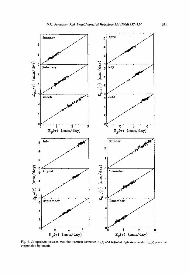
where 0p is the dependent variable Epa , f l , g l , f2 or g2- The coefficients h0 to h 7 a r e shown in Table 5 and their corresponding Student t-ratios and adjusted R E values are shown in Table 6. Fig. 4 compares Ep( ' r ) and Ep,r(7-) month by month, illustrating that Ep,r(7-) provides a good estimate of Ep(-r) a c r o s s all sites.

5.1. Comparison with other studies

It is useful to examine how well the regression model Ep.r(r) compares with another temperature-based models of potential evaporation. Linacre (1977) presented a temperature-based model for estimating potential evaporation Ep,L(r). As with Linacre's Et,L(r) model, Ep,L(r) requires mean monthly temperature and location latitude and elevation.

5.2. Goodness-of-fit comparison

As with the evaluation between Et(7") with Et , r ( r ) , Et,H(7" ) and Et,L(r), we employ the monthly bias, BIAS, and monthly root mean square error, r.m.s.e., described by Eq. (9) and Eq. (10), respectively, to compare the modified Penman equation Ep(r) against the regression method (Ep,r(r)) and the Linacre method (Ep,L(r)) estimates.


0 e~

~ 2

~ 0 r~

I Janu~y Jl

March

I L 0

0 1 2

Ep(7) ( m m / d a y )

6 April

. . . . I

0 4 June . . . . . . . .

0 2 4 6

Ep('r) ( r a m / d a y )

6 July ~ October

2

~ . . . . . ~ o

2

i~, ~ o

o o ~ - - - - ~ 0 2 4 6 0 1 2 3

Ep(7) (ram/day) Sp(7) (ram/day)

Fig. 4. Comparison between modified Penman estimated EpQ') and regional regression model Et.p(-r ) potential evaporation by month.


Table 7 A comparison of monthly BIAS and r.m.s.e, for the two estimators Ep,r(r) and Ep,L(r)

r Month BIAS[w]

w = Ep,r(r ) w = Ev,L(r ) (mm day -1) (mm day -1)

1 January 0.00 -0.63 2 February 0.04 -0.84 3 March 0.00 -0.68 4 April -0.06 -0.10 5 May 0.10 0.58 6 June 0.02 1.39 7 July -0.04 2.28 8 August 0.02 2.69 9 September 0.05 2.48 10 October -0.02 1.72 11 November -0.01 0.81 12 December 0.02 -0.21

r Month r.m.s.e.[w]

W = Ep,r('r ) w = Ep,L(7") (mm day -1) (mm day -1)

1 January 0.08 0.67 2 February 0.08 0.88 3 March 0.08 0.77 4 April 0.12 0.41 5 May 0.16 0.70 6 June 0.16 1.42 7 July 0.17 2.28 8 August 0.13 2.68 9 September 0.12 2.47 10 October 0.10 1.72 11 November 0.08 0.84 12 December 0.08 0.36

Similar to our previous goodness-of-f i t evaluat ion, 33 separate sets of the five regional

regression equat ions for Epa, f l , f2, gl and g2 were developed to more fairly est imate the BIAS and r.m.s.e, be tween Ep(r) and Ep,r(r). Each regression est imator in this evaluat ion for a part icular site, Ep,r(7), is based on temperature, longi tude and elevat ion data from the 33 other sites.

Table 7 documents the BIAS and r.m.s.e, for each method--Ep,r ( r ) and Et,L(Z). Clearly, the regression model Ep,r(7 ) provides the lowest overall BIAS and r.m.s.e. Practically speaking, even the largest single monthly BIAS of 0.09 m m day -1 would be difficult to measure.

6. Summary and conclusions

This study developed regional statistical models of est imated month ly average reference crop evapotranspirat ion, Et(r), where z = 1,12, and est imated month ly evaporation,


Ep(~') based upon the Penman-Monte i th method. Et(7") is determined for a reference grass vegetation. Estimates for Et(7") and Ep0- ) derived from the Penman-Monte i th equation require air temperature, relative humidity or dewpoint temperature, windspeed and cloud cover, data which are generally available only at sparsely located N O A A First Order weather observatories. The regional estimators presented here, Et,r(7") and Ep,r(7"), require only monthly average air temperature, and the si te 's longitude and elevation. The models are shown to provide excellent estimates of Et(7 ) and Ep(r) for all locations in the northeastern U S A ranging from eastern Ohio through central Virginia to northern Maine, including mountain and coastal areas. Ep,r(r) is shown to be a significant improvement over the Linacre (1977) temperature method to estimate Ep(r). Et,r(7") is shown be an improvement over both the Linacre (1977) and Hargreaves and Samani (1985) temperature methods to estimate Et(7" ) in the northeastern USA.

Acknowledgements

This work was funded in part by the Massachusetts Department of Environmental Protection, Office of Watershed Management and the Division of Water Supply, and in part by the US Environmental Protection Agency Assistance Agreement CR820301 to the Tufts University Center for Environmental Management. The authors express their appre- ciation for the very helpful review comments by Dr. Dara Entekhabi and three anonymous reviewers, who all contributed to substantially improving the original manuscript.

References

Bloomfield, P., 1976. Fourier Analysis of Time Series: An Introduction. Wiley, New York. Bras, R.L., 1991. Hydrology; an Introduction to Hydrologic Science. Addison-Wesley, Reading, MA. Brest, C.L., 1987. Seasonal albedo of an urban/rural landscape from satellite observations. J. Climate Appl.

Meteorol., 26(9): 1169-1187. Brutsaert, W., 1984. Evaporation into the Atmosphere: Theory, History and Applications. D. Reidel, Boston, MA. Eagleson, P.S., 1970. Dynamic Hydrology. McGraw-Hill, New York. Fennessey, N.M., 1994. A hydro-climatological model of daily streamflow for the northeast United States. Ph.D.

Dissertation, Tufts University, Medford, MA. Fennessey, N.M. and Kirshen, P.H., 1994. Evaporation and evapotranspiration under climate change in New

England. ASCE J. Water Resour. Plann. Manage., 120(1): 48-69. Hargreaves, G.H., 1994. Defining and using reference evapotranspiration. ASCE J. Irrig. Drainage Eng., 120(6):

1132-1139. Hargreaves, G.H. and Samani, Z.A., 1985. Reference crop evapotranspiration. Appl. Eng. Agric., 1(2): 96-99. Hirsch, R.M., Helsel, D.R., Cohn, T.A. and Gilroy, E.J., 1993. Statistical analysis of hydrologic data. In: D.R.

Maidment (Editor), Handbook of Hydrology. McGraw-Hill, New York. Jensen, M.E., Burman, R.D. and Allen, R.G., 1990. Evapotranspiration and irrigation water requirements. ASCE

Manual 70. ASCE, New York, 332 pp. Linacre, E.T., 1977. A simple formula for estimating evaporation rates in various climates, using temperature data

alone. Agric. Meteorol., 18: 409-424. Monteith, J.L., 1965. Evaporation and the environment. The state and movement of water in living organisms.

Symp. Soc. Exp. Biol., XIX. Penman, H.L., 1948. Natural evaporation from open water, bare soil and grass. Proc. R. Soc. London, Ser. A, 193:

120-148.


Shuttleworth, W.J., 1993. Evaporation. In: D.R. Maidment (Editor), Handbook of Hydrology. McGraw-Hill, New York.

Stedinger, J.R., Vogel, R.M. and Foufoula-Georgiou, E., 1993, Frequency analysis of extreme events. In: D.R. Maidment (Editor), Handbook of Hydrology. McGraw-Hill, New York.

Thornthwaite, C.W., 1948. An approach toward a rational classification of climate. Am. Geogr. Rev., 38: 55-94. Van Bavel, C.H.M., 1966. Potential evaporation: the combination concept and its experimental verification.

Water Resour. Res., 2(3): 455-467.

Documents

Regional models of potential evaporation and reference ...engineering.tufts.edu/cee/people/vogel/documents/regional... · Regional models of potential evaporation and reference evapotranspiration