Regional Disparities in the Spatial Correlation of State Income Growth

8/14/2019 Regional Disparities in the Spatial Correlation of State Income Growth

http://slidepdf.com/reader/full/regional-disparities-in-the-spatial-correlation-of-state-income-growth 1/19

Ann Reg Sci (2007) 41:601–618DOI 10.1007/s00168-007-0114-x

O R I G I N A L PA P E R

Regional disparities in the spatial correlation of state

income growth, 1977–2002

Thomas A. Garrett · Gary A. Wagner ·

David C. Wheelock

Received: 16 December 2005 / Accepted: 19 December 2006 / Published online: 9 February 2007© Springer-Verlag 2007

Abstract This paper presents new evidence of spatial correlation in USAstate income growth. We extend the basic spatial econometric model used inthe growth literature by allowing spatial correlation in state income growth tovary across geographic regions. We find positive spatial correlation in incomegrowth rates across neighboring states, but that the strength of this spatial cor-relation varies considerably by region. Spatial correlation in income growth is

highest for states located in the Northeast and the South. Our findings havepolicy implications both at the state and national level, and also suggest thatgrowth models may benefit from incorporating more complex forms of spatialcorrelation.

JEL Classification G28 · C23 · R10

The views expressed here are those of the authors and not those of the Federal Reserve Bank of St Louis or the Federal Reserve System.

T. A. Garrett · D. C. WheelockFederal Reserve Bank of St Louis Research Division, PO Box 442,St Louis, MO 63166-0442, USAe-mail: [email protected]

D. C. Wheelocke-mail: [email protected]



602 T. A. Garrett et al.

1 Introduction

In recent years, it has become common to use spatial econometric techniques toinvestigate the role of location as a determinant of economic growth (seeAbreu

et al. 2005 for a survey). From the estimation of a variety of cross-country andsub-national models, the literature has generally concluded that a country orregion’s growth can be substantially dependent on the growth (or lack thereof)of other countries or regions.

Although the models of spatial correlation appearing in the literature do vary,they all share a common characteristic in that they restrict potential spatial cor-relations between countries or regions to be the same across all geographicdivisions in the sample. Evidence of regional differences in economic perfor-mance during national business cycles and in response to economic integration

both in the European Union and United States suggests, however, that theinfluence of spatial correlations among neighbors could vary across regions.1 Inthis paper we extend the typical spatial econometric model of growth to allowfor regional variation in spatial correlations. We estimate the model using dataon USA states, for which control variables have been extensively researched(see Crain and Lee 1999) and where measurement problems are less thornythan with a cross-country study.

Consistent with the broader literature, we find evidence of positive spatialcorrelation in state-level income growth across the USA as a whole. That is,

when spatial correlation is assumed to affect all states equally, we find thata given state’s income growth is directly related to the income growth of itsneighbors. However, when we allow for regional differences in the impact of spatial correlation in state income growth, we find large and statistically sig-nificant differences across regions in the effects of spatial correlation. Sincethe regional-specific spatial models also “fit-the-data” better than the standardmodels with common spatial effects, our results suggest that more complexforms of spatial correlation may be at work in growth dynamics.

2 Literature review

Although the connection between location and growth is deep-rooted,DeLongand Summers (1991) were the first to discuss the possibility that spatial patternsmay exist in standard cross-country growth regressions. They observed thatsince omitted variables in neighboring countries are likely to take on similarvalues, citing the similarities between Belgium and the Netherlands as an illus-tration, the residuals from a “standard” growth regression could be correlatedacross countries. Although DeLong and Summers (1991) found no evidence of

spatially correlated residuals in their data, their recognition of the potential forspatial correlation prompted further examination. Over the past several years,






permits growth in a state’s income to depend on the state’s initial income andthe initial income of neighboring states (those sharing a common border in theframework of Rey and Montouri 1999), while the spatial error model allowscorrelation in model errors across states. In both spatial econometric specifica-

tions, as well as a baseline model that excludes spatial effects,Rey and Montouri(1999) find evidence to support unconditional β-convergence. The spatial lagand spatial error coefficients are found to be significant at the one percent level,with the results of specification tests indicating the spatial error model may bemore appropriate. A number of subsequent studies, with a largely Europeanfocus, have applied the basic spatial growth framework of Rey and Montouri(1999) and found similar results using a variety of different time periods andgeographic focus.2

The focus of our paper differs from previous work in two important ways.

First, we estimate a short-run model of growth for USA states, as opposed to along-run (i.e., convergence) model. This allows us to not only avoid the potentialfor structural differences that may arise in a cross-country framework, but alsoavoid the criticisms of convergence models in general (Quah 1993, 1996). Inaddition, since convergence models are tested by regressing income growth oninitial income, and possibly other control variables, it would seem to be the casethat any spatial growth effects uncovered in these models are a result of long-rundynamics. However, with regard to USA states, there is considerable evidenceto suggest that short-run growth dynamics may also be spatially related. For

example, Carlino and Sill (2001) find evidence of regional linkages in the trendand cyclical components of real per capita personal income for Bureau of Eco-nomic Analysis (BEA) regions within the United States. Applying a vectorerror correction model to quarterly data from 1956 to 1995, Carlino and Sill(2001) find that regional income growth is cointegrated across BEA regions,which indicates that the regions share a common long-run growth path. Thelinkages are not as strong with regard to the cyclical component, however. Thecyclical component of the Far West region is “out-of-synch” with the cyclicalcomponents of the nation and other regions (the Far West has a simple cor-

relation of 0.36 with the nation, compared to an average of 0.97 for the otherregions). From the perspective of growth regressions, these findings suggest thatwhile sub-regions of the USA appear to converge, there is reason to suspectthe presence of spatial correlation in transitory deviations from trend. Thus, atransitory shock that affects growth in a given state may affect growth in otherstates, and the strength of the spillovers may differ across sub-regions of theUnited States.

A second difference between our study and prior work is that we allow spa-tial correlation in state income growth to vary across regions of the UnitedStates. Carlino and Sill’s (2001) finding of regional cyclical components in stateincome growth suggests regional heterogeneity in the influence of spatial effects.An apparent difference in the influence of changes in monetary policy across



Regional disparities in the spatial correlation of state income growth 605

regions (Carlino and DeFina 1999) is one possible reason for this heterogeneity.Prior research has found evidence of regional heterogeneity in agriculture andstate bank regulatory policies (e.g., Garrett et al. 2005) but regional differencesin the spatial correlation of state economic growth has not been explored. The

advantage of allowing any spatial correlation in state income growth to varyacross regions is that we are able to formally test for regional disparities in stateincome growth. The possibility of regional differences in spillovers in stateincome growth has implications for both state and national policies that effecteconomic growth.

3 Data and empirical specification

We use the basic model of spatial correlation developed byCliff and Ord (1981)and Anselin (1988) to investigate the determinants of state-level annual incomegrowth in the 48 contiguous states over the period 1977–2002.3 The general spa-tial model allows for potential spatial correlation in both the dependent variableand error term. It does not induce cross-sectional correlation if none is pres-ent; it simply provides an established and flexible framework for relaxing theassumption of cross-sectional correlation with regard to a model’s dependentvariable and/or error term. As Anselin (1988) notes, unlike time-series corre-lation that is 1D, spatial correlation in cross-sectional models is multi-dimen-sional in that it depends upon all contiguous or influential units of observations

(in this case states). Formally, the general first-order spatial model may beexpressed as:

y = ρW y + X β + ε (1a)

ε = λW ε + ν = ( I − λW )−1ν (1b)

where y is the (TN × 1) vector of growth rates in real per capita state personalincome and X is a (TN × K) matrix of regressors. The spatial lag componentis given by ρW y, where W denotes the exogenous (TN × TN) block diagonalmatrix composed of the (N × N) spatial weights matricesw along T block diag-onal elements. The scalar ρ is the spatial lag coefficient that must be estimated.Positive spatial correlation exists if ρ > 0, negative spatial correlation if ρ < 0,and no spatial correlation if ρ = 0.4 The spatial error component of the modelis given by ε = λW ε + ν, where is a (TN × 1) vector of error terms, W isthe (TN × TN) matrix previously described, ν is a (TN × 1) white noise error

3 Because we use Crain and Lee’s (1999) measure of industry diversity in our regressions, whichis constructed using Gross State Product (GSP) data, the starting date of our sample is limited to1977 because this is the first year that GSP data are available.4 Unlike the standard first-order autoregressive model in time series, the spatial correlation coeffi-




component, and λ is the spatial error coefficient that must be estimated. Theerrors are positively correlated if λ > 0, negatively correlated if λ < 0, andspatially uncorrelated correlated if λ = 0. Note that if no spatial correlation of any form exists, then ρ = λ = 0 and the general spatial model reduces to the

standard regression model.Since the spatial lag term in Eq. 1a is correlated with the error term and the

spatial error component is also non-spherical, ordinary least squares (OLS)estimation of Eqs. 1a and b will result in biased, inconsistent, and ineffi-cient parameter estimates (Anselin 1988). Assuming the random componentof the spatial error (ν) is homoskedastic and jointly normally distributed,Eqs. 1a and b can be estimated by maximum likelihood. Anselin (1988) de-rives the log-likelihood function for the general spatial model, which can beexpressed as:

= −

NT

2

ln(π ) −

1

2

ln

σ 2ν

+ ln | I − ρW |

+ ln | I − λW | −

ψ ϕ ϕ ψ

2σ 2ν

, (2)

where ψ = y − ρW y − X β, ϕ = I − λW , and I is a TN × TN identity matrix.The cross-sectional spatial weights matrix (w) formalizes the potential cor-

relation among states for which many alternative representations have beenused in the literature. We consider two specifications of w in our empiricalanalyses. First, a common weights matrix in the growth literature (and spatialeconometrics literature in general) is the binary contiguity matrix (Cliff andOrd 1981, Anselin 1988, Case 1992). In this representation, the individual ele-ments of w, denoted ωij, are set equal to unity if states i and j (i = j ) share acommon border, and to zero otherwise. The limitations of this specification arethat all neighboring states are assumed to have equal influence and any spatialcorrelations beyond common-border neighbors are ignored.5

In addition to a common-border weights matrix, we also consider distance asan alternative spatial weighting scheme. Distance-based weighting has beenused in several studies, such as Dubin (1988), Garrett and Marsh (2002),Hernandez (2003), and Garrett et al. (2005), but has not been widely exploitedin the growth literature. The most established distance-based weighting scheme,and the one we implement in this paper, is an inverse distance format whereωij = 1/dij , and dij is the distance between states i and j . In addition, ωij = 0for i = j . Thus, as the distance between states i and j increases (decreases),ωij decreases (increases), which gives less (more) spatial weight to the state

pair when i = j . Since there is no consensus in the literature on how dis-tance should be measured, we follow Hernandez (2003) and measure distance




as the difference between state population centers.6 This weighting scheme isvery intuitive and extends any potential spatial correlation beyond common-border neighbors since all states are spatially related, but nearer states (mea-sured by the proximity of their population centers) have a greater potential

influence.The basic spatial model detailed above assumes that the influence of spatial

correlation is the same for all states. That is, the functional form given by Eqs.1aand b does not permit regional differences in either the spatial lag or spatialerror. We modify Eqs. 1a and b to allow for different spatial correlation coeffi-cients in different regions of the United States. We use both region and divisionclassifications by the USA Bureau of the Census. There are nine Census Bureaudivisions in the contiguous 48 states and four regions. The spatial model withregional spatial correlation coefficients may be written as:

y =

Rk=1

ρkW k y + X β + ε (3a)

ε =

Rk=1

λkW kε + ν =

I −

Rk=1

λkW k

−1

ν, (3b)

where R denotes the total number of regions, and ρk and λk denote the spatial

lag and spatial error lag coefficients, respectively, for regionk. W k remains the(TN × TN) block diagonal matrix having (N× N) spatial weights matrices wk

along T block diagonal elements. Each matrix wk is constructed by pre-multi-plying by a dummy variable that equals unity if state i is located in region k,and zero otherwise7. This provides a different interpretation of wk dependingupon whether wk is a contiguity weight matrix or a distance weight matrix. Inthe case of a contiguity matrix, we allow growth in state i located in region k tobe affected by the income growth of all states j that border state i, regardless of whether state j is in the same region as state i. With the distance weights matrix,

the elements of each matrix wk capture spatial correlation between each statein region k and the remaining 47 states. Thus, for each state i in region k, rowi of distance matrix wk contains some measure of distance between state i andall remaining 47 states. If state i is not in region k, then row i of distance matrixwk contains all zeros.

The matrix ( X ) includes variables that Crain and Lee (1999) have shown tosignificantly affect state income growth. They use an Extreme-Bounds Anal-ysis (EBA) to test the robustness of 29 different control variables in growth

6 The distance was computed using the geographic coordinates for the population centroids com-puted by the Bureau of the Census for the year 2000. Population centroids did not differ significantlyi l d d




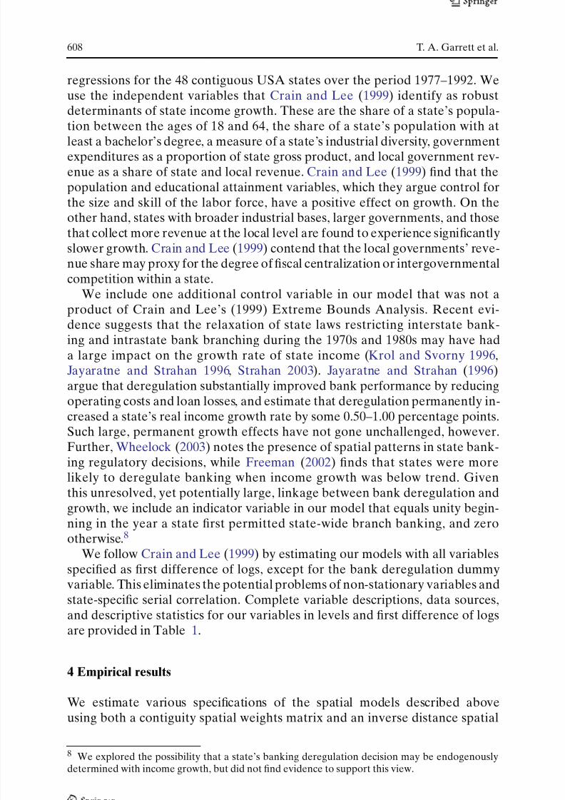
regressions for the 48 contiguous USA states over the period 1977–1992. Weuse the independent variables that Crain and Lee (1999) identify as robustdeterminants of state income growth. These are the share of a state’s popula-tion between the ages of 18 and 64, the share of a state’s population with at

least a bachelor’s degree, a measure of a state’s industrial diversity, governmentexpenditures as a proportion of state gross product, and local government rev-enue as a share of state and local revenue. Crain and Lee (1999) find that thepopulation and educational attainment variables, which they argue control forthe size and skill of the labor force, have a positive effect on growth. On theother hand, states with broader industrial bases, larger governments, and thosethat collect more revenue at the local level are found to experience significantlyslower growth. Crain and Lee (1999) contend that the local governments’ reve-nue share may proxy for the degree of fiscal centralization or intergovernmental

competition within a state.We include one additional control variable in our model that was not a

product of Crain and Lee’s (1999) Extreme Bounds Analysis. Recent evi-dence suggests that the relaxation of state laws restricting interstate bank-ing and intrastate bank branching during the 1970s and 1980s may have hada large impact on the growth rate of state income (Krol and Svorny 1996,Jayaratne and Strahan 1996, Strahan 2003). Jayaratne and Strahan (1996)argue that deregulation substantially improved bank performance by reducingoperating costs and loan losses, and estimate that deregulation permanently in-

creased a state’s real income growth rate by some 0.50–1.00 percentage points.Such large, permanent growth effects have not gone unchallenged, however.Further, Wheelock (2003) notes the presence of spatial patterns in state bank-ing regulatory decisions, while Freeman (2002) finds that states were morelikely to deregulate banking when income growth was below trend. Giventhis unresolved, yet potentially large, linkage between bank deregulation andgrowth, we include an indicator variable in our model that equals unity begin-ning in the year a state first permitted state-wide branch banking, and zerootherwise.8

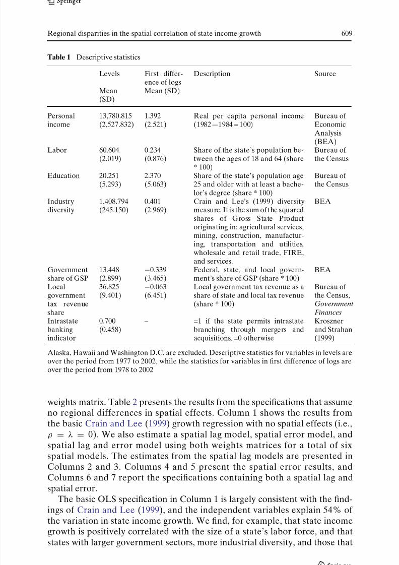
We follow Crain and Lee (1999) by estimating our models with all variablesspecified as first difference of logs, except for the bank deregulation dummyvariable. This eliminates the potential problems of non-stationary variables andstate-specific serial correlation. Complete variable descriptions, data sources,and descriptive statistics for our variables in levels and first difference of logsare provided in Table 1.

4 Empirical results

We estimate various specifications of the spatial models described aboveusing both a contiguity spatial weights matrix and an inverse distance spatial




Table 1 Descriptive statistics

Levels First differ-ence of logs

Description Source

Mean

(SD)

Mean (SD)

Personalincome

13,780.815(2,527.832)

1.392(2.521)

Real per capita personal income(1982—1984 = 100)

Bureau of EconomicAnalysis(BEA)

Labor 60.604(2.019)

0.234(0.876)

Share of the state’s population be-tween the ages of 18 and 64 (share* 100)

Bureau of the Census

Education 20.251(5.293)

2.370(5.063)

Share of the state’s population age25 and older with at least a bache-lor’s degree (share * 100)

Bureau of the Census

Industrydiversity

1,408.794(245.150)

0.401(2.969)

Crain and Lee’s (1999) diversitymeasure. It is the sum of the squaredshares of Gross State Productoriginating in: agricultural services,mining, construction, manufactur-ing, transportation and utilities,wholesale and retail trade, FIRE,and services.

BEA

Governmentshare of GSP

13.448(2.899)

−0.339(3.465)

Federal, state, and local govern-ment’s share of GSP (share * 100)

BEA

Local

governmenttax revenueshare

36.825

(9.401)

−0.063

(6.451)

Local government tax revenue as a

share of state and local tax revenue(share * 100)

Bureau of

the Census,Government

Finances

Intrastatebankingindicator

0.700(0.458)

– =1 if the state permits intrastatebranching through mergers andacquisitions, =0 otherwise

Krosznerand Strahan(1999)

Alaska, Hawaii and Washington D.C. are excluded. Descriptive statistics for variables in levels areover the period from 1977 to 2002, while the statistics for variables in first difference of logs areover the period from 1978 to 2002

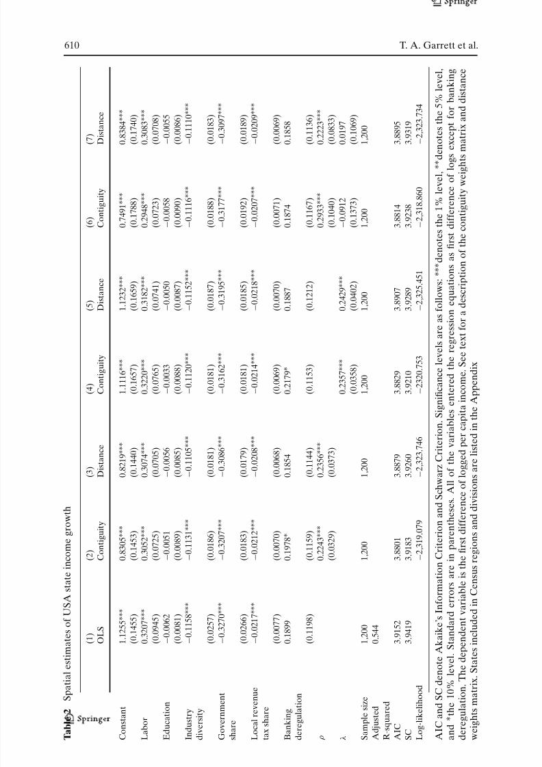
weights matrix. Table 2 presents the results from the specifications that assumeno regional differences in spatial effects. Column 1 shows the results fromthe basic Crain and Lee (1999) growth regression with no spatial effects (i.e.,ρ = λ = 0). We also estimate a spatial lag model, spatial error model, andspatial lag and error model using both weights matrices for a total of sixspatial models. The estimates from the spatial lag models are presented inColumns 2 and 3. Columns 4 and 5 present the spatial error results, andColumns 6 and 7 report the specifications containing both a spatial lag andspatial error.

The basic OLS specification in Column 1 is largely consistent with the find-ings of Crain and Lee (1999), and the independent variables explain 54% of




S p a t i a l e s t i m a t e s o f U S A s t a t e i n c o m e g r o w t h

( 1 )

( 2 )

( 3 )

( 4 )

( 5 )

( 6 )

( 7 )

O L S

C o n t i g u i t y

D i s t a n c e

C o n t i g u i t y

D i s t a n c e

C o n t i g u i t y

D i s

t a n c e

1 . 1 2 5 5 ∗ ∗ ∗

0 . 8 3 0 5 ∗ ∗ ∗

0 . 8 2 1 9 ∗ ∗ ∗

1 . 1 1 1 6 ∗ ∗ ∗

1 . 1 2 3 2 ∗ ∗ ∗

0 . 7 4 9 1 ∗ ∗ ∗

0 . 8 3 8 4 ∗ ∗ ∗

( 0 . 1

4 5 5 )

( 0 . 1

4 5 3

)

( 0 . 1

4 4 0 )

( 0 . 1

6 5 7 )

( 0 . 1

6 5 9 )

( 0 . 1

7 8 8 )

( 0 . 1

7 4 0 )

0 . 3 2 0 7 ∗ ∗ ∗

0 . 3 0 5 2 ∗ ∗ ∗

0 . 3 0 7 4 ∗ ∗ ∗

0 . 3 2 2 0 ∗ ∗ ∗

0 . 3 1 8 2 ∗ ∗ ∗

0 . 2 9 4 8 ∗ ∗ ∗

0 . 3 0 8 3 ∗ ∗ ∗

( 0 . 0

9 4 5 )

( 0 . 0

7 2 5

)

( 0 . 0

7 0 5 )

( 0 . 0

7 6 5 )

( 0 . 0

7 4 1 )

( 0 . 0

7 2 3 )

( 0 . 0

7 0 8 )

− 0 . 0 0 6 2

− 0 . 0 0 5

1

− 0 . 0 0 5 6

− 0 . 0 0 3 3

− 0 . 0 0 5 0

− 0 . 0 0 5 8

− 0 . 0

0 5 5

( 0 . 0

0 8 1 )

( 0 . 0

0 8 9

)

( 0 . 0

0 8 5 )

( 0 . 0

0 8 8 )

( 0 . 0

0 8 7 )

( 0 . 0

0 9 0 )

( 0 . 0

0 8 6 )

− 0 . 1 1 5 8 ∗ ∗ ∗

− 0 . 1 1 3

1 ∗ ∗ ∗

− 0 . 1 1 0 5 ∗ ∗ ∗

− 0 . 1 1 2 0 ∗ ∗ ∗

− 0 . 1 1 5 2 ∗ ∗ ∗

− 0 . 1 1 1 6 ∗ ∗ ∗

− 0 . 1

1 1 0 ∗ ∗ ∗

( 0 . 0

2 5 7 )

( 0 . 0

1 8 6

)

( 0 . 0

1 8 1 )

( 0 . 0

1 8 1 )

( 0 . 0

1 8 7 )

( 0 . 0

1 8 8 )

( 0 . 0

1 8 3 )

n t

− 0 . 3 2 7 0 ∗ ∗ ∗

− 0 . 3 2 0

7 ∗ ∗ ∗

− 0 . 3 0 8 6 ∗ ∗ ∗

− 0 . 3 1 6 2 ∗ ∗ ∗

− 0 . 3 1 9 5 ∗ ∗ ∗

− 0 . 3 1 7 7 ∗ ∗ ∗

− 0 . 3

0 9 7 ∗ ∗ ∗

( 0 . 0

2 6 6 )

( 0 . 0

1 8 3

)

( 0 . 0

1 7 9 )

( 0 . 0

1 8 1 )

( 0 . 0

1 8 5 )

( 0 . 0

1 9 2 )

( 0 . 0

1 8 9 )

n u e

− 0 . 0 2 1 7 ∗ ∗ ∗

− 0 . 0 2 1

2 ∗ ∗ ∗

− 0 . 0 2 0 8 ∗ ∗ ∗

− 0 . 0 2 1 4 ∗ ∗ ∗

− 0 . 0 2 1 8 ∗ ∗ ∗

− 0 . 0 2 0 7 ∗ ∗ ∗

− 0 . 0

2 0 9 ∗ ∗ ∗

( 0 . 0

0 7 7 )

( 0 . 0

0 7 0

)

( 0 . 0

0 6 8 )

( 0 . 0

0 6 9 )

( 0 . 0

0 7 0 )

( 0 . 0

0 7 1 )

( 0 . 0

0 6 9 )

0 . 1 8 9 9

0 . 1 9 7 8 ∗

0 . 1 8 5 4

0 . 2 1 7 9 ∗

0 . 1 8 8 7

0 . 1 8 7 4

0 . 1 8 5 8

n

( 0 . 1

1 9 8 )

( 0 . 1

1 5 9

)

( 0 . 1

1 4 4 )

( 0 . 1

1 5 3 )

( 0 . 1

2 1 2 )

( 0 . 1

1 6 7 )

( 0 . 1

1 3 6 )

0 . 2 2 4 3 ∗ ∗ ∗

0 . 2 3 5 6 ∗ ∗ ∗

0 . 2 9 3 3 ∗ ∗ ∗

0 . 2 2 2 3 ∗ ∗ ∗

( 0 . 0

3 2 9

)

( 0 . 0

3 7 3 )

( 0 . 1

0 4 0 )

( 0 . 0

8 3 3 )

0 . 2 3 5 7 ∗ ∗ ∗

0 . 2 4 2 9 ∗ ∗ ∗

− 0 . 0 9 1 2

0 . 0 1 9 7

( 0 . 0

3 5 8 )

( 0 . 0

4 0 2 )

( 0 . 1

3 7 3 )

( 0 . 1

0 6 9 )

1 , 2 0 0

1 , 2 0 0

1 , 2 0 0

1 , 2 0 0

1 , 2 0 0

1 , 2 0 0

1 , 2 0 0

0 . 5 4 4

3 . 9 1 5 2

3 . 8 8 0 1

3 . 8 8 7 9

3 . 8 8 2 9

3 . 8 9 0 7

3 . 8 8 1 4

3 . 8 8 9 5

3 . 9 4 1 9

3 . 9 1 8 3

3 . 9 2 6 0

3 . 9 2 1 0

3 . 9 2 8 9

3 . 9 2 3 8

3 . 9 3 1 9

o o d

− 2 , 3 1 9

. 0 7 9

− 2 , 3 2 3 . 7 4 6

− 2 3 2 0 . 7

5 3

− 2 , 3 2 5 . 4 5 1

− 2 , 3 1 8 . 8 6 0

− 2 , 3

2 3 . 7

3 4

S C d e n o t e A k a i k e ’ s I n f o r m a t i o n C r i t e r

i o n a n d S c h w a r z C r i t e r i o n .

S i g n

i fi c a n c e l e v e l s a r e a s f o l l o w s : ∗ ∗ ∗ d e n o t e s t h e 1 % l e v e l , ∗ ∗ d e n o t e

s t h e 5 % l e v e l ,

1 0 % l e

v e l . S t a n d a r d e r r o r s a r e i n p a r e n t h e s e s .

A l l o f t h e v a r i a b l e s e n t e r e d t h e r e g r e s s i o n e q u a t i o n s a s fi r s t d i f f e r e n c e o f l o g s e x c e

p t f o r b a n k i n g

o n . T h e d e p e n d e n t v a r i a b l e i s t h e fi r s t

d i f f e r e n c e o f l o g g e d p e r c a p i t a i n c o m e . S e e t e x t f o r a d e s c r i p t i o n o f t h e c o n t i g u i t y w e i g h t s m a t r i x a n d d i s t a n c e

a t r i x . S

t a t e s i n c l u d e d i n C e n s u s r e g i o n s a n d d i v i s i o n s a r e l i s t e d i n t h e A

p p e n d i x




collect more revenue at the local rather than state level experience significantlyslower income growth. We also find that growth is uncorrelated with educa-tional attainment.9 In addition, we find little evidence that bank deregulationresults in significantly higher growth, which is consistent with Freeman (2002,

2005).Consistent with the growth and convergence literature, the results reported

in Columns 2–5 of Table 2 reveal strong evidence of spatial correlation. Fur-thermore, regardless which weights matrix we use, the coefficients on ρ and λ

are quite similar in magnitude and statistically significant at the 1% level. Theestimated spatial lag coefficients are all positive, indicating that a state’s incomegrowth is directly affected by the income growth of neighboring states. The esti-mates of ρ from columns 2 to 3 indicate that a one percentage point increase inthe average income growth of “neighboring” states generates a 0.23% increase

in state is income growth rate, regardless whether “neighboring” states includeonly the states that share a border with state i or all states, with nearer stateshaving more influence.

In contrast to ρ, the interpretation of λ is analogous to an estimate of first-order serial correlation in a time-series regression. The positive and significantestimates for λ that appear in Columns 4 and 5 indicate that there is evidenceof significant positive residual correlation across space, which could be due tospatial heterogeneity or omitted variables. However, the Akaike InformationCriterion (AIC), Schwarz Criterion (SC) and the log-likelihood statistics all

reveal that the spatial lag models presented in Columns 2 and 3 provide abetter fit than the spatial error models.The results from the models that include both the spatial lag and error term

(Columns 6 and 7) reveal that only the spatial lag coefficients are significantlydifferent from zero and have magnitudes very similar to those presented inColumns 2 and 3. This suggests that the significant spatial error coefficientsin Columns 4 and 5 were likely capturing omitted spatial correlation in stateincome growth. The findings presented in Table 2 suggest that spatial correla-tion in state-level income growth may be best modeled using a spatial lag. This

is supported by the AIC and SC, which are directly comparable across modelsand weigh the explanatory power of a model (based on the maximized valueof the log-likelihood function) against parsimony. Based on the AIC and SC,all of the spatial models are preferred to the OLS specification, but the spatiallag model that utilizes the contiguity weights matrix provides the best fit of the data.

Finally, it is also interesting to note that the inclusion of the spatial effectshas little impact on the estimated parameters for the control variables. Wefind the banking deregulation indicator to be significant at the 10% level inColumns 2 and 4 in Table 2, but the magnitude and significance of the remain-ing independent variables are largely unchanged.






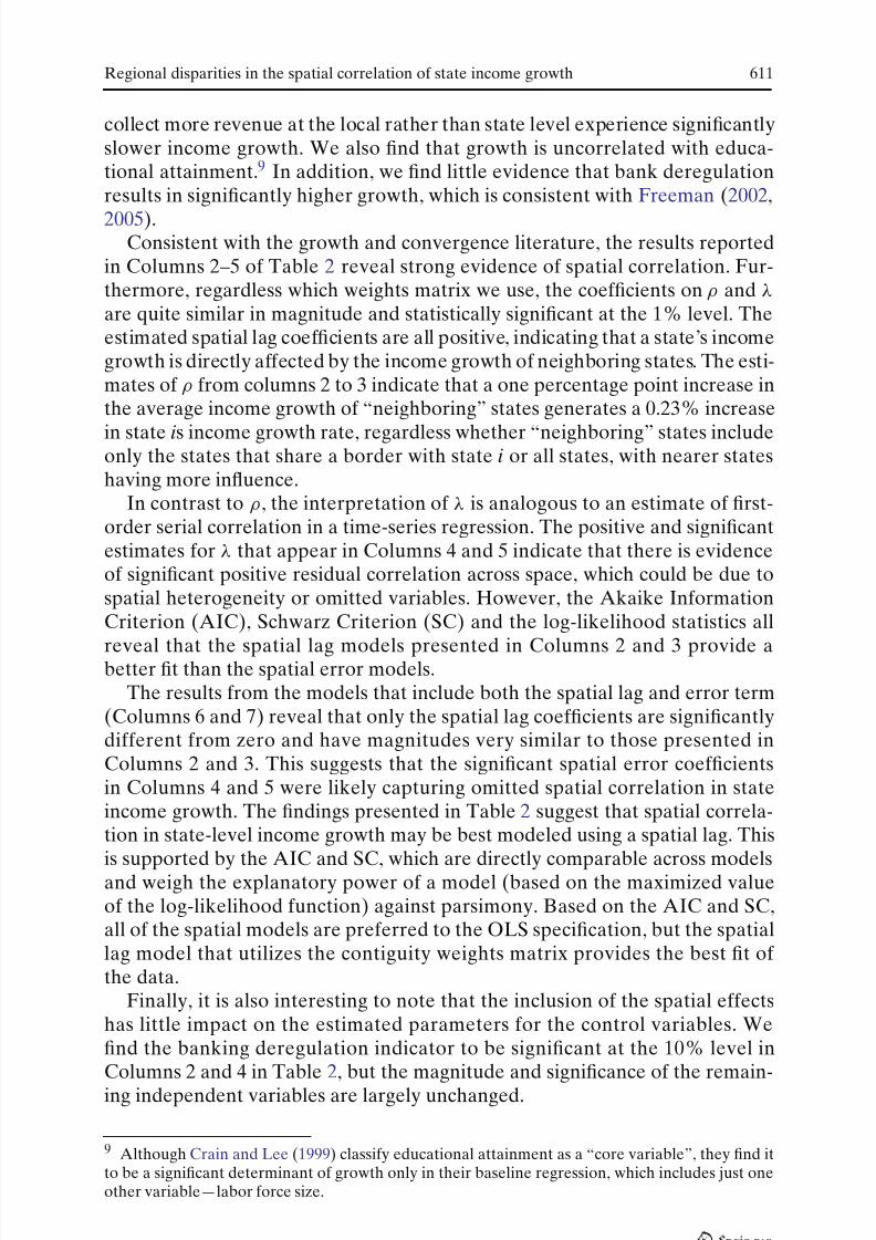
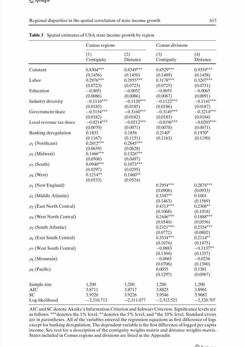
Table 3 Spatial estimates of USA state income growth by region

Census regions Census divisions

(1) (2) (3) (4)

Contiguity Distance Contiguity Distance

Constant 0.8304∗∗∗ 0.8349∗∗∗ 0.8529∗∗∗ 0.9359∗∗∗

(0.1456) (0.1450) (0.1489) (0.1458)Labor 0.2976∗∗∗ 0.2955∗∗∗ 0.3178∗∗∗ 0.3207∗∗∗

(0.0723) (0.0723) (0.0725) (0.0731)Education −0.0051 −0.0052 −0.0059 −0.0065

(0.0086) (0.0086) (0.0087) (0.0091)Industry diversity −0.1116∗∗∗ −0.1120∗∗∗ −0.1122∗∗∗ −0.1141∗∗∗

(0.0185) (0.0185) (0.0186) (0.0187)Government share −0.3154∗∗∗ −0.3160∗∗∗ −0.3149∗∗∗ −0.3214∗∗∗

(0.0182) (0.0182) (0.0183) (0.0184)

Local revenue tax share −0.0214∗∗∗ −0.0212∗∗∗ −0.0196∗∗∗ −0.0203∗∗∗

(0.0070) (0.0071) (0.0070) (0.0071)Banking deregulation 0.1833 0.1856 0.2140∗ 0.1970∗

(0.1167) (0.1151) (0.1163) (0.1190)ρ1 (Northeast) 0.2812∗∗∗ 0.2845∗∗∗

(0.0639) (0.0628)ρ2 (Midwest) 0.1466∗∗∗ 0.1326∗∗∗

(0.0508) (0.0497)ρ3 (South) 0.0940∗∗∗ 0.1073∗∗∗

(0.0297) (0.0295)ρ4 (West) 0.1214∗∗ 0.1060∗∗

(0.0533) (0.0524)ρ1 (New England) 0.2954∗∗∗ 0.2874∗∗∗

(0.0908) (0.0933)ρ2 (Middle Atlantic) 0.3347∗∗ 0.1001

(0.1463) (0.1569)ρ3 (East North Central) 0.4313∗∗∗ 0.2308∗∗

(0.1068) (0.1018)ρ4 (West North Central) 0.2446∗∗∗ 0.1888∗∗∗

(0.0540) (0.0556)ρ5 (South Atlantic) 0.2321∗∗∗ 0.2354∗∗∗

(0.0772) (0.0802)ρ6 (East South Central) 0.3334∗∗∗ 0.2114∗∗

(0.1076) (0.1075)ρ7 (West South Central) −0.0883 −0.3137∗∗

(0.1304) (0.1357)ρ8 (Mountain) −0.0065 −0.0236

(0.0706) (0.1300)ρ9 (Pacific) 0.0055 0.1381

(0.1297) (0.0967)

Sample size 1,200 1,200 1,200 1,200AIC 3.8711 3.8717 3.8825 3.8961SC 3.9220 3.9226 3.9546 3.9682Log-likelihood −2,310.713 −2,311.077 −2,312.521 −2,320.707

AIC and SC denote Akaike’s Information Criterion and Schwarz Criterion. Significance levels areas follows: ∗∗∗denotes the 1% level ∗∗denotes the 5% level and ∗the 10% level Standard errors




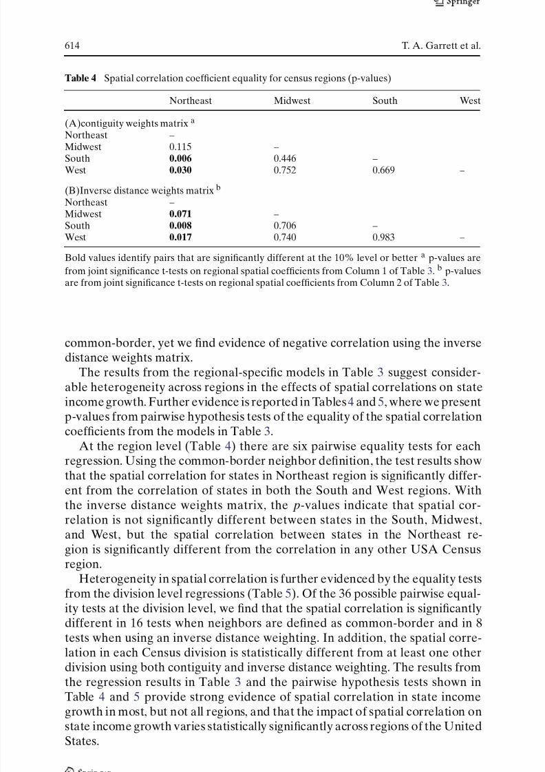
Table 4 Spatial correlation coefficient equality for census regions (p-values)

Northeast Midwest South West

(A)contiguity weights matrix a

Northeast –Midwest 0.115 –South 0.006 0.446 –West 0.030 0.752 0.669 –

(B)Inverse distance weights matrix b

Northeast –Midwest 0.071 –South 0.008 0.706 –West 0.017 0.740 0.983 –

Bold values identify pairs that are significantly different at the 10% level or better a p-values are

from joint significance t-tests on regional spatial coefficients from Column 1 of Table 3. b p-valuesare from joint significance t-tests on regional spatial coefficients from Column 2 of Table 3.

common-border, yet we find evidence of negative correlation using the inversedistance weights matrix.

The results from the regional-specific models in Table 3 suggest consider-able heterogeneity across regions in the effects of spatial correlations on state

income growth. Further evidence is reported in Tables4 and 5, where we presentp-values from pairwise hypothesis tests of the equality of the spatial correlationcoefficients from the models in Table 3.

At the region level (Table 4) there are six pairwise equality tests for eachregression. Using the common-border neighbor definition, the test results showthat the spatial correlation for states in Northeast region is significantly differ-ent from the correlation of states in both the South and West regions. Withthe inverse distance weights matrix, the p-values indicate that spatial cor-relation is not significantly different between states in the South, Midwest,

and West, but the spatial correlation between states in the Northeast re-gion is significantly different from the correlation in any other USA Censusregion.

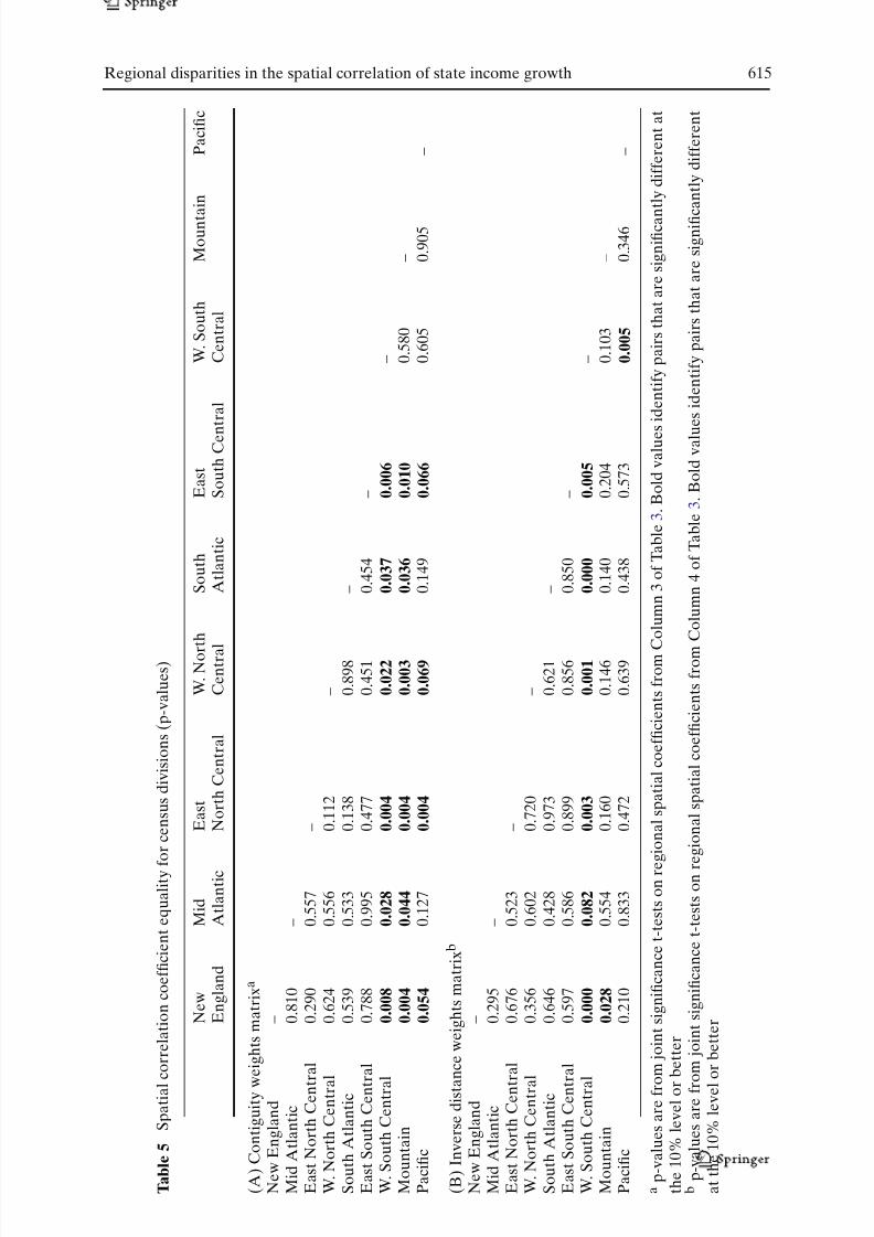
Heterogeneity in spatial correlation is further evidenced by the equality testsfrom the division level regressions (Table 5). Of the 36 possible pairwise equal-ity tests at the division level, we find that the spatial correlation is significantlydifferent in 16 tests when neighbors are defined as common-border and in 8tests when using an inverse distance weighting. In addition, the spatial corre-lation in each Census division is statistically different from at least one otherdivision using both contiguity and inverse distance weighting. The results fromthe regression results in Table 3 and the pairwise hypothesis tests shown inTable 4 and 5 provide strong evidence of spatial correlation in state income




S p a t i a l c o r r e l a t i o n c o e f fi c i e n t e q u a l i t y f o r c e n s u s d i v i s i o n s ( p - v a l u e s )

N e w

M i d

E a s t

W . N o r t h

S o u t h

E a s t

W . S o u t h

M o u n t a i n

P a c i fi c

E n g l a n d

A t l a n t i c

N o r t h C e n t r a l

C e n t r a l

A t l a n t i c

S o u t h C e n

t r a l

C e n t r a l

g u i t y w

e i g h t s m a t r i x a

a n d

–

n t i c

0 . 8 1 0

–

h C e n t r a l

0 . 2 9 0

0 . 5 5 7

–

C e n t r a l

0 . 6 2 4

0 . 5 5 6

0 . 1 1 2

–

a n t i c

0 . 5 3 9

0 . 5 3 3

0 . 1 3 8

0 . 8 9 8

–

h C e n t r a l

0 . 7 8 8

0 . 9 9 5

0 . 4 7 7

0 . 4 5 1

0 . 4 5 4

–

C e n t r a l

0 . 0

0 8

0 . 0

2 8

0 . 0

0 4

0 . 0

2 2

0 . 0

3 7

0 . 0

0 6

–

0 . 0

0 4

0 . 0

4 4

0 . 0

0 4

0 . 0

0 3

0 . 0

3 6

0 . 0

1 0

0 . 5 8 0

–

0 . 0

5 4

0 . 1 2 7

0 . 0

0 4

0 . 0

6 9

0 . 1 4 9

0 . 0

6 6

0 . 6 0 5

0 . 9 0 5

–

e d i s t a

n c e w e i g h t s m a t r i x b

a n d

–

n t i c

0 . 2 9 5

–

h C e n t r a l

0 . 6 7 6

0 . 5 2 3

–

C e n t r a l

0 . 3 5 6

0 . 6 0 2

0 . 7 2 0

–

a n t i c

0 . 6 4 6

0 . 4 2 8

0 . 9 7 3

0 . 6 2 1

–

h C e n t r a l

0 . 5 9 7

0 . 5 8 6

0 . 8 9 9

0 . 8 5 6

0 . 8 5 0

–

C e n t r a l

0 . 0

0 0

0 . 0

8 2

0 . 0

0 3

0 . 0

0 1

0 . 0

0 0

0 . 0

0 5

–

0 . 0

2 8

0 . 5 5 4

0 . 1 6 0

0 . 1 4 6

0 . 1 4 0

0 . 2 0 4

0 . 1 0 3

–

0 . 2 1 0

0 . 8 3 3

0 . 4 7 2

0 . 6 3 9

0 . 4 3 8

0 . 5 7 3

0 . 0

0 5

0 . 3 4 6

–

a r e f r o

m j o i n t s i g n i fi c a n c e t - t e s t s o n r e

g i o n a l s p a t i a l c o e f fi c i e n t s f r o m C

o l u m n 3 o f T a b l e 3 . B o l d v a l u e s i d e n t i f y p a i r s t h a t a r e s i g n i fi c a n

t l y d i f f e r e n t a t

e v e l o r

b e t t e r

a r e f r o m j o i n t s i g n i fi c a n c e t - t e s t s o n r e g i o n a l s p a t i a l c o e f fi c i e n t s f r o m

C o l u m n 4 o f T a b l e 3 . B o l d v a l u

e s i d e n t i f y p a i r s t h a t a r e s i g n i fi c a n t l y d i f f e r e n t

% l e v e l

o r b e t t e r




5 Conclusion

Although the role of space as a determinant of growth has received consider-able attention in recent empirical studies, work in this area has focused almost

exclusively on testing convergence hypotheses using international data. In thispaper we estimate several spatial econometric models to explore the extent of spatial correlation in the short-run growth dynamics of state personal income inthe United States. We use an established set of control variables that are robustdeterminants of state-level growth to reduce the possibility that any uncoveredspatial patterns are the result of omitted variable bias or measurement issues.

Our results provide strong evidence that spatial correlation exists in state-level income growth. The models in which we assume a common spatial lagcoefficient for all states, we find that a 1% point increase in the average income

growth of “neighboring” states generates between a 0.22 and 0.29 increase in agiven state’s income growth rate, depending on the specification. In addition,this paper is the first to explore whether spatial correlation in state incomegrowth varies for states in different regions of the USA. We find that spatialcorrelation in state income growth does differ significantly by region, and ourmodel of regional-specific spatial correlations fits the data better than the typ-ical spatial econometric model that assumes a common spatial lag coefficientfor all regions. Generally, we find that states in the Northeast and South experi-ence the strongest cross-state income linkages—roughly a 0.20–0.40% increase

in state income growth for every percentage point increase in ‘neighboring’state income growth. States in these regions are generally smaller and morepopulous, and thus are more likely to have linked economies, than states in theMidwest and western regions of the country.

The broader implication of our findings is that the spatial correlations atwork in income growth dynamics appear to be complex. Further research iswarranted to improve our understanding of how various regional forces affectgrowth dynamics and to uncover the underlying source(s) of such regionalforces. Our results suggest that states should pay particular attention to fiscal

policies in neighboring states, as state-level fiscal policies can significantly influ-ence income growth in neighboring states. For example, Tomljanovich (2004)finds that state taxes in general, and corporate income taxes specifically, havea negative transitory effect on state growth. The composition of governmentspending is also found to affect short-term growth, with public assistance spend-ing slowing growth and other forms of government spending generally enhanc-ing short-term growth. Thus, our results suggest if one state alters tax rates orthe composition of government spending, then neighboring states, primarily inthe central and eastern regions of the USA, will also experience the growtheffects of these choices. And given Poterba’s (1994) finding that state policymakers make larger fiscal adjustments during periods of unexpected budgetdeficits, the overall fiscal condition of neighboring states may have sizable own-




counties in different states with whom the county shares a common border.They find consistent and strong evidence that tax increases in these “matched”counties reduces growth in neighboring counties. Given the strength of ourresults, a study similar to Holcombe and Lacombe (2004) among regions at the

state level may be particularly fruitful.In addition, policy makers should realize that exogenous shocks in neigh-

boring states that improve or deteriorate economic conditions are also likelyto affect economic growth in their own states. There are numerous poten-tial “shocks”, with recent examples being the 9/11 terrorist attacks, HurricaneKatrina, and rising energy prices. In the case of the 9/11 attacks for instance, theyhad widespread consequences that influenced several industries andextended well beyond New York City and Washington, D.C. (Bonham et al.2006, Makinen 2002). And, as Brown and Yucel (1995) note, energy-producing

states such as TX are particularly sensitive to industry-specific shocks and ourresults imply that these shocks could translate into considerable growth effectsin neighboring states.

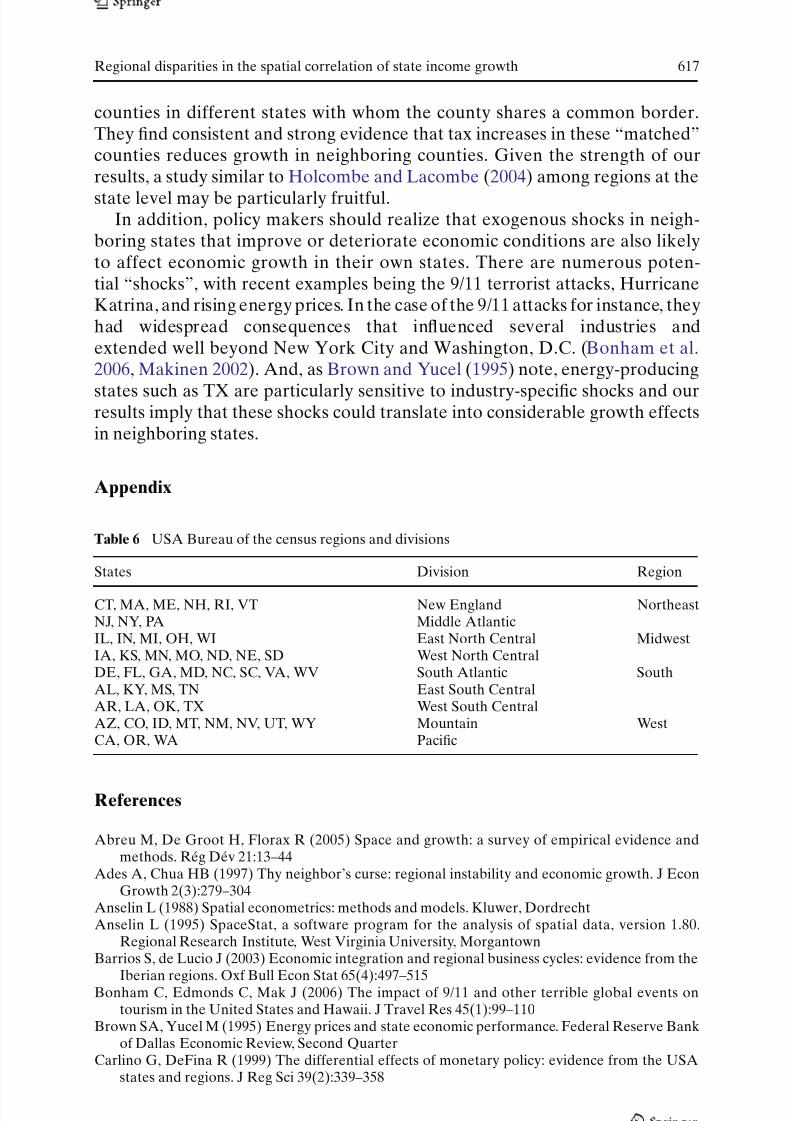
Appendix

Table 6 USA Bureau of the census regions and divisions

States Division Region

CT, MA, ME, NH, RI, VT New England NortheastNJ, NY, PA Middle AtlanticIL, IN, MI, OH, WI East North Central MidwestIA, KS, MN, MO, ND, NE, SD West North CentralDE, FL, GA, MD, NC, SC, VA, WV South Atlantic SouthAL, KY, MS, TN East South CentralAR, LA, OK, TX West South CentralAZ, CO, ID, MT, NM, NV, UT, WY Mountain WestCA, OR, WA Pacific

References

Abreu M, De Groot H, Florax R (2005) Space and growth: a survey of empirical evidence andmethods. Rég Dév 21:13–44

Ades A, Chua HB (1997) Thy neighbor’s curse: regional instability and economic growth. J EconGrowth 2(3):279–304

Anselin L (1988) Spatial econometrics: methods and models. Kluwer, DordrechtAnselin L (1995) SpaceStat, a software program for the analysis of spatial data, version 1.80.

Regional Research Institute, West Virginia University, MorgantownBarrios S, de Lucio J (2003) Economic integration and regional business cycles: evidence from the

Iberian regions. Oxf Bull Econ Stat 65(4):497–515Bonham C, Edmonds C, Mak J (2006) The impact of 9/11 and other terrible global events ontourism in the United States and Hawaii. J Travel Res 45(1):99–110




Carlino G, Sill K (2001) Regional income fluctuations: common trends and common cycles. RevEcon Stat 83(3):446–456

Case A (1992) Neighborhood influence and technological change. Reg Sci Urban Econ 22(3):491–508

Cliff A, Ord J (1981) Spatial processes: models and applications. Pion, London

Conley TG, Ligon E(2002) Economic distance and cross-country spillovers. J Econ Growth7(2):157–187

Crain WM, Lee KJ (1999) Economic growth regressions for the American states: a sensitivityanalysis. Econ Inq 37(2):242–257

DeJuan J, Tomljanovich M (2005) Income convergence across Canadian provinces in the 20thcentury: almost but not quite there. Ann Reg Sci 39(3):567–592

DeLong JB, Summers LH (1991) Equipment investment and economic growth. Q J Econ106(2):445–502

Dubin RA (1988) Estimation of regression coefficients in the presence of spatially correlated Terms.Rev Econ Stat 70(3):466–474

Fingleton B (2001) Equilibrium and economic growth: spatial econometric models and simulations.

J Reg Sci 41(1):117–147Freeman DG (2002) Did state bank branching deregulation produce large growth effects. EconLett 75(3):383–389

Freeman DG (2005) Change-point analysis of the growth effects of state banking deregulation.Econ Inq 43(3):601–613

Garrett TA, Marsh TL (2002) The revenue impacts of cross-border lottery shopping in the presenceof spatial autocorrelation. Reg Sci Urban Econ 32(4):501–519

Garrett TA, Wagner GA, Wheelock DC (2005) A spatial analysis of state banking regulation. PapReg Sci 84(4):575–595

Holcombe RG, Lacombe D (2004) The effect of state income taxation on per capita income growth.Public Finance Rev 32(3):292–312

Hernandez R(2003) Strategic interaction in tax policies among states. Fed Reserve Bank St Louis

Rev 85(3):47–56Jayaratne J, Strahan PE (1996) The finance-growth nexus: evidence from bank branch deregulation.

Q J Econ 111(3):639–670Krol R, Svorny S (1996) The effect of bank regulatory environment on state economic activity. Reg

Sci Urban Econ 26(5):531–541Kroszner RS, Strahan PE (1999) What drives deregulation? Economics andpolitics of therelaxation

of bank branching restrictions. Q J Econ 114(4):1437–1466Le Gallo J (2004) Space-time analysis of GDP disparities among European regions: a markov

chains approach. Int Reg Sci Rev 27(2):138–163Makinen G (2002) The economic effects of 9/11: a retrospective assessment. Congressional

Research Service, Washington, DCMoreno R, Trehan B (1997) Location and the growth of nations. J Econ Growth 2(4):399–418Poterba J (1994) State responses to fiscal crises: the effects of budgetary institutions and politics.

J Pol Econ 102(4):799–821Quah D (1993) Empirical cross-section dynamics in economic growth. Eur Econ Rev 37(2–3):

426–434Quah D (1996) Empirics for economic growth and convergence. Eur Econ Rev 40(6):1353–1375Ramirez MT, Loboguerrero AM (2002) Spatial correlation and economic growth: evidence from a

panel of countries. Working paper no. 206, Central Bank of CA, BogotaRey SJ, Montouri BD (1999) USA regional income convergence: a spatial econometric perspective.

Reg Stud 33(2):143–156Strahan P (2003) The real effects of USA banking deregulation. Fed Reserve Bank St Louis Rev

85(4):111–128

Tomljanovich M (2004) The role of state fiscal policy in state economic growth. ContemporaryEcon Policy 22(3):318–330Wheelock DC (2003) Commentary on the real effects of USA Banking deregulation. Fed Reserve



Reproducedwithpermissionof thecopyrightowner. Further reproductionprohibitedwithoutpermission.

Documents

Regional Disparities in the Spatial Correlation of State Income Growth