Embed Size (px)
Citation preview

AnalysisAttila Bérczes
Attila Gilányi
Created by XMLmind XSL-FO Converter.

AnalysisAttila BérczesAttila Gilányi
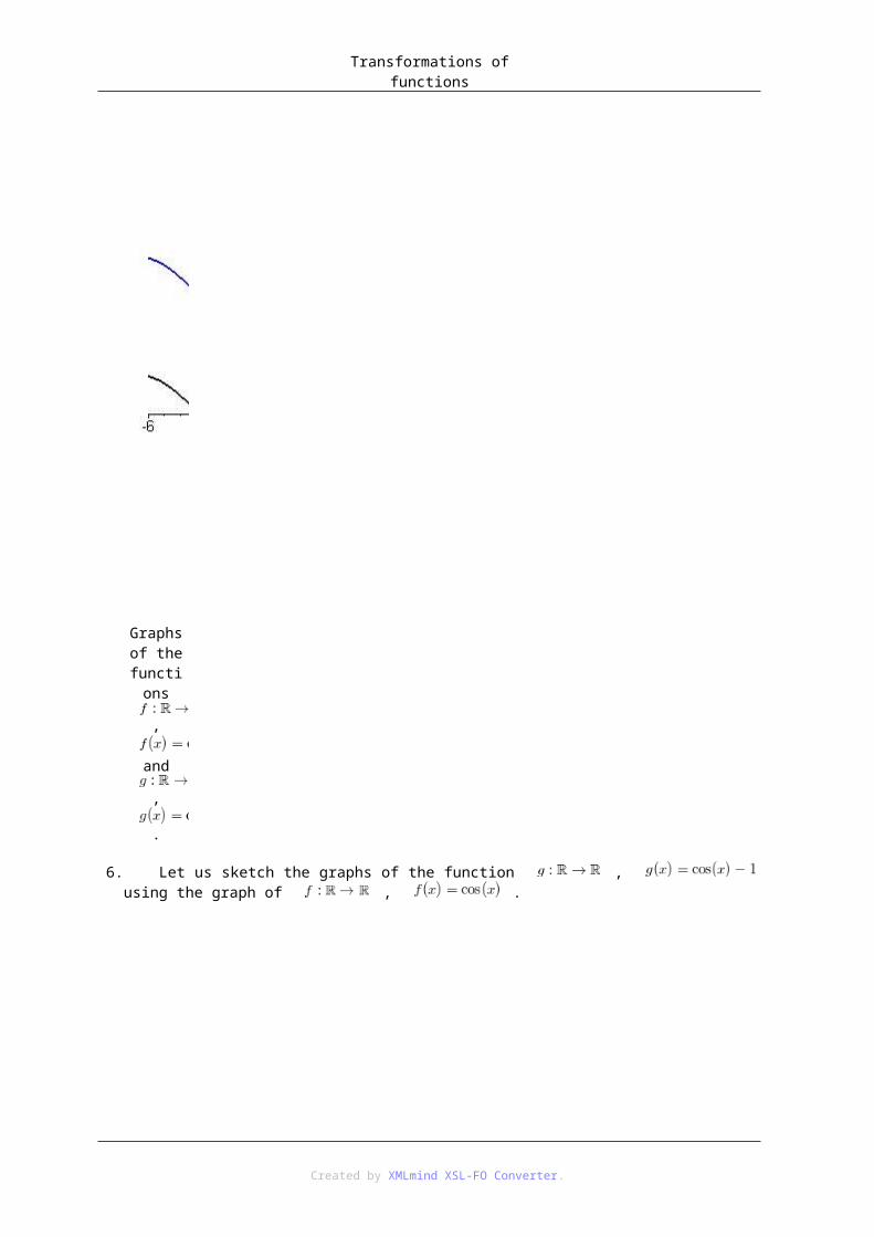
Debreceni Egyetem
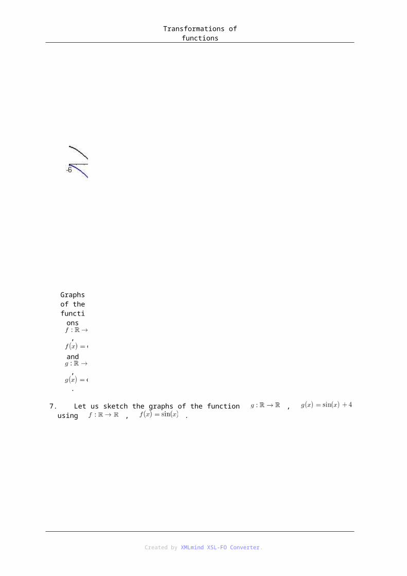
Reviewer
Dr. Attila Házy
University of Miskolc, Institute of Mathematics, Department of Applied Mathematics
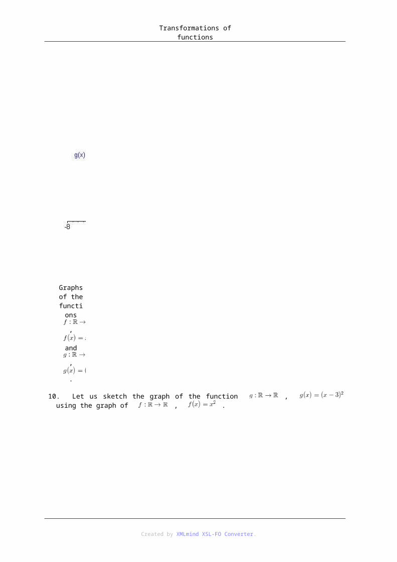
The curriculum granted / supported by the Hungarian Scientific Research Fund (OTKA) Grant NK-81402 and by the TÁMOP-4.1.2.A/1-11/1-2011-0098 and TÁMOP 4.2.2.C-11/1/KONV-2012-0001 projects.
Created by XMLmind XSL-FO Converter.

Table of ContentsIntroduction .......................................................................................................................................... 51. The concept and basic properties of functions ................................................................................. 1
1. 1.1. Relations and functions ................................................................................................... 12. 1.2. A `friendly' introduction to functions .............................................................................. 33. 1.3. The graph of a function ................................................................................................... 6
3.1. 1.3.1. Cartesian coordinate system ............................................................................ 63.2. 1.3.2. The graph of a function .................................................................................... 73.3. 1.3.3. The graph of equations or relations ................................................................. 93.4. 1.3.4. The vertical line test ....................................................................................... 103.5. 1.3.5. The -intercept and the -intercepts of functions ......................... 13
4. 1.4. New functions from old ones ........................................................................................ 155. 1.5. Further properties of functions ...................................................................................... 22
5.1. 1.5.1. Injectivity of functions ................................................................................... 225.2. 1.5.2. Surjectivity of functions ................................................................................ 275.3. 1.5.3. Bijectivity of functions .................................................................................. 335.4. 1.5.4. Inverse of a function ...................................................................................... 43
2. Types of functions .......................................................................................................................... 561. 2.1. Linear functions ............................................................................................................. 562. 2.2. Quadratic functions ....................................................................................................... 603. 2.3. Polynomial functions ..................................................................................................... 65
3.1. 2.3.1. Definition of polynomial functions ............................................................... 653.2. 2.3.2. Euclidean division of polynomials in one variable ....................................... 653.3. 2.3.3. Computing the value of a polynomial function ............................................. 67
4. 2.4. Power functions ............................................................................................................. 695. 2.5. Exponential functions .................................................................................................... 706. 2.6. Logarithmic functions ................................................................................................... 72
3. Trigonometric functions ................................................................................................................. 751. 3.1. Measures for angles: Degrees and Radians ................................................................... 752. 3.2. Rotation angles .............................................................................................................. 763. 3.3. Definition of trigonometric functions for acute angles of right triangles ..................... 77
3.1. 3.3.1. The basic definitions ...................................................................................... 773.2. 3.3.2. Basic formulas for trigonometric functions defined for acute angles ........... 793.3. 3.3.3. Trigonometric functions of special angles ..................................................... 80
4. 3.4. Definition of the trigonometric functions over .................................................. 825. 3.5. The period of trigonometric functions .......................................................................... 836. 3.6. Symmetry properties of trigonometric functions .......................................................... 847. 3.7. The sign of trigonometric functions .............................................................................. 858. 3.8. The reference angle ....................................................................................................... 879. 3.9. Basic formulas for trigonometric functions defined for arbitrary angles ...................... 90
9.1. 3.9.1. Cofunction formulas ...................................................................................... 909.2. 3.9.2. Quotient identities .......................................................................................... 909.3. 3.9.3. The trigonometric theorem of Pythagoras ..................................................... 91
10. 3.10. Trigonometric functions of special rotation angles ................................................... 9111. 3.11. The graph of trigonometric functions ........................................................................ 91
11.1. 3.11.1. The graph of ............................................................................... 9111.2. 3.11.2. The graph of ............................................................................... 9211.3. 3.11.3. The graph of .............................................................................. 92
Created by XMLmind XSL-FO Converter.

Analysis
11.4. 3.11.4. The graph of ............................................................................... 9312. 3.12. Sum and difference identities .................................................................................... 94
12.1. 3.12.1. Sum and difference identities of the function and .......... 9412.2. 3.12.2. Sum and difference identities of the function and .......... 96
13. 3.13. Multiple angle identities ............................................................................................ 9713.1. 3.13.1. Double angle identities .............................................................................. 9713.2. 3.13.2. Triple angle identities ................................................................................ 99
14. 3.14. Half-angle identities ................................................................................................ 10015. 3.15. Product-to-sum identities ........................................................................................ 10116. 3.16. Sum-to-product identities ........................................................................................ 102
4. Transformations of functions ....................................................................................................... 1051. 4.1. Shifting graphs of functions ........................................................................................ 1052. 4.2. Scaling graphs of functions ......................................................................................... 134
5. Results of the exercises ................................................................................................................ 1751. 5.1. Results of the Exercises of Chapter 1 ......................................................................... 1752. 5.2. Results of the Exercises of Chapter 2 ......................................................................... 2273. 5.3. Results of the Exercises of Chapter 3 ......................................................................... 240
Bibliography .................................................................................................................................... 242
Created by XMLmind XSL-FO Converter.

IntroductionThis textbook contains the knowledge expected to be acquired by the students at the "College Functions" class of the Foundation Year and Intensive Foundation Semester at the University of Debrecen.
We have tried to compose the textbook such that it is a self-contained material, including many examples, figures and graphs of functions which help the students in better understanding the topic, however, this book is primarily meant to be used as a Lecture Notes connected to the "College Analysis" class. Thus we suggest the students to attend the classes, and use this book as a supplementary mean of study.
In Chapter 1 we define the basic concepts connected to functions, and the most important properties of functions which we shall analyze later in the case of many types of functions.
In Chapter 2 we present some basic types of functions, like linear functions, quadratic functions, polynomial functions, power functions, exponential and logarithmic functions, along with their most important properties.
Chapter 3 is devoted to a detailed description of trigonometric functions.
The topic of Chapter 4 is the transformation of functions.
The last Chapter contains the results of the unsolved exercises of the book, which will help the students to check if their solutions lead to the right answer or not.
This work has been supported by the Hungarian Scientific Research Fund (OTKA) Grant NK-81402 and by the TÁMOP-4.1.2.A/1-11/1-2011-0098 and TÁMOP 4.2.2.C-11/1/KONV-2012-0001 projects.
These projects have been supported by the European Union, co-financed by the European Social Fund.
Attila Bérczes and Attila Gilányi
Created by XMLmind XSL-FO Converter.

Chapter 1. The concept and basic properties of functions1. 1.1. Relations and functionsIn this section we provide a precise definition of binary relations and functions, which is the mathematically correct way to introduce these concepts. However, this section is recommended mostly for the interested reader, and we give a less precise but simpler introduction of functions in the next section.
Definition 1.1. Let be a non-empty set and elements of . The ordered pair is defined by
Theorem 1.2. Let and be two ordered pairs. We have
Definition 1.3. Let be two sets. The Cartesian product of and is the set of all ordered pairs with the first element being from and the second element from , i.e.
Definition 1.4. Let be two non-empty sets. A binary relation between and be is a subset of the Cartesian product , i.e. . If then we also say that
• is in relation with , or
• is assigned , or
• assigns to .
If then we say that is a binary relation on .
Notation. For we also use the notation .
Examples. Here we give some examples of binary relations from our earlier mathematical experience:
1. The relation on the set of real numbers.
2. The realtion on the integers.
3. The congruence of triangles.
4. The parallelity of lines in the plane.-
We also give an abstract example to illustrate the definition above:
Let and , .
Definition 1.5. Let be a binary relation. Then
Created by XMLmind XSL-FO Converter.

The concept and basic properties of functions
Definition 1.6. The binary relation is called a function if
The domain and the range of the function are the sets which are defined as the domain and the range of considered as a relation.
Notation. If a relation is a function, then
• instead of we write and we say that is a function from to ;
• instead of writing or we shall write and we say that maps the element to the element , or is the image of by the function .
Remark. The above definition means that a function maps each element of its domain to a well-defined single element of the range.
Example. First we give an example for a function , given by a diagram, where and :
This in fact means that , , and . The domain of is and the range of is .
Example. The following diagram defines a relation from to , where and . However this relation is not a function.
Created by XMLmind XSL-FO Converter.

The concept and basic properties of functions
We have , , , . The domain of is and the range of is . We emphasize that the relation defined by the diagram is not a function, since
for the same we have both and , and this is not allowed in the case of a function.
Example. The following diagram also defines a function from to , where and .
We have , , , . The domain of is and the range of is . We emphasize that the relation defined by
the diagram is a function, although , so two different elements may have the same image by a function.
Remark. We wish to emphasize the difference between the two last examples. In the last example is a function, even if is the image of two different elements of . On the other hand in the preceding example is not a function since assigns two different elements to .
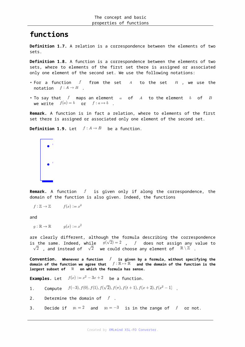
2. 1.2. A `friendly' introduction to functionsDefinition 1.7. A relation is a correspondence between the elements of two sets.
Definition 1.8. A function is a correspondence between the elements of two sets, where to elements of the first set there is assigned or associated only one element of the second set. We use the following notations:
• For a function from the set to the set , we use the notation .
• To say that maps an element of to the element of we write or .
Created by XMLmind XSL-FO Converter.
The concept and basic properties of functions
Remark. A function is in fact a relation, where to elements of the first set there is assigned or associated only one element of the second set.
Definition 1.9. Let be a function.
Remark. A function is given only if along the correspondence, the domain of the function is also given. Indeed, the functions
and
are clearly different, although the formula describing the correspondence is the same. Indeed, while , does not assign any value to , and instead of we could choose any
element of .
Convention. Whenever a function is given by a formula, without specifying the domain of the function we agree that and the domain of the function is the largest subset of on which the formula has sense.
Examples. Let be a function.
1. Compute .
2. Determine the domain of .
3. Decide if and is in the range of or not.
4. Determine the range of .
Solution.
1. To compute the value of the function given by the formula taken at a number or expression we substitute every occurrence of in the right hand side of the formula defining by the
number or expression .
Created by XMLmind XSL-FO Converter.

The concept and basic properties of functions
2. To determine the (maximal) domain of the function given by a formula we have to determine the maximal subset of on which the formula defining has sense. Since has sense for every real number the (maximal) domain of is the whole set of real numbers, i.e.
.
3. To decide if a concrete number belongs to range of a function given by a formula we need to solve the equation in the variable , where is a given number. If the equation has a solution in the domain of then belongs to the range of , otherwise does not belong to the range of .
To decide if is in the range of or not we have to check if the equation
has a solution in or not. So we solve the equation
We obtain that
thus,
Since
we see that .
To decide if is in the range of or not we have to check if the equation
has a solution in or not. So we solve the equation
Since the discriminant the above equation has no solution and we see that .
4. To determine the range of a function given by a formula we need to solve the equation in the variable , where is a parameter. The range of of consists of those values
, for which the equation has a solution in the domain of .
Created by XMLmind XSL-FO Converter.

The concept and basic properties of functions
Thus we shall check for which values of the parameter the equation
has a solution in . The equation takes the form
which has a solution if and only if its discriminant is non-negative, i.e.
This is equivalent to , so the range of is .
Exercise 1.1. Let be one of the functions below.
a) Compute .
b) Determine the domain of .
c) Decide if and (given below next to the function ) is in the range of or not.
d) Determine the range of .
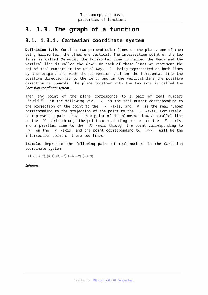
3. 1.3. The graph of a function3.1. 1.3.1. Cartesian coordinate systemDefinition 1.10. Consider two perpendicular lines on the plane, one of them being horizontal, the other one vertical. The intersection point of the two lines is called the origin, the horizontal line is called the X-axis and the vertical line is called the Y-axis. On each of these lines we represent the set of real numbers in the usual way,
being represented on both lines by the origin, and with the convention that on the horizontal line the positive direction is to the left, and on the vertical line the positive direction is upwards. The plane together with the two axis is called the Cartesian coordinate system.
Then any point of the plane corresponds to a pair of real numbers in the following way: is the real number corresponding to the projection of the point to the -axis, and is the real number corresponding to the projection of the point to the -axis. Conversely, to represent a pair as a point of the plane we draw a parallel line to the -axis through the point corresponding to on the
-axis, and a parallel line to the -axis through the point corresponding to on the -axis, and the point corresponding to will be the intersection point of these two lines.
Example. Represent the following pairs of real numbers in the Cartesian coordinate system:
Solution.
Created by XMLmind XSL-FO Converter.
The concept and basic properties of functions
3.2. 1.3.2. The graph of a functionDefinition 1.11. Let be a function. The set
is called the graph of the function .
The graph of a function can be represented in the so-called Cartesian coordinate system.
Graphing a function:
Example. Draw the graph of the function .
1. We compute the pairs for :
2. We plot the points ,
Created by XMLmind XSL-FO Converter.

The concept and basic properties of functions
,
3. We connect the points by a smooth curve
Exercise 1.2. Sketch the graph of the following functions:
Created by XMLmind XSL-FO Converter.

The concept and basic properties of functions
3.3. 1.3.3. The graph of equations or relationsSimilarly to the graph of functions one may represent relations or solutions of an equation in two unknowns in the Cartesian coordinate system.
Example. Represent the set of solutions of the equation
in the Cartesian coordinate system.
Solution. We have to draw the curve corresponding to the set
in the Cartesian system, so we get
Remark. Clearly, the graph of the function is the same as the graph of the equation . Thus, when there is no danger of confusion we shall not make any distinction among them.
Created by XMLmind XSL-FO Converter.
The concept and basic properties of functions
3.4. 1.3.4. The vertical line test
Example. The following two figures show the essential difference between the graph of a function and a curve that is not the graph of a function:
Created by XMLmind XSL-FO Converter.

The concept and basic properties of functions
Remark. The vertical line test is a graphical method, which is very useful to understand well the concept of a function, however, in itself it is not a rigorous proving method. However, if we "see" the vertical line showing that a curve is not the graph of a function, then it is easy to write down the proof rigorously.
Exercise 1.3. Using the vertical line test decide if the following curves are graphs of a function or not:
a)
Created by XMLmind XSL-FO Converter.

The concept and basic properties of functions
b)
c)
Created by XMLmind XSL-FO Converter.

The concept and basic properties of functions
d)
3.5. 1.3.5. The -intercept and the -intercepts of functions
Created by XMLmind XSL-FO Converter.

The concept and basic properties of functions
When drawing the graph of a function we pay special interest to the intersection of the graph with the coordinate axis.
Definition 1.12. (Intercepts of the graph of a function)
• The intersection point of the graph of a function with the -axis is called the -intercept of the graph.
• An intersection point of the graph of a function with the -axis is called an -intercept of the graph.
Remark. Note the difference on the two points of the above definition: the -intercept is a single point (if it exists), however there might exist more -intercepts. Indeed, the vertical line test guarantees that the graph of a function might intersect the -axis (which is a vertical line) in at most one point.
Theorem 1.13. (The -intercept of a function) The graph of a function has -intercept if and only if it is defined in , and it is the point with .
Theorem 1.14. (The -intercepts of a function) The graph of a function given by a formula has -intercepts if and only if the equation
has solutions in the domain of , and the -intercepts are the points for , where for are the solutions of the above equation.
Example. Compute the -intercept and the -intercepts of the graph of the function .
Solution. The intercept is the point , i.e. the point (since ).
The -intercepts are the points having -coordinate zero, their -coordinates being the solutions of the equation
Using the "Almighty formula" these solutions are and , so the -intercepts are and .
Exercise 1.4. Compute the -intercept and the -intercepts of the following functions:
Created by XMLmind XSL-FO Converter.
The concept and basic properties of functions
4. 1.4. New functions from old onesDefinition 1.15. (The sum, difference, product and quotient of functions) Let be two functions defined by the formulas and , and denote by and the domain of
and , respectively. Put and . Then
• the sum of and is defined by
• the difference of and is defined by
• the product of and is defined by
• the quotient of and is defined by
Remark. The above definition means that the sum, difference, product and quotient of two functions given by a formula is the function defined by the sum, difference, product and quotient of the two formulas, however, the domain is not the maximal domain implied by the resulting formula, but the intersection of the domains of the original functions, or in case of the quotient, an even more restricted set.
For example if and then , and thus
even if the function defined simply by the formula would have maximal domain .
Example. Let be two functions given by and . Then we have
Definition 1.16. (Composition of functions) Let and two functions such that , where denotes the range of and the domain of . Then the composite
function is defined as
for every in the domain of .
Remark. The composition of functions may also be regarded as connecting two machines. Namely, the first machine transforms the input to the output , which will be the input of the machine , and this transforms to . Then the "connected machine" is the machine which transforms the input to , and we already cannot see which part of the "work" was done by the machines and , respectively.
Created by XMLmind XSL-FO Converter.

The concept and basic properties of functions
Remark. In most cases we shall work with composite functions in the case , so the composite functions and can be both defined. However, these functions in general are different, i.e. the composition of functions is not commutative.
Example. Let , and . Then
Exercise 1.5. Compute , , , , and , provided that
Example. Let and for . Let and for and . Further, let , and
. Build the following function as a composite function of the above functions:
Solution.
Exercise 1.6. Let and for . Let and for and . Further, let , and
. Build the following function as a composite function of the above functions:
Created by XMLmind XSL-FO Converter.

The concept and basic properties of functions
Definition 1.17. Let , and be sets, and let be a function. The function , for which for each , is said to be the restriction of to the set
.
The restriction of the function to the set is also denoted by .
Examples.
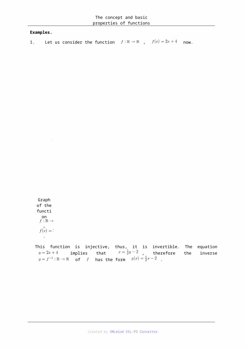
1. Let us consider the function , . The graph of is:
Graph of the
function
Created by XMLmind XSL-FO Converter.
The concept and basic properties of functions
,
.
The restriction of to the set is , . The graph of is:
Graph of the
function
,
.
2. Let , . The graph of is:
Created by XMLmind XSL-FO Converter.

The concept and basic properties of functions
Graph of the
function
,
.
The restriction of to the set is , . The graph of is:
Created by XMLmind XSL-FO Converter.

The concept and basic properties of functions
Graph of the
function
,
.
The restriction of to the set is , . The graph of is:
Created by XMLmind XSL-FO Converter.
The concept and basic properties of functions
Graph of the
function
,
.
The restriction of to the set is , . The graph of is:
Created by XMLmind XSL-FO Converter.

The concept and basic properties of functions
Graph of the
function
,
.
5. 1.5. Further properties of functions5.1. 1.5.1. Injectivity of functionsDefinition 1.18. Let and arbitrary sets. A function is called injective if, for all
, for which and , we have .
Remark. Injective functions are also called invertible.
Examples.
1. Let , and let us define such that , , , . It is easy to see that satisfies the requirements given in
Definition 1.6 [2], therefore, it is a function. It can be illustrated in the following form:
Created by XMLmind XSL-FO Converter.

The concept and basic properties of functions
It is visible, that there are no elements and such that , which implies that is injective.
2. Let now , and let , , , , . This function can be illustrated as
It is easy to see that is a function, but, since , it is not injective.
3. Let us consider the function , . The graph of this function has the following form.
Created by XMLmind XSL-FO Converter.

The concept and basic properties of functions
Graph of the
function
,
.
It is easy to see, that there are no elements and such that , which yields the injectivity of .
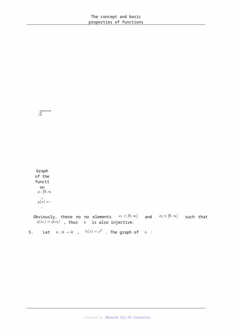
4. Let , . The graph of is:
Created by XMLmind XSL-FO Converter.

The concept and basic properties of functions
Graph of the
function
,
.
Obviously, there no no elements and such that , thus is also injective.
5. Let , . The graph of :
Created by XMLmind XSL-FO Converter.

The concept and basic properties of functions
Graph of the
function
,
.
Since there are elements , such that (for example ), the function is not injective.
6. Let us consider the function , now. The graph of is:
Created by XMLmind XSL-FO Converter.
The concept and basic properties of functions
Graph of the
function
,
.
Obviously, there does not exist elements and such that , therefore is an injective function.
Remark. The last two examples point out that if we investigate the injectivity of a function then the domain of the function plays an important role.
5.2. 1.5.2. Surjectivity of functionsDefinition 1.19. Let and arbitrary sets. A function is said to be surjective if the range of is .
Remark. The definition above requires that, for each , there exists an such that .
Examples.
1. Let , and let such that , , , , i.e.,
Created by XMLmind XSL-FO Converter.

The concept and basic properties of functions
It is visible that is a function, furthermore, it is also clear that, for each element , there exists an such that , therefore is surjective.
2. Let now , and let , , , , . A diagram corresponding to is:
It is easy to see that is a function. However, there exists an element such that there is no for which . (The element has this property.) This implies that is
not surjective.
3. Let us consider the function , . The graph of this function has the following form.
Created by XMLmind XSL-FO Converter.

The concept and basic properties of functions
Graph of the
function
,
.
It is easy to verify that, for each there exists an for which . (Solving the equation for , we obtain such an for each .) This means that the function is surjective.
4. Let , . The graph of is:
Created by XMLmind XSL-FO Converter.

The concept and basic properties of functions
Graph of the
function
,
.
Since there are elements in the range of such that there is no element in the domain of for which . (For example fulfills this property.) Therefore
is not surjective.
5. Let , . The graph of is:
Created by XMLmind XSL-FO Converter.

The concept and basic properties of functions
Graph of the
function
,
.
It is easy to see that, for each there exists an such that Thus, is surjective.
6. Let , . The graph of :
Created by XMLmind XSL-FO Converter.

The concept and basic properties of functions
Graph of the
function
,
.
It is easy to check that is not surjective.
7. Let , . The graph of :
Created by XMLmind XSL-FO Converter.

The concept and basic properties of functions
Graph of the
function
,
.
It is obvious that is surjective.
Remark. The last four examples show that concerning the injectivity of a function the range of the function plays an important role.
5.3. 1.5.3. Bijectivity of functionsDefinition 1.20. Let and arbitrary sets. A function is called bijective if it is injective and surjective.
Examples.
1. Let , and let , , , , . It is easy to see that is a function, furthermore, it is injective
and surjective, therefore, it is bijective. The function has the diagram
Created by XMLmind XSL-FO Converter.

The concept and basic properties of functions
2. Let , and let , , , , . This function is injective but not surjective, thus, it is not bijective. An
illustration of is:
3. Let , and let , , , , . The function is surjective but not injective, which yields that it
is not bijective. The function can be illustrated in the following form:
Created by XMLmind XSL-FO Converter.

The concept and basic properties of functions
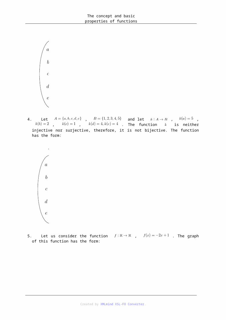
4. Let , and let , , , , . The function is neither injective nor surjective, therefore, it is
not bijective. The function has the form:
5. Let us consider the function , . The graph of this function has the form:
Created by XMLmind XSL-FO Converter.

The concept and basic properties of functions
Graph of the
function
,
.
It is easy to see that this function is injective and surjective, therefore, it is bijective.
6. Let us consider the function , . The graph of g is:
Created by XMLmind XSL-FO Converter.
The concept and basic properties of functions
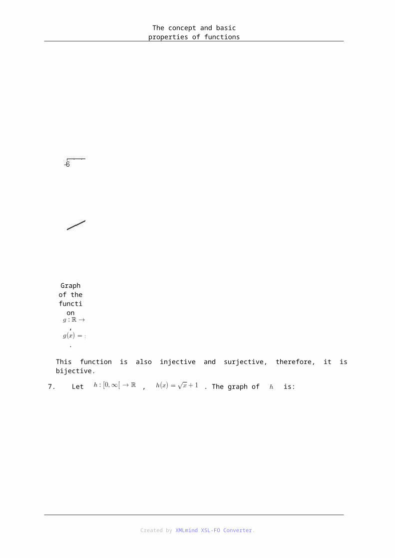
Graph of the
function
,
.
This function is also injective and surjective, therefore, it is bijective.
7. Let , . The graph of is:
Created by XMLmind XSL-FO Converter.

The concept and basic properties of functions
Graph of the
function
,
.
The function is injective but not surjective, thus, it is not bijective.
8. Let , . The graph of is:
Created by XMLmind XSL-FO Converter.
The concept and basic properties of functions
Graph of the
function
,
.
The function is injective and surjective, therefore, it is bijective.
9. Let , . The graph of :
Created by XMLmind XSL-FO Converter.

The concept and basic properties of functions
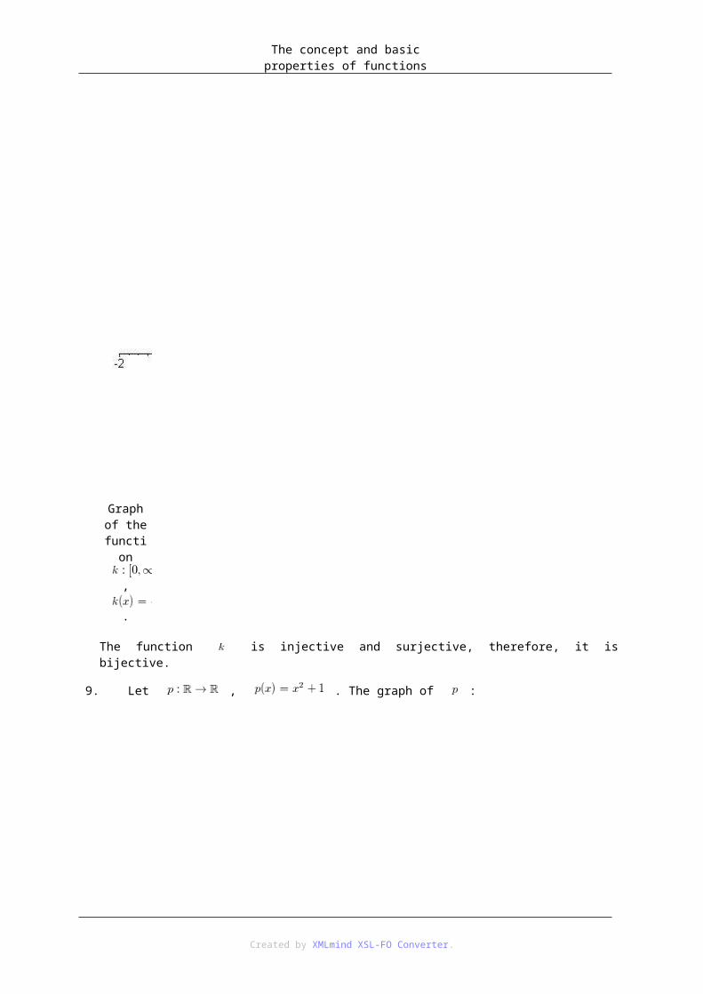
Graph of the
function
,
.
This function is neither injective nor surjective, thus, it is not bijective.
10. Let , . The graph of :
Created by XMLmind XSL-FO Converter.
The concept and basic properties of functions
Graph of the
function
,
.
The function is injective but not surjective, therefore, it is not bijective.
11. Let , . The graph of :
Created by XMLmind XSL-FO Converter.

The concept and basic properties of functions
Graph of the
function
,
.
The function is injective and surjective, thus, it is bijective.
Remark. The examples above show that concerning the bijectivity of a function its domain and its range is also important.
Exercise 1.7. Illustrate the following functions and decide whether they are bijective, injective or surjective:
a) , ,
, , , , , ;
b) , ,
, , , , , ;
c) , ,
, , , , ;
d) , ,
, , , , , ;
Created by XMLmind XSL-FO Converter.

The concept and basic properties of functions
e) , ,
, , , , , ;
f) , ,
, , , , , .
Exercise 1.8. Draw the graph of the following functions in a coordinate system and decide whether they are bijective, injective or surjective:
a) , ;
b) , ;
c) , ;
d) , ;
e) , ;
f) , ;
g) , ;
h) , ;
i) , ;
j) , ;
k) , ;
l) , .
5.4. 1.5.4. Inverse of a functionDefinition 1.21. Let and arbitrary sets, let be a injective function and let us denote the range of by . Interchanging the elements in the ordered pairs , we obtain a function , . This function is said to be the inverse function of .
The inverse function of is denoted by .
Remark. It is important to note that the inverse function is defined in the case of injective functions only.
Examples.
1. Let , and let us define , , , , . This function can be illustrated as:
Created by XMLmind XSL-FO Converter.
The concept and basic properties of functions
It is easy to see that this function is injective, thus there exists its inverse. The inverse of has the form
that is,
Created by XMLmind XSL-FO Converter.

The concept and basic properties of functions
which means that , , , and .
2. Let , and let us define , , , , . This function can be illustrated as:
The function is injective, therefore, it is invertible. It is important to mention, that the range of is the set , which means that the domain of will be this set, too. Thus,
, , , , , that is,
Created by XMLmind XSL-FO Converter.

The concept and basic properties of functions
3. Let , and let , , , , , i. e.,
The function is not injective, thus, it does not have any inverse.
4. Let us consider the function , . The graph of this function has the form:
Created by XMLmind XSL-FO Converter.

The concept and basic properties of functions
Graph of the
function
,
.
This function is injective, therefore, it is invertible. Its inverse can be determined in the following form: by the definition of , we may write for all , which means that for each
. Therefore, the inverse of can be written as or, writing instead of , . The graph of
is:
Created by XMLmind XSL-FO Converter.

The concept and basic properties of functions
Graph of the
function
,
.
Let us draw the graphs of the functions and above in the same coordinate system.
Created by XMLmind XSL-FO Converter.

The concept and basic properties of functions
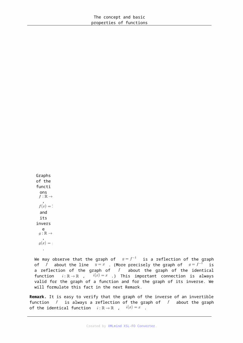
Graphs of the
functions
,
and its inverse
,
.
We may observe that the graph of is a reflection of the graph of about the line . (More precisely the graph of is a reflection of the graph of about the graph of the identical function , .) This important connection is always valid for the graph of a function and for the graph of its inverse. We will formulate this fact in the next Remark.
Remark. It is easy to verify that the graph of the inverse of an invertible function is always a reflection of the graph of about the graph of the identical function , .
Examples.
1. Let us consider the function , now.
Created by XMLmind XSL-FO Converter.

The concept and basic properties of functions
Graph of the
function
,
.
This function is injective, thus, it is invertible. The equation implies that , therefore the inverse of has the form .
Created by XMLmind XSL-FO Converter.
The concept and basic properties of functions
Graph of the
function
,
.
Drawing the graphs of and in the same coordinate system, we obtain:
Created by XMLmind XSL-FO Converter.
The concept and basic properties of functions
Graphs of
,
and its inverse
,
.
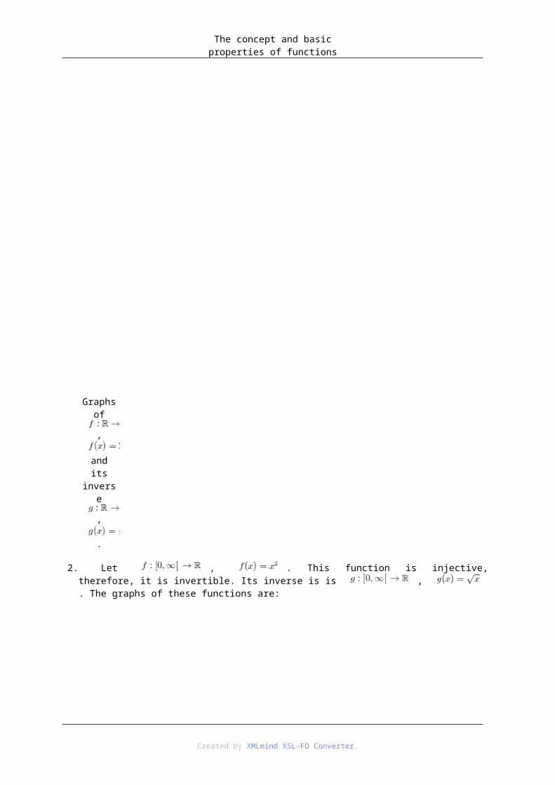
2. Let , . This function is injective, therefore, it is invertible. Its inverse is is , . The graphs of these functions are:
Created by XMLmind XSL-FO Converter.

The concept and basic properties of functions
Graphs of
,
and its inverse
,
.
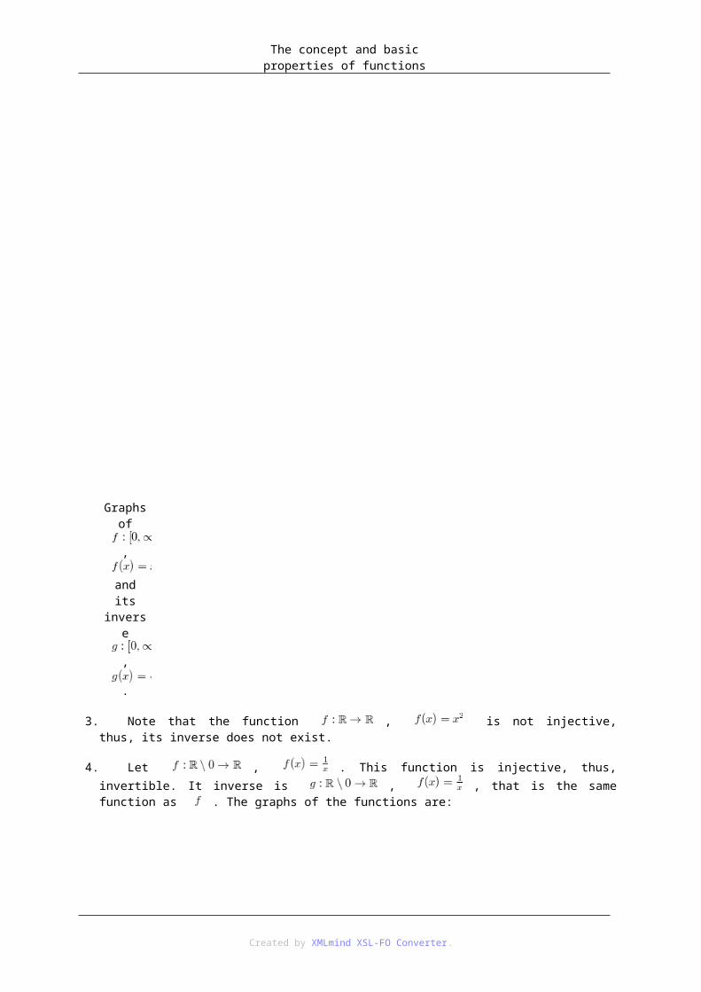
3. Note that the function , is not injective, thus, its inverse does not exist.
4. Let , . This function is injective, thus, invertible. It inverse is , , that is the same function as . The graphs of the functions are:
Created by XMLmind XSL-FO Converter.
The concept and basic properties of functions
Graphs of
,
and its inverse
,
.
Exercise 1.9. Illustrate the following functions with a diagram, investigate if they are invertible or not and, in the case when they exist, determine their inverse functions and draw their diagrams:
a) , ,
, , , , , ;
b) Let , ,
, , , , ;
c) , ,
, , , , ;
d) , ,
, , , , , .
Created by XMLmind XSL-FO Converter.
The concept and basic properties of functions
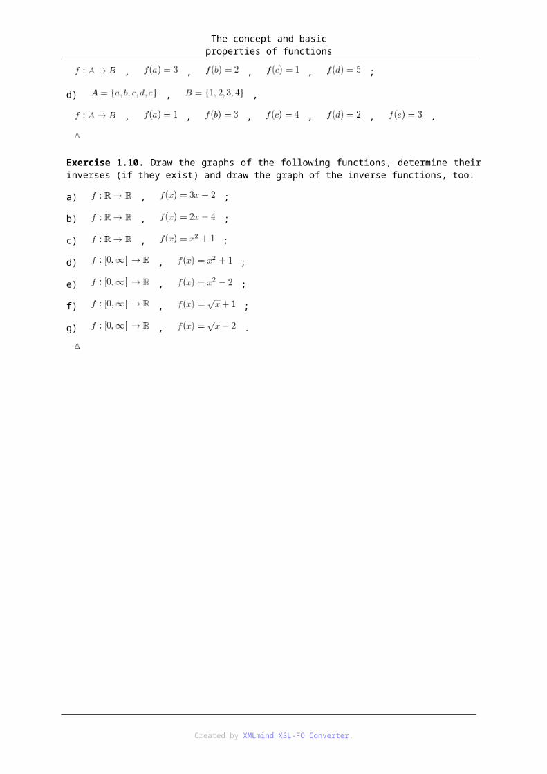
Exercise 1.10. Draw the graphs of the following functions, determine their inverses (if they exist) and draw the graph of the inverse functions, too:
a) , ;
b) , ;
c) , ;
d) , ;
e) , ;
f) , ;
g) , .
Created by XMLmind XSL-FO Converter.

Chapter 2. Types of functions1. 2.1. Linear functionsDefinition 2.1. A function of the form
is called a linear function.
Remark. We remind the student that for all pairs of points and lying on the same (not vertical) straight line in the plane (represented in a Cartesian coordinate system) the quantity
is constant (i.e. it is independent of the choice of and ). This number is called the slope of the line.
Theorem 2.2. Let be a linear function with .
1. The graph of is a straight line. More precisely, the graph of is the line with equation . Further, the graph of is a horizontal line if and only if .
2. The -intercept of the graph of is the point .
3. Whenever the only -intercept of the graph of is the point . If then the graph of has no -intercept. If then the graph of
is the -axis itself.
The above theorem suggests the definition below:
Definition 2.3. The number is called the slope of the linear function .
Theorem 2.4. Fix a Cartesian coordinate system in the two dimensional plane. Except for the vertical lines every straight line in the plane is the graph of a linear function. The function corresponding to a line may be given by the following formulas:
1. The slope-intercept formula
2. The point-slope formula
Created by XMLmind XSL-FO Converter.
Types of functions
3. The point-point formula
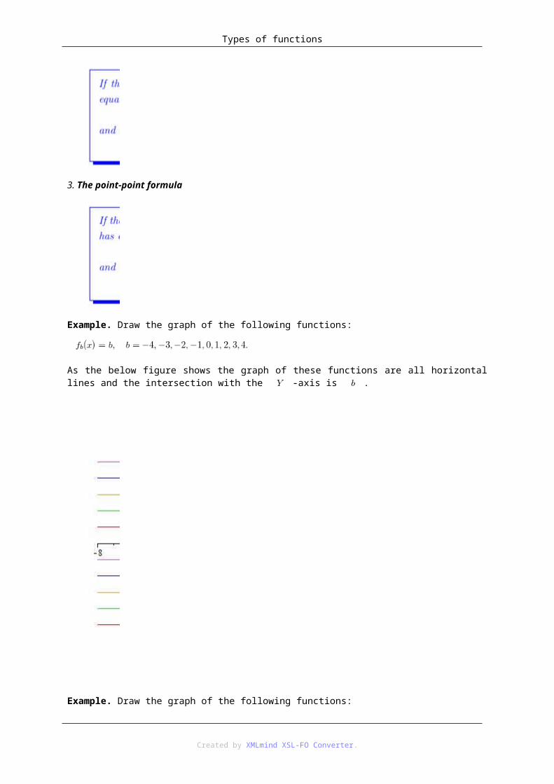
Example. Draw the graph of the following functions:
As the below figure shows the graph of these functions are all horizontal lines and the intersection with the -axis is .
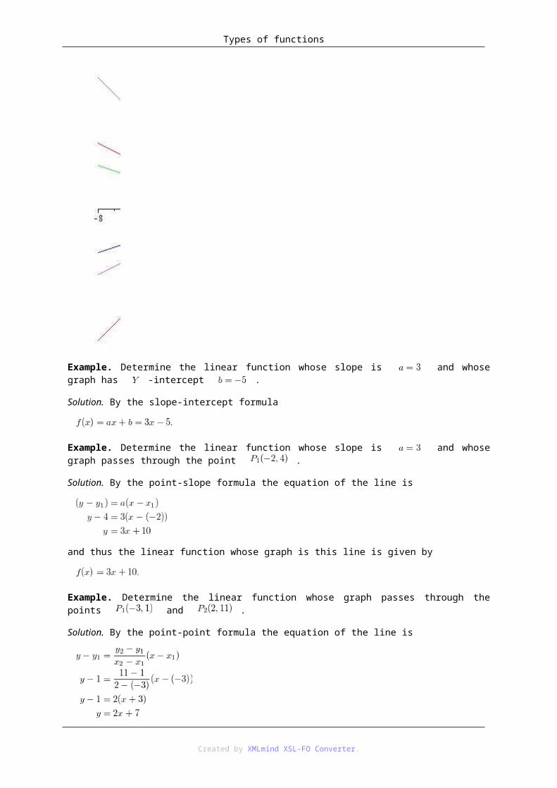
Example. Draw the graph of the following functions:
As the below figure shows the graph of these functions are parallel to each other and the intersection with the -axis is .
Created by XMLmind XSL-FO Converter.

Types of functions
Example. Draw the graph of the following functions:
As the below figure shows the graph of each of these functions goes through the origin, and if is positive, then the line passes through the 1st and 3rd quadrant, if is negative, then it passes through the 2nd and 4th quadrant. In the case of the graph is the -axis
Created by XMLmind XSL-FO Converter.
Types of functions
Example. Determine the linear function whose slope is and whose graph has -intercept .
Solution. By the slope-intercept formula
Example. Determine the linear function whose slope is and whose graph passes through the point .
Solution. By the point-slope formula the equation of the line is
and thus the linear function whose graph is this line is given by
Example. Determine the linear function whose graph passes through the points and .
Solution. By the point-point formula the equation of the line is
Created by XMLmind XSL-FO Converter.

Types of functions
and thus the linear function whose graph is this line is given by
Exercise 2.1. Determine the linear function whose slope is and whose graph has -intercept where:
Sketch the graph of these functions.
Exercise 2.2. Determine the linear function whose slope is and whose graph passes through the point .
Exercise 2.3. Determine the linear function whose graph passes through the points and
2. 2.2. Quadratic functionsDefinition 2.5. A function defined by
is called a quadratic function. If the quadratic function is given by a formula of the above shape, we say that it is given in general form.
Theorem 2.6. (The canonical form of a quadratic function)
Created by XMLmind XSL-FO Converter.
Types of functions
Let be a quadratic function with , . Put . Then can be written in the form
with and .
Proof.
Example. Compute the canonical form of the following quadratic function:
Solution.
Another solution to the problem is to use directly Theorem 2.6 [60]. We have , and
thus and , and we get
Theorem 2.7. (The factorized form of a quadratic function)
Let be a quadratic function with , . Put and if then put
Then can be written in the form
If then and the above factorization takes the form .
Theorem 2.8. Let be a quadratic function with , . Put and if then put
Created by XMLmind XSL-FO Converter.

Types of functions
The graph of is a parabola with the following properties:
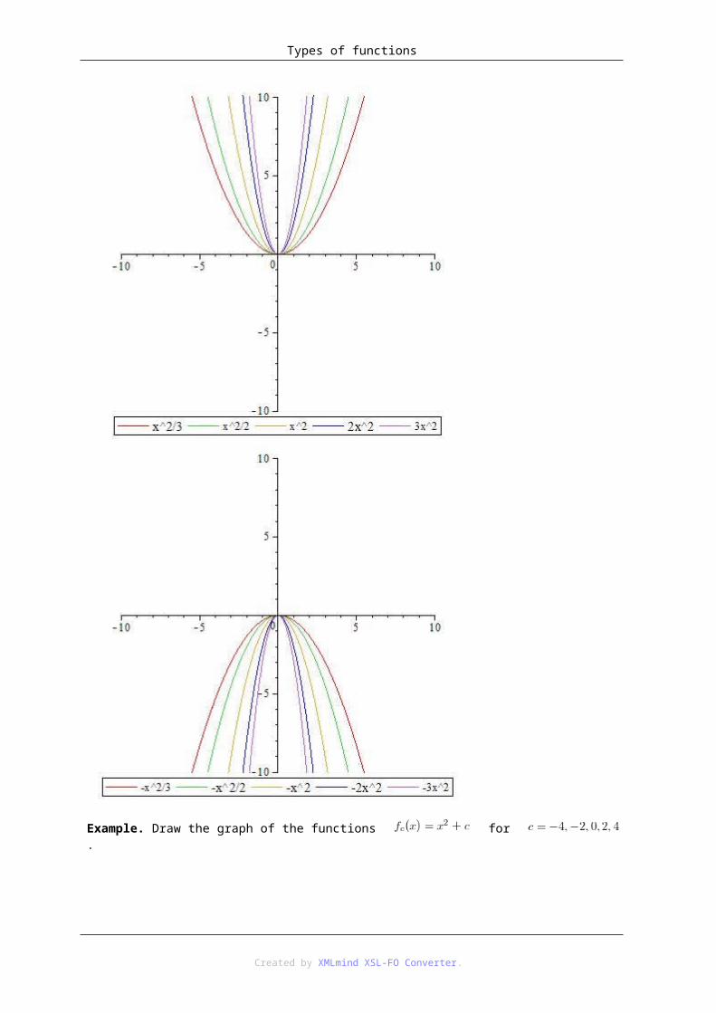
Example. Draw the graph of the functions for and for .
Created by XMLmind XSL-FO Converter.

Types of functions
Example. Draw the graph of the functions for .
Example. Draw the graph of the functions for .
Created by XMLmind XSL-FO Converter.

Types of functions
Example. Draw the graph of the functions for .
Exercise 2.4. Let be the quadratic function below.
1. Give the canonical form.
Created by XMLmind XSL-FO Converter.
Types of functions
2. If give the factorized form.
3. Give the -intercept and -intercepts of the graph of .
4. Give the vertex of the graph of .
5. Draw the graph of .
3. 2.3. Polynomial functions3.1. 2.3.1. Definition of polynomial functionsDefinition 2.9. A function given by
with and given is called a polynomial function.
Remark. Linear and quadratic functions are special polynomial functions.
3.2. 2.3.2. Euclidean division of polynomials in one variableIn this section we present the division algorithm for univariate polynomials with complex, real or rational coefficients. This procedure is a straightforward generalization of the long division of integers.
Created by XMLmind XSL-FO Converter.
Types of functions
Example. Divide the polynomial by .
Remark. If in the dividend polynomial there are missing terms of lower degrees, than it is wise to include them with coefficient in the scheme, so that for their like terms there is place below them.
Example. Divide the polynomial by .
Exercise 2.5. Divide the polynomial by the polynomial using the procedure of Euclidean division:
Created by XMLmind XSL-FO Converter.

Types of functions
3.3. 2.3.3. Computing the value of a polynomial functionTo compute the value of a polynomial function at it is clearly possible by the general method, i.e. by replacing each the variable at each occurrence of it by , and computing the value of the resulting expression. However in this case there is a better way to compute it, by using the following Theorem:
Theorem 2.10. (Horner's scheme) Let with , and with be two polynomials. Build the following table:
where
Then the quotient of the polynomial division of by is the polynomial
and the remainder is the constant polynomial . Further, we also have
Remark. In other words the above theorem states that in Horner's scheme the numbers in the first line are the coefficients of the polynomial , and the numbers computed in the second line of the scheme are the following:
• the first number is the zero of the polynomial
• the next numbers (except for the last one) are the coefficients of the quotient polynomial of the polynomial
Created by XMLmind XSL-FO Converter.

Types of functions
division of by
• the last number is the remainder of the above division, but it is also the value of the polynomial at .
Example. Now we compute the value of the polynomial function in using Horner's scheme. The first place in the first line is empty, then we list the coefficients of .
The first element in the second line of the Horner's scheme will be . Then we compute the consecutive elements of the second line using 2.3 to get
This means that .
Remark. If in the dividend polynomial there are missing terms of lower degrees, than it is compulsory to include the coefficients of these terms (i.e. -s) in the upper row of the Horner's scheme.
Example. We compute the value of the polynomial function at using Horner's scheme. The first place in the first row is empty, then we list the coefficients of , including the coefficient of . The first element in the second row of the Horner's scheme will be . Then we compute the consecutive elements of the second line using 2.3 to get
This means that .
Exercise 2.6. Compute the value of the following polynomial function at the given value of the indeterminate :
Created by XMLmind XSL-FO Converter.

Types of functions
4. 2.4. Power functionsDefinition 2.11. A function given by
with given and is called a power function.
Example. Draw the graph of the functions , for and for .
Created by XMLmind XSL-FO Converter.

Types of functions
5. 2.5. Exponential functionsDefinition 2.12. A function given by
Created by XMLmind XSL-FO Converter.

Types of functions
with a given , is called an exponential function.
Example. Draw the graph of the functions , for and for.
Definition 2.13. In the sequel we denote by the Euler constant
Definition 2.14. The function given by
is called the natural exponential function.
Example. Draw the graph of the functions .
Created by XMLmind XSL-FO Converter.

Types of functions
Example. Draw the graph of the functions .
6. 2.6. Logarithmic functions
Created by XMLmind XSL-FO Converter.
Types of functions
Definition 2.15. A function given by
with a given , is called a logarithmic function.
Example. Draw the graph of the functions , for and for.
Definition 2.16. Recall that denotes the Euler constant
Definition 2.17. The function given by
where is the Euler-constant is called the natural logarithmic function. We denote the logarithm on base by , and similarly the natural logarithmic function by .
Remark. The natural logarithmic function is sometimes also denoted by .
Example. Draw the graph of the functions , and , .
Created by XMLmind XSL-FO Converter.
Types of functions
Remark. We also recall that the logarithmic function on base is denoted by .
Created by XMLmind XSL-FO Converter.

Chapter 3. Trigonometric functions1. 3.1. Measures for angles: Degrees and RadiansIn geometry an angle is considered to be a figure which consists of two half-lines called the sides, sharing a common endpoint, called the vertex. So basically we have the following kinds of angles:
By considering also the points of the plane between the two sides as parts of the angle, we may extend the notion of angle to reflex angles (those larger than a straight angle) and full angles:
Definition 3.1. Divide the full angle into equal angles. The measure for one such part is defined to be one degree, and the measure of any angle will be as many degrees as many parts of 1 degree fit between the sides of the angle. The notation for degree is a circle "in the exponent" e.g. .
What is the reason for choosing the number ? In one hand, is divisible by many integers. So the half, the third, the quoter, the one fifth, one sixth, one eighth, one tenth, one twelfth of a whole circle has an integer measure, and this is very convenient. On the other hand is close to the number of days in the astronomical years, which was convenient in astronomy. In geometry this measure for angles is also convenient, however, in trigonometry and analysis it is inconvenient, and there we use radians to measure the angles:
Definition 3.2. The measure of an angle in radians is the length of the arc corresponding to the angle (as a central angle) of a unit circle. This means that the measure of a full angle is . When measuring angles in radians the size of the angle is a pure number without explicitly expressed unit.
Remark. In many cases the word "angle" will be used not only for the geometric figure, but also for its measure.
Theorem 3.3. Let us have an angle of measure . Then its measure in radians is .
Created by XMLmind XSL-FO Converter.

Trigonometric functions
Let us have an angle of measure radians. Then its measure in degrees is .
Example. The measure of the most important angles in degrees and radians:
2. 3.2. Rotation anglesTo extend the notion of angles such that every real number corresponds to the measure of an angle we do the following:
Remark. If is measured in degrees on the picture below, then the radius which corresponds to the angle is the same which corresponds to for any .
Created by XMLmind XSL-FO Converter.

Trigonometric functions
Definition 3.4. Angles which have the same terminal side are called coterminal. Further, we say that an angle is on the first circle if its measure in degrees is on the interval (or alternatively, if its measure in radians is in the interval ).
Theorem 3.5. Every rotation angle is coterminal with an angle on the first circle.
The two coordinate axes divide the plane into four quadrants, as it is shown on the figure below.
We say that an angle belongs to one of the quadrants, if its terminal side is in that quadrant.
3. 3.3. Definition of trigonometric functions for acute angles of right triangles3.1. 3.3.1. The basic definitions
Created by XMLmind XSL-FO Converter.

Trigonometric functions
The definitions above may also be formulated in the following way
Definition 3.6. Let be one acute angle of a right triangle.
• The sine of is defined by
• The cosine of is defined by
• The tangent of is defined by
• The cotangent of is defined by
Remark. The definition of trigonometric functions above are independent of the choice of the triangle. Indeed, if we have two right triangles having an acute angle of measure , then these triangles are similar to each other. Thus the quotient of the length of the two corresponding sides in the two triangles is the same.
Example. Let the lengths of the sides of a right triangle be . Let be the angle opposite to the leg of length . Compute , , , .
Solution.
Created by XMLmind XSL-FO Converter.

Trigonometric functions
3.2. 3.3.2. Basic formulas for trigonometric functions defined for acute anglesTheorem 3.7. (The cofunction identities) Let be an acute angle in a right triangle. Then we have:
Theorem 3.8. (The quotient identities) Let be an acute angle in a right triangle. Then we have:
Theorem 3.9. (The trigonometric theorem of Pythagoras in right triangles) Let be an acute angle in a right triangle. Then we have:
Proof of Theorems 3.7 [79], 3.8 [79], 3.9 [79]Let be a right triangle, the right angle being at the vertex and with the size of the angle at vertex being .
Created by XMLmind XSL-FO Converter.
Trigonometric functions
Finally, we prove Theorem 3.9 [79]. The Theorem of Pythagoras for the triangle states that . Using this we get
which conclude the proof of Theorem 3.9 [79].
3.3. 3.3.3. Trigonometric functions of special anglesIn applications the angles are of special interest. In this paragraph we compute the trigonometric functions of these angles.
Theorem 3.10. The values of the trigonometric functions of are summarized in the following table.
Proof. To prove the statements of the theorem concerning the angles and we consider an equilateral triangle , and we draw its bisector .
Created by XMLmind XSL-FO Converter.

Trigonometric functions
In this triangle the Theorem of Pythagoras gives:
so we get
Clearly, have , and since is the bisector of the angle we also have . Thus, in the right triangle we have
and similarly,
Created by XMLmind XSL-FO Converter.

Trigonometric functions
Clearly, we also have , so from the triangle using its angle we get:
This concludes the proof of our theorem.
4. 3.4. Definition of the trigonometric functions over
Definition 3.11. Consider a unit circle with a rotating radius. Let be a rotation angle on this circle. Let the intersection point of the line of the terminal side of by the tangent line drawn to the circle in the point
, if it exists at all, be denoted by . Similarly, let the intersection point of the line of the terminal side of by the tangent line drawn to the circle in the point , if it exists at all, be denoted by
. We remind that the point does not exist if for , and does not exist if for .
Created by XMLmind XSL-FO Converter.

Trigonometric functions
Then for any we define the trigonometric functions of as follows:
Remark. For acute angles Definition 3.11 [82] coincides with the definition of trigonometric functions in right triangles. Thus, Definition 3.11 [82] extends the former concept of , , and for any real number. More precisely,
• and are defined for any real number ;
• is not defined for for , but it is defined for every other ;
• is not defined for for , but it is defined for every other .
5. 3.5. The period of trigonometric functionsTheorem 3.12. The trigonometric functions sine, cosine, tangent and cotangent are periodic. Further, for the period of these functions we have:
Created by XMLmind XSL-FO Converter.

Trigonometric functions
Proof. If we investigate the figure in Definition 3.11 [82] we see that for any angle the terminal side of and is the same, so for and the point will be the same, which
proves that and . Further, it is clear that is the smallest angle with this property holding for every . This proves statements 1) and 2) of Theorem 3.12 [83].
Next, we also see that the terminal side of and the terminal side of are on the same line, thus fixing the same points and , which proves and . Further, it is clear again, that is the smallest angle with this property holding for every . This proves statements 3) and 4) of Theorem 3.12 [83].
Corollary 3.13. Theorem 3.12 [83] proves that we have
6. 3.6. Symmetry properties of trigonometric functionsTheorem 3.14. The functions are odd functions, and the function is an even function. This means that we have the following formulas:
Created by XMLmind XSL-FO Converter.

Trigonometric functions
7. 3.7. The sign of trigonometric functionsThe sign of the trigonometric functions , , , is determined by the situation of the terminal side of . Whenever belongs to one of the four quadrants the sign of the above functions is already determined, and the same is true for the cases when the terminal side of is at border of two quadrants.
We may summarize the information about the sign of the trigonometric functions , , , as follows:
1. If is in the quadrant then
2. If is at the border of the and quadrant, i.e. then
3. If is in the quadrant then
4. If is at the border of the and quadrant, i.e. then
Created by XMLmind XSL-FO Converter.

Trigonometric functions
5. If is in the quadrant then
6. If is at the border of the and quadrant, i.e. then
7. If is in the quadrant then
8. If is at the border of the and quadrant, i.e. then
Created by XMLmind XSL-FO Converter.

Trigonometric functions
Remark. The sign of trigonometric functions can also be summarized by the following diagrams:
8. 3.8. The reference angleDefinition 3.15. Let be a rotation angle such that its terminal side is not on the coordinate axis. The acute angle formed by the -axis and the terminal side of is called the reference angle of .
Theorem 3.16. Let be a rotation angle, and let be its reference angle. Then we have the following:
Theorem 3.17. Let be a rotation angle, and let be its reference angle. The we have the following:
• If is in the first quadrant then ;
• If is in the second quadrant then ;
• If is in the third quadrant then ;
• If is in the fourth quadrant then .
Remark. The above theorem can be summarized by the below diagram:
Created by XMLmind XSL-FO Converter.

Trigonometric functions
The theorem below is a variant of Theorem 3.16 [87]:
Theorem 3.18. Let be a rotation and be its reference angle. Let be the sign function on , i.e.
Then we have the following
Example. Compute the exact value of the following expressions:
1.
2.
3.
Solution.
1. We shall use Theorem 3.18 [88]. First we mention that is in the third quadrant, so and by Theorem 3.17 [87] the reference angle of is . So we have
2. Since is in the fourth quadrant we have
Created by XMLmind XSL-FO Converter.

Trigonometric functions
3. Since is in the fourth quadrant we have
Example. Compute the exact value of the following expressions:
1.
2.
3.
Solution.
1. In contrast to the previous example the angle is not on the first circle, so we cannot use Theorem 3.17 [87] directly to compute the reference angle of . First we have to compute the angle on the first circle which corresponds to (i.e. has the same terminal side as ). This means that we have to subtract form as many times as it is needed the result to be on the first circle. So we have
Now like in the previous exercise we shall use Theorem 3.18 [88]. Since is in the fourth quadrant we have
2. Similarly to the previous example we have
3. Finally we use the same method to solve the last exercise:
We mention that instead of finding the angle on the first circle with the same terminal side as we also can subtract from as many times that the result is between and . This is since the period of is .
The same applies for , however it is important that this latter is not true in the case of and , since their period is . This means that in the case of and we have to
subtract an integer multiple of and it is not possible to replace by .
Created by XMLmind XSL-FO Converter.

Trigonometric functions
Exercise 3.1. Compute the exact value of the following expressions:
9. 3.9. Basic formulas for trigonometric functions defined for arbitrary anglesThe formulas presented in Section 3.3.2 generalize automatically for trigonometric functions defined for arbitrary angles.
9.1. 3.9.1. Cofunction formulasTheorem 3.19. Let be a rotation angle for which the trigonometric functions in the below formulas are defined. Then we have the following formulas which connect trigonometric functions of to cofunctions of
:
9.2. 3.9.2. Quotient identitiesTheorem 3.20. Let be a rotation angle for which the trigonometric functions in the below formulas are defined. Then we have:
Created by XMLmind XSL-FO Converter.

Trigonometric functions
9.3. 3.9.3. The trigonometric theorem of PythagorasTheorem 3.21. Let be a rotation angle. Then we have:
10. 3.10. Trigonometric functions of special rotation anglesPreviously, we computed the values of the trigonometric functions for the acute angles , which are of special interest for applications. In this paragraph we extend this for rotation angles with their reference angles being :
Theorem 3.22. The values of the trigonometric functions of some important angles are summarized in the following table.
where the sign ` ' means that the corresponding value is not defined.
11. 3.11. The graph of trigonometric functions11.1. 3.11.1. The graph of
Created by XMLmind XSL-FO Converter.

Trigonometric functions
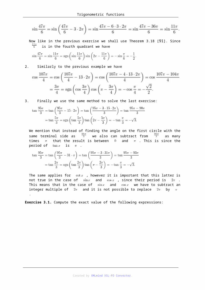
11.2. 3.11.2. The graph of
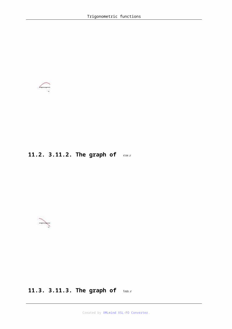
11.3. 3.11.3. The graph of
Created by XMLmind XSL-FO Converter.
Trigonometric functions
11.4. 3.11.4. The graph of
Created by XMLmind XSL-FO Converter.

Trigonometric functions
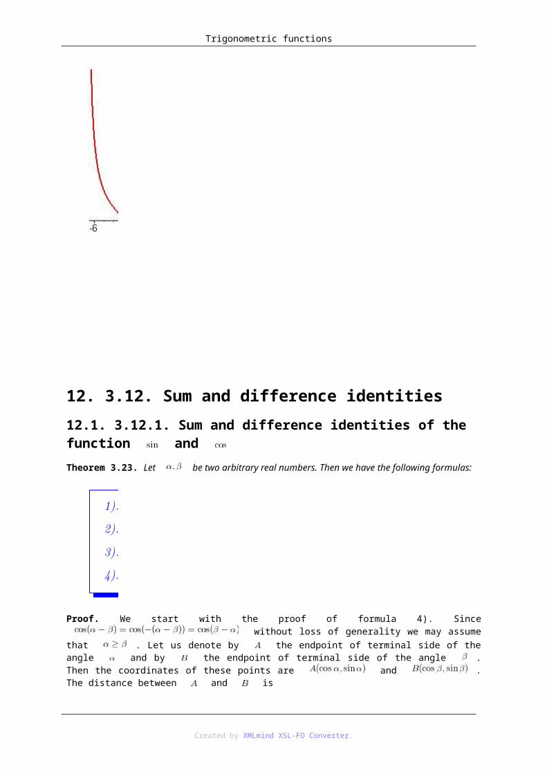
12. 3.12. Sum and difference identities12.1. 3.12.1. Sum and difference identities of the function and Theorem 3.23. Let be two arbitrary real numbers. Then we have the following formulas:
Proof. We start with the proof of formula 4). Since without loss of generality we may assume that . Let us denote by the endpoint of terminal side of the angle and by the endpoint of terminal side of the angle . Then the coordinates of these points are and . The distance between and is
Created by XMLmind XSL-FO Converter.

Trigonometric functions
Further, the size of the angle is just , and if we rotate this angle in such a way that the side is moved to the -axis (i.e. the image of lies on the -axis), then the side is moved to such that is just the terminal side of the rotation angle . So we
have
Further, by the isometric property of the rotations we have , which gives
Now rising to the square both sides, subtracting from both sides and dividing them by we get the required identity
Now the proof of the third identity is straightforward:
The proof of the first identity is
Finally, the proof of the second identity is
Example. Compute and .
Solution. We do not know the values of the exact value of the trigonometric functions of from tables, since is not an "important" angle, however since
and we know the exact values of the trigonometric functions on and from our tables, we are able to compute and using Theorem 3.23 [94]:
Created by XMLmind XSL-FO Converter.
Trigonometric functions
and
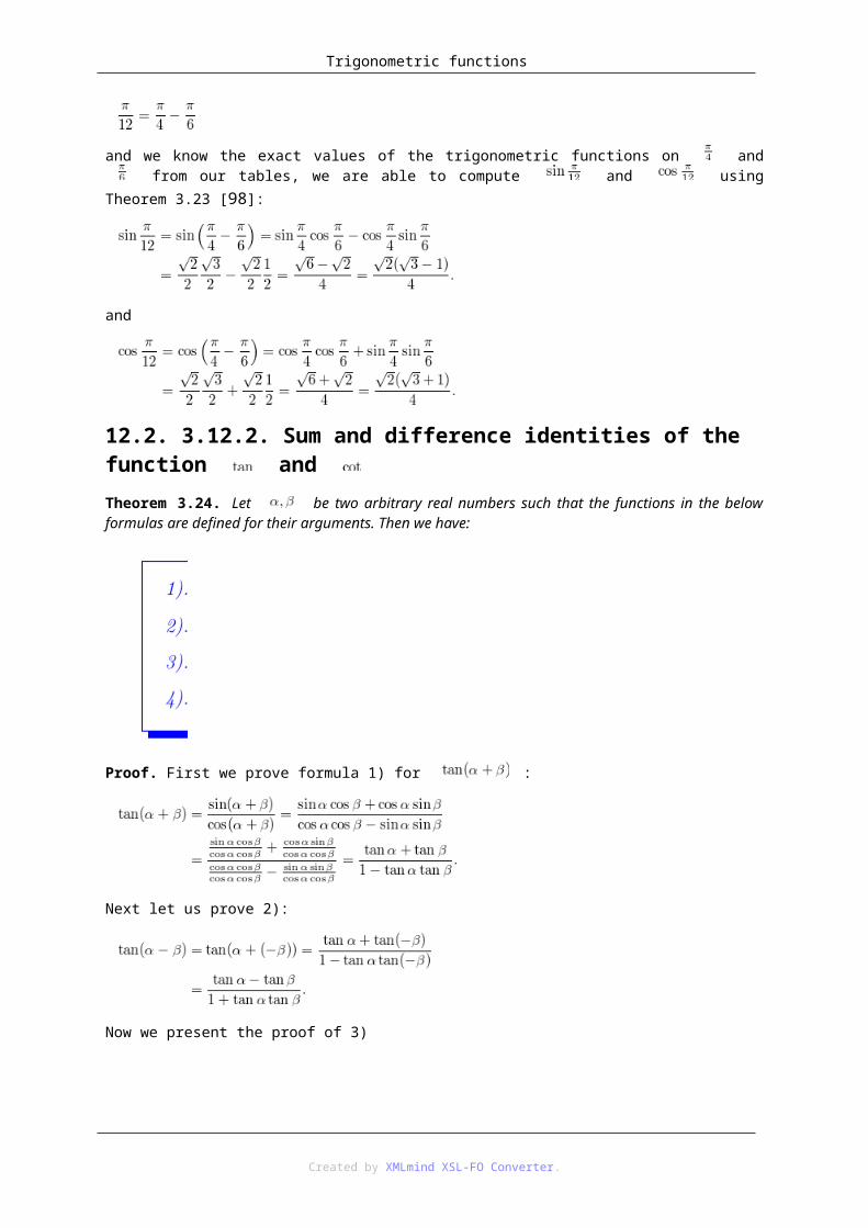
12.2. 3.12.2. Sum and difference identities of the function and Theorem 3.24. Let be two arbitrary real numbers such that the functions in the below formulas are defined for their arguments. Then we have:
Proof. First we prove formula 1) for :
Next let us prove 2):
Now we present the proof of 3)
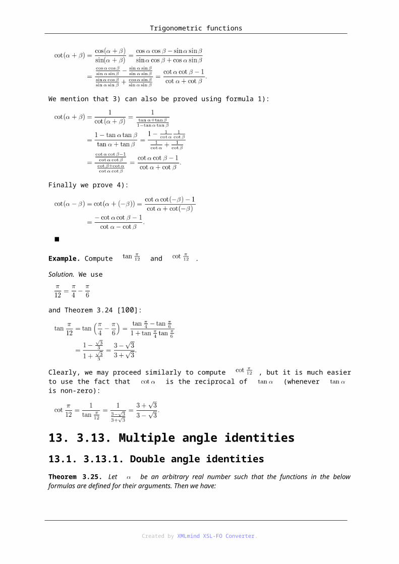
We mention that 3) can also be proved using formula 1):
Created by XMLmind XSL-FO Converter.

Trigonometric functions
Finally we prove 4):
Example. Compute and .
Solution. We use
and Theorem 3.24 [96]:
Clearly, we may proceed similarly to compute , but it is much easier to use the fact that is the reciprocal of (whenever is non-zero):
13. 3.13. Multiple angle identities13.1. 3.13.1. Double angle identitiesTheorem 3.25. Let be an arbitrary real number such that the functions in the below formulas are defined for their arguments. Then we have:
Proof. For proving this theorem we use the corresponding formulas from Theorem 3.23 [94] and Theorem 3.24
Created by XMLmind XSL-FO Converter.
Trigonometric functions
[96]. First we prove formula 1):
Now we prove 2):
For proving the other two statements of formula 2) we also need to use the trigonometric theorem of Pythagora, i.e. the formula
So we get
Now we prove formulas 3) and 4)
Example. Compute and .
Solution. Recall that we already have computed and in Section 3.12.1, using and Theorem 3.23 [94], and we got the result:
Now we wish to use identity 2) of Theorem 3.25 [97] to compute and . Indeed, we have
Expressing from this expression we get
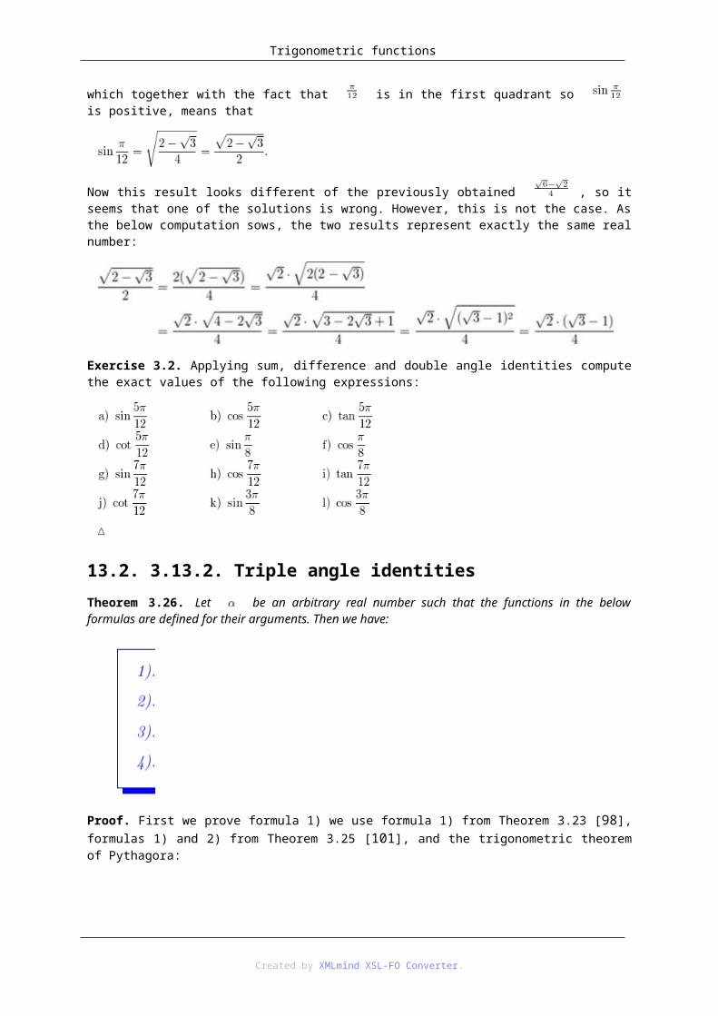
which together with the fact that is in the first quadrant so is positive, means that
Now this result looks different of the previously obtained , so it seems that one of the solutions is wrong. However, this is not the case. As the below computation sows, the two results represent exactly the same real number:
Created by XMLmind XSL-FO Converter.

Trigonometric functions
Exercise 3.2. Applying sum, difference and double angle identities compute the exact values of the following expressions:
13.2. 3.13.2. Triple angle identitiesTheorem 3.26. Let be an arbitrary real number such that the functions in the below formulas are defined for their arguments. Then we have:
Proof. First we prove formula 1) we use formula 1) from Theorem 3.23 [94], formulas 1) and 2) from Theorem 3.25 [97], and the trigonometric theorem of Pythagora:
Similarly, to prove formula 1) we need formula 3) from Theorem 3.23 [94], formulas 1) and 2) from Theorem 3.25 [97], and the trigonometric theorem of Pythagora:
Now we prove formula 3) using formula 1) of Theorem 3.24 [96] and formula 3) of Theorem 3.25 [97]:
Created by XMLmind XSL-FO Converter.
Trigonometric functions
Finally, we prove formula 4) by using formula 3) of Theorem 3.24 [96] and formula 4) of Theorem 3.25 [97]:
14. 3.14. Half-angle identitiesTheorem 3.27. Let be an arbitrary real number such that the functions in the below formulas are defined for their arguments. Then we have:
Proof. To prove the half-angle formulas we basically use identity 2) of Theorem 3.25 [97], which applied for instead of gives
Expressing from the above equation we get
meanwhile expressing leads to the identity
These conclude the proof of identities 1) and 2). By dividing the two latter identities we just get 3) and 4). So it remains to prove 5) and 6). To do so first we mention that by the trigonometric theorem of Pythagoras we have
, which means that , and thus we have
Thus, whenever , we get
Created by XMLmind XSL-FO Converter.
Trigonometric functions
and
However, we mention that, by , whenever and is defined we have . So the second equality of both 5) and 6) is proved.
To conclude the proof of this theorem we write
and
This concludes the proof of the theorem.
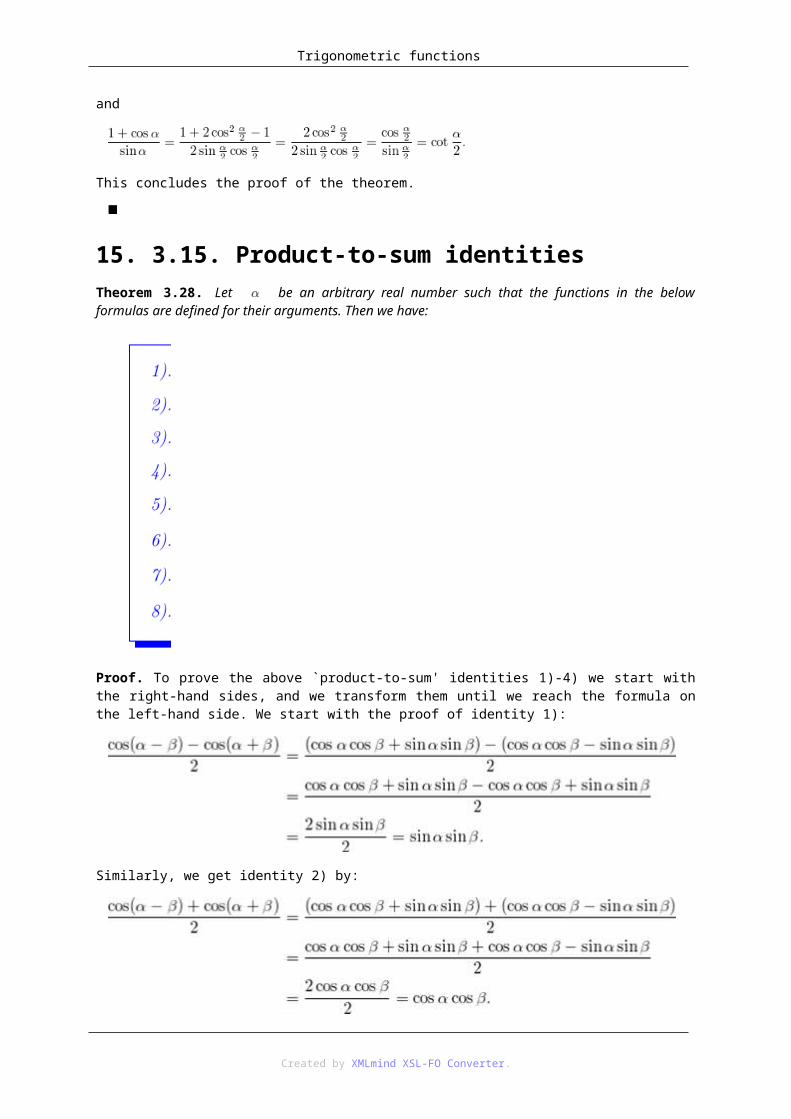
15. 3.15. Product-to-sum identitiesTheorem 3.28. Let be an arbitrary real number such that the functions in the below formulas are defined for their arguments. Then we have:
Proof. To prove the above `product-to-sum' identities 1)-4) we start with the right-hand sides, and we transform them until we reach the formula on the left-hand side. We start with the proof of identity 1):
Created by XMLmind XSL-FO Converter.

Trigonometric functions
Similarly, we get identity 2) by:
The proof of identity 3) is
and for the proof of identity 4) we have
For the proof of identities 5)–8) we have to divide correspondingly two of the identities 1)–4). So we have
16. 3.16. Sum-to-product identitiesTheorem 3.29. Let be an arbitrary real number such that the functions in the below formulas are defined for their arguments. Then we have:
Created by XMLmind XSL-FO Converter.
Trigonometric functions
Proof. Again we shall start from the right-hand side and we will do equivalent transformations of the expressions until we reach the left-hand side of the corresponding formula. We start with identity 1):
Similarly, we prove identity 2):
The proof of identity 3) is the following:
Finally, the proof of identity 4) is:
Created by XMLmind XSL-FO Converter.

Trigonometric functions
Created by XMLmind XSL-FO Converter.

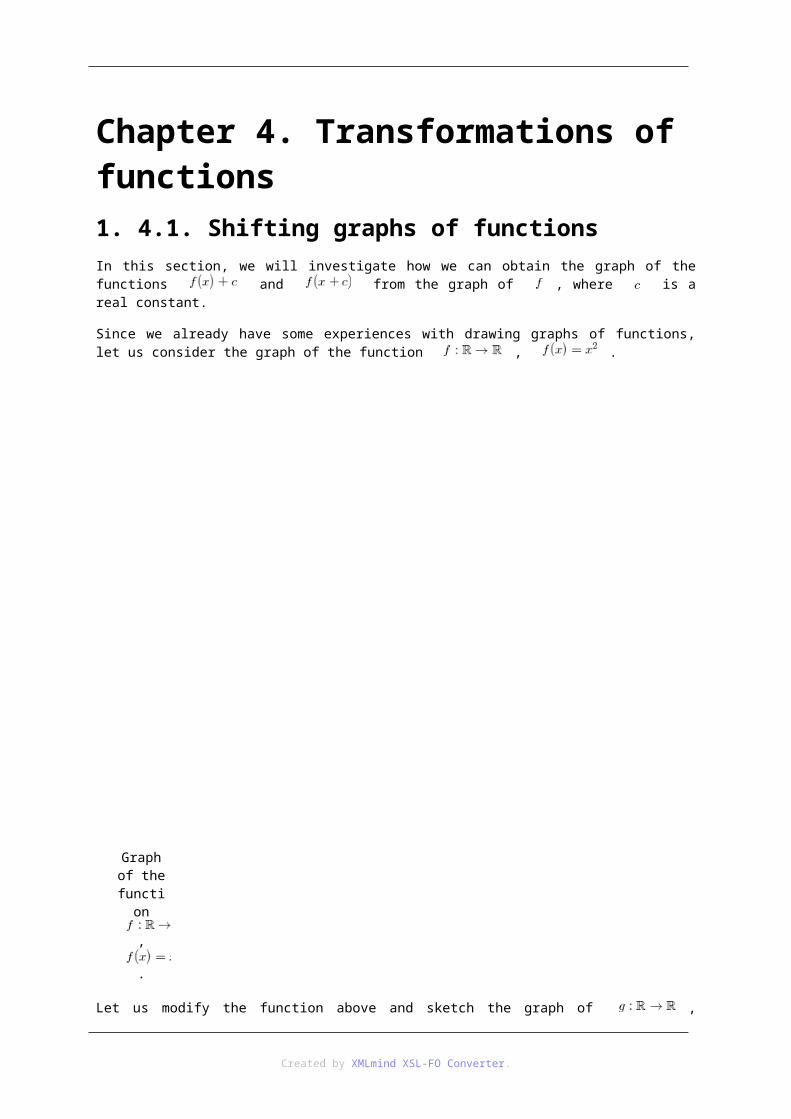
Chapter 4. Transformations of functions1. 4.1. Shifting graphs of functionsIn this section, we will investigate how we can obtain the graph of the functions and from the graph of , where is a real constant.
Since we already have some experiences with drawing graphs of functions, let us consider the graph of the function , .
Graph of the
function
,
.
Let us modify the function above and sketch the graph of , now.
Created by XMLmind XSL-FO Converter.
Transformations of functions
Graph of the
function
,
.
Drawing both graphs above in the same coordinate system, we obtain the following:
Created by XMLmind XSL-FO Converter.

Transformations of functions
Graphs of the
functions
,
and
,
.
It is easy to see, that, starting with a point of the graph of the function , we can obtain the element of the graph of by . Since this property is valid for all pairs of points
and of the graphs of our functions, we may obtain the graph of if we shift (or move, or translate) the graph of upwards by units. Obviously, this method works for all positive integers
. It is also clear, that, in the case when is a negative real number, we have to shift (or move, or translate) the graph of downwards by units (where denotes the absolute value of ). Finally, it is trivial, that, if then the functions and coincide.
Let us sketch now the graph of the function , .
Created by XMLmind XSL-FO Converter.
Transformations of functions
Graph of the
function
,
.
We shall illustrate the graphs of and in the same coordinate system now.
Created by XMLmind XSL-FO Converter.

Transformations of functions
Graphs of the
functions
,
and
,
.
Similarly to the case above, we can see, that we may obtain the graph of if we shift (or move, or translate) the graph of to the left by units. This method also works for each positive integer . Furthermore, if is a negative real number, we have to shift (or move, or translate) the graph of to the right by units. (Here, it is also true that, in the case when then the functions and
are equal.)
It is easy to see that the argumentation above is independent from the concrete functions , and , it only depends on the connection between the functions. Thus, we can give a general method for the types of function transformations considered above. In order describe this method, let us denote by the translation of the set by units. More precisely, if is a set and is a real number,
denotes the set .
Let be a real number, be a set and let us consider a function .
– In the case when is nonnegative, we can obtain the graph of the function , by shifting (or moving) the graph of the function by units upwards.
– In the case when is negative, we can obtain the graph of the function ,
Created by XMLmind XSL-FO Converter.
Transformations of functions
by shifting (or moving) the graph of the function by units downwards.
– In the case when is nonnegative, we can obtain the graph of the function , by shifting (or moving) the graph of the function by units to the left.
– In the case when is negative, we can obtain the graph of the function , by shifting (or moving) the graph of the function by units to the right.
Examples.
1. Let us sketch the graph of the function , using the graph of , .
Graph of the
function
,
.
Created by XMLmind XSL-FO Converter.

Transformations of functions
Graphs of the
functions
,
and
,
.
2. Let us sketch the graph of the function , using the graph of , .
Created by XMLmind XSL-FO Converter.

Transformations of functions
Graphs of the
functions
,
and
,
.
3. Let us sketch the graph of the function , using the graph of , .
Created by XMLmind XSL-FO Converter.
Transformations of functions
Graph of the
function
,
.
Created by XMLmind XSL-FO Converter.
Transformations of functions
Graphs of the
functions
,
and
,
.
4. Let us sketch the graph of the function , using the graph of , .
Created by XMLmind XSL-FO Converter.

Transformations of functions
Graphs of the
functions
,
and
,
.
5. Let us sketch the graphs of the function , using the graph of , .
Created by XMLmind XSL-FO Converter.

Transformations of functions
Graph of the
function
,
.
Created by XMLmind XSL-FO Converter.

Transformations of functions
Graphs of the
functions
,
and
,
.
6. Let us sketch the graphs of the function , using the graph of , .
Created by XMLmind XSL-FO Converter.
Transformations of functions
Graphs of the
functions
,
and
,
.
7. Let us sketch the graphs of the function , using , .
Created by XMLmind XSL-FO Converter.

Transformations of functions
Graph of the
function
,
.
Created by XMLmind XSL-FO Converter.

Transformations of functions
Graphs of the
functions
,
and
,
.
8. Let us sketch the graphs of the function , using , .
Created by XMLmind XSL-FO Converter.

Transformations of functions
Graphs of the
functions
,
and
,
.
9. Let us sketch the graph of the function , using the graph of , .
Created by XMLmind XSL-FO Converter.
Transformations of functions
Graph of the
function
,
.
Created by XMLmind XSL-FO Converter.
Transformations of functions
Graphs of the
functions
,
and
,
.
10. Let us sketch the graph of the function , using the graph of , .
Created by XMLmind XSL-FO Converter.

Transformations of functions
Graphs of the
functions
,
and
,
.
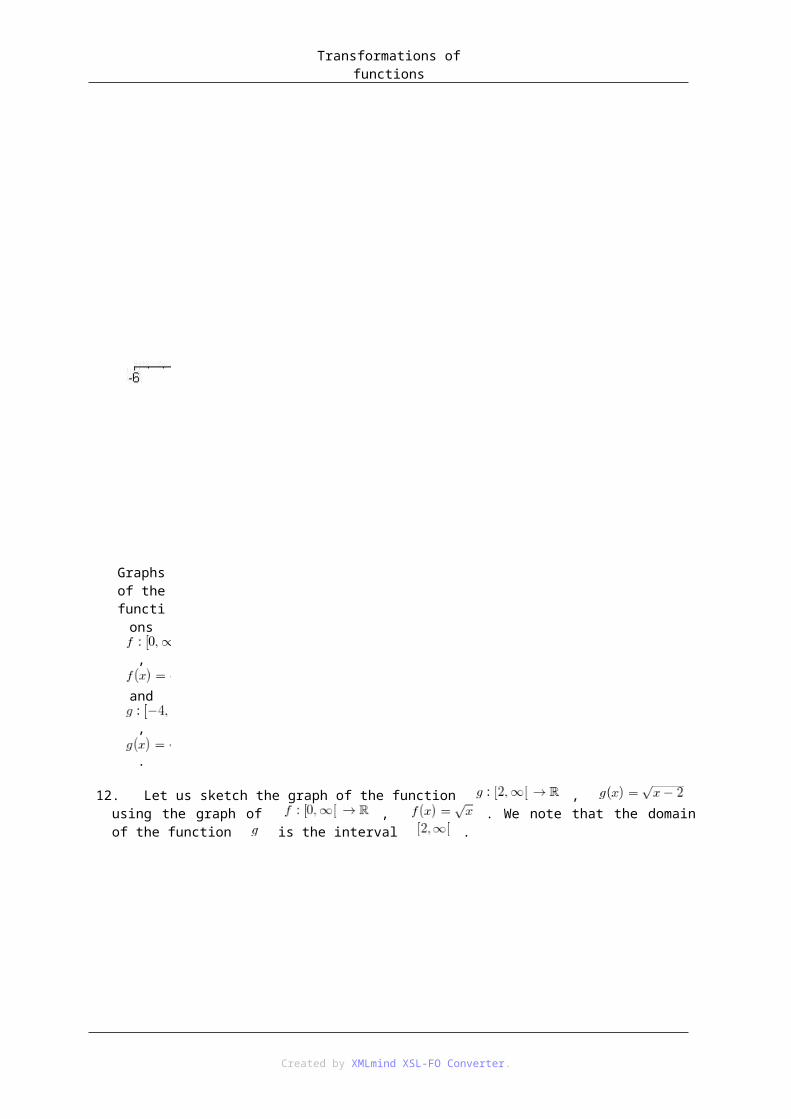
11. Let us sketch the graph of the function , using the graph of , . It is important to note here, that the domain of the function is
the interval .
Created by XMLmind XSL-FO Converter.

Transformations of functions
Graph of the
function
,
.
Created by XMLmind XSL-FO Converter.

Transformations of functions
Graphs of the
functions
,
and
,
.
12. Let us sketch the graph of the function , using the graph of , . We note that the domain of the function is the interval
.
Created by XMLmind XSL-FO Converter.

Transformations of functions
Graphs of the
functions
,
and
,
.
13. Let us sketch the graphs of the function , using the graph of , .
Created by XMLmind XSL-FO Converter.
Transformations of functions
Graph of the
function
,
.
Created by XMLmind XSL-FO Converter.

Transformations of functions
Graphs of the
functions
,
and
,
.
14. Let us sketch the graphs of the function , using the graph of , .
Created by XMLmind XSL-FO Converter.

Transformations of functions
Graphs of the
functions
,
and
,
.
15. Let us sketch the graphs of the function , using the graph of , .
Created by XMLmind XSL-FO Converter.
Transformations of functions
Graph of the
function
,
.
Created by XMLmind XSL-FO Converter.

Transformations of functions
Graphs of the
functions
,
and
,
.
16. Let us sketch the graphs of the function , using the graph of , .
Created by XMLmind XSL-FO Converter.

Transformations of functions
Graphs of the
functions
,
and
,
.
Exercise 4.1. Sketch the graph of the function function using the graph of in the case when
a) , , , ;
b) , , , ;
c) , , , ;
d) , , , ;
e) , , , ;
f) , , , ;
g) , , , ;
h) , , , ;
Created by XMLmind XSL-FO Converter.

Transformations of functions
i) , , , ;
j) , , , ;
k) , , , ;
l) , , , ;
m) , , , ;
n) , , , ;
o) , , , ;
p) , , , .
2. 4.2. Scaling graphs of functionsIn this section, we will study, how we can get the graph of the functions and from the graph of , where is a real constant.
Similarly to the previous part, we try to get some observations based on our knowledge of drawing graphs of functions.
First, we consider the transformation type ` ', and we start again with the graph of the simple quadratic function , .
Created by XMLmind XSL-FO Converter.

Transformations of functions
Graph of the
function
,
.
Let us consider the graph of , :
Graph of the
function
,
.
Finally, we sketch both functions in the same coordinate system:
Created by XMLmind XSL-FO Converter.
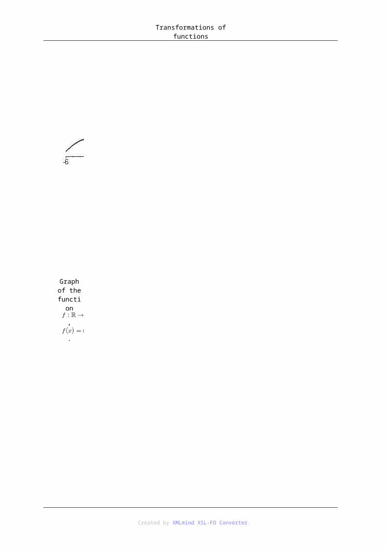
Transformations of functions
Graphs of the
functions
,
and
,
.
It is easy to see, that, we can get each point of the graph of using from the corresponding point of the graph . Since this property is valid for all pairs of points and of the graphs of our functions, we may obtain the graph of by stretching (or magnifying) the graph of the function with the factor vertically.
Let us investigate the function , now.
Created by XMLmind XSL-FO Converter.

Transformations of functions
Graph of the
function
,
.
Sketching and in the same coordinate system, we obtain:
Created by XMLmind XSL-FO Converter.

Transformations of functions
Graphs of the
functions
,
and
,
.
Here, each point of the graph of can be obtained by the calculation from the corresponding point of the graph . Therefore, we get the graph of the function by compressing (or shrinking) the graph of the function with the factor vertically.
It is important to note, that the sign of plays also here an important role.
Namely, the graph of , is:
Created by XMLmind XSL-FO Converter.

Transformations of functions
Graph of the
function
,
.
If we draw it together with the graph of , we get
Created by XMLmind XSL-FO Converter.

Transformations of functions
Graphs of the
functions
,
and
,
.
It is easy to see, that we can get the graph of by reflecting the graph of about the -axis.
If we would like to determine the graph of the function , , we have to combine the two steps above: we have to stretch (or magnify) the graph of the function with the factor
vertically, and we have to reflect this (new) graph about the -axis.
This situation is illustrated in the following picture.
Created by XMLmind XSL-FO Converter.

Transformations of functions
Graphs of the
functions
,
and
,
.
Let us investigate now the transformations of the type ` '. In the case of the function , , we have , therefore, it does not give new information for us in this
case By this reason, in the following, we will consider the function , us our `basis function'. The graph of this function is:
Created by XMLmind XSL-FO Converter.

Transformations of functions
Graph of the
function
,
.
Let us consider the graph of , .
Created by XMLmind XSL-FO Converter.

Transformations of functions
Graph of the
function
,
.
Sketching these two graphs in the same coordinate system, we get
Created by XMLmind XSL-FO Converter.
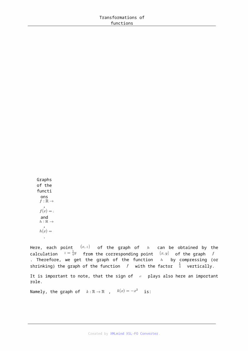
Transformations of functions
Graphs of the
functions
,
and
,
.
It is visible that we can get the graph of by stretching (or magnifying) the graph of by the factor horizontally.
The situation is analogous, if our constant is positive, but less than . In this case we compress (or shrinking) the graph instead of stretching (or magnifying) it.
We illustrate these situations with the functions and , . in the following pictures.
Created by XMLmind XSL-FO Converter.

Transformations of functions
Graph of the
function
,
.
Sketching these two graphs in the same coordinate system, we get
Created by XMLmind XSL-FO Converter.
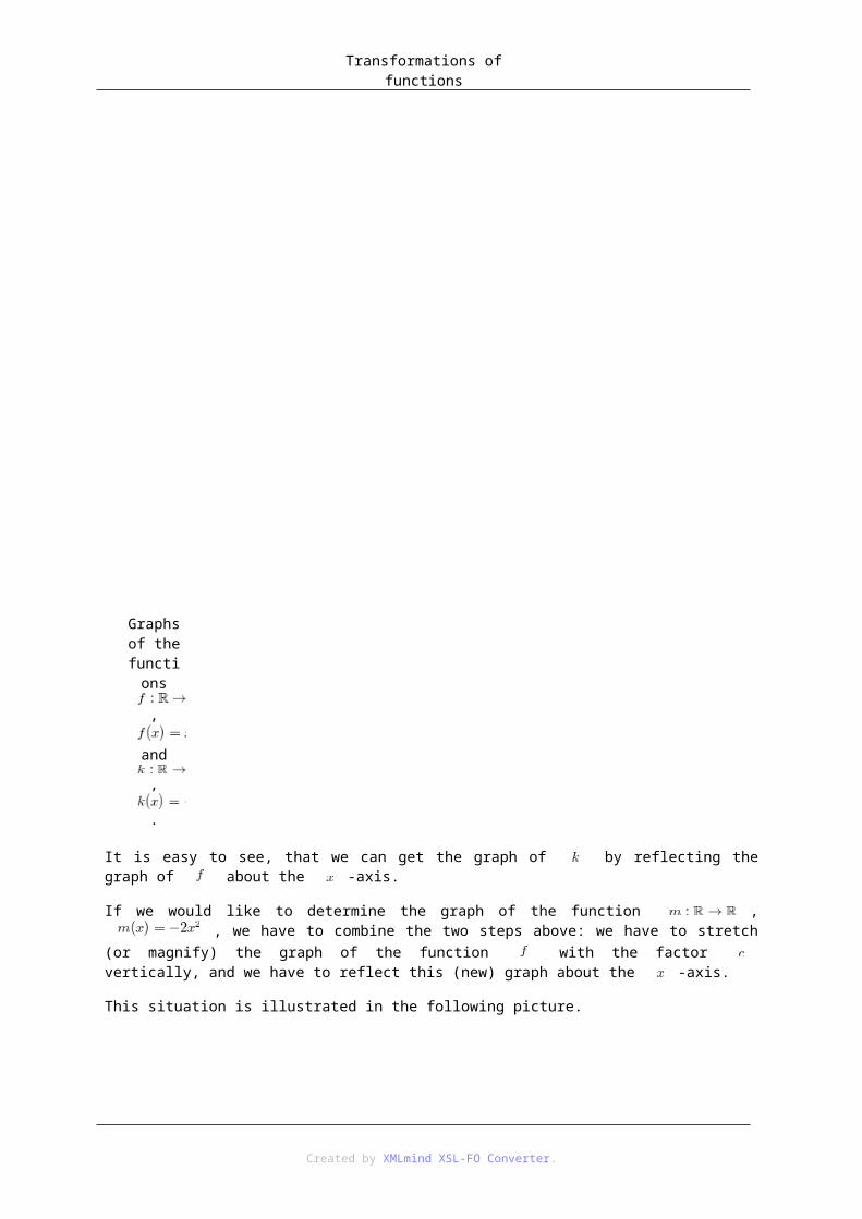
Transformations of functions
Graphs of the
functions
,
and
,
.
Finally, we will investigate the case when our factor is negative. Let us consider the function , .
Created by XMLmind XSL-FO Converter.

Transformations of functions
Graph of the
function
,
.
Created by XMLmind XSL-FO Converter.
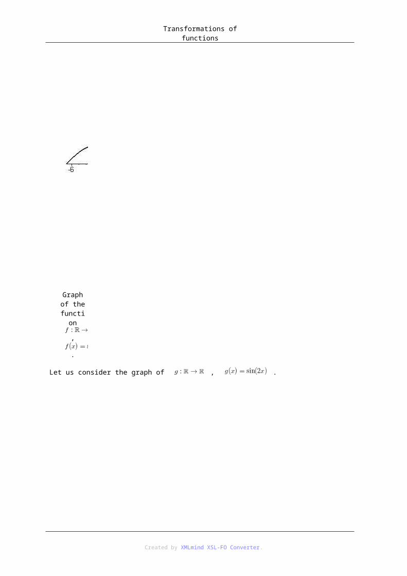
Transformations of functions
Graphs of the
functions
,
and
,
.
Similarly to the case of a `negative constant ' above, we easily get, that in this case, after stretching (or magnifying) or compressing (or shrinking) the graph of , we have to reflect the result about the -axis.
We illustrate this situation with the graphs of the functions , and , .
Created by XMLmind XSL-FO Converter.
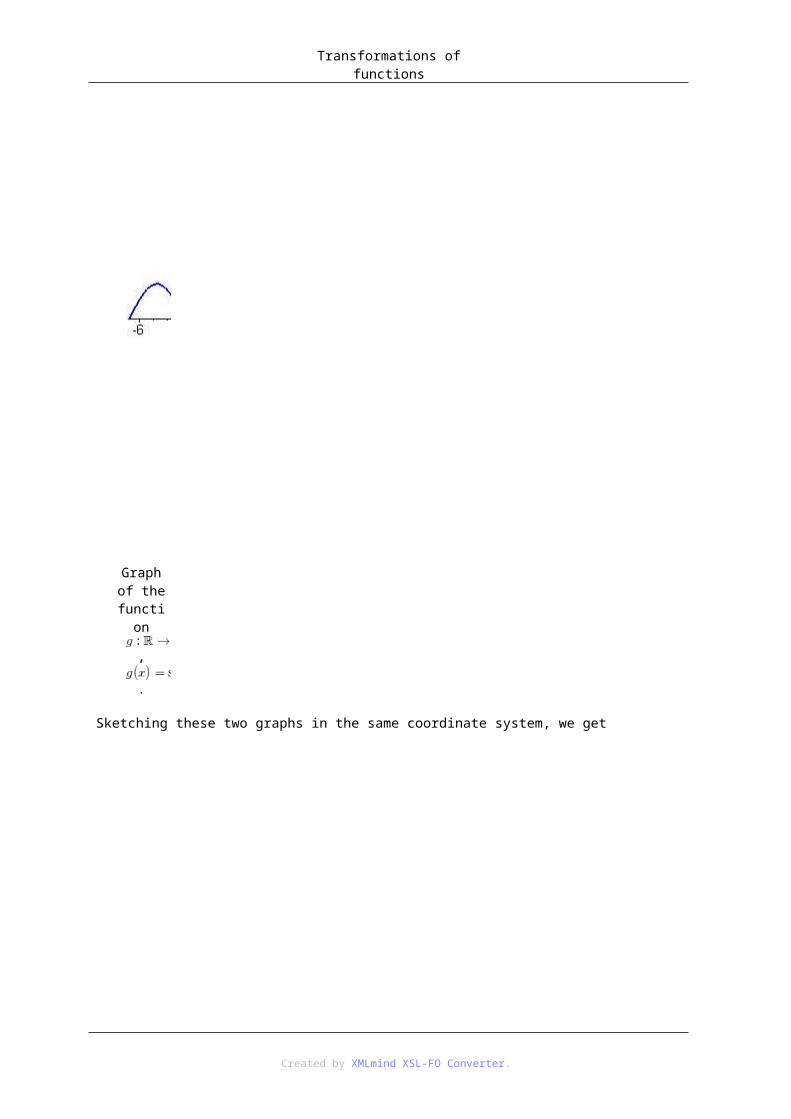
Transformations of functions
Graph of the
function
,
.
Created by XMLmind XSL-FO Converter.

Transformations of functions
Graphs of the
functions
,
and
,
.
It is clear that the argumentations above is independent from the concrete functions, it only depends on the connection between them. Thus, we can give a general method for these types of function transformations, too. In order describe this method, let be a set, let be a real number and denote the set .
Let be a real number, be a set and let us consider a function .
– In the case when , we can obtain the graph of the function , by stretching (or magnifying) the graph of the function with the factor vertically.
– In the case when , we can obtain the graph of the function , by compressing (or shrinking) the graph of the function with the factor vertically.
– In the case when , we can obtain the graph of the function , by stretching (or magnifying) the graph of the function with the factor vertically, and reflecting this graph about the -axis.
– In the case when , we can obtain the graph of the function ,
Created by XMLmind XSL-FO Converter.
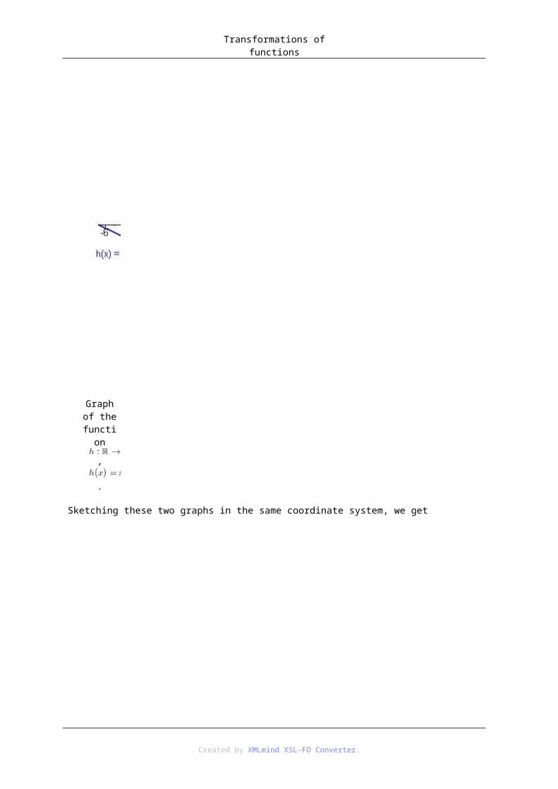
Transformations of functions
by compressing (or shrinking) the graph of the function with the factor vertically, and reflecting this graph about the -axis.
– In the case when , we can obtain the graph of the function , by stretching (or magnifying) the graph of the function with the factor horizontally.
– In the case when , we can obtain the graph of the function , by compressing (or shrinking) the graph of the function with the factor horizontally.
– In the case when , we can obtain the graph of the function , by stretching (or magnifying) the graph of the function with the factor horizontally, and reflecting this graph about the -axis.
– In the case when , we can obtain the graph of the function , by compressing (or shrinking) the graph of the function with the factor
horizontally, and reflecting this graph about the -axis.
Examples.
1. Let us sketch the graphs of the function , using the graph of , .
Graph of the
function
,
.
Created by XMLmind XSL-FO Converter.

Transformations of functions
Graphs of the
functions
,
and
,
.
2. Let us sketch the graphs of the function , using the graph of , .
Created by XMLmind XSL-FO Converter.

Transformations of functions
Graphs of the
functions
,
and
,
.
3. Let us sketch the graphs of the function , using the graph of , .
Created by XMLmind XSL-FO Converter.

Transformations of functions
Graphs of the
functions
,
and
,
.
4. Let us sketch the graphs of the function , using the graph of , .
Created by XMLmind XSL-FO Converter.

Transformations of functions
Graphs of the
functions
,
and
,
.
5. Let us sketch the graphs of the function , using the graph of , .
Created by XMLmind XSL-FO Converter.
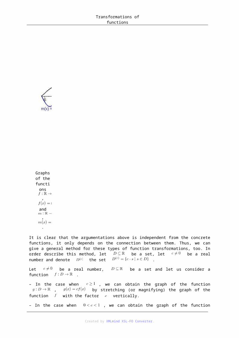
Transformations of functions
Graphs of the
functions
,
and
,
.
6. Let us sketch the graphs of the function , using the graph of , .
Created by XMLmind XSL-FO Converter.
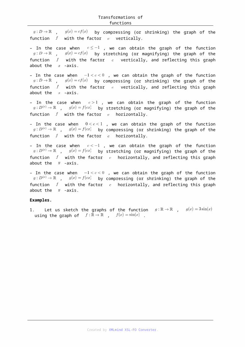
Transformations of functions
Graphs of the
functions
,
and
,
.
7. Let us sketch the graphs of the function , using the graph of , .
Created by XMLmind XSL-FO Converter.

Transformations of functions
Graphs of the
functions
,
and
,
.
8. Let us sketch the graphs of the function , using the graph of , .
Created by XMLmind XSL-FO Converter.
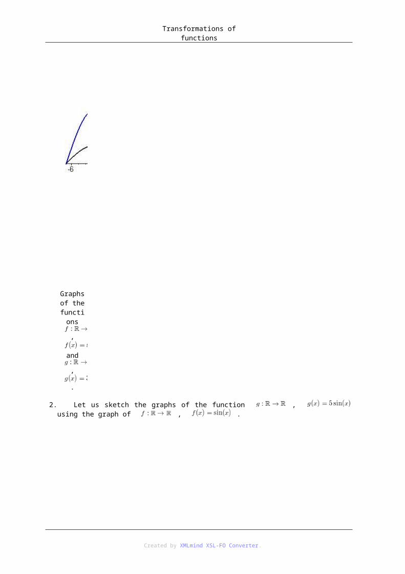
Transformations of functions
Graphs of the
functions
,
and
,
.
9. Let us sketch the graphs of the function , using the graph of , .
Created by XMLmind XSL-FO Converter.

Transformations of functions
Graphs of the
functions
,
and
,
.
10. Let us sketch the graphs of the function , using the graph of , .
Created by XMLmind XSL-FO Converter.

Transformations of functions
Graphs of the
functions
,
and
,
.
11. Let us sketch the graphs of the function , using the graph of , .
Created by XMLmind XSL-FO Converter.

Transformations of functions
Graphs of the
functions
,
and
,
.
12. Let us sketch the graphs of the function , using the graph of , .
Created by XMLmind XSL-FO Converter.

Transformations of functions
Graphs of the
functions
,
and
,
.
13. Let us sketch the graph of the function , using the graph of , .
Created by XMLmind XSL-FO Converter.

Transformations of functions
Graph of the
function
,
.
Created by XMLmind XSL-FO Converter.
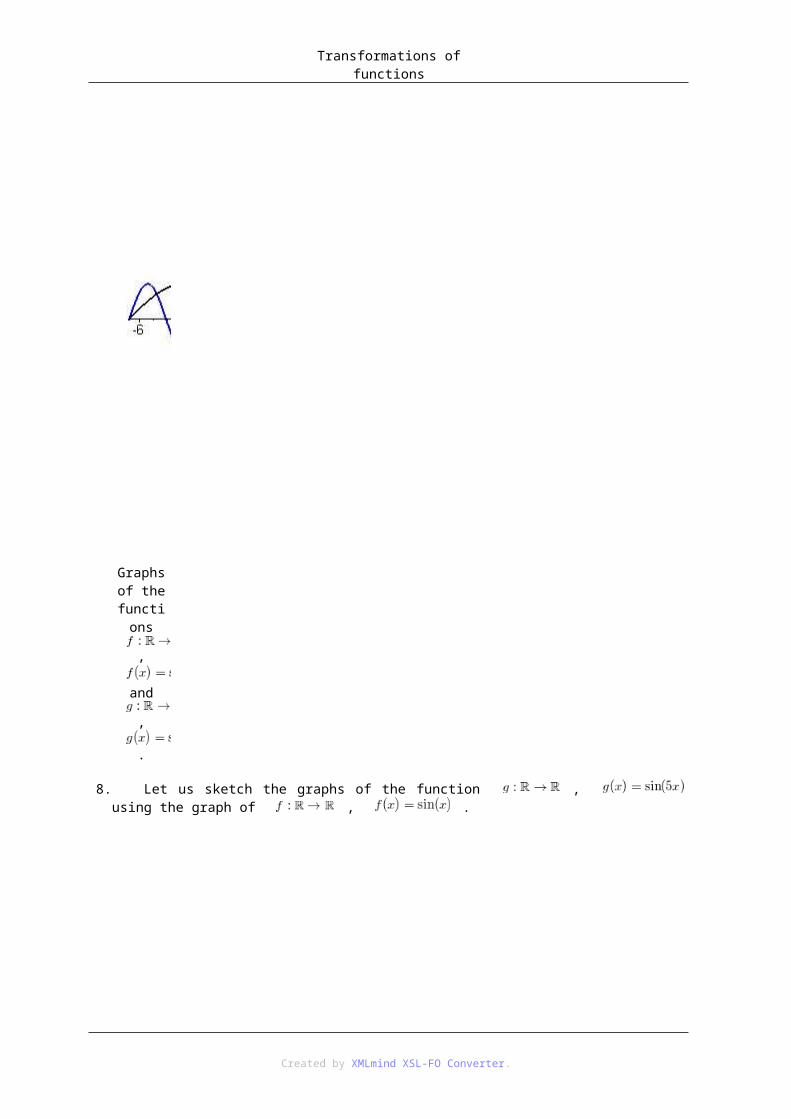
Transformations of functions
Graphs of the
functions
,
and
,
.
14. Let us sketch the graph of the function , using the graph of , .
Created by XMLmind XSL-FO Converter.

Transformations of functions
Graphs of the
functions
,
and
,
.
15. Let us sketch the graph of the function , using the graph of , .
Created by XMLmind XSL-FO Converter.

Transformations of functions
Graphs of the
functions
,
and
,
.
16. Let us sketch the graph of the function , using the graph of , .
Created by XMLmind XSL-FO Converter.

Transformations of functions
Graphs of the
functions
,
and
,
.
17. Let us sketch the graph of the function , using the graph of , .
Created by XMLmind XSL-FO Converter.

Transformations of functions
Graphs of the
functions
,
and
,
.
18. Let us sketch the graphs of the function , using the graph of , .
Created by XMLmind XSL-FO Converter.

Transformations of functions
Graphs of the
functions
,
and
,
.
19. Let us sketch the graphs of the function , using the graph of , .
Created by XMLmind XSL-FO Converter.
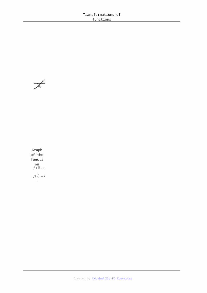
Transformations of functions
Graphs of the
functions
,
and
,
.
20. Let us sketch the graphs of the function , using the graph of , .
Created by XMLmind XSL-FO Converter.

Transformations of functions
Graphs of the
functions
,
and
,
.
21. Let us sketch the graphs of the function , using the graph of , .
Created by XMLmind XSL-FO Converter.

Transformations of functions
Graphs of the
functions
,
and
,
.
Exercise 4.2. Sketch the graph of the function function using the graph of in the case when
a) , , , ;
b) , , , ;
c) , , , ;
d) , , , ;
e) , , , ;
f) , , , ;
g) , , , ;
h) , , , ;
Created by XMLmind XSL-FO Converter.

Transformations of functions
i) , , , ;
j) , , , ;
k) , , , ;
l) , , , ;
m) , , , ;
n) , , , ;
o) , , , ;
p) , , , ;
q) , , , ;
r) , , , ;
s) , , , ;
t) , , , ;
Created by XMLmind XSL-FO Converter.

Chapter 5. Results of the exercises1. 5.1. Results of the Exercises of Chapter 1Solution of Exercise 1.1 [6]:
1. This part of the exercise is trivial, so we do not list the results.
2. The domain of the corresponding function is:
3.
4. The range of the corresponding function is:
Solution of Exercise 1.2 [8]
a)
Created by XMLmind XSL-FO Converter.
Results of the exercises
b)
c)
Created by XMLmind XSL-FO Converter.

Results of the exercises
d)
e)
Created by XMLmind XSL-FO Converter.

Results of the exercises
f)
g)
Created by XMLmind XSL-FO Converter.

Results of the exercises
h)
i)
Created by XMLmind XSL-FO Converter.

Results of the exercises
j)
k)
Created by XMLmind XSL-FO Converter.

Results of the exercises
l)
m)
Created by XMLmind XSL-FO Converter.

Results of the exercises
n)
o)
Created by XMLmind XSL-FO Converter.

Results of the exercises
p)
q)
Created by XMLmind XSL-FO Converter.

Results of the exercises
r)
Created by XMLmind XSL-FO Converter.
Results of the exercises
Solution of Exercise 1.3 [11]: In the cases a) and c) the curve is not the graph of a function, which is shown by the below application of the vertical line test:
a)
Created by XMLmind XSL-FO Converter.

Results of the exercises
c)
In exercises b) and d) the corresponding curve is the graph of a function.
Solution of Exercise 1.4 [14]
Created by XMLmind XSL-FO Converter.

Results of the exercises
The -intercept of the corresponding functions is:
The -intercepts of the corresponding functions are:
Solution of Exercise 1.5 [16]:
Created by XMLmind XSL-FO Converter.

Results of the exercises
Created by XMLmind XSL-FO Converter.

Results of the exercises
Solution of Exercise 1.6 [16]
Solution of Exercise 1.7 [42]
a) Let , and let , , , , , . We can illustrate in the following form:
Created by XMLmind XSL-FO Converter.

Results of the exercises
It is easy to see that is a function. It is also visible that there are no elements and such that , which implies that is injective. Since, for each element , there exists an such that , the function is also surjective. These properties imply that it is also bijective.
b) Let , and let , , , , , . We can illustrate in the following form:
It is obvious that is a function. Since , is not injective. Furthermore, there is no for which , thus is not surjective. This means that is not bijective.
c) Let , and let , , , , . We can illustrate in the following form:
Created by XMLmind XSL-FO Converter.

Results of the exercises
It is easy to se that is a function and it is injective. However, since there is no for which , the function is not surjective. This implies that is not bijective.
d) Let , and let , , , , , . We can illustrate in the following form:
It is visible that is a function and it is surjective. However is not injective, therefore, it is not bijective.
e) Let , and let , , , , , . We can illustrate in the following form:
Created by XMLmind XSL-FO Converter.

Results of the exercises
It is easy to see that is a function, it is injective, surjective, which implies that it is also bijective.
f) Let , and let , , , , , . We can illustrate in the following form:
It is visible that is a surjective function. However is not injective, therefore, it is not bijective.
Solution of Exercise 1.8 [43]
a) Let , . The graph of is:
Created by XMLmind XSL-FO Converter.

Results of the exercises
Graph of the
function
,
.
It is easy to see that there are no elements and in the domain of the function such that , which implies that is injective. It is also clear that, for each element of the range of the function , there exists an in the domain of such that , therefore, is surjective. These properties imply that is bijective.
b) Let , . The graph of is:
Created by XMLmind XSL-FO Converter.

Results of the exercises
Graph of the
function
,
.
It is easy to see that, similarly to the previous exercise, there are no elements and in the domain of the function such that , which yields that is injective. It is also clear
that, for each element of the range of the function , there exists an in the domain of with the property , therefore, is surjective. Thus, is bijective.
c) Let , . The graph of has the form:
Created by XMLmind XSL-FO Converter.

Results of the exercises
Graph of the
function
,
.
Similarly to the problems above, it is easy to verify that the function is injective and surjective, therefore, it is bijective.
d) Let , . The graph of has the form:
Created by XMLmind XSL-FO Converter.
Results of the exercises
Graph of the
function
,
.
Obviously, there are elements and in the domain of the function such that . (For example, .) Therefore is not injective. Furthermore,
there are elements in the range of the function , for which there does not exist any in the domain of with the property . (For example has this property.) This means that is not surjective. Since is neither injective nor surjective, it is not bijective.
e) Let , . The graph of has the form:
Created by XMLmind XSL-FO Converter.
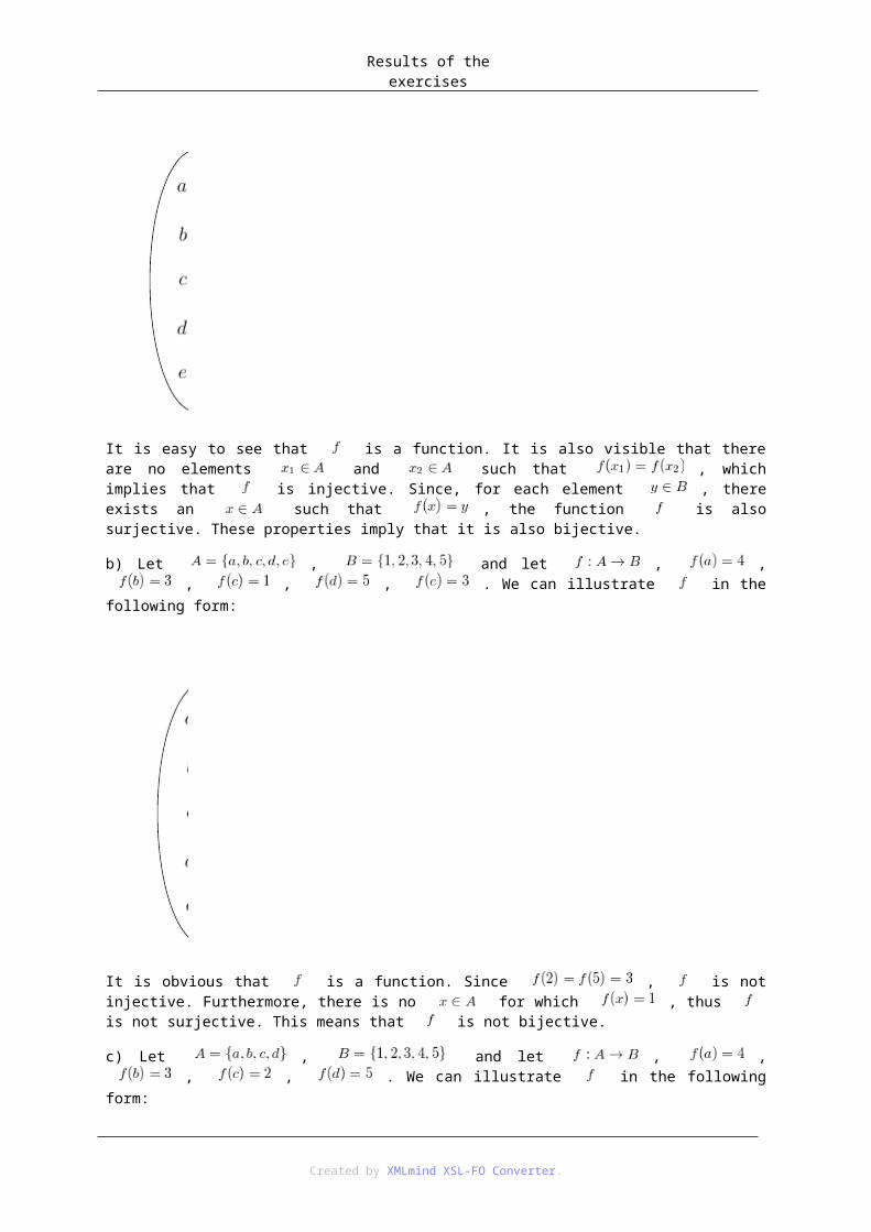
Results of the exercises
Graph of the
function
,
.
It is easy to see that, for each element of the range of , there exists an in the domain of such that , therefore, this function is surjective. However, similarly to the case above, there are elements and in the domain of the function such that
, which implies that is not injective. Since is not injective, it is not bijective.
f) Let , . The graph of has the form:
Created by XMLmind XSL-FO Converter.

Results of the exercises
Graph of the
function
,
.
Analogously to the exercise above, for each element of the range of , there exists an in the domain of such that , therefore, is surjective. Furthermore, there
are no elements and in the domain of such that , which implies that is injective. Since is surjective and injective, it is also bijective.
g) Let , . The graph of has the form:
Created by XMLmind XSL-FO Converter.
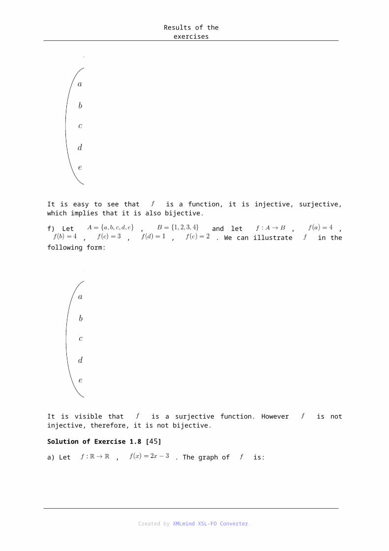
Results of the exercises
Graph of the
function
,
.
Similarly to the argumentation given in Exercise d above, it can be verified that the function is neither injective nor surjective, therefore, it is not bijective.
h) Let , . The graph of has the form:
Created by XMLmind XSL-FO Converter.

Results of the exercises
Graph of the
function
,
.
Similarly to Exercise e, we obtain that the function is surjective, but it is not injective, thus, it is not bijective.
i) Let , . The graph of has the form:
Created by XMLmind XSL-FO Converter.

Results of the exercises
Graph of the
function
,
.
Analogously to Exercise f, we may see that the function is surjective and injective and this implies that it is also bijective.
j) Let , . The graph of has the form:
Created by XMLmind XSL-FO Converter.

Results of the exercises
Graph of the
function
,
.
Similarly to the solution of the exercises above, we obtain that the function is neither injective nor surjective, therefore, it is not bijective.
k) Let , . The graph of has the form:
Created by XMLmind XSL-FO Converter.

Results of the exercises
Graph of the
function
,
.
It is easy to verify that the function is surjective, but it is not injective, thus, it is not bijective.
l) Let , . The graph of has the form:
Created by XMLmind XSL-FO Converter.

Results of the exercises
Graph of the
function
,
.
It is easy to see that the function is surjective and injective, therefore it is also bijective.
Solution of Exercise 1.9 [54]
a) Let , and let , , , , , . We may illustrate in the following form:
Created by XMLmind XSL-FO Converter.

Results of the exercises
It is easy to see that satisfies the requirements given in Definition 1.6 [2], thus, it is a function. Furthermore, is injective, thus, there exists its inverse. The inverse of has the form:
i. e.,
Created by XMLmind XSL-FO Converter.

Results of the exercises
which means that , , , , and .
b) Let , and let , , , , . We may illustrate as:
It is easy to see that an injective function, thus, there exists its inverse. The inverse of has the form:
Created by XMLmind XSL-FO Converter.

Results of the exercises
that is,
which means that , , , , .
c) Let , , , , , , . A diagram of is:
Created by XMLmind XSL-FO Converter.

Results of the exercises
It is visible that is a function and it is injective, therefore, it is invertible. Drawing `mechanically' the correspondence between the elements of the sets and , we obtain:
It is important to notify that the range of the function is the set , therefore, this set will be the domain of the inverse function of .
Created by XMLmind XSL-FO Converter.
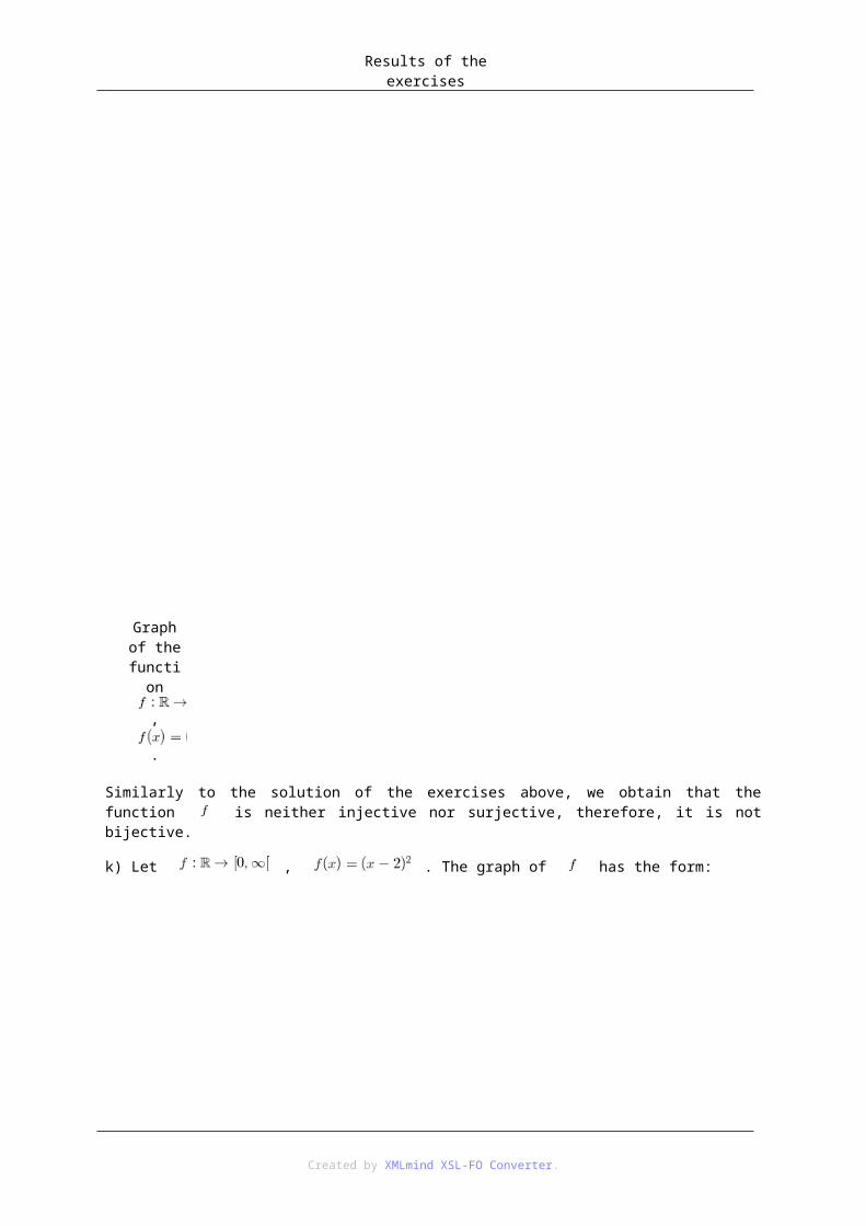
Results of the exercises
which gives that and , , , and .
d) Let , , , , , , , . A diagram of is:
It is easy to see that is a function, but it is not injective, since . Therefore, the inverse of does not exists.
Solution of Exercise 1.10 [55]
a) The graph of the function , is
Created by XMLmind XSL-FO Converter.
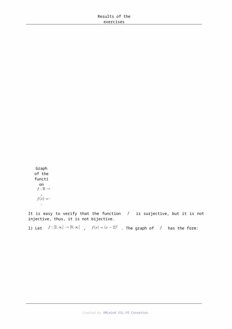
Results of the exercises
Graph of the
function
,
.
It is easy to see that this function is injective, therefore, it is invertible. Its inverse can be determined in the following form: by the definition of , we have for all , which gives
for each . Therefore, the inverse of is or, writing instead of , . The graph of
is:
Created by XMLmind XSL-FO Converter.

Results of the exercises
Graph of the
function
,
.
The graph of and its inverse in the same coordinate system
Created by XMLmind XSL-FO Converter.

Results of the exercises
Graphs of
,
and its inverse
,
.
b) The graph of , is
Created by XMLmind XSL-FO Converter.
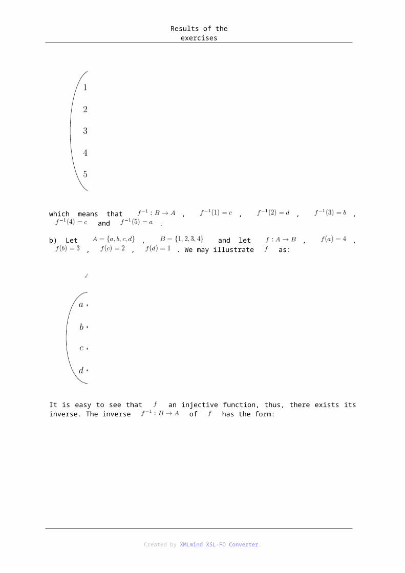
Results of the exercises
Graph of the
function
,
.
This function is injective, therefore, it is invertible. Its inverse can be obtained in the following form: for all , which yields for each . The inverse
of reads as or, writing instead of , . The graph of is:
Created by XMLmind XSL-FO Converter.

Results of the exercises
Graph of the
function
,
.
The graph of and its inverse is:
Created by XMLmind XSL-FO Converter.

Results of the exercises
Graphs of
,
and its inverse
,
.
c) The graph of the function , is:
Created by XMLmind XSL-FO Converter.
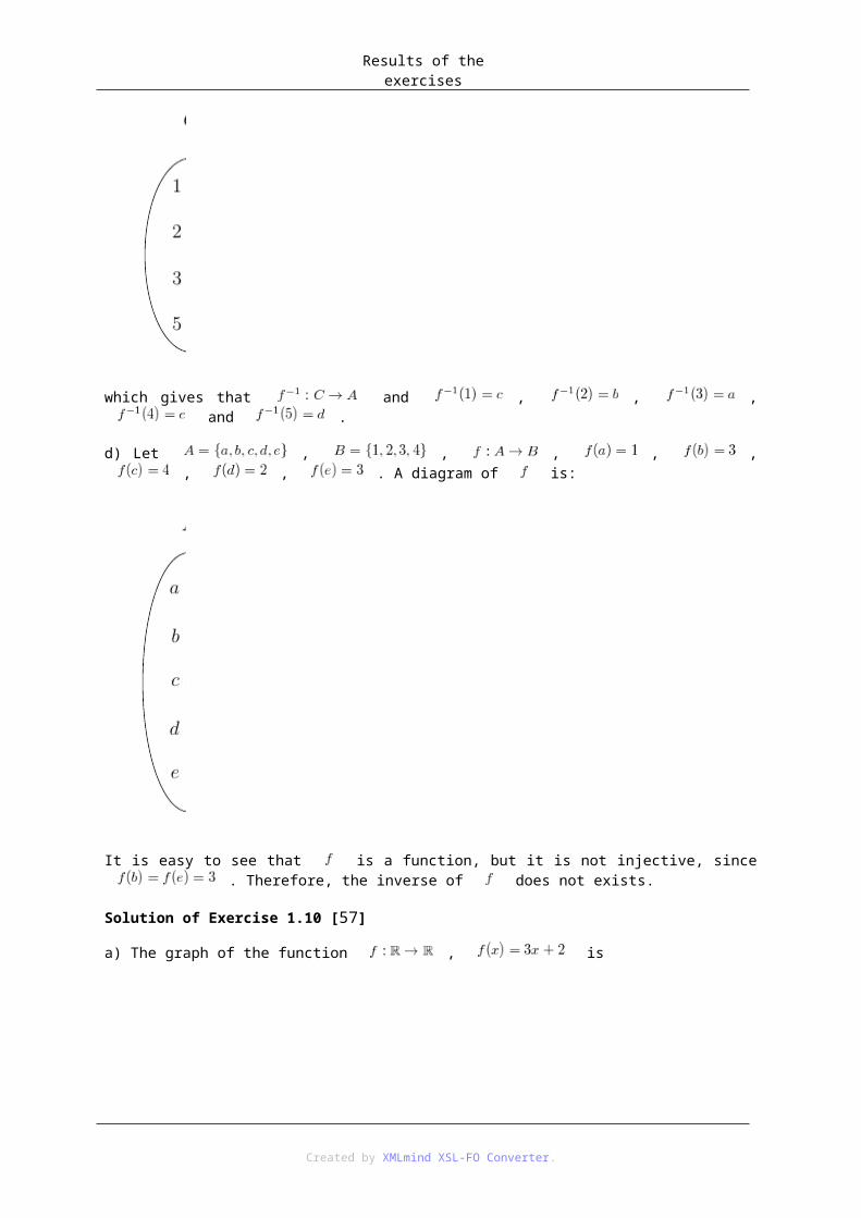
Results of the exercises
Graph of the
function
,
.
This function is not injective, therefore, it is not invertible.
d) The graph of , is
Graph of the
function
,
.
This function is injective, thus, it is invertible. Its inverse can be determined by the following calculation. The equation for all , gives for each . It is important to note that the range of is the set , therefore, this will be the domain of the inverse of . The inverse of is . Its graph is:
Created by XMLmind XSL-FO Converter.

Results of the exercises
Graph of the
function
,
.
The graphs of and its inverse is:
Created by XMLmind XSL-FO Converter.
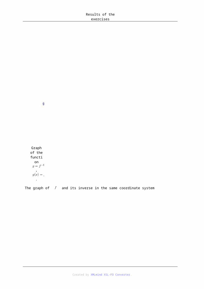
Results of the exercises
Graphs of
,
and its inverse
,
.
e) The graph of , is:
Created by XMLmind XSL-FO Converter.

Results of the exercises
Graph of the
function
,
.
The function is injective, thus, it is invertible. The range of is the set , thus, this set will be the domain of the inverse of . The of is
. Its graph is:
Created by XMLmind XSL-FO Converter.

Results of the exercises
Graph of the
function
,
.
The graphs of and are:
Created by XMLmind XSL-FO Converter.

Results of the exercises
Graphs of
,
and its inverse
,
.
f) The graph of , is:
Created by XMLmind XSL-FO Converter.

Results of the exercises
Graph of the
function
,
.
The function is injective, thus, it is invertible. The range of is the set , thus, this set will be the domain of the inverse of . The of is
. Its graph is:
Created by XMLmind XSL-FO Converter.

Results of the exercises
Graph of the
function
,
.
The graphs of and are:
Created by XMLmind XSL-FO Converter.

Results of the exercises
Graphs of
,
and its inverse
,
.
g) The graph of , is:
Created by XMLmind XSL-FO Converter.

Results of the exercises
Graph of the
function
,
.
The function is injective, thus, it is invertible. The range of is the set , thus, this set will be the domain of the inverse of . The of is
. Its graph is:
Created by XMLmind XSL-FO Converter.

Results of the exercises
Graph of the
function
,
.
The graphs of and are:
Created by XMLmind XSL-FO Converter.

Results of the exercises
Graphs of
,
and its inverse
,
.
2. 5.2. Results of the Exercises of Chapter 2Solution of Exercise 2.1 [60]:
The formula defining the corresponding functions is:
The graphs of the corresponding functions are:
a)
Created by XMLmind XSL-FO Converter.

Results of the exercises
b)
c)
Created by XMLmind XSL-FO Converter.
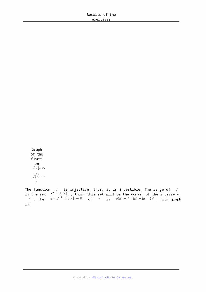
Results of the exercises
d)
Solution of Exercise 2.2 [60]:
Created by XMLmind XSL-FO Converter.

Results of the exercises
Solution of Exercise 2.3 [60]
Solution of Exercise 2.4 [64]:
1. The canonical form of the corresponding functions is:
2. The factorized form of the corresponding function (provided that ) is:
3. The -intercept is denoted by , and the -intercepts (if they exist at all) by and
Created by XMLmind XSL-FO Converter.
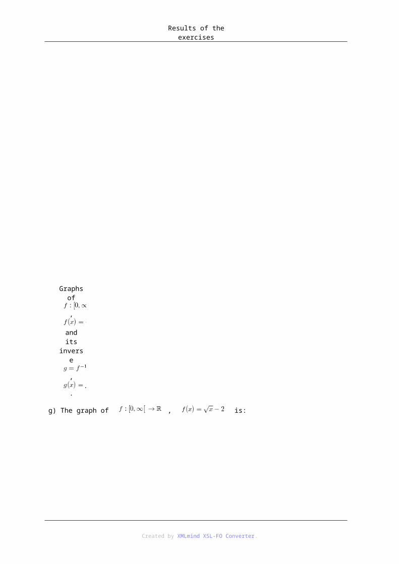
Results of the exercises
4. The vertex of the graph of the corresponding function is
5. The graph of is
a)
b)
Created by XMLmind XSL-FO Converter.

Results of the exercises
c)
d)
Created by XMLmind XSL-FO Converter.

Results of the exercises
e)
f)
Created by XMLmind XSL-FO Converter.

Results of the exercises
g)
h)
Created by XMLmind XSL-FO Converter.

Results of the exercises
i)
j)
Created by XMLmind XSL-FO Converter.

Results of the exercises
k)
l)
Created by XMLmind XSL-FO Converter.

Results of the exercises
m)
n)
Created by XMLmind XSL-FO Converter.

Results of the exercises
o)
p)
Created by XMLmind XSL-FO Converter.

Results of the exercises
Solution of Exercise 2.5 [66]:
The quotient and the remainder of the corresponding division is
Created by XMLmind XSL-FO Converter.

Results of the exercises
Solution of Exercise 2.6 [68]
3. 5.3. Results of the Exercises of Chapter 3Solution of Exercise 3.1 [90]:
Created by XMLmind XSL-FO Converter.

Results of the exercises
Solution of Exercise 3.2 [99]:
Created by XMLmind XSL-FO Converter.

Bibliography[1] K. A. Stroud and D. J. Booth. Engineering Mathematics, Sixth Edition. Industrial Press, Inc., New York.
2007.
[2] K. Sydsaeter and P. Hammond. Essential Mathematics for Economic Analysis, Third Edition. Prentice Hall, Harlow, London, New York. 2008.
[3] K. Sydsaeter, P. Hammond, A. Seierstad and A. Strom. Further Mathematics for Economic Analysis, Second Edition. Prentice Hall, Harlow, London, New York. 2008.
[4] G. B. Thomas, Jr., M. D. Weir and J. Hass. Thomas' Calculus, Early Transcendentals, Twelfth Edition. Addison–Wesley, Boston, Columbus, Indianapolis. 2009.
Created by XMLmind XSL-FO Converter.


![3. Numerical integration (Numerical quadrature). Given the continuous function f(x) on [a,b], approximate Newton-Cotes Formulas: For the given abscissas,](https://img.dokumen.tips/doc/110x75/56649e175503460f94b02909/3-numerical-integration-numerical-quadrature-given-the-continuous-function.jpg)