Reflections on Four Decades of CFD -- A Personal Perspectiveaero-comlab.stanford.edu/Papers/jrv_symposium_june2013/... · Introduction JST Scheme Fast Solver Moving Meshes Aerodynamic

Introduction JST Scheme Fast Solver Moving Meshes Aerodynamic Design Future Directions Conclusions Acknowledgments Appendix

Reflections on Four Decades of CFD –A Personal Perspective

Antony Jameson

Aerospace Computing LaboratoryDepartment of Aeronautics and Astronautics

Stanford University

A Symposium Celebrating the Careers ofAntony Jameson, Phil Roe and Bram van Leer

San Diego, CA

June 22-23, 2013

Antony Jameson Stanford University 0 / 74


Outline of the Talk

1 Introduction

2 Reflections on the JST Scheme

3 The Quest for a Fast Solver

4 Upwinding with Moving Meshes

5 Aerodynamic Design & Shape Optimization via Control Theory

6 Future Directions

7 Summary and Conclusions

8 Acknowledgments

9 Appendix



CFD Past, Present and Future



Influential People in My Life and Sponsors

Father Jacques St. Edmund’s School Shillong, IndiaSandy (Mr. Sanderson) Mowden School England

Dr. Hutton Winchester College EnglandWalter Oakeshott Winchester College England

Ernest Franke Trinity Hall, Cambridge EnglandArthur Shercliff Cambridge Engineering England

Sir William Hawthorne Cambridge Engineering England

Len Murray Trades Union Congress England

Rudy Meyer Grumman Aerospace USGrant Hedrick Grumman Aerospace US

Paul Garabedian Courant Institute US

Jerry C South Jr. NASA USMorton Cooper ONR USSpiro Lekoudis ONR USCharles Holland AFOSR USFariba Fahroo AFOSR US

Leland Jameson NSF US



Acknowledgments (1)

I am deeply honored to share this Symposium with Phil Roe and Bram Van Leer.Their work has provided the foundations of modern CFD methods, andprofoundly altered the evolution of the subject.

And I want to take this opportunity to thank Z. J. Wang for organizing theSymposium and Fariba Fahroo for her support.



Acknowledgments (2)

Aside from the contributions of my students to the research of our group, I amspecially indebted to them for their assistance in creating papers andpresentations in electronic form. In recent years I have been particularly helpedin this regard by

Kasidit LeoviriyakitNawee ButsuntornKui OuAndre ChanManuel LopezDavid Williams



History of CFD in Van Leer’s view



Emergence of CFD

In 1960 the underlying principles of fluid dynamics and the formulation of the governingequations (potential flow, Euler, RANS) were well established.

The new element was the emergence of powerful enough computers to make numericalsolution possible – to carry this out required new algorithms.

The emergence of CFD in the 1965 – 2005 period depended on a combination of advancesin computer power and algorithms.

Some significant developments in the 60s:

Birth of commercial jet transport – B707 & DC-8

Intense interest in transonic drag rise phenomena

Lack of analytical treatment of transonic aerodynamics

Birth of supercomputers – CDC6600

DC 8 Transonic Flow CDC 6600



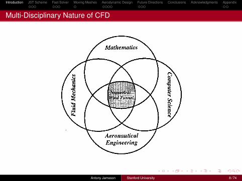
Multi-Disciplinary Nature of CFD



Hierarchy of Governing Equations



Reflections on the JST Scheme



Origins of the JST Scheme

The original JST scheme was developed in 1980-81 starting from a code that hadbeen developed at Dornier by Rizzi and Schmidt to solve the Euler equations

This code implemented the MacCormack scheme in finite volume form with additionalartificial dissipation to limit oscillations near shocks. It could not converge to a steadystate and it appeared from the Stockholm Workshop in 1979 that none of the existingEuler solvers could reach a steady state.

The primary objective of the JST scheme was to solve the steady state problem. Thisobjective was achieved through the use of blended low and high order artificialdissipation and modified Runge-Kutta time stepping with variable local time steps at afixed CFL number.

Note: The author had been experimenting with Euler solvers since 1976 and had achieved steady state

solutions for some simple geometries with the Z scheme. The code EUL1 still exists.



Original JST Scheme (1980)

The Dornier code (Rizzi-Schmidt) solved for w vol with MacCormack scheme + addeddiffusion

∼ δxεδxw vol, ε ∼˛p+1 − 2p + p−1

p+1 + 2p + p−1

˛It did not preserve uniform flow on a curvilinear grid.

In order to fix this, move vol outside δx.

Thenwn+1 = wn − ∆t

vol(Q−D), Q = convective terms

For dimensional consistency,

D ∼ δxvol

∆t∗δxw

where ∆t∗ is nominal time step

∆t∗ =vol

(Q+ cS)ı + (Q+ cS), Q = ~q · ~S

Higher order background diffusion was needed for convergence to a steady state.This had to be switched off in the vicinity of a shock to prevent oscillations.



Design Principles for the JST Scheme

Conservation: integral form=⇒finite volume scheme

Exact for uniform flow on a curvilinear grid=⇒constrains discretization, form of diffusion

Steady state independent of ∆tEliminates Lax-Wendroff, MacCormack schemes

Concurrent computationEliminates LU-SGS schemes =⇒ RK schemes

Non-oscillatory shock capturing=⇒switched artificial diffusion: upwind biasing

At least second order accurate=⇒first order diffusion coefficient ∼ ∆xp

Constant total enthalpy in steady flowEliminates Steger-Warming and other splittings

=⇒diffusion for energy equation ∼ ∂

∂xε∂

∂xρH

Simplicity



Mathematical Foundations for the JST Scheme: LED Scheme

A semi-discrete scheme is LOCAL EXTREMUM DIMINISHING (LED) if local maximacannot increase and local minima cannot decrease.A scheme in the form

dvıdt

=X6=ı

aı(v − vı)

is LED if

aı ≥ 0, aı = 0 if ı and are not neighbors.(compact stencil)

In one dimension an LED scheme is total variation diminishing (TVD). With the rightswitching strategy the JST scheme is LED for scalar conservation laws.



JST Results



JST Results for NACA 0012

VIS2=1 VIS2=0



The Quest for a Fast Solver



The Quest for a Fast Solver

Major aspects of aircraft design such as wing design require solutions of steady stateproblems.

A fast steady state solver may also be an important ingredient of an implicit schemefor unsteady flow.



Steady state Solutions and Implicit Schemes

Consider the semi-discrete system

dw

dt+R(w) = 0

where R(w) is the space residual which results from spatial discretization of the flowequations.

Any implicit scheme, for example the backward Euler scheme

wn+1 = wn −∆tR`wn+1´

requires the solution of a very large number of coupled nonlinear equations whichhave the same complexity as the steady state problem

R(w) = 0.

Accordingly a fast steady state solver is an essential building block for an implicitscheme.



Paradox



RANS Example

In current practice a steady flow over a wing is typically simulated with theReynolds Averaged Navier-Stokes (RANS) equations on a grid with 10 millioncells.

Using a two-equation turbulence model, this requires the solution of a system ofnonlinear equations with N = 70 million unknowns.

Even a linear problem of this size would require iterative solution, considering thatdirect inversion by Gaussian elimination would require order (N3) operations.

By taking advantage of sparsity this might be reduced to order (N2) with asophisticated direct solver, but a Newton iteration requiring the solution of asequence of linear problems of this size would still be very expensive.

No lower bound for the cost solving steady state problems has been established,but the author believes we should not be satisfied until they can be solved with nomore than 100 iterations, each with a cost of order N operations.



Multigrid Time Stepping Scheme

Towards this goal the author has focused on multigrid time stepping in a fullapproximation scheme (Jameson 1983)

For the Euler equations this approach has proved successful using1 Additive Runge-Kutta schemes designed to act as low pass filters (Jameson

1983, 1985)2 Variations of LU-SGS schemes (Yoon and Jameson 1988, Rieger and Jameson

1988, Jameson and Caughey 2001)

Euler solutions with engineering accuracy can be obtained in about 25 steps with RKschemes, and as few as 5 steps with SGS schemes.



Additive Runge Kutta schemes with enhanced stability region

To achieve large stability intervals along both axes it pays to treat the convective and dissipativeterms in a distinct fashion (Jameson 1985, 1986, Martinelli 1987).

Accordingly the residual is split asR(w) = Q(w) + D(w),

where Q(w) is the convective part and D(w) the dissipative part. Denote the time level n∆t by asuperscript n. Then the multistage time stepping scheme is formulated as

w(0)

= wn

w(1)

= w0 − α1∆t

“Q

(0)+ D

(0)”

w(2)

= w0 − α2∆t

“Q

(1)+ D

(1)”

. . .

w(k)

= w0 − αk∆t

“Q

(k−1)+ D

(k−1)”

. . .

wn+1

= w(m)

,

where the superscript k denotes the k-th stage, αm = 1, and

Q(0)

= Q“w

0”, D

(0)= β1D

“w

0”

. . .

Q(k)

= Q“w

(k)”

D(k)

= βk+1D“w

(k)”

+ (1− βk+1)D(k−1)

.




The coefficients αk are chosen to maximize the stability interval along the imaginary axis,and the coefficients βk are chosen to increase the stability interval along the negative realaxis.These schemes do not fall within the standard framework of Runge-Kutta schemes, andthey have much larger stability regions.Two particularly effective schemes are:

4-2 scheme

α1 = 13

β1 = 1.00

α2 = 415

β2 = 0.50

α3 = 59

β3 = 0.00α4 = 1 β4 = 0.00

(1)

5-3 schemeα1 = 1

4β1 = 1.00

α2 = 16

β2 = 0.00

α3 = 38

β3 = 0.56

α4 = 12

β4 = 0.00α5 = 1 β5 = 0.44

(2)

The figures on the next slide display the stability regions for the standard fourth order RK4scheme and the 4-2 and 5-3 schemes. The expansion of the stability region is apparent.The modified schemes have proved to be particularly effective in conjunction with multigrid.






RK-SGS Scheme

RK multigrid schemes are typically augmented by residual averaging (Jameson andBaker 1983) where at each stage the correction ∆w is smoothed implicitly.

In 1-D−ε∆wi+1 + (1 + 2ε)∆wi − ε∆wi−1 = ∆wi

and ∆w is used for the stage update.

Rossow (2006) proposed substituting LU-SGS preconditioning sweeps to modify thecorrection. This concept was further developed by Rossow, Swanson and Turkel(2007). They presented results obtained with 3 and 5 stage RK schemes using 3LU-SGS sweeps at each stage.

Accordingly the cost of each time step is much greater than that of a standard RKscheme.



RK-SGS Scheme

During the last year the present author has systematically investigated RK-SGSschemes using an alternate formulation of the LU-SGS preconditioner whileexchanging results with Swanson. Two schemes have emerged as best.

1 2-Stage Additive RK-SGS Scheme

α1 = 0.24 β1 = 1.00α2 = 1.0 β2 = 2

3

(3)

2 3-Stage Additive RK-SGS Scheme

α1 = 0.15 β1 = 1.00α2 = 0.4 β2 = 0.5α3 = 1.0 β3 = 0.5

(4)

Both schemes have proved robust with a single LU-SGS sweep at each stage,provided that the absolute eigenvalues used in the preconditioner are appropriatelybounded away from zero. Hence the computational cost of each time step is quite low.



Results of RK-SGS Scheme Combined with JST Scheme

ONERA M6 WingM = 0.84, α = 3.06, Re = 6× 106

5 Digit accuracy of CL and CD in 20 steps (Convergence Rate = 0.56)

15 Orders of magnitude reduction of residuals to machine zero in 130 steps (Convergence Rate = 0.77)



Results of RK-SGS Scheme Combined with JST Scheme

ONERA M6 WingM = 8.0, α = 10.0, Re = 6× 106

Solution in 150 steps (Convergence Rate = 0.92)

Needs extra dissipation during the first 80 steps to avoid negative pressure near the wing tip.



Upwinding with Moving Meshes



Upwinding with Moving Meshes

With mesh velocity s∂w

∂t+

∂

∂x(f(w)− sw) = 0

Scheme (1)Upwind based on sign of eigenvalues based on relative velocity

u− s

u− s+ c

u− s− c

Scheme (2)Upwinding of flux f(w) with absolute eigenvalues

u

u+ c

u− cseparate upwinding of mesh term sw based on sign of s



Shock Tube Problem



Aerodynamic Design&

Shape Optimizationvia

Control Theory



Aerodynamic Design Process

The Aerodynamic Design Process



Aerodynamic Design Based on Control Theory

Regard the wing as a device to generate lift (with minimum drag) by controllingthe flow

Apply theory of optimal control of systems governed by PDEs (Lions) withboundary control (the wing shape)

Merge control theory and CFD

Find the Frechet derivative (infinite dimensional gradient) of a cost function(performance measure) with respect to the shape by solving the adjoint equationin addition to the flow equation

Modify the shape in the sense defined by the smoothed gradient

Repeat until the performance value approaches an optimum



Aerodynamic Shape Optimization: Gradient Calculation

For the class of aerodynamic optimization problems under consideration, the designspace is essentially infinitely dimensional. Suppose that the performance of a systemdesign can be measured by a cost function I which depends on a function F(x) thatdescribes the shape,where under a variation of the design δF(x), the variation of thecost is δI. Now suppose that δI can be expressed to first order as

δI =

ZG(x)δF(x)dx

where G(x) is the gradient. Then by setting

δF(x) = −λG(x)

one obtains an improvement

δI = −λZG2(x)dx

unless G(x) = 0. Thus the vanishing of the gradient is a necessary condition for alocal minimum.



Aerodynamic Shape Optimization: Gradient Calculation

Computing the gradient of a cost function for a complex system can be a numericallyintensive task, especially if the number of design parameters is large and the costfunction is an expensive evaluation. The simplest approach to optimization is to definethe geometry through a set of design parameters, which may, for example, be theweights αi applied to a set of shape functions Bi(x) so that the shape is representedas

F(x) =X

αiBi(x).

Then a cost function I is selected which might be the drag coefficient or the lift to dragratio; I is regarded as a function of the parameters αi. The sensitivities ∂I

∂αimay now

be estimated by making a small variation δαi in each design parameter in turn andrecalculating the flow to obtain the change in I. Then

∂I

∂αi≈ I(αi + δαi)− I(αi)

δαi.



Symbolic Development of the Adjoint Method

Let I be the cost (or objective) function

I = I(w,F)

where

w = flow field variables

F = grid variables

The first variation of the cost function is

δI =∂I

∂w

T

δw +∂I

∂F

T

δF

The flow field equation and its first variation are

R(w,F) = 0

δR = 0 =

»∂R

∂w

–δw +

»∂R

∂F

–δF



Symbolic Development of the Adjoint Method (cont.)

Introducing a Lagrange Multiplier, ψ, and using the flow field equation as aconstraint

δI =∂I

∂w

T

δw +∂I

∂F

T

δF − ψT»

∂R

∂w

–δw +

»∂R

∂F

–δFff

=

∂I

∂w

T

− ψT»∂R

∂w

–ffδw +

∂I

∂F

T

− ψT»∂R

∂F

–ffδF

By choosing ψ such that it satisfies the adjoint equation»∂R

∂w

–Tψ =

∂I

∂w,

we have

δI =

∂I

∂F

T

− ψT»∂R

∂F

–ffδF

This reduces the gradient calculation for an arbitrarily large number of designvariables at a single design point to=⇒ One Flow Solution + One Adjoint Solution



Gradient SmoothingConsider a shape change f(x) =⇒ f + δf

Set δf = −λg to obtain

δI =

Zg δf dx = −λ

Zg2dx

A smoothed gradient g is defined by

g −∂

∂xε∂g

∂x= g

and g = 0 at the end points.

Now setδf = −λg

Then

δI = −λZ „

g −∂

∂xε∂g

∂x

«gdx

= −λZ „

g2

+ ε

„∂g

∂x

«2«gdx

Note:1 If g = 0 then g = 0.

2 The smoothed gradient is the gradient with respect to a Sovolev inner product.

< u, v >=

Z `uv + εu

′v′´dx



Constraints

Fixed CL.

Fixed span load distribution to present too large CL on the outboard wing whichcan lower the buffet margin.

Fixed wing thickness to prevent an increase in structure weight.

- Design changes can be limited to a specific spanwise range of the wing.- Section changes can be limited to a specific chordwise range.

Smooth curvature variations via the use of Sobolev gradient.



Shock free airfoil design

The search for profiles which give shock free transonic flows was the subject ofintensive study in the 1965-70 period.

Morawetz’ theorem (1954) states that a shock free transonic flow is an isolatedpoint. Any small perturbation in Mach number, angle of attack, or shape causes ashock to appear in the flow.

Nieuwland generated shock free profiles by developing solutions in thehodograph plane. The most successful method was that developed byGarabedian and his co-workers. This used complex characteristics to developsolution in the hodograph plane, which was then mapped to the physical plane. Itwas hard to find hodograph solutions which mapped to physical realizable closedprofiles. It generally took one or two months to produce an acceptable solution.

By using shape optimization to minimize the drag coefficient at a fixed lift, shockfree solutions can be found in less than one minute.



Two dimensional studies of transonic airfoil design(cont’d)

Pressure distribution and Mach contours for the GAW airfoil

Before the redesign After the redesign



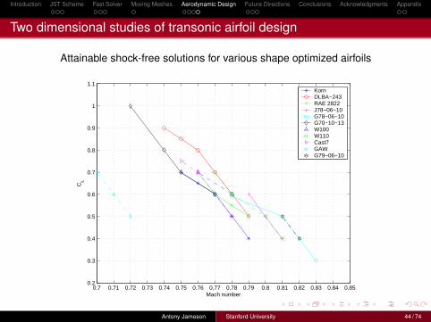
Two dimensional studies of transonic airfoil design

Attainable shock-free solutions for various shape optimized airfoils

0.7 0.71 0.72 0.73 0.74 0.75 0.76 0.77 0.78 0.79 0.8 0.81 0.82 0.83 0.84 0.850.2

0.3

0.4

0.5

0.6

0.7

0.8

0.9

1

1.1

Mach number

CL

KornDLBA−243RAE 2822J78−06−10G78−06−10G70−10−13W100W110Cast7GAWG79−06−10



Viscous Korn Airfoil Design

Initial Final



Viscous Korn Airfoil Design

Unsmoothed Smoothed



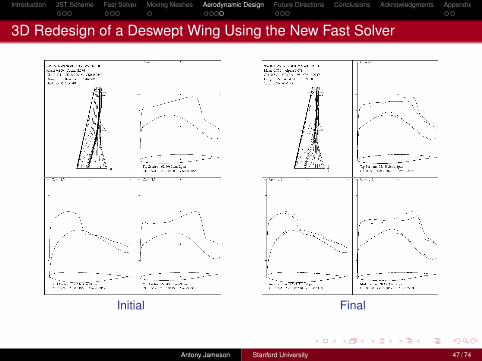
3D Redesign of a Deswept Wing Using the New Fast Solver

Initial Final



Future Directions



The Current Status of CFD

Worldwide commercial and government codes are based on algorithmsdeveloped in the 80s and 90s.

These codes can handle complex geometry but are generally limited to 2nd orderaccuracy.

They cannot handle turbulence without modeling.

Unsteady simulations are very expensive, and questions over accuracy remain.



CFD Contributions to B787



CFD Contributions to A380



The Future of CFD

CFD has been on a plateau for the past 15 years.

Representations of current state of the art:Formula 1 carsComplete aircrafts

The majority of current CFD methods are not adequate for vortex dominated andtransitional flows:

RotorcraftHigh-lift systemsFormation flying

In order to address these currently intractable problems we need to movetowards higher fidelity simulations with large eddy simulation (LES), or ultimatelydirect numerical simulation (DNS).



Large Eddy Simulation

The number of DoF for an LES of turbulent flow over an airfoil scales as Re1.8c (resp.Re0.4c ) if the inner layer is resolved (resp. modeled)

Rapid advances in computer hardware should make LES feasible within theforeseeable future for industrial problems at high Reynolds numbers. To realizethis goal requires

High-order algorithms for unstructured meshes (complex geometries)

Sub-Grid Scale models applicable to wall bounded flows

Massively parallel implementation



High Order Methods

At the Stanford Aerospace Computing Laboratory we have been focusing on the fluxreconstruction mehtod first proposed by H. T. Huynh (2007), which provides a unifying

framework for a variety of methods.



Recent Publications from the Stanford Aerospace ComputingLaboratory on High Order Methods

1 Castonguay, P., D. Williams, P. Vincent, M. Lopez, and A. Jameson (2011). On the development of ahigh-order, multi-GPU enabled, compressible viscous flow solver for mixed grids. AIAA P., vol.2011-3229

2 Jameson, A. (2010). A proof of the stability of the spectral difference method for all orders of accuracy. J.Sci. Comput., vol. 45(1)

3 Jameson, A. (2011). Advances in bringing high-order methods to practical applications in computationalfluid dynamics. AIAA P., vol. 2011-3226

4 Ou, K. and A. Jameson (2011). Unsteady adjoint method for the optimal control of advection andBurgers equations using high-order spectral difference method. AIAA P., vol. 2011- 24

5 Vincent, P. and A. Jameson (2011). Facilitating the adoption of unstructured high-order methodsamongst a wider community of fluid dynamicists. Math. Model. Nat. Phenom., vol. 6(3)

6 Vincent, P., P. Castonguay, and A. Jameson (2010). A new class of high-order energy stable fluxreconstruction schemes. J. Sci. Comput., vol. 47(1)

7 Vincent, P., P. Castonguay, and A. Jameson (2011). Insights from von Neumann analysis of high-orderflux reconstruction schemes. J. Comput. Phys., vol. 230(22)

8 Williams, D., P. Castonguay, P. Vincent, and A. Jameson (2011). An extension of energy stable fluxreconstruction to unsteady, non-linear, viscous problems on mixed grids. AIAA P., vol. 2011-3405

9 Lodato, G., P. Castonguay, and A. Jameson, Structural LES modeling with high-order spectral differenceschemes. In Annual Research Briefs (Center for Turbulence Research, Stanford University, 2011)

10 Jameson, A., P. Vincent, and P. Castonguay (2012). On the non-linear stability of flux reconstructionschemes. J. Sci. Comput., vol. 50(2)



The Flux Reconstruction Scheme

The solution is locally represented by Lagrange polynomial of degree n− 1 on thesolution points:

uh =nPj=1

uj lj(x) fDh =nPj=1

fDj lj(x)

The flux is discontinuous and needs to be corrected in a suitable way.

∆L = fL − fDh (−1) ∆R = fR − fDh (1)gL(−1) = 1, gL(1) = 0 gR(1) = 1, gR(−1) = 0

The continuous flux is obtained from the discontinuous counterpart by adding thecorrection functions of degree n weighted by the flux corrections.

fCh =

nXj=1

fDj lj(x) + gL(x)∆L + gR(x)∆R

The continuous flux is finally differentiated at the solution points and the solution isadvanced in time.

∂ui∂t

+

"nXj=1

fDjdljdx

(xi) + ∆LdgLdx

(xi) + ∆RdgRdx

(xi)

#= 0

Huynh (2007), AIAA Paper 2007-4079; Huynh (2009), AIAA Paper 2009-403



Energy Stability of the FR Scheme

The FR method defines a family of energy stable schemes in the norm.

‚‚‚UδD‚‚‚p,2

=

"NXn=1

Z xn+1

xn

“UδDn

”2

+c

2(Jn)2p

„∂pUδDn∂xp

«2

dx

# 12

The schemes have the form

∂ui∂t

+

"nXj=1

fDjdljdx

(xi) + ∆LdhLdx

(xi) + ∆RdhRdx

(xi)

#= 0

where the correction functions in terms of Legendre polynomials are

hL =(−1)p

2

»Lp −

„ηp(c)Lp−1 + Lp+1

1 + ηp(c)

«–

hR =(+1)p

2

»Lp +

„ηp(c)Lp−1 + Lp+1

1 + ηp(c)

«–with a single parameter c

ηp(c) =c(2p+ 1)(app!)

2

2Vincent, et al. (2010), J. Sci. Comput., 47(1); Vincent, et al. (2011), J. Comput. Phys., 230(22)



A Family of Energy Stable Schemes

Nodal DG:

c = 0 ⇒ ηp = 0

gL =(−1)p

2[Lp − Lp−1], gR =

(+1)p

2[Lp + Lp+1]

Spectral Difference:

c =2p

(2p+ 1)(p+ 1)(app!)2⇒ ηp =

p

p+ 1

gL =(−1)p

2(1− x)Lp, gR =

(+1)p

2(1 + x)Lp

G2 Scheme by Huynh [2007]:

c =2(p+ 1)

(2p+ 1)p(app!)2⇒ ηp =

p+ 1

p

gL =(−1)p

2

»Lp −

(p+ 1)Lp−1 + pLp+1

2p+ 1

–,

gR =(+1)p

2

»Lp +

(p+ 1)Lp−1 + pLp+1

2p+ 1

–



Study of Flapping Wing Sections

SD, 2D, N=5 on deforming grid

ExperimentJones, et al. (1998), AIAA J., 36(7)

NACA0012Re = 1850,Ma = 0.2, St = 1.5,

ω = 2.46, h = 0.12c



Flapping Wing Aerodynamics

Iso-Entropy colored by MaFlapping NACA 0012

Re = 2000, SD, N = 5, 4.7× 106 DoF

Iso-Entropy colored by MaWing-Body

Re = 5000, SD, N = 4, 2.1× 107 DoF

Ou, et al. (2011), AIAA Paper 2011-1316; Ou and Jameson (2011), AIAA Paper 2011-3068



Transitional Flow over SD7003 Airfoil

Iso-Entropy colored by MaWing-Body

Re = 5000, SD, N = 4, 2.1× 107 DoF

Castonguay, et al. (2010), AIAA Paper 2010-4626; Radespiel, et al. (2007), AIAA J., 45(6); Ol, et al. (2005), AIAA Paper 2005-5149; Galbraith,

Visbal (2008), AIAA Paper 2008-225; Uranga, et al. (2009), AIAA Paper 2009-4131;



Flow Over Spheres

Mach Contours + StreamlinesFlow over a spinning sphere,

Re = 300, Ma = 0.2

Iso-Entropy colored by MaFlow over a sphere

Re = 10000, Ma = 0.2

Ou, et al. (2011), AIAA Paper 2011-3668



Flow Past Counter-Rotating Cylinder Pair: ReD = 150, ω = 3.1Ω

SD, 4th Order, Ma = 0.2 Experiment (Princeton)

Chan et al. (2011), J. Fluid Mech., Vol. 679, pp. 343-382



Large Eddy Simulation of Flow Past Square Cylinder: ReD = 21400

Time integration: RK3

No. of elements: 35760 (2.3× 106DoF )

Grid dimensions: 21D× 12D× 3.2D

Reynolds: 21400

Mach: 0.3

Statistics: 16T0



Large Eddy Simulation of Flow Past Square Cylinder: ReD = 21400



Summary and Conclusions

Predicting the future is generally ill advised.However, the following are the author’s opinions:

The early development of CFD in the Aerospace Industry was primarily driven bythe need to calculate steady transonic flows: this problem is quite well solved.

CFD has been on a plateau for the last 15 years with 2nd-order accurate FVmethods for the RANS equations almost universally used in both commercial andgovernment codes which can treat complex configurations.

These methods cannot reliably predict complex separated, unsteady and vortexdominated flows.

Ongoing advances in both numerical algorithms and computer hardware andsoftware should enable an advance to LES for industrial applications within theforeseeable future.

Research should focus on high-order methods with minimal numerical dissipationfor unstructured meshes to enable the treatment of complex configurations.

Eventually DNS may become feasible for high Reynolds number flows...

hopefully with a smaller power requirement than a wind tunnel.



Acknowledgments

The current research is a combined effort by

Postdocs: Charlie Liang, Peter Vincent, Guido Lodato

Ph.D. students: Sachin Premasuthan, Kui Ou, Patrice Castonguay, DavidWilliams, Yves Alleneau, Lala Li, Manuel Lopez and Andre Chan

It is made possible by the support of

The Airforce Office of Scientific Research under grant FA9550-10-1-0418 by Dr.Fariba Fahroo

The National Science Foundation under grants 0708071 and 0915006 monitoredby Dr. Leland Jameson



Appendix



Artificial Diffusion and LED Schemes

Suppose that the scalar conservation law

∂v

∂t+

∂

∂xf(v) = 0

is approximated by the semi-discrete scheme

∆xdvdt

+ h+ 12− h− 1

2= 0 j j+1

hj−1/2

hj+1/2

j−1

where the numerical flux is

h+ 12

=1

2(f+1 + f)− α+ 1

2(v+1 − v)

Define a numerical estimate of the wave speed a(v) = ∂f∂v

as

a+ 12

=

8><>:f+1−f

v+1−v, v+1 6= v

∂f∂v|v , v+1 = v



Artificial Diffusion and LED Schemes (continued)

then the numerical flux

h+ 12

= f +1

2(f+1 − f)− α+ 1

2(v+1 − v)

= f −„α+ 1

2− 1

2a+ 1

2

«(v+1 − v)

and

h− 12

= f −1

2(f − f−1)− α− 1

2(v − v−1)

= f −„α− 1

2+

1

2a− 1

2

«(v − v−1)

The semi-discrete scheme then reduces to∆x

dvdt

= (α+ 12− 1

2a+ 1

2)(v+1 − v)− (α− 1

2+ 1

2a− 1

2)(v − v−1)

This is LED if α+ 12≥ 1

2|a+ 1

2| ∀.



Jameson-Schmidt-Turkel (JST) Scheme

This scheme blends low and high order diffusion.Suppose that the scalar conservation law

∂v

∂t+

∂

∂xf(v) = 0

is approximated by the semi-discrete scheme

∆xdvdt

+ h+ 12− h− 1

2= 0 j j+1

hj−1/2

hj+1/2

j−1

In the JST scheme, the numerical flux is

h+ 12

=1

2(f+1 + f)− d+ 1

2

where the diffusive flux has the form

d+ 12

= ε(2)

+ 12∆v+ 1

2− ε(4)

+ 12(∆v+ 3

2− 2∆v+ 1

2+ ∆v− 1

2)

with∆v+ 1

2= v+1 − v



JST Scheme

Let a+ 12

be an estimate of the wave speed ∂f∂v

a+ 12

=f+1 − fv+1 − v

or∂f

∂v|v=v if v+1 = v

Theorem: The JST scheme is LED if whenever v or v+1 is an extremum

ε(2)

+ 12≥ 1

2|a+ 1

2|, ε

(4)

+ 12

= 0

Proof: At an extremum the scheme reduces to

∆xdvdt

=

„ε(2)

+ 12− 1

2a+ 1

2

«∆v+ 1

2−„ε(2)

− 12

+1

2a− 1

2

«∆v− 1

2

where each term in parenthesis ≥ 0.



JST Scheme at a Maximum

The condition that ε(4)+ 1

2= 0 if v or v+1 is an extremum

=⇒ ε(4)

+ 12

= ε(4)

− 12

= 0.

(4)εj+1/2 =0=0

j+2j+1jj−1j−2

j−1/2(4)ε

Hence the scheme reduces to a 3-point scheme and

dvdt≤ 0

ifε(2)

+ 12≥ 1

2|a+ 1

2|, ε

(2)

− 12≥ 1

2|a− 1

2|,

since then the coefficients multiplying (v+1 − v) and (v−1 − v) are both ≥ 0.



Switch for JST Scheme

Define

R(u, v) =

˛u− v|u|+ |v|

˛q, q ≥ 1

SetQ+ 1

2= R(∆v+ 3

2,∆v− 1

2)

ε(2)

+ 12

= α+ 12Q+ 1

2

ε(4)

+ 12

= β+ 12(1−Q+ 1

2)

Then the scheme is LED ifα+ 1

2≥ 1

2|a+ 1

2|.

Ifβ+ 1

2=

1

2α+ 1

2,

the JST scheme reduces to the SLIP scheme.


Documents

Reflections on Four Decades of CFD -- A Personal Perspectiveaero-comlab.stanford.edu/Papers/jrv_symposium_june2013/... · Introduction JST Scheme Fast Solver Moving Meshes Aerodynamic